Abstract

One of the key challenges in decentralized and federated learning is to design algorithms that efficiently deal with highly heterogeneous data distributions across agents. In this paper, we revisit the analysis of the popular Decentralized Stochastic Gradient Descent algorithm (D-SGD) under data heterogeneity. We exhibit the key role played by a new quantity, called neighborhood heterogeneity, on the convergence rate of D-SGD. By coupling the communication topology and the heterogeneity, our analysis sheds light on the poorly understood interplay between these two concepts. We then argue that neighborhood heterogeneity provides a natural criterion to learn data-dependent topologies that reduce (and can even eliminate) the otherwise detrimental effect of data heterogeneity on the convergence time of D-SGD. For the important case of classification with label skew, we formulate the problem of learning such a good topology as a tractable optimization problem that we solve with a Frank-Wolfe algorithm. As illustrated over a set of simulated and real-world experiments, our approach provides a principled way to design a sparse topology that balances the convergence speed and the per-iteration communication costs of D-SGD under data heterogeneity.

1 Introduction

Decentralized and federated learning methods allow training from data stored locally by several agents (nodes) without exchanging raw data, in line with the increasing demand for more privacy-preserving algorithms (Kairouz et al.,, 2021). One of the key challenges in decentralized learning is to deal with data heterogeneity: as each agent collects its own data, local datasets typically exhibit different distributions. In this work, we study this challenge in the context of fully decentralized learning algorithms, which provide a scalable and robust alternative to server-based approaches (Colin et al.,, 2016; Lian et al.,, 2017; Koloskova et al.,, 2019, 2020). Fully decentralized optimization algorithms, such as the celebrated Decentralized SGD (D-SGD) (Lian et al.,, 2017, 2018; Koloskova et al.,, 2020), operate on a graph representing the communication topology, i.e. which pairs of nodes exchange information with each other. The connectivity of the topology then rules a trade-off between the convergence rate and the per-iteration communication complexity of fully decentralized algorithms (Wang et al.,, 2019). Choosing a good topology for fully decentralized machine learning is therefore an important question, and remains a largely open problem in the presence of data heterogeneity.

Until recently, the impact of the communication topology on the convergence was believed to be mainly characterized by its spectral gap: a large spectral gap indicating good connectivity and thus faster convergence. Focusing solely on the connectivity of the topology has however shown to be insufficient, even when we have identically distributed data (Neglia et al.,, 2020; Vogels et al.,, 2022). In the heterogeneous setting, Bellet et al., (2022) notably observe that the choice of topology has a large influence, beyond its spectral gap, on the convergence speed of D-SGD. However, these empirical observations are not supported by any theory.

In this work, we fill the theoretical gap that currently exists on these questions. We focus on D-SGD (Lian et al.,, 2017, 2018; Koloskova et al.,, 2020), which is arguably the most popular decentralized optimization algorithm in the context of machine learning due to its good properties inherited from centralized SGD. In particular, D-SGD has been praised for its computational scalability (Lin et al.,, 2021), its applicability to training deep neural networks at scale (Ying et al.,, 2021; Kong et al.,, 2021), and the good generalization guarantees that it provides (Sun et al.,, 2021; Zhu et al.,, 2022).

Our first contribution is a refined convergence analysis of D-SGD which introduces a new quantity, called neighborhood heterogeneity, that couples the topology and the local data distributions. Neighborhood heterogeneity essentially measures the expected distance between the global gradient and the aggregated gradients in the neighborhood of nodes. Our results demonstrate that the impact of the topology on the convergence rate of D-SGD, for both convex and non-convex objectives, does not only depend on its connectivity (i.e., spectral gap): it also depends on its capacity to compensate the heterogeneity of local data distributions at the neighborhood level. This new perspective allows to avoid the restrictive assumption of bounded heterogeneity used in previous work (Lian et al.,, 2017, 2018; Tang et al.,, 2018; Assran et al.,, 2019; Koloskova et al.,, 2020; Ying et al.,, 2021).

Our second contribution deals with the problem of learning a good data-dependent topology, going beyond prior work which focused mainly on optimizing the spectral gap (Boyd et al.,, 2004, 2006; Wang et al.,, 2019). We argue that neighborhood heterogeneity provides a natural objective and show that it can be effectively optimized in practice in the important case of classification with label distribution heterogeneity across nodes (label skew) (Kairouz et al.,, 2021; Hsieh et al.,, 2020; Bellet et al.,, 2022). We solve the resulting problem using a Frank-Wolfe algorithm (Frank and Wolfe,, 1956; Jaggi,, 2013), allowing us to track the quality of the learned topology as new edges are added in a greedy manner. Our results imply that we can approximately minimize neighborhood heterogeneity up to a fixed additive error with a topology whose maximum degree is constant in the number of nodes. To the best of our knowledge, our work is the first to learn the graph topology for decentralized learning in a way that (i) is data-dependent, (ii) controls communication costs, and (iii) optimizes the convergence rate of D-SGD. We illustrate the usefulness of our approach in simulated and real data experiments with linear and deep models.

2 Related Work

Consensus vs personalized objectives. In this work, we study the consensus problem which aims to learn a single model that minimizes the average of the local objectives (see Eq. 1). Another line of research tackles the problem of heterogeneity in decentralized learning through personalization (Koppel et al.,, 2017; Vanhaesebrouck et al.,, 2017; Zantedeschi et al.,, 2020; Marfoq et al.,, 2021; Even et al.,, 2022). In that setting, each agent aims to learn a personalized model that minimizes its own (expected) local objective. It is thus natural and desirable to connect nodes that have similar data distributions. In contrast, our results show that for the consensus problem, the topology should connect nodes that are different so that local neighborhoods are representative of the global distribution. We emphasize that personalization and consensus are relevant to different use cases and can be considered as orthogonal to each other.

Algorithmic improvements to decentralized SGD. Significant work has been devoted to extensions of D-SGD. We can mention those based on momentum (Assran et al.,, 2019; Gao and Huang,, 2020; Lin et al.,, 2021; Yuan et al.,, 2021), cross-gradient aggregations (Esfandiari et al.,, 2021), gradient tracking (Koloskova et al.,, 2021) and bias correction (or variance reduction) (Tang et al.,, 2018; Yuan et al.,, 2020; Yuan and Alghunaim,, 2021; Huang and Pu,, 2021). Many of these schemes are able to reduce the order of the term that depends on data heterogeneity but remain impacted by strong heterogeneous scenarios. We stress that the above line of research is complementary to ours as it is based on modifications of the D-SGD algorithm (which often requires additional computation and/or communication). In contrast, our work does not modify the algorithm: we provide a refined analysis and a method to learn the topology. We believe that our results can be combined with the above algorithmic improvements, but leave such extensions for future work.

Good topologies for decentralized learning. There is a long line of research on choosing a good topology (e.g., expanders or exponential graphs) (Chow et al.,, 2016; Nedić et al.,, 2018; Ying et al.,, 2021), or learning it to maximize the spectral gap (Boyd et al.,, 2004, 2006; Wang et al.,, 2019) or network throughput (Marfoq et al.,, 2020). Unlike our approach, these methods simply seek to optimize the connectivity of the topology while respecting some communication constraints, but they do not take into account the data distributions across nodes.

Until recently, Bellet et al., (2022) was the only approach that leverages the distribution of data in the design of the topology. Focusing on classification under label skew, they propose a heuristic approach that consists of inter-connected cliques, where class proportions in each clique should be as close as possible to the global proportions. Our approach is more flexible: it can learn more general topologies, and provides full control over their sparsity. Furthermore, our topology learning criteria is theoretically justified, while the one in Bellet et al., (2022) is only supported by empirical experiments. We think however that the ideas of the present paper could pave the way for a theoretical analysis of their work.

Concurrent to and independently from our work, Dandi et al., (2022) provide a similar analysis of the convergence rate of D-SGD using a quantity called “relative heterogeneity”. However, our approaches differ greatly in how they learn the topology. In fact, Dandi et al., (2022) do not learn the topology itself (i.e., which nodes are connected) but only the weights of a predefined topology. In other words, the set of edges is fixed in advance. This severely limits the ability to mitigate the effect of data heterogeneity unless the predefined topology is dense. In contrast, our approach learns a sparse topology (both the edges and their associated mixing weights) in order to balance the convergence rate and the communication complexity of D-SGD.

3 Preliminaries

Problem setting. In decentralized federated learning, $n\in\mathbb{N}^{\star}$ agents (nodes) with their own data distribution seek to collaborate in order to solve a global consensus problem. Formally, the agents aim to learn a single parameter $\theta\in\mathbb{R}^{d}$ so as to optimize the global objective (Lian et al.,, 2017):

$$\textstyle f^{*}\triangleq\min_{\theta\in\mathbb{R}^{d}}\big{[}f(\theta)\triangleq\frac{1}{n}\sum_{i=1}^{n}f_{i}(\theta)\big{]},$$ (1)

where $f_{i}(\theta)\triangleq\mathbb{E}_{Z_{i}\sim\mathcal{D}_{i}}[F_{i}(\theta;Z_{i})]$ is the local objective function associated to node $i$. The random vector $Z_{i}$ is drawn from the data distribution $\mathcal{D}_{i}$ of agent $i$, having support over a space $\Omega_{i}$, and $F_{i}:\mathbb{R}^{d}\times\Omega_{i}\rightarrow\mathbb{R}$ is its pointwise loss function (differentiable in its first argument). Note that the distributions $\mathcal{D}_{i}$ can be very different, which is common in real applications (Kairouz et al.,, 2021). From an optimization point of view, this means that a local optimum $\theta_{i}^{\star}\in\arg\min_{\theta}f_{i}(\theta)$ can be far from a global optimum $\theta^{\star}$ of (1).

To collaboratively solve (1) in a fully decentralized manner, the agents communicate with each other over a directed graph. The graph topology is represented by a matrix $W\in[0,1]^{n\times n}$, where $W_{ij}>0$ gives the weight that agent $i$ gives to messages received from agent $j$, while $W_{ij}=0$ (no edge) means that $i$ does not receive messages from $j$. The choice of topology $W$ affects the trade-off between the convergence rate of decentralized optimization algorithms and the communication costs. Indeed, more edges imply higher communication costs but often faster convergence. Communication costs, or per-iteration complexity, are often regarded as proportional to the maximum (in or out)-degrees of nodes in the topology, representing the maximum (incoming or outcoming) load of a node (Lian et al.,, 2017):

$$d^{\text{in}}_{\text{max}}(W) =\textstyle\max_{i}\sum_{j=1}^{n}\mathbb{I}[W_{ij}>0],$$ (2)

$$d^{\text{out}}_{\text{max}}(W) =\textstyle\max_{i}\sum_{j=1}^{n}\mathbb{I}[W_{ji}>0].$$

From this perspective, the complete graph, and the star topology induced by server-based federated learning, yield high communication costs, as the maximum degree is $n-1$.

Decentralized SGD. Decentralized Stochastic Gradient Descent (D-SGD) (Lian et al.,, 2017; Koloskova et al.,, 2020) is a popular fully decentralized algorithm for solving problems of the form (1). As mentioned above, such algorithms operate on a graph topology represented by the matrix $W\in[0,1]^{n\times n}$. In particular, D-SGD requires that $W$ is a mixing matrix, i.e. doubly stochastic: $W\mathbf{1}=\mathbf{1}$ and $\mathbf{1}^{\mkern-1.5mu\mathsf{T}}W=\mathbf{1}^{\mkern-1.5mu\mathsf{T}}$.

Algorithm 1 Decentralized SGD (Lian et al.,, 2017)

Initialize $\forall i$, $\theta_{i}^{(0)}=\theta^{(0)}\in\mathbb{R}^{d}$, iterations $T$, stepsizes $\{\eta_{t}\}_{t=0}^{T-1}$, mixing $\{W^{(t)}\}_{t=0}^{T-1}$.

for $t=0,\ldots,T-1$ do

     for each node $i=1,\ldots,n$ (in parallel) do

         Sample $Z_{i}^{(t)}\sim\mathcal{D}_{i}$

         $\theta_{i}^{(t+\frac{1}{2})}\leftarrow\theta_{i}^{(t)}-\eta_{t}\nabla F_{i}(\theta^{(t)}_{i},Z^{(t)}_{i})$

         $\theta_{i}^{(t+1)}\leftarrow\sum^{n}_{j=1}W^{(t)}_{ij}\theta_{j}^{(t+\frac{1}{2})}$

     end for

end for

In the rest of the paper, we will use the terms topology and mixing matrix interchangeably. For sake of generality, we consider a setting where the mixing matrix may change at each iteration (Koloskova et al.,, 2020). On the other hand, we assume for simplicity that the mixing matrices are deterministic. All our results can however be extended to random mixing matrices, see Appendix C.1 for details.

D-SGD is summarized in Algorithm 1. At iteration $t$, each node $i$ first updates its local estimate $\theta_{i}^{(t)}$ based on $\nabla F_{i}(\theta^{(t)}_{i},Z^{(t)}_{i})$, the stochastic gradient of $F_{i}$ evaluated at $\theta^{(t)}_{i}$ with $Z^{(t)}_{i}$ sampled from $\mathcal{D}_{i}$. Then, each node aggregates its current parameter value with its neighbors according to the mixing matrix $W^{(t)}$.

General assumptions. We recall some standard assumptions extensively considered in decentralized learning (Bubeck,, 2014; Nguyen et al.,, 2019; Lian et al.,, 2017; Tang et al.,, 2018; Assran et al.,, 2019; Li et al.,, 2019; Kong et al.,, 2021; Ying et al.,, 2021).

Assumption 1.

($L$-smoothness) There exists a constant $L>0$ such that for any $Z\in\Omega_{i}$, $\theta,\tilde{\theta}\in~{}\mathbb{R}^{d}$ we have $\|\nabla F_{i}(\theta,Z)-\nabla F_{i}(\tilde{\theta},Z)\|\leq L\|\theta-\tilde{\theta}\|~{}$.

Assumption 2.

(Bounded variance) For any node $i\in\llbracket 1,\ldots,n\rrbracket$, there exists a constant $\sigma_{i}^{2}>0$ such that for any $\theta\in\mathbb{R}^{d}$, we have $\mathbb{E}_{Z\sim\mathcal{D}_{i}}\big{[}\left\|\nabla F_{i}(\theta,Z)-\nabla f_{i}(\theta)\right\|_{2}^{2}\big{]}\leq\sigma_{i}^{2}~{}$.

Assumption 3.

(Mixing parameter) There exists a mixing parameter $p\in[0,1]$ such that for any matrix $M\in\mathbb{R}^{d\times n}$, we have $\|MW^{\mkern-1.5mu\mathsf{T}}-\mkern 1.5mu\overline{\mkern-1.5muM\mkern-1.5mu}\mkern 1.5mu\|_{F}^{2}\leq(1-p)\|M-\mkern 1.5mu\overline{\mkern-1.5muM\mkern-1.5mu}\mkern 1.5mu\|_{F}^{2}~{}$, where $\|\cdot\|_{F}$ denotes the Frobenius norm and $\mkern 1.5mu\overline{\mkern-1.5muM\mkern-1.5mu}\mkern 1.5mu=M(\frac{1}{n}\mathbf{1}\mathbf{1}^{\mkern-1.5mu\mathsf{T}})$.

Assumption 3 measures how well an averaging step using a mixing matrix $W$ brings an arbitrary matrix $M$ closer to $\mkern 1.5mu\overline{\mkern-1.5muM\mkern-1.5mu}\mkern 1.5mu$. It is always verified for $p=1-\lambda_{2}(W^{\mkern-1.5mu\mathsf{T}}W)$ with $\lambda_{2}(W^{\mkern-1.5mu\mathsf{T}}W)$ the second largest eigenvalue of $W^{\mkern-1.5mu\mathsf{T}}W$ (Boyd et al.,, 2006) .

4 Joint Effect of Topology and Data Heterogeneity

In this section, we introduce a new quantity, called neighborhood heterogeneity, and derive new convergence rates for D-SGD that depend on this quantity. These rates have several nice properties: (i) they hold under weaker assumptions than previous work (unbounded local heterogeneity), (ii) they highlight the interplay between the topology and the heterogeneous data distribution across nodes, and (iii) they provide a criterion for choosing topologies not only based on their mixing properties but also based on data.

4.1 Neighborhood Heterogeneity

Given a mixing matrix $W$, our notion of neighborhood heterogeneity measures the expected distance between the aggregated gradients in the neighborhood of a node (as weighted by $W$) and the global average of gradients. In our analysis, we will assume this distance to be bounded.

Assumption 4 (Bounded neighborhood heterogeneity).

There exists a constant $\bar{\tau}^{2}>0$ such that $\forall\theta\in\mathbb{R}^{d}$:

$$\frac{1}{n}\sum_{i=1}^{n}\mathbb{E}\,\Big{\|}\sum_{j=1}^{n}W_{ij}\nabla F_{j}(\theta,Z_{j})-\frac{1}{n}\sum_{j=1}^{n}\nabla F_{j}(\theta,Z_{j})\Big{\|}_{2}^{2}\leq\bar{\tau}^{2}.$$ (3)

To better understand Assumption 4, we can upper-bound the left-hand term of the previous equation, denoted $H(\theta)$, using a bias-variance decomposition. This leads to the following bound:

$$H(\theta)\leq\frac{1}{n}\sum_{i=1}^{n}\Big{\|}\sum_{j=1}^{n} W_{ij}\nabla f_{j}(\theta)-\nabla f(\theta)\Big{\|}_{2}^{2}$$ (4)

$$+\frac{\sigma_{\max}^{2}}{n}\|W-\frac{1}{n}\mathbf{1}\mathbf{1}^{\mkern-1.5mu\mathsf{T}}\|_{F}^{2}~{},$$

with $\sigma_{\max}^{2}=\max_{i}\sigma_{i}^{2}$. This upper bound contains two terms. The first one is a bias term, related to the heterogeneity of the problem. It essentially measures how the gradients of local objectives differ from the gradient of the global objective when they are aggregated at the neighborhood level of the topology through $W$. The second one is a variance term closely related to the mixing parameter $p$ of Assumption 3: we can show that it is upper bounded by $\sigma_{\max}^{2}(1-p)$ and lower bounded by $\sigma_{\max}^{2}(1-p)/n$, see Proposition 3 in Appendix C.

Comparison to classic bounded heterogeneity assumption. In our analysis, we use Assumption 4 in replacement of the bounded local heterogeneity condition used in previous literature (Lian et al.,, 2017, 2018; Assran et al.,, 2019; Koloskova et al.,, 2020; Ying et al.,, 2021). We recall it below.

Assumption 5 (Bounded local heterogeneity).

There exists a constant $\bar{\zeta}^{2}>0$ such that $\frac{1}{n}\sum_{i=1}^{n}\|\nabla f_{i}(\theta)-\nabla f(\theta)\|_{2}^{2}\leq\bar{\zeta}^{2},$ $\forall\theta\in\mathbb{R}^{d}$.

Assumption 5 has the same form as the bias term of in Equation (4) but considers $W=I$ (i.e., it does not depend on the topology). It requires that the local gradients should not be too far from the global gradient: the more heterogeneous the nodes’ distribution (and objectives), the bigger $\bar{\zeta}^{2}$. In contrast, neighborhood heterogeneity takes into account the mixture of gradients in the neighborhoods defined by $W$. Crucially, Assumption 4 is more flexible than Assumption 5. More precisely, our set of assumptions (Assumptions 2-4) is less restrictive than those in previous work (Assumptions 2, 3, 5). To see this, we first show that our set of assumptions is implied by the latter (proof in Appendix C).

Proposition 1.

Let Assumptions 2-3 and 5 to be verified. Then Assumption 4 is satisfied with $\bar{\tau}^{2}=(1-p)\left(\bar{\zeta}^{2}+\bar{\sigma}^{2}\right)$, where $\bar{\sigma}^{2}\triangleq\frac{1}{n}\sum_{i}\sigma_{i}^{2}$.

We now show that our set of assumptions (2-4) is strictly more general than Assumptions 2, 3, 5 by identifying situations where Assumption  4 is verified while Assumption 5 is not. A trivial example is the complete graph $W=\frac{1}{n}\mathbf{1}\mathbf{1}^{\mkern-1.5mu\mathsf{T}}$, for which we have $\bar{\tau}^{2}=0$, regardless of heterogeneity. More interestingly, some combinations of sparse topologies and data distributions can ensure that $\bar{\tau}^{2}$ remains small while $\bar{\zeta}^{2}$ can be arbitrary large. We give a simple example below (detailed derivations in Appendix A).

Example 1 (Two clusters and a ring topology).

Let $n$ be an even number and assume $Z_{i}\sim\mathcal{D}_{i}\triangleq\mathcal{N}(m,\tilde{\sigma}^{2})$ if $i$ is odd and $Z_{i}\sim\mathcal{D}_{i}\triangleq\mathcal{N}(-m,\tilde{\sigma}^{2})$ if $i$ is even. Let $\tilde{\sigma}^{2}<+\infty$ (necessary to have Assumption 2) and $m>0$ potentially asymptotically large. We fix $F_{i}(\theta,Z_{i})=(\theta-Z_{i})^{2}$ (mean estimation). Consider a ring topology that alternates between one odd node and one even node, with the diagonal and off-diagonal entries of $W$ equal to $1/2$ and $1/4$ respectively. Then we have $\bar{\tau}^{2}=\sigma^{2}_{i}=4\tilde{\sigma}^{2}<+\infty$, while $\bar{\zeta}^{2}=4m^{2}$ can be arbitrarily large as $m$ grows.

This illustrates that an appropriate topology, even as sparse as a ring, can control $\bar{\tau}^{2}$ and mitigate the underlying heterogeneity of the problem. In Section 5, we will show that we can learn a sparse topology $W$ that (approximately) minimizes the neighborhood heterogeneity bound $\bar{\tau}^{2}$. Before that, we validate the relevance of our new Assumption 4 by deriving a novel convergence result for D-SGD.

4.2 Convergence Analysis

We now present the main theoretical result of this section: two new non-asymptotic convergence results for D-SGD under Assumption 4. The proof of this theorem is given in Appendix B.

Theorem 1.

Consider Algorithm 1 with mixing matrices $W^{(0)},\ldots,W^{(T-1)}$ satisfying Assumptions 3 and 4. Assume further that Assumptions 1-2 are respected, and denote $\bar{\theta}^{(t)}\triangleq\frac{1}{n}\sum_{i=1}^{n}\theta_{i}^{(t)}$. For any target accuracy $\varepsilon>0$, there exists a constant stepsize $\eta\leq\eta_{\max}=\frac{p}{8L}$ such that:

Convex case:

$\frac{1}{T+1}\sum_{t=0}^{T}\mathbb{E}(f(\bar{\theta}^{(t)})-f^{\star})\leq\varepsilon$ as soon as

$$T\geq\mathcal{O}\Big{(}\frac{\bar{\sigma}^{2}}{n\varepsilon^{2}}+\frac{\sqrt{L}\bar{\tau}}{p\varepsilon^{\frac{3}{2}}}+\frac{L}{p\varepsilon}\Big{)}r_{0}~{},$$ (5)

Non-convex case:

$\frac{1}{T+1}\sum_{t=0}^{T}\mathbb{E}\|\nabla f(\bar{\theta}^{(t)}\|_{2}^{2}\leq\varepsilon$ as soon as

$$T\geq\mathcal{O}\Big{(}\frac{L\bar{\sigma}^{2}}{n\varepsilon^{2}}+\frac{L\bar{\tau}}{p\varepsilon^{\frac{3}{2}}}+\frac{L}{p\varepsilon}\Big{)}f_{0}~{},$$ (6)

where $T$ is the number of iterations, $r_{0}=\|\theta^{(0)}-\theta^{\star}\|_{2}^{2}$, $f_{0}=f(\theta^{(0)})-f^{\star}$ and $\mathcal{O}(\cdot)$ hides the numerical constants explicitly provided in the proof.

Analysis and comparison to prior results. To put the above theorem into perspective, recall that Centralized (Parallel) Stochastic Gradient Descent (C-PSGD) is equivalent to D-SGD with the mixing matrix $W=\frac{1}{n}\mathbf{1}\mathbf{1}^{\mkern-1.5mu\mathsf{T}}$ (complete graph). For this specific case, it has been shown that in the convex scenario, an accuracy $\varepsilon$ is achieved after $T\geq\mathcal{O}(\frac{\bar{\sigma}^{2}}{n\varepsilon^{2}}+\frac{L}{\varepsilon})$ iterations (Dekel et al.,, 2012; Bottou et al.,, 2018; Stich and Karimireddy,, 2020). On the other hand, existing results for D-SGD (under Assumption 5 instead of Assumption 4) require $T\geq\mathcal{O}(\frac{\bar{\sigma}^{2}}{n\varepsilon^{2}}+\frac{\sqrt{L(1-p)}(\bar{\zeta}+\bar{\sigma}\sqrt{p})}{p\varepsilon^{3/2}}+\frac{L}{p\varepsilon})$ iterations (Koloskova et al.,, 2020).

The first thing to note is that rate (5) is consistent with the above rates. When the complete graph topology $W=\frac{1}{n}\mathbf{1}\mathbf{1}^{\mkern-1.5mu\mathsf{T}}$ is used at each iteration we have $\bar{\tau}=0$ and $p=1$, which allows us to recover the rate of the communication-inefficient C-PSGD. Furthermore, considering the classical Assumption 5 and using Proposition 1 gives the looser bound $\mathcal{O}(\frac{\bar{\sigma}^{2}}{n\varepsilon^{2}}+\frac{\sqrt{L(1-p)}(\bar{\zeta}+\bar{\sigma})}{p\varepsilon^{3/2}}+\frac{L}{p\varepsilon})$ which is equivalent to the rate of D-SGD in Koloskova et al., (2020). Similarly, the rate (6) obtained for non-convex objectives is also consistent with Koloskova et al., (2020).

Crucially, recall that in the heterogeneous setting $\bar{\tau}$ can be much smaller than $\sqrt{1-p}(\bar{\zeta}+\bar{\sigma})$ (see Section 4.1), which makes our bounds sharper. This is because the topology now influences the convergence rate in Theorem 1 via both the mixing parameter $p$ and $\bar{\tau}$. This is of particular significance in situations where communication constraints are strong so that the topology connectivity has to be low (i.e., $p$ close to $0$). In that case, prior rates are heavily impacted by data heterogeneity as $p$ can no longer compensate for it. In contrast, we can expect that a well-chosen sparse topology can achieve small $\bar{\tau}$ and thus mitigate the impact of data heterogeneity. To highlight this, we can go back to Example 1. For the chosen ring topology, we have $p=\Theta(\frac{1}{n^{2}})$, but the specific arrangement of nodes and the weights in $W$ still allow a small bound $\bar{\tau}^{2}$ on neighborhood heterogeneity.

5 Learning the Topology

In the previous rates (5) and (6), the smaller the bound $\bar{\tau}^{2}$ on neighborhood heterogeneity, the fewer iterations needed to reach an error $\varepsilon$. This motivates the idea of learning a sparse topology $W$ that approximately minimizes neighborhood heterogeneity (Equation (3)), in order to control the trade-off between the convergence rate and the per-iteration communication complexity given in Equation (2). However, minimizing neighborhood heterogeneity in the general setting appears to be challenging without further statistical assumptions, as Equation (3) should hold for all $\theta\in\mathbb{R}^{d}$. Below, we focus on classification with label skew, and show that Equation (3) simplifies to a more tractable quantity.

5.1 Statistical Learning with Label Skew

Label skew is an important type of data heterogeneity in federated classification problems (Kairouz et al.,, 2021; Hsieh et al.,, 2020; Bellet et al.,, 2022). In this setting, each agent $i$ is associated with a random variable $Z_{i}=(X_{i},Y_{i})\sim\mathcal{D}_{i}$ where $X_{i}\in\mathbb{R}^{q}$ represents the feature vector and $Y_{i}\in\llbracket 1,\ldots,K\rrbracket$ the associated class label. The agents aim to learn a classifier $h_{\theta}:\mathbb{R}^{q}\rightarrow\llbracket 1,\ldots,K\rrbracket$ parameterized by $\theta\in\mathbb{R}^{p}$ such that $h_{\theta}(X_{i})$ is a good predictor of $Y_{i}$ for all $i$. The heterogeneity of the distributions $\{\mathcal{D}_{i}\}_{i=1}^{n}$ comes only from a difference in the label distribution $P_{i}(Y)$ i.e. $\mathcal{D}_{i}=P_{i}(X,Y)=P(X|Y)P_{i}(Y)$. For simplicity, we assume that all agents use the same pointwise loss function ($F_{i}=F$ for all $i$), which is typically the cross-entropy.

Under the above framework, we can derive a neighborhood heterogeneity bound $\bar{\tau}^{2}$ that can effectively be minimized with respect to $W$.

Proposition 2 (Bounded neighborhood heterogeneity under label skew).

Consider the statistical framework defined above and assume there exists $B>0$ such that $\forall k=1,\ldots,K$ and $\forall\theta\in\mathbb{R}^{d}$, $\|\mathbb{E}_{X}[\nabla F(\theta;X,Y)|Y=k]-\frac{1}{K}\sum_{k^{\prime}=1}^{K}\mathbb{E}_{X}[\nabla F(\theta;X,Y)|Y=k^{\prime}]\|_{2}^{2}\leq B$. Then, denoting $\pi_{jk}\triangleq P_{j}(Y=k)$, Assumption 4 is satisfied with:

$$\bar{\tau}^{2}=\frac{KB}{n}\sum_{k=1}^{K}\sum_{i=1}^{n}\Big{(}\sum_{j=1}^{n} W_{ij}\pi_{jk}-\frac{1}{n}\sum_{j=1}^{n}\pi_{jk}\Big{)}^{2}$$ (7)

$$+\frac{\sigma_{\max}^{2}}{n}\|W-\frac{1}{n}\mathbf{1}\mathbf{1}^{\mkern-1.5mu\mathsf{T}}\|_{F}^{2}~{}.$$

The proof is provided in Appendix C.Note that the condition involving $B$ corresponds to a bounded heterogeneity assumption at the class level (rather than at the agent level as in Assumption 5).

The neighborhood heterogeneity bound $\bar{\tau}^{2}$ in (7) is quadratic in $W$ and composed of two terms. The first one is a bias term due to the label skew: it will be minimal if neighborhood-level class proportions (weighted by $W$) match the global class proportions. This is trivially achieved for any choice of $W$ if the class proportions are the same across nodes. The second term is a variance term which is minimal when $W=\frac{\mathbf{1}\mathbf{1}^{\mkern-1.5mu\mathsf{T}}}{n}$, the complete topology with uniform weights. As a matter of fact, this topology is also the unique global minimizer of (7), which is equal to $0$ in this case. However, as already discussed, such a dense mixing matrix is impractical as it yields huge communication costs. We will show how the per-iteration communication complexity of D-SGD can be controlled while approximately minimizing $\bar{\tau}^{2}$ in (7).

5.2 Optimization with the Frank-Wolfe Algorithm

In this section, we design an algorithm that finds a sparse approximate minimizer of $\bar{\tau}^{2}$ in (7). We focus on learning a single mixing matrix $W$ as a “pre-processing” step (i.e., before running D-SGD), and do so in a centralized manner. Specifically, we assume that a single party (which may be one of the agents, or a third-party) has access to the class proportions $\pi_{ik}=P_{i}(Y=k)$ for each agent $i$ and each class $k$. In practice, since each agent has access to its local dataset, it can compute these local proportions locally and share them without sharing the local data itself.

Optimization problem. Our objective is to learn a sparse mixing matrix $W$ which approximately minimizes $\bar{\tau}^{2}$ in (7). Denoting by $\mathcal{S}\triangleq\left\{W\in[0,1]^{n\times n}:W\mathbf{1}=\mathbf{1},\hskip 5.0pt\mathbf{1}^{\mkern-1.5mu\mathsf{T}}W=\mathbf{1}^{\mkern-1.5mu\mathsf{T}}\right\}$ the set of doubly stochastic matrices, the optimization problem can be written as follows:

$$\textstyle\underset{W\in\mathcal{S}}{\min}~{}\Big{\{}g(W)\triangleq\frac{1}{n}\Big{\|}W\Pi-\frac{\mathbf{1}\mathbf{1}^{\mkern-1.5mu\mathsf{T}}}{n}\Pi\Big{\|}_{F}^{2}+\frac{\lambda}{n}\Big{\|}W-\frac{\mathbf{1}\mathbf{1}^{\mkern-1.5mu\mathsf{T}}}{n}\Big{\|}_{F}^{2}\Big{\}}~{},$$ (8)

where $\Pi\in[0,1]^{n\times K}$ contains the class proportions $\{\pi_{ik}\}$ and $\lambda>0$ is a hyperparameter. To exactly match (7), $\lambda$ should be equal to $\frac{\sigma_{\max}^{2}}{KB}$, but $\sigma_{\max}^{2}$ and $B$ are unknown in practice. Instead, we use $\lambda$ to control the bias-variance trade-off. As discussed in Section 4.1, the variance term is an upper bound of $1-p$ with $p$ the mixing parameter of $W$. Therefore, $\lambda$ allows to tune a trade-off between the minimization of the bias due to label skew and the maximization of the mixing parameter of $W$.

Algorithm. We propose to find sparse approximations of (8) using a Frank-Wolfe (FW) algorithm, which is well-suited to learn a sparse parameter over convex hulls of finite set of atoms (Jaggi,, 2013). In our case, $\mathcal{S}$ corresponds to the convex hull of the set $\mathcal{A}$ of all permutation matrices (Lovász and Plummer,, 2009; Tewari et al.,, 2011; Valls et al.,, 2020).

Algorithm 2 Sparse Topology Learning with Frank-Wolfe (STL-FW)

Initialization $\widehat{W}^{(0)}=I_{n}$, class proportions $\Pi\in[0,1]^{n\times K}$ and hyperparameter $\lambda>0$.

for $l=0,\ldots,L$ do

     $P^{(l+1)}={\arg\min}_{P\in\mathcal{A}}~{}\langle P,\nabla g(\widehat{W}^{(l)})\rangle$

     $\gamma^{(l+1)}={\arg\min}_{\gamma\in[0,1]}~{}g\big{(}(1-\gamma)\widehat{W}^{(l)}+\gamma P^{(l+1)}\big{)}$

     $\widehat{W}^{(l+1)}=(1-\gamma^{(l+1)})\widehat{W}^{(l)}+\gamma^{(l+1)}P^{(l+1)}$

end for

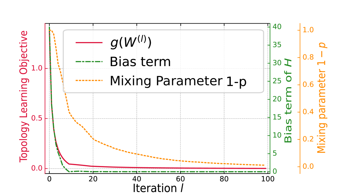
(a) Topology learning

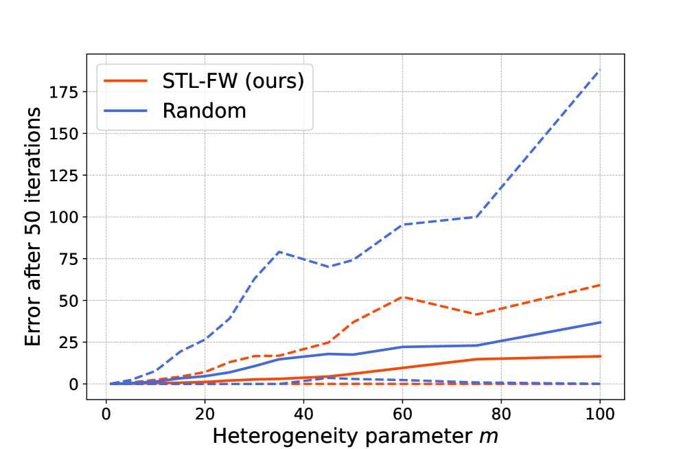
(b)  D-SGD with $d_{\text{max}}=3$

(c)  D-SGD with $d_{\text{max}}=9$

Figure 1: (a) Evolution of key quantities across the iterations of topology learning: in red the objective function $g(W^{(l)})$, in green the bias term $\sup_{\theta}\frac{1}{n}\sum_{i=1}^{n}\|\sum_{j=1}^{n}W^{(l)}_{ij}\nabla f_{j}(\theta)-\nabla f(\theta)\|_{2}^{2}$ and in yellow the mixing parameter $1-p=\lambda_{2}(W^{(l){\mkern-1.5mu\mathsf{T}}}W^{(l)})$. Here, $\lambda=0.5$ and $m=5$. (b, c) Error $n^{-1}\|\theta^{(t)}-\theta^{\star}\|_{2}^{2}$ (solid line) of D-SGD after $50$ iterations, averaged over $10$ runs, for increasing levels of heterogeneity (measured by parameter $m$). The dashed lines show $\max_{i}(\theta_{i}^{(t)}-\theta^{\star})^{2}$ and $\min_{i}(\theta_{i}^{(t)}-\theta^{\star})^{2}$, illustrating the variability across nodes.

The algorithm is summarized in Algorithm 2. Starting from the identity matrix $\widehat{W}^{(0)}=I_{n}\in\mathcal{S}$, each iteration $l\geq 0$ consists of moving towards a feasible point $P^{(l+1)}$ that minimizes a linearization of $g$ at the current iterate $\widehat{W}^{(l)}$. As finding $P^{(l+1)}$ is a linear problem, solving it over $\mathcal{S}$ is equivalent to solving it over $\mathcal{A}$. Although $\mathcal{A}$ contains $n!$ elements, the linear program corresponds to the well-known assignment problem (Burkard et al.,, 2012; Crouse,, 2016) and can be solved tractably with the Hungarian algorithm, which has a worst-case complexity of $\mathcal{O}(n^{3})$ (Lovász and Plummer,, 2009). Note that the gradient $\nabla g(W)$ needed to solve the assignment problem is given by

$$\textstyle\frac{2}{n}\sum_{k=1}^{K}(W\Pi_{:,k}-\overline{\Pi_{:,k}}\mathbf{1})\cdot\Pi_{:,k}^{\mkern-1.5mu\mathsf{T}}+\frac{2}{n}\lambda\left(W-\frac{\mathbf{1}\mathbf{1}^{\mkern-1.5mu\mathsf{T}}}{n}\right)~{},$$

where $\Pi_{:,k}$ is the $k$-th column of $\Pi$. The next iterate $\widehat{W}^{(l+1)}$ is then obtained as a convex combination of $P^{(l+1)}$ and $\widehat{W}^{(l)}$, and is thus guaranteed to be in $\mathcal{S}$. The optimal combining weight is computed by line-search, which has a closed-form solution since $g$ is quadratic (see Appendix C.2).

Crucially, Algorithm 2 allows to control the sparsity of the final solution: since a permutation matrix contains exactly one non-zero entry in each row and each column, at most one new incoming and one new outgoing edge per node are added. As we start from the identity matrix (i.e., only self-edges), this guarantees that at the end of the $l$-th iteration, each node will have at most $l$ in-neighbors and $l$ out-neighbors. The per-iteration communication complexity of D-SGD induced by the learned topology can thus be directly controlled by the number of iterations of our algorithm. The trade-off with the quality of the solution is quantified by the following theorem, which is derived from standard results for FW (Jaggi,, 2013) combined with a tight bound on the smoothness of $g$ in appropriate norm (see Appendix C).

Theorem 2.

Consider the statistical setup presented in Section 5.1 and let $\{\widehat{W}^{(l)}\}^{L}_{l=1}$ be the sequence of mixing matrices generated by Algorithm 2. Then, at any iteration $l=1,\ldots,L$, we have:

$$g(\widehat{W}^{(l)})\leq\frac{16}{l+2}\big{(}\lambda+\frac{1}{n}\big{\|}\sum_{k=1}^{K}(\Pi_{:,k}-\overline{\Pi_{:,k}}\mathbf{1})\cdot\Pi_{:,k}^{\mkern-1.5mu\mathsf{T}}\big{\|}^{\star}_{2}\big{)}~{},$$ (9)

where $\left\|\cdot\right\|^{\star}_{2}$ stands for the nuclear norm, i.e., the sum of singular values. Furthermore, we have $d^{\text{in}}_{\text{max}}(\widehat{W}^{(l)})\leq l$ and $d^{\text{out}}_{\text{max}}(\widehat{W}^{(l)})\leq l$, resulting in a per-iteration complexity bounded by $l$.

The above theorem shows that the objective $g$ decreases at a rate of $\mathcal{O}(1/l)$ as new connections between nodes are made. In general, we can bound (9) less tightly by $g(\widehat{W}^{(l)})\leq\frac{16}{l+2}\left(\lambda+1\right)$, which is independent of the number of nodes $n$. Recall that with $\lambda=\sigma_{\max}^{2}/KB$, the value $\bar{\tau}^{2}$ of Proposition 2 is exactly equal to $KB\cdot g(W)$. Therefore, the bound given in Theorem 2 directly bounds neighborhood heterogeneity and can thus be plugged in the rates of Theorem 1.

To summarize, our approach provides a principled way to learn the topology so as to reduce neighborhood heterogeneity while controlling the per-iteration communication complexity of D-SGD. Remarkably, the fact that $g(\widehat{W}^{(l)})$ is independent of $n$ implies that we can find topologies that approximately optimize the convergence rate of D-SGD while keeping the communication load per node constant, thereby guaranteeing scalability to a large number of nodes even in highly heterogeneous scenarios.

6 Experiments

This section shows the practical usefulness of our topology learning method, referred to as Sparse Topology Learning with Frank-Wolfe (STL-FW). We call communication budget $d_{\text{max}}=\max\{d^{\text{in}}_{\text{max}},d^{\text{out}}_{\text{max}}\}$ the maximal number of neighbors a node can have in the used topologies, which controls the per-iteration communication complexity incurred by any node.

6.1 Simulations on Synthetic Data

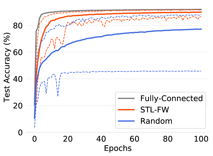
MNIST $d_{\max}=2$

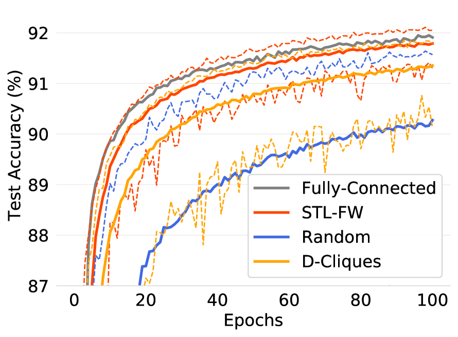
MNIST $d_{\max}=5$

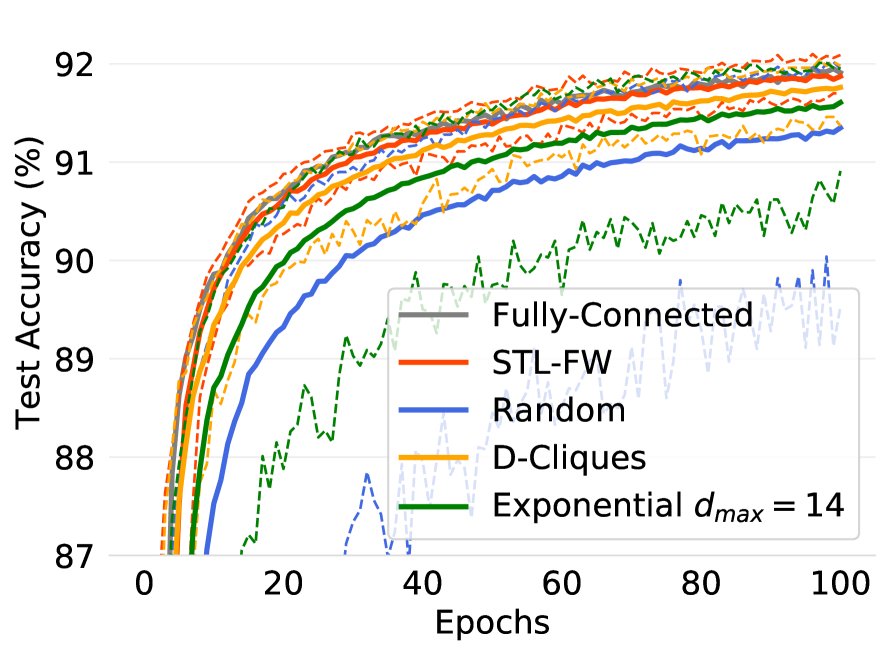
MNIST $d_{\max}=10$

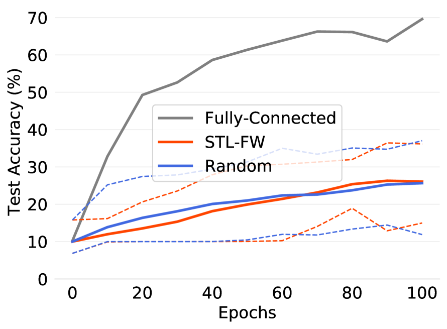
CIFAR10 $d_{\max}=2$

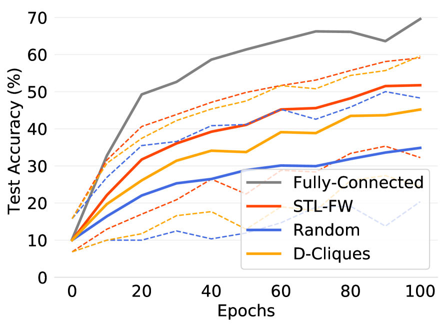
CIFAR10 $d_{\max}=5$

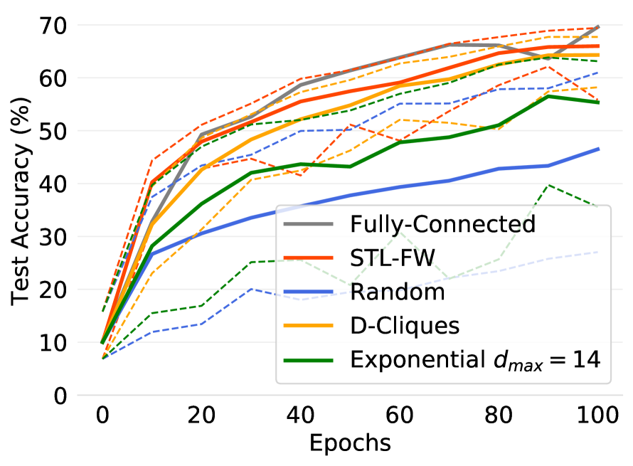
CIFAR10 $d_{\max}=10$

Figure 2: Convergence of D-SGD with STL-FW (our approach) and alternative topologies on real datasets under different communication budgets. The fully connected graph induces intractable communication costs but gives a performance upper bound, while the exponential graph is shown for $d_{\max}=10$ but exceeds this budget.

Statistical setup. We generalize the mean estimation objective of Example 1 with $K=10$ clusters and $n=100$ nodes, with exactly $10$ nodes associated to each cluster. Each cluster is associated with a specific Gaussian distribution, which corresponds to a class in the statistical framework described in Section 5.1. The variance of the $K$ distributions is the same ($\tilde{\sigma}^{2}=1$) but their means are evenly spread over $[-m,m]$. Thus, $m\geq 0$ controls the heterogeneity of the problem (the bigger $m$, the more heterogeneous the setup). We can analytically compute all numerical constants introduced throughout the paper. Unless otherwise noted, $\lambda$ is set to $\sigma^{2}/KB$ where $\sigma^{2}=4\tilde{\sigma}^{2}$ and $B=4m^{2}$.

Competitor. For a fixed budget $d_{\text{max}}$, we compare the topology learned by STL-FW to a random $d_{\text{max}}$-regular graph with uniform weights $\frac{1}{d_{\text{max}}+1}$. This graph is independent of the data but has good mixing parameter $p$ (every node will have exactly $b$ neighbors, with uniform weights). We use a fixed step-size for D-SGD, which is tuned separately for each topology in the interval $[0.001,1]$.

Results. We first study the behavior of our topology learning algorithm. As seen in Figure 1(a), the objective function $g(W^{(l)})$ decreases quickly in the first iterations with a clear elbow at $l=9$ iterations. This is because we have $K=10$ “classes”, hence $9$ neighbors are sufficient to compensate for label skew. We also see that decreasing $g$ successfully decreases the two key quantities that affect the convergence of D-SGD and are upper bounded by $g$: the bias term in Equation (4) (which does not depend on $\theta$ in this setup and can therefore be computed exactly) and the mixing parameter $1-p$ (which continues to decrease beyond $l=9$).

Figure 1(b, c) shows that the topology learned by STL-FW indeed translates into faster convergence for D-SGD than with the random (but well-connected) topology in data heterogeneous settings. This is especially striking when looking at best and worst-case errors across nodes (dashed lines). For a low budget ($d_{\text{max}}=3$), D-SGD with our topology remains slightly impacted by heterogeneity. But remarkably, for $d_{\text{max}}=9$, our topology makes D-SGD completely insensitive to increasing data heterogeneity. This observation is consistent with the elbow observed at $l=d_{\text{max}}=9$ in Figure 1(a). In Appendix D.2, we provide basic statistics on the topologies obtained for the two budgets $d_{\text{max}}=3$ and $d_{\text{max}}=9$. We can see in particular that the topologies obtained with STL-FW are $d_{\text{max}}$-regular (like the random graph) but have much lower bias (i.e., the distribution of labels in the neighborhood of nodes is closer to the global distribution). As expected, this bias is equal to $0$ for $d_{\text{max}}=9$.

6.2 Experiments on Real Datasets

Setup. We follow the experimental setup in Bellet et al., (2022) and consider two classification tasks: a linear model on MNIST (Deng,, 2012) and a Group Normalized LeNet (Hsieh et al.,, 2020) on CIFAR10 (Krizhevsky et al.,, 2009). In both cases, we partition the dataset on 100 nodes using the scheme introduced in McMahan et al., (2017), i.e. on average, nodes will have examples of two classes, but may have only 1 and up to 4. We re-use the hyper-parameters from Bellet et al., (2022): a learning rate of 0.1 and batch size of 128 for MNIST, and a learning rate of 0.002 and batch size of 20 for CIFAR10. Using D-SGD, we compare the topology learned with our approach STL-FW to other fixed topologies: (1) a fully-connected graph ($d_{\max}=99$), which exhibits the fastest convergence speed but is impractical, (2) a random graph with the same communication budget as STL-FW, (3) D-Cliques (Bellet et al.,, 2022), also with the same budget, and (4) a deterministic exponential graph promoted in recent work (Ying et al.,, 2021) ($d_{\max}=14$). Note that all competing topologies are data-independent, except D-Cliques. To have a fair comparison, we use standard D-SGD without algorithmic modifications like “clique-averaging” introduced by Bellet et al., (2022). For all experiments with STL-FW, we use $\lambda=0.1$ since, remarkably, its value does not significantly change the results (see Figure  3 in Appendix D).

Results. Figure 2 shows our results for varying communication budget $d_{max}$: small ($2$), medium ($5$) and large ($10$). On MNIST, STL-FW makes convergence faster than all competitors and quickly matches the speed of the fully-connected topology as the budget $d_{\max}$ increases. Remarkably, STL-FW is already showing good performance at $d_{\max}=2$, which is a very small budget that the other topologies (except the random one) cannot handle. As expected, the two data-dependent topologies (D-Cliques and STL-FW) outperform the random topologies, including the exponential graph which has better connectivity ($d_{\max}=14$) but does not compensate for the heterogeneity. The fact that STL-FW improves over D-Cliques can be explained by the fact that D-Cliques only compensate the heterogeneity (the bias term in Equation (4)) without consideration for the overall connectivity (the variance term in Equation (4)). This is illustrated in the tables of Appendix D.2.

On CIFAR10, we see that $d_{\max}=2$ is not sufficient to reach good performance. This can be explained by the increased complexity of the problem (non-convex objective with a deep model), requiring larger communication budgets. This is in line with empirical results in prior work (Kong et al.,, 2021). However, with slightly larger budgets i.e. $d_{\max}=5$ and $10$ ($d_{\max}=3$ in Fig. 5, App. D), performance improves and the results are consistent with those on MNIST: STL-FW outperforms other sparse topologies and comes close to the performance of the fully connected topology for $d_{\max}=10$. Overall, STL-FW provides better convergence speed than all tractable alternatives, with the additional ability to operate in low communication regimes (unlike D-Cliques and the exponential graph).

7 Conclusion

This paper addressed two important open problems in decentralized learning. First, thanks to our new notion of neighborhood heterogeneity, we characterized the joint effect of the topology and the data heterogeneity in the convergence rate of D-SGD. Our results show that, if chosen appropriately, the topology can compensate for the heterogeneity and speed up convergence. Second, we tackled the problem of learning a good topology under data heterogeneity. To the best of our knowledge, our work is the first to provide a principled and data-dependent approach, with explicit control on the trade-off between the communication costs and the convergence speed of D-SGD. We believe that our work paves the way for the design of other data-dependent topology learning techniques. One may for instance investigate different types of heterogeneity (beyond label skew), different knowledge assumptions (e.g., not knowing the proportions), and dynamic learning of the topology. We can also envision fully decentralized and privacy-preserving versions.

Appendix

Appendix A Details on Example 1

In this section, we provide more details on Example 1 (Section 4.1) by giving the exact parametrization. Recall that we want to find an example where Assumption 5 is not verified while Assumption 4 is.

Let us consider $n$ nodes with $n$ an even number. For all $i=1,\ldots,n$, assume $Z_{i}\sim\mathcal{N}(m,\tilde{\sigma}^{2})$ if $i$ is odd and $Z_{i}\sim\mathcal{N}(-m,\tilde{\sigma}^{2})$ if $i$ is even. Assume further that $\tilde{\sigma}^{2}<+\infty$ but $m>0$ can be asymptotically large. For all $i=1,\ldots,n$ we fix $F_{i}(\theta,Z_{i})=(\theta-Z_{i})^{2}$, which corresponds to a simple mean estimation objective.

Consider a fixed mixing matrix $W$ associated with a ring topology that alternates between the two distributions. Specifically, for $i=2,\ldots,n-1$ and $j=1,\ldots,n$, we fix the weights as follows:

$$W_{ij}=\left\{\begin{array}[]{ll}\frac{1}{2}\hskip 10.00002pt\text{if}\hskip 5.0ptj=i~{},\\ \frac{1}{4}\hskip 10.00002pt\text{if}\hskip 5.0ptj=i+1\hskip 5.0pt\text{or}\hskip 5.0ptj=i-1~{},\\ 0\hskip 10.00002pt\text{otherwise}~{}.\end{array}\right.$$

Moreover, we fix $W_{11}=W_{nn}=\frac{1}{2}$ and $W_{1n}=W_{n1}=\frac{1}{4}$.

With such parametrization we have $\nabla F_{i}(\theta,Z_{i})=2(\theta-Z_{i})$ and therefore $\nabla f_{i}(\theta)=2(\theta-m)$ if $i$ is odd and $\nabla f_{i}(\theta)=2(\theta+m)$ if $i$ is even. Moreover, the gradient of the global objective is $\nabla f(\theta)=\frac{1}{n}\sum_{i}\nabla f_{i}(\theta)=2\theta$ and the neighborhood averaging $\sum_{j}W_{ij}\nabla f_{j}(\theta)=2\theta$ for all $i$.

We first verify that Assumptions 2 is satisfied:

$$\mathbb{E}\left[\left(\nabla F_{i}(\theta,Z_{i})-\nabla f_{i}(\theta)\right)^{2}\right]=\mathbb{E}\left[4\left(Z_{i}-\mathbb{E}Z_{i}\right)^{2}\right]=4\tilde{\sigma}^{2}<\infty~{}.$$

Let us now find a bound $\bar{\tau}^{2}$ on the neighborhood heterogeneity. Using a bias-variance decomposition, we have:

$$H(\theta) =\frac{1}{n}\sum_{i=1}^{n}\mathbb{E}\Bigg{(}\sum_{j=1}^{n}W_{ij}\nabla F_{j}(\theta)-\frac{1}{n}\sum_{j=1}^{n}\nabla F_{j}(\theta)\Bigg{)}^{2}$$

$$=\frac{1}{n}\sum_{i=1}^{n}\Big{(}\sum_{j=1}^{n}W_{ij}\nabla f_{j}(\theta)-\frac{1}{n}\sum_{j=1}^{n}\nabla f_{j}(\theta)\Big{)}^{2}+\frac{1}{n}\sum_{i=1}^{n}\mathbb{E}\Big{(}\sum_{j=1}^{n}(W_{ij}-\frac{1}{n})(\nabla f_{j}(\theta)-\nabla F_{j}(\theta))\Big{)}^{2}$$

$$=\frac{1}{n}\sum_{i=1}^{n}\left(2\theta-2\theta\right)^{2}+\frac{1}{n}\sum_{i=1}^{n}\sum_{j=1}^{n}(W_{ij}-\frac{1}{n})^{2}\mathbb{E}(\nabla f_{j}(\theta)-\nabla F_{j}(\theta))^{2}$$

$$=0+4\tilde{\sigma}^{2}\frac{1}{n}\sum_{i=1}^{n}\sum_{j=1}^{n}(W_{ij}-\frac{1}{n})^{2}\leq 4\tilde{\sigma}^{2}~{}.$$

The third equality was obtained thanks to the fact that $\mathbb{E}[\nabla f_{j}(\theta)-\nabla F_{j}(\theta)]=0$. This result shows that Assumption 4 is verified with $\bar{\tau}^{2}=4\tilde{\sigma}^{2}<\infty$.

On the contrary, since $m$ can be arbitrary large, Assumption 5 is not verified. Indeed:

$$\frac{1}{n}\sum_{i=1}^{n}\left(\nabla f_{i}(\theta)-\frac{1}{n}\sum_{j=1}^{n}\nabla f_{j}(\theta)\right)^{2} =\frac{1}{n}\sum_{i=1}^{n}(2m)^{2}$$

$$=\frac{4m^{2}}{n}\triangleq\bar{\zeta}^{2}\underset{m\rightarrow\infty}{\longrightarrow}+\infty~{}.$$

Remark. At first sight, one may wonder why the local variance term $\tilde{\sigma}^{2}$ appears in $\bar{\tau}^{2}$ but not in $\bar{\zeta}^{2}$. This is because we chose to define neighborhood heterogeneity in expectation with respect to the pointwise loss functions $F_{1},\dots,F_{n}$, resulting in a bias-variance decomposition (see Eq. 4) which is the relevant quantity to optimize when learning the topology in Section 5. In contrast, following the convention used in previous work, local heterogeneity is defined with respect to the local objectives $f_{1},\dots,f_{n}$ and thus only measures a bias term, while the variance term is accounted separately by Assumption 2. Since the variance terms are the same in both settings, the difference is in how the bias term is measured (at the node level or at the neighborhood level): in the example above, it is equal to $\frac{4m^{2}}{n}$ for local heterogeneity while it is equal to $0$ for neighborhood heterogeneity (see the above calculation of $H(\theta)$).

Appendix B Proof of Theorem 1

B.1 Notations and Overview

We start by re-writing the updates of D-SGD (Algorithm 1) in matrix form.

Let $\Theta^{(t)}\triangleq\left(\theta_{1}^{(t)},\ldots,\theta_{n}^{(t)}\right)\in\mathbb{R}^{d\times n}$ be the matrix that contains the parameter vectors of all nodes at time $t$. Denote by $\nabla F(\Theta^{(t)},Z^{(t)})\triangleq\left(\nabla F_{1}(\theta^{(t)}_{1},Z^{(t)}_{1}),\ldots,\nabla F_{n}(\theta^{(t)}_{n},Z^{(t)}_{n})\right)\in\mathbb{R}^{d\times n}$ the matrix containing all stochastic gradients at time $t$. The D-SGD update at time $t$ can then be written as:

$$\Theta^{(t+1)}=\left(\Theta^{(t)}-\eta_{t}\nabla F(\Theta^{(t)},Z^{(t)})\right)W^{(t){\mkern-1.5mu\mathsf{T}}}~{}.$$

In the following, we denote $\overline{\Theta}^{(t)}\triangleq\left(\bar{\theta}^{(t)},\ldots,\bar{\theta}^{(t)}\right)=\Theta^{(t)}\cdot\frac{1}{n}\mathbf{1}\mathbf{1}^{\mkern-1.5mu\mathsf{T}}$.

The proof follows the classical steps found in the literature (see e.g. Koloskova et al., (2020); Neglia et al., (2020)). The main difference resides in how the consensus term $\|\Theta^{(t)}-\overline{\Theta}^{(t)}\|_{F}^{2}$ is controlled across iterations (Lemma 3). The proof is organized as follows.

Convex case.

1. Lemma 1 provides a descent recursion that allows to control the decreasing of the term $\left\|\bar{\theta}^{(t)}-\theta^{\star}\right\|^{2}$. The proof closely follows the one of Koloskova et al., (2020); Neglia et al., (2020).

2. In Lemma 3, the consensus term $\|\Theta^{(t)}-\overline{\Theta}^{(t)}\|_{F}^{2}$, which appears in the result of Lemma 1, is upper-bounded. The resulting upper-bound exhibits our new quantity $\bar{\tau}^{2}$ (an upper bound on neighborhood heterogeneity).

3. Corollary 1 uses the previous lemma to bound $\frac{1}{T+1}\sum_{t=0}^{T}\|\Theta^{(t)}-\overline{\Theta}^{(t)}\|_{F}^{2}$.

4. Lemma 4 provides an upper-bound on the error term with the following form:

   $$\frac{1}{T+1}\sum_{t=0}^{T}\mathbb{E}(f(\bar{\theta}^{(t)})-f^{\star})\leq 2\left(\frac{br_{0}}{T+1}\right)^{\frac{1}{2}}+2e^{\frac{1}{3}}\left(\frac{r_{0}}{T+1}\right)^{\frac{2}{3}}+\frac{dr_{0}}{T+1},$$

   where $b=\frac{\bar{\sigma}^{2}}{n}$, $e=\frac{36L\bar{\tau}^{2}}{p^{2}}$, $d=\frac{8L}{p}$ and $r_{0}=\|\theta^{(0)}-\theta^{\star}\|_{2}^{2}$.

5. To get the final rate of Theorem 1, it suffices to find $T$ such that each term in the right-hand side of the previous equation in bounded by $\frac{\varepsilon}{3}$.

   • $2\left(\frac{br_{0}}{T+1}\right)^{\frac{1}{2}}\leq\frac{\varepsilon}{3}\Longleftrightarrow\frac{36br_{0}}{\varepsilon^{2}}\leq T+1\Longleftrightarrow\frac{36\bar{\sigma}^{2}r_{0}}{n\varepsilon^{2}}\leq T+1$,

   • $2e^{\frac{1}{3}}\left(\frac{r_{0}}{T+1}\right)^{\frac{2}{3}}\leq\frac{\varepsilon}{3}\Longleftrightarrow\frac{e^{\frac{1}{2}}6^{\frac{3}{2}}r_{0}}{\varepsilon^{\frac{3}{2}}}\leq T+1\Longleftrightarrow\frac{6^{\frac{5}{2}}\sqrt{L}\bar{\tau}r_{0}}{p\varepsilon^{\frac{3}{2}}}\leq T+1$,

   • $\frac{dr_{0}}{T+1}\leq\frac{\varepsilon}{3}\Longleftrightarrow\frac{3dr_{0}}{\varepsilon}\leq T+1\Longleftrightarrow\frac{24Lr_{0}}{p\varepsilon}\leq T+1$.

   In particular, it suffices to take

   $$T\geq\frac{36\bar{\sigma}^{2}r_{0}}{n\varepsilon^{2}}+\frac{89\sqrt{L}\bar{\tau}r_{0}}{p\varepsilon^{\frac{3}{2}}}+\frac{24Lr_{0}}{p\varepsilon}=\mathcal{O}\left(\frac{\bar{\sigma}^{2}}{n\varepsilon^{2}}+\frac{\sqrt{L}\bar{\tau}}{p\varepsilon^{\frac{3}{2}}}+\frac{L}{p\varepsilon}\right)r_{0}~{},$$

   in order to have all three terms bounded by $\frac{\varepsilon}{3}$, and obtain the final result.

Non-convex case. The proof is similar to the convex one: it only differs in the descent lemmas that are used.

1. Lemma 2 provides the descent lemma for the non-convex scenario.

2. The consensus term is bounded using the same results as in the convex case, i.e., with Lemma 3 and Corollary 1.

3. Lemma 5 provides an upper-bound on the error term with the following form:

   $$\frac{1}{T+1}\sum_{t=0}^{T}\mathbb{E}\Big{\|}\nabla f(\bar{\theta}^{(t)})\Big{\|}_{2}^{2}\leq 2\left(\frac{4bf_{0}}{T+1}\right)^{\frac{1}{2}}+2e^{\frac{1}{3}}\left(\frac{4f_{0}}{T+1}\right)^{\frac{2}{3}}+\frac{4df_{0}}{T+1},$$

   where $b=\frac{2L\bar{\sigma}^{2}}{n}$, $e=\frac{96L^{2}\bar{\tau}^{2}}{p^{2}}$, $d=\frac{8L}{p}$ and $f_{0}=f(\theta^{(0)})-f^{\star}$.

4. We bound in each term of the previous equation by $\frac{\varepsilon}{3}$ and get the sufficient condition:

   $$T\geq\frac{288L\bar{\sigma}^{2}f_{0}}{n\varepsilon^{2}}+\frac{576L\bar{\tau}f_{0}}{p\varepsilon^{\frac{3}{2}}}+\frac{96Lf_{0}}{p\varepsilon}=\mathcal{O}\left(\frac{L\bar{\sigma}^{2}}{n\varepsilon^{2}}+\frac{L\bar{\tau}}{p\varepsilon^{\frac{3}{2}}}+\frac{L}{p\varepsilon}\right)f_{0}~{}.$$

B.2 Preliminaries and Useful Results

Property 1 (Averaging preservation).

Let $W\in\mathbb{R}^{n\times n}$ be a mixing matrix and $\Theta$ be any matrix in $\mathbb{R}^{d\times n}$. Then, $W$ preserves averaging:

$$(\Theta W)\frac{\mathbf{1}\mathbf{1}^{\mkern-1.5mu\mathsf{T}}}{n}=\Theta\frac{\mathbf{1}\mathbf{1}^{\mkern-1.5mu\mathsf{T}}}{n}=\overline{\Theta}$$ (10)

Property 2 (Implications of $L$-smoothness and convexity).

• If we assume convexity, we have for all $i\in\llbracket 1,\ldots,n\rrbracket$:

  $$\langle\nabla f_{i}(\tilde{\theta}),\tilde{\theta}-\theta\rangle\geq f_{i}(\tilde{\theta})-f_{i}(\theta).$$ (11)

• Under Assumption 1 ($L$-smoothness), it holds for all $i\in\llbracket 1,\ldots,n\rrbracket$:

  $$F_{i}(\theta,Z)\leq F_{i}(\tilde{\theta},Z)+\langle\nabla F_{i}(\tilde{\theta},Z),\theta-\tilde{\theta}\rangle+\frac{L}{2}\|\theta-\tilde{\theta}\|_{2}^{2},\quad\quad\quad\forall\theta,\tilde{\theta}\in\mathbb{R}^{d},Z\in\theta_{i}.$$ (12)

  Taking the expectation of the previous equation, we also have:

  $$f_{i}(\theta)\leq f_{i}(\tilde{\theta})+\langle\nabla F(\tilde{\theta}),\theta-\tilde{\theta}\rangle+\frac{L}{2}\|\theta-\tilde{\theta}\|_{2}^{2},\quad\quad\quad\quad\forall\theta,\tilde{\theta}\in\mathbb{R}^{d}.$$ (13)

• If we further assume that the $F_{i}$’s are convex, Assumption 1 also implies $\forall\theta,\tilde{\theta}\in\mathbb{R}^{d}$,$Z\in\theta_{i}$:

  $$\|\nabla f_{i}(\theta)-\nabla f_{i}(\tilde{\theta})\|_{2} \leq L\|\theta-\tilde{\theta}\|_{2},$$ (14)

  $$\|\nabla f_{i}(\theta)-\nabla f_{i}(\tilde{\theta})\|^{2}_{2} \leq 2L\left(f_{i}(\theta)-f_{i}(\tilde{\theta})-\big{\langle}\nabla f_{i}(\tilde{\theta}),\theta-\tilde{\theta}\big{\rangle}\right),$$ (15)

  $$\|\nabla F_{i}(\theta,Z)-\nabla F_{i}(\tilde{\theta},Z)\|^{2}_{2} \leq 2L\left(F_{i}(\theta,Z)-F_{i}(\tilde{\theta},Z)-\big{\langle}\nabla F_{i}(\tilde{\theta},Z),\theta-\tilde{\theta}\big{\rangle}\right).$$ (16)

These results can be found in many convex optimization books and papers, e.g. in Bubeck, (2014).

Property 3 (Norm inequalities).

• For a set of vectors $\{a_{i}\}_{i=1}^{n}$ such that $a_{i}\in\mathbb{R}^{d}$,

  $$\Big{\|}\sum_{i=1}^{n}a_{i}\Big{\|}_{2}^{2}\leq n\sum_{i=1}^{n}\left\|a_{i}\right\|_{2}^{2}.$$ (17)

• For two vectors $a,b\in\mathbb{R}^{d}$,

  $$\|a+b\|_{2}^{2}\leq(1+\alpha)\|a\|_{2}^{2}+(1+\alpha^{-1})\|b\|_{2}^{2},\quad\quad\quad\forall\alpha>0.$$ (18)

• For two vectors $a,b\in\mathbb{R}^{d}$,

  $$2\langle a,b\rangle\leq\alpha\|a\|_{2}^{2}+\alpha^{-1}\|b\|_{2}^{2},\quad\quad\quad\forall\alpha>0.$$ (19)

B.3 Needed Lemmas

In the following we denote by $\mathcal{F}_{t}=\sigma(Z^{(k)}|k\leq t)$ the natural filtration with respect to $Z^{(t)}=(Z_{1}^{(t)},\ldots,Z_{n}^{(t)})$. Remark that $\forall i=1,\ldots,n$ the iterates $\theta_{i}^{(t+1)}$ and $\bar{\theta}^{(t+1)}$ are in particular $\mathcal{F}_{t}$-measurable.

Lemma 1 (Descent Lemma - Convex case).

Consider the setting of Theorem 1 and let $\eta_{t}\leq\frac{1}{4L}$, then we almost surely have:

$$\mathbb{E}_{Z^{(t)}|\mathcal{F}_{t-1}}\left\|\bar{\theta}^{(t+1)}-\theta^{\star}\right\|^{2}\leq\left\|\bar{\theta}^{(t)}-\theta^{\star}\right\|^{2}+\frac{\eta_{t}^{2}\bar{\sigma}^{2}}{n}-\eta_{t}\left(f(\bar{\theta}^{(t)})-f^{\star}\right)+\frac{3L}{2n}\eta_{t}\left\|\Theta^{(t)}-\overline{\Theta}^{(t)}\right\|_{F}^{2},$$ (20)

where $\mathbb{E}_{Z^{(t)}|\mathcal{F}_{t-1}}$ stands for the conditional expectation $\mathbb{E}_{Z^{(t)}}[\cdot|\mathcal{F}_{t-1}]$.

Proof.

The proof closely follows the one in Koloskova et al., (2020). Using the recursion of D-SGD and since all mixing matrices are doubly stochastic and preserve the average (Proposition 1) we have:

$$\|\bar{\theta}^{(t+1)} -\theta^{\star}\|^{2}=\left\|\bar{\theta}^{(t)}-\frac{\eta_{t}}{n}\sum_{i=1}^{n}\nabla F_{i}(\theta_{i}^{(t)},Z_{i}^{(t)})-\theta^{\star}\right\|^{2}$$

$$=\left\|\bar{\theta}^{(t)}-\theta^{\star}-\frac{\eta_{t}}{n}\sum_{i=1}^{n}\nabla f_{i}(\theta_{i}^{(t)})+\frac{\eta_{t}}{n}\sum_{i=1}^{n}\nabla f_{i}(\theta_{i}^{(t)})-\frac{\eta_{t}}{n}\sum_{i=1}^{n}\nabla F_{i}(\theta_{i}^{(t)},Z_{i}^{(t)})\right\|^{2}$$

$$=\left\|\bar{\theta}^{(t)}-\theta^{\star}-\frac{\eta_{t}}{n}\sum_{i=1}^{n}\nabla f_{i}(\theta_{i}^{(t)})\right\|^{2}+\eta_{t}^{2}\left\|\frac{1}{n}\sum_{i=1}^{n}\nabla f_{i}(\theta_{i}^{(t)})-\frac{1}{n}\sum_{i=1}^{n}\nabla F_{i}(\theta_{i}^{(t)},Z_{i}^{(t)})\right\|^{2}$$

$$\quad\quad\quad+2\left\langle\bar{\theta}^{(t)}-\theta^{\star}-\frac{\eta_{t}}{n}\sum_{i=1}^{n}\nabla f_{i}(\theta_{i}^{(t)}),\frac{\eta_{t}}{n}\sum_{i=1}^{n}\nabla f_{i}(\theta_{i}^{(t)})-\frac{\eta_{t}}{n}\sum_{i=1}^{n}\nabla F_{i}(\theta_{i}^{(t)},Z_{i}^{(t)})\right\rangle.$$

Passing to the conditional expectation, the last term (the inner product) is equal to $0$. This comes from the fact that $\mathbb{E}_{Z_{i}^{(t)}|\mathcal{F}_{t-1}}[\nabla F_{i}(\theta_{i}^{(t)},Z_{i}^{(t)})]=\nabla f_{i}(\theta_{i}^{(t)})$. We therefore need to bound the first two terms in the conditional expectation.

The second one can easily be bounded using Assumption 2:

$$\eta_{t}^{2}\mathbb{E}_{Z^{(t)}|\mathcal{F}_{t-1}}\Big{\|}\frac{1}{n}\sum_{i=1}^{n}\nabla f_{i}(\theta_{i}^{(t)})-\frac{1}{n}\sum_{i=1}^{n} \nabla F_{i}(\theta_{i}^{(t)},Z_{i}^{(t)})\Big{\|}^{2}$$

$$=\frac{\eta_{t}^{2}}{n^{2}}\mathbb{E}_{Z^{(t)}|\mathcal{F}_{t-1}}\Big{\|}\sum_{i=1}^{n}(\nabla f_{i}(\theta_{i}^{(t)})-\nabla F_{i}(\theta_{i}^{(t)},Z_{i}^{(t)}))\Big{\|}^{2}$$

$$=\frac{\eta_{t}^{2}}{n^{2}}\sum_{i=1}^{n}\mathbb{E}_{Z_{i}^{(t)}|\mathcal{F}_{t-1}}\Big{\|}\nabla f_{i}(\theta_{i}^{(t)})-\nabla F_{i}(\theta_{i}^{(t)},Z_{i}^{(t)})\Big{\|}^{2}$$

$$\overset{(A.\ref{ass:variance})}{\leq}\frac{\eta_{t}^{2}\bar{\sigma}^{2}}{n},$$

where the second equality was obtained using the identity $\mathbb{E}\left\|\sum_{i}Y_{i}\right\|_{2}^{2}=\sum_{i}\mathbb{E}\|Y_{i}\|_{2}^{2}$ when $Y_{i}$ are independent and $\mathbb{E}Y_{i}=0$.

Now that the second term is bounded, we can move to the first one. Because $\theta_{i}^{(t)}$ and $\bar{\theta}^{(t)}$ are $\mathcal{F}_{t-1}$-measurable, we have

$$\mathbb{E}_{Z^{(t)}|\mathcal{F}_{t-1}} \left\|\bar{\theta}^{(t)}-\theta^{\star}-\frac{\eta_{t}}{n}\sum_{i=1}^{n}\nabla f_{i}(\theta_{i}^{(t)})\right\|^{2}=\left\|\bar{\theta}^{(t)}-\theta^{\star}-\frac{\eta_{t}}{n}\sum_{i=1}^{n}\nabla f_{i}(\theta_{i}^{(t)})\right\|^{2}$$

$$=\left\|\bar{\theta}^{(t)}-\theta^{\star}\right\|^{2}+\eta_{t}^{2}\underbrace{\left\|\frac{1}{n}\sum_{i=1}^{n}\nabla f_{i}(\theta_{i}^{(t)})\right\|^{2}}_{T_{1}}-\underbrace{2\eta_{t}\left\langle\bar{\theta}^{(t)}-\theta^{\star},\frac{1}{n}\sum_{i=1}^{n}\nabla f_{i}(\theta_{i}^{(t)})\right\rangle}_{T_{2}}.$$

In order to bound $T_{1}$, recall that by definition $\frac{1}{n}\sum_{i}\nabla f_{i}(\theta^{\star})=0$, therefore:

$$T_{1} =\left\|\frac{1}{n}\sum_{i=1}^{n}(\nabla f_{i}(\theta_{i}^{(t)})-\nabla f_{i}(\bar{\theta}^{(t)})+\nabla f_{i}(\bar{\theta}^{(t)})-\nabla f_{i}(\theta^{\star}))\right\|^{2}$$

$$\overset{(\ref{eq:norm_sum})}{\leq}2\left\|\frac{1}{n}\sum_{i=1}^{n}(\nabla f_{i}(\theta_{i}^{(t)})-\nabla f_{i}(\bar{\theta}^{(t)}))\right\|^{2}+2\left\|\frac{1}{n}\sum_{i=1}^{n}(\nabla f_{i}(\bar{\theta}^{(t)})-\nabla f_{i}(\theta^{\star}))\right\|^{2}$$

$$\overset{(\ref{eq:norm_sum})}{\leq}\frac{2}{n}\sum_{i=1}^{n}\left\|\nabla f_{i}(\theta_{i}^{(t)})-\nabla f_{i}(\bar{\theta}^{(t)})\right\|^{2}+\frac{2}{n}\sum_{i=1}^{n}\left\|\nabla f_{i}(\bar{\theta}^{(t)})-\nabla f_{i}(\theta^{\star})\right\|^{2}$$

$$\overset{(\ref{eq:f_i_smooth})(\ref{eq:f_i_smooth2})}{\leq}\frac{2L^{2}}{n}\sum_{i=1}^{n}\left\|\theta_{i}^{(t)}-\bar{\theta}^{(t)}\right\|^{2}+\frac{4L}{n}\sum_{i=1}^{n}\left(f_{i}(\bar{\theta}^{(t)})-f_{i}(\theta^{\star})-\left\langle\nabla f_{i}(\theta^{\star}),\bar{\theta}^{(t)}-\theta^{\star}\right\rangle\right)$$

$$=\frac{2L^{2}}{n}\sum_{i=1}^{n}\left\|\theta_{i}^{(t)}-\bar{\theta}^{(t)}\right\|^{2}+\frac{4L}{n}\sum_{i=1}^{n}\left(f_{i}(\bar{\theta}^{(t)})-f_{i}(\theta^{\star})\right)-4L\left\langle\underbrace{\frac{1}{n}\sum_{i=1}^{n}\nabla f_{i}(\theta^{\star})}_{=0},\bar{\theta}^{(t)}-\theta^{\star}\right\rangle$$

$$=\frac{2L^{2}}{n}\sum_{i=1}^{n}\left\|\theta_{i}^{(t)}-\bar{\theta}^{(t)}\right\|^{2}+4L\left(f(\bar{\theta}^{(t)})-f^{\star}\right).$$

Finally, we have to bound $T_{2}$:

$$-T_{2} =-\frac{2\eta_{t}}{n}\sum_{i=1}^{n}\left\langle\bar{\theta}^{(t)}-\theta^{\star},\nabla f_{i}(\theta_{i}^{(t)})\right\rangle$$

$$=-\frac{2\eta_{t}}{n}\sum_{i=1}^{n}\left[\left\langle\bar{\theta}^{(t)}-\theta_{i}^{(t)},\nabla f_{i}(\theta_{i}^{(t)})\right\rangle+\left\langle\theta_{i}^{(t)}-\theta^{\star},\nabla f_{i}(\theta_{i}^{(t)})\right\rangle\right]$$

$$\overset{(\ref{eq:Lip_f_i})(\ref{eq:grad_conv})}{\leq}-\frac{2\eta_{t}}{n}\sum_{i=1}^{n}\left[f_{i}(\bar{\theta}^{(t)})-f_{i}(\theta_{i}^{(t)})-\frac{L}{2}\|\bar{\theta}^{(t)}-\theta_{i}^{(t)}\|_{2}^{2}+f_{i}(\theta_{i}^{(t)})-f_{i}(\theta^{\star})\right]$$

$$=-2\eta_{t}\left(f(\bar{\theta}^{(t)})-f(\theta^{\star})\right)+\frac{L\eta_{t}}{n}\sum_{i=1}^{n}\|\bar{\theta}^{(t)}-\theta_{i}^{(t)}\|_{2}^{2}$$

$$=-2\eta_{t}\left(f(\bar{\theta}^{(t)})-f^{\star}\right)+\frac{L\eta_{t}}{n}\|\overline{\Theta}^{(t)}-\Theta^{(t)}\|_{F}^{2}.$$

Combining all previous results, we get:

$$\mathbb{E}_{Z^{(t)}|\mathcal{F}_{t-1}}\left\|\bar{\theta}^{(t+1)}-\theta^{\star}\right\|^{2} \leq\left\|\bar{\theta}^{(t)}-\theta^{\star}\right\|^{2}+\frac{\eta_{t}^{2}\bar{\sigma}^{2}}{n}+\frac{L\eta_{t}}{n}\left(2L\eta_{t}+1\right)\|\overline{\Theta}^{(t)}-\Theta^{(t)}\|_{F}^{2}$$

$$\hskip 113.81102pt+2\eta_{t}\left(2L\eta_{t}-1\right)\left(f(\bar{\theta}^{(t)})-f^{\star}\right).$$

Since, by hypothesis, $\eta_{t}\leq\frac{1}{4L}$, we have $2L\eta_{t}+1\leq\frac{3}{2}$ and $2L\eta_{t}-1\leq-\frac{1}{2}$, which concludes the proof. ∎

Lemma 2 (Descent Lemma - Non-convex case).

Consider the setting of Theorem 1 and let $\eta_{t}\leq\frac{1}{4L}$, then we almost surely have:

$$\mathbb{E}_{Z^{(t)}|\mathcal{F}_{t-1}}f(\bar{\theta}^{(t+1)})-f^{\star}\leq f(\bar{\theta}^{(t)})-f^{\star}-\frac{\eta_{t}}{4}\|\nabla f(\bar{\theta}^{(t)})\|_{2}^{2}+\frac{L^{2}}{n}\eta_{t}\left\|\Theta^{(t)}-\overline{\Theta}^{(t)}\right\|_{F}^{2}+\frac{L\bar{\sigma}^{2}}{2n}\eta_{t}^{2}.$$ (21)

Proof.

The proof adapts the one of Lemma $10$ in Koloskova et al., (2020) to our setting.

$$\mathbb{E}_{Z^{(t)}|\mathcal{F}_{t-1}}f(\bar{\theta}^{(t+1)})=\mathbb{E}_{Z^{(t)}|\mathcal{F}_{t-1}}f\Big{(}\bar{\theta}^{(t)}-\frac{\eta_{t}}{n}\sum_{i=1}^{n}\nabla F_{i}(\theta_{i}^{(t)},Z_{i}^{(t)})\Big{)}$$

$$\quad\overset{\eqref{eq:Lip_f_i}}{\leq}f(\bar{\theta}^{(t)})-\mathbb{E}_{Z^{(t)}|\mathcal{F}_{t-1}}\Big{\langle}\nabla f(\bar{\theta}^{(t)}),\frac{\eta_{t}}{n}\sum_{i=1}^{n}\nabla F_{i}(\theta_{i}^{(t)},Z_{i}^{(t)})\Big{\rangle}$$

$$+\frac{L}{2}\mathbb{E}_{Z^{(t)}|\mathcal{F}_{t-1}}\Big{\|}\frac{\eta_{t}}{n}\sum_{i=1}^{n}\nabla F_{i}(\theta_{i}^{(t)},Z_{i}^{(t)})\Big{\|}_{2}^{2}$$

$$\quad=f(\bar{\theta}^{(t)})\underbrace{-\Big{\langle}\nabla f(\bar{\theta}^{(t)}),\frac{\eta_{t}}{n}\sum_{i=1}^{n}\nabla f_{i}(\theta_{i}^{(t)})\Big{\rangle}}_{\triangleq T_{4}}+\frac{L\eta_{t}^{2}}{2}\underbrace{\mathbb{E}_{Z^{(t)}|\mathcal{F}_{t-1}}\Big{\|}\frac{1}{n}\sum_{i=1}^{n}\nabla F_{i}(\theta_{i}^{(t)},Z_{i}^{(t)})\Big{\|}_{2}^{2}}_{\triangleq T_{5}}$$

Adding and subtracting $\eta_{t}\nabla f(\bar{\theta}^{(t)})$ in $T_{4}$, we have

$$T_{4} =-\eta_{t}\Big{\|}\nabla f(\bar{\theta}^{(t)})\Big{\|}_{2}^{2}+\frac{\eta_{t}}{n}\sum_{i=1}^{n}\Big{\langle}\nabla f(\bar{\theta}^{(t)}),\nabla f_{i}(\bar{\theta}^{(t)})-\nabla f_{i}(\theta_{i}^{(t)})\Big{\rangle}$$

$$\overset{\eqref{eq:inner_alpha},\alpha=1}{\leq}-\eta_{t}\Big{\|}\nabla f(\bar{\theta}^{(t)})\Big{\|}_{2}^{2}+\frac{\eta_{t}}{2}\Big{\|}\nabla f(\bar{\theta}^{(t)})\Big{\|}_{2}^{2}+\frac{\eta_{t}}{2n}\sum_{i=1}^{n}\Big{\|}\nabla f_{i}(\bar{\theta}^{(t)})-\nabla f_{i}(\theta_{i}^{(t)})\Big{\|}_{2}^{2}$$

$$\overset{\eqref{eq:f_i_smooth}}{\leq}-\frac{\eta_{t}}{2}\Big{\|}\nabla f(\bar{\theta}^{(t)})\Big{\|}_{2}^{2}+\frac{L^{2}\eta_{t}}{2n}\sum_{i=1}^{n}\Big{\|}\bar{\theta}^{(t)}-\theta_{i}^{(t)}\Big{\|}_{2}^{2}~{}.$$

Let us now bound the term $T_{5}$:

$$T_{5} =\mathbb{E}_{Z^{(t)}|\mathcal{F}_{t-1}}\Big{\|}\frac{1}{n}\sum_{i=1}^{n}\nabla F_{i}(\theta_{i}^{(t)},Z_{i}^{(t)})-\frac{1}{n}\sum_{i=1}^{n}\nabla f_{i}(\theta_{i}^{(t)})+\frac{1}{n}\sum_{i=1}^{n}\nabla f_{i}(\theta_{i}^{(t)})\Big{\|}_{2}^{2}$$

$$=\frac{1}{n^{2}}\mathbb{E}_{Z^{(t)}|\mathcal{F}_{t-1}}\Big{\|}\sum_{i=1}^{n}\nabla F_{i}(\theta_{i}^{(t)},Z_{i}^{(t)})-\sum_{i=1}^{n}\nabla f_{i}(\theta_{i}^{(t)})\Big{\|}_{2}^{2}+\Big{\|}\frac{1}{n}\sum_{i=1}^{n}\nabla f_{i}(\theta_{i}^{(t)})\Big{\|}_{2}^{2}$$

$$\overset{(A.\ref{ass:variance})}{=}\frac{\bar{\sigma}^{2}}{n}+\Big{\|}\frac{1}{n}\sum_{i=1}^{n}\nabla f_{i}(\theta_{i}^{(t)})-\nabla f(\bar{\theta}^{(t)})+\nabla f(\bar{\theta}^{(t)})\Big{\|}_{2}^{2}$$

$$\overset{\eqref{eq:norm_sum}}{\leq}\frac{\bar{\sigma}^{2}}{n}+2\Big{\|}\frac{1}{n}\sum_{i=1}^{n}\nabla f_{i}(\theta_{i}^{(t)})-\nabla f(\bar{\theta}^{(t)})\Big{\|}_{2}^{2}+2\Big{\|}\nabla f(\bar{\theta}^{(t)})\Big{\|}_{2}^{2}$$

$$\overset{\eqref{eq:norm_sum}}{\leq}\frac{\bar{\sigma}^{2}}{n}+\frac{2}{n}\sum_{i=1}^{n}\Big{\|}\nabla f_{i}(\theta_{i}^{(t)})-\nabla f_{i}(\bar{\theta}^{(t)})\Big{\|}_{2}^{2}+2\Big{\|}\nabla f(\bar{\theta}^{(t)})\Big{\|}_{2}^{2}$$

$$\overset{\eqref{eq:f_i_smooth}}{\leq}\frac{\bar{\sigma}^{2}}{n}+\frac{2L^{2}}{n}\sum_{i=1}^{n}\Big{\|}\theta_{i}^{(t)}-\bar{\theta}^{(t)}\Big{\|}_{2}^{2}+2\Big{\|}\nabla f(\bar{\theta}^{(t)})\Big{\|}_{2}^{2}.$$

Next, plugging $T_{4}$ and $T_{5}$ into the first inequality, we have:

$$\mathbb{E}_{Z^{(t)}|\mathcal{F}_{t-1}}f(\bar{\theta}^{(t+1)})$$

$$\quad\leq f(\bar{\theta}^{(t)})-\eta_{t}\Big{(}\frac{1}{2}-L\eta_{t}\Big{)}\Big{\|}\nabla f(\bar{\theta}^{(t)})\Big{\|}_{2}^{2}+\Big{(}\frac{L^{2}\eta_{t}}{2n}+\frac{L^{3}\eta_{t}^{2}}{n}\Big{)}\left\|\Theta^{(t)}-\overline{\Theta}^{(t)}\right\|_{F}^{2}+\frac{L\bar{\sigma}^{2}}{2n}\eta_{t}^{2}~{}.$$

Since by hypothesis $\eta_{t}\leq\frac{1}{4L}$, we have $\frac{1}{2}-L\eta_{t}\geq\frac{1}{4}$ and $\frac{L^{2}\eta_{t}}{2n}+\frac{L^{3}\eta_{t}^{2}}{n}\leq\frac{L^{2}\eta_{t}}{n}$, we therefore get

$$\mathbb{E}_{Z^{(t)}|\mathcal{F}_{t-1}}f(\bar{\theta}^{(t+1)})\leq f(\bar{\theta}^{(t)})-\frac{\eta_{t}}{4}\Big{\|}\nabla f(\bar{\theta}^{(t)})\Big{\|}_{2}^{2}+\frac{L^{2}\eta_{t}}{n}\left\|\Theta^{(t)}-\overline{\Theta}^{(t)}\right\|_{F}^{2}+\frac{L\bar{\sigma}^{2}}{2n}\eta_{t}^{2}~{}.$$

Subtracting each side of the equation by $f^{\star}$, we obtain the final result. ∎

Lemma 3 (Consensus Control).

Consider the setting of Theorem 1 and let $\eta_{t}\leq\frac{p}{8L}$, then:

$$\mathbb{E}\left\|\Theta^{(t)}-\overline{\Theta}^{(t)}\right\|_{F}^{2}\leq(1-\frac{p}{4})\mathbb{E}\left\|\Theta^{(t-1)}-\overline{\Theta}^{(t-1)}\right\|_{F}^{2}+\frac{6n\bar{\tau}^{2}}{p}\eta_{t-1}^{2}.$$ (22)

Proof.

For any $\alpha>0$, we have:

$$\mathbb{E} \left\|\Theta^{(t)}-\overline{\Theta}^{(t)}\right\|_{F}^{2}=\mathbb{E}\left\|\Theta^{(t)}\left(I-\frac{\mathbf{1}\mathbf{1}^{\mkern-1.5mu\mathsf{T}}}{n}\right)\right\|_{F}^{2}$$

$$=\mathbb{E}\left\|\left(\Theta^{(t-1)}-\eta_{t-1}\nabla F(\Theta^{(t-1)},Z^{(t-1)})\right)W^{(t-1){\mkern-1.5mu\mathsf{T}}}\left(I-\frac{\mathbf{1}\mathbf{1}^{\mkern-1.5mu\mathsf{T}}}{n}\right)\right\|_{F}^{2}$$

$$\overset{(\ref{eq:preserve_ave})}{=}\mathbb{E}\left\|\left(\Theta^{(t-1)}-\eta_{t-1}\nabla F(\Theta^{(t-1)},Z^{(t-1)})\right)\left(W^{(t-1){\mkern-1.5mu\mathsf{T}}}-\frac{\mathbf{1}\mathbf{1}^{\mkern-1.5mu\mathsf{T}}}{n}\right)\right\|_{F}^{2}$$

$$\overset{(\ref{eq:norm_alpha})}{\leq}(1+\alpha)\mathbb{E}\left\|\Theta^{(t-1)}\left(W^{(t-1){\mkern-1.5mu\mathsf{T}}}-\frac{\mathbf{1}\mathbf{1}^{\mkern-1.5mu\mathsf{T}}}{n}\right)\right\|_{F}^{2}$$

$$+(1+\alpha^{-1})\eta_{t-1}^{2}\underbrace{\mathbb{E}\left\|\nabla F(\Theta^{(t-1)},Z^{(t-1)})\left(W^{(t-1){\mkern-1.5mu\mathsf{T}}}-\frac{\mathbf{1}\mathbf{1}^{\mkern-1.5mu\mathsf{T}}}{n}\right)\right\|_{F}^{2}}_{T_{3}}$$

$$\overset{(A.\ref{ass:rho})}{\leq}(1+\alpha)(1-p)\mathbb{E}\left\|\Theta^{(t-1)}-\overline{\Theta}^{(t-1)}\right\|_{F}^{2}+(1+\alpha^{-1})\eta_{t-1}^{2}T_{3}.$$

We now bound $T_{3}$ by relying on Assumption 4:

$$T_{3} =\mathbb{E}\Bigg{\|}\left(\nabla F(\Theta^{(t-1)},Z^{(t-1)})-\nabla F(\overline{\Theta}^{(t-1)},Z^{(t-1)})+\nabla F(\overline{\Theta}^{(t-1)},Z^{(t-1)})\right)\cdot$$

$$\hskip 284.52756pt\cdot\left(W^{(t-1){\mkern-1.5mu\mathsf{T}}}-\frac{\mathbf{1}\mathbf{1}^{\mkern-1.5mu\mathsf{T}}}{n}\right)\Bigg{\|}_{F}^{2}$$

$$\overset{(\ref{eq:norm_sum})}{\leq}2\mathbb{E}\left\|\left(\nabla F(\Theta^{(t-1)},Z^{(t-1)})-\nabla F(\overline{\Theta}^{(t-1)},Z^{(t-1)})\right)\left(W^{(t-1){\mkern-1.5mu\mathsf{T}}}-\frac{\mathbf{1}\mathbf{1}^{\mkern-1.5mu\mathsf{T}}}{n}\right)\right\|_{F}^{2}$$

$$+2\mathbb{E}\left\|\nabla F(\overline{\Theta}^{(t-1)},Z^{(t-1)})\left(W^{(t-1){\mkern-1.5mu\mathsf{T}}}-\frac{\mathbf{1}\mathbf{1}^{\mkern-1.5mu\mathsf{T}}}{n}\right)\right\|_{F}^{2}$$

$$=2\mathbb{E}\left\|\left(\nabla F(\Theta^{(t-1)},Z^{(t-1)})-\nabla F(\overline{\Theta}^{(t-1)},Z^{(t-1)})\right)\left(W^{(t-1){\mkern-1.5mu\mathsf{T}}}-\frac{\mathbf{1}\mathbf{1}^{\mkern-1.5mu\mathsf{T}}}{n}\right)\right\|_{F}^{2}$$

$$+2\sum_{i=1}^{n}\mathbb{E}\left\|\sum_{j=1}^{n}W^{(t-1)}_{ij}\nabla F_{j}(\bar{\theta}^{(t-1)},Z_{j}^{(t-1)})-\frac{1}{n}\sum_{j=1}^{n}\nabla F_{j}(\bar{\theta}^{(t-1)},Z_{j}^{(t-1)})\right\|_{2}^{2}$$

$$\overset{(\ref{eq:new})}{\leq}2\mathbb{E}\left\|\left(\nabla F(\Theta^{(t-1)},Z^{(t-1)})-\nabla F(\overline{\Theta}^{(t-1)},Z^{(t-1)})\right)\left(W^{(t-1){\mkern-1.5mu\mathsf{T}}}-\frac{\mathbf{1}\mathbf{1}^{\mkern-1.5mu\mathsf{T}}}{n}\right)\right\|_{F}^{2}+2n\bar{\tau}^{2}.$$

For conciseness, we will denote $F_{i}(\theta_{i}^{(t-1)},Z_{j}^{(t-1)})$ by $F_{i}(\theta_{i}^{(t-1)})$ and $\nabla F(\Theta,Z^{(t-1)})$ by $\nabla F(\Theta)$. Using Assumption 3, we can bound the first term of the previous equation by:

$$\hskip 14.22636pt2(1-p)\mathbb{E}\left\|\left(\nabla F(\Theta^{(t-1)})-\nabla F(\overline{\Theta}^{(t-1)})\right)-\left(\overline{\nabla F(\Theta^{(t-1)})-\nabla F(\overline{\Theta}^{(t-1)})}\right)\right\|_{F}^{2}$$

$$\overset{(\ref{eq:norm_sum})}{\leq}4(1-p)\left[\mathbb{E}\left\|\nabla F(\Theta^{(t-1)})-\nabla F(\overline{\Theta}^{(t-1)})\right\|_{F}^{2}+\mathbb{E}\left\|\overline{\nabla F(\Theta^{(t-1)})-\nabla F(\overline{\Theta}^{(t-1)})}\right\|_{F}^{2}\right]$$

$$=4(1-p)\times$$

$$\times\left[\sum_{i=1}^{n}\Bigg{(}\mathbb{E}\left\|\nabla F_{i}(\theta_{i}^{(t-1)})-\nabla F_{i}(\bar{\theta}^{(t-1)})\right\|_{2}^{2}+\mathbb{E}\Big{\|}\frac{1}{n}\sum_{j=1}^{n}\left(\nabla F_{j}(\theta_{j}^{(t-1)})-\nabla F_{j}(\bar{\theta}^{(t-1)})\right)\Big{\|}_{2}^{2}\Bigg{)}\right]$$

$$\overset{(A.\ref{ass:smoothness})}{\leq}4(1-p)\left[L^{2}\sum_{i=1}^{n}\mathbb{E}\left\|\theta_{i}^{(t-1)}-\bar{\theta}^{(t-1)}\right\|_{2}^{2}+\frac{n}{n^{2}}\mathbb{E}\Big{\|}\sum_{j=1}^{n}\left(\nabla F_{j}(\theta_{j}^{(t-1)})-\nabla F_{j}(\bar{\theta}^{(t-1)})\right)\Big{\|}_{2}^{2}\right]$$

$$\overset{(\ref{eq:norm_sum})}{\leq}4(1-p)\left[L^{2}\sum_{i=1}^{n}\mathbb{E}\left\|\theta_{i}^{(t-1)}-\bar{\theta}^{(t-1)}\right\|_{2}^{2}+\sum_{j=1}^{n}\mathbb{E}\left\|\nabla F_{j}(\theta_{j}^{(t-1)})-\nabla F_{j}(\bar{\theta}^{(t-1)})\right\|_{2}^{2}\right]$$

$$\overset{(A.\ref{ass:smoothness})}{\leq}4(1-p)\left[L^{2}\sum_{i=1}^{n}\mathbb{E}\left\|\theta_{i}^{(t-1)}-\bar{\theta}^{(t-1)}\right\|_{2}^{2}+L^{2}\sum_{j=1}^{n}\mathbb{E}\left\|\theta_{j}^{(t-1)}-\bar{\theta}^{(t-1)}\right\|_{2}^{2}\right]$$

$$=8(1-p)L^{2}\mathbb{E}\left\|\Theta^{(t-1)}-\overline{\Theta}^{(t-1)}\right\|_{F}^{2}.$$

Combining all previous results and setting $\alpha=\frac{p}{2}$ , we get:

$$\mathbb{E}\left\|\Theta^{(t)}-\overline{\Theta}^{(t)}\right\|_{F}^{2} \leq(1+\alpha)(1-p)\mathbb{E}\left\|\Theta^{(t-1)}-\overline{\Theta}^{(t-1)}\right\|_{F}^{2}$$

$$\hskip 14.22636pt+8(1+\alpha^{-1})(1-p)L^{2}\eta_{t-1}^{2}\mathbb{E}\left\|\Theta^{(t-1)}-\overline{\Theta}^{(t-1)}\right\|_{F}^{2}+2(1+\alpha^{-1})\eta_{t-1}^{2}n\bar{\tau}^{2}$$

$$\leq\underbrace{(1+\frac{p}{2})(1-p)}_{\leq 1-\frac{p}{2}}\mathbb{E}\left\|\Theta^{(t-1)}-\overline{\Theta}^{(t-1)}\right\|_{F}^{2}$$

$$\hskip 28.45274pt+\underbrace{8(1+\frac{2}{p})(1-p)}_{\leq\frac{16}{p}}L^{2}\eta_{t-1}^{2}\mathbb{E}\left\|\Theta^{(t-1)}-\overline{\Theta}^{(t-1)}\right\|_{F}^{2}+\underbrace{2(1+\frac{2}{p})}_{\leq\frac{6}{p}}\eta_{t-1}^{2}n\bar{\tau}^{2}.$$

Since by hypothesis we have $\eta_{t-1}\leq\frac{p}{8L}$, we can bound the second term and get:

$$\mathbb{E}\left\|\Theta^{(t)}-\overline{\Theta}^{(t)}\right\|_{F}^{2} \leq\left(1-\frac{p}{2}+\frac{p}{4}\right)\mathbb{E}\left\|\Theta^{(t-1)}-\overline{\Theta}^{(t-1)}\right\|_{F}^{2}+\frac{6n\bar{\tau}^{2}}{p}\eta_{t-1}^{2}$$

$$=\left(1-\frac{p}{4}\right)\mathbb{E}\left\|\Theta^{(t-1)}-\overline{\Theta}^{(t-1)}\right\|_{F}^{2}+\frac{6n\bar{\tau}^{2}}{p}\eta_{t-1}^{2}.$$

∎

Corollary 1 (Consensus recursion).

Consider the setting of Theorem 1 and fix $\eta_{t}=\eta\leq\frac{p}{8L}$, we have:

$$\frac{1}{T+1}\sum_{t=0}^{T}\mathbb{E}\left\|\Theta^{(t)}-\overline{\Theta}^{(t)}\right\|_{F}^{2}\leq\frac{24\eta^{2}n\bar{\tau}^{2}}{p^{2}}.$$ (23)

Proof.

Unrolling the expression (22) in Lemma 3 up to $t=0$, we have for all $t>0$:

$$\mathbb{E}\left\|\Theta^{(t)}-\overline{\Theta}^{(t)}\right\|_{F}^{2} \leq\left(1-\frac{p}{4}\right)^{t}\underbrace{\left\|\Theta^{(0)}-\overline{\Theta}^{(0)}\right\|_{F}^{2}}_{=0}+\frac{6n\bar{\tau}^{2}}{p}\eta^{2}\sum_{j=0}^{t-1}\left(1-\frac{p}{4}\right)^{j}$$

$$=\frac{6n\bar{\tau}^{2}}{p}\eta^{2}\times\frac{1-\left(1-\frac{p}{4}\right)^{t}}{1-\left(1-\frac{p}{4}\right)}$$

$$\leq\frac{6\eta^{2}n\bar{\tau}^{2}}{p}\times\frac{4}{p}$$

$$=\frac{24\eta^{2}n\bar{\tau}^{2}}{p^{2}}$$

Summing and dividing by $T+1$, we get the final result. ∎

Lemma 4 (Convergence rate with $T$ - Convex case).

Consider the setting of Theorem 1 in the convex case. There exists a constant stepsize $\eta\leq\eta_{\max}=\frac{p}{8L}$ such that

$$\frac{1}{T+1}\sum_{t=0}^{T}\mathbb{E}(f(\bar{\theta}^{(t)})-f^{\star})\leq 2\left(\frac{br_{0}}{T+1}\right)^{\frac{1}{2}}+2e^{\frac{1}{3}}\left(\frac{r_{0}}{T+1}\right)^{\frac{2}{3}}+\frac{dr_{0}}{T+1},$$ (24)

where $b=\frac{\bar{\sigma}^{2}}{n}$, $e=\frac{36L\bar{\tau}^{2}}{p^{2}}$, $d=\frac{8L}{p}$ and $r_{0}=\|\theta^{(0)}-\theta^{\star}\|_{2}^{2}$.

Proof.

Thanks to the descent lemma (Lemma 1), we almost surely have:

$$f(\bar{\theta}^{(t)})-f^{\star}\leq\frac{1}{\eta}\Big{(}\left\|\bar{\theta}^{(t)}-\theta^{\star}\right\|^{2}-\mathbb{E}_{Z^{(t)}|\mathcal{F}_{t-1}}\left\|\bar{\theta}^{(t+1)}-\theta^{\star}\right\|^{2}+\frac{\eta^{2}\bar{\sigma}^{2}}{n}+\frac{3L}{2n}\eta\left\|\Theta^{(t)}-\overline{\Theta}^{(t)}\right\|_{F}^{2}\Big{)},$$

where all terms are $\mathcal{F}_{t-1}$-measurable. Therefore,

$$\mathbb{E}(f(\bar{\theta}^{(t)})-f^{\star})\leq\frac{1}{\eta}\Big{(}\mathbb{E}\left\|\bar{\theta}^{(t)}-\theta^{\star}\right\|^{2}-\mathbb{E}\left\|\bar{\theta}^{(t+1)}-\theta^{\star}\right\|^{2}+\frac{\eta^{2}\bar{\sigma}^{2}}{n}+\frac{3L}{2n}\eta\mathbb{E}\left\|\Theta^{(t)}-\overline{\Theta}^{(t)}\right\|_{F}^{2}\Big{)},$$

and summing up we get:

$$\frac{1}{T+1} \sum_{t=0}^{T}\mathbb{E}(f(\bar{\theta}^{(t)})-f^{\star})$$

$$\leq\frac{1}{\eta(T+1)}\sum_{t=0}^{T}\left(\mathbb{E}\left\|\bar{\theta}^{(t)}-\theta^{\star}\right\|^{2}-\mathbb{E}\left\|\bar{\theta}^{(t+1)}-\theta^{\star}\right\|^{2}+\frac{\eta^{2}\bar{\sigma}^{2}}{n}+\frac{3L}{2n}\eta\mathbb{E}\left\|\Theta^{(t)}-\overline{\Theta}^{(t)}\right\|_{F}^{2}\right)$$

$$\leq\frac{1}{\eta(T+1)}\left\|\theta^{(0)}-\theta^{\star}\right\|^{2}+\frac{\eta\bar{\sigma}^{2}}{n}+\frac{3L}{2n}\frac{1}{T+1}\sum_{t=0}^{T}\mathbb{E}\left\|\Theta^{(t)}-\overline{\Theta}^{(t)}\right\|_{F}^{2}$$

$$\overset{(\ref{eq:cons_recursion})}{\leq}\frac{1}{\eta(T+1)}\left\|\theta^{(0)}-\theta^{\star}\right\|^{2}+\frac{\bar{\sigma}^{2}}{n}\eta+\frac{36L\bar{\tau}^{2}}{p^{2}}\eta^{2}.$$

Fixing $\eta=\min\left\{\left(\frac{r_{0}}{b(T+1)}\right)^{\frac{1}{2}},\left(\frac{r_{0}}{e(T+1)}\right)^{\frac{1}{3}},\frac{1}{d}\right\}$ with $b=\frac{\bar{\sigma}^{2}}{n}$, $e=\frac{36L\bar{\tau}^{2}}{p^{2}}$, $d=\frac{8L}{p}$ and $r_{0}=\|\theta^{(0)}-\theta^{\star}\|_{2}^{2}$, then applying Lemma 6 that is recalled after, we obtain the final result. ∎

Lemma 5 (Convergence rate with $T$ - Non convex case).

Consider the setting of Theorem 1 in the non-convex case. There exists a constant stepsize $\eta\leq\eta_{\max}=\frac{p}{8L}$ such that

$$\frac{1}{T+1}\sum_{t=0}^{T}\mathbb{E}\Big{\|}\nabla f(\bar{\theta}^{(t)})\Big{\|}_{2}^{2}\leq 2\left(\frac{4bf_{0}}{T+1}\right)^{\frac{1}{2}}+2e^{\frac{1}{3}}\left(\frac{4f_{0}}{T+1}\right)^{\frac{2}{3}}+\frac{4df_{0}}{T+1},$$ (25)

where $b=\frac{2L\bar{\sigma}^{2}}{n}$, $e=\frac{96L^{2}\bar{\tau}^{2}}{p^{2}}$, $d=\frac{8L}{p}$ and $f_{0}=f(\theta^{(0)})-f^{\star}$.

Proof.

Similarly to Lemma 4 for the convex case, we can use the descent Lemma 2 and obtain

$$\mathbb{E}\Big{\|}\nabla f(\bar{\theta}^{(t)})\Big{\|}_{2}^{2}\leq\frac{4}{\eta}\Big{(}\mathbb{E}f_{t}-\mathbb{E}f_{t+1}+\frac{L^{2}\eta}{n}\mathbb{E}\left\|\Theta^{(t)}-\overline{\Theta}^{(t)}\right\|_{F}^{2}+\frac{L\bar{\sigma}^{2}}{2n}\eta^{2}\Big{)},$$

where for all $t\geq 0$, $f_{t}\triangleq f(\bar{\theta}^{(t)})-f^{\star}$. Then summing up and dividing by $T+1$ we get:

$$\frac{1}{T+1}\sum_{t=0}^{T}\mathbb{E}\Big{\|}\nabla f(\bar{\theta}^{(t)})\Big{\|}_{2}^{2} \leq\frac{4f_{0}}{\eta(T+1)}+\frac{4L^{2}}{n}\frac{1}{T+1}\sum_{t=0}^{T}\mathbb{E}\left\|\Theta^{(t)}-\overline{\Theta}^{(t)}\right\|_{F}^{2}+\frac{2L\bar{\sigma}^{2}}{n}\eta$$

$$\overset{\eqref{eq:cons_recursion}}{\leq}\frac{4f_{0}}{\eta(T+1)}+\frac{4L^{2}}{n}\frac{24\eta^{2}n\bar{\tau}^{2}}{p^{2}}+\frac{2L\bar{\sigma}^{2}}{n}\eta$$

$$=\frac{4f_{0}}{\eta(T+1)}+\frac{96L^{2}\bar{\tau}^{2}}{p^{2}}\eta^{2}+\frac{2L\bar{\sigma}^{2}}{n}\eta~{}.$$

Fixing $\eta=\min\left\{\left(\frac{4f_{0}}{b(T+1)}\right)^{\frac{1}{2}},\left(\frac{4f_{0}}{e(T+1)}\right)^{\frac{1}{3}},\frac{1}{d}\right\}$ with $b=\frac{2L\bar{\sigma}^{2}}{n}$, $e=\frac{96L^{2}\bar{\tau}^{2}}{p^{2}}$, $d=\frac{8L}{p}$ and $f_{0}=f(\theta^{(0)})-f^{\star}$, we can apply Lemma 6 and obtain the final result. ∎

Lemma 6 (Tuning stepsize (Koloskova et al.,, 2020)).

For any parameter $r_{0},b,e,d\geq 0$, $T\in\mathbb{N}$, we can fix

$$\eta=\min\left\{\left(\frac{r_{0}}{b(T+1)}\right)^{\frac{1}{2}},\left(\frac{r_{0}}{e(T+1)}\right)^{\frac{1}{3}},\frac{1}{d}\right\}\leq\frac{1}{d},$$

and get

$$\frac{r_{0}}{\eta(T+1)}+b\eta+e\eta^{2}\leq 2\left(\frac{br_{0}}{T+1}\right)^{\frac{1}{2}}+2e^{\frac{1}{3}}\left(\frac{r_{0}}{T+1}\right)^{\frac{2}{3}}+\frac{dr_{0}}{T+1}.$$

Proof.

The proof of this lemma can be found in the supplementary materials of Koloskova et al., (2020) (Lemma 15). ∎

Appendix C Additional Results and Proofs

Proposition 1. Let Assumptions 2-3 and 5 to be verified. Then Assumption 4 is satisfied with $\bar{\tau}^{2}=(1-p)\left(\bar{\zeta}^{2}+\bar{\sigma}^{2}\right)$, where $\bar{\sigma}^{2}\triangleq\frac{1}{n}\sum_{i}\sigma_{i}^{2}$.

Proof.

Denoting $\nabla F(\theta)=\left(\nabla F_{1}(\theta,Z_{1}),\ldots,\nabla F_{n}(\theta,Z_{n})\right)\in\mathbb{R}^{d\times n}$, and using the relation

$$\mathbb{E}\|Y\|_{2}^{2}=\|\mathbb{E}Y\|_{2}^{2}+\mathbb{E}\|Y-\mathbb{E}Y\|_{2}^{2},$$ (26)

we have:

$$H^{(t)}=\frac{1}{n}\mathbb{E}\|\nabla F(\theta)W^{(t)}-\overline{\nabla F(\theta)}\|_{F}^{2}$$

$$\overset{(A.\ref{ass:rho})}{\leq}\frac{1-p}{n}\mathbb{E}\|\nabla F(\theta)-\overline{\nabla F(\theta)}\|_{F}^{2}$$

$$=\frac{1-p}{n}\sum_{i=1}^{n}\mathbb{E}\Big{\|}\nabla F_{i}(\theta,Z_{i})-\frac{1}{n}\sum_{j=1}^{n}\nabla F_{j}(\theta,Z_{j})\Big{\|}_{2}^{2}$$

$$\overset{\eqref{eq:basic_bias_variance_formula}}{=}\frac{1-p}{n}\sum_{i=1}^{n}\Bigg{(}\Big{\|}\nabla f_{i}(\theta)-\frac{1}{n}\sum_{j=1}^{n}\nabla f_{j}(\theta)\Big{\|}_{2}^{2}+\mathbb{E}\Big{\|}\sum_{j=1}^{n}\big{(}\mathds{1}_{\{j=i\}}-\frac{1}{n})\big{(}\nabla F_{j}(\theta,Z_{j})-\nabla f_{j}(\theta))\Big{\|}_{2}^{2}\Bigg{)}$$

$$\overset{(A.\ref{ass:heterogeneityA})}{\leq}(1-p)\Bigg{(}\bar{\zeta}^{2}+\frac{1}{n}\sum_{i=1}^{n}\mathbb{E}\Big{\|}\sum_{j=1}^{n}\big{(}\mathds{1}_{\{j=i\}}-\frac{1}{n}\big{)}(\nabla F_{j}(\theta,Z_{j})-\nabla f_{j}(\theta))\Big{\|}_{2}^{2}\Bigg{)}.$$

Since all terms $j$ in the norm are independent and with expectation $0$, the expectation of the sum is equal to the sum of expectations and

$$H^{(t)} \leq(1-p)\left(\bar{\zeta}^{2}+\frac{1}{n}\sum_{i=1}^{n}\sum_{j=1}^{n}\big{(}\mathds{1}_{\{j=i\}}-\frac{1}{n}\big{)}^{2}\mathbb{E}\left\|\nabla F_{j}(\theta,Z_{j})-\nabla f_{j}(\theta)\right\|_{2}^{2}\right)$$

$$=(1-p)\Bigg{(}\bar{\zeta}^{2}+\frac{1}{n}\sum_{j=1}^{n}\mathbb{E}\left\|\nabla F_{j}(\theta,Z_{j})-\nabla f_{j}(\theta)\right\|_{2}^{2}\underbrace{\sum_{i=1}^{n}\big{(}\mathds{1}_{\{j=i\}}-\frac{1}{n}\big{)}^{2}}_{=\frac{n-1}{n}}\Bigg{)}$$

$$\overset{(A.\ref{ass:variance})}{\leq}(1-p)\left(\bar{\zeta}^{2}+\frac{n-1}{n}\bar{\sigma}^{2}\right)\leq(1-p)\left(\bar{\zeta}^{2}+\bar{\sigma}^{2}\right),$$

which concludes the proof. ∎

Proposition 2. (Bounded neighborhood heterogeneity under label skew) Consider the statistical framework defined above and assume there exists $B>0$ such that $\forall k=1,\ldots,K$ and $\forall\theta\in\mathbb{R}^{d}$, $\|\mathbb{E}_{X}[\nabla F(\theta;X,Y)|Y=k]-\frac{1}{K}\sum_{k^{\prime}=1}^{K}\mathbb{E}_{X}[\nabla F(\theta;X,Y)|Y=k^{\prime}]\|_{2}^{2}\leq B$. Then, denoting $\pi_{jk}\triangleq P_{j}(Y=k)$, Assumption 4 is satisfied with:

$$\bar{\tau}^{2}=\frac{KB}{n}\sum_{k=1}^{K}\sum_{i=1}^{n}\Big{(}\sum_{j=1}^{n}W_{ij}\pi_{jk}-\frac{1}{n}\sum_{j=1}^{n}\pi_{jk}\Big{)}^{2}+\frac{\sigma_{\max}^{2}}{n}\|W-\frac{1}{n}\mathbf{1}\mathbf{1}^{\mkern-1.5mu\mathsf{T}}\|_{F}^{2}~{}.$$

Proof.

First, observe that the local objective functions can be re-written

$$f_{j}(\theta) =\mathbb{E}_{(X,Y)\sim\mathcal{D}_{j}}[F(\theta;X,Y)]$$

$$=\sum_{k=1}^{K}P_{j}(Y=k)\mathbb{E}_{X}[F(\theta;X,Y)|Y=k]$$

$$=\sum_{k=1}^{K}\pi_{jk}\mathbb{E}_{X}[F(\theta;X,Y)|Y=k]~{}.$$

From (4), we have the bias-variance decomposition

$$H(\theta) \leq\frac{1}{n}\sum_{i=1}^{n}\left\|\sum_{j=1}^{n}W_{ij}\nabla f_{j}(\theta)-\nabla f(\theta)\right\|_{2}^{2}+\frac{\sigma_{\max}^{2}}{n}\|W-\frac{1}{n}\mathbf{1}\mathbf{1}^{\mkern-1.5mu\mathsf{T}}\|_{F}^{2}$$

$$=\frac{1}{n}\sum_{i=1}^{n}\left\|\sum_{j=1}^{n}(W_{ij}-\frac{1}{n})\nabla f_{j}(\theta)\right\|_{2}^{2}+\frac{\sigma_{\max}^{2}}{n}\|W-\frac{1}{n}\mathbf{1}\mathbf{1}^{\mkern-1.5mu\mathsf{T}}\|_{F}^{2}$$

$$=\frac{1}{n}\sum_{i=1}^{n}\underbrace{\left\|\sum_{j=1}^{n}(W_{ij}-\frac{1}{n})\sum_{k=1}^{K}\pi_{jk}\mathbb{E}_{X}[\nabla F(\theta;X,Y)|Y=k]\right\|_{2}^{2}}_{T_{4}}+\frac{\sigma_{\max}^{2}}{n}\|W-\frac{1}{n}\mathbf{1}\mathbf{1}^{\mkern-1.5mu\mathsf{T}}\|_{F}^{2}~{}.$$

Then, observing that $\sum_{j=1}^{n}(W_{ij}-\frac{1}{n})=0$ and $\sum_{k=1}^{K}\pi_{jk}=1$ imply

$$\sum_{j=1}^{n}(W_{ij}-\frac{1}{n})\sum_{k=1}^{K}\pi_{jk}\frac{1}{K}\sum_{k^{\prime}=1}^{n}\mathbb{E}_{X}[\nabla F(\theta;X,Y)|Y=k^{\prime}]=\textbf{0}~{},$$

we can add this in the norm of the term $T_{4}$ defined above and get

$$T_{4}=\Bigg{\|}\sum_{j=1}^{n}(W_{ij}-\frac{1}{n})\sum_{k=1}^{K}\pi_{jk}\Big{(}\mathbb{E}_{X}[\nabla F(\theta;X,Y)|Y=k]-\frac{1}{K}\sum_{k^{\prime}=1}^{K}\mathbb{E}_{X}[\nabla F(\theta;X,Y)|Y=k^{\prime}]\Big{)}\Bigg{\|}_{2}^{2}$$

$$=\Bigg{\|}\sum_{k=1}^{K}\Big{(}\mathbb{E}_{X}[\nabla F(\theta;X,Y)|Y=k]-\frac{1}{K}\sum_{k^{\prime}=1}^{K}\mathbb{E}_{X}[\nabla F(\theta;X,Y)|Y=k^{\prime}]\Big{)}\sum_{j=1}^{n}(W_{ij}-\frac{1}{n})\pi_{jk}\Bigg{\|}_{2}^{2}$$

$$\overset{\eqref{eq:norm_sum}}{\leq}K\sum_{k=1}^{K}\Bigg{\|}\Big{(}\mathbb{E}_{X}[\nabla F(\theta;X,Y)|Y=k]-\frac{1}{K}\sum_{k^{\prime}=1}^{K}\mathbb{E}_{X}[\nabla F(\theta;X,Y)|Y=k^{\prime}]\Big{)}\sum_{j=1}^{n}(W_{ij}-\frac{1}{n})\pi_{jk}\Bigg{\|}_{2}^{2}$$

$$=K\sum_{k=1}^{K}\underbrace{\left\|\mathbb{E}_{X}[\nabla F(\theta;X,Y)|Y=k]-\frac{1}{K}\sum_{k^{\prime}=1}^{K}\mathbb{E}_{X}[\nabla F(\theta;X,Y)|Y=k^{\prime}]\right\|_{2}^{2}}_{\leq B}$$

$$\times\Big{(}\sum_{j=1}^{n}(W_{ij}-\frac{1}{n})\pi_{jk}\Big{)}^{2}$$

$$\leq KB\sum_{k=1}^{K}\Bigg{(}\sum_{j=1}^{n}W_{ij}\pi_{jk}-\frac{1}{n}\sum_{j=1}^{n}\pi_{jk}\Bigg{)}^{2}~{}.$$

Finally, plugging this into the upper-bound on $H(\theta)$ found above, we get the final result. ∎

Theorem 2 Consider the statistical setup presented in Section 5.1 and let $\{\widehat{W}^{(l)}\}^{L}_{l=1}$ be the sequence of mixing matrices generated by Algorithm 2. Then, at any iteration $l=1,\ldots,L$, we have:

$$\textstyle g(\widehat{W}^{(l)})\leq\frac{16}{l+2}\big{(}\lambda+\frac{1}{n}\big{\|}\sum_{k=1}^{K}(\Pi_{:,k}-\overline{\Pi_{:,k}}\mathbf{1})\cdot\Pi_{:,k}^{\mkern-1.5mu\mathsf{T}}\big{\|}^{\star}_{2}\big{)}~{},$$

where $\left\|\cdot\right\|^{\star}_{2}$ stands for the nuclear norm, i.e., the sum of singular values. Bounding the second term in the parenthesis, we can obtain the looser bound

$$\textstyle g(\widehat{W}^{(l)})\leq\frac{16}{l+2}\left(\lambda+1\right)~{}.$$

Furthermore, we have $d^{\text{in}}_{\text{max}}(\widehat{W}^{(l)})\leq l$ and $d^{\text{out}}_{\text{max}}(\widehat{W}^{(l)})\leq l$, resulting in a per-iteration complexity bounded by $l$.

Proof.

The proof of this theorem is directly derived from Theorem 3 given below, applied with the parameters of our problem. To prove the first inequality, we first need to find a bound on the diameter of the set of doubly stochastic matrices, denoted $\text{diam}_{\|\cdot\|}(\mathcal{S})$, for a certain (matrix) norm $\|\cdot\|$. We fix this norm to be the operator norm induced by the $\ell_{2}$-norm, denoted $\left\|\cdot\right\|_{2}$, which is simply the maximum singular value of the matrix.

For all $W,P\in\mathcal{S}$, we have

$$\left\|W-P\right\|_{2} \leq\left\|W\right\|_{2}+\left\|P\right\|_{2}$$

$$=1+1=2~{},$$

which comes from the fact that $W$ and $P$ are doubly stochastic, i.e., their largest eigenvalue is $1$. This shows that $\text{diam}_{\|\cdot\|_{2}}(\mathcal{S})\leq 2$.

Let us now find the Lipschitz constant associated to the gradient of the objective:

$$\nabla g(W)=\frac{2}{n}\sum_{k=1}^{K}(W\Pi_{:,k}-\overline{\Pi_{:,k}}\mathbf{1})\cdot\Pi_{:,k}^{\mkern-1.5mu\mathsf{T}}+\frac{2}{n}\lambda\left(W-\frac{\mathbf{1}\mathbf{1}^{\mkern-1.5mu\mathsf{T}}}{n}\right)~{}.$$

Recall that the dual norm $\left\|\cdot\right\|^{\star}_{1}$ of $\left\|\cdot\right\|_{1}$ is the nuclear norm, i.e., the sum of the singular values.

For any $W,P\in\mathcal{S}$, we have

$$\left\|\nabla g(W)-\nabla g(P)\right\|^{\star}_{2} =\frac{2}{n}\left\|(W-P)\left(\lambda I+\sum_{k=1}^{K}\Pi_{:,k}\Pi_{:,k}^{\mkern-1.5mu\mathsf{T}}\right)\right\|^{\star}_{2}$$

$$\leq\frac{2}{n}\left\|\lambda(W-P)I\right\|^{\star}_{2}+\frac{2}{n}\left\|(W-P)\sum_{k=1}^{K}\Pi_{:,k}\Pi_{:,k}^{\mkern-1.5mu\mathsf{T}}\right\|^{\star}_{2}$$

$$\leq\frac{2\lambda}{n}\left\|W-P\right\|_{2}\left\|I\right\|^{\star}_{2}+\frac{2}{n}\left\|(W-P)\sum_{k=1}^{K}\Pi_{:,k}\Pi_{:,k}^{\mkern-1.5mu\mathsf{T}}\right\|^{\star}_{2}~{},$$

where the last inequality is obtained using the fact that for any real matrices $A$ and $B$, $\left\|AB\right\|^{\star}\leq\|A^{\mkern-1.5mu\mathsf{T}}\|\|B\|^{\star}$.

Before bounding the second term, we must observe that because $W$ and $P$ are doubly stochastic, $(W-P)\mathbf{1}=0$ and therefore, for any matrix $A\in\mathbb{R}^{n\times n}$, $(W-P)A=(W-P)(A-\frac{\mathbf{1}\mathbf{1}^{\mkern-1.5mu\mathsf{T}}}{n}A)$.

Now, the second term can be re-written and bounded as follows:

$$\frac{2}{n}\left\|(W-P)\sum_{k=1}^{K}\Pi_{:,k}\Pi_{:,k}^{\mkern-1.5mu\mathsf{T}}\right\|^{\star}_{2} =\frac{2}{n}\left\|(W-P)\left(\sum_{k=1}^{K}\Pi_{:,k}\Pi_{:,k}^{\mkern-1.5mu\mathsf{T}}-\frac{\mathbf{1}\mathbf{1}^{\mkern-1.5mu\mathsf{T}}}{n}\sum_{k=1}^{K}\Pi_{:,k}\Pi_{:,k}^{\mkern-1.5mu\mathsf{T}}\right)\right\|^{\star}_{2}$$

$$\leq\frac{2}{n}\left\|W-P\right\|_{2}\left\|\sum_{k=1}^{K}\Pi_{:,k}\Pi_{:,k}^{\mkern-1.5mu\mathsf{T}}-\frac{\mathbf{1}\mathbf{1}^{\mkern-1.5mu\mathsf{T}}}{n}\sum_{k=1}^{K}\Pi_{:,k}\Pi_{:,k}^{\mkern-1.5mu\mathsf{T}}\right\|_{2}^{\star}$$

$$=\frac{2}{n}\left\|W-P\right\|_{2}\left\|\sum_{k=1}^{K}(\Pi_{:,k}-\overline{\Pi_{:,k}}\mathbf{1})\cdot\Pi_{:,k}^{\mkern-1.5mu\mathsf{T}}\right\|_{2}^{\star}~{}.$$

Plugging the previous result into the bound obtained above, and since $\left\|I\right\|^{\star}_{2}=n$, we get

$$\left\|\nabla g(W)-\nabla g(P)\right\|^{\star}_{2}\leq 2\left(\lambda+\frac{1}{n}\left\|\sum_{k=1}^{K}(\Pi_{:,k}-\overline{\Pi_{:,k}}\mathbf{1})\cdot\Pi_{:,k}^{\mkern-1.5mu\mathsf{T}}\right\|_{2}^{\star}\right)\left\|W-P\right\|_{2}~{}.$$

We can now apply Theorem 3 with the found Lipschitz constant and diameter, which gives:

$$g(\widehat{W}^{(l)})-g(W^{\star})\leq\frac{16}{l+2}\left(\lambda+\frac{1}{n}\left\|\sum_{k=1}^{K}(\Pi_{:,k}-\overline{\Pi_{:,k}}\mathbf{1})\cdot\Pi_{:,k}^{\mkern-1.5mu\mathsf{T}}\right\|^{\star}_{2}\right)~{},$$

where $W^{\star}$ is the optimal solution of the problem. Since we known that $W^{\star}=\frac{\mathbf{1}\mathbf{1}^{\mkern-1.5mu\mathsf{T}}}{n}$ with $g(W^{\star})=0$, we obtain the first inequality in Theorem 2.

To prove the second inequality, it suffices to show that $\left\|\sum_{k=1}^{K}(\Pi_{:,k}-\overline{\Pi_{:,k}}\mathbf{1})\cdot\Pi_{:,k}^{\mkern-1.5mu\mathsf{T}}\right\|^{\star}_{2}\leq n$. We have:

$$\left\|\sum_{k=1}^{K}(\Pi_{:,k}-\overline{\Pi_{:,k}}\mathbf{1})\cdot\Pi_{:,k}^{\mkern-1.5mu\mathsf{T}}\right\|^{\star}_{2} =\left\|\left(I-\frac{\mathbf{1}\mathbf{1}^{\mkern-1.5mu\mathsf{T}}}{n}\right)\sum_{k=1}^{K}\Pi_{:,k}\Pi_{:,k}^{\mkern-1.5mu\mathsf{T}}\right\|^{\star}_{2}$$

$$\leq\left\|I-\frac{\mathbf{1}\mathbf{1}^{\mkern-1.5mu\mathsf{T}}}{n}\right\|_{2}\left\|\sum_{k=1}^{K}\Pi_{:,k}\Pi_{:,k}^{\mkern-1.5mu\mathsf{T}}\right\|^{\star}_{2}$$

$$=\left\|\sum_{k=1}^{K}\Pi_{:,k}\Pi_{:,k}^{\mkern-1.5mu\mathsf{T}}\right\|^{\star}_{2}$$

$$\leq\sum_{k=1}^{K}\left\|\Pi_{:,k}\Pi_{:,k}^{\mkern-1.5mu\mathsf{T}}\right\|^{\star}_{2}~{}.$$

Because for any $k=1,\ldots,K$, $\Pi_{:,k}\Pi_{:,k}^{\mkern-1.5mu\mathsf{T}}$ is a rank-$1$ matrix, its unique eigenvalue is $\Pi_{:,k}^{\mkern-1.5mu\mathsf{T}}\Pi_{:,k}$ and therefore

$$\left\|\sum_{k=1}^{K}(\Pi_{:,k}-\overline{\Pi_{:,k}}\mathbf{1})\cdot\Pi_{:,k}^{\mkern-1.5mu\mathsf{T}}\right\|^{\star}_{2} \leq\sum_{k=1}^{K}\left\|\Pi_{:,k}\Pi_{:,k}^{\mkern-1.5mu\mathsf{T}}\right\|^{\star}_{2}$$

$$=\sum_{k=1}^{K}\Pi_{:,k}^{\mkern-1.5mu\mathsf{T}}\Pi_{:,k}$$

$$=\sum_{k=1}^{K}\sum_{i=1}^{n}\pi_{ik}^{2}$$

$$\overset{\text{Holder}}{\leq}\sum_{i=1}^{n}\max_{k}\{\pi_{ik}\}\underbrace{\sum_{k=1}^{K}\pi_{ik}}_{=1}$$

$$\leq\sum_{i=1}^{n}1=n~{},$$

which concludes the proof of the second inequality in Theorem 2.

The last statement of the theorem follows directly from the structure of permutation matrices and the greedy nature of the algorithm. ∎

Theorem 3.

(Frank-Wolfe Convergence (Jaggi,, 2013; Bubeck,, 2014)) Let the gradient of the objective function $g:x\rightarrow g(x)$ be $L$-smooth with respect to a norm $\|\cdot\|$ and its dual norm $\|\cdot\|^{\star}$:

$$\|\nabla g(x)-\nabla g(y)\|^{\star}\leq L\|x-y\|~{}.$$

If $g$ is minimized over $\mathcal{S}$ using Frank-Wolfe algorithm, then for each $l\geq 1$, the iterates $x^{(l)}$ satisfy

$$g(x^{(l)})-g(x^{\star})\leq\frac{2L\text{diam}_{\|\cdot\|}(\mathcal{S})^{2}}{l+2}~{},$$

where $x^{\star}\in\mathcal{S}$ is an optimal solution of the problem and $\text{diam}_{\|\cdot\|}(\mathcal{S})$ stands for the diameter of $\mathcal{S}$ with respect to the norm $\|\cdot\|$.

Proof.

The proof of this theorem is a direct combination of Theorem $1$ and Lemma $7$ in Jaggi, (2013), both proved in the paper. ∎

Proposition 3.

(Relation between $p$ and $\|W-\frac{\mathbf{1}\mathbf{1}^{\mkern-1.5mu\mathsf{T}}}{n}\|_{F}^{2}$) Let $W$ be a mixing matrix satisfying Assumption 3. Then,

$$(1-p)\leq\left\|W-\frac{\mathbf{1}\mathbf{1}^{\mkern-1.5mu\mathsf{T}}}{n}\right\|_{F}^{2}\leq(n-1)(1-p)~{}.$$

Proof.

The upper-bound is a direct application of Assumption 3 with $M=I$, the identity matrix of size $n$:

$$\left\|W^{\mkern-1.5mu\mathsf{T}}-\frac{\mathbf{1}\mathbf{1}^{\mkern-1.5mu\mathsf{T}}}{n}\right\|_{F}^{2}=\left\|IW^{\mkern-1.5mu\mathsf{T}}-I\frac{\mathbf{1}\mathbf{1}^{\mkern-1.5mu\mathsf{T}}}{n}\right\|_{F}^{2}\overset{(A.\ref{ass:rho})}{\leq}(1-p)\left\|I-\frac{\mathbf{1}\mathbf{1}^{\mkern-1.5mu\mathsf{T}}}{n}\right\|_{F}^{2}=(1-p)(n-1)~{}.$$

To show the lower-bound, denote by $s_{1}(M),\ldots,s_{n}(M)$ the (decreasing) singular values of any square matrix $M\in\mathbb{R}^{n\times n}$. Denote similarly $\lambda_{1}(M),\ldots,\lambda_{n}(M)$ the eigenvalues of any symmetric square matrix $M\in\mathbb{R}^{n\times n}$.

$$\left\|W-\frac{\mathbf{1}\mathbf{1}^{\mkern-1.5mu\mathsf{T}}}{n}\right\|_{F}^{2}=\sum_{i=1}^{n}s_{i}^{2}\left(W-\frac{\mathbf{1}\mathbf{1}^{\mkern-1.5mu\mathsf{T}}}{n}\right) \geq s_{1}^{2}\left(W-\frac{\mathbf{1}\mathbf{1}^{\mkern-1.5mu\mathsf{T}}}{n}\right)$$

$$=\lambda_{1}\left((W-\frac{\mathbf{1}\mathbf{1}^{\mkern-1.5mu\mathsf{T}}}{n})^{\mkern-1.5mu\mathsf{T}}(W-\frac{\mathbf{1}\mathbf{1}^{\mkern-1.5mu\mathsf{T}}}{n})\right)$$

$$=\lambda_{1}\left(W^{\mkern-1.5mu\mathsf{T}}W-\frac{\mathbf{1}\mathbf{1}^{\mkern-1.5mu\mathsf{T}}}{n}\right)$$

$$=\lambda_{2}(W^{\mkern-1.5mu\mathsf{T}}W)\geq 1-p~{}.$$

The last equality is obtained by noticing that $W^{\mkern-1.5mu\mathsf{T}}W$ is a symmetric doubly stochastic matrix. It therefore admits an eigenvalue decomposition where the largest eigenvalue $1$ is associated with the eigenvector $\frac{1}{\sqrt{n}}\mathbf{1}$. This makes $W^{\mkern-1.5mu\mathsf{T}}W-\frac{\mathbf{1}\mathbf{1}^{\mkern-1.5mu\mathsf{T}}}{n}$ having the eigenvalue $0$ associated to the vector $\frac{1}{\sqrt{n}}\mathbf{1}$ and the largest eigenvalue of $W^{\mkern-1.5mu\mathsf{T}}W-\frac{\mathbf{1}\mathbf{1}^{\mkern-1.5mu\mathsf{T}}}{n}$ becomes the second-largest eigenvalue of $W^{\mkern-1.5mu\mathsf{T}}W$. The final inequality comes from the fact that Assumption 3 is always true with $p=1-\lambda_{2}(W^{\mkern-1.5mu\mathsf{T}}W)$ which implies that the best $p$ satisfying Assumption 3 in necessarily greater or equal to $1-\lambda_{2}(W^{\mkern-1.5mu\mathsf{T}}W)$. ∎

C.1 Extension to Random Mixing Matrices

As mentioned in Section 3, all our theoretical results can easily be extended to random mixing matrices. In that framework, at each iteration $t$ of the D-SGD algorithm, the matrix $W^{(t)}$ is sampled from a doubly stochastic matrix distribution denoted $\mathcal{W}^{(t)}$, independent of the iterates of parameters $\theta^{(t)}$, and possibly time-varying.

To obtain the convergence result, we slightly modify Assumption 3 and Assumption 4 by adding an expectation with respect to $W$ in front of the equations. For instance, Assumption 3 becomes $\mathbb{E}_{W\sim\mathcal{W}}\|MW^{\mkern-1.5mu\mathsf{T}}-\mkern 1.5mu\overline{\mkern-1.5muM\mkern-1.5mu}\mkern 1.5mu\|_{F}^{2}\leq(1-p)\|M-\mkern 1.5mu\overline{\mkern-1.5muM\mkern-1.5mu}\mkern 1.5mu\|_{F}^{2}$. Then, the statement of Theorem 1 is also slightly modified by assuming that it is the distributions $\mathcal{W}^{(0)},\ldots,\mathcal{W}^{(T-1)}$ that must now respect Assumptions 3 and 4.

By appropriately conditioning with respect to the random mixing matrices or with respect to the iterates, the proof of the theorem remains the same.

C.2 Closed-Form for the Line-Search

In this section, we give the closed-form solution of the line-search problem found in the Frank-Wolfe algorithm 2. Recall that we seek to solve:

$$\gamma^{\star}=\underset{\gamma\in[0,1]}{\arg\min}\hskip 5.0pt\left\{\tilde{g}(\gamma)\triangleq g\left((1-\gamma)W+\gamma P\right)\right\}~{},$$

with

$$g(W)=\frac{1}{n}\Big{\|}W\Pi-\frac{\mathbf{1}\mathbf{1}^{\mkern-1.5mu\mathsf{T}}}{n}\Pi\Big{\|}_{F}^{2}+\frac{\lambda}{n}\Big{\|}W-\frac{\mathbf{1}\mathbf{1}^{\mkern-1.5mu\mathsf{T}}}{n}\Big{\|}_{F}^{2}~{}.$$

The function $g$ being quadratic, the objective $\tilde{g}(\gamma)$ is also quadratic with respect to $\gamma$. Hence, it suffices to put the derivative $\tilde{g}^{\prime}$ of $\tilde{g}$ equal to $0$, and we get the closed-form solution:

$$\gamma^{\star}=\frac{\sum_{k=1}^{K}(\overline{\Pi_{:,k}}\mathbf{1}-W\Pi_{:,k})^{\mkern-1.5mu\mathsf{T}}(P-W)\cdot\Pi_{:,k}-\lambda\cdot\text{tr}\left(\left(W-\frac{\mathbf{1}\mathbf{1}^{\mkern-1.5mu\mathsf{T}}}{n}\right)^{\mkern-1.5mu\mathsf{T}}(P-W)\right)}{\left\|(P-W)\Pi\right\|_{F}^{2}+\lambda\|P-W\|_{F}^{2}}~{}.$$

Appendix D Additional Experiments

In this section, we provide additional details on our experimental setup, as well as additional results to complement the main results in the paper.

D.1 Detailed Experimental Setup

Our main goal is to provide a fair comparison of the convergence speed across different topologies in order to show the benefits of the principled approach to topology learning provided by STL-FW. We essentially follow the experimental setup in Bellet et al., (2022), which we recall below.

In our study, we focus our investigation on the convergence speed, rather than the final accuracy after a fixed number of iterations. Indeed, depending on when training is stopped, the relative difference in final accuracy across different algorithms may vary significantly and lead to different conclusions. Instead of relying on somewhat arbitrary stopping points, we show the convergence curves of generalization performance (i.e., the accuracy on the test set throughout training), up to a point where it is clear that the different approaches have converged, will not make significantly more progress, or behave essentially the same.

Datasets.

We experiment with two datasets: MNIST  (Deng,, 2012) and CIFAR10 (Krizhevsky et al.,, 2009), which both have $K=10$ classes. For MNIST, we use 50k and 10k examples from the original set for training and testing respectively. For CIFAR10, we used 50k images of the original training set for training and 10k examples of the test set for measuring prediction accuracy.

For both MNIST and CIFAR10, we use the heterogeneous data partitioning scheme proposed by McMahan et al., (2017) in their seminal FL work: we sort all training examples by class, then split the list into shards of equal size, and randomly assign two shards to each node. When the number of examples of one class does not divide evenly in shards, as is the case for MNIST, some shards may have examples of more than one class and therefore nodes may have examples of up to 4 classes. However, most nodes will have examples of 2 classes.

Models.

We use a logistic regression classifier for MNIST, which provides up to 92.5% accuracy in the centralized setting. For CIFAR10, we use a Group-Normalized variant of LeNet (Hsieh et al.,, 2020), a deep convolutional network which achieves an accuracy of $74.15\%$ in the centralized setting. These models are thus reasonably accurate (which is sufficient to study the effect of the topology) while being sufficiently fast to train in a fully decentralized setting and simple enough to configure and analyze. Regarding hyper-parameters, we use the learning rate and mini-batch size found in Bellet et al., (2022) after cross-validation for $n=100$ nodes, respectively $0.1$ and $128$ for MNIST and $0.002$ and $20$ for CIFAR10.

Metrics.

We evaluate a network of $n=100$ nodes, creating multiple models in memory and simulating the exchange of messages between nodes. To ignore the impact of distributed execution strategies and system optimization techniques, we report the test accuracy of all nodes (min, max, average) as a function of the number of times each example of the dataset has been sampled by a node, i.e. an epoch. This is equivalent to the classic case of a single node sampling the full distribution. All our results were obtained on a custom version of the non-iid topology simulator made available online by the authors of Bellet et al., (2022), which provides deterministic and fully replicable experiments on top of Pytorch and ensures all topologies were used in the same algorithm implementation and used exactly the same inputs.

Baselines

We compare our results against an ideal baseline: a fully-connected network topology with the same number of nodes. All other things being equal, any other topology using less edges will converge at the same speed or slower: this is therefore the most difficult and general baseline to compare against. This baseline is also essentially equivalent to a centralized (single) IID node using a batch size $n$ times bigger, where $n$ is the number of nodes. Both a fully-connected network and a single IID node effectively optimize a single model and sample uniformly from the global distribution: both thus remove entirely the effect of label distribution skew and of the network topology on the optimization. In practice, we prefer a fully-connected network because it converges slightly faster and obtains slightly better final accuracy than a single node sampling randomly from the global distribution.

We also provide comparisons against popular sparse topologies, such as random graphs and exponential graphs (Ying et al.,, 2021). For the random graph, we use a similar number of edges ($d_{\max}$) per node to determine whether a simple sparse topology could work equally well. For the exponential graph, we follow the deterministic construction of Ying et al., (2021) and consider edges to be undirected, resulting in $d_{max}=14$ for $n=100$.

We finally compare against D-Cliques (Bellet et al.,, 2022), the only competitor which takes into account the data heterogeneity in the choice of topology. D-Cliques constructs a topology around sparsely inter-connected cliques such that the union of local datasets within a clique is representative of the global distribution, i.e. it minimizes the first term in our objective function (Eq. 8) within each clique.

D.2 Statistics of the Used Topologies

In this section, we provide tables containing important statistics about the topologies used in the experiments. In each table, a row corresponds to a specific topology having at most $d_{\max}$ in and out-neighbors per node. The columns are as follows:

• In-degree (respectively Out-degree): average and standard deviation of the number of incoming (respectively outgoing) edges per node.

• Classes in neighborhood: average and standard deviation of the number of different classes in the direct neighborhood of a node. Recall that each node individually observes examples only from a subset of the $10$ different classes (1 for the synthetic dataset, 2 for MNIST, 2-4 for CIFAR10).

• Bias: average and standard deviation of $(\sum_{j=1}^{n}W_{ij}\pi_{jk}-\frac{1}{n}\sum_{j=1}^{n}\pi_{jk})^{2}$ across each node $i$. In other words, it measures the neighborhood heterogeneity in terms of class proportions, which (up to a constant factor) corresponds to the bias term in (7). According to our theory, the smaller the bias term, the better the topology.

• $1-p$: the mixing parameter of the topology (see Assumption 3). Recall that for a topology $W$, $1-p=\lambda_{2}(W^{\mkern-1.5mu\mathsf{T}}W)$. According to our theory (and prior work, see e.g., Koloskova et al.,, 2020), the smaller $1-p$, the better the topology.

Interestingly, all tables show that our algorithm STL-FW outputs topologies that are $d_{\max}$-regular. Therefore, the communication burden is the same for all nodes. This is a desirable property for scalability, that the star topology induced by server-based federated learning does not satisfy.

	Topology	In-degree	Out-degree	Classes in neighborhood	Bias	$1-p$
$d_{\max}=3$	STL-FW (ours)	$3.0\pm 0.0$	$3.0\pm 0.0$	$4.0\pm 0.0$	$0.15\pm 0.0$	$0.85$
	Random $d$-regular	$3.0\pm 0.0$	$3.0\pm 0.0$	$3.88\pm 0.38$	$0.28\pm 0.1$	$0.89$
$d_{\max}=9$	STL-FW (ours)	$9.0\pm 0.0$	$9.0\pm 0.0$	$10.0\pm 0.0$	$0.0\pm 0.0$	$0.41$
	Random $d$-regular	$9.0\pm 0.0$	$9.0\pm 0.0$	$9.65\pm 0.65$	$0.09\pm 0.04$	$0.39$

Table 1: Statistics of the topologies used in the synthetic data experiments of Section 6.1.

Table 1 provides the statistics of the topologies used in the synthetic data experiment. We observe that the mixing parameter $p$ are similar for both our topologies (STL-FW) and the random $d$-regular graph. However, STL-FW achieves much smaller bias, resulting in more classes being represented in the neighborhood of each node. This explains the faster convergence of D-SGD with our topology, in line with our theoretical results.

	Topology	In-degree	Out-degree	Classes in neighborhood	Bias	$1-p$
$d_{\max}=2$	STL-FW (ours)	$2.0\pm 0.0$	$2.0\pm 0.0$	$6.03\pm 0.62$	$0.08\pm 0.02$	$0.88$
	Random $d$-regular	$2.0\pm 0.0$	$2.0\pm 0.0$	$4.94\pm 0.89$	$0.14\pm 0.06$	$0.99$
$d_{\max}=5$	STL-FW (ours)	$5.0\pm 0.0$	$5.0\pm 0.0$	$9.99\pm 0.1$	$0.007\pm 0.004$	$0.55$
	Random $d$-regular	$5.0\pm 0.0$	$5.0\pm 0.0$	$7.53\pm 1.07$	$0.07\pm 0.03$	$0.68$
	D-cliques	$5.82\pm 0.38$	$5.82\pm 0.38$	$9.81\pm 0.39$	$0.02\pm 0.01$	$0.99$
$d_{\max}=10$	STL-FW (ours)	$10.0\pm 0.0$	$10.0\pm 0.0$	$10.0\pm 0.0$	$0.001\pm 0.001$	$0.35$
	Random $d$-regular	$10.0\pm 0.0$	$10.0\pm 0.0$	$9.31\pm 0.76$	$0.03\pm 0.02$	$0.39$
	D-cliques	$9.9\pm 0.3$	$9.9\pm 0.3$	$10.0\pm 0.0$	$0.005\pm 0.002$	$0.84$
	Exponential	$14.0\pm 0.0$	$14.0\pm 0.0$	$9.72\pm 0.51$	$0.02\pm 0.01$	$0.54$

Table 2: Statistics of the topologies used on the MNIST experiments of Section 6.2.

	Topology	In-degree	Out-degree	Classes in neighborhood	Bias	$1-p$
$d_{\max}=2$	STL-FW (ours)	$2.0\pm 0.0$	$2.0\pm 0.0$	$5.79\pm 0.45$	$0.08\pm 0.02$	$0.99$
	Random $d$-regular	$2.0\pm 0.0$	$2.0\pm 0.0$	$4.86\pm 0.81$	$0.14\pm 0.06$	$0.99$
$d_{\max}=5$	STL-FW (ours)	$5.0\pm 0.0$	$5.0\pm 0.0$	$9.98\pm 0.14$	$0.008\pm 0.005$	$0.64$
	Random $d$-regular	$5.0\pm 0.0$	$5.0\pm 0.0$	$7.4\pm 0.97$	$0.07\pm 0.03$	$0.68$
	D-cliques	$5.82\pm 0.38$	$5.82\pm 0.38$	$9.71\pm 0.55$	$0.022\pm 0.012$	$0.99$
$d_{\max}=10$	STL-FW (ours)	$10.0\pm 0.0$	$10.0\pm 0.0$	$10.0\pm 0.0$	$0.001\pm 0.001$	$0.45$
	Random $d$-regular	$10.0\pm 0.0$	$10.0\pm 0.0$	$9.26\pm 0.82$	$0.033\pm 0.016$	$0.39$
	D-cliques	$9.9\pm 0.3$	$9.9\pm 0.3$	$10.0\pm 0.0$	$0.004\pm 0.002$	$0.84$
	Exponential	$14.0\pm 0.0$	$14.0\pm 0.0$	$9.68\pm 0.58$	$0.024\pm 0.012$	$0.54$

Table 3: Statistics of the topologies used in the CIFAR10 experiments of Section 6.2.

Table 2 (MNIST) and Table 3 (CIFAR10) provide the statistics of the topologies used in the real data experiments. The same conclusions made regarding the synthetic experiments hold here regarding the comparison of STL-FW with the random $d$-regular graphs. D-Cliques (Bellet et al.,, 2022), the only topology that is also constructed in a data-dependent fashion, achieves rather low bias (albeit slightly larger than our STL-FW topology) but has rather bad mixing properties (large $1-p$). This confirms our claim that D-Cliques reduces the bias without ensuring good mixing (due to the constrained arrangements of nodes in sparsely interconnected cliques). This explains the superior performance of our topology. Last but not least, looking at $d_{\max}=5$, we notice that D-Cliques is unable to satisfy the constraints that the maximum degree should not exceed $5$. This also illustrates the greater flexibility of STL-FW when it comes to controlling the per-iteration communication complexity.

D.3 Impact of $\lambda$ in STL-FW

Figure 3 shows the impact of $\lambda$, which rules the bias-variance trade-off in our objective function for learning the topology. We present results for two extreme values, respectively $0.0001$ and $1000$ as well as middle ground of $0.1$. For both datasets, $\lambda$ has little effect on convergence speed. From a practical perspective, this is an advantage as it removes the need for tuning $\lambda$ (one can simply set it to a default positive value). This behavior may be explained by the fact that reducing the bias term alone also leads to a reduction of variance. Hence, the variance term becomes useful only when the bias term has been “erased” (or made very small), which can happen only after a certain number of STL-FW iterations, i.e., for a potentially large $d_{\max}$. For all other experiments, we used $\lambda=0.1$.

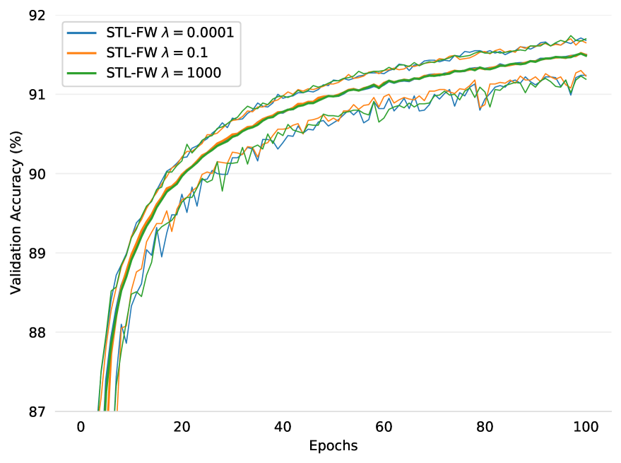
MNIST

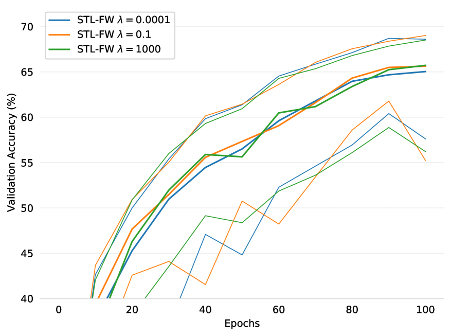
CIFAR10

Figure 3: Effect of the hyperparameter $\lambda$ of STL-FW on the convergence speed of D-SGD with 100 nodes, $d_{max}=10$.

D.4 Impact of $d_{max}$ on STL-FW

Figure 4 shows on a single plot the impact of the communication budget $d_{max}$ of STL-FW on the convergence speed of D-SGD. The communication budget has a strong impact in both cases, with STL-FW providing the same convergence speed as fully-connected when $d_{max}=99$, but with some residual variance because some nodes end up wth less than 99 edges. Most of the benefits of STL-FW are obtained with the first 10 edges, with additional edges providing only marginal benefits compared to fully-connected. We thus chose to show all experiments of the main text with three budgets, a small $d_{max}=2$, a medium $d_{max}=5$, and a large budget $d_{max}=10$.

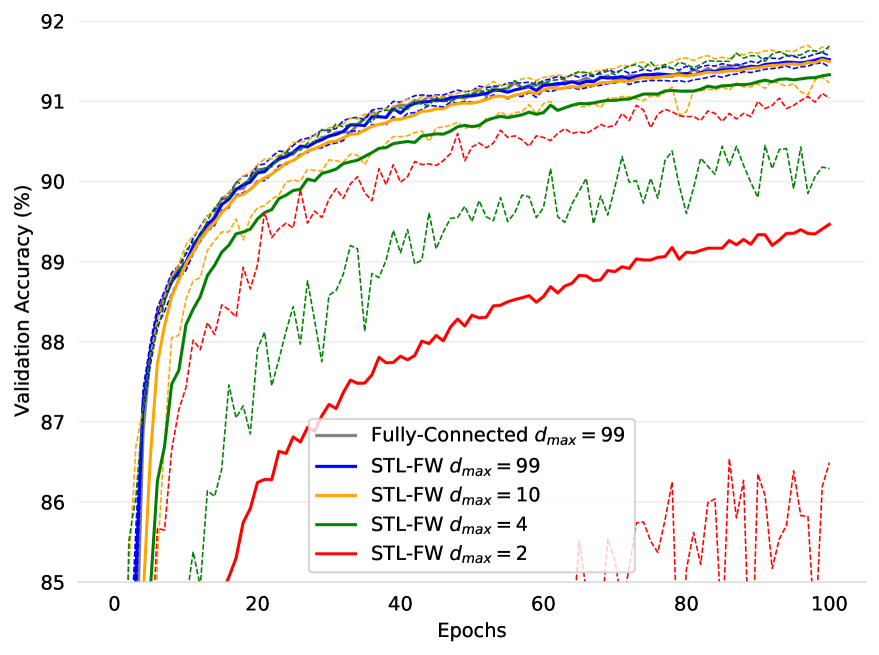
(a) MNIST

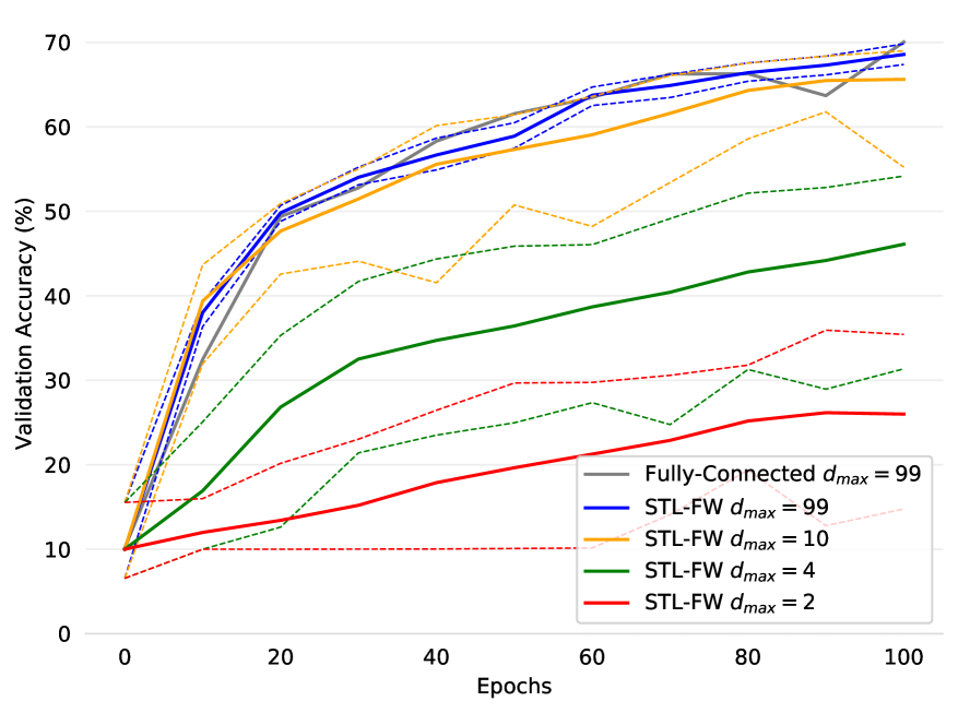
(b) CIFAR10

Figure 4: Effect of communication budget ($d_{max}$) of STL-FW on the convergence speed of D-SGD with 100 nodes, $\lambda=0.1$.

Finally, for a small budget $d_{max}=2$, we had seen in Figure 2 in the main text that STL-FW did not provide significant benefits compared to a random graph on CIFAR10. Figure 5 shows that as soon as $d_{max}=3$, STL-FW starts providing benefits compared to a random topology on CIFAR10.

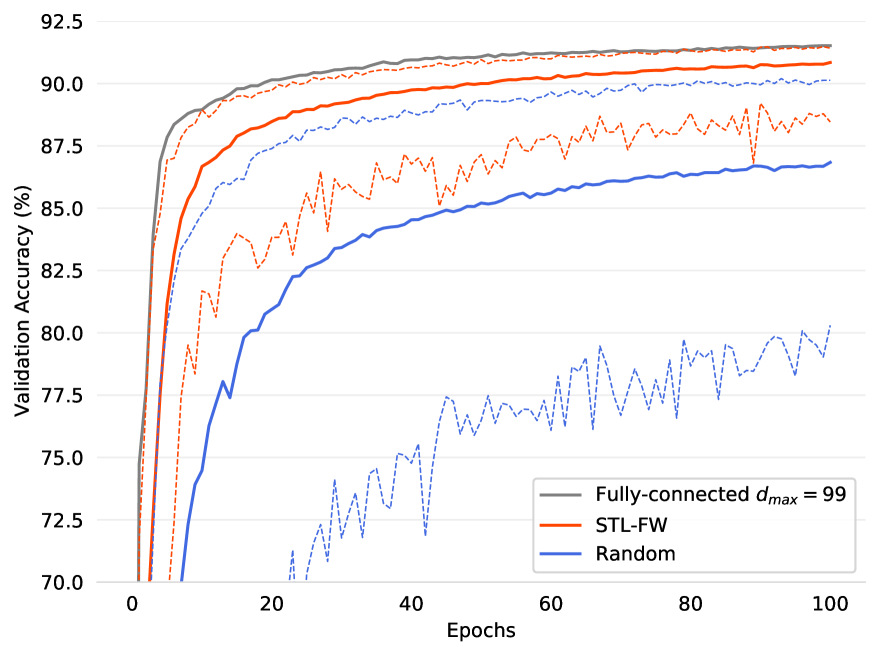
(a) MNIST

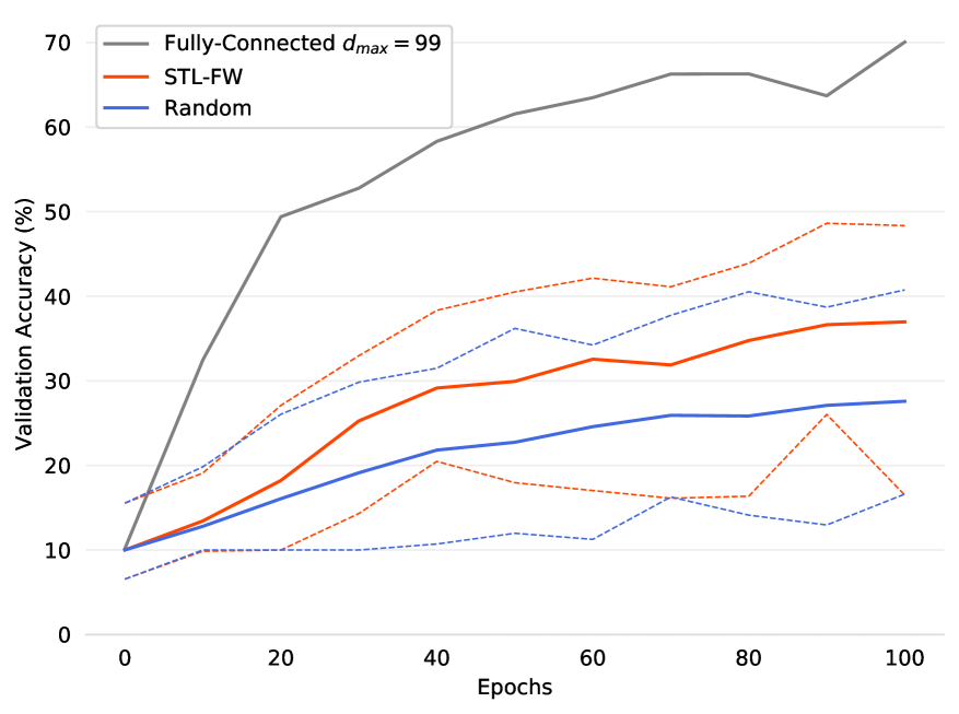
(b) CIFAR10

Figure 5: Convergence speed of D-SGD with our STL-FW topology and a random topology under small communication budget $d_{max}=3$.

References

- Assran et al., (2019) Assran, M., Loizou, N., Ballas, N., and Rabbat, M. (2019). Stochastic gradient push for distributed deep learning. In ICML.
- Bellet et al., (2022) Bellet, A., Kermarrec, A.-M., and Lavoie, E. (2022). D-Cliques: Compensating for Data Heterogeneity with Topology in Decentralized Federated Learning. In SRDS.
- Bottou et al., (2018) Bottou, L., Curtis, F. E., and Nocedal, J. (2018). Optimization methods for large-scale machine learning. Siam Review, 60(2):223–311.
- Boyd et al., (2004) Boyd, S., Diaconis, P., and Xiao, L. (2004). Fastest mixing markov chain on a graph. SIAM review, 46(4):667–689.
- Boyd et al., (2006) Boyd, S., Ghosh, A., Prabhakar, B., and Shah, D. (2006). Randomized gossip algorithms. IEEE Transactions on Information Theory, 52(6):2508–2530.
- Bubeck, (2014) Bubeck, S. (2014). Convex optimization: Algorithms and complexity. arXiv:1405.4980.
- Burkard et al., (2012) Burkard, R., Dell’Amico, M., and Martello, S. (2012). Assignment problems: revised reprint. SIAM.
- Chow et al., (2016) Chow, Y.-T., Shi, W., Wu, T., and Yin, W. (2016). Expander graph and communication-efficient decentralized optimization. In 2016 50th Asilomar Conference on Signals, Systems and Computers, pages 1715–1720. IEEE.
- Colin et al., (2016) Colin, I., Bellet, A., Salmon, J., and Clémençon, S. (2016). Gossip dual averaging for decentralized optimization of pairwise functions. In ICML.
- Crouse, (2016) Crouse, D. F. (2016). On implementing 2d rectangular assignment algorithms. IEEE Transactions on Aerospace and Electronic Systems, 52(4):1679–1696.
- Dandi et al., (2022) Dandi, Y., Koloskova, A., Jaggi, M., and Stich, S. U. (2022). Data-heterogeneity-aware mixing for decentralized learning. arXiv preprint arXiv:2204.06477.
- Dekel et al., (2012) Dekel, O., Gilad-Bachrach, R., Shamir, O., and Xiao, L. (2012). Optimal distributed online prediction using mini-batches. Journal of Machine Learning Research, 13(1).
- Deng, (2012) Deng, L. (2012). The mnist database of handwritten digit images for machine learning research. IEEE Signal Processing Magazine, 29(6):141–142. MNIST is distributed under Creative Commons Attribution-Share Alike 3.0 license.
- Esfandiari et al., (2021) Esfandiari, Y., Tan, S. Y., Jiang, Z., Balu, A., Herron, E., Hegde, C., and Sarkar, S. (2021). Cross-Gradient Aggregation for Decentralized Learning from Non-IID data. Technical report, arXiv:2103.02051.
- Even et al., (2022) Even, M., Massoulié, L., and Scaman, K. (2022). Sample Optimality and All-for-all Strategies in Personalized Federated and Collaborative Learning. Technical report, arXiv:2201.13097.
- Frank and Wolfe, (1956) Frank, M. and Wolfe, P. (1956). An algorithm for quadratic programming. Naval Research Logistics Quarterly, 3:95–110.
- Gao and Huang, (2020) Gao, H. and Huang, H. (2020). Periodic stochastic gradient descent with momentum for decentralized training. arXiv:2008.10435.
- Hsieh et al., (2020) Hsieh, K., Phanishayee, A., Mutlu, O., and Gibbons, P. B. (2020). The Non-IID Data Quagmire of Decentralized Machine Learning. In ICML.
- Huang and Pu, (2021) Huang, K. and Pu, S. (2021). Improving the transient times for distributed stochastic gradient methods. arXiv:2105.04851.
- Jaggi, (2013) Jaggi, M. (2013). Revisiting frank-wolfe: Projection-free sparse convex optimization. In ICML.
- Kairouz et al., (2021) Kairouz, P., McMahan, H. B., Avent, B., Bellet, A., et al. (2021). Advances and open problems in federated learning. Foundations and Trends® in Machine Learning, 14(1–2):1–210.
- Koloskova et al., (2021) Koloskova, A., Lin, T., and Stich, S. U. (2021). An improved analysis of gradient tracking for decentralized machine learning. NeurIPS, 34.
- Koloskova et al., (2020) Koloskova, A., Loizou, N., Boreiri, S., Jaggi, M., and Stich, S. U. (2020). A unified theory of decentralized sgd with changing topology and local updates. In ICML.
- Koloskova et al., (2019) Koloskova, A., Stich, S., and Jaggi, M. (2019). Decentralized stochastic optimization and gossip algorithms with compressed communication. In ICML.
- Kong et al., (2021) Kong, L., Lin, T., Koloskova, A., Jaggi, M., and Stich, S. (2021). Consensus control for decentralized deep learning. In ICML.
- Koppel et al., (2017) Koppel, A., Sadler, B. M., and Ribeiro, A. (2017). Proximity without consensus in online multiagent optimization. IEEE Transactions on Signal Processing, 65(12):3062–3077.
- Krizhevsky et al., (2009) Krizhevsky, A., Hinton, G., et al. (2009). Learning multiple layers of features from tiny images. CIFAR is distributed under MIT license.
- Li et al., (2019) Li, X., Yang, W., Wang, S., and Zhang, Z. (2019). Communication-efficient local decentralized sgd methods. arXiv:1910.09126.
- Lian et al., (2017) Lian, X., Zhang, C., Zhang, H., Hsieh, C.-J., Zhang, W., and Liu, J. (2017). Can decentralized algorithms outperform centralized algorithms? a case study for decentralized parallel stochastic gradient descent. NIPS.
- Lian et al., (2018) Lian, X., Zhang, W., Zhang, C., and Liu, J. (2018). Asynchronous Decentralized Parallel Stochastic Gradient Descent. In ICML.
- Lin et al., (2021) Lin, T., Karimireddy, S. P., Stich, S., and Jaggi, M. (2021). Quasi-global momentum: Accelerating decentralized deep learning on heterogeneous data. In ICML.
- Lovász and Plummer, (2009) Lovász, L. and Plummer, M. D. (2009). Matching theory, volume 367. American Mathematical Soc.
- Marfoq et al., (2021) Marfoq, O., Neglia, G., Bellet, A., Kameni, L., and Vidal, R. (2021). Federated Multi-Task Learning under a Mixture of Distributions. In NeurIPS.
- Marfoq et al., (2020) Marfoq, O., Xu, C., Neglia, G., and Vidal, R. (2020). Throughput-optimal topology design for cross-silo federated learning. NeurIPS.
- McMahan et al., (2017) McMahan, B., Moore, E., Ramage, D., Hampson, S., and y Arcas, B. A. (2017). Communication-efficient learning of deep networks from decentralized data. In AISTATS.
- Nedić et al., (2018) Nedić, A., Olshevsky, A., and Rabbat, M. G. (2018). Network topology and communication-computation tradeoffs in decentralized optimization. Proceedings of the IEEE, 106(5):953–976.
- Neglia et al., (2020) Neglia, G., Xu, C., Towsley, D., and Calbi, G. (2020). Decentralized gradient methods: does topology matter? In AISTATS.
- Nguyen et al., (2019) Nguyen, L. M., Nguyen, P. H., Richtárik, P., Scheinberg, K., Takác, M., and van Dijk, M. (2019). New convergence aspects of stochastic gradient algorithms. Journal of Machine Learning Research, 20:176–1.
- Stich and Karimireddy, (2020) Stich, S. U. and Karimireddy, S. P. (2020). The error-feedback framework: Better rates for sgd with delayed gradients and compressed updates. Journal of Machine Learning Research, 21:1–36.
- Sun et al., (2021) Sun, T., Li, D., and Wang, B. (2021). Stability and generalization of decentralized stochastic gradient descent. In Proceedings of the AAAI Conference on Artificial Intelligence, volume 35, pages 9756–9764.
- Tang et al., (2018) Tang, H., Lian, X., Yan, M., Zhang, C., and Liu, J. (2018). D²: Decentralized training over decentralized data. In ICML.
- Tewari et al., (2011) Tewari, A., Ravikumar, P., and Dhillon, I. (2011). Greedy algorithms for structurally constrained high dimensional problems. NIPS.
- Valls et al., (2020) Valls, V., Iosifidis, G., and Tassiulas, L. (2020). Birkhoff’s decomposition revisited: Sparse scheduling for high-speed circuit switches. arXiv:2011.02752.
- Vanhaesebrouck et al., (2017) Vanhaesebrouck, P., Bellet, A., and Tommasi, M. (2017). Decentralized collaborative learning of personalized models over networks. In AISTATS.
- Vogels et al., (2022) Vogels, T., Hendrikx, H., and Jaggi, M. (2022). Beyond spectral gap: The role of the topology in decentralized learning. arXiv preprint arXiv:2206.03093.
- Wang et al., (2019) Wang, J., Sahu, A. K., Yang, Z., Joshi, G., and Kar, S. (2019). Matcha: Speeding up decentralized sgd via matching decomposition sampling. In ICC.
- Ying et al., (2021) Ying, B., Yuan, K., Chen, Y., Hu, H., Pan, P., and Yin, W. (2021). Exponential graph is provably efficient for decentralized deep training. NeurIPS, 34.
- Yuan and Alghunaim, (2021) Yuan, K. and Alghunaim, S. A. (2021). Removing data heterogeneity influence enhances network topology dependence of decentralized sgd. arXiv:2105.08023.
- Yuan et al., (2020) Yuan, K., Alghunaim, S. A., Ying, B., and Sayed, A. H. (2020). On the influence of bias-correction on distributed stochastic optimization. IEEE Transactions on Signal Processing, 68:4352–4367.
- Yuan et al., (2021) Yuan, K., Chen, Y., Huang, X., Zhang, Y., Pan, P., Xu, Y., and Yin, W. (2021). Decentlam: Decentralized momentum sgd for large-batch deep training. In ICCV.
- Zantedeschi et al., (2020) Zantedeschi, V., Bellet, A., and Tommasi, M. (2020). Fully decentralized joint learning of personalized models and collaboration graphs. In AISTATS.
- Zhu et al., (2022) Zhu, T., He, F., Zhang, L., Niu, Z., Song, M., and Tao, D. (2022). Topology-aware generalization of decentralized sgd. In International Conference on Machine Learning, pages 27479–27503. PMLR.