Iterative Depth-First Search for Fully Observable Non-Deterministic Planning

Abstract

Fully Observable Non-Deterministic (fond) planning models uncertainty through actions with non-deterministic effects. Existing fond planning algorithms are effective and employ a wide range of techniques. However, most of the existing algorithms are not robust for dealing with both non-determinism and task size. In this paper, we develop a novel iterative depth-first search algorithm that solves fond planning tasks and produces strong cyclic policies. Our algorithm is explicitly designed for fond planning, addressing more directly the non-deterministic aspect of fond planning, and it also exploits the benefits of heuristic functions to make the algorithm more effective during the iterative searching process. We compare our proposed algorithm to well-known fond planners, and show that it has robust performance over several distinct types of fond domains considering different metrics.

Introduction

Fully Observable Non-Deterministic (fond) planning is an important planning model that aims to handle the uncertainty of the effects of actions (Cimatti et al. 2003). In fond planning, states are fully observable and actions may have non-deterministic effects (i.e., an action may generate a set of possible successor states). fond planning is relevant for solving other related planning models, such as stochastic shortest path (SSP) planning (Bertsekas and Tsitsiklis 1991), planning for temporally extended goals (Patrizi, Lipovetzky, and Geffner 2013; Camacho et al. 2017; Camacho and McIlraith 2019; Camacho et al. 2018; De Giacomo and Rubin 2018; Brafman and De Giacomo 2019), and generalized planning (Hu and Giacomo 2011; Bonet et al. 2017, 2020). Solutions for fond planning can be characterized as strong policies which guarantee to achieve the goal condition in a finite number of steps, and strong cyclic policies which guarantee to lead only to states from which a goal condition is satisfiable in a finite number of steps (Cimatti et al. 2003).

Existing fond planning algorithms in the literature are based on a diverse set of techniques and effectively solve difficult tasks when the non-determinism of the actions must be addressed. Cimatti et al. (2003) and Kissmann and Edelkamp (2009) have introduced model-checking planners based on binary decision diagrams. Some of the most effective fond planners rely on standard Classical Planning techniques by enumerating plans for a deterministic version of the task until producing a strong cyclic policy (Kuter et al. 2008; Fu et al. 2011; Muise, McIlraith, and Beck 2012; Muise, McIlraith, and Belle 2014; Muise, Belle, and McIlraith 2014). There are also planners that efficiently employ AND/OR heuristic search for solving fond planning tasks, such as myND (Mattmüller et al. 2010) and grendel (Ramírez and Sardiña 2014). Recently, Geffner and Geffner (2018) have proposed a SAT encoding for fond planning, and an iterative SAT-based planner that effectively handles the uncertainty of fond planning. Nevertheless, these fond planners present some limitations. Some of these planners address the non-determinism of the actions more indirectly, whereas others rely on algorithms with sophisticated and costly control procedures, and others do not take advantage of fundamental characteristics of planning models. As a result, such fond planners are not robust for dealing with some of the non-determinism aspects of fond planning and task size.

In this paper, we introduce a novel iterative depth-first search algorithm that solves fond planning tasks and produces strong cyclic policies. Our algorithm is based on two main concepts: (1) it is explicitly designed for solving fond planning tasks, so it addresses more directly the non-deterministic aspect of fond planning during the searching process; and (2) it exploits the benefits of heuristic functions to make the iterative searching process more effective. We also introduce an efficient version of our algorithm that prunes unpromising states in each iteration. To better understand the behavior of our proposed iterative depth-first search algorithm, we characterize its behavior through fundamental properties of fond planning policies.

We empirically evaluate our algorithm over two fond benchmark sets: a set from IPC (Bryce and Buffet 2008) and (Muise, McIlraith, and Beck 2012); and a set containing new fond planning domains, proposed by Geffner and Geffner (2018). We show that our algorithm outperforms some of the existing state-of-the-art fond planners on planning time and coverage, especially for the new fond domains. We also show that the pruning technique makes our algorithm competitive with existing fond planners. Our contributions open new research directions in fond planning, such as the design of more informed heuristic functions, and the development of more effective search algorithms.

Background

fond Planning

A Fully Observable Non-Deterministic (fond) planning task (Mattmüller et al. 2010) is a tuple $\Pi=\langle\mathcal{V},s_{0},s_{*},\mathcal{A}\rangle$. $\mathcal{V}$ is a set of state variables, and each variable $v\in\mathcal{V}$ has a finite domain $\textsc{D}_{v}$. A partial state $s$ maps variables $v\in\mathcal{V}$ to values in $\textsc{D}_{v}$, $s[v]\in\textsc{D}_{v}$, or to a undefined value $s[v]=\perp$. $\mathit{vars}(s)$ is the set of variables in $s$ with defined values. If every variable $\mathcal{V}$ in $s$ is defined, then $s$ is a state. $s_{0}$ is a state representing the initial state, whereas $s_{*}$ is a partial state representing the goal condition. A state $s$ is a goal state if and only if $s\models s_{*}$. $\mathcal{A}$ is a finite set of non-deterministic actions, in which every action $a\in\mathcal{A}$ consists of $a=\langle\emph{pre},\textsc{EFFS}\rangle$, where $\emph{pre}(a)$ is a partial state called preconditions, and $\textsc{EFFS}(a)$ is a non-empty set of partial states that represent the possible effects of $a$. A non-deterministic action $a\in\mathcal{A}$ is applicable in a state $s$ iff $s\models\emph{pre}(a)$. The application of an effect $\mathit{eff}\in\textsc{EFFS}(a)$ to a state $s$ generates a state $s^{\prime}=\textsc{succ}(s,\mathit{eff})$ with $s^{\prime}[v]=\mathit{eff}[v]$ if $v\in\mathit{vars}(\mathit{eff})$, and $s^{\prime}[v]=s[v]$ if not. The application of $\textsc{EFFS}(a)$ to a state $s$ generates a set of successor states $\textsc{SUCCS}(s,a)=\{\textsc{succ}(s,\mathit{eff})~{}\mid\mathit{eff}\in\textsc{EFFS}(a)\}$. We call $a\in\mathcal{A}$ simple deterministic if $|\textsc{EFFS}(a)|$ has size one.

A solution to a fond planning task $\Pi$ is a policy $\pi$ which is formally defined as a partial function $\pi:\mathcal{S}\mapsto\mathcal{A}\cup\{\perp\}$, which maps non-goal states of $\mathcal{S}$ into actions, such that an action $\pi(s)$ is applicable in the state $s$. A $\pi$-trajectory with length $k-1$ is a non-empty sequence of states $\langle s^{1},s^{2},\dots s^{k}\rangle$, such that $s^{i+1}\in\textsc{SUCCS}(s^{i},\pi(s^{i})),\forall i\in\{1,2,\dots,k-1\}$. A $\pi$-trajectory is called empty if it has a single state, and thus length zero. A policy $\pi$ is closed if any $\pi$-trajectory starting from $s_{0}$ ends either in a goal state or in a state defined in the policy $\pi$. A policy $\pi$ is a strong policy for $\Pi$ if it is closed and no $\pi$-trajectory passes through a state more than once. A policy $\pi$ is a strong cyclic policy for $\Pi$ if it is closed and any $\pi$-trajectory starting from $s_{0}$ which does not end in a goal state, ends in a state $s^{\prime}$ such that exists another $\pi$-trajectory starting from $s^{\prime}$ ending in a goal state. Note that a strong cyclic policy may re-visit states infinite times, in a cyclic way, but the fairness assumption guarantees that it will almost surely reach a goal state at some point along the execution. The assumption of fairness defines that all action outcomes in a given state will occur infinitely often (Cimatti et al. 2003).

Determinization and Heuristics for fond Planning

A determinization of a fond planning task $\Pi$ defines a new fond planning task $\Pi^{\textsc{Det}}$ where all actions are deterministic. Formally, $\Pi^{\textsc{Det}}=\langle\mathcal{V},s_{0},s_{*},\mathcal{A}^{\textsc{Det}}\rangle$ is a task where $\mathcal{A}^{\textsc{Det}}$ is a set of deterministic actions with one action $a^{\prime}$ for each outcome $\mathit{eff}\in\textsc{EFFS}(a)$ of all actions in $a\in\mathcal{A}$. A $s$-plan for $\Pi^{\textsc{Det}}$ is a sequence of actions that when applied to $s$ reaches a goal state. A $s$-plan is optimal if it has minimum cost among all $s$-plans. A solution for $\Pi^{\textsc{Det}}$ is a $s_{0}$-plan.

A heuristic function $h:\mathcal{S}\mapsto\mathbb{R}\cup\{\infty\}$ maps a state $s$ to its $h$-value, an estimation of the cost of a $s$-plan. A perfect heuristic $h^{*}$ maps a state $s$ to its optimal cost plan or $\infty$, if no plan exists. A heuristic is admissible if $h(s)\leq h^{*}(s)$ for all $s\in\mathcal{S}$. Delete-relaxation heuristics (Bonet and Geffner 2001; Hoffmann and Nebel 2001) can be efficiently used in fond planning by applying determinization (Mattmüller 2013). Other types of heuristics for fond planning have been proposed in the literature, such as pattern-database heuristics (Mattmüller et al. 2010), and pruning techniques (Winterer, Wehrle, and Katz 2016; Winterer et al. 2017).

fond Planners

One of the first fond planners in the literature was developed by Cimatti et al. (2003), and it is called mbp (Model-Based Planner). mbp solves fond planning tasks via model-checking, and it is built upon binary decision diagrams (BDDs). gamer (Kissmann and Edelkamp 2009), the winner of the fond track at IPC (2008), is also based on BDDs, but gamer has shown to be much more efficient than mbp.

myND (Mattmüller et al. 2010) is a fond planner based on an adapted version of LAO^∗ (Hansen and Zilberstein 2001), a heuristic search algorithm that has theoretical guarantees to extract strong cyclic solutions for Markov decision problems. ndp (Kuter et al. 2008) makes use of Classical Planning algorithms to solve fond planning tasks. fip (Fu et al. 2011) is similar to ndp, but the main difference is that fip avoids exploring already explored/solved states, being more efficient than ndp. prp (Muise, McIlraith, and Beck 2012) is one the most efficient fond planners in the literature, and it is built upon some improvements over the state relevance techniques, such as avoiding dead-ends states. The main idea of these planners is selecting a reachable state $s$ by the current policy that still is undefined in the current policy. Then, the planner finds a $s$-plan with $\Pi^{\textsc{Det}}$ and incorporates the $s$-plan into the policy. The planner repeats this process until the policy is strong cyclic, or it finds out that it is not possible to produce a strong cyclic policy from the current policy, and then it backtracks. Since these planners find $s$-plan for $\Pi^{\textsc{Det}}$ which do not consider the non-deterministic effects, they can take too much time to find that the current policy can not become a strong cyclic policy, or they can add actions to a policy that require too much search effort to become a strong cyclic policy.

grendel (Ramírez and Sardiña 2014) is a fond planner that combines regression with a symbolic fixed-point computation for extracting strong cyclic policies. Most recently, Geffner and Geffner (2018) developed fondsat, an iterative SAT-based fond planner that is capable to produce strong and strong cyclic policies for fond planning tasks.

Iterative Depth-First Search Algorithm
for fond Planning

In this section, we propose a novel iterative depth-first search algorithm called idfs that produces strong cyclic policies for fond planning tasks. idfs performs a series of bounded depth-first searches that consider the non-determinism aspect of fond planning during the iterative searching process. idfs produces a strong cyclic policy in a bottom-up way and only adds an action to the policy if it determines that the resulting policy with the additional action has the potential to become a strong cyclic policy without exceeding the current search- depth bound.

Evaluation Function $\mathcal{F}$

A heuristic function $h(s)$ estimates the length of a trajectory from the state $s$ to any goal state. It can assess whether a search procedure can reach a goal state without exceeding a search-depth bound. We define the $f$-value of a state $s$ as $f(s)=g(s)+h(s)$, with $g(s)$ being the search depth from $s_{0}$ to $s$. In this paper, we assume that all actions have a uniform action cost equal to one. During the iterative searching process, idfs considers the application of an action $a\in\mathcal{A}$ to a state $s$ by evaluating the set of generated successor states $\textsc{SUCCS}(s,a)$ using an evaluation function $\mathcal{F}_{\xi}$, which returns the estimate of the search depth required to reach a goal state through $\textsc{SUCCS}(s,a)$. The evaluation function $\mathcal{F}_{\xi}$ uses a parameter function $\xi$ to aggregate the $f$-values of states in $\textsc{SUCCS}(s,a)$: $\mathcal{F}_{\min}(\textsc{SUCCS}(s,a))$ is $\min_{s^{\prime}\in\textsc{SUCCS}(s,a)}f(s^{\prime})$, and $\mathcal{F}_{\max}(\textsc{SUCCS}(s,a))$ is $\max_{s^{\prime}\in\textsc{SUCCS}(s,a)}f(s^{\prime})$. Note that the evaluation function $\mathcal{F}_{\xi}$ is “pessimistic” when $\xi=\max$, whereas it is “optmistic” when $\xi=\min$.

The idfs Algorithm

We now present the idfs, and Algorithm 1 formally shows its pseudo-code.

// Main Iterative Loop.

1 idfs($s_{0}$):

2     $\mathit{bound}\coloneqq h(s_{0}),\mathit{nextBound}\coloneqq\infty$

3     while $\mathit{bound}\leq|\mathcal{S}|$ do

4         $\mathit{flag},\pi\coloneqq\textnormal{{\sc idfs${}_{R}$}}(s_{0},\emptyset,\emptyset,\emptyset)$

5         if $\mathit{flag}=\textsc{solved}$ then

6             return $\pi$

7        $\mathit{bound}\coloneqq\mathit{nextBound},\mathit{nextBound}\coloneqq\infty$

8    return unsolvable

// Recursion.

9 idfs_R($s,\mathscr{Z},\mathscr{Z}_{*},\pi$):

     // Base Cases.

10     if $s\models s_{*}$ or $\pi(s)\neq\bot$ or $s\in\mathscr{Z}_{*}$ then

11         return $\textsc{solved},\pi$]

12    if $s\in(\mathscr{Z}\setminus\mathscr{Z}_{*})$ then

13         return $\textsc{unsolved},\pi$

    // Evaluate Actions.

14     for $a\in\textsc{ApplicableActions}(s)$ do

15         if $\mathcal{F}_{\xi}(\textsc{SUCCS}(s,a))>\mathit{bound}$ and $\mathscr{Z}_{*}=\emptyset$ then

16             $\mathit{nextBound}\coloneqq\min\{\mathit{nextBound},\mathcal{F}_{\xi}(\textsc{SUCCS}(s,a))\}$

             continue // Next action.

17            

18        if $g(s)+1>\mathit{bound}$ then

19             $\mathit{nextBound}\coloneqq\min\{\mathit{nextBound},g(s)+1\}$

             continue // Next action.

20            

        // Fixed Point.

21         $\mathscr{Z}_{*}^{\prime}\coloneqq\mathscr{Z}_{*},\pi^{\prime}\coloneqq\pi,\mathscr{M}\coloneqq\textsc{SUCCS}(s,a),\mathscr{M}_{*}\coloneqq\emptyset$

22         repeat

23             $\textsc{reachedFixedPoint}\coloneqq\textsc{true}$

24             for $s^{\prime}\in(\mathscr{M}\setminus\mathscr{M}_{*})$ do

25                 $\mathit{flag},\pi^{\prime}\coloneqq\textnormal{{\sc idfs${}_{R}$}}(s^{\prime},\mathscr{Z}\cup\{s\},\mathscr{Z}_{*}^{\prime},\pi^{\prime})$

26                 if $\mathit{flag}=\textsc{solved}$ then

27                     $\mathscr{M}_{*}\coloneqq\mathscr{M}_{*}\cup\{s^{\prime}\}$

28                     $\mathscr{Z}_{*}^{\prime}\coloneqq\mathscr{Z}\cup\{s\}$

29                     $\textsc{reachedFixedPoint}\coloneqq\textsc{false}$

30                    

31                

32            

33        until reachedFixedPoint

34        if $\mathscr{M}_{*}=\mathscr{M}$ then

35             $\pi^{\prime}(s)\coloneqq a$

36             return $\textsc{solved},\pi^{\prime}$

37        

38    return $\textsc{unsolved},\pi$

Algorithm 1 idfs

Main Iterative Loop (Lines 1-8)

idfs performs a series of bounded depth-first searches, called iterations to solve a fond planning task $\Pi$. idfs assumes that $h$ is a heuristic function for the deterministic version of the task $\Pi$. Prior to the first iteration, idfs initializes the bound with the estimated value of heuristic function $h$ of the initial state $s_{0}$. At each iteration, idfs aims to produce a solution by searching to a depth of at most bound. The main loop receives a flag indicating if the iteration produced a solution from state $s_{0}$. If the flag is solved, then $\pi$ is a strong cyclic policy for task $\Pi$, and idfs returns it. If the flag is unsolved, then idfs_R could not produce a strong cyclic policy for task $\Pi$ with the current bound. Thus, idfs assigns to $\mathit{bound}$ the value of the global variable $\mathit{nextBound}$. The value of $\mathit{nextBound}$ is the minimum estimate ($\mathcal{F}_{\xi}$ or $g$-value$+1$) of a generated but not expanded set of successors. If no set of successors with a greater estimate than $\mathit{bound}$ is generated, the main loop returns unsolvable. This general strategy of depth-first search bounded by estimates is inspired by the Iterative Deepening A^∗ algorithm by Korf (1985).

Recursion (Lines 9-34)

idfs iteratively tries to produce a strong cyclic policy for task $\Pi$ in a bottom-up way, using a recursive procedure called idfs_R. Definition 1 formally defines the concept of partial strong cyclic policy, which we use to explain the behavior of idfs.

Definition 1.

A policy $\pi$ is a partial strong cyclic policy from a state $s$ of a fond task $\Pi$ for a set $A$ of primary target states and a set $B$ of secondary target states, iff $A$ is reachable from $s$ in $\pi$, and $\pi$ is sinking to $B$. (We omit $A$ and $B$, when the context is clear.)

• $A$ is reachable from $s$ in $\pi$ iff $s\in A$ or there is a $\pi$-trajectory starting from $s$ ending in a state of $A$ that does not includes a state of $B\setminus A$.

• $\pi$ is sinking to $B$ iff any $\pi$-trajectory either goes through a state of $B$ or ends in a state $s^{\prime}$, such that exists another $\pi$-trajectory starting from $s^{\prime}$ ending in a state of $B$.

idfs_R aims to produce a partial strong cyclic policy from state $s$ of a fond task $\Pi$ by searching to a depth of at most the current $\mathit{bound}$. idfs_R takes as input four arguments: the state $s$, the set $\mathscr{Z}$, the set $\mathscr{Z}_{*}$, and a policy $\pi$. These arguments are set to empty in each iteration of the main iterative loop. The set $\mathscr{Z}$ contains the ancestors of state $s$. The policy $\pi$ is the policy that idfs has built up to the moment of the current call of idfs_R. The set $\mathscr{Z}_{*}\subseteq\mathscr{Z}$ contains all ancestors of state $s$ that: are not in $\pi$ and are ancestors of states in $\pi$. Note that, in this case, idfs has found a trajectory to a goal state for all states in $\mathscr{Z}_{*}$. If idfs_R returns solved, then the returned policy is a partial strong cyclic policy from state $s$. The sets $A$ and $B$ of the partial strong cyclic policy are $A=\mathcal{S}_{*}\cup\mathcal{S}_{\pi}\cup\mathscr{Z}_{*}$ (primary target states) and the set $B=A\cup\mathscr{Z}$ (secondary target states). $\mathcal{S}_{\pi}$ is the set $\{s\mid\pi(s)\neq\bot\}$, and $\mathcal{S}_{*}$ the set $\{s\mid s\models s_{*}\}$ of goal states. Since $A=B=\mathcal{S}_{*}$ in the call of idfs_R in the main loop, the returned partial strong cyclic policy from state $s_{0}$ is a strong cyclic policy for task $\Pi$.

Consider the fond planning task example of Figure 1, in which, $s_{0}$ is the initial state, $s_{5}$ is the only goal state, and there are three non-deterministic actions, applied in states $s_{1},s_{3}$ and $s_{10}$. In the example, the current call of idfs_R is evaluating the state $s_{10}$ (with the current recursion path is in bold). In this call, the received policy $\pi$ contains the states $s_{2}$, $s_{3}$, $s_{4}$, $s_{6}$ and $s_{8}$ (in purple), i.e., $\mathcal{S}_{\pi}=\{s_{2},s_{3},s_{4},s_{6},s_{8}\}$. The ancestors of state $s_{10}$ are the states $s_{0}$, $s_{1}$ and $s_{9}$, i.e., $\mathscr{Z}=\{s_{0},s_{1},s_{9}\}$. The former two are in $\mathscr{Z}_{*}=\{s_{0},s_{1}\}$ (in green). Thus, the set $B$ of secondary target states includes states of $A$ and the state $s_{9}$.

idfs_R Base Cases (Lines 10-13)

idfs_R first checks whether the current state $s$ of the recursion is either a primary target state ($s\models s_{*}$ or $s\in\mathscr{Z}_{*}$ or $\pi(s)\neq\bot$), or a state $s\in\mathscr{Z}$ which is not primary target state. If the first case occurs, idfs_R returns solved. If the second case occurs, it returns unsolved. Both cases return policy unmodified.

idfs_R Evaluate Actions (Lines 14-20)

If the base cases do not address the state $s$, idfs_R proceeds to attempt to solve it (Line 14). To optimize the search, idfs_R evaluates first the applicable actions with least $\mathcal{F}_{\max}(\textsc{SUCCS}(s,a))$ and discards actions with $\mathcal{F}_{\max}(\textsc{SUCCS}(s,a))=\infty$. If the estimated solution depth of the successor states $\textsc{SUCCS}(s,a)$ is greater than the current $\mathit{bound}$ (i.e., $\mathcal{F}_{\xi}(\textsc{SUCCS}(s,a))>\mathit{bound}$) and $\mathscr{Z}_{*}=\emptyset$ (Line 15), then the set of successor states is discarded, and $\mathcal{F}_{\xi}(\textsc{SUCCS}(s,a))$ is assigned to $\mathit{nextBound}$ (Line 16) if $\mathit{nextBound}$ was greater than it.

idfs_R verifies whether $\mathscr{Z}_{*}=\emptyset$ because it aims to find at least one trajectory from $s$ to a primary target state in $A=\mathcal{S}_{*}\cup\mathcal{S}_{\pi}\cup\mathscr{Z}_{*}$. Note that $\mathcal{F}_{\xi}(\textsc{SUCCS}(s,a))$ aggregates $f$-values that only estimate the solution depth from $s_{0}$ through $\textsc{SUCCS}(s,a)$ to goal states. Thus, $\mathcal{F}_{\xi}(\textsc{SUCCS}(s,a))$ can only be used to estimate the solution depth to a primary target state when $\mathscr{Z}_{*}=\emptyset$, since it implies $A=\mathcal{S}_{*}$.

If $\mathscr{Z}_{*}\neq\emptyset$ the $g$-value the successor states $\textsc{SUCCS}(s,a)$ can be used to estimate the solution depth to a primary target state. In this case, if $g(n)+1$ is greater than the current $\mathit{bound}$, the set of successor states is discarded, and $g(n)+1$ is assigned to $\mathit{nextBound}$ if $\mathit{nextBound}$ was greater than it. If neither $\mathcal{F}_{\xi}(\textsc{SUCCS}(s,a))$ nor $g(s)$ prevent the search to proceed, idfs_R evaluates the successor states $\textsc{SUCCS}(s,a)$.

idfs_R Fixed Point (Lines 21-33)

Figure 1: Current path of analysis is in bold. Goal state in yellow. $\pi$ is in purple. $\mathscr{Z}_{*}$ is in green.

idfs_R recursively descends into the successor states $\textsc{SUCCS}(s,a)$ of $s$ to determine whether it should or not add the mapping $s\mapsto a$ to the police $\pi$. Namely, it adds the mapping $s\mapsto a$ to $\pi$ only if all the recursive calls on states of $\textsc{SUCCS}(s,a)$ returned solved (Lines 31–32). If not, it discards the possibility of using the action $a$ on $s$, and proceeds to the next action.

Consider again the fond planning task example of Figure 1. Assume that idfs_R reaches the point to evaluate the successor states $s_{11}$ and $s_{12}$ of $s_{10}$. Note that for $s_{10}$ the set of $A$ primary target states is $\{s_{0},s_{1},s_{2},s_{3},s_{4},s_{5},s_{6},s_{8}\}$, and the set $B$ of secondary target states is $\{s_{0},s_{1},s_{2},s_{3},s_{4},s_{5},s_{6},s_{8},s_{9}\}$. idfs_R aims to produce a policy $\pi^{\prime}$ such that $A$ is reachable from $s_{10}$ in $\pi^{\prime}$, and $\pi^{\prime}$ is sinking to $B$. To ensure that, idfs_R must find a trajectory from $s_{10}$ to a state in $A$ that does not include a state of $B\setminus A$. Thus, idfs_R analyzes all successors of $s_{10}$ to find such a trajectory. Before finding this trajectory, the arguments $\pi^{\prime}\coloneqq\pi$, $\mathscr{Z}^{\prime}\coloneqq\mathscr{Z}\cup\{s\}$ and $\mathscr{Z}_{*}^{\prime}\coloneqq\mathscr{Z}_{*}$ passed to idfs_R when evaluating states $s_{11}$ and $s_{12}$ remaining unchanged.

Suppose the first recursive call evaluates $s_{12}$, thus the primary targets states for $s_{12}$ are $A$. Since $s_{9}$ is an ancestor of $s_{12}$ and $s_{9}\notin A$, there is no trajectory from $s_{12}$ to a state of $A$ that does not includes a state of $B\setminus A$. Thus, the recursive call will fail and return unsolved. Next, idfs_R will proceed to the other successor state of $s_{10}$, namely $s_{11}$. If the recursive call on $s_{11}$ fails because of the bound, the algorithm will have analyzed all successors of $s_{10}$ without having any progress, as the set of successors states “already solved” $\mathscr{M}_{*}$ would not have changed, and thus a fixed-point would be reached, resulting in the action being discarded.

Suppose the recursive call on state $s_{11}$ does not fail, and it returns solved. Then, the returned policy is a partial strong cyclic policy from $s_{11}$ for the set of primary states $A^{\prime}$ and the set of secondary states $B^{\prime}$. Since $A^{\prime}=A$ and $B^{\prime}=B\cup\{s\}$. idfs_R now evaluates $s_{12}$ again, but now with a modified $A^{\prime}$. Since we already have a trajectory from $s_{10}$ to $A$, now $A^{\prime}$ includes also $s_{9},s_{10}$ and $s_{11}$, and $B^{\prime}=A^{\prime}$. The recursive call on $s_{12}$ returns solved because there is a trajectory to $A^{\prime}$. The new policy extended with $s_{10}\mapsto\mathbf{a}$ is a partial strong cyclic policy from $s_{10}$ for $A$ and $B$, and can be returned with the flag solved.

idfs_R End (Line 34)

In case none of the actions $a\in\textsc{ApplicableActions}(s)$ are able to generate a partial strong cyclic from $s$ to $A$ and $B$, idfs_R returns unsolved.

1

2

3idfsp($s_{0}$):

4     $\mathit{bound}\coloneqq h(s_{0}),\mathit{nextBound}\coloneqq\infty,\mathscr{X}\coloneqq\emptyset$

5     while $\mathit{bound}\leq|\mathcal{S}|$ do

6         $\mathit{flag},\pi\coloneqq\textnormal{{\sc idfsp${}_{R}$}}(s_{0},\emptyset,\emptyset,\emptyset)$

7         if $\mathit{flag}=\textsc{solved}$ then

8             return $\pi$

9        $\mathit{bound}\coloneqq\mathit{nextBound},\mathit{nextBound}\coloneqq\infty,\mathscr{X}\coloneqq\emptyset$

10    return unsolved

11

12idfsp_R($s,\mathscr{Z},\mathscr{Z}_{*},\pi$):

     $\leftarrow$  Lines 10-13 of Algorithm 1.

13    

14    if $s\in\mathscr{X}$ then

15         return $\textsc{unsolved},\pi$

16    

17    $\textsc{promising}\coloneqq\textsc{false}$

18     for $a\in\textsc{ApplicableActions}(s)$ do

         $\leftarrow$  Lines 15-20 of Algorithm 1.

         // Fixed Point.

19         $\mathscr{Z}_{*}^{\prime}\coloneqq\mathscr{Z}_{*},\pi^{\prime}\coloneqq\pi,\mathscr{M}\coloneqq\textsc{SUCCS}(s,a),\mathscr{M}_{*}\coloneqq\emptyset$

20         repeat

21             $\textsc{reachedFixedPoint}\coloneqq\textsc{true}$

22             for $s^{\prime}\in(\mathscr{M}\setminus\mathscr{M}_{*})$ do

23                 $\mathit{flag},\pi^{\prime}\coloneqq\textnormal{{\sc idfsp${}_{R}$}}(s^{\prime},\mathscr{Z}\cup\{s\},\mathscr{Z}_{*}^{\prime},\pi^{\prime})$

24                 if $\mathscr{M}\cap\mathscr{X}\neq\emptyset$ then

25                     break

26                    

27                if $\mathit{flag}=\textsc{solved}$ then

28                     $\mathscr{M}_{*}\coloneqq\mathscr{M}_{*}\cup\{s^{\prime}\}$

29                     $\mathscr{Z}_{*}^{\prime}\coloneqq\mathscr{Z}\cup\{s\}$

30                     $\textsc{reachedFixedPoint}\coloneqq\textsc{false}$

31                    

32                

33            if $\mathscr{M}\cap\mathscr{X}\neq\emptyset$ then

34                 break

35                

36            if reachedFixedPoint then

37                 $\textsc{promising}\coloneqq\textsc{true}$

38                

39            

40        until reachedFixedPoint

        $\leftarrow$  Lines 31-33 of Algorithm 1.

41        

42    if $\textsc{promising}=\textsc{false}$ then

43         $\mathscr{X}\coloneqq\mathscr{X}\cup\{s\}$

44        

45    return $\textsc{unsolved},\pi$

Algorithm 2 idfs Pruning (idfsp)

idfs Pruning

We now present an extended version of idfs called idfs Pruning (idfsp). Algorithm 2 presents the pseudo-code of idfsp. In essence, idfsp is similar to idfs, and the main difference is that it prunes states during the searching process. idfsp_R considers that a state $s$ is promising if $s\in A$ or at least one of its applicable actions $a$ reaches the fixed point when evaluating the set of successor states $\mathscr{M}\coloneqq\textsc{SUCCS}(s,a)$. If the state $s$ is not promising, idfsp_R adds the state $s$ into the global set $\mathscr{X}$. idfsp sets $\mathscr{X}$ to empty before each iteration. idfsp_R has one additional base case that returns unsolved if state $s\in\mathscr{X}$ (Lines 10–11). During the fixed-point computation, idfsp_R verifies if at least one of the states in $\mathscr{M}\coloneqq\textsc{SUCCS}(s,a)$ is in $\mathscr{X}$ and stops the fixed-point computation if it is. This pruning method helps the search because it avoids repeated evaluation of states that generate successors that can not be part of the policy with the current bound.

Minimal Critical-Value in fond Planning

We now introduce key properties about the set of strong cyclic policies of a fond task $\Pi$ that are important to characterize the behavior of idfs. A fond planning task $\Pi$ has a set of strong cyclic policies $\mathcal{P}(\Pi)$ – if $\Pi$ is unsolvable, then $\mathcal{P}(\Pi)=\emptyset$. Figure 2a shows the state-space of a fond planning task $\Pi$, with eight states, three deterministic actions, and two non-deterministic actions – namely $\{a,b\}$. This task has only two strong cyclic policies, $\pi_{0}=\{s_{0}\mapsto\mathbf{c},\break s_{4}\mapsto\mathbf{b},s_{5}\mapsto\mathbf{d},s_{6}\mapsto\mathbf{c},s_{7}\mapsto\mathbf{e}\}$ and $\pi_{1}=\{s_{0}\mapsto\mathbf{a},s_{2}\mapsto\mathbf{c},\break s_{3}\mapsto\mathbf{d}\}$. Figures 2b and 2c, show respectively the part of the state-space reachable from $s_{0}$ using each policy. We use these state-spaces to present the concept of critical-values of policies (Definition 2).

Definition 2.

The critical-value $\mathbf{cv}(\pi)$ of a policy $\pi$ is the value of the length of the longest $\pi$-trajectory $\langle s^{1},s^{2},\dots,s^{k}\rangle$ with $s^{1}=s_{0}$ and no $i<j\leq k-1$ with $s^{i}=s^{j}$.

The $\mathbf{cv}$ of $\pi_{0}$ is generated by $\langle s_{0},s_{4},s_{5},s_{6},s_{7},s_{4}\rangle$, therefore $\mathbf{cv}(\pi_{0})=5$. The $\mathbf{cv}$ of $\pi_{1}$ is generated by $\langle s_{0},s_{2},s_{3},s_{0}\rangle$, therefore $\mathbf{cv}(\pi_{1})=3$. Definition 3 introduces the concept of minimal critical-value $\mathbf{cv}^{*}$ of a fond planning task $\Pi$.

Definition 3.

The minimal critical-value $\mathbf{cv}^{*}$ of a fond planning task $\Pi$ is equal to $\min_{\pi\in\mathcal{P}(\Pi)}\mathbf{cv}(\pi)$.

Figure 2: Minimal Critical-Value example.

(a)
(b) (c)

Thus, the $\mathbf{cv}^{*}$ of the fond planning task $\Pi$ in the Figure 2a is $\mathbf{cv}^{*}(\Pi)=\min\{\mathbf{cv}(\pi_{0}),\mathbf{cv}(\pi_{1})\}=\min\{5,3\}=3$. Definition 3 considers all strong cyclic policies of the task $\Pi$, which are, in general, unavailable. Therefore, we usually do not know the value of $\mathbf{cv}^{*}(\Pi)$. Nevertheless, we prove that if idfs uses $\mathcal{F}_{\min}$ and an admissible heuristic function for the deterministic version of the task $\Pi$, idfs will search to a depth of at most $\mathbf{cv}^{*}$. Thus, if $\Pi$ is solvable, idfs will return a strong cyclic policy before the search starts evaluating states at a depth greater than $\mathbf{cv}^{*}$.

	idfs ($\mathcal{F}_{\min}$, $\mathit{h}^{\textsc{blind}}$)						idfs ($\mathcal{F}_{\min}$, $\mathit{h}^{\textsc{max}}$)
Domain (#)	C	T	$|\pi|$	$b_{I}$/$b_{F}$	$i$		C	T	$|\pi|$	$b_{I}$/$b_{F}$	$i$
doors (#15)	11	30.1	1486.7	0.0/8.0	8.0		11	10.9	1486.7	7.0/8.0	2.0
islands (#60)	29	18.7	4.9	0.0/4.9	4.9		60	0.1	4.9	4.9/4.9	1.0
miner (#51)	0	-	-	-/-	-		40	-	-	-/-	-
tw-spiky (#11)	4	18.5	26.0	0.0/22.0	22.0		9	3.7	25.0	8.0/22.0	15.0
tw-truck (#74)	13	23.4	13.8	0.0/10.8	10.8		26	0.6	13.2	4.2/10.8	7.7
Sub-Total (#211)	57	22.6	382.5	0.0/11.4	11.4		146	3.8	382.4	6.1/11.4	6.4
acrobatics (#8)	4	2.3	14.0	0.0/14.0	14.0		8	0.1	14.0	3.8/14.0	11.3
beam-walk (#11)	8	29.2	254.0	0.0/254.0	254.0		8	9.5	254.0	127.5/254.0	127.5
bw-orig (#30)	10	17.4	13.5	0.0/7.5	7.5		10	4.2	12.4	2.8/7.5	5.7
bw-2 (#15)	5	38.0	14.4	0.0/9.4	9.4		5	4.9	14.2	2.8/9.4	7.6
bw-new (#40)	6	26.8	8.0	0.0/5.5	5.5		6	2.5	8.0	2.2/5.5	4.2
chain (#10)	2	62.8	42.0	0.0/28.0	28.0		10	0.1	42.0	28.0/28.0	1.0
earth-obs (#40)	8	3.9	19.3	0.0/9.6	9.6		9	0.4	18.3	4.4/9.6	6.0
elevators (#15)	4	44.0	12.0	0.0/11.3	11.3		5	1.5	11.3	4.8/11.3	7.5
faults (#55)	18	14.8	28.4	0.0/7.3	7.3		19	7.7	21.6	2.0/7.3	6.3
first-resp (#100)	20	22.5	5.7	0.0/5.7	5.7		23	3.7	6.3	2.6/5.7	4.0
tri-tw (#40)	3	23.2	22.0	0.0/15.0	15.0		3	13.4	22.0	4.0/15.0	12.0
zeno (#15)	0	-	-	-/-	-		3	-	-	-/-	-
Total (#590)	145	25.0	131.0	0.0/27.5	27.5		255	3.7	130.3	13.9/27.5	14.6

Table 1: idfs comparison with $\mathcal{F}_{\min}$: $\mathit{h}^{\textsc{blind}}$ vs $\mathit{h}^{\textsc{max}}$.

Theoretical Properties

In this section, we present a proof idea that shows that if a fond planning task $\Pi$ is solvable, idfs returns a strong cyclic policy by searching to a depth of at most $\mathbf{cv}^{*}(\Pi)$, and if $\Pi$ is unsolvable, idfs identifies it correctly. Theorem 1 bounds the behavior of the idfs algorithm by the structure of the fond planning task $\Pi$.

Theorem 1.

Given a fond planning task $\Pi$, an admissible heuristic function $h$ for a deterministic version of $\Pi$, and idfs using $\mathcal{F}_{\min}$. If $\Pi$ is solvable, then idfs returns a strong cyclic policy $\pi$ by searching to a depth of at most $\mathbf{cv}^{*}(\Pi)$. If $\Pi$ is unsolvable, then idfs returns unsolvable.

Proof Idea. If $\Pi$ is solvable, then there is a strong cyclic policy $\pi$ which has $\mathbf{cv}(\pi)=\mathbf{cv}^{*}(\Pi)$. Suppose state $s$ is part of the policy $\pi$, idfs_R analyzes all actions applicable on $s$, including the action that is part of the policy $\pi(s)$, with incremental search depths and using $\mathcal{F}_{\min}$ and heuristic $h$ when possible. Since $s$ is in the policy $\pi$, idfs_R can, by the construction of the algorithm, find a policy that includes $s$ searching to a depth of at most $\mathbf{cv}^{*}$. Because task $\Pi$ is solvable and $s_{0}$ is in any policy including policy $\pi$, idfs returns a strong cyclic policy by searching to a depth of at most $\mathbf{cv}^{*}$. idfs_R only returns solved for a state $s$ using action $a$ if all its successors in $\textsc{SUCCS}(s,a)$ return solved. Thus, if a fond planning task $\Pi$ is unsolvable, idfs returns unsolvable. idfs always terminates because the state-space size limits the number of iterations of the main loop.

Experiments and Evaluation

We now present the set of experiments we have conducted to evaluate the efficiency of our idfs algorithm for solving fond planning tasks. We compare our algorithm to state-of-the-art fond planners, such as prp (Muise, McIlraith, and Beck 2012), myND (Mattmüller et al. 2010), and fondsat (Geffner and Geffner 2018). We have implemented our algorithm using part of the source code of myND. We use the delete relaxation heuristic functions for the deterministic version of the planning task as proposed by Mattmüller (2013). As a result, we have a fond planner called paladinus .

We empirically evaluate idfs using two distinct benchmark sets: IPC-fond and NEW-fond. IPC-fond contains 379 planning tasks over 12 fond domains from the IPC (2008) and (Muise, McIlraith, and Beck 2012). The NEW-fond benchmark set (Geffner and Geffner 2018) introduces fond planning tasks that contain several trajectories to goal states that are not part of any strong cyclic policy. NEW-fond contains 211 tasks over five fond domains, namely doors, islands, miner, tw-spiky, and tw-truck. Note that 25 out of 590 tasks are unsolvable, namely, 25 fond planning tasks of first-resp– a domain of IPC-fond.

We have run all experiments using a single core of a 12 core Intel(R) Xeon(R) CPU E5-2620 v3 @ 2.40GHz with 16GB of RAM, with a memory limit of 4GB, and set a 5 minute (300 seconds) time-out per planning task. We evaluate the planners, when applicable, using the following metrics: number of solved tasks, i.e., coverage ($C$), time to solve ($T$) in seconds, average policy size ($|\pi|$), initial bound and the final bound (respectively, $b_{I}$ and $b_{F}$), and the number iterations ($i$). Apart from the coverage ($C$), all results shown in Tables 1, 2, 3, and 5 are calculated over the intersection of the tasks solved by all planners in the respective table.

idfs with Admissible Heuristic Functions

	idfs ($\mathcal{F}_{\min}$, $\mathit{h}^{\textsc{add}}$)						idfs ($\mathcal{F}_{\max}$, $\mathit{h}^{\textsc{add}}$)
Domain (#)	C	T	$|\pi|$	$b_{I}$/$b_{F}$	$i$		C	T	$|\pi|$	$b_{I}$/$b_{F}$	$i$
doors (#15)	11	14.1	1486.7	26.7/35.7	1.9		11	10.7	1486.7	26.7/120.5	2.8
islands (#60)	60	0.5	7.0	7.0/7.0	1.0		60	0.6	7.0	7.0/7.0	1.0
miner (#51)	51	1.1	23.2	39.6/39.9	1.2		51	1.8	23.2	39.6/39.9	1.2
tw-spiky (#11)	9	14.9	25.0	8.0/22.0	15.0		6	39.8	25.0	8.0/24.0	17.0
tw-truck (#74)	26	19.3	14.3	3.9/11.1	8.2		21	30.0	14.4	3.9/12.1	9.2
Sub-Total (#211)	157	9.9	311.2	17.1/23.1	5.4		149	16.6	311.2	17.1/40.7	6.2
acrobatics (#8)	8	1.6	126.5	63.8/126.5	63.8		8	0.6	126.5	63.8/748.1	73.9
beam-walk (#11)	11	0.5	453.2	453.2/453.2	1.0		9	12.0	453.2	453.2/39176.7	113.6
bw-orig (#30)	15	10.5	23.2	14.6/15.2	1.6		25	0.6	17.3	14.6/22.4	2.0
bw-2 (#15)	7	1.6	21.6	15.4/17.0	2.1		14	0.8	21.3	15.4/22.6	2.0
bw-new (#40)	10	3.3	20.0	12.3/12.8	1.4		19	0.6	17.4	12.3/19.3	2.0
chain (#10)	10	0.3	162.0	161.0/161.8	1.8		10	0.3	162.0	161.0/161.8	1.8
earth-obs (#40)	18	0.2	47.4	22.9/23.9	1.7		19	0.5	38.8	22.9/25.8	2.5
elevators (#15)	10	0.1	19.6	21.1/21.7	1.6		8	0.2	19.6	21.1/21.9	1.7
faults (#55)	22	19.5	26.8	5.9/7.9	3.0		23	16.2	26.8	5.9/9.1	2.6
first-resp (#100)	57	0.3	13.7	12.6/12.6	1.0		31	28.7	14.3	12.6/13.8	2.2
tri-tw (#40)	3	13.2	22.0	4.0/15.0	12.0		3	9.8	22.0	4.0/15.0	8.0
zeno (#15)	7	13.4	29.5	30.0/31.2	2.2		6	17.8	29.5	30.0/31.2	2.2
Total (#590)	335	6.7	148.3	53.1/59.7	7.1		324	10.1	147.4	53.1/2380.7	14.5

Table 2: idfs algorithm using $\mathit{h}^{\textsc{add}}$ with $\mathcal{F}_{\min}$ and $\mathcal{F}_{\max}$, without pruning.

	idfsp ($\mathcal{F}_{\min}$, $\mathit{h}^{\textsc{add}}$)						idfsp ($\mathcal{F}_{\max}$, $\mathit{h}^{\textsc{add}}$)
Domain (#)	C	T	$|\pi|$	$b_{I}$/$b_{F}$	$i$		C	T	$|\pi|$	$b_{I}$/$b_{F}$	$i$
doors (#15)	13	2.3	1486.7	26.7/35.7	1.9		13	1.7	1486.7	26.7/120.5	2.8
islands (#60)	60	0.3	7.0	7.0/7.0	1.0		60	0.5	7.0	7.0/7.0	1.0
miner (#51)	51	0.8	23.2	39.6/39.9	1.2		51	0.9	23.2	39.6/39.9	1.2
tw-spiky (#11)	10	2.5	1409.3	8.0/20.0	13.0		10	3.4	1409.3	8.0/22.0	15.0
tw-truck (#74)	55	0.2	17.4	3.9/12.8	9.9		44	2.1	19.8	3.9/17.3	14.4
Sub-Total (#211)	189	1.2	588.7	17.1/23.1	5.4		178	1.7	589.2	17.1/41.3	6.8
acrobatics (#8)	8	0.1	126.5	63.8/63.8	1.0		8	0.6	126.5	63.8/749.8	75.5
beam-walk (#11)	11	0.4	453.2	453.2/453.2	1.0		11	0.5	453.2	453.2/39176.7	113.6
bw-orig (#30)	16	7.5	23.8	14.6/17.6	3.9		29	0.3	16.9	14.6/22.6	2.2
bw-2 (#15)	10	1.0	17.4	15.4/18.6	3.4		15	0.3	19.1	15.4/22.9	2.3
bw-new (#40)	12	1.6	14.4	12.3/14.9	3.5		21	0.2	17.4	12.3/19.3	2.0
chain (#10)	10	0.3	162.0	161.0/161.8	1.8		10	0.3	162.0	161.0/161.8	1.8
earth-obs (#40)	19	1.4	40.9	22.9/28.1	4.3		25	0.1	35.6	22.9/27.9	3.9
elevators (#15)	9	0.1	19.4	21.1/21.7	1.6		8	0.1	19.4	21.1/21.9	1.7
faults (#55)	55	0.1	47.5	5.9/7.5	1.8		55	0.1	43.1	5.9/8.9	2.3
first-resp (#100)	60	0.3	19.7	12.6/12.6	1.1		46	5.9	109.5	12.6/13.8	2.3
tri-tw (#40)	36	0.1	26.0	4.0/13.3	10.3		8	0.1	22.0	4.0/15.0	8.0
zeno (#15)	6	12.8	29.7	30.0/31.2	2.2		8	12.9	29.7	30.0/31.2	2.2
Total (#590)	411	1.9	230.8	53.1/56.4	3.7		422	1.8	235.3	53.1/2381.1	14.8

Table 3: idfs algorithm using $\mathit{h}^{\textsc{add}}$ with $\mathcal{F}_{\min}$ and $\mathcal{F}_{\max}$, with pruning.

(a)

(b)

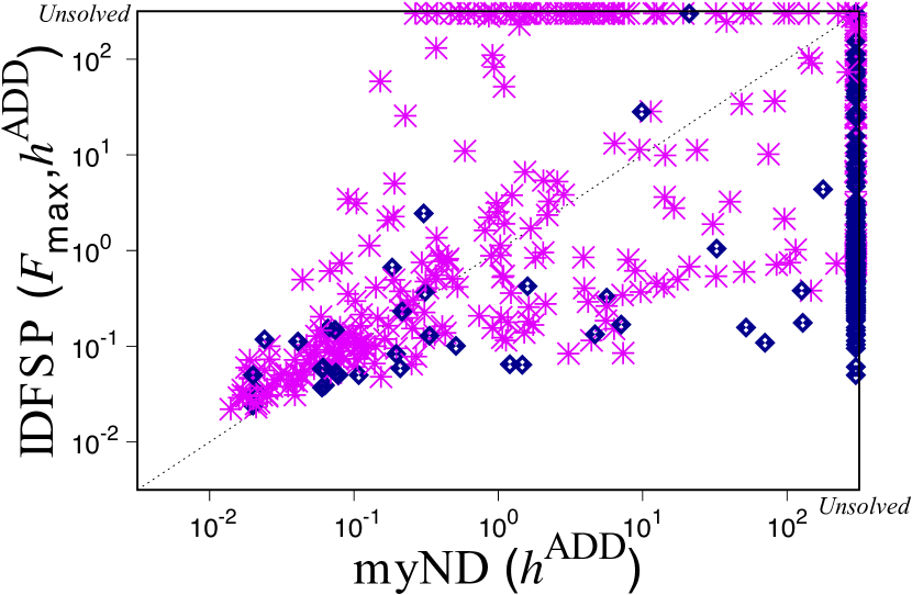
(c)

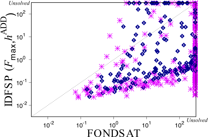
(d)

Figure 3: Planning time (in seconds) per planning task. Blue diamonds: results for the NEW-fond benchmark set; Dark-pink asterisks: results for the IPC-fond benchmark set.

We start our evaluation by presenting a comparison of idfs using $\mathit{h}^{\textsc{blind}}$ and $\mathit{h}^{\textsc{max}}$ with the evaluation function $\mathcal{F}_{\min}$. This comparison evaluates how useful the information of the heuristic function is for idfs concerning search efficiency. We evaluate this with the following metrics: the number of solved tasks, the time to solve, and the number of iterations required to solve the task – fewer iterations mean that idfs reaches faster the depth where it finds a strong cyclic policy. Table 1 summarizes the results for all 17 fond domains of the used benchmark sets, showing the performance of idfs when using $\mathcal{F}_{\min}$ with $\mathit{h}^{\textsc{max}}$ and $\mathit{h}^{\textsc{blind}}$, denoted as idfs ($\mathcal{F}_{\min}$, $\mathit{h}^{\textsc{max}}$) and idfs ($\mathcal{F}_{\min}$, $\mathit{h}^{\textsc{blind}}$), respectively.

idfs ($\mathcal{F}_{\min}$, $\mathit{h}^{\textsc{max}}$) solves in total 255 tasks, whereas idfs ($\mathcal{F}_{\min}$, $\mathit{h}^{\textsc{blind}}$) solves 145 tasks. Both idfs ($\mathcal{F}_{\min}$, $\mathit{h}^{\textsc{max}}$) and idfs ($\mathcal{F}_{\min}$, $\mathit{h}^{\textsc{blind}}$) identified the 25 tasks of first-resp as unsolvable. idfs ($\mathcal{F}_{\min}$, $\mathit{h}^{\textsc{blind}}$) exceeded the time limit to solve all tasks of miner and zeno. Table 1 shows that idfs ($\mathcal{F}_{\min}$, $\mathit{h}^{\textsc{max}}$) always uses fewer iterations to solve the same tasks when compared to idfs ($\mathcal{F}_{\min}$, $\mathit{h}^{\textsc{blind}}$), and it also shows that, in general, idfs ($\mathcal{F}_{\min}$, $\mathit{h}^{\textsc{max}}$) is much faster even considering the cost of computing the heuristic function.

Figure 3a shows the planning time comparison between idfs ($\mathcal{F}_{\min}$, $\mathit{h}^{\textsc{max}}$) and idfs ($\mathcal{F}_{\min}$, $\mathit{h}^{\textsc{blind}}$). Overall, idfs ($\mathcal{F}_{\min}$, $\mathit{h}^{\textsc{max}}$) outperforms idfs ($\mathcal{F}_{\min}$, $\mathit{h}^{\textsc{blind}}$) with respect to planning time among most planning tasks, especially over the NEW-fond benchmarks (blue diamond in Figure 3a). Thus, we conclude that, in general, idfs benefits from using the information of the heuristic function.

idfs vs. idfs Pruning

We now evaluate our idfs algorithm using $\mathit{h}^{\textsc{add}}$ with $\mathcal{F}_{\max}$ and $\mathcal{F}_{\min}$. We also compare the versions of idfs with and without pruning. Tables 2 and 3 show the results the four variations of idfs with $\mathit{h}^{\textsc{add}}$. Note that all four variations of idfs with $\mathit{h}^{\textsc{add}}$ solved more tasks than both idfs ($\mathcal{F}_{\min}$, $\mathit{h}^{\textsc{max}}$) and idfs ($\mathcal{F}_{\min}$, $\mathit{h}^{\textsc{blind}}$). Such empirical results show that using a more informative heuristic has a significant impact on the results. idfs ($\mathcal{F}_{\min}$, $\mathit{h}^{\textsc{add}}$) solved 80 tasks more than idfs ($\mathcal{F}_{\min}$, $\mathit{h}^{\textsc{max}}$). idfsp ($\mathcal{F}_{\max}$, $\mathit{h}^{\textsc{add}}$) outperforms the other variants in terms of coverage and planning time. However, the average final bound $b_{F}$, and the average number of iterations $i$ for the intersection of the solved tasks are higher for variations with $\mathcal{F}_{\max}$ compared to the variations with $\mathcal{F}_{\min}$. Also, the pruning variants (idfsp) are far superior to the variants without pruning.

Planner	Solved Tasks (#590)
paladinus idfsp ($\mathcal{F}_{\min}$, $\mathit{h}^{\textsc{max}}$)	337
paladinus idfsp ($\mathcal{F}_{\min}$, $\mathit{h}^{\textsc{ff}}$)	406
paladinus idfsp ($\mathcal{F}_{\min}$, $\mathit{h}^{\textsc{add}}$)	411
paladinus idfsp ($\mathcal{F}_{\max}$, $\mathit{h}^{\textsc{max}}$)	334
paladinus idfsp ($\mathcal{F}_{\max}$, $\mathit{h}^{\textsc{ff}}$)	380
paladinus idfsp ($\mathcal{F}_{\max}$, $\mathit{h}^{\textsc{add}}$)	422
fondsat	276
prp ($\mathit{h}^{\textsc{max}}$)	292
prp ($\mathit{h}^{\textsc{ff}}$)	412
prp ($\mathit{h}^{\textsc{add}}$)	389
myND ($\mathit{h}^{\textsc{max}}$)	180
myND ($\mathit{h}^{\textsc{ff}}$)	265
myND ($\mathit{h}^{\textsc{add}}$)	289

Table 4: Overall coverage results.

Comparison with other fond Planners

	idfsp ($\mathcal{F}_{\max}$, $\mathit{h}^{\textsc{add}}$)				prp ($\mathit{h}^{\textsc{ff}}$)				myND ($\mathit{h}^{\textsc{add}}$)				fondsat
Domain (#)	C	T	$|\pi|$		C	T	$|\pi|$		C	T	$|\pi|$		C	T	$|\pi|$
doors (#15)	13	0.34	670.0		12	0.13	16.0		9	6.77	670.0		10	23.48	16.0
islands (#60)	60	0.10	6.5		27	0.08	7.5		12	11.06	6.83		46	4.38	7.5
miner (#51)	51	-	-		9	-	-		0	-	-		28	-	-
tw-spiky (#11)	10	0.13	25.0		1	17.4	23.0		1	0.33	25.0		3	97.07	23.0
tw-truck (#74)	44	2.97	21.27		17	20.34	19.36		12	12.94	13.82		67	4.51	12.18
Sub-Total (#211)	178	0.88	180.69		66	9.49	16.47		36	7.77	178.91		154	32.36	14.67
acrobatics (#8)	8	0.05	8.33		8	9.43	9.33		8	0.02	8.33		3	3.04	9.33
beam-walk (#11)	11	0.02	11.0		11	0.86	12.0		10	0.02	11.0		2	1.37	12.0
bw-orig (#30)	29	0.10	12.2		30	0.06	11.7		15	0.10	11.6		10	15.02	11.1
bw-2 (#15)	15	0.12	13.2		15	0.08	14.4		6	0.23	17.6		5	24.71	12.2
bw-new (#40)	21	0.08	8.33		40	0.05	7.83		9	0.08	8.5		6	14.85	7.5
chain (#10)	10	0.05	27.0		10	0.1	28.0		10	0.07	27.0		1	218.39	28.0
earth-obs (#40)	25	-	-		40	-	-		25	-	-		0	-	-
elevators (#15)	8	0.07	19.43		15	0.05	17.71		10	1.11	18.57		7	19.01	15.86
faults (#55)	55	0.14	120.66		55	0.06	11.48		53	0.95	67.55		29	38.05	11.48
first-resp (#100)	46	34.68	103.16		75	0.62	10.22		58	8.65	10.95		44	27.86	9.57
tri-tw (#40)	8	0.08	22.0		32	0.1	23.0		40	0.04	34.0		3	51.42	16.0
zeno (#15)	8	1.01	27.0		15	0.13	23.67		5	0.44	22.67		3	137.64	16.33
Total (#590)	422	2.38	93.12		412	2.91	13.84		289	4.77	90.17		276	45.22	13.03

Table 5: Comparison with prp, myND, and fondsat.

Finally, we conclude our evaluation by comparing the best variation of our algorithm (idfsp ($\mathcal{F}_{\max}$, $\mathit{h}^{\textsc{add}}$)) with the state-of-the-art in fond planning, i.e., the prp, myND, and fondsat planners. Table 4 shows the coverage results of idfsp with both $\mathcal{F}_{\min}$ and $\mathcal{F}_{\max}$ using using different heuristic functions ($\mathit{h}^{\textsc{max}}$, $\mathit{h}^{\textsc{ff}}$, and $\mathit{h}^{\textsc{add}}$) against the other fond planners over both benchmark sets. Note that idfsp solved more tasks than the other planners. Namely, by comparing idfsp with prp and myND, note that idfsp with $\mathit{h}^{\textsc{add}}$ outperforms prp and myND (in terms of solved tasks) with any of the three used heuristics.

Table 5 shows a detailed comparison between the best-evaluated variation of our algorithm against the best-evaluated variations of prp, myND, and fondsat. idfsp ($\mathcal{F}_{\max}$, $\mathit{h}^{\textsc{add}}$) outperforms all the other fond planners in terms of solved tasks and planning time. Our best algorithm performed better than prp and myND over the NEW-fond benchmarks. fondsat also performed well for solving fond planning tasks over the NEW-fond benchmarks, as Geffner and Geffner (2018) have shown. When comparing the fond planners in terms of policy size ($|\pi|$), on average, fondsat is the planner that returns more compact policies. However, we note that our algorithm and myND do not compact the policies using partial states, whereas prp and fondsat do. Apart from some tasks for doors, faults, and first-resp, idfsp ($\mathcal{F}_{\max}$, $\mathit{h}^{\textsc{add}}$) has returned policies that are as compact as the ones returned by prp and fondsat, see $|\pi|$ in Table 5.

Figures 3b, 3c, and 3d show a comparison among the fond planners with respect to planning time over all planning tasks for both benchmark sets. Planning tasks that timed out are at the limit of x-axis and y-axis (300 seconds). Figure 3b shows that our algorithm is slower than prp for a substantial number of tasks, but prp timed out for more tasks (most for the NEW-fond benchmark set shown as blue diamond). When comparing our algorithm with myND (Figure 3c), it is overall faster than myND and timed out for fewer tasks. Figure 3d shows the planning time comparison between our algorithm and fondsat. Our algorithm is faster and solves more tasks than fondsat.

Figure 4 shows the number of solved tasks throughout the range of run-time for our algorithm (idfsp ($\mathcal{F}_{\max}$, $\mathit{h}^{\textsc{add}}$)) against prp, myND, and fondsat. When comparing the fond planners over all benchmark sets (Figure 4a), idfsp ($\mathcal{F}_{\max}$, $\mathit{h}^{\textsc{add}}$) has more solved tasks than myND and fondsat throughout all the range of run-time and is competitive with prp. Our algorithm (light-blue line) surpasses prp (red line) in terms of solved tasks after $\approx$ 200 seconds of planning time. Over the NEW-fond benchmark set, Figure 4a shows that our algorithm idfsp ($\mathcal{F}_{\max}$, $\mathit{h}^{\textsc{add}}$) outperforms all the other fond planners throughout all the range of run-time.

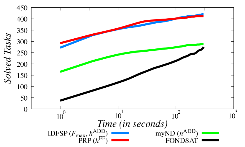
(a) All benchmarks.

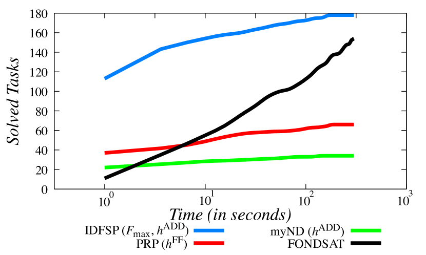
(b) NEW-fond benchmarks.

Figure 4: Solved tasks throughout the range of run-time.

Conclusions

We have developed a novel iterative depth-first search algorithm that efficiently solves fond planning tasks. It considers more explicitly the non-determinism aspect of fond planning, and uses heuristic functions to guide the searching process. We empirically show that our algorithm can outperform existing planners concerning planning time and coverage.

As future work, we intend to investigate how to use the information gathered during previous iterations to make the following iterations of the searching more efficient. We also aim to investigate how to design more informed heuristic functions for fond planning. We aim to study the problem of designing algorithms to extract dual policy solutions, when fairness is not a valid assumption (Camacho and McIlraith 2016; Geffner and Geffner 2018; Rodriguez et al. 2021). We also aim to investigate how to design domains and fond planning tasks that better capture the most significant characteristics of fond planning. These domains and tasks can be used to evaluate new planners.

References

- Bertsekas and Tsitsiklis (1991) Bertsekas, D. P.; and Tsitsiklis, J. N. 1991. An Analysis of Stochastic Shortest Path Problems. Mathematics of Operations Research, 16(3).
- Bonet et al. (2020) Bonet, B.; De Giacomo, G.; Geffner, H.; Patrizi, F.; and Rubin, S. 2020. High-level Programming via Generalized Planning and LTL Synthesis. In KR.
- Bonet and Geffner (2001) Bonet, B.; and Geffner, H. 2001. Planning as Heuristic Search. Artificial Intelligence, 129: 5–33.
- Bonet et al. (2017) Bonet, B.; Giacomo, G. D.; Geffner, H.; and Rubin, S. 2017. Generalized Planning: Non-Deterministic Abstractions and Trajectory Constraints. In IJCAI.
- Brafman and De Giacomo (2019) Brafman, R.; and De Giacomo, G. 2019. Planning for LTLf/LDLf goals in non-markovian fully observable nondeterministic domains. In IJCAI.
- Bryce and Buffet (2008) Bryce, D.; and Buffet, O. 2008. 6th International Planning Competition: Uncertainty Part. International Planning Competition (IPC).
- Camacho et al. (2018) Camacho, A.; Baier, J.; Muise, C.; and McIlraith, S. 2018. Finite LTL Synthesis as Planning. In ICAPS.
- Camacho and McIlraith (2016) Camacho, A.; and McIlraith, S. A. 2016. Strong-Cyclic Planning when Fairness is Not a Valid Assumption. In IJCAI Workshop on Knowledge-Based techniques for Problem Solving.
- Camacho and McIlraith (2019) Camacho, A.; and McIlraith, S. A. 2019. Strong Fully Observable Non-Deterministic Planning with LTL and LTLf Goals. In IJCAI.
- Camacho et al. (2017) Camacho, A.; Triantafillou, E.; Muise, C.; Baier, J.; and McIlraith, S. 2017. Non-Deterministic Planning with Temporally Extended Goals: LTL over Finite and Infinite Traces. In AAAI.
- Cimatti et al. (2003) Cimatti, A.; Pistore, M.; Roveri, M.; and Traverso, P. 2003. Weak, Strong, and Strong Cyclic Planning via Symbolic Model Checking. Artificial Intelligence, 147(1-2).
- De Giacomo and Rubin (2018) De Giacomo, G.; and Rubin, S. 2018. Automata-Theoretic Foundations of FOND Planning for LTLf and LDLf Goals. In IJCAI.
- Fu et al. (2011) Fu, J.; Ng, V.; Bastani, F. B.; and Yen, I. 2011. Simple and Fast Strong Cyclic Planning for Fully-Observable Nondeterministic Planning Problems. In IJCAI.
- Geffner and Geffner (2018) Geffner, T.; and Geffner, H. 2018. Compact Policies for Fully Observable Non-Deterministic Planning as SAT. In ICAPS.
- Hansen and Zilberstein (2001) Hansen, E. A.; and Zilberstein, S. 2001. LAO: A heuristic search algorithm that finds solutions with loops. Artificial Intelligence, 129(1-2): 35–62.
- Hoffmann and Nebel (2001) Hoffmann, J.; and Nebel, B. 2001. The FF Planning System: Fast Plan Generation Through Heuristic Search. Journal of Artificial Intelligence Research, 14: 253–302.
- Hu and Giacomo (2011) Hu, Y.; and Giacomo, G. D. 2011. Generalized Planning: Synthesizing Plans that Work for Multiple Environments. In IJCAI.
- Kissmann and Edelkamp (2009) Kissmann, P.; and Edelkamp, S. 2009. Solving Fully-Observable Non-Deterministic Planning Problems via Translation into a General Game. In KI Advances in AI, volume 5803, 1–8.
- Korf (1985) Korf, R. E. 1985. Depth-First Iterative-Deepening: An Optimal Admissible Tree Search. Artificial Intelligence, 27(1): 97–109.
- Kuter et al. (2008) Kuter, U.; Nau, D. S.; Reisner, E.; and Goldman, R. P. 2008. Using Classical Planners to Solve Nondeterministic Planning Problems. In ICAPS.
- Mattmüller et al. (2010) Mattmüller, R.; Ortlieb, M.; Helmert, M.; and Bercher, P. 2010. Pattern Database Heuristics for Fully Observable Nondeterministic Planning. In ICAPS.
- Mattmüller (2013) Mattmüller, R. 2013. Informed Progression Search for Fully Observable Nondeterministic Planning. Ph.D. thesis, Albert-Ludwigs-Universität Freiburg.
- Muise, Belle, and McIlraith (2014) Muise, C.; Belle, V.; and McIlraith, S. A. 2014. Computing Contingent Plans via Fully Observable Non-Deterministic Planning. In AAAI.
- Muise, McIlraith, and Beck (2012) Muise, C.; McIlraith, S. A.; and Beck, J. C. 2012. Improved Non-deterministic Planning by Exploiting State Relevance. In ICAPS.
- Muise, McIlraith, and Belle (2014) Muise, C.; McIlraith, S. A.; and Belle, V. 2014. Non-Deterministic Planning With Conditional Effects. In ICAPS.
- Patrizi, Lipovetzky, and Geffner (2013) Patrizi, F.; Lipovetzky, N.; and Geffner, H. 2013. Fair LTL Synthesis for Non-Deterministic Systems using Strong Cyclic Planners. In IJCAI.
- Ramírez and Sardiña (2014) Ramírez, M.; and Sardiña, S. 2014. Directed Fixed-Point Regression-Based Planning for Non-Deterministic Domains. In ICAPS.
- Rodriguez et al. (2021) Rodriguez, I. D.; Bonet, B.; Sardiña, S.; and Geffner, H. 2021. Flexible FOND Planning with Explicit Fairness Assumptions. In ICAPS.
- Winterer et al. (2017) Winterer, D.; Alkhazraji, Y.; Katz, M.; and Wehrle, M. 2017. Stubborn Sets for Fully Observable Nondeterministic Planning. In ICAPS.
- Winterer, Wehrle, and Katz (2016) Winterer, D.; Wehrle, M.; and Katz, M. 2016. Structural Symmetries for Fully Observable Nondeterministic Planning. In IJCAI.