Universality of Approximate Message Passing with
Semi-Random Matrices

Abstract

Approximate Message Passing (AMP) is a class of iterative algorithms that have found applications in many problems in high-dimensional statistics and machine learning. In its general form, AMP can be formulated as an iterative procedure driven by a matrix $\boldsymbol{M}$. Theoretical analyses of AMP typically assume strong distributional properties on $\boldsymbol{M}$—for example, $\boldsymbol{M}$ has i.i.d. sub-Gaussian entries or is drawn from a rotational invariant ensemble. However, numerical experiments suggest that the behavior of AMP is universal, as long as the eigenvectors of $\boldsymbol{M}$ are generic. In this paper, we take the first step in rigorously understanding this universality phenomenon. In particular, we investigate a class of “memory-free” AMP algorithms (proposed in Çakmak and Opper [16] for mean-field Ising spin glasses), and show that their asymptotic dynamics is universal on a broad class of “semi-random matrices”. In addition to having the standard rotational invariant ensemble as a special case, the class of semi-random matrices that we define in this work also includes matrices constructed with very limited randomness. One such example is a randomly signed version of the Sine model, introduced in Marinari et al. [47] and Parisi and Potters [60] for spin glasses with fully deterministic couplings.

1 Introduction

Approximate Message Passing (AMP) algorithms are low-complexity iterative algorithms that have attracted considerable attention recently in statistics and machine learning. These algorithms were originally introduced for solving the TAP equations for mean-field spin glasses [13] and in the context of compressed sensing [25]. They are also intricately connected to classical iterative inference algorithms such as belief propagation [49, 40], and expectation propagation [50, 57]. Since their inception, AMP algorithms have found applications in diverse situations—on the one hand, they are directly used as computationally efficient inference algorithms in compressed sensing [25] and coding theory [62]; on the other hand, these algorithms have been used as constructive proof devices to characterize the asymptotic performance of statistical procedures such as the LASSO [5], M-estimators [7, 22, 35, 34], maximum likelihood [67, 66], and spectral methods [54, 52] in high-dimensions.

Given a data matrix $\boldsymbol{M}\in\mathbb{R}^{N\times N}$, an AMP algorithm in its general form consists of the following iterative updates:

$${\boldsymbol{z}}^{(t)} =\boldsymbol{M}F_{t}({\boldsymbol{z}}^{(0)},{\boldsymbol{z}}^{(1)},\dotsc,{\boldsymbol{z}}^{(t-1)})+G_{t}({\boldsymbol{z}}^{(0)},{\boldsymbol{z}}^{(1)},\dotsc,{\boldsymbol{z}}^{(t-1)}).$$ (1)

where $F_{t}\mathrel{\mathop{\ordinarycolon}}\mathbb{R}^{N\times t}\mapsto\mathbb{R}^{N}$ and $G_{t}\mathrel{\mathop{\ordinarycolon}}\mathbb{R}^{N\times t}\mapsto\mathbb{R}^{N}$ are well-chosen vector-valued functions. AMP algorithms are particularly attractive due to their theoretical tractability. Specifically, when the data matrix $\boldsymbol{M}$ is drawn from a rotationally-invariant ensemble (such as the Gaussian orthogonal ensemble), and if the function $G_{t}$ (called the Onsager correction) is suitably chosen based on $F_{t}$, the joint empirical distributions of the iterates ${\boldsymbol{z}}^{(1)},\ldots,{\boldsymbol{z}}^{(t)}$ can be shown to converge to a mean-zero Gaussian process as $N\to\infty$. Moreover, the covariance of this limiting Gaussian process can be explicitly computed via a deterministic recursion known as state evolution [13, 5, 39, 61, 68, 10, 30].

Theoretical analyses of AMP algorithms typically make strong assumptions on the distribution of the matrix $\boldsymbol{M}$—for example, one might assume that the entries of $\boldsymbol{M}$ are i.i.d. Gaussian [13, 5, 39, 10]. Another widely used model assumes that $\boldsymbol{M}$ is rotationally invariant, i.e., its distribution is invariant under conjugation by any deterministic orthogonal matrix [61, 68, 30].

While the idealistic statistical models mentioned above are convenient for mathematical analysis, they do not resemble the data matrices encountered in practice, which are often structured or exhibit strong correlations among the matrix entries. Interestingly, numerical experiments suggest that the behavior of AMP algorithms does not depend too strongly on the precise distribution of the matrix $\boldsymbol{M}$. In fact, it has been observed that [16, 1, 44] the theoretical characterizations obtained under idealistic statistical models remain true for many semi-random (or even deterministic) matrix ensembles. Establishing this universality phenomenon is thus of intrinsic importance, as it allows practitioners to use these theoretical characterizations of AMP with greater confidence in real-life statistical and machine learning applications.

There has been some important recent progress in understanding the universality of AMP algorithms for i.i.d matrices $\boldsymbol{M}$. Specifically, it is now well-understood (see [6, 20]) that the Gaussianity of the entries of $\boldsymbol{M}$ is unnecessary—the distribution of the AMP iterates can be tracked using the same state evolution recursion as long as the entries $\boldsymbol{M}$ are i.i.d. mean-zero, unit-variance sub-Gaussian random variables.

Unfortunately, the existing guarantees do not capture the full-scope of the universality phenomenon observed in practice. A striking example in this regard is the Sine model of Marinari et al. [47] and Parisi and Potters [60], an Ising Model where the coupling matrix is the Discrete Sine Transform Matrix. Using non-rigorous techniques, physicists conjecture that the behavior of this completely deterministic model should be the same as the Random Orthogonal Model (ROM), a fully disordered Ising model whose coupling matrix is given by the rotationally invariant matrix $\boldsymbol{U}\operatorname{diag}(b_{1\mathrel{\mathop{\ordinarycolon}}N})\boldsymbol{U}^{\mkern-1.5mu\mathsf{T}}$, where $\boldsymbol{U}\sim\mathsf{Unif}(\mathbb{O}(N))$ is a Haar matrix and $b_{1\mathrel{\mathop{\ordinarycolon}}N}\overset{\text{\tiny{i.i.d.}}}{\sim}\mathsf{Unif}(\{\pm 1\})$. In the context of AMP algorithms, numerical simulations also suggest the equivalence between the Sine model and the ROM, in that they can be characterized by the same state evolution recursion (see Section 2.3 for supporting numerical evidence). More generally, numerical studies reported in the literature [1, 16] suggest that AMP algorithms exhibit universality properties as long as the eigenvectors of $\boldsymbol{M}$ are generic. Formalizing this conjecture remains squarely beyond existing techniques, and presents a fascinating challenge.

In this paper, we take the first step in understanding this universality phenomenon. In particular, we investigate a sub-class of AMP algorithms that take the form

$${\boldsymbol{z}}^{(t+1)} =\boldsymbol{M}\cdot\left(f_{t+1}({\boldsymbol{z}}^{(t)})-\frac{\langle{f_{t+1}({\boldsymbol{z}}^{(t)})}\;,\;{{\boldsymbol{z}}^{(t)}}\rangle}{\|{\boldsymbol{z}}^{(t)}\|^{2}}\cdot{\boldsymbol{z}}^{(t)}\right).$$ (2)

In the above display, the functions $f_{t}\mathrel{\mathop{\ordinarycolon}}\mathbb{R}\mapsto\mathbb{R}$ and act entry-wise on their arguments. We wish to understand the dynamics of the above algorithm under general assumptions on the matrix $\boldsymbol{M}$, the (coordinate-wise) non-linearities $f_{t}$ and the initialization ${\boldsymbol{z}}^{(0)}$. The algorithm in (2) is a special case of (1). The specific choice of $F_{t}$ made in (1) to obtain (2) ensures that the iterates of the resulting algorithm converge to a Gaussian process as $N\rightarrow\infty$ without any Onsager correction (given by the function $G_{t}$ in (1)). We choose to focus on (2) due to its simple “memory-free” structure, namely, the iterate ${\boldsymbol{z}}^{(t+1)}$ only depends on its immediate predecessor ${\boldsymbol{z}}^{(t)}$. In contrast, the general AMP algorithms in (1) might have to maintain a long memory (that grows with $t$) to ensure that the empirical distributions of ${\boldsymbol{z}}^{(t)}$ are asymptotically Gaussian. The AMP algorithm in (2) was introduced in [16] to approximate the magnetization of Ising spin glasses with orthogonally invariant coupling matrices. Similar memory-free variants of AMP algorithms for rectangular data matrices have been proposed under the names “orthogonal AMP” [43] and “vector approximate message passing” [61, 68].

1.1 Notation

We begin by collecting some notations that will be used throughout this paper.

Some common sets: $\mathbb{N}$ and $\mathbb{R}$ denote the set of positive integers and the set of real numbers respectively. $\mathbb{N}_{0}\overset{\text{\tiny{def}}}{=}\mathbb{N}\cup\{0\}$ is the set of non-negative integers. For each $N\in\mathbb{N}$, $[N]$ denotes the set $\{1,2,3,\dotsc,N\}$ and $\mathbb{O}(N)$ denotes the set of $N\times N$ orthogonal matrices.

Asymptotics: Given a sequence $a_{N}$ and a non-negative sequence $b_{N}$ indexed by $N\in\mathbb{N}$ we say $a_{N}\ll b_{N}$ or $a_{N}=o(b_{N})$ if $a_{N}/b_{N}\rightarrow 0$. Similarly we say $a_{N}\lesssim b_{N}$ or $a_{N}=O(b_{N})$ if there exist fixed constants $\alpha\geq 0$ and $N_{0}\in\mathbb{N}$, such that $|a_{N}|\leq\alpha b_{N}$ for all $N\geq N_{0}$.

Asymptotics for random variables: We use $\overset{\text{\tiny{P}}}{\rightarrow}$ to denote convergence in probability.

Linear Algebra: For a vector $\boldsymbol{v}\in\mathbb{R}^{N}$, $\|\boldsymbol{v}\|_{1},\|\boldsymbol{v}\|,\|\boldsymbol{v}\|_{\infty}$ denote the $\ell_{1}$, $\ell_{2}$ and $\ell_{\infty}$ norms respectively and $\|\boldsymbol{v}\|_{0}$ denotes the number of non-zero coordinates (or sparsity) of $\boldsymbol{v}$. For a matrix $\boldsymbol{A}\in\mathbb{R}^{N\times N}$, we denote the $(i,j)$ entry of $\boldsymbol{A}$ using the corresponding lowercase letter $a_{ij}$. To refer to the $(i,j)$ entry of the matrix product $\boldsymbol{A}\boldsymbol{B}$ we use the notation $(\boldsymbol{A}\boldsymbol{B})_{ij}$. $\|\boldsymbol{A}\|_{\operatorname{op}},\|\boldsymbol{A}\|$ denote the operator (spectral) norm and Frobenius norm of $\boldsymbol{A}$ respectively. On the other hand $\|\boldsymbol{A}\|_{\infty}\overset{\text{\tiny{def}}}{=}\max_{i,j\in[N]}|a_{ij}|$ denotes the entry-wise $\ell_{\infty}$ norm. $\boldsymbol{1}$ denotes the vector $(1,1,\dotsc,1)$, $\boldsymbol{0}$ denotes the vector $(0,0,\dotsc,0)$, and $\boldsymbol{e}_{1},\boldsymbol{e}_{2},\dotsc,\boldsymbol{e}_{N}$ denote the standard basis vectors in $\mathbb{R}^{N}$. $\boldsymbol{I}_{N}$ is the $N\times N$ identity matrix.

Gaussian Distributions and Hermite Polynomials: The univariate Gaussian distribution on $\mathbb{R}$ with mean $\mu$ and variance $\sigma^{2}$ is denoted by $\mathcal{N}\left(\mu,\sigma^{2}\right)$. The multivariate Gaussian distribution on $\mathbb{R}^{N}$ with mean vector $\boldsymbol{\mu}$ and covariance matrix $\boldsymbol{\Sigma}$ is denoted by $\mathcal{N}\left(\boldsymbol{\mu},\boldsymbol{\Sigma}\right)$. For each $i\in\mathbb{N}_{0}$, $H_{i}\mathrel{\mathop{\ordinarycolon}}\mathbb{R}\rightarrow\mathbb{R}$ is denotes the Hermite polynomial of degree $i$. The Hermite polynomials are orthogonal polynomials for the standard Gaussian measure $\mathcal{N}\left(0,1\right)$. This means that for $Z\sim\mathcal{N}\left(0,1\right)$, $\mathbb{E}H_{i}^{2}(Z)=1$ for each $i\in\mathbb{N}_{0}$ and $\mathbb{E}[H_{i}(Z)H_{j}(Z)]=0$ for $i,j\in\mathbb{N}_{0}$ and $i\neq j$ (note that we assume throughout that the Hermite polynomials are normalized to have unit norm under the standard Gaussian measure). The first few Hermite polynomials are $H_{0}(z)=1,\;H_{1}(z)=z,\;H_{2}(z)=(z^{2}-1)/\sqrt{2}$. We refer the reader to O’Donnell [55, Chapter 11] for additional background on Hermite polynomials.

Miscellaneous: For a finite set $A$, $\mathsf{Unif}(A)$ denotes the uniform distribution on $A$. Hence $\mathsf{Unif}(\{\pm 1\})$ and $\mathsf{Unif}(\{\pm 1\}^{N})$ denote the uniform distributions on $\{-1,1\}$ and the $N$-dimensional Boolean hypercube $\{-1,1\}^{N}$, respectively. We use $\mathsf{Unif}(\mathbb{O}(N))$ to denote the Haar measure on the orthogonal group $\mathbb{O}(N)$. For any $i,j\in\mathbb{N}_{0}$, $\delta_{ij}$ denotes the Kronecker delta function, with $\delta_{ij}=1$ if $i=j$ and $\delta_{ij}=0$ otherwise.

1.2 Main Result

Our main result establishes the universality of the AMP algorithm (2) for a wide class of semi-random matrix ensembles $\boldsymbol{M}$, defined below.

Definition 1 (Semi-random Matrix Ensemble).

A semi-random matrix ensemble ${\boldsymbol{M}}^{(N)}\in\mathbb{R}^{N\times N}$ is a sequence of random matrices of the form ${\boldsymbol{M}}^{(N)}={\boldsymbol{S}}^{(N)}{\boldsymbol{\Psi}}^{(N)}{\boldsymbol{S}}^{(N)}$ where,

1. ${\boldsymbol{S}}^{(N)}=\operatorname{diag}(s_{1},s_{2},\dotsc,s_{N})$ with $s_{i}\overset{\text{\tiny{i.i.d.}}}{\sim}\mathsf{Unif}(\{\pm 1\})$.

2. ${\boldsymbol{\Psi}}^{(N)}$ is a sequence of deterministic matrices that satisfy:

   1. $\|{\boldsymbol{\Psi}}^{(N)}\|_{\infty}\lesssim N^{-\frac{1}{2}+\epsilon}$ for all fixed $\epsilon>0$.

   2. $\|{\boldsymbol{\Psi}}^{(N)}\|_{\operatorname{op}}\lesssim 1$.

   3. $\max_{i\neq j}\left|\big{(}{\boldsymbol{\Psi}}^{(N)}{{\boldsymbol{\Psi}}^{(N)}}^{\mkern-1.5mu\mathsf{T}}\big{)}_{ij}\right|\lesssim N^{-\frac{1}{2}+\epsilon}$ for all fixed $\epsilon>0$.

   4. There is a fixed constant $\sigma_{\psi}^{2}\in(0,\infty)$ (independent of $N$) such that,

      $$\max_{i\in[N]}\left|\big{(}{\boldsymbol{\Psi}}^{(N)}{{\boldsymbol{\Psi}}^{(N)}}^{\mkern-1.5mu\mathsf{T}}\big{)}_{ii}-\sigma_{\psi}^{2}\right|\ll 1.$$

If ${\boldsymbol{\Psi}}^{(N)}$ is a sequence of random matrices that satisfy the requirements (2a-2d) on an event with probability $1$:

$$\mathbb{P}\left(\|{\boldsymbol{\Psi}}^{(N)}\|_{\infty}\lesssim N^{-\frac{1}{2}+\epsilon}\;\;\forall\;\epsilon\;>0\right)=1,\;\;\mathbb{P}\left(\max_{i\in[N]}\left|\big{(}{\boldsymbol{\Psi}}^{(N)}{{\boldsymbol{\Psi}}^{(N)}}^{\mkern-1.5mu\mathsf{T}}\big{)}_{ii}-\sigma_{\psi}^{2}\right|\ll 1\right)=1,$$ (3a)

$$\mathbb{P}\left(\max_{i\neq j}\left|\big{(}{\boldsymbol{\Psi}}^{(N)}{{\boldsymbol{\Psi}}^{(N)}}^{\mkern-1.5mu\mathsf{T}}\big{)}_{ij}\right|\lesssim N^{-\frac{1}{2}+\epsilon}\;\;\forall\;\epsilon\;>0\right)=1,\;\;\mathbb{P}\left(\|{\boldsymbol{\Psi}}^{(N)}\|_{\operatorname{op}}\lesssim 1\right)=1,$$ (3b)

we say ${\boldsymbol{M}}^{(N)}$ is a semi-random ensemble with probability $1$.

Remark 1.

The notion of a semi-random matrix ensemble is defined only for a sequence of $N\times N$ matrices of increasing dimension of the form ${\boldsymbol{M}}^{(N)}={\boldsymbol{S}}^{(N)}{\boldsymbol{\Psi}}^{(N)}{\boldsymbol{S}}^{(N)}$. For notational clarity, we will suppress the dependence of $\boldsymbol{M}$ and $\boldsymbol{\Psi}$ on $N$ in our subsequent discussion. This dependence will be assumed implicitly throughout. We will often use the phrase “$\boldsymbol{M}$ is semi-random” as a shorthand for “the sequence of random matrices ${\boldsymbol{M}}^{(N)}$ forms a semi-random matrix ensemble”.

Remark 2.

We call matrix ensembles that satisfy the above definition semi-random because the only randomness in these matrices arises from the random sign diagonal matrix $\boldsymbol{S}$. The conditions (2a)-(2d) on $\boldsymbol{\Psi}$ are fully deterministic. These requirements ensure the entries of $\boldsymbol{\Psi}$ are delocalized, and the rows of $\boldsymbol{\Psi}$ are approximately orthogonal with almost equal norms. In Section 1.3, we show that these assumptions are satisfied for many matrix ensembles.

Remark 3.

The conditions in (3) pertain to tail events and can often be verified using the Borel-Cantelli lemma. See Lemma 2 and its proof in Appendix A.1 for an illustration.

We study the iteration (2) under the following assumption on the initialization.

Assumption 1 (Gaussian Initialization).

The iteration (2) is initalized with ${\boldsymbol{z}}^{(0)}\sim\mathcal{N}\left(\boldsymbol{0},\sigma_{0}^{2}\boldsymbol{I}_{N}\right)$ for some positive constant $\sigma_{0}^{2}>0$ (independent of $N$).

In order to state our main result, we need to introduce the state evolution recursion, which characterizes the dynamics of (2).

State Evolution Recursion.

Fix a $T\in\mathbb{N}_{0}$. Define the state evolution recursion associated with $T$ iterations of (2) as:

$$\sigma_{t+1}^{2} =\sigma_{\psi}^{2}\cdot\mathbb{E}[\widecheck{f}_{t+1}^{2}(Z_{t})]$$ (4a)

$$\rho_{{s,t+1}} =\sigma_{\psi}^{2}\cdot\mathbb{E}[\widecheck{f}_{s}(Z_{s-1})\widecheck{f}_{t+1}(Z_{t})]\;\forall\;s\leq t.$$ (4b)

In the above display:

1. The recursion is initialized with $\sigma_{0}^{2}\mathrel{\mathop{\ordinarycolon}}=\sigma_{0}^{2}$, the parameter from Assumption 1 and $\rho_{0,i}\mathrel{\mathop{\ordinarycolon}}=0$ for each $i\geq 1$.

2. $\sigma_{\psi}^{2}$ is the parameter from Definition 1.

3. For each $t\in\{0,1,\dotsc,T\}$, the vector $(Z_{0},Z_{1},\dotsc,Z_{t})\sim\mathcal{N}\left(\boldsymbol{0},\boldsymbol{\Sigma}_{t}\right)$, where $\boldsymbol{\Sigma}_{t}\in\mathbb{R}^{t+1\times t+1}$ is defined as:

   $$\boldsymbol{\Sigma}_{t} \overset{\text{\tiny{def}}}{=}\begin{bmatrix}\sigma_{0}^{2}&\rho_{0,1}&\rho_{0,2}&\ldots&\rho_{0,t}\\ \rho_{0,1}&\sigma_{1}^{2}&\rho_{1,2}&\ldots&\rho_{1,t}\\ \vdots&\vdots&\vdots&\vdots&\vdots\\ \rho_{0,t}&\rho_{1,t}&\rho_{2,t}&\ldots&\sigma_{t}^{2}\end{bmatrix}.$$ (4c)

4. For each $t\in\{1,2,\dotsc,T\}$, $\widecheck{f}_{t}\mathrel{\mathop{\ordinarycolon}}\mathbb{R}\rightarrow\mathbb{R}$ is given by:

   $$\widecheck{f}_{t}(x)={f}_{t}(x)-\frac{\mathbb{E}[Zf_{t}(\sigma_{t-1}Z)]}{\sigma_{t-1}}\cdot x,\;Z\sim\mathcal{N}\left(0,1\right).$$ (4d)

Remark 4 (Non-degenerate Non-linearities).

Throughout this paper, we will assume that the non-linearities $f_{t}$ are non-degenerate in the sense that $f_{t}$ is not the linear function $x\mapsto\alpha x$ for any $\alpha\in\mathbb{R}$. Since all of our results additionally assume that $f_{1\mathrel{\mathop{\ordinarycolon}}T}$ are continuous functions, this ensures that the variance sequence $\sigma_{1\mathrel{\mathop{\ordinarycolon}}T}^{2}$ is strictly positive. Degenerate non-linearities are not useful for applications since if $f_{t}(x)=\alpha x$ for some $t\in[T]$ an inspection of (2) shows that the corresponding iterate ${\boldsymbol{z}}^{(t)}=\boldsymbol{0}$.

Our results characterize the dynamics of (2) using the following notion of convergence.

Definition 2 (Convergence of Empirical Distributions).

A collection of $k$ random vectors $({\boldsymbol{v}}^{(1)},\dotsc,{\boldsymbol{v}}^{(k)})$ in $\mathbb{R}^{N}$ converges with respect to the Wasserstein-$2$ metric to a random vector $(V_{1},V_{2},\dotsc,V_{k})\in\mathbb{R}^{k}$ in probability as $N\rightarrow\infty$, if for any fixed test function $h\mathrel{\mathop{\ordinarycolon}}\mathbb{R}^{k}\rightarrow\mathbb{R}$ (independent of $N$) that satisfies:

$$|h(\boldsymbol{x})-h(\boldsymbol{y})| \leq L\|\boldsymbol{x}-\boldsymbol{y}\|(1+\|\boldsymbol{x}\|+\|\boldsymbol{y}\|),$$ (5)

for some finite constant $L$, we have,

$$\frac{1}{N}\sum_{i=1}^{N}h({v}^{(1)}_{i},{v}^{(2)}_{i},\dotsc,{v}^{(k)}_{i})\overset{\text{\tiny{P}}}{\rightarrow}\mathbb{E}h(V_{1},V_{2},\dotsc,V_{k}).$$ (6)

We denote convergence in this sense using the notation $({\boldsymbol{v}}^{(1)},{\boldsymbol{v}}^{(2)},\dotsc,{\boldsymbol{v}}^{(k)})\overset{\text{\tiny{$\mathrm{PW}_{2}$}}}{\longrightarrow}(V_{1},V_{2},\dotsc,V_{k})$.

The following is our main result.

Theorem 1.

Fix a non-negative integer $T\in\mathbb{N}_{0}$ and functions $f_{1},f_{2},\dotsc,f_{T}\mathrel{\mathop{\ordinarycolon}}\mathbb{R}\rightarrow\mathbb{R}$. Consider the iteration (2) initialized at ${\boldsymbol{z}}^{(0)}$. Suppose that:

1. ${\boldsymbol{z}}^{(0)}$ satisfies Assumption 1,

2. $\boldsymbol{M}$ is a semi-random matrix ensemble in the sense of Definition 1,

3. The non-linearities $f_{t}$ are continuously differentiable Lipschitz functions.

Then, $({\boldsymbol{z}}^{(0)},{\boldsymbol{z}}^{(1)},\dotsc,{\boldsymbol{z}}^{(T)})\overset{\text{\tiny{$\mathrm{PW}_{2}$}}}{\longrightarrow}(Z_{0},Z_{1},\dotsc,Z_{T})\sim\mathcal{N}\left(\boldsymbol{0},\boldsymbol{\Sigma}_{T}\right)$, where $\boldsymbol{\Sigma}_{T}$ is as defined in (4).

Remark 5.

If $\boldsymbol{M}$ is drawn from a rotationally invariant ensemble, the conclusion of the above theorem follows from the work of Fan [30]. As we show in Lemma 2, rotationally invariant matrices are special cases of the semi-random ensemble in the sense that they satisfy the requirements of Definition 1 with probability $1$. Theorem 1 shows that the state evolution actually holds under significantly weaker assumptions than rotational invariance. Indeed, it has identified a much broader class of matrices $\boldsymbol{M}$ such that the associated AMP algorithm has the same asymptotic dynamics. In this sense, this result can be interpreted as a universality theorem.

Remark 6.

For mean-field Ising models, Çakmak and Opper [16] have proposed algorithms of the form (2) to compute the magnetization vector. In this application, $\boldsymbol{M}$ is a suitably centered resolvent of the coupling matrix for the Ising model. For rotationally invariant coupling matrices (as studied in Çakmak and Opper [16] and Fan and Wu [31]), the resolvent is also rotationally invariant. Hence, the previously mentioned result of Fan [30] can be used to analyze the dynamics of this algorithm. In this context, our results show that the exact rotational invariance of the coupling matrix is unnecessary for the validity of the state evolution. Instead, this characterization is valid as soon as the relevant resolvent matrix is semi-random in the sense of Definition 1. This is indeed valid for many coupling matrices—we provide some examples in Section 2.

In many applications, the non-linearities $f_{t}$ are chosen adaptively so that they have the following convenient property.

Assumption 2 (Divergence-Free Non-Linearities).

The functions $f_{t}\mathrel{\mathop{\ordinarycolon}}\mathbb{R}\rightarrow\mathbb{R}$ satisfy:

$$\mathbb{E}[Zf_{t+1}(\sigma_{t}Z)]=0.$$

A simple choice of non-linearities that satisfy the above divergence-free property are the non-linearities $\widecheck{f}_{t}$ defined in (4d). For divergence-free non-linearities, the iteration (2) can be simplified without changing its dynamics by observing that if the non-linearities have the divergence-free property, the coefficient of the correction term:

$$\frac{\langle{f_{t+1}({\boldsymbol{z}}^{(t)})}\;,\;{{\boldsymbol{z}}^{(t)}}\rangle}{\|{\boldsymbol{z}}^{(t)}\|^{2}}\overset{\text{\tiny{(a)}}}{\approx}\frac{\mathbb{E}[(\sigma_{t}Z)\cdot f_{t+1}(\sigma_{t}Z)]}{\sigma_{t}^{2}}\overset{\text{\tiny{(b)}}}{=}0,$$

where the approximation in (a) follows from Theorem 1 and the equality in (b) follows from the divergence-free property. Hence, we also have the following closely related result.

Theorem 2.

Fix a non-negative integer $T\in\mathbb{N}_{0}$ and functions $f_{1},f_{2},\dotsc,f_{T}\mathrel{\mathop{\ordinarycolon}}\mathbb{R}\rightarrow\mathbb{R}$. Consider the iteration:

$${\boldsymbol{z}}^{(t+1)} =\boldsymbol{M}f_{t+1}({\boldsymbol{z}}^{(t)}),$$ (7)

initialized at ${\boldsymbol{z}}^{(0)}$. Suppose that in addition to all the assumptions of Theorem 1, the non-linearities $f_{t}$ satisfy Assumption 2. Then, $({\boldsymbol{z}}^{(0)},{\boldsymbol{z}}^{(1)},\dotsc,{\boldsymbol{z}}^{(T)})\overset{\text{\tiny{$\mathrm{PW}_{2}$}}}{\longrightarrow}(Z_{0},Z_{1},\dotsc,Z_{T})\sim\mathcal{N}\left(\boldsymbol{0},\boldsymbol{\Sigma}_{T}\right)$, where $\boldsymbol{\Sigma}_{T}$ is as defined in (4).

Remark 7.

Our choice of the random matrix ensemble $\boldsymbol{M}$ is inspired by recent progress in free probability. Specifically, [2] established that delocalized orthogonal matrices with sign and permutation symmetries behave like Haar matrices in the sense that conjugation by these matrices also induces freeness [70, 71]. We emphasize that although our choice is motivated by these results, to the best of our knowledge, the result does not follow from existing results in the free probability literature. Here we design a new approach specifically tailored to the AMP algorithms under consideration.

Remark 8.

Theorem 2 also holds in the situation when the iteration (7) is initialized with the deterministic initialization ${\boldsymbol{z}}^{(0)}=c\boldsymbol{1}$ for any $c\in\mathbb{R}$. To see this, consider an AMP algorithm of the form in (7) with a deterministic initialization:

$${\boldsymbol{z}}^{(0)} =c\boldsymbol{1},\quad{\boldsymbol{z}}^{(t+1)}=\boldsymbol{M}f_{t+1}({\boldsymbol{z}}^{(t)}).$$

Such an algorithm can be implemented using another AMP algorithm of the form in (7) with a random Gaussian initialization to which Theorem 2 applies:

$${\boldsymbol{w}}^{(0)} \sim\mathcal{N}\left(\boldsymbol{0},\boldsymbol{I}_{N}\right),\quad{\boldsymbol{w}}^{(t+1)}=\boldsymbol{M}f_{t+1}({\boldsymbol{w}}^{(t)}).$$

In order to do so, we choose the non-linearity for the first iteration $g_{1}$ as the constant function $g_{1}(w)=f_{1}(c)\;\forall\;w\;\in\;\mathbb{R}$. This choice is divergence-free in the sense of Assumption 2 and ensures that ${\boldsymbol{w}}^{(1)}=f_{1}(c)\cdot\boldsymbol{M}\boldsymbol{1}={\boldsymbol{z}}^{(1)}$. For subsequent iterations, we can take $g_{t}=f_{t}\;\forall\;t\geq 2$, ensuring that ${\boldsymbol{w}}^{(t)}={\boldsymbol{z}}^{(t)}\;\forall\;t\geq 1$.

1.3 Examples of Semi-random Matrix Ensembles

We provide some examples of matrix ensembles which are semi-random in the sense of Definition 1. These examples consist of random matrices that neither have i.i.d. entries nor are rotationally invariant. Consequently, none of the existing results on the state evolution of AMP algorithms apply to these ensembles.

Example 1.

The following lemma shows that any symmetric, delocalized orthogonal matrix conjugated by a random sign diagonal matrix is semi-random in the sense of Definition 1.

Lemma 1.

Let $\boldsymbol{\Psi}\in\mathbb{R}^{N\times N}$ be a symmetric orthogonal matrix with $\|\boldsymbol{\Psi}\|_{\infty}\lesssim N^{-1/2+\epsilon}$ for any $\epsilon>0$. Let $\boldsymbol{S}=\operatorname{diag}(s_{1\mathrel{\mathop{\ordinarycolon}}N})$ be a uniformly random signed diagonal matrix with $s_{1\mathrel{\mathop{\ordinarycolon}}N}\overset{\text{\tiny{i.i.d.}}}{\sim}\mathsf{Unif}(\{\pm 1\})$. Then, $\boldsymbol{M}=\boldsymbol{S}\boldsymbol{\Psi}\boldsymbol{S}$ is semi-random with constant $\sigma_{\psi}^{2}=1$ in the sense of Definition 1.

Proof.

Observe that $\boldsymbol{M}$ satisfies requirement (1) of Definition 1 by construction. Requirement (2a) follows from the delocalization hypothesis. Since $\boldsymbol{\Psi}^{2}=\boldsymbol{I}_{N}$, requirements (2c) and (2d) are also verified. Furthermore, since the spectral measure of symmetric orthogonal matrices is supported on $\{-1,1\}$, $\|\boldsymbol{\Psi}\|_{\operatorname{op}}=1$, which verifies (2b). ∎

Since there are many well-known examples of deterministic, symmetric, delocalized orthogonal matrices (such as the Discrete Cosine Transform matrix, the Discrete Sine Transform matrix, and the Hadamard-Walsh Transform matrices), Lemma 1 shows that our results (Theorem 1 and Theorem 2) apply to matrices constructed with very limited randomness ($N$ random bits). In contrast, prior state evolution results applied exclusively to matrices constructed using $O(N^{2})$ random variables.

Example 2 (Sign and Permutation Invariant Ensembles).

Next, we show that any matrix with delocalized eigenvectors and a “sign and permutation invariance” is also semi-random in the sense of Definition 1.

Lemma 2.

Suppose that $\boldsymbol{M}=\boldsymbol{F}\boldsymbol{\Lambda}\boldsymbol{F}^{\mkern-1.5mu\mathsf{T}}$ where:

1. $\boldsymbol{F}$ is a random orthogonal $N\times N$ matrix which satisfies:

   missingfnum@@desciitemDelocalization:

   $\|\boldsymbol{F}\|_{\infty}\lesssim N^{-1/2+\epsilon}$ for any fixed $\epsilon>0$,

   missingfnum@@desciitemInvariance:

   $\boldsymbol{S}\boldsymbol{F}\boldsymbol{P}\overset{\text{\tiny{d}}}{=}\boldsymbol{F}$ for any signed diagonal matrix $\boldsymbol{S}=\operatorname{diag}{(\boldsymbol{s})},\boldsymbol{s}\in\{\pm 1\}^{N}$ and any $N\times N$ permutation matrix $\boldsymbol{P}$.

2. $\boldsymbol{\Lambda}=\operatorname{diag}(\lambda_{1},\lambda_{2},\dotsc\lambda_{N})$ is a deterministic diagonal matrix such that:

   $$\|\boldsymbol{\Lambda}\|_{\operatorname{op}}\lesssim 1,\quad{\operatorname{Tr}(\boldsymbol{\Lambda})}/{N}\lesssim N^{-1/2+\epsilon}\;\forall\;\epsilon>0,\quad\lim_{N\rightarrow\infty}{\operatorname{Tr}(\boldsymbol{\Lambda}^{2})}/{N}=\sigma_{\psi}^{2}.$$ (8)

Then, there exists a random matrix $\widetilde{\boldsymbol{M}}$, which is semi-random with probability $1$ (cf. Definition 1), and satisfies $\widetilde{\boldsymbol{M}}\overset{\text{\tiny{d}}}{=}{\boldsymbol{M}}$.

We provide the proof of Lemma 2 in Appendix A.1 using a concentration inequality for permutation statistics developed by Bercu et al. [9].

Observe that Lemma 2 implies that the conclusions of Theorem 1 and Theorem 2 also apply to AMP algorithms of the form (2) and (7) driven by a sign and permutation invariant matrix $\boldsymbol{M}$ (cf. Lemma 2). In order to see this, observe that Lemma 2 guarantees the existence of a matrix $\widetilde{\boldsymbol{M}}$ which is semi-random with probability $1$ and satisfies $\boldsymbol{M}\overset{\text{\tiny{d}}}{=}\widetilde{\boldsymbol{M}}$. Let ${\boldsymbol{z}}^{(0)},\dotsc,{\boldsymbol{z}}^{(T)}$ denote the AMP iterates generated by matrix $\boldsymbol{M}$ and ${\widetilde{\boldsymbol{z}}}^{(0)},\dotsc,{\widetilde{\boldsymbol{z}}}^{(T)}$ denote the AMP iterates generated by matrix $\widetilde{\boldsymbol{M}}$. Since $\widetilde{\boldsymbol{M}}$ is semi-random with probability 1 (cf. Lemma 2), by Theorem 1 and Theorem 2, $({\widetilde{\boldsymbol{z}}}^{(0)},\dotsc,{\widetilde{\boldsymbol{z}}}^{(T)})\overset{\text{\tiny{$\mathrm{PW}_{2}$}}}{\longrightarrow}(Z_{0},Z_{1},\dotsc,Z_{T})\sim\mathcal{N}\left(\boldsymbol{0},\boldsymbol{\Sigma}_{T}\right)$, where $\boldsymbol{\Sigma}_{T}$ is as defined in (4). Because $({\boldsymbol{z}}^{(0)},\dotsc,{\boldsymbol{z}}^{(T)})\overset{\text{\tiny{d}}}{=}({\widetilde{\boldsymbol{z}}}^{(0)},\dotsc,{\widetilde{\boldsymbol{z}}}^{(T)})$ (recall $\boldsymbol{M}\overset{\text{\tiny{d}}}{=}\widetilde{\boldsymbol{M}}$), we conclude that $({{\boldsymbol{z}}}^{(0)},\dotsc,{{\boldsymbol{z}}}^{(T)})\overset{\text{\tiny{$\mathrm{PW}_{2}$}}}{\longrightarrow}(Z_{0},Z_{1},\dotsc,Z_{T})\sim\mathcal{N}\left(\boldsymbol{0},\boldsymbol{\Sigma}_{T}\right)$, as claimed.

The sign and permutation invariant model in Lemma 2 is a natural generalization of the rotationally invariant model. This follows as a rotationally invariant matrix is of the form $\boldsymbol{M}=\boldsymbol{U}\boldsymbol{\Lambda}\boldsymbol{U}^{\mkern-1.5mu\mathsf{T}}$ where $\boldsymbol{U}\sim\mathsf{Unif}(\mathbb{O}(N))$ and $\boldsymbol{\Lambda}$ is a deterministic diagonal matrix. Since the Haar measure on $\mathbb{O}(N)$ is invariant to left and right multiplication by arbitrary orthogonal matrices (and in particular sign or permutation matrices), $\boldsymbol{U}\overset{\text{\tiny{d}}}{=}\boldsymbol{S}\boldsymbol{U}\boldsymbol{P}$ for any diagonal sign matrix $\boldsymbol{S}$ and any permutation matrix $\boldsymbol{P}$. Hence, rotationally invariant matrices satisfy the assumptions of Lemma 2. Moreover, given a deterministic diagonal matrix $\boldsymbol{\Lambda}$ satisfying the hypothesis in (8), a delocalized $N\times N$ orthogonal matrix $\boldsymbol{H}$ with $\|\boldsymbol{H}\|_{\infty}\lesssim N^{-1/2+\epsilon}$ for any $\epsilon>0$, a uniformly random $N\times N$ permutation matrix $\boldsymbol{Q}$, and a uniformly random sign diagonal matrix $\boldsymbol{D}$, the matrix

$$\boldsymbol{M}=(\boldsymbol{D}\boldsymbol{H}\boldsymbol{P})\cdot\boldsymbol{\Lambda}\cdot(\boldsymbol{P}^{\mkern-1.5mu\mathsf{T}}\boldsymbol{H}^{\mkern-1.5mu\mathsf{T}}\boldsymbol{D})$$

satisfies the requirements of Lemma 2 by construction. Consequently, sign and permutation invariant matrices can be constructed with significantly less randomness than what is required to construct rotationally invariant matrices.

In many applications, the matrix $\boldsymbol{M}$ used in the AMP algorithm (2) is the resolvent of another random matrix $\boldsymbol{J}$, centered to have zero trace, that is,

$$\boldsymbol{M}(\lambda)=(\lambda\boldsymbol{I}_{N}-\boldsymbol{J})^{-1}-\frac{\operatorname{Tr}((\lambda\boldsymbol{I}_{N}-\boldsymbol{J})^{-1})}{N}\cdot\boldsymbol{I}_{N}.$$ (9)

This is true in the case of the AMP algorithm used by Çakmak and Opper [16] to compute the magnetization of mean-field Ising models with rotationally invariant couplings and for Vector Approximate Message Passing (VAMP) algorithms used in compressed sensing [61, 68]. In these situations, the local law [28] for the random matrix $\boldsymbol{J}$ (if available) can be readily used to verify that $\boldsymbol{M}$ is semi-random (Definition 1). The following two examples show that resolvents of Wigner and sample covariance matrices satisfy the requirements of Definition 1.

Example 3 (Resolvent of Wigner Matrices).

Let $\boldsymbol{J}$ be a Wigner matrix with symmetric entries, that is, $\boldsymbol{J}=\boldsymbol{W}/\sqrt{N}$ for a symmetric matrix $\boldsymbol{W}$ whose entries $W_{ij}$ are i.i.d. symmetric ($W_{ij}\overset{\text{\tiny{d}}}{=}-W_{ij})$ random variables with $\mathbb{E}W_{ij}=0$, $\mathbb{E}W_{ij}^{2}=1+\delta_{ij}$ and finite moments of all orders. These hypotheses are sufficient to guarantee that the spectral measure of $\boldsymbol{J}$ converges to semi-circle distribution supported on $[-2,2]$ [73] and the largest eigenvalue $\lambda_{1}(\boldsymbol{J})\rightarrow 2$ [3]. In this situation, the centered resolvent $\boldsymbol{M}(\lambda)$ in (9) can be shown to satisfy the requirements of Definition 1 for any fixed $\lambda>2$. Indeed, since the entries of $\boldsymbol{W}$ are assumed to be symmetric, requirement (1) of Definition 1 holds. The remaining requirements can be verified using the local law for Wigner matrices. Optimal local laws for Wigner matrices were first obtained by Erdős et al. [29] and we refer the reader to the Erdős and Yau [28, Section 18.2] for additional historical context. In Appendix A.2, we show how the following lemma follows as a consequence of a variant of the local law for Wigner matrices derived by Benaych-Georges and Knowles [8].

Lemma 3.

Let $\boldsymbol{J}$ be a $N\times N$ Wigner matrix with symmetric entries as defined above. For any $\lambda>2$, the matrix $\boldsymbol{M}(\lambda)$ in (9) with this $\boldsymbol{J}$ satisfies the requirements of Definition 1 with constant $\sigma_{\psi}^{2}=-G_{\mathrm{sc}}^{\prime}(\lambda)-G_{\mathrm{sc}}^{2}(\lambda)$ with probability $1-o_{N}(1)$, where $G_{\mathrm{sc}}\mathrel{\mathop{\ordinarycolon}}(2,\infty)\rightarrow\mathbb{R}$ denotes the Cauchy transform of the semi-circle distribution on $[-2,2]$.

Example 4 (Resolvent of Sample Covariance Matrices).

Consider the situation where $\boldsymbol{J}$ is a covariance matrix of the form $\boldsymbol{J}=\boldsymbol{X}^{\mkern-1.5mu\mathsf{T}}\boldsymbol{X}/\sqrt{MN}$ for a $M\times N$ matrix $\boldsymbol{X}$ with a converging aspect ratio $M/N\rightarrow\phi\in(0,\infty)$ whose entries $X_{ij}$ are i.i.d. symmetric ($X_{ij}\overset{\text{\tiny{d}}}{=}-X_{ij}$) random variables with $\mathbb{E}X_{ij}=0$, $\mathbb{E}X_{ij}^{2}=1$ and finite moments of all orders. These hypotheses are sufficient to guarantee that the spectral measure of $\boldsymbol{J}$ converges to the Marchenko-Pastur distribution [46] and $\lambda_{1}(\boldsymbol{J})$, the largest eigenvalue of $\boldsymbol{J}$ satisfies $\lambda_{1}(\boldsymbol{J})\overset{\text{\tiny{P}}}{\rightarrow}\lambda_{+}^{\mathrm{MP}}$ [4] where,

$$\lambda_{+}^{\mathrm{MP}}\overset{\text{\tiny{def}}}{=}\sqrt{\phi}+\frac{1}{\sqrt{\phi}}+2.$$ (10)

For this $\boldsymbol{J}$, we can verify that the centered resolvent matrix $\boldsymbol{M}(\lambda)$ defined in (9) satisfies the requirements of Definition 1 for any $\lambda>\lambda_{+}^{\mathrm{MP}}$. Indeed, since the entries of $\boldsymbol{X}$ are assumed to be symmetric, $\boldsymbol{M}(\lambda)$ satisfies requirement (1) of Definition 1. The remaining requirements can be verified using the local law for sample covariance matrices obtained by Bloemendal et al. [12]. In particular, we have the following result, whose proof appears in Appendix A.3.

Lemma 4.

Let $\boldsymbol{J}$ be a $N\times N$ sample covariance matrix as defined above. For any $\lambda>\lambda_{+}^{\mathrm{MP}}$, the matrix $\boldsymbol{M}(\lambda)$ in (9) with this $\boldsymbol{J}$ satisfies the requirements of Definition 1 with constant $\sigma_{\psi}^{2}=-G_{\mathrm{MP}}^{\prime}(\lambda)-G_{\mathrm{MP}}^{2}(\lambda)$ with probability $1-o_{N}(1)$, where $G_{\mathrm{MP}}\mathrel{\mathop{\ordinarycolon}}(\lambda_{+}^{\mathrm{MP}},\infty)\rightarrow\mathbb{R}$ denotes the Cauchy transform of the Marchenko-Pastur distribution.

2 Applications to Mean-Field Ising Models

As our main application, we discuss how Theorem 2 can be used to obtain a characterization of the dynamics of an iterative algorithm proposed by Çakmak and Opper [16] to compute the magnetization of mean-field Ising spin glass models for several random coupling matrices.

2.1 Background

Mean-Field Ising Spin Glasses.

The mean-field Ising spin glass model is described by the random Gibbs measure on the discrete hypercube $\{\pm 1\}^{N}$:

$$\mu_{N}(\boldsymbol{\sigma}) \overset{\text{\tiny{def}}}{=}Z^{-1}\cdot\exp\left(\frac{\beta}{2}\cdot\boldsymbol{\sigma}^{\mkern-1.5mu\mathsf{T}}\boldsymbol{J}\boldsymbol{\sigma}+\theta\cdot\left\langle{\boldsymbol{1}},{\boldsymbol{\sigma}}\right\rangle\right),$$ (11a)

$$Z \overset{\text{\tiny{def}}}{=}\sum_{\boldsymbol{\sigma}\in\{\pm 1\}^{N}}\exp\left(\frac{\beta}{2}\cdot\boldsymbol{\sigma}^{\mkern-1.5mu\mathsf{T}}\boldsymbol{J}\boldsymbol{\sigma}+\theta\cdot\left\langle{\boldsymbol{1}},{\boldsymbol{\sigma}}\right\rangle\right).$$ (11b)

In the above display, $\boldsymbol{J}$ is a symmetric random coupling matrix and the vector $\boldsymbol{1}=(1,1,\dotsc,1)$ is the external field. The parameter $\beta\geq 0$ is the inverse temperature and the parameter $\theta\geq 0$ regulates the strength of the external field. The thermodynamic properties of this model depend on the spectral measure of the random matrix $\boldsymbol{J}$. Consequently, to study this model in the high-dimensional limit, it is assumed that $\xi_{N}$, the empirical distribution of the eigenvalues $\lambda_{1}(\boldsymbol{J}),\lambda_{2}(\boldsymbol{J}),\dotsc,\lambda_{N}(\boldsymbol{J})$ converges in distribution to a compactly supported, limiting probability measure $\xi$:

$$\xi_{N}\overset{\text{\tiny{def}}}{=}\frac{1}{N}\sum_{i=1}^{N}\delta_{\lambda_{i}(\boldsymbol{J})}\overset{\text{\tiny{d}}}{\rightarrow}\xi.$$ (12a)

Furthermore, this convergence is such that the largest eigenvalue of $$\boldsymbol{J} \xi$$ converges to the rightmost edge of the support of and the smallest eigenvalue remains bounded from below:

$$\max_{i\in[N]}(\lambda_{i}(\boldsymbol{J}))\rightarrow\lambda_{+}\overset{\text{\tiny{def}}}{=}\max\{x\mathrel{\mathop{\ordinarycolon}}x\in\mathrm{Supp}(\xi)\}<\infty,\;\liminf_{N\rightarrow\infty}\min_{i\in[N]}(\lambda_{i}(\boldsymbol{J}))>-\infty.$$ (12b)

Magnetization and the TAP Equations.

A key object of interest for this model is the magnetization, the mean vector of the Gibbs measure:

$$\boldsymbol{\chi}\overset{\text{\tiny{def}}}{=}\sum_{\boldsymbol{\sigma}\in\{\pm 1\}^{N}}\mu_{N}(\boldsymbol{\sigma})\cdot\boldsymbol{\sigma}.$$ (13)

At high temperatures (when $\beta$ is sufficiently small), The magnetization was conjectured to approximately satisfy a system of non-linear fixed point equations, called the Thouless-Anderson-Palmer (TAP) equations, derived by Parisi and Potters [60] and generalized by Opper and Winther [56]:

$$\boldsymbol{\chi} \approx\tanh\Big{(}\theta\cdot\boldsymbol{1}+\beta\cdot\boldsymbol{J}\cdot\boldsymbol{\chi}-\beta\cdot R(\beta-\beta q_{\star})\cdot\boldsymbol{\chi}\Big{)},$$ (14)

where:

1. the function $\tanh(\cdot)$ acts entry-wise on its vector argument.

2. $R(\cdot)$ is the R-transform of the measure $\xi$. This $R$-transform of a probability measure is defined in terms of its Cauchy transform $G\mathrel{\mathop{\ordinarycolon}}[\lambda_{+},\infty)\rightarrow(0,\infty)$:

   $$G(z)\overset{\text{\tiny{def}}}{=}\int\frac{\xi(\mathop{}\!\mathrm{d}\lambda)}{z-\lambda}.$$ (15)

   The Cauchy transform is a strictly decreasing function on $(\lambda_{+},\infty)$ and hence, has a well defined inverse $G^{-1}\mathrel{\mathop{\ordinarycolon}}(0,G(\lambda_{+}))\rightarrow(\lambda_{+},\infty)$. The R-transform is defined on the domain $(0,G(\lambda_{+}))$ and is given by:

   $$R(z)=G^{-1}(z)-1/z.$$ (16)

3. $q_{\star}\in[0,1)$ is the unique solution (guaranteed to exist for small $\beta$ [31, Proposition 1.2]) to the fixed point equation (in q):

   $$q =\mathbb{E}\left[\tanh^{2}\left(\theta+\sigma_{\star}(q)\cdot G\right)\right],\;G\sim\mathcal{N}\left(0,1\right),$$ (17a)

   where,

   $$\sigma^{2}_{\star}(q)\overset{\text{\tiny{def}}}{=}\beta^{2}\cdot{q\cdot R^{\prime}(\beta-\beta q)}.$$ (17b)

This conjecture has been established recently at high-temperature (i.e. for $\beta$ sufficiently small) for rotationally invariant coupling matrices by the third author, in joint work with Yufan Li and Zhou Fan [32].

Solving the TAP equations.

The TAP equations provide a way to compute the magnetization $\boldsymbol{\chi}$ by solving the fixed point equation in (14), which avoids the evaluation of the high-dimensional integral in (13). Çakmak and Opper [16] have proposed the following iterative scheme to compute an approximate solution for the TAP equation (14) at high temperatures (small $\beta$):

$${\boldsymbol{z}}^{(t+1)} =\boldsymbol{M}(\lambda_{\star})\cdot g({\boldsymbol{z}}^{(t)}),$$ (18)

$${\boldsymbol{z}}^{(0)} \sim\mathcal{N}\left(\boldsymbol{0},\sigma^{2}_{\star}(q_{\star})\cdot\boldsymbol{I}_{N}\right).$$ (19)

In the above display,

1. $\boldsymbol{M}(\lambda)$ denotes the resolvent of the interaction matrix $\boldsymbol{J}$ centered to have zero trace:

   $$\boldsymbol{M}(\lambda) =\left(\lambda\cdot\boldsymbol{I}_{N}-\boldsymbol{J}\right)^{-1}-\frac{\operatorname{Tr}[(\lambda\cdot\boldsymbol{I}_{N}-\boldsymbol{J})^{-1}]}{N}\cdot\boldsymbol{I}_{N},$$ (20a)

   and the special value $$\lambda_{\star}$$ is given by:

   $$\lambda_{\star}\overset{\text{\tiny{def}}}{=}G^{-1}(\beta-\beta q_{\star}).$$ (20b)

2. The function $g\mathrel{\mathop{\ordinarycolon}}\mathbb{R}\rightarrow\mathbb{R}$ is defined as:

   $$g(z) =\frac{1}{\beta-\beta q_{\star}}\cdot\left(\frac{\tanh(\theta+z)}{1-q_{\star}}-z\right).$$ (21)

   This function acts entry-wise on its vector arguments in (18).

3. $q_{\star}$ and $\sigma_{\star}^{2}(q_{\star})$ are as defined in (17).

Intuitively, this algorithm can be used to construct a solution to the TAP equations (14) because any fixed point ${\boldsymbol{z}}^{(\infty)}$ of iteration (18) (if it exists) satisfies:

$${\boldsymbol{z}}^{(\infty)}=\boldsymbol{M}(\lambda_{\star})\cdot g({\boldsymbol{z}}^{(\infty)}).$$

Recalling the definitions of $\boldsymbol{M}(\lambda_{\star})$, $g$, the relationship $R(z)=G^{-1}(z)-1/z$ and using the approximation $\xi_{N}\approx\xi$, the above equation can be re-expressed as:

$${\boldsymbol{z}}^{(\infty)}\approx\beta\boldsymbol{J}\tanh(\theta\cdot\boldsymbol{1}+{\boldsymbol{z}}^{(\infty)})-\beta\cdot R(\beta-\beta q_{\star})\cdot\tanh(\theta\cdot\boldsymbol{1}+{\boldsymbol{z}}^{(\infty)}).$$

In particular, ${\boldsymbol{m}}^{(\infty)}\overset{\text{\tiny{def}}}{=}\tanh(\theta\cdot\boldsymbol{1}+{\boldsymbol{z}}^{(\infty)})$ satisfies the TAP equations (14) approximately:

$${\boldsymbol{m}}^{(\infty)} \approx\tanh\Big{(}\theta\cdot\boldsymbol{1}+\beta\cdot\boldsymbol{J}\cdot{\boldsymbol{m}}^{(\infty)}-\beta\cdot R(\beta-\beta q_{\star})\cdot{\boldsymbol{m}}^{(\infty)}\Big{)}.$$

Prior Results.

Çakmak and Opper [16] characterized the asymptotic dynamics of iteration (18) with non-rigorous statistical physics methods. For rotationally invariant coupling matrices $\boldsymbol{J}$, these predictions were rigorously established in Fan and Wu [31]. They used the earlier results of Fan [30], which provides a characterization of a broad class of iterative algorithms involving a rotationally invariant random matrix. The associated state evolution recursion is obtained by instantiating that general state evolution recursion (4) with the following parameters:

1. The parameter $\sigma_{0}^{2}$ which determines the variance of the initialization is set as

   $$\sigma_{0}^{2}\mathrel{\mathop{\ordinarycolon}}=\sigma_{\star}^{2}(q_{\star}),$$ (22a)

   where $\sigma_{\star}^{2}(q_{\star})$ is as defined in (17b).

2. The non-linearities $f_{t}$ are set to

   $$f_{t}=g\quad\forall\;t\;\geq\;1,$$ (22b)

   where the function $g$ is as defined in (21).

3. The parameter $\sigma_{\psi}^{2}$ corresponding to the matrix $\boldsymbol{M}(\lambda_{\star})$ is given by:

   $$\sigma_{\psi}^{2}\overset{\text{\tiny{def}}}{=}\lim_{N\rightarrow\infty}\frac{\operatorname{Tr}(\boldsymbol{M}^{2}(\lambda_{\star}))}{N}\overset{\text{\tiny{(a)}}}{=}\frac{\beta^{2}\cdot(1-q_{\star})^{4}\cdot\sigma_{\star}^{2}(q_{\star})}{q_{\star}-(1-q_{\star})^{2}\sigma_{\star}^{2}(q_{\star})}.$$ (22c)

   In the above display, the equality marked (a) is readily derived by recalling the formula for $\boldsymbol{M}(\lambda_{\star})$ from (20), the definitions of Cauchy and R transforms from (15) and (16) and the formula for $\sigma_{\star}^{2}(q_{\star})$ from (17b).

Because of the special choice of the variance of the initialization in (19), the recursion for $\sigma_{t+1}^{2}$ can be simplified significantly. Indeed, Çakmak and Opper [16, Appendix A1, Equation A7-A8] have shown that the variance $\sigma_{t}^{2}$ remains constant in the recursion:

$$\sigma_{t}^{2}=\sigma_{\star}^{2}(q)\;\forall\;t\;\geq\;0.$$ (23)

The result obtained by Fan [30] and Fan and Wu [31] is quoted below.

Proposition 1 (Fan [30], Fan and Wu [31]).

Suppose the coupling matrix $\boldsymbol{J}=\boldsymbol{U}\boldsymbol{\Lambda}\boldsymbol{U}^{\mkern-1.5mu\mathsf{T}}$ where:

1. $\boldsymbol{U}\sim\mathsf{Unif}(\mathbb{O}(N))$

2. $\boldsymbol{\Lambda}=\operatorname{diag}{(\lambda_{1},\lambda_{2},\dotsc,\lambda_{N})}$ is a deterministic diagonal matrix whose empirical spectral distribution converges to a compactly supported measure $\xi$ in the sense of (12)

Then, for any fixed $T\in\mathbb{N}$, the iteration (18) satisfies $({\boldsymbol{z}}^{(0)},\dotsc,{\boldsymbol{z}}^{(T)})\overset{\text{\tiny{$\mathrm{PW}_{2}$}}}{\longrightarrow}(Z_{0},\dotsc,Z_{T})\sim\mathcal{N}\left(\boldsymbol{0},\boldsymbol{\Sigma}_{T}\right)$ where $\boldsymbol{\Sigma}_{T}$ is the covariance matrix generated by the state evolution recursion (4) with the parameters set as given in (22).

Remark 9.

The result obtained by Fan [30] and Fan and Wu [31] is stronger than the result stated in Proposition 1 in some aspects. For example, these works allow for a general external field (not necessarily the vector $\boldsymbol{1}$). Moreover, they show convergence in a stronger sense than $\mathrm{PW}_{2}$ by obtaining almost sure convergence of empirical averages in (5) (instead of convergence in probability), and by allowing broader classes of test functions which satisfy a weaker analog of the requirement (6).

2.2 Consequences of Theorem 2

As a consequence of Theorem 2, we can show that the characterization of the dynamics of the iteration (18) given in Proposition 1 continues to hold for many matrices beyond the rotationally invariant family. Specifically, we introduce the following four Ising spin glass models.

The Signed Sine Model.

In the signed sine model, the entries of the coupling matrix $\boldsymbol{J}$ are given by:

$$J_{ij}=\frac{2s_{i}s_{j}}{\sqrt{2N+1}}\cdot\sin\left(\frac{2\pi ij}{2N+1}\frac{}{}\right),\;i\in\;[N],\;j\in\;[N].$$ (24)

where $\boldsymbol{s}\sim\mathsf{Unif}(\{\pm 1\}^{N})$ is a uniformly random sign vector. Note that $\boldsymbol{J}=\boldsymbol{S}\boldsymbol{C}\boldsymbol{S}$ where $\boldsymbol{S}=\operatorname{diag}(\boldsymbol{s})$ and $\boldsymbol{C}$ is the Discrete Sine Transform (DST) matrix [15, Section 2.7]. Since the DST matrix $\boldsymbol{C}$ is a symmetric orthogonal matrix, $\boldsymbol{J}^{2}=\boldsymbol{I}_{N}$ (see for e.g. [15, Section 2.8]). As a consequence, the spectrum of $\boldsymbol{J}$ is supported on $\{\pm 1\}$. Furthermore, since $\operatorname{Tr}(\boldsymbol{J})/N\lesssim N^{-1/2}$, the empirical spectral distribution of $\boldsymbol{J}$ converges to $\xi=\mathsf{Unif}(\{\pm 1\})$ in the sense of (12). Our motivation to consider this model comes from the work of Marinari et al. [47] and Parisi and Potters [60] who used statistical physics techniques (high-temperature expansions) and Monte Carlo simulations to demonstrate that many thermodynamic properties of the Ising model with the deterministic coupling matrix $\boldsymbol{C}$ (known as the Sine model) are identical to the corresponding thermodynamic properties of the Ising model where the coupling matrix is $\boldsymbol{U}\boldsymbol{B}\boldsymbol{U}^{\mkern-1.5mu\mathsf{T}}$ where $\boldsymbol{U}\sim\mathsf{Unif}(\mathbb{O}(N))$ is a uniformly random orthogonal matrix and $\boldsymbol{B}=\operatorname{diag}(\boldsymbol{b}),\;\boldsymbol{b}\sim\mathsf{Unif}(\{\pm 1\}^{N})$ is a uniformly random sign diagonal matrix (known as the Random Orthogonal Model). The model in (24) can be thought of as a semi-random analog of the Sine model of Marinari et al. [47]: while it is not fully deterministic, it is significantly less random than the random orthogonal model.

Sign and Permutation Invariant Model.

In the sign and permutation invariant model, the eigenvectors of the coupling matrix $\boldsymbol{J}$ are assumed to be sign and permutation invariant and delocalized. Formally, we assume that $\boldsymbol{J}=\boldsymbol{F}\boldsymbol{\Lambda}\boldsymbol{F}^{\mkern-1.5mu\mathsf{T}}$ where:

1. $\boldsymbol{F}$ is a random orthogonal $N\times N$ matrix which satisfies:

   missingfnum@@desciitemDelocalization:

   $\|\boldsymbol{F}\|_{\infty}\lesssim N^{-1/2+\epsilon}$ for any fixed $\epsilon>0$,

   missingfnum@@desciitemInvariance:

   $\boldsymbol{S}\boldsymbol{F}\boldsymbol{P}\overset{\text{\tiny{d}}}{=}\boldsymbol{F}$ for any signed diagonal matrix $\boldsymbol{S}=\operatorname{diag}{(\boldsymbol{s})},\boldsymbol{s}\in\{\pm 1\}^{N}$ and any $N\times N$ permutation matrix $\boldsymbol{P}$.

2. $\boldsymbol{\Lambda}=\operatorname{diag}(\lambda_{1},\lambda_{2},\dotsc\lambda_{N})$ is a deterministic diagonal matrix whose spectral distribution converges to a compactly supported measure $\xi$ in the sense of (12).

Our motivation to study this model comes from the work of Çakmak and Opper [16] who observed experimentally that such matrices behave like rotationally invariant matrices with regard to the dynamics of the iteration (18).

Sherrington-Kirkpatrick Model.

We also consider the Sherrington-Kirkpatrick (SK) Model [64] where the coupling matrix $\boldsymbol{J}=\boldsymbol{W}/\sqrt{N}$ for a symmetric matrix $\boldsymbol{W}$ whose entries $W_{ij}$ are i.i.d. symmetric ($W_{ij}\overset{\text{\tiny{d}}}{=}-W_{ij})$ random variables with $\mathbb{E}W_{ij}=0$, $\mathbb{E}W_{ij}^{2}=1+\delta_{ij}$ and finite moments of all orders. These hypotheses are sufficient to guarantee that $\xi_{N}$, the spectral measure of $\boldsymbol{J}$ converges to $\xi_{\mathrm{sc}}$, the semicircle distribution supported on $[-2,2]$ in the sense of (12) [73, 3].

Hopfield Model.

Finally, we consider the Hopfield Model [37] where the coupling matrix $\boldsymbol{J}$ is a covariance matrix of the form $\boldsymbol{J}=\boldsymbol{X}^{\mkern-1.5mu\mathsf{T}}\boldsymbol{X}/\sqrt{MN}$ for a $M\times N$ matrix $\boldsymbol{X}$ with a converging aspect ratio $M/N\rightarrow\phi\in(0,\infty)$ whose entries $X_{ij}$ are i.i.d. symmetric ($X_{ij}\overset{\text{\tiny{d}}}{=}-X_{ij}$) random variables with $\mathbb{E}X_{ij}=0$, $\mathbb{E}X_{ij}^{2}=1$ and finite moments of all orders. These hypotheses are sufficient to guarantee that $\xi_{N}$, the spectral measure of $\boldsymbol{J}$ converges to $\xi_{\mathrm{MP}}$, the Marchenko-Pastur distribution in the sense of (12) [46, 4].

Observe that the coupling matrices $\boldsymbol{J}$ corresponding to spin glass models introduced above are not rotationally invariant. Consequently, prior results of Fan [30] and Fan and Wu [31] (quoted in Proposition 1) cannot be used to characterize the dynamics of the iteration (18) for these models. As a corollary of Theorem 2, we obtain the following result, which shows that the asymptotic characterization of the dynamics of (18) given in Proposition 1 continues to hold for these models. This demonstrates a universality phenomenon in the sense that a large class of coupling matrices behave like rotationally invariant coupling matrices with the same limiting spectral distribution as far as the dynamics of (18) is concerned.

Corollary 1.

For any fixed $T\in\mathbb{N}$, the iterations (18) corresponding to:

1. the signed sine model,

2. the sign and permutation invariant model,

3. the Sherrington-Kirkpatrick model, and

4. the Hopfield model

as defined above, satisfy $({\boldsymbol{z}}^{(0)},\dotsc,{\boldsymbol{z}}^{(T)})\overset{\text{\tiny{$\mathrm{PW}_{2}$}}}{\longrightarrow}(Z_{0},\dotsc,Z_{T})\sim\mathcal{N}\left(\boldsymbol{0},\boldsymbol{\Sigma}_{T}\right)$ where $\boldsymbol{\Sigma}_{T}$ is the covariance matrix generated by the state evolution recursion (4) with the parameters set as given in (22).

Proof.

The claim of the corollary is immediate from Theorem 2, once all the assumptions of Theorem 2 have been verified. We begin by observing that the iteration (18) already satisfies many of the properties required by Theorem 2:

1. The matrix $\boldsymbol{M}(\lambda_{\star})$ has bounded operator norm since,

   $$\|\boldsymbol{M}(\lambda_{\star})\|_{\operatorname{op}}\overset{\text{\tiny{\eqref{eq:resolvent}}}}{\leq}\frac{2}{G^{-1}(\beta-\beta q_{\star})-\max_{i\in[N]}(\lambda_{i}(\boldsymbol{J}))}\overset{\text{\tiny{\eqref{eq:support-convergence}}}}{\rightarrow}\frac{2}{G^{-1}(\beta-\beta q_{\star})-\lambda_{+}}<\infty,$$ (25)

   where the final inequality follows from the fact that the inverse Cauchy transform $G^{-1}$ maps its domain $(0,G(\lambda_{+}))$ to the range $(\lambda_{+},\infty)$.

2. The initialization ${\boldsymbol{z}}^{(0)}\sim\mathcal{N}\left(\boldsymbol{0},\sigma_{\star}^{2}(q_{\star})\boldsymbol{I}_{N}\right)$ satisfies Assumption 1.

3. The non-linearity used in the iteration (18) $g(\cdot)$ satisfies is Lipschitz and divergence-free (Assumption 2) since for $Z\sim\mathcal{N}\left(0,1\right)$,

   $$\mathbb{E}[Zg(\sigma_{t}Z)]\overset{\text{\tiny{\eqref{eq:SE-opper-sigma-simple}}}}{=}\mathbb{E}[Zg(\sigma_{\star}Z)] \overset{\text{\tiny{\eqref{eq:g-func}}}}{=}\frac{1}{\beta-\beta q_{\star}}\cdot\left(\frac{\mathbb{E}Z\tanh(\theta+\sigma_{\star}Z)}{1-q_{\star}}-\sigma_{\star}\right)$$

   $$=\frac{\sigma_{\star}}{\beta-\beta q_{\star}}\cdot\left(\frac{1-\mathbb{E}\tanh^{2}(\theta+\sigma_{\star}Z)}{1-q_{\star}}-1\right)\overset{\text{\tiny{\eqref{eq:q-star}}}}{=}0.$$

In order to verify the remaining requirements on $\boldsymbol{M}(\lambda_{\star})$ required by Definition 1, we consider each of the models individually.

Signed Sine Model.

For the signed sine model, since $\boldsymbol{J}^{2}=\boldsymbol{I}_{N}$, the resolvent $(\lambda I_{N}-\boldsymbol{J})^{-1}$ can be expressed as a linear polynomial in $\boldsymbol{J}$. Hence, we have,

$$\boldsymbol{M}(\lambda) \overset{\text{\tiny{def}}}{=}(\lambda\boldsymbol{I}_{N}-\boldsymbol{J})^{-1}-\frac{\operatorname{Tr}[(\lambda\cdot\boldsymbol{I}_{N}-\boldsymbol{J})^{-1}]}{N}\cdot\boldsymbol{I}_{N}=\frac{1}{\lambda^{2}-1}\cdot\left(\boldsymbol{J}-\frac{\operatorname{Tr}(\boldsymbol{J})}{N}\boldsymbol{I}_{N}\right).$$

Recall that for the signed sine model, $\boldsymbol{J}=\boldsymbol{S}\boldsymbol{C}\boldsymbol{S}$ where $\boldsymbol{C}$ is the DST matrix and $\boldsymbol{S}$ is a random sign diagonal matrix. Since the DST matrix is a delocalized and symmetric orthogonal matrix, $\boldsymbol{M}(\lambda)$ is semi-random in the sense of Definition 1 for $\lambda=\lambda_{\star}>1$ by Lemma 1.

Sign and Permutation Invariant Model.

Let $\boldsymbol{J}=\boldsymbol{F}\boldsymbol{\Lambda}\boldsymbol{F}^{\mkern-1.5mu\mathsf{T}}$ denote the eigendecomposition of $\boldsymbol{J}$. Observe that:

$$\boldsymbol{M}(\lambda) \overset{\text{\tiny{def}}}{=}(\lambda\boldsymbol{I}_{N}-\boldsymbol{J})^{-1}-\frac{\operatorname{Tr}[(\lambda\cdot\boldsymbol{I}_{N}-\boldsymbol{J})^{-1}]}{N}\cdot\boldsymbol{I}_{N}=\boldsymbol{F}\cdot\left(\boldsymbol{\Lambda}-\frac{\operatorname{Tr}(\boldsymbol{\Lambda})}{N}\boldsymbol{I}_{N}\right)\cdot\boldsymbol{F}^{\mkern-1.5mu\mathsf{T}}.$$

Hence, $\boldsymbol{M}(\lambda)$ inherits the sign and permutation invariance of $\boldsymbol{J}$. Consequently, $\boldsymbol{M}(\lambda)$ is semi-random in the sense of Definition 1 for $\lambda=\lambda_{\star}>\lambda_{+}$ by Lemma 2.

SK Model.

Here, $\boldsymbol{M}(\lambda)$ satisfies Definition 1 for $\lambda=\lambda_{\star}>2$ by Lemma 3.

Hopfield Model.

Here, $\boldsymbol{M}(\lambda)$ satisfies Definition 1 for $\lambda=\lambda_{\star}>\lambda_{+}^{\mathrm{MP}}$ by Lemma 4.

This concludes the proof of the corollary. ∎

Remark 10.

For the SK model with i.i.d. sub-Gaussian (but not necessarily symmetric) entries, the universality results of Bayati et al. [6] and Chen and Lam [20] can be used to characterize the dynamics of a different iterative algorithm designed by Bolthausen [13] to solve the TAP equation (14). Unlike the iteration in (18), which involves multiplication by the centered resolvent $\boldsymbol{M}(\lambda_{\star})$ at each step, the iteration of Bolthausen [13] involves multiplication by the coupling matrix $\boldsymbol{J}$ at each step.

2.3 Experimental Demonstration of Universality

We end this section with an empirical demonstration of the universality phenomenon studied in Corollary 1. We simulate the dynamics of (18) for three different coupling matrices $\boldsymbol{J}$ of dimension $N=2^{15}$:

missingfnum@@desciitemRandom Orthogonal Ensemble.

Here, we take $\boldsymbol{J}=\boldsymbol{U}\operatorname{diag}(\lambda_{1\mathrel{\mathop{\ordinarycolon}}N})\boldsymbol{U}^{\mkern-1.5mu\mathsf{T}}$ where $\boldsymbol{U}\sim\mathsf{Unif}(\mathbb{O}(N))$ and $\lambda_{1\mathrel{\mathop{\ordinarycolon}}N}\overset{\text{\tiny{i.i.d.}}}{\sim}\mathsf{Unif}(\{\pm 1\})$. Since generating and manipulating Haar matrices of this dimension is prohibitive in terms of memory and run-time, we used the Householder Dice algorithm of the second author [42] to simulate the dynamics of (18) in this case. This algorithm does not require sampling the entire Haar matrix $\boldsymbol{U}$.

missingfnum@@desciitemSigned Hadamard Ensemble.

Here, we take $\boldsymbol{J}=\operatorname{diag}(s_{1\mathrel{\mathop{\ordinarycolon}}N})\boldsymbol{H}\operatorname{diag}(\lambda_{1\mathrel{\mathop{\ordinarycolon}}N})\boldsymbol{H}^{\mkern-1.5mu\mathsf{T}}\operatorname{diag}(s_{1\mathrel{\mathop{\ordinarycolon}}N})$ where $\boldsymbol{H}$ is the $N\times N$ Hadamard-Walsh matrix and $s_{1\mathrel{\mathop{\ordinarycolon}}N},\lambda_{1\mathrel{\mathop{\ordinarycolon}}N}\overset{\text{\tiny{i.i.d.}}}{\sim}\mathsf{Unif}(\{\pm 1\})$. The Hadamard-Walsh matrix is a deterministic orthogonal matrix with entries in $\{-1/\sqrt{N},1/\sqrt{N}\}$.

missingfnum@@desciitemSigned Sine Ensemble.

Here, we take $\boldsymbol{J}=\operatorname{diag}(s_{1\mathrel{\mathop{\ordinarycolon}}N})\boldsymbol{C}\operatorname{diag}(s_{1\mathrel{\mathop{\ordinarycolon}}N})$ where $\boldsymbol{C}$ is the $N\times N$ Discrete Sine Matrix (DST) and $s_{1\mathrel{\mathop{\ordinarycolon}}N}\overset{\text{\tiny{i.i.d.}}}{\sim}\mathsf{Unif}(\{\pm 1\})$. The DST matrix is a deterministic, symmetric orthogonal matrix with entries $C_{ij}=2\sin(2\pi ij/(2N+1))/\sqrt{2N+1}$.

Figure 1 shows the results of this experiment. Observe that each of the above matrices has the property that $\boldsymbol{J}^{2}=\boldsymbol{I}_{N}$. Hence $\xi_{N}$, the spectral distribution of $\boldsymbol{J}$ is supported on the set $\{-1,+1\}$. Furthermore since $\operatorname{Tr}(\boldsymbol{J})/N\overset{\text{\tiny{P}}}{\rightarrow}0$ for each of these matrices, $\xi_{N}\rightarrow\mathsf{Unif}(\{\pm 1\})$ in the sense of (12) for all of the above ensembles. While Proposition 1 only applies to the Random Orthogonal Ensemble, Figure 1 shows that the state evolution accurately describes the dynamics for Signed Hadamard and the Signed Sine ensembles, even though these matrices are significantly less random. Similar empirical observations have been made in previous works [47, 16]. Corollary 1 provides a theoretical explanation for this empirical phenomenon.

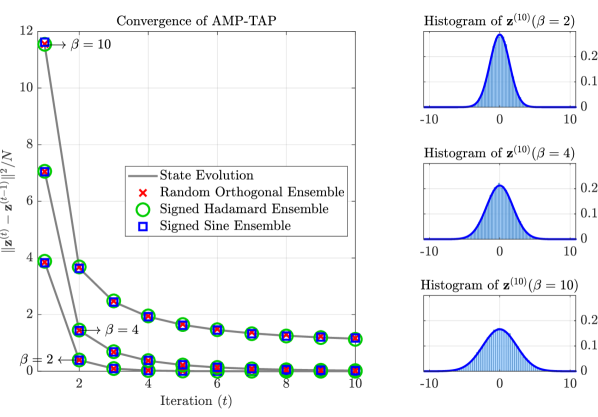
Figure 1: Left: Dynamics of $\|{\boldsymbol{z}}^{(t)}-{\boldsymbol{z}}^{(t-1)}\|^{2}/N$ for the (18) iteration for the Random Orthogonal Ensemble ($\times$), Signed Hadamard Ensemble ($\circ$) and Signed Sine Ensemble ($\square$) compared with predictions from the State Evolution (gray lines) at 3 inverse temperatures $\beta\in\{2,4,10\}$ and external field strength $\theta=2$. Right: Histogram of the empirical distribution of the entries of ${\boldsymbol{z}}^{(10)}$ for the Signed Sine Ensemble compared with the density function of $\mathcal{N}\left(0,\sigma_{10}^{2}\right)$ (dark blue curve) for $\theta=2$ and at 3 inverse temperatures $\beta\in\{2,4,10\}$.

2.4 Ising Models with Deterministic Couplings and Random External Fields

Corollary 1 describes the dynamics of the AMP algorithm of Çakmak and Opper [16] in (18) for Ising models with coupling matrices constructed with very little randomness (such as the signed sine model in (24)). However, it appears to fall short of describing the dynamics of (18) for Ising model with fully deterministic coupling matrices, such as the sine model considered by Marinari et al. [47] and Parisi and Potters [60], where the coupling matrix is given by:

$$J_{ij}=\frac{2}{\sqrt{2N+1}}\cdot\sin\left(\frac{2\pi ij}{2N+1}\frac{}{}\right),\;i\in\;[N],\;j\in\;[N].$$ (26)

For such deterministic coupling matrices, if the external field is not present or is random, Corollary 1 can still be used to analyze the dynamics of the AMP algorithm of Çakmak and Opper [16] via a change-of-variables argument. In order to see this, consider the mean-field Ising spin glass model with the following Gibbs measure on the discrete hypercube $\{\pm 1\}^{N}$:

$$\mu_{N}(\boldsymbol{\sigma}|\boldsymbol{J},\boldsymbol{h}) \overset{\text{\tiny{def}}}{=}\frac{1}{Z(\boldsymbol{J},\boldsymbol{h})}\exp\left(\frac{\beta}{2}\cdot\boldsymbol{\sigma}^{\mkern-1.5mu\mathsf{T}}\boldsymbol{J}\boldsymbol{\sigma}+\theta\cdot\left\langle{\boldsymbol{h}},{\boldsymbol{\sigma}}\right\rangle\right),$$ (27a)

$$Z(\boldsymbol{J},\boldsymbol{h}) \overset{\text{\tiny{def}}}{=}\sum_{\boldsymbol{\sigma}\in\{\pm 1\}^{N}}\exp\left(\frac{\beta}{2}\cdot\boldsymbol{\sigma}^{\mkern-1.5mu\mathsf{T}}\boldsymbol{J}\boldsymbol{\sigma}+\theta\cdot\left\langle{\boldsymbol{h}},{\boldsymbol{\sigma}}\right\rangle\right).$$ (27b)

In the above display, $\boldsymbol{J}$ is a symmetric coupling matrix, the vector $\boldsymbol{h}\in\{\pm 1\}^{N}$ is the external field, the parameter $\beta\geq 0$ is the inverse temperature, and the parameter $\theta\geq 0$ controls the field strength. Observe that the above definitions generalize those in (11), which correspond to the special case where the external field is given by $\boldsymbol{h}=\boldsymbol{1}$. Consider situation when the external field is random:

$$\boldsymbol{h} \sim\mathsf{Unif}(\{\pm 1\}^{N}),$$

but the coupling matrix is deterministic (for instance, the sine model of (26)). In this situation, the AMP algorithm of Çakmak and Opper [16] takes the form:

$${\boldsymbol{z}}^{(t+1)}(\boldsymbol{J},\boldsymbol{h}) =\frac{1}{\beta-\beta q_{\star}}\cdot\boldsymbol{M}(\lambda_{\star})\cdot\left(\frac{\tanh(\theta\boldsymbol{h}+{\boldsymbol{z}}^{(t)}(\boldsymbol{J},\boldsymbol{h}))}{1-q_{\star}}-{\boldsymbol{z}}^{(t)}(\boldsymbol{J},\boldsymbol{h})\right).$$ (28)

In the above display, $q_{\star}$ is as defined in (17) and the matrix $\boldsymbol{M}(\lambda_{\star})$ is the centered resolvent of $\boldsymbol{J}$, as defined in (20). Observe that setting $\boldsymbol{h}=\boldsymbol{1}$ in (28), one obtains the AMP algorithm introduced in (18). Many properties of the Ising model with a deterministic coupling matrix $\boldsymbol{J}$ and a random external field $\boldsymbol{h}$ can be inferred from the corresponding properties of an Ising model with random coupling matrix $\overline{\boldsymbol{J}}\overset{\text{\tiny{def}}}{=}\operatorname{diag}(\boldsymbol{h})\boldsymbol{J}\operatorname{diag}(\boldsymbol{h})$ and a deterministic external field $\boldsymbol{1}$. Indeed, introducing a change of variables $\boldsymbol{\sigma}\leftrightarrow\operatorname{diag}(\boldsymbol{h})\boldsymbol{\sigma}$ in the summation of (27) gives:

$$Z(\boldsymbol{J},\boldsymbol{h}) =Z(\operatorname{diag}(\boldsymbol{h})\cdot\boldsymbol{J}\cdot\operatorname{diag}(\boldsymbol{h}),\boldsymbol{1})=Z(\overline{\boldsymbol{J}},\boldsymbol{1})$$

Similarly, using the fact that $\tanh(\cdot)$ is odd in (28) one obtains:

$${\boldsymbol{z}}^{(t)}(\boldsymbol{J},\boldsymbol{h}) =\operatorname{diag}(\boldsymbol{h})\cdot{\boldsymbol{z}}^{(t)}(\operatorname{diag}(\boldsymbol{h})\boldsymbol{J}\operatorname{diag}(\boldsymbol{h}),\boldsymbol{1})=\operatorname{diag}(\boldsymbol{h})\cdot{\boldsymbol{z}}^{(t)}(\overline{\boldsymbol{J}},\boldsymbol{1}).$$ (29)

In particular, for any even test function $\phi\mathrel{\mathop{\ordinarycolon}}\mathbb{R}^{T+1}\mapsto\mathbb{R}$ which satisfies:

$$\phi(\boldsymbol{z};h) =\phi(-\boldsymbol{z};-h)\quad\forall\;\boldsymbol{z}\in\mathbb{R}^{T},\;h\in\;\mathbb{R},$$ (30)

and

$$|\phi(\boldsymbol{z};h)-\phi(\boldsymbol{z}^{\prime};h)| \leq L\cdot\|\boldsymbol{z}-\boldsymbol{z}^{\prime}\|\cdot(1+\|\boldsymbol{z}\|+\|\boldsymbol{z}^{\prime}\|)\quad\forall\;\boldsymbol{z},\boldsymbol{z}^{\prime}\;\in\;\mathbb{R}^{T},\;h\;\in\;\mathbb{R}$$

for some finite constant $L$, we have:

$$\frac{1}{N}\sum_{i=1}^{N}\phi({z}^{(1)}_{i}(\boldsymbol{J},\boldsymbol{h}),\dotsc,{z}^{(T)}_{i}(\boldsymbol{J},\boldsymbol{h});h_{i}) \overset{\text{\tiny{\eqref{eq:guage-transform}}}}{=}\frac{1}{N}\sum_{i=1}^{N}\phi(h_{i}{z}^{(1)}_{i}(\overline{\boldsymbol{J}},\boldsymbol{1}),\dotsc,h_{i}{z}^{(T)}_{i}(\overline{\boldsymbol{J}},\boldsymbol{1});h_{i})$$ (31)

$$\overset{\text{\tiny{\eqref{eq:test-symmetry}}}}{=}\frac{1}{N}\sum_{i=1}^{N}\phi({z}^{(1)}_{i}(\overline{\boldsymbol{J}},\boldsymbol{1}),\dotsc,{z}^{(T)}_{i}(\overline{\boldsymbol{J}},\boldsymbol{1});1)$$ (32)

$$\overset{\text{\tiny{P}}}{\rightarrow}\mathbb{E}[\phi(Z_{1},\dotsc,Z_{T};1)].$$ (33)

In the above display, the convergence in the last step follows by appealing to Corollary 1. Lastly, we note that many natural quantities of interest can be computed using test functions that satisfy the symmetry requirement in (29). Examples include:

• Taking $\phi(z_{1},\dotsc,z_{T};h)=hz_{t}$ in (31) characterizes the limiting value of the overlap $\left\langle{\boldsymbol{h}},{{\boldsymbol{z}}^{(t)}}\right\rangle/N$ between the AMP iterate ${\boldsymbol{z}}^{(t)}$ and the external field vector $\boldsymbol{h}$.

• Taking $\phi(z_{1},\dotsc,z_{T};h)=(z_{t}-z_{s})^{2}$ in (31) characterizes the limiting value of $\|{\boldsymbol{z}}^{(t)}-{\boldsymbol{z}}^{(s)}\|^{2}/N$, which can be used to detect the convergence/non-convergence of the AMP algorithm in (28).

3 Related Work

Theorem 2 can be thought of as an instance of the following general universality principle.

Properties of a high-dimensional system driven by a generic random matrix $$\boldsymbol{M} \boldsymbol{M}$$ can be accurately predicted by modeling as a rotationally invariant matrix with a matching spectrum. (#)

Indeed, the characterization of the dynamics obtained for (2) in Theorem 1 is precisely the characterization one would “guess” by modeling $\boldsymbol{M}$ as a rotationally invariant matrix and appealing to the results of Fan [30]. Hence, Theorem 1 can be interpreted as a formalization of the universality principle $\eqref{principle}$ in the context of the iterative algorithm (2). Many other instances of this universality principle have been observed and studied, which we will discuss next.

Gaussian Universality.

The simplest instance of the universality principle (# ‣ 3) is observed when the matrix $\boldsymbol{M}$ is a Wigner matrix with i.i.d. entries. In this situation, $\boldsymbol{M}$ often behaves like a Wigner matrix with i.i.d. Gaussian entries, also known as the Gaussian Orthogonal Ensemble. Since this ensemble is rotationally invariant and has the same limiting spectral measure as Wigner matrices (the semi-circle distribution), Gaussian universality can be thought of as a special case of the general universality principle (# ‣ 3). Gaussian universality has been studied from a mathematical perspective in the context of spin-glass models [17, 19], empirical risk minimization in statistical learning [41, 59], and the dynamics of AMP algorithms [6, 20] and general first-order methods [18]. More recently, Gaussian universality has been studied in the case when matrix $\boldsymbol{M}$ has independent rows, with possible correlations within each row. In this situation, $\boldsymbol{M}$ often behaves like a Gaussian matrix with independent rows and matching row covariance. Examples of works that prove Gaussian universality in this situation include the work of Hastie et al. [36] and Mei and Montanari [48] for ridge regression, the work of the second author with Hong Hu [38] for empirical risk minimization with convex loss functions, and the work of Montanari and Saeed [53] for general loss functions.

However, the universality principle (# ‣ 3) appears to extend far beyond examples that can be explained by previously mentioned results on Gaussian universality. Indeed, it has been observed empirically that the universality principle (# ‣ 3) seems to be valid even if the matrix $\boldsymbol{M}$ has very limited randomness. We discuss some of these empirical observations next.

Empirical Observations of Universality.

One instance of the universality principle (# ‣ 3) appears in the context of spin glasses, where Marinari et al. [47] used numerical simulations and high-temperature expansions to demonstrate that many thermodynamic properties of the Sine Model, a mean-field Ising model with a deterministic coupling matrix are nearly identical to the corresponding properties of the Random Orthogonal Model. The coupling matrices of the two models share the same limiting spectral measure. Another instance of the universality principle (# ‣ 3) appears in the field of compressed sensing, where the goal is to reconstruct an unknown sparse signal vector from $n\leq N$ linear measurements of the form, specified using a $n\times N$ sensing matrix $\boldsymbol{A}$. In this context, it has been observed that the performance of many estimators for this problem is nearly identical when $\boldsymbol{A}\mathrel{\mathop{\ordinarycolon}}=\boldsymbol{A}_{\mathrm{PDFT}}$ where $\boldsymbol{A}_{\mathrm{PDFT}}$ denotes the matrix obtained by randomly sub-sampling $n$ rows of $N\times N$ DFT matrix and when $\boldsymbol{A}\mathrel{\mathop{\ordinarycolon}}=\boldsymbol{A}_{\mathrm{Haar}}$ where $\boldsymbol{A}_{\mathrm{Haar}}$ denotes the matrix obtained by sub-sampling $n$ rows of $N\times N$ uniformly random (or Haar distributed) orthogonal matrix. Observations of this type were first reported by Donoho and Tanner [23] and then subsequently in other works [51, 1]. This empirical phenomenon is remarkably robust and is observed even in the presence of measurement noise [58] and for non-linear inference problems beyond compressed sensing like phase retrieval [44, 45]. The performance of many estimators for compressed sensing depends only on the Gram matrix $\boldsymbol{M}=\boldsymbol{A}^{\mkern-1.5mu\mathsf{T}}\boldsymbol{A}$. Since $\boldsymbol{A}_{\mathrm{Haar}}^{\mkern-1.5mu\mathsf{T}}\boldsymbol{A}_{\mathrm{Haar}}$ is a rotationally invariant matrix with the same spectrum as $\boldsymbol{A}_{\mathrm{PDFT}}^{\mkern-1.5mu\mathsf{T}}\boldsymbol{A}_{\mathrm{PDFT}}$, this empirical observation can be viewed as an instance of the universality principle (# ‣ 3).

Though the universality principle (# ‣ 3) has been observed in many different contexts, its mathematical understanding is limited. In what follows we discuss works that study this universality principle from a mathematical viewpoint in specific contexts.

A result from compressed sensing.

In the context of certain linear programming-based estimators for noiseless compressed sensing, Donoho and Tanner [24] provided a proof for the observed universality using results from the theory of random polytopes [72, 21, 74].

Results from free probability.

A different line of work [69, 33, 2] from free probability can also be viewed as a formalization of (# ‣ 3). In this area, a well-known result of Voiculescu [70, 71] shows that given two deterministic matrices $\boldsymbol{A},\boldsymbol{B}$, the matrix $\boldsymbol{A}$ is asymptotically freely independent from the rotationally invariant matrix $\boldsymbol{U}\boldsymbol{B}\boldsymbol{U}^{\mkern-1.5mu\mathsf{T}}$ constructed using a uniformly random orthogonal matrix $\boldsymbol{U}\sim\mathsf{Unif}(\mathbb{O}(N))$. As a consequence, the limiting spectral measure of $\boldsymbol{A}+\boldsymbol{U}\boldsymbol{B}\boldsymbol{U}^{\mkern-1.5mu\mathsf{T}}$ (and more generally of arbitrary matrix polynomials in $\boldsymbol{A},\boldsymbol{U}\boldsymbol{B}\boldsymbol{U}^{\mkern-1.5mu\mathsf{T}}$) can be derived from the limiting spectral measure of $\boldsymbol{A},\boldsymbol{B}$ using an operation called the free additive convolution. Tulino et al. [69] obtained a suprising extension of the results of Voiculescu [70, 71] by showing that in the situation that $\boldsymbol{A},\boldsymbol{B}$ are independent diagonal matrices with i.i.d. diagonal entries, the matrix $\boldsymbol{A}$ is also asymptotically free of the significantly less random matrix $\boldsymbol{F}\boldsymbol{B}\boldsymbol{F}^{\mkern-1.5mu\mathsf{T}}$ where $\boldsymbol{F}$ is the deterministic $N\times N$ Fourier matrix. As a consequence, the limiting spectral distribution $\boldsymbol{A}+\boldsymbol{M}$ is identical in the situation when $\boldsymbol{M}=\boldsymbol{F}\boldsymbol{B}\boldsymbol{F}^{\mkern-1.5mu\mathsf{T}}$ and in the situation when $\boldsymbol{M}=\boldsymbol{U}\boldsymbol{B}\boldsymbol{U}^{\mkern-1.5mu\mathsf{T}}$, a rotationally invariant matrix with the same spectrum as $\boldsymbol{F}\boldsymbol{B}\boldsymbol{F}^{\mkern-1.5mu\mathsf{T}}$. Hence, the result of Tulino et al. [69] can also be viewed as an instance of the universality principle (# ‣ 3). Subsequently, Anderson and Farrell [2] have obtained a far-reaching generalization of the results of Tulino et al. [69] by showing that conjugation by any delocalized orthogonal matrix with certain sign and permutation symmetries is sufficient to induce asymptotic freeness.

Linearized Approximate Message Passing.

In recent joint work with M. Bakhshizadeh [26], the first author formalized this universality principle (# ‣ 3) for the dynamics of linearized AMP algorithms in the context of the phase retrieval problem. Specifically, the authors of [26] establish that the dynamics of linearized AMP algorithms for phase retrieval are identical if the sensing matrix $\boldsymbol{A}\mathrel{\mathop{\ordinarycolon}}=\boldsymbol{A}_{\mathrm{PHWT}}$ or $\boldsymbol{A}\mathrel{\mathop{\ordinarycolon}}=\boldsymbol{A}_{\mathrm{Haar}}$, where $\boldsymbol{A}_{\mathrm{PHWT}}$ denotes the matrix obtained by randomly sub-sampling $n$ columns of $N\times N$ Hadamard-Walsh matrix and when $\boldsymbol{A}_{\mathrm{Haar}}$ denotes the matrix obtained by sub-sampling $n$ columns of $N\times N$ uniformly random (or Haar distributed) orthogonal matrix. Linearized AMP algorithms have the convenient property that ${\boldsymbol{z}}^{(t)}$, which denotes the output of the algorithm at iteration $t$, is a linear transformation of the initialization ${\boldsymbol{z}}^{(0)}$. That is, ${\boldsymbol{z}}^{(t)}=\boldsymbol{R}_{t}{\boldsymbol{z}}^{(0)}$, for a certain random matrix $\boldsymbol{R}_{t}$. Consequently, understanding the dynamics of linearized AMP algorithms boils down to analyzing the trace and certain quadratic forms of the random matrices $\boldsymbol{R}_{t},\boldsymbol{R}_{t}^{2}$. The authors analyze the relevant spectral properties of these matrices by leveraging and extending the proof techniques of the previously discussed work of Tulino et al. [69]. The non-linear AMP algorithms studied in this paper do not have this convenient linear structure, making their analysis more challenging.

4 Proof Outline

It turns out that Theorem 1 and Theorem 2 are equivalent in the sense that any one of them implies the other. Since we will derive Theorem 1 from Theorem 2, we record one side of this equivalence in the following lemma.

Lemma 5.

Theorem 2 implies Theorem 1.

Proof.

See Appendix B. ∎

As a consequence, we focus on providing a road-map to the proof of Theorem 2 in this section. The complete proof is deferred to Section 10.

• We first establish that without loss of generality, we can normalize some of the parameters involved. In particular, we can assume ${\boldsymbol{z}}^{(0)}\sim\mathcal{N}\left(0,\boldsymbol{I}_{N}\right)$, i.e., $\sigma_{0}^{2}=1$. In addition, we can assume that $\boldsymbol{M}$ is semi-random with $\sigma_{\psi}^{2}=1$ (Definition 1) and $\mathbb{E}[f_{t}^{2}(Z)]=1$ for $Z\sim\mathcal{N}(0,1)$ for all $t\geq 1$. We collect these assertions formally in Lemma 17.

• Armed with this normalization, we turn to the main comparison argument in our universality proof: consider any two iteration sequences

  $${\boldsymbol{z}}^{(t+1)}=\boldsymbol{M}f_{t+1}({\boldsymbol{z}}^{(t)}),$$

  $${\boldsymbol{w}}^{(t+1)}=\boldsymbol{Q}f_{t+1}({\boldsymbol{w}}^{(t)}),$$

  started at ${\boldsymbol{z}}^{(0)}={\boldsymbol{w}}^{(0)}\sim\mathcal{N}\left(\boldsymbol{0},\boldsymbol{I}_{N}\right)$. We show that if $\boldsymbol{M}$ and $\boldsymbol{Q}$ both satisfy Definition 1, for suitably “nice” test functions $h\mathrel{\mathop{\ordinarycolon}}\mathbb{R}^{t+1}\to\mathbb{R}$,

  $$\frac{1}{N}\sum_{i=1}^{N}h({z}^{(0)}_{i},{z}^{(1)}_{i},\dotsc,{z}^{(T)}_{i})-\frac{1}{N}\sum_{i=1}^{N}h({w}^{(0)}_{i},{w}^{(1)}_{i},\dotsc,{w}^{(T)}_{i})\overset{\text{\tiny{P}}}{\rightarrow}0.$$ (34)

  Indeed, this establishes that the empirical distribution of the AMP iterates is identical for any matrix ensemble that satisfies Definition 1.

• Finally, we choose $\boldsymbol{Q}=\boldsymbol{U}\boldsymbol{\Lambda}\boldsymbol{U}^{\mkern-1.5mu\mathsf{T}}$, where $\boldsymbol{U}$ is an $N\times N$ Haar matrix, and $\boldsymbol{\Lambda}=\operatorname{diag}(\lambda_{1\mathrel{\mathop{\ordinarycolon}}N})$ is a diagonal matrix with $\lambda_{1\mathrel{\mathop{\ordinarycolon}}N}\overset{\text{\tiny{i.i.d.}}}{\sim}\mathsf{Unif}(\{\pm 1\})$. This ensemble is semi-random in the sense of Definition 1, and is an “integrable” member in this class. In particular, this ensemble is orthogonally invariant, i.e., $\boldsymbol{Q}\stackrel{{\scriptstyle d}}{{=}}\boldsymbol{O}\boldsymbol{Q}\boldsymbol{O}^{\mkern-1.5mu\mathsf{T}}$ for any orthogonal matrix $\boldsymbol{O}$, and the empirical distribution for this iteration can be directly derived from Fan [30] and Fan and Wu [31]. These results show that

  $$\frac{1}{N}\sum_{i=1}^{N}h({w}^{(0)}_{i},{w}^{(1)}_{i},\dotsc,{w}^{(T)}_{i})\overset{\text{\tiny{P}}}{\rightarrow}\mathbb{E}h(Z_{0},Z_{1},\dotsc,Z_{T}),$$ (35)

  where the law of the random vector $(Z_{0},Z_{1},\dotsc Z_{T})$ is as defined in Theorem 2.

Theorem 2 follows upon combining (34) and (35). Our main contribution in this paper is the comparison result (34). We turn to some key ideas underlying its proof. To this end, fix $T\geq 1$. We first approximate the Lipschitz non-linearities $\{f_{t}\mathrel{\mathop{\ordinarycolon}}1\leq t\leq T\}$ and the test function $h$ by an appropriate sequence of polynomials $f_{t}^{(k)}\mathrel{\mathop{\ordinarycolon}}\mathbb{R}\to\mathbb{R}$ and $h^{(k)}\mathrel{\mathop{\ordinarycolon}}\mathbb{R}^{t+1}\to\mathbb{R}$. In addition, the matrix $\boldsymbol{M}$ is perturbed slightly to construct $\hat{\boldsymbol{M}}$ such that $\hat{\boldsymbol{M}}=\boldsymbol{S}\hat{\boldsymbol{\Psi}}\boldsymbol{S}$, and $(\hat{\boldsymbol{\Psi}}\hat{\boldsymbol{\Psi}}^{\mkern-1.5mu\mathsf{T}})_{11}=(\hat{\boldsymbol{\Psi}}\hat{\boldsymbol{\Psi}}^{\mkern-1.5mu\mathsf{T}})_{22}=\dotsb=(\hat{\boldsymbol{\Psi}}\hat{\boldsymbol{\Psi}}^{\mkern-1.5mu\mathsf{T}})_{NN}=1$. The polynomial approximations $\{f_{t}^{(k)}\mathrel{\mathop{\ordinarycolon}}1\leq t\leq T\},h^{(k)}$ and the perturbed matrix $\hat{\boldsymbol{M}}$ are chosen so that the proxy iteration

$${\hat{\boldsymbol{z}}}^{(t+1;k)}=\hat{\boldsymbol{M}}{f}^{(k)}_{t+1}({\hat{\boldsymbol{z}}}^{(t;k)}),$$

initialized at ${\hat{\boldsymbol{z}}}^{(0;k)}={\boldsymbol{z}}^{(0)}$ accurately tracks the output of the original iteration. Formally, we establish that

$$\lim_{k\rightarrow\infty}\limsup_{N\rightarrow\infty}\mathbb{E}\left[\left|\frac{1}{N}\sum_{i=1}^{N}h({z}^{(0)}_{i},{z}^{(1)}_{i},\dotsc,{z}^{(T)}_{i})-\frac{1}{N}\sum_{i=1}^{N}{h}^{(k)}({\hat{z}}^{(0;k)}_{i},{\hat{z}}^{(1;k)}_{i},\dotsc,{\hat{z}}^{(T;k)}_{i})\right|\right] =0.$$ (36)

We establish this approximation in Proposition 6. Note that given (36), to derive the general claim (34), it suffices to establish (34) under the additional assumptions that the non-linearities $\{f_{t}\mathrel{\mathop{\ordinarycolon}}1\leq t\leq T\}$, the test function $h$ are polynomials, and that $(\boldsymbol{\Psi}\boldsymbol{\Psi}^{\mkern-1.5mu\mathsf{T}})_{11}=(\boldsymbol{\Psi}\boldsymbol{\Psi}^{\mkern-1.5mu\mathsf{T}})_{22}=\dotsb=(\boldsymbol{\Psi}\boldsymbol{\Psi}^{\mkern-1.5mu\mathsf{T}})_{NN}=1$. Given these additional assumptions, we first establish that for any matrix $\boldsymbol{M}$ satisfying Definition 1 and $(\boldsymbol{\Psi}\boldsymbol{\Psi}^{\mkern-1.5mu\mathsf{T}})_{11}=(\boldsymbol{\Psi}\boldsymbol{\Psi}^{\mkern-1.5mu\mathsf{T}})_{22}=\dotsb=(\boldsymbol{\Psi}\boldsymbol{\Psi}^{\mkern-1.5mu\mathsf{T}})_{NN}=1$,

$$\mathrm{Var}\left[\frac{1}{N}\sum_{i=1}^{N}h({z}^{(0)}_{i},{z}^{(1)}_{i},\dotsc,{z}^{(T)}_{i})\right]\to 0.$$

The variance bound is derived by an application of the Efron-Stein inequality [14], and is established in Theorem 4. In turn, this implies

$$\frac{1}{N}\sum_{i=1}^{N}h({z}^{(0)}_{i},{z}^{(1)}_{i},\dotsc,{z}^{(T)}_{i})-\mathbb{E}\Big{[}\frac{1}{N}\sum_{i=1}^{N}h({z}^{(0)}_{i},{z}^{(1)}_{i},\dotsc,{z}^{(T)}_{i})\Big{]} \overset{\text{\tiny{P}}}{\rightarrow}0,$$

$$\frac{1}{N}\sum_{i=1}^{N}h({w}^{(0)}_{i},{w}^{(1)}_{i},\dotsc,{w}^{(T)}_{i})-\mathbb{E}\Big{[}\frac{1}{N}\sum_{i=1}^{N}h({w}^{(0)}_{i},{w}^{(1)}_{i},\dotsc,{w}^{(T)}_{i})\Big{]} \overset{\text{\tiny{P}}}{\rightarrow}0.$$

At this point, to complete the proof of (34), it suffices to establish that the limit of the expected empirical average in the display above is equal for any two matrix ensembles $\boldsymbol{M}$ and $\boldsymbol{Q}$ satisfying Definition 1 and $(\boldsymbol{\Psi}\boldsymbol{\Psi}^{\mkern-1.5mu\mathsf{T}})_{11}=(\boldsymbol{\Psi}\boldsymbol{\Psi}^{\mkern-1.5mu\mathsf{T}})_{22}=\dotsb=(\boldsymbol{\Psi}\boldsymbol{\Psi}^{\mkern-1.5mu\mathsf{T}})_{NN}=1$:

$$\lim_{N\rightarrow\infty}\mathbb{E}\left[\frac{1}{N}\sum_{i=1}^{N}h({z}^{(0)}_{i},{z}^{(1)}_{i},\dotsc,{z}^{(T)}_{i})\right] =\lim_{N\rightarrow\infty}\mathbb{E}\left[\frac{1}{N}\sum_{i=1}^{N}h({w}^{(0)}_{i},{w}^{(1)}_{i},\dotsc,{w}^{(T)}_{i})\right].$$ (37)

This is accomplished by the following theorem, which is the main technical contribution of the paper. To formally state this result, we first record the normalization assumption mentioned above for ease of reference in the subsequent discussion.

Assumption 3 (Normalization).

The initialization ${\boldsymbol{z}}^{(0)}$, the matrix ensemble $\boldsymbol{M}=\boldsymbol{S}\boldsymbol{\Psi}\boldsymbol{S}$ and the non-linearities $f_{t}$ satisfy:

1. ${\boldsymbol{z}}^{(0)}\sim\mathcal{N}\left(\boldsymbol{0},\boldsymbol{I}_{N}\right)$ i.e. $\sigma_{0}^{2}=1$.

2. $(\boldsymbol{\Psi}\boldsymbol{\Psi}^{\mkern-1.5mu\mathsf{T}})_{11}=(\boldsymbol{\Psi}\boldsymbol{\Psi}^{\mkern-1.5mu\mathsf{T}})_{22}=\dotsb=(\boldsymbol{\Psi}\boldsymbol{\Psi}^{\mkern-1.5mu\mathsf{T}})_{NN}=1$. In particular, $\sigma_{\psi}^{2}=1$.

3. $\mathbb{E}f^{2}_{t}(Z)=1$ for $Z\sim\mathcal{N}\left(0,1\right)$.

To establish (37) for a general polynomial polynomial $h$, it suffices to prove (37) for any basis for the collection of $(T+1)$-variable polynomials. We will establish (37) for polynomials $h$ that can be expressed as a product of the univariate Hermite polynomials $\{H_{k}\mathrel{\mathop{\ordinarycolon}}k\geq 0\}$ (O’Donnell [55]). The Hermite polynomials form a basis for all univariate polynomials, and thus any $(T+1)$-variable polynomial $h$ can be expressed as a linear combination of these terms. We now present a formal statement.

Theorem 3.

Fix non-negative integers $T\in\mathbb{N}_{0}$, $D\in\mathbb{N}_{0}$ and $k_{0},k_{1},\dotsc,k_{T}\in\mathbb{N}_{0}$ and functions $f_{1},f_{2},\dotsc,f_{T}\mathrel{\mathop{\ordinarycolon}}\mathbb{R}\rightarrow\mathbb{R}$. There is a constant $c$ that depends only on $T,k_{0\mathrel{\mathop{\ordinarycolon}}T},f_{1\mathrel{\mathop{\ordinarycolon}}T}$ such that if,

1. ${\boldsymbol{z}}^{(0)}$ satisfies Assumption 1 and Assumption 3,

2. The matrix ensemble $\boldsymbol{M}=\boldsymbol{S}\boldsymbol{\Psi}\boldsymbol{S}$ is semi-random in the sense of Definition 1 and satisfies Assumption 3,

3. The non-linearities $f_{1\mathrel{\mathop{\ordinarycolon}}T}$ satisfy Assumption 2, Assumption 3 and are polynomials of degree at most $D$,

then, the iterates:

$${\boldsymbol{z}}^{(t+1)}=\boldsymbol{M}f_{t+1}({\boldsymbol{z}}^{(t)}),$$

initialized at ${\boldsymbol{z}}^{(0)}$ satisfy:

$$\lim_{N\rightarrow\infty}\mathbb{E}\left[\frac{1}{N}\sum_{i=1}^{N}H_{k_{0}}({z}^{(0)}_{i})\cdot H_{k_{1}}({z}^{(1)}_{i})\cdot\dotsb\cdot H_{k_{T}}({z}^{(T)}_{i})\right] =c.$$ (38)

Furthermore, for each $t\in[T]$

$$\lim_{N\rightarrow\infty}\mathbb{E}\left[\frac{1}{N}\sum_{i=1}^{N}H_{k_{t}}({z}^{(t)}_{i})\right] =\begin{cases}1&\mathrel{\mathop{\ordinarycolon}}k_{t}=0\\ 0&\mathrel{\mathop{\ordinarycolon}}k_{t}\geq 1\end{cases}.$$ (39)

Note that (37) follows directly from Theorem 3 as the constant $c$ is independent of the matrix ensemble $\mathbf{M}$ (as long as the assumptions of Theorem 3 are satisfied). The reader might naturally wonder why we work with the Hermite polynomials instead of the usual monomials. This choice provides us a simple way to exploit the divergence-free assumption on the non-linearities $f_{1\mathrel{\mathop{\ordinarycolon}}T}$ (Assumption 2). Specifically, for any fixed $t\geq 0$, consider the expansion of the non-linearity $f_{t}$ in the orthonormal basis of Hermite polynomials:

$$f_{t}(z) =\sum_{i=0}^{D}\vartheta_{i}\cdot H_{i}(z),\quad\vartheta_{i}\overset{\text{\tiny{def}}}{=}\mathbb{E}[H_{i}(Z)f_{t}(Z)],\quad Z\sim\mathcal{N}\left(0,1\right).$$

Under the assumptions of Theorem 3, ${\boldsymbol{z}}^{(t)}\overset{\text{\tiny{$\mathrm{PW}_{2}$}}}{\longrightarrow}\mathcal{N}\left(0,1\right)$. Consequently, the divergence-free assumption is equivalent to the condition that the first Hermite coefficient $\vartheta_{1}\overset{\text{\tiny{def}}}{=}\mathbb{E}[Zf_{t}(Z)]$ vanishes, which is easy to exploit in our combinatorial analysis. Another convenient by-product of using the Hermite basis is that it leads to a simple formula for the limit value in (39) and streamlines our analysis. In random matrix theory, Sodin [65] has similarly observed that using orthogonal polynomials for the correct limiting distribution ensures that the resulting combinatorial analysis is better conditioned while implementing the moment method.

4.1 Proof ideas for Theorem 3

We start with a warm-up example to illustrate some of the ideas involved in the general proof. We study the empirical distribution of the single iterate ${\boldsymbol{z}}^{(2)}$ using the test function $h(x)=x$ (the Hermite polynomial of degree $1$). Consider the simple situation where the non-linearities $f_{1}(x)=f_{2}(x)=x^{2}/\sqrt{3}$. Note that $f_{1}$ and $f_{2}$ are divergence free (cf. Assumption 2) since they are even functions. Furthermore, for $Z\sim\mathcal{N}\left(0,1\right)$, $\mathbb{E}[f_{1}^{2}(Z)]=\mathbb{E}[f_{2}^{2}(Z)]=1$. Our goal is to establish that

$$\lim_{N\rightarrow\infty}\mathbb{E}\left[\frac{1}{N}\sum_{i=1}^{N}z_{i}^{(2)}\right] =0.$$ (40)

Step 1: Unrolling.

Our first step is to “unroll” the iterations and express the LHS of (40) as a polynomial in the initialization ${\boldsymbol{z}}^{(0)}$. Specifically, using that ${\boldsymbol{z}}^{(2)}=\boldsymbol{M}f_{2}({\boldsymbol{z}}^{(1)})$, we have

$$\frac{1}{N}\sum_{i=1}^{N}z_{i}^{(2)}=\frac{1}{N}\sum_{i=1}^{N}\sum_{j=1}^{N}m_{ij}\frac{(z_{i}^{(1)})^{2}}{\sqrt{3}}.$$

The RHS of the above display is a polynomial in ${\boldsymbol{z}}^{(1)}$. In order to obtain a polynomial of ${\boldsymbol{z}}^{(0)}$, we further unroll ${\boldsymbol{z}}^{(1)}$ using the fact that ${\boldsymbol{z}}^{(1)}=\boldsymbol{M}f_{1}({\boldsymbol{z}}^{(0)})$:

$$\frac{1}{N}\sum_{i=1}^{N}z_{i}^{(2)} =\frac{1}{\sqrt{3}N}\sum_{i,j=1}^{N}m_{ij}\cdot\left(\sum_{j_{1}=1}^{N}m_{ij_{1}}\frac{(z_{j_{1}}^{(0)})^{2}}{\sqrt{3}}\right)^{2}$$

$$=\frac{1}{3\sqrt{3}N}\sum_{i,j,j_{1},j_{2}=1}^{N}m_{ij}m_{ij_{1}}m_{ij_{2}}(z_{j_{1}}^{(0)})^{2}(z_{j_{2}}^{(0)})^{2}.$$ (41)

Step 2: Computing Expectations.

Next, we compute the expectation of (41) with respect to the randomness in the initialization ${\boldsymbol{z}}^{(0)}\sim\mathcal{N}\left(\boldsymbol{0},\boldsymbol{I}_{N}\right)$ and the random signs $\boldsymbol{S}=\operatorname{diag}(s_{1\mathrel{\mathop{\ordinarycolon}}N})$ used to generate $\boldsymbol{M}=\boldsymbol{S}\boldsymbol{\Psi}\boldsymbol{S}$. Evaluating the expectation with respect to the ${\boldsymbol{z}}^{(0)}$ variables (conditioned on $\boldsymbol{S}$) and using the fact that $\mathbb{E}Z^{4}=3,\mathbb{E}Z^{2}=1$ for $Z\sim\mathcal{N}\left(0,1\right)$, we obtain,

$$\mathbb{E}\left[\frac{1}{N}\sum_{i=1}^{N}z_{i}^{(2)}\Bigg{|}\boldsymbol{S}\right] =\frac{1}{\sqrt{3}N}\sum_{i,j,j_{1}}m_{ij}m_{ij_{1}}^{2}+\frac{1}{3\sqrt{3}N}\sum_{i,j}\sum_{j_{1}\neq j_{2}}m_{ij}m_{ij_{1}}m_{ij_{2}}.$$

$$=\frac{1}{\sqrt{3}N}\sum_{i,j,j_{1}}s_{i}s_{j}\psi_{ij}\psi_{i,j_{1}}^{2}+\frac{1}{3\sqrt{3}N}\sum_{i,j}\sum_{j_{1}\neq j_{2}}s_{i}s_{j}s_{j_{1}}s_{j_{2}}\psi_{ij}\psi_{ij_{1}}\psi_{ij_{2}}.$$

We now evaluate the expectation with respect to the $\boldsymbol{S}$. Starting with the first term, we observe that $\mathbb{E}[s_{i}s_{j}]=0$ unless $i=j$, in which case $\mathbb{E}[s_{i}^{2}]=1$. Similarly, for the second term, $\mathbb{E}[s_{i}s_{j}s_{j_{1}}s_{j_{2}}]=0$ unless $i=j_{1}$, $j=j_{2}$ or $i=j_{2}$, $j=j_{1}$, in which case $\mathbb{E}[s_{j_{1}}^{2}s_{j_{2}}^{2}]=1$. Hence,

$$\mathbb{E}\left[\frac{1}{N}\sum_{i=1}^{N}z_{i}^{(2)}\right] =\frac{1}{\sqrt{3}N}\sum_{i,j}\psi_{ii}\psi_{ij}^{2}+\frac{2}{3\sqrt{3}N}\sum_{i\neq j}\psi_{ii}\psi_{ij}^{2}\overset{\text{\tiny{def}}}{=}\Gamma(\boldsymbol{\Psi}).$$ (42)

Step 3: Combinatorial Estimates.

Observe that at the end of Step 2, we have expressed the empirical first Hermite moment of ${\boldsymbol{z}}^{(2)}$ as a polynomial $\Gamma(\boldsymbol{\Psi})$. In the next step, we leverage combinatorial estimates to argue that for any $\boldsymbol{\Psi}$ that satisfies the assumptions of Theorem 3, $\lim_{N\rightarrow\infty}\Gamma(\boldsymbol{\Psi})$ exists and is universal (that is, identical for any $\boldsymbol{\Psi}$). In the specific case of (42), this step is particularly easy. Indeed by the triangle inequality and the fact that $\|\boldsymbol{\Psi}\|_{\infty}\lesssim N^{-1/2+\epsilon}$, we have

$$\left|\mathbb{E}\left[\frac{1}{N}\sum_{i=1}^{N}z_{i}^{(2)}\right]\right|=\frac{1}{\sqrt{3}N}\sum_{i,j}|\psi_{ii}||\psi_{ij}|^{2}+\frac{2}{3\sqrt{3}N}\sum_{i\neq j}|\psi_{ii}||\psi_{ij}|^{2}\lesssim\frac{1}{N}\cdot N^{2}\cdot N^{-3/2+3\epsilon}=N^{-1/2+3\epsilon},$$ (43)

which converges to zero for $\epsilon>0$ small enough and thus proves (40). The example above illustrates some of the key ideas involved in the proof of Theorem 3. Unfortunately, this simple case does not capture all the intricacies involved in the general proof. In the general case, we can still execute Step 1 and Step 2 to express the empirical mixed Hermite moments of the iterates ${\boldsymbol{z}}^{(0\mathrel{\mathop{\ordinarycolon}}T)}$ (cf. (38)) as a polynomial in $\boldsymbol{\Psi}$. However, the resulting polynomials are more complicated and the crude bound in (43) based on triangle inequality and $\|\boldsymbol{\Psi}\|_{\infty}\lesssim N^{-1/2+\epsilon}$ is no longer adequate (see Fig. 4 for a concrete counterexample). Handling the general case requires the following two additional ideas.

Idea 1: Cancellations.

This idea leverages the property $\|\boldsymbol{\Psi}\boldsymbol{\Psi}^{\mkern-1.5mu\mathsf{T}}-\boldsymbol{I}_{N}\|_{\infty}\lesssim N^{-1/2+\epsilon}$ to improve upon the crude bound in (43). In order to illustrate this technique, consider the polynomial $\Gamma_{1}(\boldsymbol{\Psi})$ defined as:

$$\Gamma_{1}(\boldsymbol{\Psi})\overset{\text{\tiny{def}}}{=}\frac{1}{N}\sum_{i_{1}\neq i_{2}}\sum_{j,k,\ell}\psi_{i_{1}j}\psi_{i_{1}k}\psi_{i_{1}\ell}\psi_{i_{2}j}\psi_{i_{2}k}\psi_{i_{2}\ell}.$$

Observe that the naive estimate based on the triangle inequality and $\|\boldsymbol{\Psi}\|_{\infty}\lesssim N^{-1/2+\epsilon}$ yields:

$$|\Gamma_{1}(\boldsymbol{\Psi})|\overset{\text{\tiny{(a)}}}{\leq}\frac{1}{N}\sum_{i_{1}\neq i_{2}}\sum_{j,k,\ell}|\psi_{i_{1}j}||\psi_{i_{1}k}||\psi_{i_{1}\ell}||\psi_{i_{2}j}||\psi_{i_{2}k}||\psi_{i_{2}\ell}|\lesssim\frac{1}{N}\cdot N^{5}\cdot N^{-3+6\epsilon}=N^{1+6\epsilon}.$$

Thus the above estimate fails to show the existence and universality of $\lim_{N\rightarrow\infty}\Gamma_{1}(\boldsymbol{\Psi})$. The deficiency in the above estimate lies in the use of the triangle inequality in step (a). A better estimate is obtained by leveraging cancellations that arise from the constraint $\|\boldsymbol{\Psi}\boldsymbol{\Psi}^{\mkern-1.5mu\mathsf{T}}-\boldsymbol{I}_{N}\|_{\infty}\lesssim N^{-1/2+\epsilon}$. Indeed we have,

$$|\Gamma_{1}(\boldsymbol{\Psi})| =\frac{1}{N}\left|\sum_{i_{1}\neq i_{2}}\left(\sum_{j=1}^{N}\psi_{i_{1}j}\psi_{i_{2}j}\right)\cdot\left(\sum_{k=1}^{N}\psi_{i_{1}k}\psi_{i_{2}k}\right)\cdot\left(\sum_{\ell=1}^{N}\psi_{i_{1}\ell}\psi_{i_{2}\ell}\right)\right|$$

$$=\frac{1}{N}\left|\sum_{i_{1}\neq i_{2}}(\boldsymbol{\Psi}\boldsymbol{\Psi}^{\mkern-1.5mu\mathsf{T}})_{i_{1},i_{2}}^{3}\right|\leq\frac{1}{N}\sum_{i_{1}\neq i_{2}}|(\boldsymbol{\Psi}\boldsymbol{\Psi}^{\mkern-1.5mu\mathsf{T}})_{i_{1},i_{2}}|^{3}\lesssim\frac{1}{N}\cdot N^{2}\cdot N^{-3/2+3\epsilon}=N^{-1/2+\epsilon},$$

where step (b) follows from $\|\boldsymbol{\Psi}\boldsymbol{\Psi}^{\mkern-1.5mu\mathsf{T}}-\boldsymbol{I}_{N}\|_{\infty}\lesssim N^{-1/2+\epsilon}$. Hence, this estimate shows that $\lim_{N\rightarrow\infty}\Gamma_{1}(\boldsymbol{\Psi})$ exists and is universal for any $\boldsymbol{\Psi}$ that satisfies $\|\boldsymbol{\Psi}\boldsymbol{\Psi}^{\mkern-1.5mu\mathsf{T}}-\boldsymbol{I}_{N}\|_{\infty}\lesssim N^{-1/2+\epsilon}$.

Idea 2: Simplifications.

Here, the idea is that some polynomials can be simplified by leveraging the constraint $(\boldsymbol{\Psi}\boldsymbol{\Psi}^{\mkern-1.5mu\mathsf{T}})_{11}=(\boldsymbol{\Psi}\boldsymbol{\Psi}^{\mkern-1.5mu\mathsf{T}})_{22}=\dotsb=(\boldsymbol{\Psi}\boldsymbol{\Psi}^{\mkern-1.5mu\mathsf{T}})_{NN}=1$. By simplifying the polynomial before applying the cancellation technique described above, one extracts the maximum benefit out of the cancellations described above. This idea can be illustrated using the following polynomial:

$$\Gamma_{2}(\boldsymbol{\Psi})\overset{\text{\tiny{def}}}{=}\frac{1}{N}\sum_{i_{1}\neq i_{2}}\sum_{j,k,\ell}\sum_{m_{1},m_{2},m_{3}}\psi_{i_{1}j}\psi_{i_{1}k}\psi_{i_{1}\ell}\psi_{i_{2}j}\psi_{i_{2}k}\psi_{i_{2}\ell}\psi_{jm_{1}}^{2}\psi_{km_{2}}^{2}\psi_{\ell m_{3}}^{2}.$$

This polynomial can be simplified by evaluating the sum over $m_{1},m_{2},m_{3}$ as follows:

$$\Gamma_{2}(\boldsymbol{\Psi}) \overset{\text{\tiny{}}}{=}\frac{1}{N}\sum_{i_{1}\neq i_{2}}\sum_{j,k,\ell}\psi_{i_{1}j}\psi_{i_{1}k}\psi_{i_{1}\ell}\psi_{i_{2}j}\psi_{i_{2}k}\psi_{i_{2}\ell}\cdot\left(\sum_{m_{1}}\psi_{jm_{1}}^{2}\right)\cdot\left(\sum_{m_{2}}\psi_{km_{2}}^{2}\right)\cdot\left(\sum_{m_{3}}\psi_{\ell m_{3}}^{2}\right)$$

$$=\frac{1}{N}\sum_{i_{1}\neq i_{2}}\sum_{j,k,\ell}\psi_{i_{1}j}\psi_{i_{1}k}\psi_{i_{1}\ell}\psi_{i_{2}j}\psi_{i_{2}k}\psi_{i_{2}\ell}\cdot(\boldsymbol{\Psi}\boldsymbol{\Psi}^{\mkern-1.5mu\mathsf{T}})_{jj}\cdot(\boldsymbol{\Psi}\boldsymbol{\Psi}^{\mkern-1.5mu\mathsf{T}})_{kk}\cdot(\boldsymbol{\Psi}\boldsymbol{\Psi}^{\mkern-1.5mu\mathsf{T}})_{\ell\ell}$$

$$\overset{\text{\tiny{(c)}}}{=}\frac{1}{N}\sum_{i_{1}\neq i_{2}}\sum_{j,k,\ell}\psi_{i_{1}j}\psi_{i_{1}k}\psi_{i_{1}\ell}\psi_{i_{2}j}\psi_{i_{2}k}\psi_{i_{2}\ell}=\Gamma_{1}(\boldsymbol{\Psi}),$$

where step (c) uses the property $(\boldsymbol{\Psi}\boldsymbol{\Psi}^{\mkern-1.5mu\mathsf{T}})_{11}=(\boldsymbol{\Psi}\boldsymbol{\Psi}^{\mkern-1.5mu\mathsf{T}})_{22}=\dotsb=(\boldsymbol{\Psi}\boldsymbol{\Psi}^{\mkern-1.5mu\mathsf{T}})_{NN}=1$. The simplification above reveals that $\Gamma_{2}(\boldsymbol{\Psi})=\Gamma_{1}(\boldsymbol{\Psi})$ and hence $\lim_{N\rightarrow\infty}\Gamma_{2}(\boldsymbol{\Psi})$ also exists and is universal.

4.2 Outline for the remaining paper

In light of the discussion in the previous section, the rest of the paper is organized as follows:

1. Section 5 collects the main technical ingredients required for the proof of Theorem 3, and completes the proof, assuming these intermediate results. Specifically:

   1. Lemma 6 and Lemma 7 expand the mixed Hermite moments in terms of the initialization ${\boldsymbol{z}}^{(0)}$ (Step 1) and evaluate the expectation to identify the terms which have a non-zero contribution in the limit (Step 2). These lemmas are proved in Section 6. Together, these results express the expected mixed Hermite moments of the iterates as a polynomial in the matrix $\boldsymbol{\Psi}$.

   2. Proposition 2 provides an estimate on the magnitude of a class of simple polynomials. This result uses the idea of cancellations described previously (Idea 1) to improve on the naive estimates based on the triangle inequality. We prove Proposition 2 in Section 7.

   3. Before appealing to the improved estimate obtained in Proposition 2, we first simplify the polynomials obtained by the expansion of the mixed moments (Idea 2) in Proposition 3. The proof of this result appears in Section 8.

   4. Proposition 5 leverages the improved estimate of Proposition 2 to show that the behavior of the resulting simplified polynomials is universal. This result is proved in Section 9.

2. Finally, Section 10 explains how the main results of this paper (Theorem 1 and Theorem 2) follow from Theorem 3.

5 Proof of Theorem 3

This section is devoted to the proof of Theorem 3. We begin by introducing the key ingredients involved in the proof of this result. We defer the proof of these intermediate results to later sections.

5.1 Key Results

5.1.1 Unrolling the AMP Iterations.

We begin by expressing the observable of interest:

$$\frac{1}{N}\sum_{i=1}^{N}H_{k_{0}}({z}^{(0)}_{i})\cdot H_{k_{1}}({z}^{(1)}_{i})\cdot\dotsb\cdot H_{k_{T}}({z}^{(T)}_{i})$$ (44)

as a polynomial of the initialization ${\boldsymbol{z}}^{(0)}$. This involves “unrolling” the AMP iterations to express each ${\boldsymbol{z}}^{(t)}$ as a polynomial of ${\boldsymbol{z}}^{(0)}$. The resulting polynomial takes the form of a combinatorial sum over colorings of decorated forests, which we introduce below.

Definition 3 (Decorated Trees and Forests).

A decorated forest $F$ is given by a tuple $(V,E,p,q)$ where:

1. $V=\{1,2,3,\dotsc,|V|\}$ is the set of vertices.

2. $E$ is the set of directed edges.

The sets $(V,E)$ are such that the directed graph given by $(V,E)$ is a directed forest. We define the following notions:

1. If $u\rightarrow v\in E$, we say $u$ is the parent of $v$ and $v$ is a child of $u$. Each vertex in a directed forest has at most one parent.

2. A vertex with no parent is called a root vertex. The set of all root vertices in the forest $F$ is denoted by $\mathscr{R}(F)$. We number the roots as $1,2,\dotsc,$. Hence, $\mathscr{R}(F)=\{1,2,3,\dotsc,|\mathscr{R}(F)|\}$.

3. A root vertex with no children is called a trivial root. The set of all trivial roots in the forest is denoted by $\mathscr{R}_{0}(F)$.

4. For every vertex $u$ we define $c_{u}(F)$ as the number of children of $u$.

5. A non-root vertex with no children is called a leaf. The set of all leaves is denoted by $\mathscr{L}(F)$.

6. A pair of non-root vertices $u,v\in V\backslash\mathscr{R}(F)$ are siblings if they have the same parent.

The forest is decorated with 3 functions

$$0pt{}\mathrel{\mathop{\ordinarycolon}} V\rightarrow\mathbb{N}_{0}=\{0,1,2,3,\dotsc\},$$

$$p\mathrel{\mathop{\ordinarycolon}} V\backslash\mathscr{R}(F)\rightarrow\mathbb{N}=\{1,2,3,\dotsc\},$$

$$q\mathrel{\mathop{\ordinarycolon}} V\rightarrow\mathbb{N}_{0}=\{0,1,2,3,\dotsc\},$$

such that:

1. The height function $0pt{}$ has the following properties:

   1. for any $u\rightarrow v\in E$, $0pt{v}=0pt{u}-1$.

   2. If $0pt{u}=0$, then $u$ has no children $(c_{u}(F)=0)$.

   3. For every vertex $u$ with no children and $q_{u}\geq 1$, we have $0pt{u}=0$.

2. The function $q$ satisfies: for any vertex $u\in V\backslash(\mathscr{L}(F)\cup\mathscr{R}_{0}(F))$, we have,

   $$q_{u}=\sum_{v\in V\mathrel{\mathop{\ordinarycolon}}u\rightarrow v}p_{v}.$$ (45)

If a decorated forest has exactly one root vertex, it is called a decorated tree. See Figure 2 for an example of a small decorated tree.

Figure 2: An example of a decorated forest (Definition 3) with one root (decorated tree).

Next, we introduce the notion of a coloring of a decorated forest.

Definition 4 (Coloring of Decorated Trees and Forests).

A coloring of a decorated forest $F$ with vertex set $V$ is a map $\ell\mathrel{\mathop{\ordinarycolon}}V\rightarrow[N]$. The set of all colorings of a forest $F$ with vertex set $V$ is denoted by $[N]^{V}$.

The colored decorated trees that appear in the polynomial expansion of the observable (44) have additional constraints, which we collect in the definition below.

Definition 5 (Valid Decorated Colorings of Decorated Forests).

A decorated forest $F=(V,E,0pt{},p,q)$ and a coloring $\ell\mathrel{\mathop{\ordinarycolon}}V\rightarrow[N]$ are valid if:

1. For vertices $u,v$ that are siblings in the forest, we have $\ell_{u}\neq\ell_{v}$.

2. $\ell_{u}=\ell_{v}$ for every $u,v\in\mathscr{R}(F)$.

We denote valid decorated colored forests by defining the indicator function $\mathtt{VALID}$ such that $\mathtt{VALID}(F,\ell)=1$ iff $(F,\ell)$ is a valid colored decorated forest and $\mathtt{VALID}(F,\ell)=0$ otherwise. See Figure 3 for an example of a valid coloring of the decorated tree from Figure 2.

Figure 3: An example of a valid coloring (Definition 5) of the decorated tree (Definition 3) from Figure 2.

Armed with these definitions, we can express the observable (44) as a polynomial in the initialization ${\boldsymbol{z}}^{(0)}$.

Lemma 6.

For any $T\in\mathbb{N}_{0}$ and $k_{0},k_{1},\dotsc,k_{T}\in\mathbb{N}_{0}$, we have:

$$\frac{1}{N}\sum_{i=1}^{N}H_{k_{0}}({z}^{(0)}_{i})\cdot H_{k_{1}}({z}^{(1)}_{i})\cdot\dotsb\cdot H_{k_{T}}({z}^{(T)}_{i})=$$

$$\frac{1}{N}\sum_{\begin{subarray}{c}F\in\mathscr{F}_{T}(k_{0},k_{1},\dotsc,k_{T})\\ F=(V,E,0pt{},p,q)\end{subarray}}\sum_{\begin{subarray}{c}\ell\in[N]^{V}\end{subarray}}\alpha(F)\cdot\mathtt{VALID}(F,\ell)\cdot\left(\prod_{u\rightarrow v}m_{\ell_{u}\ell_{v}}^{p_{v}}\right)\cdot\left(\prod_{\begin{subarray}{c}w\in\mathscr{L}(F)\cup\mathscr{R}_{0}(F)\\ q_{w}\geq 1\end{subarray}}H_{q_{w}}({z}^{(0)}_{\ell_{w}})\right).$$ (46a)

In the above display $$\boldsymbol{M}=(m_{ij}) F=(V,E,0pt{},p,q)$$, and for we define the coefficient:

$$\alpha(F) \overset{\text{def}}{=}\left(\prod_{\begin{subarray}{c}u\in V\backslash(\mathscr{L}(F)\cup\mathscr{R}_{0}(F))\end{subarray}}\frac{\sqrt{q_{u}!}}{c_{u}(F)!}\cdot\prod_{v\mathrel{\mathop{\ordinarycolon}}u\rightarrow v}\frac{1}{\sqrt{p_{v}!}}\right)\cdot\left(\prod_{w\in V\backslash\mathscr{R}(F)}\hat{f}_{0pt{w}+1}(p_{w},q_{w})\right),$$ (46b)

$$\hat{f}_{t}(p,q) \overset{\text{\tiny{def}}}{=}\mathbb{E}[H_{p}\circ f_{t}(Z)\cdot H_{q}(Z)],\;Z\sim\mathcal{N}\left(0,1\right).$$ (46c)

Furthermore, $$\mathscr{F}_{T}(k_{0},k_{1},\dotsc,k_{T}) T+1 \mathscr{R}(F)=\{1,2,\dotsc,T+1\} 0pt{1}=0,0pt{2}=1,\dotsc 0pt{T+1}=T q_{1}=k_{0},q_{2}=k_{1},\dotsc,q_{T+1}=k_{T}$$ denotes the set of all decorated forests with roots, and and .

We defer the proof of Lemma 6 to Section 6.1.

5.1.2 Partitions on a Decorated Tree

Our next step is to evaluate the expectation of the formula (46a) with respect to the randomness in the initialization ${\boldsymbol{z}}^{(0)}\sim\mathcal{N}\left(\boldsymbol{0},\boldsymbol{I}_{N}\right)$ and the uniformly random signed diagonal matrix $\boldsymbol{S}$ used to generate the matrix $\boldsymbol{M}=\boldsymbol{S}\boldsymbol{\Psi}\boldsymbol{S}$. Observe that in order to evaluate the expectation of the RHS of (46a), the repetition pattern of the coloring $\ell\in[N]^{V}$ is important—for two vertices $u,v$ that have the same color $\ell_{u}=\ell_{v}$, the corresponding Gaussian and sign variables are identical ${z}^{(0)}_{\ell_{u}}={z}^{(0)}_{\ell_{v}},s_{\ell_{u}}=s_{\ell_{v}}$. On the other hand, for vertices $u,v$ with different colors $\ell_{u}\neq\ell_{v}$, the corresponding Gaussian and sign variables are independent. The repetition pattern of a coloring in $\ell\in[N]^{V}$ can be encoded by a partition of the vertex set $V$. This motivates the following definitions.

Definition 6 (Partitions and Configurations).

Given a decorated forest $F=(V,E,0pt{},p,q)$, a partition $\pi$ of the vertex set $V$ is a collection of disjoint subsets (called blocks) $\{B_{1},B_{2},\dotsc,B_{s}\}$ such that

$$\bigcup_{j=1}^{s}B_{j}=V,\;B_{j}\cap B_{k}=\emptyset\;\forall\;j\neq k.$$

We define $|\pi|$ to be the number of blocks in $\pi$. For every $v\in V$, we use $\pi(v)$ to denote the unique block $j\in[|\pi|]$ such that $v\in B_{j}$. The set of all partitions of $V$ is denoted by $\mathscr{P}(V)$. A configuration is a pair $(F,\pi)$ consisting of a decorated forest $F$ and a partition $\pi$ of its vertices.

Definition 7 (Colorings consistent with a partition).

Let $\pi$ be a partition of the vertex set $V$ of a decorated forest $F=(V,E,0pt{},p,q)$. A coloring consistent with $\pi$ is a function $\ell\mathrel{\mathop{\ordinarycolon}}V\rightarrow[N]$ such that,

$$\ell_{u}=\ell_{v} \Leftrightarrow\pi(u)=\pi(v).$$

The set of all colorings that are consistent with a partition $\pi$ is denoted by $\mathscr{C}(\pi)$.

Note that whether a pair $(F,\ell)$ is valid colored forest or not depends only on the $(F,\pi)$ where $\pi$ is a partition corresponding to $\ell$. Hence we introduce the following definition.

Definition 8 (Valid Configurations).

A decorated forest $F=(V,E,0pt{},p,q)$ and a partition $\pi\in\mathscr{P}(V)$ form a valid configuration if:

1. For vertices $u,v$ that are siblings in the forest, we have $\pi(u)\neq\pi(v)$.

2. For every $u,v\in\mathscr{R}(F)$, $\pi(u)=\pi(v)$.

We denote valid configurations by defining the indicator function $\mathtt{VALID}$ such that $\mathtt{VALID}(F,\pi)=1$ iff $(F,\pi)$ is a valid configuration and $\mathtt{VALID}(F,\pi)=0$ otherwise.

Observe that as a consequence of the above definitions, (46a) can be rearranged to the following form:

$$\frac{1}{N}\sum_{\ell=1}^{N}H_{k_{0}}({z}^{(0)}_{i})\cdot H_{k_{1}}({z}^{(1)}_{i})\cdot\dotsb\cdot H_{k_{T}}({z}^{(T)}_{i})=$$

$$\frac{1}{N}\sum_{\begin{subarray}{c}F\in\mathscr{F}_{T}(k_{0},k_{1},\dotsc,k_{T})\\ F=(V,E,0pt{},p,q)\end{subarray}}\sum_{\pi\in\mathscr{P}(V)}\sum_{\begin{subarray}{c}\ell\in\mathscr{C}(\pi)\end{subarray}}\alpha(F)\cdot\mathtt{VALID}(F,\pi)\cdot\left(\prod_{u\rightarrow v}m_{\ell_{u}\ell_{v}}^{p_{v}}\right)\cdot\left(\prod_{\begin{subarray}{c}w\in\mathscr{L}(F)\cup\mathscr{R}_{0}(F)\\ q_{w}\geq 1\end{subarray}}H_{q_{w}}({z}^{(0)}_{\ell_{w}})\right).$$ (47)

5.1.3 The Expectation Formula

The expansion in (5.1.2) facilitates the evaluation of the expectation of the polynomial expansion (46a) obtained in Lemma 6. The following lemma identifies the expected value, and identifies the configurations $(F,\pi)$ which have a non-zero contribution to the expectation.

Lemma 7 (The Expectation Formula).

For any $T\in\mathbb{N}_{0}$ and any $k_{0},k_{2},k_{3},\dotsc,k_{T}\in\mathbb{N}_{0}$, we have,

$$\mathbb{E}\left[\frac{1}{N}\sum_{\ell=1}^{N}H_{k_{0}}({z}^{(0)}_{i})\cdot H_{k_{1}}({z}^{(1)}_{i})\cdot\dotsb\cdot H_{k_{T}}({z}^{(T)}_{i})\right]=$$

$$\hskip 56.9055pt\sum_{\begin{subarray}{c}F\in\mathscr{F}_{T}(k_{0},k_{1},\dotsc,k_{T})\\ F=(V,E,0pt{},p,q)\end{subarray}}\sum_{\pi\in\mathscr{P}(V)}\sum_{\begin{subarray}{c}\ell\in\mathscr{C}(\pi)\end{subarray}}\alpha(F)\cdot\mathtt{VALID}(F,\pi)\cdot\beta_{1}(F,\pi)\cdot\beta_{2}(F,\pi)\cdot\gamma(\boldsymbol{\Psi};F,\ell).$$ (48a)

For a decorated forest $$F=(V,E,0pt{},p,q) \pi=\{B_{1},B_{2},\dotsc,B_{\pi}\} \alpha(F)$$ and a partition recall from (46c). Further, we define:

$$\beta_{1}(F,\pi) \overset{\text{\tiny{def}}}{=}\prod_{j=1}^{|\pi|}\mathbb{E}\left[\prod_{\begin{subarray}{c}v\in(\mathscr{L}(F)\cup\mathscr{R}_{0}(F))\cap B_{j}\\ q_{v}\geq 1\end{subarray}}H_{q_{v}}(Z)\right],$$ (48b)

$$\beta_{2}(F,\pi) \overset{\text{\tiny{def}}}{=}\prod_{j=1}^{|\pi|}\mathbb{E}\left[\left(\prod_{u\in(B_{j}\cap\mathscr{R}(F))\backslash\mathscr{R}_{0}(F)}S^{q_{u}}\right)\cdot\left(\prod_{v\in B_{j}\cap\mathscr{L}(F)}S^{p_{v}}\right)\cdot\left(\prod_{\begin{subarray}{c}u\in B_{j}\backslash(\mathscr{L}(F)\cup\mathscr{R}(F))\end{subarray}}S^{p_{u}+q_{u}}\right)\right],$$ (48c)

$$\gamma(\boldsymbol{\Psi};F,\ell) \overset{\text{\tiny{def}}}{=}\frac{1}{N}\prod_{\begin{subarray}{c}e\in E\\ e=u\rightarrow v\end{subarray}}\psi_{\ell_{u}\ell_{v}}^{p_{v}},$$ (48d)

where $$Z\sim\mathcal{N}\left(0,1\right) S\sim\mathsf{Unif}(\{\pm 1\}) \alpha(F)\cdot\mathtt{VALID}(F,\pi)\cdot\beta_{1}(F,\pi)\cdot\beta_{2}(F,\pi)=0 (F,\pi)$$ and . Furthermore, , unless form a relevant configuration, defined below.

Definition 9 (Relevant Configuration).

A decorated forest $F=(V,E,0pt{},p,q)$ and a partition $\pi=\{B_{1},B_{2},\dotsc,B_{|\pi|}\}$ form a relevant configuration if they satisfy the following properties:

Root Rule

: For any two root vertices $u,v\in\mathscr{R}(F)$, we have $\pi(u)=\pi(v)$.

Sibling Rule

: For vertices $u,v\in V\backslash\mathscr{R}(F)$ that are siblings in the forest, we have $\pi(u)\neq\pi(v)$.

Forbidden Weights Rule

: There are no vertices $u\in V\backslash\mathscr{R}(F)$ such that $p_{u}=1,q_{u}=1$ or $p_{u}=2,q_{u}=0$.

Leaf Rule

: There are no leaf vertices $v\in\mathscr{L}(F)$ with $q_{v}\geq 1$ and $|B_{\pi(v)}|=1$.

Trivial Root Rule

: There are no trivial roots $u\in\mathscr{R}_{0}({F})$ with $q_{u}\geq 1$ and $|B_{\pi(u)}|=1$.

Parity Rule

: There is no block $B$ in the partition $\pi$ such that the sum:

$$\left(\sum_{(B\cap\mathscr{R}(F))\backslash\mathscr{R}_{0}(F)}q_{u}\right)+\left(\sum_{u\in B\backslash(\mathscr{L}(F)\cup\mathscr{R}(F))}p_{u}+q_{u}\right)+\left(\sum_{v\in B\cap\mathscr{L}(F)}p_{v}\right)$$

has odd parity.

Notice that the configuration shown in Figure 3 satisfies all the requirements of a relevant configuration.

We prove Lemma 7 in Section 6.

5.1.4 Estimates on Polynomials Associated with a Configuration

As a consequence of Lemma 7, one can see that the critical objects of interest are the polynomials $\Gamma(\boldsymbol{\Psi};F,\pi)$ defined as follows:

$$\Gamma(\boldsymbol{\Psi};F,\pi)\overset{\text{\tiny{def}}}{=}\sum_{\begin{subarray}{c}\ell\in\mathscr{C}(\pi)\end{subarray}}\gamma(\boldsymbol{\Psi};F,\ell)=\sum_{\begin{subarray}{c}\ell\in\mathscr{C}(\pi)\end{subarray}}\frac{1}{N}\prod_{\begin{subarray}{c}e\in E\\ e=u\rightarrow v\end{subarray}}\psi_{\ell_{u}\ell_{v}}^{p_{v}}.$$ (49)

Indeed, in light of Lemma 7, we have,

$$\mathbb{E}\left[\frac{1}{N}\sum_{\ell=1}^{N}H_{k_{0}}({z}^{(0)}_{i})\cdot H_{k_{1}}({z}^{(1)}_{i})\cdot\dotsb\cdot H_{k_{T}}({z}^{(T)}_{i})\right]$$ (50)

$$=\sum_{\begin{subarray}{c}F\in\mathscr{F}_{T}(k_{0},k_{1},\dotsc,k_{T})\\ F=(V,E,0pt{},p,q)\end{subarray}}\sum_{\pi\in\mathscr{P}(V)}\alpha(F)\cdot\mathtt{VALID}(F,\pi)\cdot\beta_{1}(F,\pi)\cdot\beta_{2}(F,\pi)\cdot\Gamma(\boldsymbol{\Psi};F,\pi).$$ (51)

An inspection of the proof of Lemma 6 shows that because the non-linearities are assumed to be polynomials of bounded degree (independent of $N$), the number of configurations $(F,\pi)$ with a non-zero contribution to (50) can be bounded by a finite constant independent of $N$. That is,

$$|\{(F,\pi)\mathrel{\mathop{\ordinarycolon}}F=(V,E,0pt{},p,q)\in\mathscr{F}_{T}(k_{0},k_{1},\dotsc,k_{T}),\;\pi\in\mathscr{P}(V),\;\alpha(F)\neq 0\}|\lesssim 1.$$

Consequently, Theorem 3 follows if we show that for any relevant configuration (Definition 9), $\lim_{N\rightarrow\infty}\Gamma(\boldsymbol{\Psi};F,\pi)$ exists and is identical for any $\boldsymbol{\Psi}$ that satisfies the assumptions of Theorem 3. A simpler preliminary task is to conclude that $\Gamma(\boldsymbol{\Psi};F,\pi)\lesssim 1$. An initial naive estimate on $|\Gamma(\boldsymbol{\Psi};F,\pi)|$ can be obtained as follows:

$$|\Gamma(\boldsymbol{\Psi};F,\pi)| \overset{\text{\tiny{(a)}}}{\leq}\sum_{\begin{subarray}{c}\ell\in\mathscr{C}(\pi)\end{subarray}}|\gamma(\boldsymbol{\Psi};F,\ell)|\leq|\mathscr{C}(\pi)|\cdot N^{-1}\cdot\max_{\ell\in\mathscr{C}(\pi)}\gamma(\boldsymbol{\Psi};F,\ell)\overset{\text{\tiny{(b)}}}{\leq}N^{|\pi|-1-\frac{1}{2}\sum_{v\in V\backslash\mathscr{R}(F)}p_{v}+\epsilon}.$$ (52)

In the above display, the step (a) follows from triangle inequality and (b) follows from the fact that $|\mathscr{C}(\pi)|\asymp N^{\pi}$ and $\|\boldsymbol{\Psi}\|_{\infty}\lesssim N^{-1/2+\epsilon}$. However, for many relevant configurations the naive estimate in (52) is insufficient to obtain the conclusion that $|\Gamma(\boldsymbol{\Psi};F,\pi)|\lesssim 1$. Figure 4 presents a simple example to this end.

Figure 4: A Relevant Configuration for which the naive estimate (52) fails. The colors of the vertices encode the partition $\pi$, vertices with the same color form a block in the partition $\pi$.

For the relevant configuration in Figure 4, $|\pi|=6$ and,

$$\sum_{v\in V\backslash\mathscr{R}(F)}p_{v}=|V|-1=8.$$

Consequently, the naive estimate (52) for this configuration yields the inadequate bound $|\Gamma(\boldsymbol{\Psi};F,\pi)|\lesssim N^{1+\epsilon}$. The key deficiency of the naive estimate (52) is the use of the triangle inequality in step (a). Many decorated forests have certain structures which can be leveraged to improve the naive estimate (52). We introduce here a special class of such structures, which we call nullifying leaves and edges.

Definition 10 (Nullifying Leaves and Edges).

A pair of edges $u\rightarrow v$ and $u^{\prime}\rightarrow v^{\prime}$ is a pair of nullifying edges for a configuration $(F,\pi)$ with $F=(V,E,0pt{},p,q)$ and $\pi=\{B_{1},B_{2},\dotsc,B_{|\pi|}\}$ if:

1. $v,v^{\prime}\in\mathscr{L}(F)$, $v\neq v^{\prime}$,

2. $p_{v}=p_{v^{\prime}}=1$,

3. $B_{\pi(v)}=B_{\pi(v^{\prime})}=\{v,v^{\prime}\}$,

4. $\pi(u)\neq\pi(u^{\prime})$.

In this situation, $v,v^{\prime}$ are referred to as a pair of nullifying leaves and the set of all nullifying leaves of a configuration $(T,\pi)$ is denoted by $\mathscr{L}_{0}(T,\pi)$. Note that $|\mathscr{L}_{0}(T,\pi)|$ is always even (since nullifying leaves occur in pairs) and the number of pairs of nullifying edges in a configuration is given by $|\mathscr{L}_{0}(T,\pi)|/2$.

Note that in the presence of nullifying edges $u\rightarrow v,u^{\prime}\rightarrow v^{\prime}$, summing over the possible colors for $v,v^{\prime}$ in (49) yields the expression:

$$\Bigg{|}\sum_{\begin{subarray}{c}\ell_{v},\ell_{v^{\prime}}\in[N]\\ \ell_{v}=\ell_{v^{\prime}}\end{subarray}}\psi_{\ell_{u}\ell_{v}}\psi_{\ell_{u^{\prime}}\ell_{v^{\prime}}}\Bigg{|}=|(\boldsymbol{\Psi}\boldsymbol{\Psi}^{\mkern-1.5mu\mathsf{T}})_{\ell_{u}\ell_{u^{\prime}}}|\overset{\text{\tiny{(c)}}}{\lesssim}N^{-1/2+\epsilon},$$

where the estimate (c) follows from the assumption $\|\boldsymbol{\Psi}\boldsymbol{\Psi}^{\mkern-1.5mu\mathsf{T}}-\boldsymbol{I}_{N}\|_{\infty}\lesssim N^{-1/2+\epsilon}$ and the fact that $\ell_{u}\neq\ell_{u^{\prime}}$ for a pair of nullifying edges. The above estimate improves upon the naive estimate obtained by the triangle inequality and the assumption $\|\boldsymbol{\Psi}\|_{\infty}\lesssim N^{-1/2+\epsilon}$:

$$\Bigg{|}\sum_{\begin{subarray}{c}\ell_{v},\ell_{v^{\prime}}\in[N]\\ \ell_{v}=\ell_{v^{\prime}}\end{subarray}}\psi_{\ell_{u}\ell_{v}}\psi_{\ell_{u^{\prime}}\ell_{v^{\prime}}}\Bigg{|}\leq\sum_{\begin{subarray}{c}\ell_{v},\ell_{v^{\prime}}\in[N]\\ \ell_{v}=\ell_{v^{\prime}}\end{subarray}}|\psi_{\ell_{u}\ell_{v}}||\psi_{\ell_{u^{\prime}}\ell_{v^{\prime}}}|\lesssim N\cdot N^{-1+\epsilon}\lesssim N^{\epsilon}.$$

If a configuration $(F,\pi)$ has $|\mathscr{L}_{0}(F,\pi)|$ nullifying leaves (or $|\mathscr{L}_{0}(F,\pi)|/2$ pairs of nullifying edges), this intuition suggests that one can improve upon the naive estimate in (52) by a factor of $N^{|\mathscr{L}_{0}(F,\pi)|/4}$. The following proposition shows that this is indeed correct.

Proposition 2.

Consider a configuration $(F,\pi)$ with $F=(V,E,0pt{},p,q)$ and $\pi=\{B_{1},B_{2},\dotsc,B_{|\pi|}\}$. For any ${\boldsymbol{\Psi}}\in\mathbb{R}^{N\times N}$ such that,

$$\|{\boldsymbol{\Psi}}{}\|_{\infty} \lesssim N^{-\frac{1}{2}+\epsilon},\;\|{\boldsymbol{\Psi}}{}{{\boldsymbol{\Psi}}{}}^{\mkern-1.5mu\mathsf{T}}-\boldsymbol{I}_{N}\|_{\infty}\lesssim N^{-\frac{1}{2}+\epsilon}\;\forall\;\epsilon>0,$$

we have,

$$|\Gamma({\boldsymbol{\Psi}}{};F,\pi)|\overset{\text{\tiny{def}}}{=}\left|\sum_{\ell\in\mathscr{C}(\pi)}\frac{1}{N}\prod_{\begin{subarray}{c}e\in E\\ e=u\rightarrow v\end{subarray}}\psi_{\ell_{u}\ell_{v}}^{p_{v}}\right| \lesssim N^{-\eta(F,\pi)+\epsilon}\;\forall\;\epsilon>0,$$

where,

$$\eta(F,\pi)\overset{\text{\tiny{def}}}{=}\frac{|\mathscr{L}_{0}(F,\pi)|}{4}+1-|\pi|+\frac{1}{2}\sum_{v\in V\backslash\mathscr{R}(F)}p_{v}.$$

We prove this result in Section 7. Returning to the example in Figure 4, the configuration depicted in the figure has $6$ nullifying leaves or $3$ pairs of nullifying edges (these are $\{2\rightarrow 4,3\rightarrow 7\}$, $\{2\rightarrow 5,3\rightarrow 8\}$, and $\{2\rightarrow 6,3\rightarrow 9\}$). Consequently, Proposition 2 yields $|\Gamma(\boldsymbol{\Psi};F,\pi)|\lesssim N^{-1/2+\epsilon}$. In particular, for this configuration, $\lim_{N\rightarrow\infty}\Gamma(\boldsymbol{\Psi};F,\pi)=0$ for any $\boldsymbol{\Psi}$ that satisfies the assumptions of Theorem 3.

5.1.5 Removable Edges and Decomposition into simple configurations

Unfortunately, a direct application of the estimate in Proposition 2 is not sufficient to conclude the universality of $\lim_{N\rightarrow\infty}\Gamma(\boldsymbol{\Psi};F,\pi)$ for every relevant configuration. An example of such a configuration is presented in Figure 5. This configuration has one pair of nullifying edges $\{2\rightarrow 5,3\rightarrow 8\}$, $|\pi|=10$ and

$$\sum_{v\in V\backslash\mathscr{R}(F)}p_{v}=|V|-1=16.$$

Hence, Proposition 2 yields the inadequate bound $|\Gamma(\boldsymbol{\Psi};F,\pi)|\lesssim N^{1/2+\epsilon}$ for the polynomial $\Gamma(\boldsymbol{\Psi};F,\pi)$ corresponding to this configuration. The failure of the estimate in Proposition 2 is due to the presence of structures known as removable edges, which we introduce next.

Figure 5: A relevant configuration for which the improved estimate in Proposition 2 fails. The colors of the vertices encode the partition $\pi$, vertices with the same color form a block in the partition $\pi$.

Definition 11.

A pair of edges $u\rightarrow v,u^{\prime}\rightarrow v^{\prime}$ is called a removable pair of edges for configuration $(F,\pi)$ with $F=(V,E,0pt{},p,q)$ and $\pi=\{B_{1},B_{2},\dotsc,B_{|\pi|}\}$ if:

1. $v,v^{\prime}\in\mathscr{L}(F)$, $v\neq v^{\prime}$.

2. $p_{v}=p_{v^{\prime}}=1$.

3. $B_{\pi(v)}=B_{\pi(v^{\prime})}=\{v,v^{\prime}\}$.

4. $\pi(u)=\pi(u^{\prime})$.

The configuration in Figure 5 has four pairs of removable edges $\{4\rightarrow 10,7\rightarrow 14\}$, $\{4\rightarrow 11,7\rightarrow 15\}$, $\{6\rightarrow 12,9\rightarrow 16\}$, and $\{6\rightarrow 13,9\rightarrow 17\}$. If these edges were absent, this configuration would have been identical to the one depicted in Figure 4, where the estimate given in Proposition 2 was adequate. When a removable edge $u\rightarrow v,u^{\prime}\rightarrow v^{\prime}$ is present in a configuration $(F,\pi)$, the configuration $(F,\pi)$ can be simplified while keeping the polynomial $\Gamma(\boldsymbol{\Psi};F,\pi)$ (cf. (49)) unchanged. This follows since evaluating $\Gamma(\boldsymbol{\Psi};F,\pi)$ (cf. (49)) involves summing over the possible colors for $v,v^{\prime}$, which yields an expression of the form:

$$\sum_{\begin{subarray}{c}\ell_{v},\ell_{v^{\prime}}\in[N]\\ \ell_{v}=\ell_{v^{\prime}}\end{subarray}}\psi_{\ell_{u}\ell_{v}}\psi_{\ell_{u^{\prime}}\ell_{v^{\prime}}}=(\boldsymbol{\Psi}\boldsymbol{\Psi}^{\mkern-1.5mu\mathsf{T}})_{\ell_{u}\ell_{u^{\prime}}}\overset{\text{\tiny{(d)}}}{=}1,$$

where the equality (d) follows from the assumption $(\boldsymbol{\Psi}\boldsymbol{\Psi}^{\mkern-1.5mu\mathsf{T}})_{ii}=1$ for every $i\in[N]$ and the fact that $\ell_{u}=\ell_{u}^{\prime}$ for a pair of removable edges $u\rightarrow v,u^{\prime}\rightarrow v^{\prime}$. As a consequence of this simplification, the vertices $v,v^{\prime}$ and the corresponding edges $u\rightarrow v,u^{\prime}\rightarrow v^{\prime}$ can be deleted from the configuration $(F,\pi)$, thus simplifying its structure. By eliminating every pair of removable edges in a relevant configuration $(F,\pi)$ one can express the corresponding polynomial $\Gamma(\boldsymbol{\Psi};F,\pi)$ as a linear combination of polynomials associated with simple configurations, which we introduce next.

Definition 12.

A decorated forest $F=(V,E,0pt{},p,q)$ and a partition $\pi=\{B_{1},B_{2},\dotsc,B_{|\pi|}\}$ of $V$ form a simple configuration if:

Root Property

: For any two root vertices $u,v\in\mathscr{R}(F)$, we have $\pi(u)=\pi(v)$.

Singleton Leaf Property

: Each leaf $v\in\mathscr{L}(F)$ with $|B_{\pi(v)}|=1$ satisfies $p_{v}\geq 4$.

Paired Leaf Property

: Any pair of leaves $v,v^{\prime}\in\mathscr{L}(F)$ with $p_{v}=p_{v^{\prime}}=1$ and $B_{\pi(v)}=B_{\pi(v^{\prime})}=\{v,v^{\prime}\}$ satisfies $\pi(u)\neq\pi(u^{\prime})$, where $u,u^{\prime}$ are the parents of $v,v^{\prime}$ respectively.

Forbidden Weights Property

: There are no vertices $u\in V\backslash\mathscr{R}(F)$ such that $|B_{\pi(u)}|=1,p_{u}=1,q_{u}=1$ or $|B_{\pi(u)}|=1,p_{u}=2,q_{u}=0$.

Parity Property

: There is no block $B$ in the partition $\pi$ such that the sum:

$$\left(\sum_{r\in(B\cap\mathscr{R}(F))\backslash\mathscr{R}_{0}(F)}q_{r}\right)+\left(\sum_{u\in B\backslash(\mathscr{L}(F)\cup\mathscr{R}(F))}p_{u}+q_{u}\right)+\left(\sum_{v\in B\cap\mathscr{L}(F)}p_{v}\right)$$

has odd parity.

Observe that the Paired Leaf Property in Definition 12 ensures that simple configurations have no removable edges. The following is the formal statement of our decomposition result.

Proposition 3 (Decomposition).

Let $(F,\pi)$ be a relevant configuration. Then there exists $L\in\mathbb{N}$ (independent of $N$), simple configurations $\{(F_{i},\pi_{i})\mathrel{\mathop{\ordinarycolon}}i\in[L]\}$ and weights $\boldsymbol{a}\in\{-1,1\}^{L}$ such that,

$$\sum_{\ell\in\mathscr{C}(\pi)}\gamma(\boldsymbol{\Psi};F,\ell) =\sum_{i=1}^{L}\sum_{\ell\in\mathscr{C}(\pi_{i})}a_{i}\cdot\gamma(\boldsymbol{\Psi};F_{i},\ell),$$

for any $\boldsymbol{\Psi}\in\mathbb{R}^{N\times N}$ such that $(\boldsymbol{\Psi}\boldsymbol{\Psi}^{\mkern-1.5mu\mathsf{T}})_{jj}=1$ for all $j\in[N]$. Furthermore, if the relevant configuration $(F,\pi)$ has exactly one non-trivial root $(|\mathscr{R}(F)\backslash\mathscr{R}_{0}(F)|=1)$, then each simple configuration $(F_{i},\pi_{i}),\;i\in[L]$ also has exactly one non-trivial root $(|\mathscr{R}(F_{i})\backslash\mathscr{R}_{0}({F_{i}})|=1)$.

The proof of this result is deferred to Section 8.

5.1.6 Universality for simple configurations

It turns out that the presence of removable edges (cf. Definition 11) is the only barrier that can cause the improved estimate of Proposition 2 to fail. Since simple configurations do not have removable edges due to the Paired Leaf Property, we obtain the following result by applying Proposition 2 to such configurations.

Proposition 4 (Universality for simple configurations).

Consider a simple configuration $(F,\pi)$ with $F=(V,E,0pt{},p,q)$ and $\pi=\{B_{1},B_{2},\dotsc,B_{|\pi|}\}$. For any ${\boldsymbol{\Psi}}{}\in\mathbb{R}^{N\times N}$ such that,

$$\|{\boldsymbol{\Psi}}\|_{\infty} \lesssim N^{-\frac{1}{2}+\epsilon},\;\|{\boldsymbol{\Psi}}{{\boldsymbol{\Psi}}}^{\mkern-1.5mu\mathsf{T}}-\boldsymbol{I}_{N}\|_{\infty}\lesssim N^{-\frac{1}{2}+\epsilon}\;\forall\;\epsilon>0,$$

we have,

$$\lim_{N\rightarrow\infty}\Gamma({\boldsymbol{\Psi}};F,\pi)\overset{\text{\tiny{def}}}{=}\lim_{N\rightarrow\infty}\sum_{\ell\in\mathscr{C}(\pi)}\frac{1}{N}\prod_{\begin{subarray}{c}e\in E\\ e=u\rightarrow v\end{subarray}}\psi_{\ell_{u}\ell_{v}}^{p_{v}} =\begin{cases}1&\mathrel{\mathop{\ordinarycolon}}E=\emptyset\\ 0&\mathrel{\mathop{\ordinarycolon}}E\neq\emptyset\end{cases}.$$

The above result shows that for simple configurations, $\lim_{N\rightarrow\infty}\Gamma({\boldsymbol{\Psi}};F,\pi)$ exists and is universal (identical for any $\boldsymbol{\Psi}$ that satisfies the assumptions of Theorem 3). The proof of this result relies on graph-theoretic arguments to show that any simple configuration with at least one edge has enough nullifying leaves (cf. Definition 10) to ensure that the improved estimate of Proposition 2 implies that $\lim_{N\rightarrow\infty}\Gamma({\boldsymbol{\Psi}}{};F,\pi)=0$. The complete proof appears in Section 9.

5.2 Proof of Theorem 3

We have now introduced all the key ideas involved in the proof of Theorem 3. We end this section by presenting the proof of Theorem 3 assuming Lemma 6, Lemma 7, Proposition 2, Proposition 3, and Proposition 4.

Proof of Theorem 3.

Recall the expression for the expectation of the key observable from (50). Since Lemma 7 guarantees that $\alpha(F)\cdot\mathtt{VALID}(F,\pi)\cdot\beta_{1}(F,\pi)\cdot\beta_{2}(F,\pi)=0$ for all non-relevant configurations, one need to compute $\lim_{N\rightarrow\infty}\Gamma(\boldsymbol{\Psi};F,\pi)$ only for relevant configurations. Let $(F,\pi)$ be any relevant configuration. By Proposition 3, there exists $L\in\mathbb{N}$ (independent of $N$), simple configurations $\{(F_{i},\pi_{i})\mathrel{\mathop{\ordinarycolon}}i\in[L]\}$ and weights $\boldsymbol{a}\in\{-1,1\}^{L}$ such that,

$$\Gamma(\boldsymbol{\Psi};F,\pi) =\sum_{i=1}^{L}a_{i}\cdot\Gamma(\boldsymbol{\Psi};F_{i},\pi_{i})$$

for any $\boldsymbol{\Psi}\in\mathbb{R}^{N\times N}$ such that $(\boldsymbol{\Psi}\boldsymbol{\Psi}^{\mkern-1.5mu\mathsf{T}})_{jj}=1$ for all $j\in[N]$. Let $E_{i}$ denote the edge set of $F_{i}$. Hence, by Proposition 4,

$$\lim_{N\rightarrow\infty}\Gamma(\boldsymbol{\Psi};F,\pi) =\sum_{i=1}^{L}a_{i}\cdot\lim_{N\rightarrow\infty}\Gamma(\boldsymbol{\Psi};F_{i},\pi_{i})=\sum_{i=1}^{L}a_{i}\cdot\boldsymbol{1}_{E_{i}=\emptyset}\overset{\text{\tiny{def}}}{=}\kappa(F,\pi).$$

Hence,

$$\mathbb{E}\left[\frac{1}{N}\sum_{\ell=1}^{N}H_{k_{0}}({z}^{(0)}_{i})\cdot H_{k_{1}}({z}^{(1)}_{i})\cdot\dotsb\cdot H_{k_{T}}({z}^{(T)}_{i})\right]$$ (53)

$$\hskip 56.9055pt=\sum_{\begin{subarray}{c}F\in\mathscr{F}_{T}(k_{0},k_{1},\dotsc,k_{T})\\ F=(V,E,0pt{},p,q)\end{subarray}}\sum_{\pi\in\mathscr{P}(V)}\alpha(F)\cdot\mathtt{VALID}(F,\pi)\cdot\beta_{1}(F,\pi)\cdot\beta_{2}(F,\pi)\cdot\kappa(F,\pi)\overset{\text{\tiny{def}}}{=}c,$$

which proves the first claim of Theorem 3. To prove the second claim of Theorem 3, consider the expectation:

$$\mathbb{E}\left[\frac{1}{N}\sum_{\ell=1}^{N}H_{k_{t}}({z}^{(t)}_{i})\right].$$

If $k_{t}=0$, since $H_{0}$ is the constant polynomial $1$, the above expectation is precisely $1$, as claimed. On the other hand, if $k_{t}\geq 1$, then (53) specializes to:

$$\mathbb{E}\left[\frac{1}{N}\sum_{\ell=1}^{N}H_{k_{t}}({z}^{(t)}_{i})\right]$$ (54)

$$\hskip 42.67912pt=\sum_{\begin{subarray}{c}F\in\mathscr{F}_{T}(0,0,\dotsc,k_{t},\dotsc,0)\\ F=(V,E,0pt{},p,q)\end{subarray}}\sum_{\pi\in\mathscr{P}(V)}\alpha(F)\cdot\mathtt{VALID}(F,\pi)\cdot\beta_{1}(F,\pi)\cdot\beta_{2}(F,\pi)\cdot\kappa(F,\pi).$$

Recalling the definition of the set $\mathscr{F}_{T}(0,0,\dotsc,k_{t},\dotsc,0)$ from Lemma 6 observe that any configuration $(F,\pi)$ appearing in the above formula has $T+1$ roots, denoted by $1,2,\dotsc,T+1$ with $0pt{t+1}=t\geq 1$, $q_{r}=0\;\forall\;r\neq(t+1)$ and $q_{t+1}=k_{t}\geq 1$. Note that requirement (1c) on the height function $h$ in the definition of decorated forests (Definition 3) guarantees that the root $t+1$ has at least one child and hence, is a non-trivial root. One the other hand, the conservation equation (45) in definition of decorated forests (Definition 3) ensures that all other roots $r\neq t+1$ cannot have any children and must be trivial roots (recall $p_{v}\geq 1\quad\forall\;v\;\in\;V\backslash\mathscr{R}(F)$). Consequently, all configurations $(F,\pi)$ appearing in (54) have exactly one trivial root. Furthermore, Proposition 3 guarantees that the simple configurations that arise from decomposing such relevant configurations also have exactly one non-trivial root and hence, the edge set of these simple configurations cannot be empty. Hence as a consequence of the Proposition 4, $\kappa(F,\pi)=0$ and we obtain,

$$\lim_{N\rightarrow\infty}\mathbb{E}\left[\frac{1}{N}\sum_{\ell=1}^{N}H_{k_{t}}({z}^{(t)}_{i})\right]=0,$$

when $k_{t}\geq 1$, as claimed. This concludes the proof of Theorem 3. ∎

6 Proof of Lemma 6 and Lemma 7

6.1 Proof of Lemma 6

This section unrolls the AMP iterations to prove Lemma 6.

Proof of Lemma 6 .

First, we expand:

$$H_{q_{1}}({z}^{(t)}_{\ell_{1}}),$$

as a polynomial of the initialization ${\boldsymbol{z}}^{(0)}$ for arbitrary $q_{1}\in\mathbb{N}$ and $\ell_{1}\in[N]$. The expansion relies crucially on the following property of Hermite polynomials.

Fact 1.

Let $\boldsymbol{u}\in\mathbb{R}^{N}$ be such that $\|\boldsymbol{u}\|=1$. We have,

$$H_{q}(\left\langle{\boldsymbol{u}},{\boldsymbol{x}}\right\rangle) =\sum_{\begin{subarray}{c}\boldsymbol{a}\in\mathbb{N}_{0}^{N}\\ \|\boldsymbol{a}\|_{1}=q\end{subarray}}\sqrt{\binom{q}{\boldsymbol{a}}}\cdot\boldsymbol{u}^{\boldsymbol{a}}\cdot H_{\boldsymbol{a}}(\boldsymbol{x}).$$

In the display above,

$$\binom{q}{\boldsymbol{a}}\overset{\text{\tiny{def}}}{=}\frac{q!}{a_{1}!a_{2}!\dotsb a_{N}!},\;\boldsymbol{u}^{\boldsymbol{a}}\overset{\text{\tiny{def}}}{=}\prod_{i=1}^{N}u_{i}^{a_{i}},\;H_{\boldsymbol{a}}(\boldsymbol{x})\overset{\text{\tiny{def}}}{=}\prod_{i=1}^{N}H_{a_{i}}(x_{i}).$$

The property stated above is easily derived using the well known generating formula for Hermite polynomials. We completeness, we provide a proof in Appendix F.

Let $\boldsymbol{m}_{i}$ denote the $i$th row of $\boldsymbol{M}$. Using Fact 1, we have,

$$H_{q_{1}}({z}^{(t)}_{\ell_{1}}) =H_{q_{1}}\left(\left\langle{\boldsymbol{m}_{\ell_{1}}},{f_{t}({\boldsymbol{z}}^{(t-1)})}\right\rangle\right)\overset{\text{\tiny{(a)}}}{=}\sum_{\begin{subarray}{c}\boldsymbol{a}\in\mathbb{N}_{0}^{N}\\ \|\boldsymbol{a}\|_{1}=q_{1}\end{subarray}}\sqrt{\binom{q_{1}}{\boldsymbol{a}}}\cdot\boldsymbol{m}_{\ell_{1}}^{\boldsymbol{a}}\cdot H_{\boldsymbol{a}}(f_{t}({\boldsymbol{z}}^{(t-1)})).$$

In step (a) we used the fact that $\|\boldsymbol{m}_{\ell_{1}}\|=1$. This is guaranteed by Definition 1 and Assumption 3 since $\|\boldsymbol{m}_{\ell_{1}}\|^{2}=(\boldsymbol{M}\boldsymbol{M}^{\mkern-1.5mu\mathsf{T}})_{\ell_{1}\ell_{1}}=(\boldsymbol{\Psi}\boldsymbol{\Psi}^{\mkern-1.5mu\mathsf{T}})_{\ell_{1}\ell_{1}}=1$. We rewrite the above expression as follows. We pick a vector $\boldsymbol{a}\in\mathbb{N}_{0}^{n}$ with $\|\boldsymbol{a}\|_{1}=q_{1}$ in the following steps:

1. We first decide the value of $c_{1}\overset{\text{\tiny{def}}}{=}\|\boldsymbol{a}\|_{0}$. Note that $1\leq c_{1}\leq q_{1}$.

2. We pick labels $\ell_{2},\ell_{3},\dotsc,\ell_{c_{1}+1}\in[N]$ with $\ell_{2}<\ell_{3}<\ell_{4}\dotsb<\ell_{c_{1}+1}$. These are the locations of the non-zero coordinates of $\boldsymbol{a}$.

3. Next we pick a solution $p_{2},p_{3},\dotsc,p_{c_{1}+1}\in\mathbb{N}$, a solution to the integral equation $p_{2}+p_{3}+\dotsb+p_{c_{1}+1}=q_{1}$. These are the values of the non-zero coordinates of $\boldsymbol{a}$.

4. We then obtain the vector $\boldsymbol{a}$ by setting $a_{\ell_{i}}=p_{i}$ for all $2\leq i\leq c_{1}+1$ and setting all other coordinates of $\boldsymbol{a}$ to 0.

Using this construction we can write,

$$H_{q_{1}}({z}^{(t)}_{\ell_{1}}) =\sum_{c_{1}=1}^{q_{1}}\sum_{\begin{subarray}{c}p_{2},\dotsc,p_{c_{1}+1}\in\mathbb{N}\\ p_{2}+\dotsb+p_{c_{1}+1}=q_{1}\end{subarray}}\sum_{\begin{subarray}{c}\ell_{2},\dotsc,\ell_{c_{1}+1\in[N]}\\ \ell_{2}<\dotsb<\ell_{c_{1}+1}\end{subarray}}\sqrt{\binom{q_{1}}{p_{2},\dotsc,p_{c_{1}+1}}}\cdot\left(\prod_{j=2}^{c_{1}+1}m_{\ell_{1}\ell_{j}}^{p_{j}}\right)\cdot\left(\prod_{j=2}^{c_{1}+1}H_{p_{j}}\circ f_{t}({z}^{(t-1)}_{\ell_{j}})\right)$$

$$=\sum_{c_{1}=1}^{q_{1}}\sum_{\begin{subarray}{c}p_{2},\dotsc,p_{c_{1}+1}\in\mathbb{N}\\ p_{2}+\dotsb+p_{c_{1}+1}=q_{1}\end{subarray}}\sum_{\begin{subarray}{c}\ell_{2}\dotsc,\ell_{c_{1}+1\in[N]}\\ \ell_{2}\neq\ell_{3}\neq\dotsb\neq\ell_{c_{1}+1}\end{subarray}}\frac{1}{c_{1}!}\sqrt{\binom{q_{1}}{p_{2},\dotsc,p_{c_{1}+1}}}\cdot\left(\prod_{j=2}^{c_{1}+1}m_{\ell_{1}\ell_{j}}^{p_{j}}\right)\cdot\left(\prod_{j=2}^{c_{1}+1}H_{p_{j}}\circ f_{t}({z}^{(t-1)}_{\ell_{j}})\right)$$

For any $s\in\mathbb{N}_{0}$ we can expand the polynomial $H_{s}\circ f$ in the Hermite basis:

$$H_{p}\circ f_{t}(x)=\sum_{q=0}^{pD}\hat{f}_{t}(p,q)H_{q}(x),$$

where,

$$\hat{f}_{t}(p,q)\overset{\text{\tiny{def}}}{=}\mathbb{E}[H_{p}\circ f_{t}(Z)\cdot H_{q}(Z)].$$

Hence,

$$H_{q_{1}}({z}^{(t)}_{\ell_{1}})$$

$$=\sum_{c_{1}=1}^{q_{1}}\sum_{\begin{subarray}{c}p_{2},\dotsc,p_{c_{1}+1}\in\mathbb{N}\\ p_{2}+\dotsb+p_{c_{1}+1}=q_{1}\end{subarray}}\sum_{\begin{subarray}{c}\ell_{2}\dotsc,\ell_{c_{1}+1\in[N]}\\ \ell_{2}\neq\ell_{3}\neq\dotsb\neq\ell_{c_{1}+1}\end{subarray}}\frac{1}{c_{1}!}\sqrt{\binom{q_{1}}{p_{2},\dotsc,p_{c_{1}+1}}}\cdot\left(\prod_{j=2}^{c_{1}+1}m_{\ell_{1}\ell_{j}}^{p_{j}}\right)\cdot\left(\prod_{j=2}^{c_{1}+1}\sum_{q_{j}=0}^{Dq_{1}}\hat{f}_{t}(p_{j},q_{j})\cdot H_{q_{j}}({z}^{(t-1)}_{\ell_{j}})\right)$$

$$=\sum_{c_{1}=1}^{q_{1}}\sum_{\begin{subarray}{c}p_{2},\dotsc,p_{c_{1}+1}\in\mathbb{N}\\ p_{2}+\dotsb+p_{c_{1}+1}=q_{1}\end{subarray}}\sum_{q_{2},\dotsc,q_{c_{1}+1}\in[0\mathrel{\mathop{\ordinarycolon}}Dq_{0}]}\sum_{\begin{subarray}{c}\ell_{2}\dotsc,\ell_{c_{1}+1\in[N]}\\ \ell_{2}\neq\ell_{3}\neq\dotsb\neq\ell_{c_{1}+1}\end{subarray}}\frac{1}{c_{1}!}\sqrt{\binom{q_{1}}{p_{2},\dotsc,p_{c_{1}+1}}}\cdot\left(\prod_{j=2}^{c_{1}+1}\hat{f}_{t}(p_{j},q_{j})\cdot m_{\ell_{1}\ell_{j}}^{p_{j}}\cdot H_{q_{j}}({z}^{(t-1)}_{\ell_{j}})\right)$$ (55)

Next, we express each $H_{q_{j}}({z}^{(t-1)}_{\ell_{j}})$ in the above formula as a polynomial in ${\boldsymbol{z}}^{(t-2)}$ by recursively applying the above formula. We continue this process till we obtain a polynomial in the initialization ${\boldsymbol{z}}^{(0)}$. Recalling the definition of decorated forests (Definition 3), colorings of a decorated forest (Definition 4) and the notion of valid colored decorated forest (Definition 5), we obtain the following formula for the expansion of $H_{k}({z}^{(t)}_{i})$ in terms of the initialization:

$$H_{k}({z}^{(t)}_{i}) =\sum_{\begin{subarray}{c}T\in\mathscr{T}_{t}(k)\\ T=(V,E,0pt{},p,q)\end{subarray}}\sum_{\begin{subarray}{c}\ell\in[N]^{V}\\ \ell_{1}=i\end{subarray}}\alpha(T)\cdot\mathtt{VALID}(T,\ell)\cdot\left(\prod_{u\rightarrow v}m_{\ell_{u}\ell_{v}}^{p_{v}}\right)\cdot\left(\prod_{\begin{subarray}{c}w\in\mathscr{L}(T)\\ q_{w}\geq 1\end{subarray}}H_{q_{w}}({z}^{(0)}_{\ell_{w}})\right).$$ (56a)

In the above display, $$\mathscr{T}_{t}(k) 1 0pt{1}=t q_{1}=k \alpha(T)$$ denotes the set of all decorated trees (decorated forests with exactly one root denoted by , see Definition 3) with and . The coefficient is as defined in Lemma 6.

At this point, we draw the reader’s attention to some seemingly arbitrary aspects of the definition of decorated forests (Definition 3) and valid colored decorated forests (Definition 5) that play an important role in ensuring that the above formula is correct:

1. In Definition 3, the height function $h$ keeps track of the extent to which the iterations have been unrolled: property (a) of $h$ captures the fact that each step of unrolling expresses the coordinates of ${\boldsymbol{z}}^{(t)}$ as a polynomial in ${\boldsymbol{z}}^{(t-1)}$, property (b) captures the fact that the unrolling process stops once a polynomial in ${\boldsymbol{z}}^{(0)}$ is obtained and property (c) ensures that the unrolling process continues till every non-trivial polynomial in the iterates has been expressed in terms of the initialization ${\boldsymbol{z}}^{(0)}$.

2. In Definition 5, the second requirement (no two siblings have the same color) captures the $\ell_{2}\neq\ell_{3}\neq\dotsb$ constraint that appears in (55).

Next, for any $T\in\mathbb{N}_{0}$ and $k_{0},k_{1},\dotsc,k_{T}\in\mathbb{N}$, consider:

$$\frac{1}{N}\sum_{i=1}^{N}H_{k_{0}}({z}^{(0)}_{i})\cdot H_{k_{1}}({z}^{(1)}_{i})\cdot\dotsb\cdot H_{k_{T}}({z}^{(T)}_{i}).$$

Using the formula in (56) to expand $H_{k_{0}}({z}^{(0)}_{i})$, $H_{k_{1}}({z}^{(1)}_{i}),\dotsc,H_{k_{T}}({z}^{(T)}_{i})$, we immediately obtain the claim of the lemma

$$\frac{1}{N}\sum_{i=1}^{N}H_{k_{0}}({z}^{(0)}_{i})\cdot H_{k_{1}}({z}^{(1)}_{i})\cdot\dotsb\cdot H_{k_{T}}({z}^{(T)}_{i})=$$

$$\hskip 79.6678pt\frac{1}{N}\sum_{\begin{subarray}{c}F\in\mathscr{F}_{T}(k_{0},k_{1},\dotsc,k_{T})\\ F=(V,E,0pt{},p,q)\end{subarray}}\sum_{\begin{subarray}{c}\ell\in[N]^{V}\end{subarray}}\alpha(F)\cdot\mathtt{VALID}(F,\ell)\cdot\left(\prod_{u\rightarrow v}m_{\ell_{u}\ell_{v}}^{p_{v}}\right)\cdot\left(\prod_{\begin{subarray}{c}w\in\mathscr{L}(F)\cup\mathscr{R}_{0}(F)\\ q_{w}\geq 1\end{subarray}}H_{q_{w}}({z}^{(0)}_{\ell_{w}})\right).$$ (57a)

where, for $$F=(V,E,0pt{},p,q)$$ we define,

$$\alpha(F)\overset{\text{def}}{=}\left(\prod_{\begin{subarray}{c}u\in V\backslash(\mathscr{L}(F)\cup\mathscr{R}_{0}(F))\end{subarray}}\frac{\sqrt{q_{u}!}}{c_{u}(F)!}\cdot\prod_{v\mathrel{\mathop{\ordinarycolon}}u\rightarrow v}\frac{1}{\sqrt{p_{v}!}}\right)\cdot\left(\prod_{w\in V\backslash\mathscr{R}(F)}\hat{f}_{0pt{w}+1}(p_{w},q_{w})\right).$$ (57b)

∎

We conclude this section with the following remark.

Remark 11.

We draw the reader’s attention to the following subtle aspects of the definition of decorated forests (Definition 3) and the formula in Lemma 6 (reproduced in (57)) which are useful to keep in mind.

1. For a decorated forest $F=(V,E,0pt{},p,q)$ the function $p$ takes values in $\mathbb{N}$ and hence $p_{u}\geq 1$. In contrast, $q$ takes values in $\mathbb{N}_{0}$ and hence $q_{u}\geq 0$.

2. The function $p$ is not defined for root vertices.

3. Trivial roots, like leaves, have no children. However, a trivial root is not a leaf since the definition of a leaf requires the vertex to be a non-root. Trivial roots behave like leaves in some ways and not in others, and hence have to be treated separately from leaves and non-trivial roots:

   1. Like leaves but unlike non-trivial roots, a trivial root $u\in\mathscr{R}_{0}(F)$: (i) contributes a factor $H_{q_{u}}({z}^{(0)}_{\ell_{u}})$ in the polynomial expansion given in (57), (ii) does not contribute to the combinatorial factor which forms the first term in the definition of $\alpha(F)$ in (57), (iii) does not satisfy the conservation property given in (45) (cf. Definition 3).

   2. Like non-trivial roots but unlike leaves, $p_{u}$ is not defined for a trivial root $u\in\mathscr{R}_{0}(F)$. Hence, it does not contribute a factor of $\hat{f}_{0pt{u}+1}(p_{u},q_{u})$ in the Definition $\alpha(F)$ in (57).

4. A leaf vertex $u\in\mathscr{L}(F)$ need not have $0pt{u}=0$. It is possible a leaf $u\in\mathscr{L}(F)$ has $0pt{u}\geq 1$, if $q_{u}=0$.

5. If a vertex $u$ has $0pt{u}=0$ then it must be that $u$ has no children and hence $u\in\mathscr{R}_{0}(F)\cup\mathscr{L}(F)$.

6.2 Proof of Lemma 7

This section is devoted to the proof of the expectation formula (Lemma 7).

Proof of Lemma 7.

Since $\boldsymbol{M}$ is semi-random, recall from Definition 1 that $\boldsymbol{M}=\boldsymbol{S}\boldsymbol{\Psi}\boldsymbol{S}$, and hence, $m_{ij}=s_{i}\psi_{ij}s_{j}$. Comparing (5.1.2) and (48), we see that the formula claimed in the lemma follows if we show:

$$\mathbb{E}\Big{[}\prod_{\begin{subarray}{c}v\in\mathscr{L}(F)\cup\mathscr{R}_{0}(F)\\ q_{v}\geq 1\end{subarray}}H_{q_{v}}({z}^{(0)}_{\ell_{v}})\Big{]}=\prod_{j=1}^{|\pi|}\mathbb{E}\Big{[}\prod_{\begin{subarray}{c}v\in(\mathscr{L}(F)\cup\mathscr{R}_{0}(F))\cap B_{j}\\ q_{v}\geq 1\end{subarray}}H_{q_{v}}(Z)\Big{]},$$ (58)

$$\mathbb{E}\left[\prod_{u\rightarrow v}s_{\ell_{u}}^{p_{v}}s_{\ell_{v}}^{p_{v}}\right]=\prod_{j=1}^{|\pi|}\mathbb{E}\left[\left(\prod_{r\in(\mathscr{R}(F)\cap B_{j})\backslash\mathscr{R}_{0}(F)}S^{q_{r}}\right)\cdot\left(\prod_{v\in B_{j}\cap\mathscr{L}(F)}S^{p_{v}}\right)\cdot\left(\prod_{\begin{subarray}{c}u\in B_{j}\backslash(\mathscr{L}(F)\cup\mathscr{R}(F))\end{subarray}}S^{p_{u}+q_{u}}\right)\right].$$ (59)

In order to obtain formula (58), we noted that ${\boldsymbol{z}}^{(0)}\sim\mathcal{N}\left(\boldsymbol{0},\boldsymbol{I}_{N}\right)$ (cf. Assumption 1 and Assumption 3) and grouped the leaves assigned the same color in order to factorize the expectation over the independent coordinates of ${\boldsymbol{z}}^{(0)}$. In order to obtain formula (59) we observe that,

$$\prod_{u\rightarrow v}s_{\ell_{u}}^{p_{v}}s_{\ell_{v}}^{p_{v}} \overset{\text{\tiny{(a)}}}{=}\left(\prod_{r\in\mathscr{R}(F)\backslash\mathscr{R}_{0}(F)}\prod_{v\mathrel{\mathop{\ordinarycolon}}r\rightarrow v}s_{\ell_{r}}^{p_{v}}\right)\cdot\left(\prod_{\begin{subarray}{c}u\in V\backslash(\mathscr{R}(F)\cup\mathscr{L}(F))\end{subarray}}s_{\ell_{u}}^{p_{u}}\prod_{v\mathrel{\mathop{\ordinarycolon}}u\rightarrow v}s_{\ell_{u}}^{p_{v}}\right)\cdot\left(\prod_{u\in\mathscr{L}(F)}s_{\ell_{u}}^{p_{u}}\right)$$

$$\overset{\text{\tiny{(b)}}}{=}\left(\prod_{r\in\mathscr{R}(F)\backslash\mathscr{R}_{0}(F)}s_{\ell_{r}}^{q_{r}}\right)\cdot\left(\prod_{\begin{subarray}{c}u\in V\backslash(\mathscr{R}(F)\cup\mathscr{L}(F))\end{subarray}}s_{\ell_{u}}^{p_{u}+q_{u}}\right)\cdot\left(\prod_{u\in\mathscr{L}(F)}s_{\ell_{u}}^{p_{u}}\right),$$

In the above display, in step (a), we reorganized the product over edges in order to collect the signs variables $s_{\ell_{u}}$ corresponding to the same node $u$ together. In step (b), we used the fact (cf. Definition 3) that for any node $u\in V\backslash(\mathscr{R}_{0}(F)\cup\mathscr{L}(F))$, $q_{u}=\sum_{v\mathrel{\mathop{\ordinarycolon}}u\rightarrow v}p_{v}$.

Formula (59) now follows by grouping the nodes assigned the same color in order to factorize the expectation over the independent coordinates of $s_{1\mathrel{\mathop{\ordinarycolon}}N}$. Observe that:

1. $\alpha(F)=0$ if there is a vertex $u\in V\backslash\mathscr{R}(F)$ such that $p_{u}=1,q_{u}=1$ or $p_{u}=2,q_{u}=0$. This follows from the assumption that $\mathbb{E}Zf_{t}(Z)=0$ (Assumption 2) and $\mathbb{E}f^{2}_{t}(Z)=1$ (Assumption 3). Hence if $p_{u}=1,q_{u}=1$ or $p_{u}={2},q_{u}=0$, we have $\hat{f}_{0pt{u}}(p_{u},q_{u})=0$ and $\alpha(F)=0$.

2. $\beta_{1}(T,\pi)=0$ if there is a vertex $v\in\mathscr{L}(F)\cup\mathscr{R}_{0}(F)$ with $q_{v}\geq 1$ and $|B_{\pi(v)}|=1$. This holds as $\mathbb{E}H_{q}(Z)=0$ for any $q\geq 1$.

3. $\beta_{2}(T,\pi)=0$ if there is a block $B$ in the partition $\pi$ such that the sum:

   $$\left(\sum_{(B\cap\mathscr{R}(F))\backslash\mathscr{R}_{0}(F)}q_{u}\right)+\left(\sum_{u\in B\backslash(\mathscr{L}(F)\cup\mathscr{R}(F))}p_{u}+q_{u}\right)+\left(\sum_{v\in B\cap\mathscr{L}(F)}p_{v}\right)$$

   has odd parity. This follows from the formula for $\beta_{2}(T,\pi)$ and the fact that $\mathbb{E}S^{w}=0$ when $S\sim\mathsf{Unif}(\{\pm 1\})$ and $w$ is an odd number.

As a consequence, unless $(F,\pi)$ is a relevant configuration (in the sense of Definition 9), we have $\alpha(F)\cdot\mathtt{VALID}(F,\pi)\cdot\beta_{1}(F,\pi)\cdot\beta_{2}(F,\pi)=0$. Indeed, the Root Rule and Sibling Rule ensure $\mathtt{VALID}(F,\pi)\neq 0$, Forbidden Weights Rule ensures $\alpha(F)\neq 0$, Leaf Rule and Trivial Root Rule ensure $\beta_{1}(F,\pi)\neq 0$ and the Parity Rule ensures $\beta_{2}(F,\pi)\neq 0$. This concludes the proof of this lemma. ∎

7 Proof of Proposition 2

We begin by proving the following useful lemma.

Lemma 8.

Let ${\boldsymbol{u}}^{(1)},{\boldsymbol{u}}^{(2)},\dotsc,{\boldsymbol{u}}^{(k)}$ be a collection of $k$ vectors in $\mathbb{R}^{N}$. We have,

$$\left|\sum_{\begin{subarray}{c}\ell_{1\mathrel{\mathop{\ordinarycolon}}k}\in[N]\\ \ell_{i}\neq\ell_{j}\;\forall\;i\neq j\end{subarray}}\prod_{i=1}^{k}{u}^{(i)}_{\ell_{i}}\right| \leq k^{2k}\cdot\max(\sqrt{N}U_{\infty},\min(\overline{U},NU_{\infty}))^{k},$$

where,

$$\overline{U}\overset{\text{\tiny{def}}}{=}\max_{i\in[k]}\left|\sum_{j=1}^{N}{u}^{(i)}_{j}\right|,\;U_{\infty}\overset{\text{\tiny{def}}}{=}\max_{i\in[k]}\|{\boldsymbol{u}}^{(i)}\|_{\infty}$$

Proof.

For any partition $\pi$ of the set $[k]$, we define,

$$\mathscr{WC}(\pi)\overset{\text{\tiny{def}}}{=}\{(\ell_{1},\ell_{2},\dotsc,\ell_{k})\mathrel{\mathop{\ordinarycolon}}\pi(i)=\pi(j)\implies\ell_{i}=\ell_{j}\}.$$

The Mobius Inversion formula (see for e.g. [69, Lemma 5]) states that there are coefficients $\mu(\pi)$ such that for any $N\in\mathbb{N}$ and any function $f\mathrel{\mathop{\ordinarycolon}}[N]^{k}\rightarrow\mathbb{R}$, we have,

$$\sum_{\begin{subarray}{c}\ell_{1\mathrel{\mathop{\ordinarycolon}}k}\in[N]\\ \ell_{i}\neq\ell_{j}\;\forall\;i\neq j\end{subarray}}f(\ell_{1},\ell_{2},\dotsc,\ell_{k}) =\sum_{\pi\in\mathscr{P}([k])}\mu(\pi)\sum_{\ell_{1\mathrel{\mathop{\ordinarycolon}}k}\in\mathscr{WC}(\pi)}f(\ell_{1},\ell_{2},\dotsc,\ell_{k}).$$

Crucially, the same coefficients $\mu(\pi)$ work for any $f$ and any $N$. An explicit formula for $\mu(\pi)$ is available and in particular, $|\mu(\pi)|\leq k^{k}$ (see for e.g. [2, Section 5.1.4]). We will apply this formula to the function:

$$f(\ell_{1},\ell_{2},\dotsc,\ell_{k})\overset{\text{\tiny{def}}}{=}\prod_{i=1}^{k}{u}^{(i)}_{\ell_{i}}.$$

For a partition $\pi=\{B_{1},B_{2},\dotsc,B_{\pi}\}$, observe that we can simplify:

$$\sum_{\ell_{1\mathrel{\mathop{\ordinarycolon}}k}\in\mathscr{WC}(\pi)}f(\ell_{1},\ell_{2},\dotsc,\ell_{k}) =\sum_{a_{1},a_{2}\dotsc,a_{|\pi|}\in[N]}\prod_{i=1}^{|\pi|}\prod_{j\in B_{i}}{u}^{(j)}_{a_{i}}=\prod_{i=1}^{|\pi|}\left(\sum_{a=1}^{N}\prod_{j\in B_{i}}{u}^{(j)}_{a}\right).$$

For any block $B_{i}$, we have,

$$\left|\sum_{a=1}^{N}\prod_{j\in B_{i}}{u}^{(j)}_{a}\right| \leq NU_{\infty}^{|B_{i}|}.$$

On the other hand, if a block $B_{i}$ has cardinality $1$, that is $B_{i}=\{j\}$ for some $j$, we can also obtain the following estimate:

$$\left|\sum_{a=1}^{N}\prod_{j\in B_{i}}{u}^{(j)}_{a}\right| =\left|\sum_{a=1}^{N}{u}^{(j)}_{a}\right|\leq\overline{U}.$$

Let $|\pi|_{1}$ denote the number of blocks in $\pi$ with cardinality $1$. Hence, we have obtained the upper bound,

$$\left|\sum_{\ell_{1\mathrel{\mathop{\ordinarycolon}}k}\in\mathscr{WC}(\pi)}f(\ell_{1},\ell_{2},\dotsc,\ell_{k})\right| \leq\min(\overline{U},NU_{\infty})^{|\pi|_{1}}\cdot N^{|\pi|-|\pi|_{1}}\cdot U_{\infty}^{k-|\pi|_{1}}.$$

Observe that since any block with cardinality more than $1$, has cardinality at least $2$,

$$|\pi|\leq|\pi|_{1}+(k-|\pi|_{1})/2\leq(k+|\pi|_{1})/2.$$

Hence,

$$\left|\sum_{\ell_{1\mathrel{\mathop{\ordinarycolon}}k}\in\mathscr{WC}(\pi)}f(\ell_{1},\ell_{2},\dotsc,\ell_{k})\right| \leq\min(\overline{U},NU_{\infty})^{|\pi|_{1}}\cdot(\sqrt{N}U_{\infty})^{k-|\pi|_{1}}$$

$$\leq\max(\sqrt{N}U_{\infty},\min(\overline{U},NU_{\infty}))^{k}.$$

By the Mobius Inversion formula,

$$\left|\sum_{\begin{subarray}{c}\ell_{1\mathrel{\mathop{\ordinarycolon}}k}\in[N]\\ \ell_{i}\neq\ell_{j}\;\forall\;i\neq j\end{subarray}}\prod_{i=1}^{k}{u}^{(i)}_{\ell_{i}}\right| \leq|\mathscr{P}([k])|\cdot\left(\max_{\pi\in\mathscr{P}(k)}|\mu(\pi)|\right)\cdot\max(\sqrt{N}U_{\infty},\min(\overline{U},NU_{\infty}))^{k}$$

$$\leq k^{2k}\cdot\max(\sqrt{N}U_{\infty},\min(\overline{U},NU_{\infty}))^{k},$$

as claimed. ∎

We now present the proof of Proposition 2.

Proof of Proposition 2.

Note that without loss of generality, we can assume that,

$$\mathscr{L}_{0}(F,\pi) =\{v_{1},v_{1}^{\prime},v_{2},v_{2}^{\prime},\dotsc,v_{k},v_{k}^{\prime}\}.$$

where $v_{i},v_{i}^{\prime}$ form a pair of nullifying leaves in the sense of Definition 10. Let $u_{i}$ and $u_{i}^{\prime}$ denote the parents of $v_{i}$ and $v_{i}^{\prime}$ respectively. Note that the edges $e_{i}\overset{\text{def}}{=}u_{i}\rightarrow v_{i},\;e_{i}^{\prime}\overset{\text{def}}{=}u_{i}^{\prime}\rightarrow v_{i}^{\prime}$ form a pair of nullifying edges in the sense of Definition 10. Let $a_{i}$ denote the color assigned to block $B_{i}$ by $\ell$. Then we can write,

$$\gamma(\boldsymbol{\Psi};F,\ell) =\frac{1}{N}\prod_{\begin{subarray}{c}e\in E\\ e=u\rightarrow v\end{subarray}}\psi_{a_{\pi(u)},a_{\pi(v)}}^{p_{v}},$$

$$\sum_{\ell\in\mathscr{C}(\pi)}\gamma(\boldsymbol{\Psi};F,\ell) =\sum_{\begin{subarray}{c}a_{1},a_{2},\dotsc,a_{|\pi|}\\ a_{i}\neq a_{j}\forall i\neq j\end{subarray}}\frac{1}{N}\prod_{\begin{subarray}{c}e\in E\\ e=u\rightarrow v\end{subarray}}\psi_{a_{\pi(u)},a_{\pi(v)}}^{p_{v}}.$$

Without loss of generality let us further assume that $\{v_{i},v_{i}^{\prime}\}$ occupy the last $k$ blocks. that is, $B_{i+|\pi|-k}=\{v_{i},v_{i}^{\prime}\}$ for each $i\in[k]$. By the definition of nullifying edges (Definition 10), each of the colors $a_{|\pi|-k+i}\;i\in[k]$ appear exactly twice in $\gamma(\boldsymbol{\Psi};F,\ell)$ with the edges $u_{i}\rightarrow v_{i}$ and $u_{i}^{\prime}\rightarrow v_{i}^{\prime}$. Hence, we can isolate their occurrences as follows:

$$\gamma(\boldsymbol{\Psi};F,\ell) =\widetilde{\gamma}(\boldsymbol{\Psi};F,a_{1},a_{2},\dotsc,a_{|\pi|-k})\cdot\prod_{i=1}^{k}\left(\psi_{a_{\pi(u_{i})},a_{i+|\pi|-k}}\psi_{a_{\pi(u_{i}^{\prime})},a_{i+|\pi|-k}}\right),$$

where we defined,

$$\widetilde{\gamma}(\boldsymbol{\Psi};F,a_{1},a_{2},\dotsc,a_{|\pi|-k}) \overset{\text{def}}{=}\frac{1}{N}\prod_{\begin{subarray}{c}e\in E\backslash\{e_{1\mathrel{\mathop{\ordinarycolon}}k},e^{\prime}_{1\mathrel{\mathop{\ordinarycolon}}k}\}\\ e=u\rightarrow v\end{subarray}}\psi_{a_{\pi(u)},a_{\pi(v)}}^{p_{v}}.$$

By defining the indices $b_{i}=a_{i+|\pi|-k}$ for $i\in[k]$, we can obtain,

$$\left|\sum_{\ell\in\mathscr{C}(\pi)}\gamma(\boldsymbol{\Psi};F,\ell)\right| =\left|\sum_{\begin{subarray}{c}a_{1},\dotsc,a_{|\pi|-k}\in[N]\\ a_{i}\neq a_{j}\forall i\neq j\end{subarray}}\widetilde{\gamma}(\boldsymbol{\Psi};F,a_{1},\dotsc,a_{|\pi|-k})\cdot\sum_{\begin{subarray}{c}b_{1\mathrel{\mathop{\ordinarycolon}}k}\in[N]\backslash\{a_{1},\dotsc,a_{|\pi|-k}\}\\ b_{i}\neq b_{j}\forall i\neq j\end{subarray}}\prod_{i=1}^{k}\left(\psi_{a_{\pi(u_{i})},b_{i}}\psi_{a_{\pi(u_{i}^{\prime})},b_{i}}\right)\right|$$

$$\leq\sum_{\begin{subarray}{c}a_{1},\dotsc,a_{|\pi|-k}\in[N]\\ a_{i}\neq a_{j}\forall i\neq j\end{subarray}}|\widetilde{\gamma}(\boldsymbol{\Psi};F,a_{1},\dotsc,a_{|\pi|-k})|\cdot\left|\sum_{\begin{subarray}{c}b_{1\mathrel{\mathop{\ordinarycolon}}k}\in[N]\backslash\{a_{1},\dotsc,a_{|\pi|-k}\}\\ b_{i}\neq b_{j}\forall i\neq j\end{subarray}}\prod_{i=1}^{k}\left(\psi_{a_{\pi(u_{i})},b_{i}}\psi_{a_{\pi(u_{i}^{\prime})},b_{i}}\right)\right|.$$

Defining,

$$\widetilde{\lambda}(\boldsymbol{\Psi};F,a_{1},\dotsc,a_{|\pi|-k})\overset{\text{def}}{=}\sum_{\begin{subarray}{c}b_{1\mathrel{\mathop{\ordinarycolon}}k}\in[N]\backslash\{a_{1},\dotsc,a_{|\pi|-k}\}\\ b_{i}\neq b_{j}\forall i\neq j\end{subarray}}\prod_{i=1}^{k}\left(\psi_{a_{\pi(u_{i})},b_{i}}\psi_{a_{\pi(u_{i}^{\prime})},b_{i}}\right),$$

we can rewrite the bound obtained above as,

$$\left|\sum_{\ell\in\mathscr{C}(\pi)}\gamma(\boldsymbol{\Psi};F,\ell)\right|\leq\sum_{\begin{subarray}{c}a_{1},\dotsc,a_{|\pi|-k}\in[N]\\ a_{i}\neq a_{j}\forall i\neq j\end{subarray}}|\widetilde{\gamma}(\boldsymbol{\Psi};F,a_{1},\dotsc,a_{|\pi|-k})|\cdot|\widetilde{\lambda}(\boldsymbol{\Psi};F,a_{1},\dotsc,a_{|\pi|-k})|$$

$$\leq N^{|\pi|-k}\cdot\left(\max_{\begin{subarray}{c}a_{1},\dotsc,a_{|\pi|-k}\in[N]\\ a_{i}\neq a_{j}\forall i\neq j\end{subarray}}|\widetilde{\gamma}(\boldsymbol{\Psi};F,a_{1},\dotsc,a_{|\pi|-k})|\right)\cdot\left(\max_{\begin{subarray}{c}a_{1},\dotsc,a_{|\pi|-k}\in[N]\\ a_{i}\neq a_{j}\forall i\neq j\end{subarray}}|\widetilde{\lambda}(\boldsymbol{\Psi};F,a_{1},\dotsc,a_{|\pi|-k})|\right).$$ (60)

Next, we bound $|\widetilde{\gamma}(\boldsymbol{\Psi};F,a_{1},\dotsc,a_{|\pi|-k})|$ and $|\widetilde{\lambda}(\boldsymbol{\Psi};F,a_{1},\dotsc,a_{|\pi|-k})|$. The following bound on $|\widetilde{\gamma}|$ will be sufficient for our purposes:

$$\left|\widetilde{\gamma}(\boldsymbol{\Psi};F,a_{1},\dotsc,a_{|\pi|-k})\right| \overset{\text{def}}{=}\left|\frac{1}{N}\prod_{\begin{subarray}{c}e\in E\backslash\{e_{1\mathrel{\mathop{\ordinarycolon}}k},e^{\prime}_{1\mathrel{\mathop{\ordinarycolon}}k}\}\\ e=u\rightarrow v\end{subarray}}\psi_{a_{\pi(u)},a_{\pi(v)}}^{p_{v}}\right|\leq\|\boldsymbol{\Psi}\|_{\infty}^{\alpha}\cdot N^{-1},$$ (61)

where, $\alpha\overset{\text{def}}{=}\sum_{v\in V\backslash(\mathscr{R}(F)\cup\mathscr{L}_{0}(F,\pi))}p_{v}$. In order to control $|\widetilde{\lambda}(\boldsymbol{\Psi};F,a_{1},\dotsc,a_{|\pi|-k})|$ we will leverage the constraint $\|\boldsymbol{\Psi}\boldsymbol{\Psi}^{\mkern-1.5mu\mathsf{T}}-\boldsymbol{I}_{N}\|_{\infty}\lesssim N^{-\frac{1}{2}+\epsilon}$ by applying Lemma 8 for a suitable choice of vectors ${\boldsymbol{u}}^{(1\mathrel{\mathop{\ordinarycolon}}k)}\in\mathbb{R}^{N-(|\pi|-k)}$. We will index the entries of these vectors using the set $[N]\backslash\{a_{1},a_{2},\dotsc,a_{|\pi|-k}\}$. The entries of these vectors are defined as follows:

$${u}^{(i)}_{j}\overset{\text{def}}{=}\psi_{a_{\pi(u_{i})},j}\cdot\psi_{a_{\pi(u_{i}^{\prime})},j}\;\forall\;j\;\in\;[N]\backslash\{a_{1},a_{2},\dotsc,a_{|\pi|-k}\}.$$

In order to apply Lemma 8, we need to bound:

$$U_{\infty} \overset{\text{def}}{=}\max_{i\in[k]}\|{\boldsymbol{u}}^{(i)}\|_{\infty}\leq\|\boldsymbol{\Psi}\|^{2}_{\infty},$$

and,

$$\overline{U} \overset{\text{def}}{=}\max_{i\in[k]}\left|\sum_{j\in[N]\backslash\{a_{1},a_{2},\dotsc,a_{|\pi|-k}\}}{u}^{(i)}_{j}\right|$$

$$=\max_{i\in[k]}\left|\sum_{j\in[N]\backslash\{a_{1},a_{2},\dotsc,a_{|\pi|-k}\}}\psi_{a_{\pi(u_{i})},j}\cdot\psi_{a_{\pi(u_{i}^{\prime})},j}\right|$$

$$\leq\max_{i\in[k]}\left(\left|\sum_{j=1}^{N}\psi_{a_{\pi(u_{i})},j}\cdot\psi_{a_{\pi(u_{i}^{\prime})},j}\right|+\sum_{j\in\{a_{1},a_{2},\dotsc,a_{|\pi|-k}\}}|\psi_{a_{\pi(u_{i})},j}|\cdot|\psi_{a_{\pi(u_{i}^{\prime})},j}|\right)$$

$$\overset{\text{\tiny{}}}{\leq}\max_{i\in[k]}\left|(\boldsymbol{\Psi}\boldsymbol{\Psi}^{\mkern-1.5mu\mathsf{T}})_{a_{\pi(u_{i})},a_{\pi(u_{i}^{\prime})}}\right|+(|\pi|-k)\|\boldsymbol{\Psi}\|_{\infty}^{2}$$

$$\overset{\text{\tiny{(a)}}}{\leq}\max_{i\neq j}|(\boldsymbol{\Psi}\boldsymbol{\Psi}^{\mkern-1.5mu\mathsf{T}})_{ij}|+(|\pi|-k)\|\boldsymbol{\Psi}\|_{\infty}^{2}$$

$$\leq\|\boldsymbol{\Psi}\boldsymbol{\Psi}^{\mkern-1.5mu\mathsf{T}}-\boldsymbol{I}_{N}\|_{\infty}+(|\pi|-k)\|\boldsymbol{\Psi}\|_{\infty}^{2}.$$

In the above display, the step (a) relies on the following fact: as $u_{i}\rightarrow v_{i}$ and $u_{i}^{\prime}\rightarrow v_{i}^{\prime}$ is a pair of nullifying edges (see Definition 10), $\pi(u_{i})\neq\pi(u_{i}^{\prime})\implies a_{\pi(u_{i})}\neq a_{\pi(u_{i}^{\prime})}$. Hence, by Lemma 8,

$$|\widetilde{\lambda}(\boldsymbol{\Psi};F,a_{1},\dotsc,a_{|\pi|-k})| \leq k^{2k}\cdot\max\left(\sqrt{N}\|\boldsymbol{\Psi}\|_{\infty}^{2},\min\left(\|\boldsymbol{\Psi}\boldsymbol{\Psi}^{\mkern-1.5mu\mathsf{T}}-\boldsymbol{I}_{N}\|_{\infty}+(|\pi|-k)\|\boldsymbol{\Psi}\|_{\infty}^{2},N\|\boldsymbol{\Psi}\|_{\infty}^{2}\right)\right)^{k}.$$ (62)

Plugging the bounds on $|\widetilde{\gamma}|,|\widetilde{\lambda}|$ obtained in (61) and (62) into (60), we obtain,

$$\left|\sum_{\ell\in\mathscr{C}(\pi)}\gamma(\boldsymbol{\Psi};F,\ell)\right|\leq$$

$$\hskip 28.45274ptN^{|\pi|-k-1}\cdot\|\boldsymbol{\Psi}\|_{\infty}^{\alpha}\cdot\left(k^{2k}\cdot\max\left(\sqrt{N}\|\boldsymbol{\Psi}\|_{\infty}^{2},\min\left(\|\boldsymbol{\Psi}\boldsymbol{\Psi}^{\mkern-1.5mu\mathsf{T}}-\boldsymbol{I}_{N}\|_{\infty}+(|\pi|-k)\|\boldsymbol{\Psi}\|_{\infty}^{2},N\|\boldsymbol{\Psi}\|_{\infty}^{2}\right)\right)^{k}\right).$$

Using the assumptions $\|\boldsymbol{\Psi}\|_{\infty}\lesssim N^{-\frac{1}{2}+\epsilon}$ and $\|\boldsymbol{\Psi}\boldsymbol{\Psi}^{\mkern-1.5mu\mathsf{T}}-\boldsymbol{I}_{N}\|_{\infty}\lesssim N^{-\frac{1}{2}+\epsilon}$, we obtain the estimate,

$$\left|\sum_{\ell\in\mathscr{C}(\pi)}\gamma(\boldsymbol{\Psi};F,\ell)\right| \lesssim N^{(|\pi|-k-1)-\frac{\alpha}{2}-\frac{k}{2}+(2k+\alpha)\epsilon}\lesssim N^{-\eta(F,\pi)+(2k+\alpha)\epsilon},$$

where we defined $\eta(F,\pi)=\alpha/2+k/2+1-(|\pi|-k)$. We can rewrite $\eta(F,\pi)$ as follows:

$$\eta(F,\pi) \overset{\text{\tiny{def}}}{=}1+\frac{\alpha}{2}-(|\pi|-k)+\frac{k}{2}$$

$$\overset{\text{\tiny{(c)}}}{=}1+\frac{\alpha}{2}-|\pi|+\frac{|\mathscr{L}_{0}(F,\pi)|}{2}+\frac{|\mathscr{L}_{0}(F,\pi)|}{4}$$

$$\overset{\text{\tiny{(d)}}}{=}1+\left(\frac{1}{2}\sum_{v\in V\backslash(\mathscr{R}(F)\cup\mathscr{L}_{0}(F,\pi))}p_{v}\right)+\frac{|\mathscr{L}_{0}(F,\pi)|}{2}-|\pi|+\frac{|\mathscr{L}_{0}(F,\pi)|}{4}$$

$$\overset{\text{\tiny{(e)}}}{=}1+\left(\frac{1}{2}\sum_{v\in V\backslash\mathscr{R}(F)}p_{v}\right)-|\pi|+\frac{|\mathscr{L}_{0}(F,\pi)|}{4}.$$

In the above display equality (c) follows because $\mathscr{L}_{0}(F,\pi)=2k$, equality (d) follows from the definition of $\alpha$ in (61) and, equality (e) follows by observing that for any nullifying leaf $v\in\mathscr{L}_{0}(F,\pi)$, we have $p_{v}=1$ (cf. Definition 10). Furthermore, since $\epsilon>0$ was arbitrary replacing $\epsilon$ by $\epsilon/(2k+\alpha)$ completes the proof. ∎

8 Proof of Proposition 3

This section is devoted to the proof of Proposition 3, which shows that any relevant configuration can be expressed as a linear combination of simple configurations. We begin by showing that relevant configurations are “almost” simple in the sense that they satisfy all properties of a simple configuration (cf. Definition 12) with the sole exception of Paired Leaf Property. We call such configurations semi-simple configurations.

Definition 13.

A decorated forest $F$ and a partition $\pi$ of its vertices form a semi-simple configuration if they satisfy:

Root Property

Sibling Property

: There are no siblings $u,v\in V\backslash\mathscr{R}(F)$ such that $B_{\pi(u)}=B_{\pi(v)}=\{u,v\}$.

Singleton Leaf Property

Forbidden Weights Property

Parity Property

Lemma 9.

Any relevant configuration $(F,\pi)$ is semi-simple .

Proof.

Recall the definition of relevant configurations from Definition 9. We verify each of the requirements for a simple configuration (Definition 13):

1. The Root Property is identical to the Root Rule.

2. The Sibling Property is implied by the Sibling Rule.

3. Let $v\in\mathscr{L}(F)$ be such that $|B_{\pi(v)}|=1$. By the Leaf Rule, we must have $q_{v}=0$. By the Parity Rule $p_{v}\neq 1,3$ and by the Forbidden Weights Rule, $p_{v}\neq 2$. Hence, $p_{v}\geq 4$, which verifies the Singleton Leaf Property.

4. The Forbidden Weights Rule implies the Forbidden Weights Property.

5. The Parity Rule is identical to the Parity Property.

∎

The above lemma shows that in order to convert a relevant configuration into a simple configuration, one needs to eliminate all removable pairs of edges. The following lemma shows how this can be done: if a semi-simple configuration $(F,\pi)$ has a pair of removable edges $u\rightarrow v$ and $u^{\prime}\rightarrow v^{\prime}$, then the structure of this configuration can be simplified by removing the block $\{v,v^{\prime}\}$ from $\pi$.

Lemma 10.

(Removal Step) Let $(F,\pi)$ be a semi-simple configuration with at least one pair of removable edges. Then there exist semi-simple configurations $\{({F}^{(i)},{\pi}^{(i)})\mathrel{\mathop{\ordinarycolon}}i\in\{0,1,2,\dotsc,|\pi|-1\}\}$ with $|{\pi}^{(i)}|=|\pi|-1$ such that,

$$\sum_{\ell\in\mathscr{C}(\pi)}\gamma(\boldsymbol{\Psi};F,\ell)=\sum_{\ell\in\mathscr{C}(\pi_{0})}\gamma(\boldsymbol{\Psi};F_{0},\ell)-\sum_{i=1}^{|\pi|-1}\sum_{\ell\in\mathscr{C}({\pi}^{(i)})}\gamma(\boldsymbol{\Psi};{F}^{(i)},\ell),$$

for any matrix $\boldsymbol{\Psi}\in\mathbb{R}^{N\times N}$ with $(\boldsymbol{\Psi}\boldsymbol{\Psi}^{\mkern-1.5mu\mathsf{T}})_{ii}=1$ for any $i\in[N]$. Furthermore, if the semi-simple configuration has exactly one non-trivial root $(|\mathscr{R}(F)\backslash\mathscr{R}_{0}(F)|=1)$, then each of semi-simple configurations ${F}^{(i)}$ also has exactly one non-trivial root $(|\mathscr{R}({F}^{(i)})\backslash\mathscr{R}_{0}({F}^{(i)})|=1)$.

Proof.

Let $e_{\star}=u_{\star}\rightarrow v_{\star}$ and $e_{\star}^{\prime}=u^{\prime}_{\star}\rightarrow v^{\prime}_{\star}$ be the pair of removable edges. Since $(F,\pi)$ is semi-simple it satisfies the Sibling Property and hence $u_{\star}\neq u_{\star}^{\prime}$. Without loss of generality, we assume that $\pi=\{B_{1},B_{2},\dotsc,B_{|\pi|}\}$ with,

$$B_{1} =\{v_{\star},v_{\star}^{\prime}\},\;\{u_{\star},u_{\star}^{\prime}\}\subset B_{2}.$$

In particular, note that $|\pi|\geq 2$. Let $k_{j}$ denote the value of $\ell$ on any node in $B_{j}$. We can then write $\gamma(\boldsymbol{\Psi};F,\ell)$ in terms of $k$ as:

$$\gamma(\boldsymbol{\Psi};F,\ell)\overset{\text{\tiny{def}}}{=}\frac{1}{N}\prod_{\begin{subarray}{c}e\in E\\ e=u\rightarrow v\end{subarray}}(\psi)_{\ell_{u}\ell_{v}}^{p_{v}}=\frac{1}{N}\prod_{\begin{subarray}{c}e\in E\\ e=u\rightarrow v\end{subarray}}\psi_{k_{\pi(u)}k_{\pi(v)}}^{p_{v}}.$$

Note that in the product above the index $k_{1}$ appears exactly twice with the two edges $u_{\star}\rightarrow v_{\star}$ and $u_{\star}^{\prime}\rightarrow v_{\star}^{\prime}$ since $B_{1}=\{v_{\star},v_{\star}^{\prime}\}$ and $v_{\star},v_{\star}^{\prime}$ are leaves. We extract these two terms:

$$\gamma(F,\ell) =\widetilde{\gamma}(F;(k_{2},k_{3},\dots,k_{|\pi|}))\cdot\psi_{k_{2}k_{1}}^{2},$$

$$\widetilde{\gamma}(F;(k_{2},k_{3},\dots,k_{|\pi|})) \overset{\text{\tiny{def}}}{=}\frac{1}{N}\prod_{\begin{subarray}{c}e\in E\\ e\neq e_{\star},e\neq e_{\star}^{\prime}\end{subarray}}\psi_{k_{\pi(u)}k_{\pi(v)}}^{p_{{v}}}.$$

Now we can compute,

$$\sum_{\begin{subarray}{c}\ell\in\mathscr{C}(\pi)\end{subarray}}\gamma(F,\ell) =\sum_{\begin{subarray}{c}k_{1},k_{2},\dotsc,k_{|\pi|}\\ k_{i}\neq k_{j}\forall i\neq j\end{subarray}}\widetilde{\gamma}(F;(k_{2},k_{3},\dots,k_{|\pi|}))\cdot\psi_{k_{2}k_{1}}\psi_{k_{2}k_{1}}$$

$$=\sum_{\begin{subarray}{c}k_{2},\dotsc,k_{|\pi|}\\ k_{\alpha}\neq k_{\beta}\forall\alpha\neq\beta\end{subarray}}\widetilde{\gamma}(F;(k_{2},k_{3},\dots,k_{|\pi|}))\cdot\left(\sum_{k_{1}\in[N]\backslash\{k_{2},k_{3},\dotsc,k_{|\pi|-1}\}}\psi_{k_{2}k_{1}}^{2}\right)$$

$$=\sum_{\begin{subarray}{c}k_{2},\dotsc,k_{|\pi|}\\ k_{\alpha}\neq k_{\beta}\forall\alpha\neq\beta\end{subarray}}\widetilde{\gamma}(F;(k_{2},k_{3},\dots,k_{|\pi|}))\cdot\left(\sum_{k_{1}\in[N]}\psi_{k_{2}k_{1}}^{2}-\sum_{i=2}^{|\pi|}\psi_{k_{2}k_{i}}^{2}\right)$$

$$=\sum_{\begin{subarray}{c}k_{2},\dotsc,k_{|\pi|}\\ k_{\alpha}\neq k_{\beta}\forall\alpha\neq\beta\end{subarray}}\widetilde{\gamma}(F;(k_{2},k_{3},\dots,k_{|\pi|}))\cdot\left(\underbrace{(\boldsymbol{\Psi}\boldsymbol{\Psi}^{\mkern-1.5mu\mathsf{T}})_{k_{2},k_{2}}}_{=1}-\sum_{i=2}^{|\pi|}\psi_{k_{2}k_{i}}^{2}\right)$$

Hence,

$$\sum_{\begin{subarray}{c}\ell\in\mathscr{C}(\pi)\end{subarray}}\gamma(F,\ell) =\sum_{\begin{subarray}{c}k_{2},\dotsc,k_{|\pi|}\\ k_{\alpha}\neq k_{\beta}\forall\alpha\neq\beta\end{subarray}}\widetilde{\gamma}(F;(k_{2},k_{3},\dots,k_{|\pi|}))-\sum_{i=2}^{|\pi|}\sum_{\begin{subarray}{c}k_{2},\dotsc,k_{|\pi|}\\ k_{\alpha}\neq k_{\beta}\forall\alpha\neq\beta\end{subarray}}\widetilde{\gamma}(F;(k_{2},k_{3},\dots,k_{|\pi|}))\cdot\psi_{k_{2}k_{i}}^{2}.$$ (63)

Next we define the configurations $({F}^{(i)},{\pi}^{(i)})$ for $i=0,1,\dotsc,|\pi|-1$. Suppose that the original decorated forest was given by $F=(V,E,0pt{},p,q)$. Then,

1. We define the decorated forest ${F}^{(0)}=({V}^{(0)},{E}^{(0)},{0pt{}}^{(0)},{p}^{(0)},{q}^{(0)})$ as follows:

   1. We set ${V}^{(0)}=V\backslash\{v_{\star},v_{\star}^{\prime}\}$.

   2. We set ${E}^{(0)}=E\backslash\{e_{\star},e_{\star}^{\prime}\}$.

   This defines a directed graph $({V}^{(0)},{E}^{(0)})$. It is straightforward to check that since $F$ was a directed forest, ${F}^{(0)}$ is also a directed forest with root set $\mathscr{R}({F}^{(0)})=\mathscr{R}(F)$. Next we define the functions ${h}^{(0)},{p}^{(0)},{q}^{(0)}$:

   1. We set ${0pt{}}^{(0)}_{v}=0pt{v}$ for any $v\in{V}^{(0)}$.

   2. We set ${p}^{(0)}_{v}=p_{v}$ for any $v\in{V}^{(0)}\backslash\mathscr{R}({F}^{(0)})$.

   3. We set ${q}^{(0)}_{v}=q_{v}$ for any $v\in{V}^{(0)}\backslash\{u_{\star},u_{\star}^{\prime}\}$. and ${q}^{(0)}_{u_{\star}}=q_{u_{\star}}-1$ and ${q}^{(0)}_{u_{\star}^{\prime}}=q_{u_{\star}^{\prime}}-1$ .

   It is straightforward to check that ${F}^{(0)}$ is a valid decorated forest (in the sense of Definition 3). We set ${\pi}^{(0)}=\{B_{2},B_{3},\dotsc,B_{|\pi|}\}$.

2. For $i\geq 1$, we set ${F}^{(i)}=F$ and ${\pi}^{(i)}=\{B_{2},B_{3},\dotsc,B_{i},B_{i+1}\cup\{v_{\star},v_{\star}^{\prime}\},B_{i+2},\dotsc,B_{|\pi|}\}$.

Observe that (63) can be re-expressed as:

$$\sum_{\ell\in\mathscr{C}(\pi)}\gamma(\boldsymbol{\Psi};F,\ell)=\sum_{\ell\in\mathscr{C}(\pi_{0})}\gamma(\boldsymbol{\Psi};F_{0},\ell)-\sum_{i=1}^{|\pi|-1}\sum_{\ell\in\mathscr{C}({\pi}^{(i)})}\gamma(\boldsymbol{\Psi};{F}^{(i)},\ell).$$

In order to complete the proof of the claim, we need to verify that the resulting configurations $({F}^{(i)},{\pi}^{(i)})$ are semi-simple . Suppose the configurations are specified by

$${F}^{(i)} =({V}^{(i)},{E}^{(i)},{0pt{}}^{(i)},{p}^{(i)},{q}^{(i)}),$$

$${\pi}^{(i)} =\{{B}^{(i)}_{1},{B}^{(i)}_{2},\dotsc,{B}^{(i)}_{|{\pi}^{(i)}|}\}.$$

We begin by making the following observations for any $i\geq 0$:

Observation 1:

For any vertex $v\in{V}^{(i)}$, either ${B}^{(i)}_{{\pi}^{(i)}(v)}=B_{\pi(v)}$ (that is, the block of $v$ is unchanged) or $|{B}^{(i)}_{{\pi}^{(i)}(v)}|\geq 3$ (that is, the block of $v$ has cardinality at least $3$).

Observation 2:

It is possible that after the deletion of edges $u_{\star}\rightarrow v_{\star}$ and $u_{\star}^{\prime}\rightarrow v_{\star}^{\prime}$, $u_{\star}$ or $u_{\star}^{\prime}$ become leaves in ${F}^{(0)}$. Hence, $\mathscr{L}({F}^{(0)})\subset\mathscr{L}(F)\cup\{u_{\star},u_{\star}^{\prime}\}$. However since ${F}^{(i)}=F$ for $i\geq 1$, $\mathscr{L}({F}^{(i)})=\mathscr{L}(F)$ for $i\geq 1$.

Observation 3:

$u_{\star}$ is a leaf in ${F}^{(0)}$ iff $q_{u_{\star}}=1$. Furthermore, in this situation ${q}^{(0)}_{u_{\star}}=0$. The same observation holds for $u_{\star}^{\prime}$.

Observation 4:

It is possible that after the deletion of edges $u_{\star}\rightarrow v_{\star}$ and $u_{\star}^{\prime}\rightarrow v_{\star}^{\prime}$, $u_{\star}$ or $u_{\star}^{\prime}$ become trivial roots in ${F}^{(0)}$. Hence, $\mathscr{R}_{0}{({F}^{(0)})}\subset\mathscr{R}({F}_{0})\cup\{u_{\star},u_{\star}^{\prime}\}$. However since ${F}^{(i)}=F$ for $i\geq 1$, $\mathscr{R}_{0}{({F}^{(i)})}=\mathscr{R}_{0}({F})$ for $i\geq 1$.

Observation 5:

$u_{\star}$ is a trivial root ${F}^{(0)}$ iff $u_{\star}\in\mathscr{R}(F)$ and $q_{u_{\star}}=1$. Furthermore, in this situation ${q}^{(0)}_{u_{\star}}=0$. The same observation holds for $u_{\star}^{\prime}$.

In order to check $\{({F}^{(i)},{\pi}^{(i)})\}$ is a collection of semi-simple configurations, we check each of the requirements of Definition 13:

1. Since $\mathscr{R}({F}^{(i)})=\mathscr{R}(F)$ for $i\geq 0$ and the partitions ${\pi}^{(i)}$ are contructed by either deleting a block of $\pi$ (consisting only of leaves $\{v_{\star},v_{\star}^{\prime}\}$) entirely or by merging two blocks of $\pi$, $({F}^{(i)},{\pi}^{(i)})$ automatically satisfy the Root Property for $i\geq 0$.

2. In order to verify the Sibling Property, for the sake of contradiction assume that ${\pi}^{(i)}$ has a block of the form $\{u,v\}$ where $\{u,v\}$ are siblings in ${F}^{(i)}$. Observe $\{u,v\}$ are also siblings in $F$. Furthermore, $\{u,v\}$ is also a block of $\pi$ (Observation 2). This contradicts the Sibling Property of $(F,\pi)$.

3. In order to verify the Singleton Leaf Property, for the sake of contradiction, assume that there is a leaf $v\in\mathscr{L}({F}^{(i)})$ with $|{B}^{(i)}_{{\pi}^{(i)}(v)}|=1$ and ${p}^{(i)}_{v}\in\{1,2,3\}$. By Observation 1, $|B_{\pi(v)}|=1$. Observe that $v\not\in\{u_{\star},u_{\star}^{\prime},v_{\star},v_{\star}^{\prime}\}$ since these vertices belong to blocks of size at least $2$ in $\pi$. Hence $v\in\mathscr{L}(F)$ (see Observation 2), $p_{v}={p}^{(i)}_{v}\in\{1,2,3\}$ and $|B_{\pi(v)}|=1$ (see Observation 1). The existence of such a $v$ contradicts the Singleton Leaf Property of $(F,\pi)$.

4. In order to verify the Forbidden Weights Property, for the sake of contradiction suppose that there is a $v\in{V}^{(i)}\backslash\mathscr{R}({F}^{(i)})$ such that $|{B}^{(i)}_{{\pi}^{(i)}(v)}|=1$ and either $({p}^{(i)}_{v}=2,{q}^{(i)}_{v}=0)$ or $({p}^{(i)}_{v}=1,{q}^{(i)}_{v}=1)$. By Observation 1, $|B_{{\pi}(v)}|=1$ and hence $v\not\in\{u_{\star},u_{\star}^{\prime},v_{\star},v_{\star}^{\prime}\}$. This means that $p_{v}={p}^{(i)}_{v}$ and $q_{v}={q}^{(i)}_{v}$. This leads to a contradiction of the Forbidden Weights Property for $(F,\pi)$.

5. Finally, we verify the Parity Property. For the configuration $({F}^{(i)},{\pi}^{(i)})$ for $i\geq 1$, we observe that ${F}^{(i)}=F$ and ${\pi}^{(i)}$ is obtained by merging some blocks of $\pi$. Since the Parity Property is not disturbed by merging some blocks, $({F}^{(i)},{\pi}^{(i)})$ also satisfies the Parity Property. For the configuration $({F}^{(0)},{\pi}^{(0)})$, recall that ${\pi}^{(0)}=\{{B}^{(0)}_{1},{B}^{(0)}_{2},\dots,{B}^{(0)}_{|{\pi}^{(0)}|}\}$ where ${B}^{(0)}_{i}=B_{i+1}$. Observe that for any $i\geq 2$, since $u_{\star},u_{\star}^{\prime}\not\in{B}^{(0)}_{i}$,

   $${p}^{(0)}_{u}=p_{u},\;{q}^{(0)}_{u} =q_{u},\;\forall\;u\;\in\;{B}^{(0)}_{i}=B_{i+1}.$$

   Furthermore, recalling Observation 2 and 4 we have,

   $$({B}^{(0)}_{i}\cap\mathscr{R}({F}^{(0)}))\backslash\mathscr{R}_{0}({F}^{(0)}) =({B}_{i+1}\cap\mathscr{R}({F}))\backslash\mathscr{R}_{0}({F}),$$ (64a)

   $${B}^{(0)}_{i}\cap\mathscr{L}({F}^{(0)}) ={B}_{i+1}\cap\mathscr{L}(F),$$ (64b)

   $${B}^{(0)}_{i}\backslash(\mathscr{L}({F}^{(0)})\cup\mathscr{R}({F}^{(0)})) ={B}_{i+1}\backslash(\mathscr{L}({F})\cup\mathscr{R}({F})).$$ (64c)

   Hence,

   $$\sum_{r\in({B}^{(0)}_{i}\cap\mathscr{R}({F}^{(0)}))\backslash\mathscr{R}_{0}({F}^{(0)})}q_{r}+\sum_{u\in{B}^{(0)}_{i}\backslash(\mathscr{L}({F}^{(0)})\cup\mathscr{R}({F}^{(0)}))}({p}^{(0)}_{u}+{q}^{(0)}_{u})+\sum_{v\in{B}^{(0)}_{i}\cap\mathscr{L}({F}^{(0)})}{p}^{(0)}_{v}$$

   $$\hskip 56.9055pt=\sum_{r\in({B}_{i+1}\cap\mathscr{R}({F}))\backslash\mathscr{R}_{0}({F})}q_{r}+\sum_{u\in{B}_{i+1}\backslash(\mathscr{L}({F})\cup\mathscr{R}({F}))}(p_{u}+q_{u})+\sum_{v\in{B}_{i+1}\cap\mathscr{L}(F)}p_{v}.$$ (65a)

   The RHS of the above display is even because $$(F,\pi) ({F}^{(0)},{\pi}^{(0)}) {B}^{(0)}_{1} \{u_{\star},u_{\star}^{\prime}\}\subset{B}^{(0)}_{1} {q}^{(0)}_{u_{\star}}=q_{u_{\star}}-1 {q}^{(0)}_{u_{\star}^{\prime}}=q_{u_{\star}^{\prime}}-1 u_{\star},u_{\star}^{\prime}\not\in\mathscr{L}({F}^{(0)})\cup\mathscr{R}_{0}({F}^{(0)}) i=1$$ satisfies the Parity Property. Hence we have verified the parity property for all blocks of the configuration except . Finally, we verify the Parity Property for this block. Recall that and , . If , then the set equalities (64) continue to hold for and we have,

   $$\sum_{r\in({B}^{(0)}_{1}\cap\mathscr{R}({F}^{(0)}))\backslash\mathscr{R}_{0}({F}^{(0)})}q_{r}+\sum_{u\in{B}^{(0)}_{1}\backslash(\mathscr{L}({F}^{(0)})\cup\mathscr{R}({F}^{(0)}))}({p}^{(0)}_{u}+{q}^{(0)}_{u})+\sum_{v\in{B}^{(0)}_{1}\cap\mathscr{L}({F}^{(0)})}{p}^{(0)}_{v}$$

   $$\hskip 56.9055pt=\sum_{r\in({B}_{2}\cap\mathscr{R}({F}))\backslash\mathscr{R}_{0}({F})}q_{r}+\sum_{u\in{B}_{2}\backslash(\mathscr{L}({F})\cup\mathscr{R}({F}))}(p_{u}+q_{u})+\sum_{v\in{B}_{2}\cap\mathscr{L}(F)}p_{v}-2.$$ (65b)

   Infact, as a consequence of Observation 3 and 5, (65) holds even if $u_{\star}\in\mathscr{L}({F}^{(0)})\cup\mathscr{R}_{0}({F}^{(0)})$ or $u_{\star}^{\prime}\in\mathscr{L}({F}^{(0)})\cup\mathscr{R}_{0}({F}^{(0)})$ since ${q}^{(0)}_{u_{\star}}=0$ or ${q}^{(0)}_{u_{\star}^{\prime}}=0$ in this situation. The RHS of (65) is even because $(F,\pi)$ satisfies the Parity Property. Hence we have verified the parity property for all blocks of the configuration $({F}^{(0)},{\pi}^{(0)})$.

Finally, consider the situation when the semi-simple configuration $F$ has exactly one non-trivial root $(|\mathscr{R}(F)\backslash\mathscr{R}_{0}(F)|=1)$. Without loss of generality, we can assume that:

$$\mathscr{R}(F) =\{1,2,3,\dotsc,r\},$$

$$\mathscr{R}_{0}(F) =\{1,2,3,\dotsc,r-1\}.$$

Recall that for each $i\in\{1,2,\dotsc,|\pi|-1\}$ since ${F}^{(i)}=F$, hence, ${F}^{(i)}$ also has exactly one non-trivial root. On the other hand, recall that ${F}^{(0)}$ was obtained by removing exactly the one pair of removable edges $u_{\star}\rightarrow v_{\star}$ and $u_{\star}^{\prime}\rightarrow v_{\star}^{\prime}$ along with the corresponding leaves $\{v_{\star},v_{\star}^{\prime}\}$. This means that:

$$\mathscr{R}({F}^{(0)}) =\mathscr{R}(F)=\{1,2,\dotsc,r\},$$

$$\mathscr{R}_{0}({F}^{(0)}) \subset\mathscr{R}_{0}(F)=\{1,2,\dotsc,r-1\}.$$

Specifically, this implies that ${F}^{(0)}$ has at most one non-trivial root. Furthermore, recall that $u_{\star}\neq u_{\star}^{\prime}$ (due to the Sibling Property) and both $u_{\star},u_{\star}^{\prime}$ have at least one child $(v_{\star},v_{\star}^{\prime})$. In particular, this means that at most one of $u_{\star},u_{\star}^{\prime}$ can be a root of $F$, since $F$ had only one non-trivial root. Since $\mathscr{R}(F)=\mathscr{R}({F}^{(0)})$ at most one of $u_{\star},u_{\star}^{\prime}$ can be roots in ${F}^{(0)}$. As a consequence ${F}^{(0)}$ also has at least one edge, the edge connecting the non-root vertex among $\{u_{\star},u_{\star}^{\prime}\}$ to its parent. This means that ${F}^{(0)}$ has at least one non-trivial root, since a forest with no non-trivial roots has no edges. Hence we have shown that ${F}^{(0)}$ has exactly one non-trivial root, as claimed. This completes the proof of this lemma. ∎

Decomposition Algorithm Input: $(F_{0},\pi_{0})$, a relevant configuration. Output: $\mathcal{S}$: A collection of simple configurations, and a map $a\mathrel{\mathop{\ordinarycolon}}\mathcal{S}\rightarrow\{\pm 1\}$. Initialization : ${\mathcal{S}}^{(0)}\mathrel{\mathop{\ordinarycolon}}=\{(F_{0},\pi_{0})\}$, ${a}^{(0)}(F_{0},\pi_{0})\mathrel{\mathop{\ordinarycolon}}=1$. • For $t\in\{1,2,3,\dotsc\}$ – ${\mathcal{V}}^{(t-1)}\mathrel{\mathop{\ordinarycolon}}=\{(F,\pi)\in{\mathcal{S}}^{(t-1)}\mathrel{\mathop{\ordinarycolon}}(F,\pi)\text{ has at least one removable edge.}\}$, $v_{t-1}\mathrel{\mathop{\ordinarycolon}}=|{\mathcal{V}}^{(t-1)}|$. – If $v_{t-1}=0$, end for loop. Otherwise, * Let ${\mathcal{V}}^{(t-1)}=\{(F_{1},\pi_{1}),(F_{2},\pi_{2}),\dotsc,(F_{v_{t-1}},\pi_{v_{t-1}})\}$ be any enumeration of ${\mathcal{V}}^{(t-1)}$. * For each $i\in[v_{t-1}]$, decompose configuration $(F_{i},\pi_{i})$ using Lemma 11 to obtain configurations $\{({F_{i}}^{(j)},{\pi_{i}}^{(j)})\mathrel{\mathop{\ordinarycolon}}j\in\{0,1,\dotsc,|\pi_{i}|-1\}\}$. * Update: $\displaystyle{\mathcal{S}}^{(t)}$ $\displaystyle\mathrel{\mathop{\ordinarycolon}}=({\mathcal{S}}^{(t-1)}\backslash{\mathcal{V}}^{(t-1)})\cup\left(\bigcup_{i=1}^{v_{t-1}}\{({F_{i}}^{(j)},{\pi_{i}}^{(j)})\mathrel{\mathop{\ordinarycolon}}j\in\{0,1,\dotsc,|\pi_{i}|-1\}\}\right)$ (66a) $\displaystyle{a}^{(t)}(F,\pi)$ $\displaystyle\mathrel{\mathop{\ordinarycolon}}={a}^{(t-1)}(F,\pi)\;\forall\;(F,\pi)\;\in\;{\mathcal{S}}^{(t-1)}\backslash{\mathcal{V}}^{(t-1)},$ (66b) $\displaystyle{a}^{(t)}({F}^{(0)}_{i},{\pi}^{(0)}_{i})$ $\displaystyle\mathrel{\mathop{\ordinarycolon}}={a}^{(t-1)}(F_{i},\pi_{i})\;\forall\;i\;\in\;[v_{t-1}],$ (66c) $\displaystyle{a}^{(t)}({F}^{(j)}_{i},{\pi}^{(j)}_{i})$ $\displaystyle\mathrel{\mathop{\ordinarycolon}}=-{a}^{(t-1)}(F_{i},\pi_{i})\;\forall\;j\;\in\;[|\pi_{i}|-1],\;\forall\;i\;\in\;[v_{t-1}].$ (66d) • Return $\mathcal{S}\mathrel{\mathop{\ordinarycolon}}={\mathcal{S}}^{(t-1)}$, $a\mathrel{\mathop{\ordinarycolon}}={a}^{(t-1)}$.

Figure 6: Decomposing a relevant configuration into a collection of simple configurations

Now we are ready to prove Proposition 3. The basic idea is that in order to decompose a relevant configuration into a linear combination of simple configurations, we will repeatedly apply Lemma 11 to eliminate all pairs of removable edges. This leads to the algorithm shown in Figure 6. Proposition 3 follows from the analysis of this algorithm presented in the following lemma.

Lemma 11.

The algorithm in Figure 6 when run on a relevant configuration $(F_{0},\pi_{0})$ terminates in $t\leq|\pi_{0}|$ steps and returns a collection $\mathcal{S}$ of simple configurations of size $|\mathcal{S}|\leq|\pi_{0}|!$ and a map $a\mathrel{\mathop{\ordinarycolon}}\mathcal{S}\rightarrow\{\pm 1\}$ such that,

$$\sum_{\ell\in\mathscr{C}(\pi_{0})}\gamma(\boldsymbol{\Psi};F_{0},\ell) =\sum_{(F,\pi)\in\mathcal{S}}a(F,\pi)\cdot\sum_{\ell\in\mathscr{C}(\pi)}\gamma(\boldsymbol{\Psi};F,\ell),$$

for any matrix $\boldsymbol{\Psi}\in\mathbb{R}^{N\times N}$ with $(\boldsymbol{\Psi}\boldsymbol{\Psi}^{\mkern-1.5mu\mathsf{T}})_{ii}=1$ for all $i\in[N]$. Furthermore, if the relevant configuration $(F_{0},\pi_{0})$ has exactly one non-trivial root $(|\mathscr{R}(F_{0})\backslash\mathscr{R}_{0}(F_{0})|=1)$, then each of simple configurations $(F,\pi)\in\mathcal{S}$ also has exactly one non-trivial root $(|\mathscr{R}(F)\backslash\mathscr{R}_{0}({F})|=1)$.

Proof.

The proof follows from the following sequence of arguments:

1. First, we observe that for any $t\geq 0$, ${\mathcal{S}}^{(t)}$ is a collection of semi-simple configurations. This is true when $t=0$ since relevant configurations are semi-simple . Furthermore, since Lemma 11 is guaranteed to decompose a semi-simple configuration into other semi-simple configurations, the claim holds for $t\geq 1$ by induction.

2. Second, consider the situation when $(F_{0},\pi_{0})$ is a relevant configuration with exactly one non-trivial root. Since Lemma 11 is guaranteed to decompose a semi-simple configuration with exactly one non-trivial root into other semi-simple configurations with exactly one non-trivial root, $\mathcal{S}_{t}$ consists of configurations with exactly one non-trivial root for $t\geq 1$ by induction.

3. Third, we observe that for any $t\geq 0$, we have,

   $$\sum_{\ell\in\mathscr{C}(\pi_{0})}\gamma(\boldsymbol{\Psi};F_{0},\ell) =\sum_{(F,\pi)\in{\mathcal{S}}^{(t)}}{a}^{(t)}(F,\pi)\cdot\sum_{\ell\in\mathscr{C}(\pi)}\gamma(\boldsymbol{\Psi};F,\ell).$$ (67)

   This is clearly true when $t=0$. For $t\geq 1$, this can be shown by induction. Suppose that holds at iteration $t$. Let ${\mathcal{V}}^{(t)}=\{(F_{1},\pi_{1}),(F_{2},\pi_{2}),\dotsc,(F_{v_{t-1}},\pi_{v_{t}})\}$. Then, by Lemma 11,

   $$\sum_{\ell\in\mathscr{C}(\pi_{i})}\gamma(\boldsymbol{\Psi};F_{i},\ell) =\sum_{\ell\in\mathscr{C}({\pi}^{(0)}_{i})}\gamma(\boldsymbol{\Psi};{F}^{(0)}_{i},\ell)-\sum_{j=1}^{|\pi_{i}|-1}\sum_{\ell\in\mathscr{C}({\pi}^{(j)}_{i})}\gamma(\boldsymbol{\Psi};{F}^{(j)}_{i},\ell).$$

   Substituting this in (67) and using the update equations (66) yields:

   $$\sum_{\ell\in\mathscr{C}(\pi_{0})}\gamma(\boldsymbol{\Psi};F_{0},\ell) =\sum_{(F,\pi)\in{\mathcal{S}}^{(t+1)}}{a}^{(t+1)}(F,\pi)\cdot\sum_{\ell\in\mathscr{C}(\pi)}\gamma(\boldsymbol{\Psi};F,\ell),$$

   as desired.

4. Fourth, we observe that if the algorithm terminates at iteration $t$, ${\cal{S}}^{(t-1)}$ consists of semi-simple configurations with no removable edges. By comparing Definition 12, Definition 13 and Definition 11, we immediately conclude that if the algorithm terminates at iteration $t$, ${\mathcal{S}}^{(t-1)}$ is a collection of simple configurations.

5. Next, we bound the maximum number of iterations the algorithm runs for. To this end, for $t\geq 0$, we define:

   $$w_{t}\overset{\text{\tiny{def}}}{=}\max\{|\pi|\mathrel{\mathop{\ordinarycolon}}(F,\pi)\in{\mathcal{V}}^{(t)}\}.$$

   Observe that at each iteration, each configuration $(F,\pi)\in{\mathcal{V}}^{(t)}$ is removed from ${\mathcal{S}}^{(t)}$ and replaced with several configurations $(F^{\prime},\pi^{\prime})$ with $|\pi^{\prime}|=|\pi|-1$ by application of Lemma 11. Hence $w_{t+1}\leq w_{t}-1$. Furthermore $w_{0}=|\pi_{0}|$. Hence, $w_{t}\leq|\pi_{0}|-t$. Additionally if ${\mathcal{V}}^{(t)}\neq\varnothing$, then $w_{t}\geq 2$. This is because any configuration with a removable pair of edges $u\rightarrow v,u^{\prime}\rightarrow v^{\prime}$ has at least 2 blocks (one block containing $\{v,v^{\prime}\}$ and another one containing $\{u,u^{\prime}\}$). Hence if the algorithm does not terminate at iteration $t$, then $w_{t-1}\geq 2$. Hence the algorithm must terminate by iteration $t\leq|\pi|_{0}$.

6. Finally we bound the cardinality $|{\mathcal{S}}^{(t-1)}|$ at termination. Using the update equation (66), we obtain the recursion,

   $$|{\mathcal{S}}^{(t)}| \leq|{\mathcal{S}}^{(t-1)}|-|{\mathcal{V}}^{(t-1)}|+\sum_{(F,\pi)\in{\mathcal{V}}^{(t-1)}}|\pi|$$

   $$\overset{\text{\tiny{(a)}}}{\leq}|{\mathcal{S}}^{(t-1)}|+(w_{t-1}-1)\cdot|{\mathcal{V}}^{(t-1)}|$$

   $$\leq w_{t-1}\cdot|{\mathcal{S}}^{(t-1)}|$$

   $$\leq(|\pi_{0}|-t+1)|{\mathcal{S}}^{(t-1)}|$$

   $$\leq|\pi_{0}|\cdot(|\pi_{0}|-1)\cdot\dotsb\cdot(|\pi_{0}|-t+1).$$

   In the above display, we used the definition of $w_{t-1}$ in step (a). Since $t\leq|\pi_{0}|$, we have that $|\mathcal{S}|\leq|\pi_{0}|!$ at termination.

This concludes the proof of this result.

∎

9 Proof of Proposition 4

In this section, we present the proof of Proposition 4. Consider the following claim regarding the structure of simple configurations.

Proposition 5.

For a simple configuration $(F,\pi)$ with $F=(V,E,0pt{},p,q)$ and $\pi=\{B_{1},B_{2},\dotsc,B_{|\pi|}\}$, we have,

$$\eta(F,\pi)\overset{\text{\tiny{def}}}{=}\frac{|\mathscr{L}_{0}(F,\pi)|}{4}+1-|\pi|+\frac{1}{2}\sum_{v\in V\backslash\mathscr{R}(F)}p_{v}\geq\frac{|\mathscr{R}(F)|-|\mathscr{R}_{0}(F)|}{4}.$$

We prove Proposition 4 from the above claim and Proposition 2.

Proof of Proposition 4.

If a simple configuration $(F,\pi)$ has a non-empty edge set, then it must have at least one non-trivial root. Hence, $|\mathscr{R}(F)\backslash\mathscr{R}_{0}(F)|\geq 1$ and Proposition 5 guarantees that $\eta(F,\pi)\geq 1/4$. Then, by Proposition 2, $|\Gamma(\boldsymbol{\Psi};F,\pi)|\lesssim N^{-1/4+\epsilon}$. In particular, $\lim_{N\rightarrow\infty}\Gamma(\boldsymbol{\Psi};F,\pi)=0$, as claimed in Proposition 4. On the other hand, if the simple configuration $(F,\pi)$ has no edges, the vertex set of $F$ is simply the set of roots $V=\{1,2,3,\dotsc,|\mathscr{R}(F)|\}$. By the Root Property, $\pi$ is the trivial partition consisting of a single block $\pi=\{\{1,2,3,\dotsc,|\mathscr{R}(F)|\}\}$. In this case,

$$\gamma(\boldsymbol{\Psi};F,\ell) \overset{\text{\tiny{def}}}{=}\frac{1}{N}\prod_{\begin{subarray}{c}e\in E\\ e=u\rightarrow v\end{subarray}}\psi_{\ell_{u}\ell_{v}}^{p_{v}}=\frac{1}{N},$$

and,

$$\Gamma(\boldsymbol{\Psi};F,\pi)=\sum_{\ell\in\mathscr{C}(\pi)}\gamma(\boldsymbol{\Psi};F,\ell) =\sum_{\ell=1}^{N}\frac{1}{N}=1,$$

which completes the proof of Proposition 4. ∎

The remainder of the section is devoted to the proof of Proposition 5. Since $(F,\pi)$ satisfy the Root Property, all roots of $F$ lie in a single block of $\pi$. Without loss of generality, throughout this section, we will assume that this block is $B_{1}$: $\mathscr{R}(F)\subset B_{1}$. We can rewrite $\eta(F,\pi)$ as follows:

$$\eta(F,\pi) =1+\left(\frac{1}{2}\sum_{v\in V\backslash\mathscr{R}(F)}p_{v}\right)-|\pi|+\frac{|\mathscr{L}_{0}(F,\pi)|}{4}$$

$$\overset{\text{\tiny{(a)}}}{=}\left(\frac{1}{2}\sum_{v\in B_{1}\backslash\mathscr{R}(F)}p_{v}\right)+\sum_{i=2}^{|\pi|}\left(-1+\frac{1}{2}\sum_{v\in B_{i}}p_{v}\right)+\frac{|\mathscr{L}_{0}(F,\pi)|}{4}$$

$$\overset{\text{\tiny{(b)}}}{=}\sum_{v\in V}\omega_{v}+\frac{|\mathscr{L}_{0}(F,\pi)|}{4}.$$ (68)

In the above display, in step (a) we regrouped the sum over vertices $v\in V\backslash\mathscr{R}(F)$ by the blocks of the partition $\pi$. In order to obtain (b), we define the function $\omega_{v}$ for each $v\in V$ as follows:

$$\omega_{v}\overset{\text{\tiny{def}}}{=}\begin{cases}\frac{p_{v}}{2}-\frac{1}{|B_{\pi(v)}|}&\mathrel{\mathop{\ordinarycolon}}v\in V\backslash B_{1}\\ \frac{p_{v}}{2}&\mathrel{\mathop{\ordinarycolon}}v\in B_{1}\backslash\mathscr{R}(F)\\ 0&\mathrel{\mathop{\ordinarycolon}}v\in\mathscr{R}(F)\end{cases}$$ (69)

The advantage of the formula (68) is that it expresses the exponent $\eta(F,\pi)$ in terms of local contributions of each node:

1. Nullifying leaves and vertices with $\omega_{v}>0$ have a positive effect on $\eta(F,\pi)$.

2. Vertices with $\omega_{v}<0$ have a negative contribution to $\eta(F,\pi)$.

The proof of Proposition 5 uses structural properties of simple configurations to argue that there are enough nullifying leaves and vertices with $\omega_{v}>0$ to cancel out the negative effect of vertices with $\omega_{v}<0$. The proof is organized as follows:

1. In Section 9.1, we develop a classification for vertices and leaves of a simple configuration. This will set up the necessary terminology to state various structural properties of simple configurations.

2. In Section 9.2, we collect some structural properties of simple configurations.

3. Finally, in Section 9.3, we provide a proof of Proposition 5 using the structural properties derived in the previous section.

9.1 Classification of Vertices

Recall the definition $\omega_{v}$ from (69). Observe that since $p_{v}\in\{1,2,3,\dotsc,\}$ and $|B_{\pi(v)}|\in\{1,2,3,\dotsc,\}$, the possible values for $\omega_{v}$ in increasing order are:

$$\omega_{v}\in\left\{-\frac{1}{2},0,\frac{1}{6},\frac{1}{4},\frac{3}{10},\dotsc\right\}$$ (70)

We introduce the following classification of vertices of a simple configuration based on the value of $\omega_{v}$.

Definition 14 (Vertex Classification).

For a simple configuration $(F,\pi)$ with $F=(V,E,0pt{},p,q)$, $\pi=\{B_{1},B_{2},\dotsc,B_{|\pi|}\}$, and $\mathscr{R}(F)\subset B_{1}$ we define the following categories of vertices:

Excellent vertex:

An excellent vertex is a non-root vertex $v\in V\backslash\mathscr{R}(F)$ with $\omega_{v}\geq 1/4$. We denote the set of all excellent vertices by $\mathscr{E}$.

Good Vertex:

A good vertex is a non-root vertex $v\in V\backslash B_{1}$ with $\omega_{v}=1/6$, $p_{v}=1$ and $|B_{\pi(v)}|=3$. We denote the set of all good vertices by $\mathscr{G}$.

Ok vertex:

A ok vertex is a vertex $v\in V$ with $\omega_{v}=0$. We denote the set of all ok vertices by $\mathscr{O}$. Ok vertices must be exactly one of the following mutually exclusive types:

1. A root vertex $v\in\mathscr{R}(F)$.

2. A non-root vertex $v\in V\backslash B_{1}$ with $p_{v}=2,|B_{\pi(v)}|=1$.

3. A non-root vertex $v\in V\backslash B_{1}$ with $p_{v}=1,|B_{\pi(v)}|=2$.

Bad vertex:

A bad vertex is a non-root vertex $v\in V\backslash B_{1}$ with $\omega_{v}=-1/2$ and $(p_{v}=1,|B_{\pi(v)}|=1)$. We denote the set of all bad vertices by $\mathscr{B}$.

Lemma 12.

Let $(F,\pi)$ be a simple configuration with $F=(V,E,0pt{},p,q)$ and $\pi=\{B_{1},\dotsc,B_{|\pi|}\}$ such that $\mathscr{R}(F)\subset B_{1}$. Then, the sets $\mathscr{E},\mathscr{G},\mathscr{O},\mathscr{B}$ form a partition of $V$.

Proof.

Recalling (70), we consider the various possibilities for $\omega_{v}$ for a vertex $v$:

1. $\omega_{v}\geq 1/4$: Observe that in this situation $v\notin\mathscr{R}(F)$ (since otherwise $\omega_{v}=0)$. Hence, this vertex is an excellent vertex.

2. $\omega_{v}=1/6$: Observe that in this situation $v\notin\mathscr{R}(F)$ (since otherwise $\omega_{v}=0$) and $v\notin B_{1}\backslash\mathscr{R}(F)$ (since otherwise $\omega_{v}\geq 1/2$). Hence $v\in V\backslash B_{1}$. In this situation $\omega_{v}=1/6$ iff $p_{v}=1$ and $|B_{\pi(v)}|=3$. Hence, this vertex is a good vertex.

3. $\omega_{v}=0\mathrel{\mathop{\ordinarycolon}}$ Such a vertex satisfies the definition of an ok vertex. Furthermore, in this situation, we can consider the following exhaustive subcases:

   1. $v\in\mathscr{R}(F)$.

   2. $v\in B_{1}\backslash\mathscr{R}(F)$: This is not possible since in this case $\omega_{v}\geq 1/2$.

   3. $v\in V\backslash B_{1}$: In this case $\omega_{v}=0$ iff $(p_{v}=2,|B_{\pi(v)}|=1)$ or $(p_{v}=1,|B_{\pi(v)}|=2)$.

   These are precisely the 3 possibilities for ok vertices mentioned in Definition 14.

4. $\omega_{v}=-1/2$: Observe that $v\not\in B_{1}$ (since otherwise, $\omega_{v}\geq 0$). In this situation $\omega_{v}=-1/2$ happens iff $p_{v}=1$ and $|B_{\pi(v)}|=1$. This vertex satisfies the definition of a bad node.

The above possibilities are disjoint and exhaustive and hence $\mathscr{E},\mathscr{G},\mathscr{O},\mathscr{B}$ form a partition of $V$. ∎

Similarly, we develop a classification of the leaves of a configuration.

Definition 15 (Leaf Classification).

For a simple configuration $(F,\pi)$ with $F=(V,E,0pt{},p,q)$, $\pi=\{B_{1},B_{2},\dotsc,B_{|\pi|}\}$, and $\mathscr{R}(F)\subset B_{1}$, we define the following categories of leaves:

Excellent leaves:

An excellent leaf is a leaf vertex $v\in\mathscr{L}(F)$ with $\omega_{v}\geq 1/4$. The set of all excellent leaves is denoted by $\mathscr{L}_{e}$.

Good leaves:

A good leaf is a leaf vertex $v\in\mathscr{L}(F)\backslash B_{1}$ with $p_{v}=1,|B_{\pi(v)}|=3$. The set of all good leaves is denoted by $\mathscr{L}_{g}$.

Type-1 leaves:

A type-1 leaf is a leaf vertex $v\in\mathscr{L}(F)\backslash B_{1}$ with $p_{v}=1$ and $B_{\pi(v)}=\{v,v^{\prime}\}$ where $v^{\prime}\in V\backslash B_{1}$ is a non-root vertex with $p_{v^{\prime}}\geq 2$. The set of all type-1 leaves is denoted by $\mathscr{L}_{1}$.

Type-2 leaves:

A type-2 leaf is a leaf vertex $v\in\mathscr{L}(F)\backslash B_{1}$ with $p_{v}=1$ and $B_{\pi(v)}=\{v,v^{\prime}\}$ where $v^{\prime}\in V\backslash B_{1}$ is a non-root vertex with exactly one child ($c_{v^{\prime}}=1$) and satisfies $p_{v^{\prime}}=1$. The set of all type-2 leaves is denoted by $\mathscr{L}_{2}$.

Type-3 leaves

A type-3 leaf is a leaf vertex $v\in\mathscr{L}(F)\backslash B_{1}$ with $p_{v}=1$ and $B_{\pi(v)}=\{v,v^{\prime}\}$ where $v^{\prime}\in V\backslash B_{1}$ is a non-root vertex with two or more children ($c_{v^{\prime}}\geq 2$) and satisfies $p_{v^{\prime}}=1$. The set of all type-3 leaves is denoted by $\mathscr{L}_{3}$.

Nullifying leaves:

See Definition 10. The set of all nullifying leaves is denoted by $\mathscr{L}_{0}{}$.

Lemma 13.

For a simple configuration, the sets $\mathscr{L}_{e},\mathscr{L}_{g},\mathscr{L}_{1},\mathscr{L}_{2},\mathscr{L}_{3},\mathscr{L}_{0}$ form a partition of $\mathscr{L}(F)$, the set of all leaves of $F$.

Proof.

Recall that the sets of excellent, good, ok and bad nodes form a partition of $V$. Hence we consider the following mutually exclusive and exhaustive cases for a leaf $v\in\mathscr{L}(F)$:

1. $v$ is an excellent vertex: such leaves satisfy the definition of excellent leaves.

2. $v$ is a good vertex: Such leaves satisfy the definition of good leaves.

3. $v$ is an ok vertex: Recall the 3 different categories of ok vertices from Definition 14. Since $v$ is a leaf, $v\not\in\mathscr{R}(F)$. This means that $v\in V\backslash B_{1}$ and either $p_{v}=2,|B_{\pi(v)}|=1$ or $p_{v}=1,|B_{\pi(v)}|=2$. However, since $(F,\pi)$ is a simple configuration, by the Singleton Leaf Property, any leaf with $|B_{\pi(v)}|=1$ must have $p_{v}\geq 4$. Hence it must be that $p_{v}=1,|B_{\pi(v)}|=2$. Let $B_{\pi(v)}=\{v,v^{\prime}\}$. Observe that since $B_{\pi(v)}=B_{\pi(v^{\prime})}\neq B_{1},\;v^{\prime}\in V\backslash B_{1}$. In particular $v^{\prime}$ is a non-root vertex. We consider the following mutually exclusive and exhaustive sub-cases (depending on the classification of $v^{\prime}$).

   1. $v^{\prime}$ is an excellent node. Since $v^{\prime}\in V\backslash B_{1}$ and $|B_{\pi(v^{\prime})}|=2$ and $\omega_{v^{\prime}}\geq 1/4$ we must have $p_{v^{\prime}}=2(\omega_{v^{\prime}}+1/|B_{\pi(v^{\prime})}|)\geq 3/2$. Since $p_{v^{\prime}}\in\mathbb{N}$, it must be that $p_{v^{\prime}}\geq 2$. Hence, in this $v$ satisfies the definition of a type-1 leaf.

   2. $v^{\prime}$ cannot be a good node since $|B_{\pi(v^{\prime})}|=2$.

   3. $v^{\prime}$ is a ok node. Since $v^{\prime}\in V\backslash B_{1}$, it is not a root vertex. Furthermore, since $|B_{\pi(v^{\prime})}|=2$, we must have $p_{v^{\prime}}=1$. We consider the two further mutually exclusive and exhaustive sub-cases depending on whether $v^{\prime}$ is a leaf or not:

      1. $v^{\prime}$ is a leaf: Let $u,u^{\prime}$ denote the parents of $v,v^{\prime}$ respectively. By the Paired Leaf Property, we must have $\pi(u)\neq\pi(u^{\prime})$. Hence $u\rightarrow v$ and $u^{\prime}\rightarrow v^{\prime}$ are a pair of nullifying edges (recall Definition 10) and $v$ becomes a nullifying leaf in this case.

      2. $v^{\prime}$ is not a leaf: Since $v^{\prime}$ is not a root either, it must be that $c_{v^{\prime}}\geq 1$. If $c_{v^{\prime}}=1$, then $v$ satisfies all the requirements of a type-2 leaf in this case. If $c_{v^{\prime}}\geq 2$, then $v$ satisfies all the requirements of a type-3 leaf.

   4. $v^{\prime}$ is a bad node: this is not possible since $|B_{\pi(v^{\prime})}|=2$.

4. $v$ is a bad node: This is not possible since bad nodes have $p_{v}=1,|B_{\pi(v)}|=1$. However by the Singleton Leaf Property, any leaf with $|B_{\pi(v)}|=1$ must have $p_{v}\geq 4$.

Since the above cases were mutually exclusive and exhaustive, the sets $\mathscr{L}_{e},\mathscr{L}_{g},\mathscr{L}_{1},\mathscr{L}_{2},\mathscr{L}_{0}$ form a partition of the set of all leaves of $F$. ∎

9.2 Structural Properties of simple forests

In this subsection, we collect some useful structural properties of simple forests. The following lemma provides a lower bound on $\eta(F,\pi)$ in a simple configuration.

Lemma 14.

For a simple configuration $(F,\pi)$, we have,

$$\eta(F,\pi) \geq\frac{|\mathscr{R}(F)|-|\mathscr{R}_{0}(F)|}{4}+\frac{\mathscr{O}_{\geq 2}}{4}-\frac{(|\mathscr{L}_{e}|+|\mathscr{L}_{g}|+|\mathscr{L}_{1}|+|\mathscr{L}_{2}|+|\mathscr{L}_{3}|+|\mathscr{B}_{2}|)}{4}-\frac{|\mathscr{B}_{1}|}{2}+\sum_{v\in\mathscr{O}\cup\mathscr{G}\cup\mathscr{E}}\omega_{v},$$

where,

$$\mathscr{O}_{\geq 2}\overset{\text{def}}{=}\{v\in\mathscr{O}\mathrel{\mathop{\ordinarycolon}}c_{v}\geq 2\},\mathscr{B}_{1} \overset{\text{def}}{=}\{v\in\mathscr{B}\mathrel{\mathop{\ordinarycolon}}c_{v}=1\},\mathscr{B}_{2}\overset{\text{def}}{=}\{v\in\mathscr{B}\mathrel{\mathop{\ordinarycolon}}c_{v}=2\}.$$

Proof.

Recall that for any undirected graph, the sum of degrees of the vertices is twice the number of edges. We can apply this to the forest $F$ by viewing it as an undirected graph. Let $\mathsf{degree}(v)$ denote the degree of a vertex $v$ in the forest $F$ (when viewed as an undirected graph). Let $c_{v}$ denote the number of children of $v$ (when $F$ is viewed as a directed forest). Observe that for any $v\not\in\mathscr{R}(F)$, $\mathsf{degree}(v)=c_{v}+1$ since $v$ has $c_{v}$ children and 1 parent. On the other hand, for any root vertex $r\in\mathscr{R}(F)$, $\mathsf{degree}(r)=c_{r}$ since a root node has no parent. Hence by the degree-sum formula,

$$2|E| =-|\mathscr{R}(F)|+\sum_{v\in V}(c_{v}+1),$$

where the term $-|\mathscr{R}(F)|$ “corrects” for the exceptional nature of root vertices. Recall that in a forest $|E|=|V|-|\mathscr{R}(F)|$. Hence,

$$|V| =|\mathscr{R}(F)|+\sum_{v\in V}c_{v}.$$

Next, we categorize vertices according to the number of children they have. For each $i\in\mathbb{N}_{0}$, we define:

$$V_{i} \overset{\text{\tiny{def}}}{=}\{v\in V\mathrel{\mathop{\ordinarycolon}}c_{v}=i\},$$

$$\mathscr{O}_{i} \overset{\text{def}}{=}\{v\in\mathscr{O}\mathrel{\mathop{\ordinarycolon}}c_{v}=i\},\mathscr{O}_{\geq i}\overset{\text{def}}{=}\{v\in\mathscr{O}\mathrel{\mathop{\ordinarycolon}}c_{v}\geq i\},$$

$$\mathscr{B}_{i} \overset{\text{def}}{=}\{v\in\mathscr{B}\mathrel{\mathop{\ordinarycolon}}c_{v}=i\},\mathscr{B}_{\geq i}\overset{\text{def}}{=}\{v\in\mathscr{B}\mathrel{\mathop{\ordinarycolon}}c_{v}\geq i\}.$$

Hence,

$$\sum_{i=0}^{\infty}|V_{i}|=|\mathscr{R}(F)|+\sum_{i=0}^{\infty}i|V_{i}|.$$

Recall that $\mathscr{R}_{0}(F)$ is the set of all trivial roots (i.e. roots with no children). Since $V_{0}=\mathscr{L}(F)\cup\mathscr{R}_{0}(F)$ and $\mathscr{L}(F)\cap\mathscr{R}_{0}(F)=\emptyset$, we have $|V_{0}|=|\mathscr{L}(F)|+|\mathscr{R}_{0}(F)|$. Using this and rearranging the expression in the previous display gives:

$$|\mathscr{L}(F)| =|\mathscr{R}(F)|-|\mathscr{R}_{0}(F)|+\sum_{i=2}^{\infty}(i-1)|V_{i}|$$

$$\geq|\mathscr{R}(F)|-|\mathscr{R}_{0}(F)|+|\mathscr{O}_{\geq 2}|+|\mathscr{B}_{2}|+2|\mathscr{B}_{\geq 3}|.$$

Appealing to Lemma 13,

$$|\mathscr{L}(F)| =|\mathscr{L}_{e}|+|\mathscr{L}_{g}|+|\mathscr{L}_{1}|+|\mathscr{L}_{2}|+|\mathscr{L}_{3}|+|\mathscr{L}_{0}|.$$

Hence,

$$|\mathscr{L}_{0}| \geq|\mathscr{R}(F)|-|\mathscr{R}_{0}(F)|+|\mathscr{O}_{\geq 2}|+|\mathscr{B}_{2}|+2|\mathscr{B}_{\geq 3}|-(|\mathscr{L}_{e}|+|\mathscr{L}_{g}|+|\mathscr{L}_{1}|+|\mathscr{L}_{2}|+|\mathscr{L}_{3}|).$$ (71)

Recalling the formula for $\eta(F,\pi)$ in (68), we have,

$$\eta(F,\pi)=\frac{|\mathscr{L}_{0}(F,\pi)|}{4}+\sum_{v\in V}\omega_{v}$$

$$\overset{\text{\tiny{(a)}}}{\geq}\frac{|\mathscr{R}(F)|-|\mathscr{R}_{0}(F)|}{4}+\frac{|\mathscr{O}_{\geq 2}|+|\mathscr{B}_{2}|+2|\mathscr{B}_{\geq 3}|}{4}-\frac{(|\mathscr{L}_{e}|+|\mathscr{L}_{g}|+|\mathscr{L}_{1}|+|\mathscr{L}_{2}|+|\mathscr{L}_{3}|)}{4}+\sum_{v\in V}\omega_{v}$$

$$\overset{\text{\tiny{(b)}}}{=}\frac{|\mathscr{R}(F)|-|\mathscr{R}_{0}(F)|}{4}+\frac{|\mathscr{O}_{\geq 2}|+|\mathscr{B}_{2}|+2|\mathscr{B}_{\geq 3}|}{4}-\frac{(|\mathscr{L}_{e}|+|\mathscr{L}_{g}|+|\mathscr{L}_{1}|+|\mathscr{L}_{2}|+|\mathscr{L}_{3}|)}{4}-\frac{|\mathscr{B}|}{2}+\sum_{v\in\mathscr{O}\cup\mathscr{G}\cup\mathscr{E}}\omega_{v}$$

$$\overset{\text{\tiny{(c)}}}{=}\frac{|\mathscr{R}(F)|-|\mathscr{R}_{0}(F)|}{4}+\frac{\mathscr{O}_{\geq 2}}{4}-\frac{(|\mathscr{L}_{e}|+|\mathscr{L}_{g}|+|\mathscr{L}_{1}|+|\mathscr{L}_{2}|+|\mathscr{L}_{3}|+|\mathscr{B}_{2}|)}{4}-\frac{|\mathscr{B}_{1}|}{2}+\sum_{v\in\mathscr{O}\cup\mathscr{G}\cup\mathscr{E}}\omega_{v}.$$

In the above display, step (a) relies on (71), step (b) uses the fact (cf. Definition 14) that $\omega_{v}=-1/2\;\forall\;v\;\in\;\mathscr{B}$. Finally in step (c) we used the fact that $\mathscr{B}_{0},\mathscr{B}_{1},\;\mathscr{B}_{2},\mathscr{B}_{\geq 3}$ form a partition of $\mathscr{B}$ and hence $|\mathscr{B}|=|\mathscr{B}_{0}|+|\mathscr{B}_{1}|+|\mathscr{B}_{2}|+|\mathscr{B}_{\geq 3}|$. Furthermore $|\mathscr{B}_{0}|=0$ since nodes with zero children are either trivial roots or leaves, but, there are no bad roots (cf. Definition 14) and no bad leaves (cf. Definition 15 and Lemma 13). ∎

We observe that in the lower bound derived in Lemma 14, vertices in the sets $\mathscr{E},\mathscr{G},\mathscr{O}_{\geq 2}$ seem to have a positive effect whereas vertices in the sets $\mathscr{L}_{e},\mathscr{L}_{g},\mathscr{L}_{1},\mathscr{L}_{2},\mathscr{L}_{3},\mathscr{B}_{1},\mathscr{B}_{2}$ have a negative effect. We will argue that the positive effect is sufficient to cancel out the negative effect. In order to do this sytematically, we will find it helpful to construct an injective map:

$$\mathscr{M}\mathrel{\mathop{\ordinarycolon}}\mathscr{B}_{1}\cup\mathscr{B}_{2}\cup\mathscr{L}_{2}\cup\mathscr{L}_{3}\rightarrow\mathscr{E}\cup\mathscr{O}_{\geq 2}\backslash\mathscr{R}(F).$$

We will use this map to show that for each node $v\in\mathscr{B}_{1}\cup\mathscr{B}_{2}\cup\mathscr{L}_{2}\cup\mathscr{L}_{3}$, there is a node $\mathscr{M}(v)$ whose positive effect is sufficient to cancel out the negative effect of $v$. In order to construct $\mathscr{M}$, we will find the following structural property of simple configurations useful.

Lemma 15.

Consider a simple configuration $(F,\pi)$ with $F=(V,E,0pt{},p,q)$ and $\pi=\{B_{1},B_{2},\dotsc,B_{|\pi|}\}$ such that $\mathscr{R}(F)\subset B_{1}$. Let $v_{0}\in V\backslash\mathscr{R}(F)$ be a non-root vertex such that $p_{v_{0}}\geq 2$. Then there is a $t\in\mathbb{N}_{0}$ and a path $v_{0}\rightarrow v_{1}\rightarrow v_{2}\rightarrow\dotsb\rightarrow v_{t}$ with the following properties:

1. $v_{i}\in V\backslash B_{1},\;p_{v_{i}}=2,\;|B_{\pi(v_{i})}|=1,\;c_{v_{i}}=1$ for all $0\leq i\leq t-1$.

2. $v_{t}\in V\backslash\mathscr{R}(F)$ with $p_{v_{t}}\geq 2$.

3. Exactly one of the following is true:

   1. $\omega_{v_{t}}\geq 1/2$

   2. $v_{t}\in V\backslash B_{1}$ and $p_{v_{t}}=2,|B_{\pi(v_{t})}|=1,c_{v_{t}}\geq 2$.

Figure 7 illustrates the claim of this lemma.

Figure 7: A vertex $v_{0}\in V\backslash\mathscr{R}(F)$ with $p_{v_{0}}\geq 2$ is connected to a vertex $v_{t}$ with the properties $(p_{v_{t}}\geq 2)$ and $(v_{t}\in\mathscr{O}_{\geq 2}\text{ or }\omega_{v_{t}}\geq 1/2)$ via a path $v_{0}\rightarrow v_{1}\rightarrow\dotsb\rightarrow v_{t-1}$ consisting of singleton vertices $(|B_{\pi(v_{i})}|=1)$ with $p_{v_{i}}=2$ that have exactly one child. Vertex colors do not represent the blocks of $\pi$.

Proof.

We begin by making the following claim.

Claim.

Let $u\in V\backslash\mathscr{R}(F)$ be a non-root vertex with $p_{u}\geq 2$. Then exactly one of the following is true:

Case 1.

$\omega_{u}\geq 1/2$

Case 2.

$u\in V\backslash B_{1}$ with $p_{u}=2,|B_{\pi(u)}|=1$ and $u$ has at least two children.

Case 3.

$u\in V\backslash B_{1}$ with $p_{u}=2,|B_{\pi(u)}|=1$ and $u$ has exactly one child $v\in V\backslash\mathscr{R}(F)$ which satisfies $p_{v}\geq 2$.

Before we present the proof of this claim, we use it to prove the lemma. Consider the following procedure which constructs the required path starting from the given vertex $v_{0}\in V\backslash\mathscr{R}(F)$ with $p_{v_{0}}\geq 2$. By the claim, the following cases are exhaustive:

1. If $v_{0}$ satisfies Case 1 of the claim, we have $\omega_{v_{0}}\geq 1/2$, we can terminate the procedure and set $t=0$ and return trivial path $v_{0}$ (consisting of a single vertex). This path has no edges and satisfies the claimed properties.

2. If $v_{0}$ satisfies Case 2 of the claim, then $v_{0}\in V\backslash B_{1}$ with $p_{v_{0}}=2,|B_{\pi(v_{0})}|=1$ and $v_{0}$ has at least two children. We can again terminate the procedure and set $t=0$ and return trivial path $v_{0}$ (consisting of a single vertex). This path has no edges and satisfies the claimed properties.

3. Otherwise $v_{0}$ must satisfy Case 3 of the claim: $v_{0}\in V\backslash B_{1}$ with $p_{v_{0}}=2,|B_{\pi(v_{0})}|=1$ and has a single child, which we label $v_{1}$, with the properties $v_{1}\in V\backslash\mathscr{R}(F)$ and $p_{v_{1}}\geq 2$. In particular, the claim can now be applied to $v_{1}$ to continue the procedure recursively:

   1. If $v_{1}$ satisfies Case 1 of the claim, we terminate the procedure and set $t=1$ and return the path $v_{0}\rightarrow v_{1}$.

   2. If $v_{1}$ satisfies Case 2 of the claim, we terminate the procedure and set $t=1$ and return the path $v_{0}\rightarrow v_{1}$.

   3. If not, then the claim guarantees that $v_{1}$ must have exactly one child, which we label $v_{2}$, which satisfies $v_{2}\in V\backslash\mathscr{R}(F)$ and $p_{v_{2}}\geq 2$. We continue this procedure by applying the claim to $v_{2}$.

As we execute the above procedure we construct a path $v_{0}\rightarrow v_{1}\rightarrow v_{2}\rightarrow\dotsb$. Since the forest is finite, the above procedure must terminate at some $t$ and we would have a path $v_{0}\rightarrow v_{1}\rightarrow v_{2}\dotsb\rightarrow v_{t}$. Observe that $p_{v_{i}}\geq 2$ for each node on the path. In particular claim (2) of the lemma is verified. Furthermore, since the path terminated at $t$, either item (3a) or (3b) in the statement of the lemma must hold since these are the only conditions under which the procedure terminates. Furthermore since the procedure did not terminate at step $i\leq t-1$, applying the claim to $v_{i}$, we must have $v_{i}$ satisfies Case 3 of the claim which verifies item (1) of the lemma. This concludes the proof of the lemma. We now provide the proof of the claim.

Proof of Claim.

Consider a non-root vertex $u\in V\backslash\mathscr{R}(F)$ with $p_{u}\geq 2$. Consider the two exhaustive cases:

1. $\omega_{u}\geq 1/2$. This is Case 1 of the claim.

2. $\omega_{u}<1/2$. Observe that $u\not\in B_{1}\backslash\mathscr{R}(F)$ since otherwise by (69), $\omega_{u}\geq 1/2$. Hence $u\in V\backslash B_{1}$. This means that $\omega_{u}=p_{u}/2-1/|B_{\pi(u)}|<1/2$. However since $p_{u}\geq 2$, it must be that $p_{u}=2$ and $|B_{\pi(u)}|=1$. Observe that $u$ cannot be a leaf (otherwise, the Singleton Leaf Property would imply $p_{u}\geq 4$). Hence $c_{u}\geq 1$. Furthermore, by the Parity Property $q_{u}$ must be even and by Forbidden Weights Property, $q_{u}\neq 0$. Hence $q_{u}\geq 2$. Consider the following 3 exhaustive sub-cases.

   1. $u$ has two or more children: this leads to Case 2 of the claim.

   2. $u$ has one child denoted by $v$. Hence, by the conservation equation (cf. (45) in Definition 3) $p_{v}=q_{u}\geq 2$. This leads to Case 3 of the claim.

Since the above case analysis is exhaustive, the claim has been proved. ∎ We are now ready to construct the map $\mathscr{M}$.

Lemma 16.

For any simple configuration $(F,\pi)$ with $F=(V,E,0pt{},p,q)$, $\pi=\{B_{1},B_{2},\dotsc,B_{|\pi|}\}$, and $\mathscr{R}(F)\subset B_{1}$ there is a map $\mathscr{M}\mathrel{\mathop{\ordinarycolon}}\mathscr{B}_{1}\cup\mathscr{B}_{2}\cup\mathscr{L}_{2}\cup\mathscr{L}_{3}\rightarrow\mathscr{E}\cup\mathscr{O}_{\geq 2}\backslash\mathscr{R}(F)$ with the following properties:

1. If $u\in\mathscr{B}_{1}$, then $v\overset{\text{def}}{=}\mathscr{M}(u)$ satisfies $v\in\mathscr{E}$ with $p_{v}\geq 3$.

2. If $u\in\mathscr{B}_{2}\cup\mathscr{L}_{2}$, then $v\overset{\text{def}}{=}\mathscr{M}(u)$ satisfies $v\in V\backslash\mathscr{R}(F)$ with $p_{v}\geq 2$ and exactly one of the following properties:

   1. $v\in\mathscr{E}$ with $\omega_{v}\geq 1/2$.

   2. $v\in\mathscr{O}_{\geq 2}\backslash B_{1}$ with $p_{v}=2,\;|B_{\pi(v)}|=1,c_{v}\geq 2$.

3. If $u\in\mathscr{L}_{3}$, then $v\overset{\text{def}}{=}\mathscr{M}(u)$ satisfies $v\in\mathscr{O}_{\geq 2}\backslash B_{1}$ with $p_{v}=1,|B_{\pi(v)}|=2$ and $c_{v}\geq 2$.

4. The map $\mathscr{M}$ is injective.

(a) $u\in\mathscr{B}_{1}$ (Case 1).

(b) $u\in\mathscr{L}_{3}$ (Case 4).

(c) $u\in\mathscr{B}_{2}$ (Case 2).

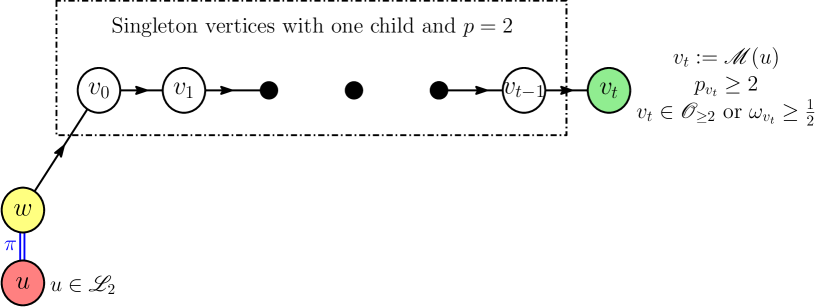
(d) $u\in\mathscr{L}_{2}$ (Case 3).

Figure 8: Construction of $\mathscr{M}$. Vertices in the same block of $\pi$ are connected with blue double edges $(\overset{\text{\tiny{$\pi$}}}{=\joinrel=})$. Vertex colors do not represent blocks of $\pi$.

Proof.

We first describe the construction of $\mathscr{M}$. We consider 4 cases $u\in\mathscr{B}_{1}$, $u\in\mathscr{B}_{2}$, $u\in\mathscr{L}_{2}$ and $u\in\mathscr{L}_{3}$.

1. $u\in\mathscr{B}_{1}$: In this case we know that $u\in V\backslash B_{1}$ with $p_{u}=1$, $c_{u}=1$ and $|B_{\pi(u)}|=1$. By the Parity Property, we know that $q_{u}\notin\{0,2\}$. Furthermore by Forbidden Weights Property, $q_{u}\neq 1$. Hence, $q_{u}\geq 3$. Let $v$ denote the unique child of $u$. By the conservation constraint (45), we must have $p_{v}\geq 3$. This also means that $\omega_{v}\geq 1/2$ (cf. (69)), and in particular $v\in\mathscr{E}$. We set $\mathscr{M}(u)\mathrel{\mathop{\ordinarycolon}}=v$, which verifies claim (1). This case is depicted in Figure 8(a).

2. $u\in\mathscr{B}_{2}$: In this case we know that $u\in V\backslash B_{1}$ with $p_{u}=1,|B_{\pi(u)}|=1$ and $c_{u}=2$. By the same argument as the previous case, we must have $q_{u}\not\in\{0,1,2\}$. Hence $q_{u}\geq 3$. Since $u$ has exactly two children, by the conservation constraint (45), it has a child $v_{0}$ with $p_{v_{0}}\geq 2$. Now by Lemma 15, there is a $t\in\mathbb{N}_{0}$ and a path $v_{0}\rightarrow v_{1}\rightarrow\dotsb\rightarrow v_{t}$ with the following properties:

   1. $v_{i}\in V\backslash B_{1},\;p_{v_{i}}=2,\;|B_{\pi(v_{i})}|=1,\;c_{v_{i}}=1$ for all $0\leq i\leq t-1$.

   2. $v_{t}\in V\backslash\mathscr{R}(F)$ with $p_{v_{t}}\geq 2$.

   3. Exactly one of the following is true:

      1. $\omega_{v_{t}}\geq 1/2$

      2. $v_{t}\in V\backslash B_{1}$ and $p_{v_{t}}=2,|B_{\pi(v_{t})}|=1,c_{v_{t}}\geq 2$.

   We set $\mathscr{M}(u)\mathrel{\mathop{\ordinarycolon}}=v_{t}$ and observe that $p_{v_{t}}\geq 2$ and either $v_{t}\in\mathscr{E}$ with $\omega_{v_{t}}\geq 1/2$ or $v_{t}\in\mathscr{O}_{\geq 2}\backslash B_{1}$ with $p_{v_{t}}=2,|B_{\pi(v_{t})}|=1,c_{v_{t}}\geq 2$, as claimed. This case is depicted in Figure 8(c).

3. $u\in\mathscr{L}_{2}$: In this case, we know that $u\in\mathscr{L}(F)\backslash B_{1}$ with $p_{u}=1,B_{\pi(u)}=\{u,w\}$ where $w\in V\backslash B_{1}$ satisfies $p_{w}=1,c_{w}=1$. By the conservation constraint $q_{w}\neq 0$. By the Parity Property, $q_{w}\neq 1$ (since $p_{u}+p_{w}+q_{w}$ has even parity). Hence we must $q_{w}\geq 2$. Let $v_{0}$ be the unique child of $w$. By the conservation constraint (45), $p_{v_{0}}\geq 2$. Now by Lemma 15, there is a $t\in\mathbb{N}_{0}$ and a path $v_{0}\rightarrow v_{1}\rightarrow\dotsb\rightarrow v_{t}$ with the following properties:

   1. $v_{i}\in V\backslash B_{1},\;p_{v_{i}}=2,\;|B_{\pi(v_{i})}|=1,\;c_{v_{i}}=1$ for all $0\leq i\leq t-1$.

   2. $v_{t}\in V\backslash\mathscr{R}(F)$ with $p_{v_{t}}\geq 2$.

   3. Exactly one of the following is true:

      1. $\omega_{v_{t}}\geq 1/2$

      2. $v_{t}\in V\backslash B_{1}$ and $p_{v_{t}}=2,|B_{\pi(v_{t})}|=1,c_{v_{t}}\geq 2$.

   We set $\mathscr{M}(u)\mathrel{\mathop{\ordinarycolon}}=v_{t}$ and observe that $p_{v_{t}}\geq 2$ and either $v_{t}\in\mathscr{E}$ with $\omega_{v_{t}}\geq 1/2$ or $v_{t}\in\mathscr{O}_{\geq 2}\backslash B_{1}$ with $p_{v_{t}}=2,|B_{\pi(v_{t})}|=1,c_{v_{t}}\geq 2$, as claimed. This case is depicted in Figure 8(d).

4. If $u\in\mathscr{L}_{3}$, then we know that $u\in\mathscr{L}(F)\backslash B_{1}$ with $p_{u}=1,B_{\pi(u)}=\{u,v\}$ with $v\in V\backslash B_{1}$ and $p_{v}=1$ and $c_{v}\geq 2$. In particular observe that $v\in\mathscr{O}_{\geq 2}$ and hence we can set $\mathscr{M}{(u)}\mathrel{\mathop{\ordinarycolon}}=v$. This case is depicted in Figure 8(b).

Next, we need to show the map defined above is injective. Define the following subset of vertices:

$$\mathcal{S}\overset{\text{\tiny{def}}}{=}\{w\in V\backslash B_{1}\mathrel{\mathop{\ordinarycolon}}p_{w}=2,|B_{\pi(w)}|=1,c_{w}=1\}.$$

Observe that in Figure 8, the vertices in $\mathcal{S}$ are exactly the white vertices. From the construction of $\mathscr{M}$ defined (refer to Figure 8) above we observe the following claims are true:

1. If $v=\mathscr{M}{(u)}$ for some $u\in\mathscr{L}_{3}$ then $p_{v}=1$ and $B_{\pi(v)}=\{u,v\}$. On the other hand, if $v=\mathscr{M}{(u)}$ for some $u\in\mathscr{B}_{1}\cup\mathscr{B}_{2}\cup\mathscr{L}_{2}$, then $p_{v}\geq 2$.

2. If $v=\mathscr{M}{(u)}$ for some $u\in\mathscr{B}_{1}$, then the parent of $v$ is $u$ and $u\not\in\mathcal{S}$. In particular, the closest ancestor of $v$ which is not in the set $\mathcal{S}$ is precisely $u$.

3. If $v=\mathscr{M}{(u)}$ for some $u\in\mathscr{B}_{2}$, then the closest ancestor of $v$ which is not in the set $\mathcal{S}$ is precisely $u$.

4. If $v=\mathscr{M}{(u)}$ for some $u\in\mathscr{L}_{2}$, then the closest ancestor of $v$ which is not in the set $\mathcal{S}$ is an internal node $w$ with the property $p_{w}=1,c_{w}=1,B_{\pi(w)}=\{w,u\}$. Furthermore $w\not\in\mathscr{B}_{1}$ and $w\not\in\mathscr{B}_{2}$.

The above three claims provide an algorithm to compute $\mathscr{M}^{-1}(v)$:

1. If $p_{v}=1$, then it must be that $B_{\pi(v)}=\{u,v\}$ and $\mathscr{M}^{-1}(v)\mathrel{\mathop{\ordinarycolon}}=u$.

2. If $p_{v}\geq 2$, find the closest ancestor of $v$ that is not in the set $\mathcal{S}$. Let this ancestor be $w$.

   • If $w\in\mathscr{B}_{1}$ then, $\mathscr{M}^{-1}(v)\mathrel{\mathop{\ordinarycolon}}=w$.

   • If $w\in\mathscr{B}_{2}$ then, $\mathscr{M}^{-1}(v)\mathrel{\mathop{\ordinarycolon}}=w$.

   • If none of the above conditions are met, then it must be that $B_{\pi(w)}=\{u,w\}$ and $\mathscr{M}^{-1}(v)\mathrel{\mathop{\ordinarycolon}}=u$.

Since we have constructed an inverse for $\mathscr{M}$, $\mathscr{M}$ is injective. ∎

9.3 Proof of Proposition 5

Proof of Proposition 5.

We are now ready to prove for Proposition 5. It relies on several results proved previously, which we reproduce below for convenience.

1. In Lemma 14, we showed that,

   $$\eta(F,\pi) \geq\frac{|\mathscr{R}(F)|-|\mathscr{R}_{0}(F)|}{4}+\frac{|\mathscr{O}_{\geq 2}|}{4}-\frac{(|\mathscr{L}_{e}|+|\mathscr{L}_{g}|+|\mathscr{L}_{1}|+|\mathscr{L}_{2}|+|\mathscr{L}_{3}|+|\mathscr{B}_{2}|)}{4}-\frac{|\mathscr{B}_{1}|}{2}+\sum_{v\in\mathscr{O}\cup\mathscr{G}\cup\mathscr{E}}\omega_{v},$$ (72)

   where,

   $$\omega_{v}\overset{\text{\tiny{def}}}{=}\begin{cases}\frac{p_{v}}{2}-\frac{1}{|B_{\pi(v)}|}&\mathrel{\mathop{\ordinarycolon}}v\in V\backslash B_{1}\\ \frac{p_{v}}{2}&\mathrel{\mathop{\ordinarycolon}}v\in B_{1}\backslash\mathscr{R}(F)\\ 0&\mathrel{\mathop{\ordinarycolon}}v\in\mathscr{R}(F)\end{cases}$$ (73)

2. In Lemma 16, we constructed an injective map $\mathscr{M}\mathrel{\mathop{\ordinarycolon}}\mathscr{B}_{1}\cup\mathscr{B}_{2}\cup\mathscr{L}_{2}\cup\mathscr{L}_{3}\rightarrow\mathscr{E}\cup\mathscr{O}_{\geq 2}\backslash\mathscr{R}(F)$ with the following properties:

   1. If $u\in\mathscr{B}_{1}$, then $v\overset{\text{def}}{=}\mathscr{M}(u)$ satisfies $v\in\mathscr{E}$ with $p_{v}\geq 3$.

   2. If $u\in\mathscr{B}_{2}\cup\mathscr{L}_{2}$, then $v\overset{\text{def}}{=}\mathscr{M}(u)$ satisfies $v\in V\backslash\mathscr{R}(F)$ with $p_{v}\geq 2$ and exactly one of the following properties:

      1. $v\in\mathscr{E}$ with $\omega_{v}\geq 1/2$.

      2. $v\in\mathscr{O}_{\geq 2}\backslash B_{1}$ with $p_{v}=2,\;|B_{\pi(v)}|=1,c_{v}\geq 2$.

   3. If $u\in\mathscr{L}_{3}$, then $v\overset{\text{def}}{=}\mathscr{M}(u)$ satisfies $v\in\mathscr{O}_{\geq 2}\backslash B_{1}$ with $p_{v}=1,|B_{\pi(v)}|=2$ and $c_{v}\geq 2$.

As mentioned previously, the rational of constructing the map $\mathscr{M}$ is to cancel the negative contribution of a vertex $u\in\mathscr{B}_{1}\cup\mathscr{B}_{2}\cup\mathscr{L}_{2}\cup\mathscr{L}_{3}$ in the lower bound in (72) by the positive effect of $\mathscr{M}({u})\in\mathscr{O}_{\geq 2}\cup\mathscr{E}$. To this end, we make the following observations. First, we observe that we can partition the sets $\mathscr{B}_{2}$ and $\mathscr{L}_{2}$ as $\mathscr{B}_{2}=\mathscr{B}_{2}^{o}\cup\mathscr{B}_{2}^{e}$ and $\mathscr{L}_{2}=\mathscr{L}_{2}^{o}\cup\mathscr{L}_{2}^{e}$ where:

$$\mathscr{B}_{2}^{o} =\{u\in\mathscr{B}_{2}\mathrel{\mathop{\ordinarycolon}}\mathscr{M}(u)\in\mathscr{O}_{\geq 2}\},\;\mathscr{B}_{2}^{e}=\{u\in\mathscr{B}_{2}\mathrel{\mathop{\ordinarycolon}}\mathscr{M}(u)\in\mathscr{E}\},$$

$$\mathscr{L}_{2}^{o} =\{u\in\mathscr{L}_{2}\mathrel{\mathop{\ordinarycolon}}\mathscr{M}(u)\in\mathscr{O}_{\geq 2}\},\;\mathscr{L}_{2}^{e}=\{u\in\mathscr{L}_{2}\mathrel{\mathop{\ordinarycolon}}\mathscr{M}(u)\in\mathscr{E}\}$$

By the injectivity of $\mathscr{M}$, $|\mathscr{B}_{2}^{o}|+|\mathscr{L}_{2}^{o}|+|\mathscr{L}_{3}|\leq|\mathscr{O}_{\geq 2}|$. Hence,

$$\eta(F,\pi) \geq\frac{|\mathscr{R}(F)|-|\mathscr{R}_{0}(F)|}{4}-\frac{(|\mathscr{L}_{e}|+|\mathscr{L}_{g}|+|\mathscr{L}_{1}|+|\mathscr{L}_{2}^{e}|+|\mathscr{B}_{2}^{e}|)}{4}-\frac{|\mathscr{B}_{1}|}{2}+\sum_{v\in\mathscr{O}\cup\mathscr{G}\cup\mathscr{E}}\omega_{v}$$

Next, we transfer the negative contribution of a vertex $u\in\mathscr{B}_{2}^{e}\cup\mathscr{L}_{2}^{e}\cup\mathscr{B}_{1}$ to $\mathscr{M}(u)$ by defining weights $\mu_{v}$ for each $v\in V$ as follows:

$$\mu_{v} =\begin{cases}2&\mathrel{\mathop{\ordinarycolon}}v\in\mathscr{M}(\mathscr{B}_{1})\\ 1&\mathrel{\mathop{\ordinarycolon}}v\in\mathscr{M}(\mathscr{B}_{2}\cup\mathscr{L}_{2})\cap\mathscr{E}\\ 0&\mathrel{\mathop{\ordinarycolon}}\text{ otherwise}\end{cases}.$$

The injectivity of $\mathscr{M}$ again guarantees:

$$\eta(F,\pi) \geq\frac{|\mathscr{R}(F)|-|\mathscr{R}_{0}(F)|}{4}+\sum_{v\in\mathscr{O}\cup\mathscr{G}\cup\mathscr{E}}\left(\omega_{v}-\frac{\mu_{v}}{4}\right)-\frac{(|\mathscr{L}_{e}|+|\mathscr{L}_{g}|+|\mathscr{L}_{1}|)}{4}.$$ (74)

We also record the following implications that we use several times in the proof:

$$\mu_{v}=1 \implies\omega_{v}\geq 1/2 \text{[follows from Lemma~{}\ref{lem:map-construction} recalled in item (2b) above]},$$ (75a)

$$\mu_{v}=2 \implies p_{v}\geq 3\implies\omega_{v}\geq 3/2-1=1/2 \text{[follows from Lemma~{}\ref{lem:map-construction} recalled in (2a) and \eqref{eq:effect-def-recall}]}.$$ (75b)

We further rewrite (74) by defining the weights:

$$\lambda_{v} =\begin{cases}1&\mathrel{\mathop{\ordinarycolon}}v\in\mathscr{L}_{e}\cup\mathscr{L}_{g}\cup\mathscr{L}_{1}\\ 0&\mathrel{\mathop{\ordinarycolon}}\text{ otherwise}\end{cases},$$

Since $\mathscr{L}_{e}\cup\mathscr{L}_{g}\cup\mathscr{L}_{1}\subset\mathscr{O}\cup\mathscr{G}\cup\mathscr{E}$ we can rexpress (74) as:

$$\eta(F,\pi) \geq\frac{|\mathscr{R}(F)|-|\mathscr{R}_{0}(F)|}{4}+\sum_{v\in\mathscr{O}\cup\mathscr{G}\cup\mathscr{E}}\left(\omega_{v}-\frac{\mu_{v}}{4}-\frac{\lambda_{v}}{4}\right).$$

In order to show that $\eta(F,\pi)\geq(|\mathscr{R}(F)|-|\mathscr{R}_{0}(F)|)/4$, we will show that,

$$\sum_{v\in\mathscr{O}\cup\mathscr{G}\cup\mathscr{E}}\left(\omega_{v}-\frac{\mu_{v}}{4}-\frac{\lambda_{v}}{4}\right)\geq 0.$$

In order to show the above inequality, for each node $u\in\mathscr{O}\cup\mathscr{G}\cup\mathscr{E}$, we will show that either,

$$\omega_{u}-\frac{\mu_{u}}{4}-\frac{\lambda_{u}}{4}\geq 0,$$

or for $B\mathrel{\mathop{\ordinarycolon}}=B_{\pi(u)}$,

$$\sum_{v\in(\mathscr{O}\cup\mathscr{G}\cup\mathscr{E})\cap B}\left(\omega_{v}-\frac{\mu_{v}}{4}-\frac{\lambda_{v}}{4}\right)\geq 0.$$

We consider the following 4 exhaustive cases for $u$: $\lambda_{u}=0$ or $\lambda_{u}=1,\mu_{u}=0$ or $\lambda_{u}=1,\mu_{u}=1$ or $\lambda_{u}=1,\mu_{u}=2$.

1. $\lambda_{u}=0\mathrel{\mathop{\ordinarycolon}}$ In this case if $\mu_{u}=0$, we know by Definition 14, that for any $u\in\mathscr{O}\cup\mathscr{G}\cup\mathscr{E}$,

   $$\omega_{u}\geq 0\implies\omega_{u}-\frac{\mu_{u}}{4}-\frac{\lambda_{u}}{4}\geq 0.$$

   On the other hand if $\mu_{u}\geq 1$, (75) guarantees that,

   $$\omega_{u}\geq 1/2\implies\omega_{u}-\frac{\mu_{u}}{4}-\frac{\lambda_{u}}{4}\geq 0.$$

2. $\lambda_{u}=1,\mu_{u}=1$: In this case, (75) yields:

   $$\omega_{u}\geq 1/2\implies\omega_{u}-\frac{\mu_{u}}{4}-\frac{\lambda_{u}}{4}\geq 0.$$

3. $\lambda_{u}=1,\mu_{u}=2$: In this case, we know that $u$ is a leaf and furthermore by (75) $p_{u}\geq 3$. We consider the following two sub-cases:

   1. $|B_{\pi(u)}|=1$. In this case, by the Parity Property we cannot have $p_{u}=3$. Hence, we must have, $p_{u}\geq 4$. And hence,

      $$\omega_{u}-\frac{\mu_{u}}{4}-\frac{\lambda_{u}}{4}\geq\frac{p_{u}}{2}-\frac{1}{|B_{\pi(u)}|}-\frac{\mu_{u}}{4}-\frac{\lambda_{u}}{4}\geq 2-1-\frac{2}{4}-\frac{1}{4}=\frac{1}{4}.$$

   2. $|B_{\pi(u)}|\geq 2$. In this case, we have,

      $$\omega_{u}-\frac{\mu_{u}}{4}-\frac{\lambda_{u}}{4}\geq\frac{p_{u}}{2}-\frac{1}{|B_{\pi(u)}|}-\frac{\mu_{u}}{4}-\frac{\lambda_{u}}{4}\geq\frac{3}{2}-\frac{1}{2}-\frac{2}{4}-\frac{1}{4}=\frac{1}{4}.$$

4. $\lambda_{u}=1,\mu_{u}=0$: In this case, we already know that $u\in\mathscr{L}_{e}\cup\mathscr{L}_{1}\cup\mathscr{L}_{g}$. We consider 3 exhaustive sub-cases corresponding to whether $u\in\mathscr{L}_{e}$ or $u\in\mathscr{L}_{1}$ or $u\in\mathscr{L}_{g}$.

   1. $u\in\mathscr{L}_{e}$: In this case the definition of excellent leaves (Definition 15) guarantees:

      $$\omega_{u}\geq 1/4\implies\omega_{u}-\frac{\mu_{u}}{4}-\frac{\lambda_{u}}{4}\geq 0.$$

   2. $u\in\mathscr{L}_{1}$: In this case, we know that $u\in\mathscr{L}(F)\backslash B_{1}$ with $p_{u}=1,B_{\pi(u)}=\{u,v\}$ for some node $v\in V\backslash B_{1}$ with $p_{v}\geq 2$. In this case we will show that for $B=B_{\pi(u)}=\{u,v\}$ we have,

      $$\left(\omega_{u}-\frac{\mu_{u}}{4}-\frac{\lambda_{u}}{4}\right)+\left(\omega_{v}-\frac{\mu_{v}}{4}-\frac{\lambda_{v}}{4}\right) =\left(\frac{p_{u}}{2}-\frac{1}{|B_{\pi(u)}|}-\frac{\mu_{u}}{4}-\frac{\lambda_{u}}{4}\right)+\left(\frac{p_{v}}{2}-\frac{1}{|B_{\pi(v)}|}-\frac{\mu_{v}}{4}-\frac{\lambda_{v}}{4}\right)$$

      $$=\frac{p_{v}}{2}-\frac{3}{4}-\frac{\lambda_{v}+\mu_{v}}{4}$$

      We consider two sub-cases depending on whether $v$ is a leaf or not.

      1. $v$ is a leaf: Then by the Parity Property, $p_{u}+p_{v}$ must be even and so infact, $p_{v}\geq 3$. Since $\lambda_{v}+\mu_{v}\leq 3$, we have,

         $$\frac{p_{v}}{2}-\frac{3}{4}-\frac{\lambda_{v}+\mu_{v}}{4}\geq 0.$$

      2. $v$ is not a leaf: Note that $\lambda_{v}=0$. If $\mu_{v}\leq 1$, then again since we know $p_{v}\geq 2$,

         $$\frac{p_{v}}{2}-\frac{3}{4}-\frac{\lambda_{v}+\mu_{v}}{4}\geq 0.$$

         On the other hand if $\mu_{v}=2$, then (75) guarantees $p_{v}\geq 3$. Hence,

         $$\frac{p_{v}}{2}-\frac{3}{4}-\frac{\lambda_{v}+\mu_{v}}{4}\geq\frac{1}{4}.$$

   3. $u\in\mathscr{L}_{g}\mathrel{\mathop{\ordinarycolon}}$ In this case, from the definition of good leaves (Definition 15), we know that $u\in\mathscr{L}(F)\backslash B_{1}$ with $p_{u}=1$ and $B_{\pi(u)}=\{u,v,w\}$. Since $B_{1}$ and $B_{\pi(u)}$ are both blocks of a partition, they must either be identical or disjoint. Since $u\not\in B_{1}$, $B_{1}$ and $B_{\pi(u)}$ must be disjoint. Hence, $v,w\in V\backslash B_{1}$. Consequently, recalling the definition of $\omega$ from (73) in this case, we need to show,

      $$\left(\omega_{u}-\frac{\mu_{u}}{4}-\frac{\lambda_{u}}{4}\right)+\left(\omega_{v}-\frac{\mu_{v}}{4}-\frac{\lambda_{v}}{4}\right)+\left(\omega_{w}-\frac{\mu_{w}}{4}-\frac{\lambda_{w}}{4}\right)=$$

      $$\left(\frac{p_{u}}{2}-\frac{1}{|B_{\pi(u)}|}-\frac{\mu_{u}}{4}-\frac{\lambda_{u}}{4}\right)+\left(\frac{p_{v}}{2}-\frac{1}{|B_{\pi(v)}|}-\frac{\mu_{v}}{4}-\frac{\lambda_{v}}{4}\right)+\left(\frac{p_{w}}{2}-\frac{1}{|B_{\pi(w)}|}-\frac{\mu_{w}}{4}-\frac{\lambda_{w}}{4}\right)\geq 0.$$

      Since we know $p_{u}=1,B_{\pi(u)}=\{u,v,w\},\lambda_{u}=1,\mu_{u}=0$ we can simplify the above formula and we need to show:

      $$\frac{1+p_{v}+p_{w}}{2}-1-\frac{1+\lambda_{v}+\lambda_{w}}{4}-\frac{\mu_{v}+\mu_{w}}{4}\geq 0.$$ (76)

      We will consider the following 4 exhaustive cases:

      1. $(\mu_{v}\geq 1,\mu_{w}\geq 1)$: Observe that since $\mu_{v}\geq 1$, the construction of $\mathscr{M}$ guarantees (cf. (75)):

         $$\omega_{v}=\frac{p_{v}}{2}-\frac{1}{|B_{\pi(v)}|}\geq\frac{1}{2}\implies p_{v}\geq\frac{5}{3}\implies p_{v}\geq 2.$$

         Analogously, we can argue that $p_{w}\geq 2$. If there are at most $2$ leaves among $\{u,v,w\}$ (and hence $\lambda_{u}+\lambda_{v}+\lambda_{w}\leq 2)$, we can lower bound (76) as follows:

         $$\frac{1+p_{v}+p_{w}}{2}-1-\frac{1+\lambda_{v}+\lambda_{w}}{4}-\frac{\mu_{v}+\mu_{w}}{4}\geq\frac{5}{2}-1-\frac{2}{4}-\frac{4}{4}\geq 0.$$

         On the other hand, if all 3 of $\{u,v,w\}$ are leaves, by the Parity Property, we must have $p_{u}+p_{v}+p_{w}$ is even. Since we know that $p_{u}+p_{v}+p_{w}\geq 5$ we must in fact have $p_{u}+p_{v}+p_{w}\geq 6$. We can now lower bound (76) as follows:

         $$\frac{1+p_{v}+p_{w}}{2}-1-\frac{1+\lambda_{v}+\lambda_{w}}{4}-\frac{\mu_{v}+\mu_{w}}{4}\geq\frac{6}{2}-1-\frac{3}{4}-\frac{4}{4}\geq\frac{1}{4}.$$

      2. $(\mu_{v}=2,\mu_{w}=0)$ or $(\mu_{v}=0,\mu_{w}=2)$: Observe that these cases are symmetric. Hence we only need to consider the case $(\mu_{v}=2,\mu_{w}=0)$. In this situation, the construction of $\mathscr{M}$ guarantees $p_{v}\geq 3$ (cf. (75)). Additionally we have, $p_{w}\geq 1$ and $\lambda_{v}+\lambda_{w}\leq 2$ and $\mu_{v}+\mu_{w}=2$. Hence, we can now lower bound (76) as follows:

         $$\frac{1+p_{v}+p_{w}}{2}-1-\frac{1+\lambda_{v}+\lambda_{w}}{4}-\frac{\mu_{v}+\mu_{w}}{4}\geq\frac{5}{2}-1-\frac{3}{4}-\frac{2}{4}\geq\frac{1}{4}.$$

      3. $(\mu_{v}=1,\mu_{w}=0)$ or $(\mu_{v}=0,\mu_{w}=1)$: Observe that these cases are symmetric. Hence we only need to consider the case $(\mu_{v}=1,\mu_{w}=0)$. In this situation, since $\mu_{v}=1$, the construction of $\mathscr{M}$ guarantees (cf. (75)):

         $$\omega_{v}=\frac{p_{v}}{2}-\frac{1}{|B_{\pi(v)}|}\geq\frac{1}{2}\implies p_{v}\geq\frac{5}{3}\implies p_{v}\geq 2.$$

         Hence, by observing $p_{w}\geq 1,\lambda_{v}+\lambda_{w}\leq 2$ and $\mu_{v}+\mu_{w}=1$ we can now lower bound (76) as follows:

         $$\frac{1+p_{v}+p_{w}}{2}-1-\frac{1+\lambda_{v}+\lambda_{w}}{4}-\frac{\mu_{v}+\mu_{w}}{4}\geq\frac{4}{2}-1-\frac{3}{4}-\frac{1}{4}\geq 0.$$

      4. $(\mu_{v}=0,\mu_{w}=0)$: Observe that since $p_{v}\geq 1$ and $p_{w}\geq 1$ we have $p_{u}+p_{v}+p_{w}\geq 3$. Furthermore, $\mu_{v}+\mu_{w}=0$. Now if there are at most $2$ leaves among $\{u,v,w\}$, we have $\lambda_{u}+\lambda_{v}+\lambda_{w}\leq 2$ and hence we can lower bound (76) as follows:

         $$\frac{1+p_{v}+p_{w}}{2}-1-\frac{1+\lambda_{v}+\lambda_{w}}{4}-\frac{\mu_{v}+\mu_{w}}{4}\geq\frac{3}{2}-1-\frac{2}{4}-\frac{0}{4}\geq 0.$$

         On the other hand, if all 3 of $\{u,v,w\}$ are leaves, by the Parity Property $p_{u}+p_{v}+p_{w}$ is even. Since $p_{u}+p_{v}+p_{w}\geq 3$, we infact have $p_{u}+p_{v}+p_{w}\geq 4$. Hence we obtain the following lower bound on (76):

         $$\frac{1+p_{v}+p_{w}}{2}-1-\frac{1+\lambda_{v}+\lambda_{w}}{4}-\frac{\mu_{v}+\mu_{w}}{4}\geq\frac{4}{2}-1-\frac{3}{4}-\frac{0}{4}\geq\frac{1}{4}.$$

This concludes the proof. ∎

10 Proof of Theorem 2

In this section, we provide a proof for Theorem 2. Using a simple rescaling argument, we can without loss of generality assume that the matrix ensemble $\boldsymbol{M}$ is semi-random with $\sigma_{\psi}^{2}=1$ (Definition 1), the initialization ${\boldsymbol{z}}^{(0)}\sim\mathcal{N}\left(0,1\right)$ (that is, Assumption 1 holds with $\sigma_{0}^{2}=1$) and the non-linearities satisfy $\mathbb{E}f_{t}^{2}(Z)=1$ for $t\;\in\;[T]$ and $Z\sim\mathcal{N}\left(0,1\right)$. We record this rescaling argument in the lemma below and defer its proof to Appendix C for the reader interested in the full details.

Lemma 17 (Rescaling).

It is sufficient to prove Theorem 2 under the additional assumptions: (a) the matrix ensemble $\boldsymbol{M}$ is semi-random with $\sigma_{\psi}^{2}=1$ (Definition 1), (b) the initialization ${\boldsymbol{z}}^{(0)}\sim\mathcal{N}\left(0,1\right)$ (that is, Assumption 1 holds with $\sigma_{0}^{2}=1$) and, (c) the non-linearities satisfy $\mathbb{E}f_{t}^{2}(Z)=1$ for $t\;\in\;[T]$ and $Z\sim\mathcal{N}\left(0,1\right)$.

Theorem 3 will play a critical role in our proof. We first complement Theorem 3 with the following concentration estimate.

Theorem 4.

Under the assumptions of Theorem 3, for any polynomial test function $h\mathrel{\mathop{\ordinarycolon}}\mathbb{R}^{t+1}\rightarrow\mathbb{R}$ with degree at most $D$, we have,

$$\mathrm{Var}\left[\frac{1}{N}\sum_{i=1}^{N}h({\boldsymbol{z}}^{(0)}_{i},{\boldsymbol{z}}^{(1)}_{i},\dotsc,{\boldsymbol{z}}^{(t)}_{i})\right] \lesssim N^{-1+\epsilon}.$$

Proof.

This variance bound is derived using the Efron-Stein Inequality [27]. The complete derivation is provided in Appendix D for the interested reader. ∎

In order to deduce Theorem 2 from Theorem 3, we will rely on the following approximation result, which shows that an iteration which satisfies the assumptions of Theorem 2 can always be approximated by an iteration which satisfies the assumptions of Theorem 3.

Proposition 6 (Approximation).

Fix a non-negative integer $T\in\mathbb{N}_{0}$ and functions $f_{1},f_{2},\dotsc,f_{T}\mathrel{\mathop{\ordinarycolon}}\mathbb{R}\rightarrow\mathbb{R}$ and a test function $h\mathrel{\mathop{\ordinarycolon}}\mathbb{R}^{T+1}\rightarrow\mathbb{R}$. Consider the iteration:

$${\boldsymbol{z}}^{(t+1)}=\boldsymbol{M}f_{t+1}({\boldsymbol{z}}^{(t)}),$$

initialized at ${\boldsymbol{z}}^{(0)}$ that satisfies the assumptions of Theorem 2 with constants $\sigma_{\psi}^{2}=1$ and $\sigma_{0}^{2}=1$. Suppose that the test function $h$ satisfies the following continuity estimate for some fixed constant $L\geq 0$:

$$|h(\boldsymbol{x})-h(\boldsymbol{x}^{\prime})| \leq L\cdot\|\boldsymbol{x}-\boldsymbol{x}^{\prime}\|\cdot(1+\|\boldsymbol{x}\|+\|\boldsymbol{x}^{\prime}\|),$$

Then, there is a matrix ensemble $\hat{\boldsymbol{M}}$ and sequences of polynomial approximating functions ${f}^{(k)}_{1},{f}^{(k)}_{2},\dotsc,{f}^{(k)}_{T}\mathrel{\mathop{\ordinarycolon}}\mathbb{R}\rightarrow\mathbb{R}$ and ${h}^{(k)}\mathrel{\mathop{\ordinarycolon}}\mathbb{R}^{T+1}\rightarrow\mathbb{R}$ indexed by $k\in\mathbb{N}$ such that for each $k\in\mathbb{N}$, the iteration:

$${\hat{\boldsymbol{z}}}^{(t+1;k)}=\hat{\boldsymbol{M}}{f}^{(k)}_{t+1}({\hat{\boldsymbol{z}}}^{(t;k)}),$$

initialized at ${\hat{\boldsymbol{z}}}^{(0;k)}={\boldsymbol{z}}^{(0)}$ satisfies the assumptions of Theorem 3 and,

$$\lim_{k\rightarrow\infty}\limsup_{N\rightarrow\infty}\mathbb{E}\left[\left|\frac{1}{N}\sum_{i=1}^{N}h({z}^{(0)}_{i},{z}^{(1)}_{i},\dotsc,{z}^{(T)}_{i})-\frac{1}{N}\sum_{i=1}^{N}{h}^{(k)}({\hat{z}}^{(0;k)}_{i},{\hat{z}}^{(1;k)}_{i},\dotsc,{\hat{z}}^{(T;k)}_{i})\right|\right] =0.$$

The proof of this result is based on routine approximation arguments and is presented in Appendix E. We now present the proof of Theorem 2.

Proof of Theorem 2.

Consider an iteration that satisfies the assumptions of Theorem 2 and the additional assumptions described in Lemma 17:

$${\boldsymbol{z}}^{(t+1)}=\boldsymbol{M}f_{t+1}({\boldsymbol{z}}^{(t)}).$$

with initialization ${\boldsymbol{z}}^{(0)}\sim\mathcal{N}\left(0,1\right)$. In order to understand the dynamics of the above iteration, we will compare it to another iteration which uses a rotationally invariant matrix instead of $\boldsymbol{M}$. The dynamics of such iterations are well-understood from prior work. Specifically, we consider the iteration:

$${\boldsymbol{w}}^{(t+1)}=\boldsymbol{Q}f_{t+1}({\boldsymbol{w}}^{(t)}),$$

with

$$\boldsymbol{Q}=\boldsymbol{S}\boldsymbol{U}\boldsymbol{P}\boldsymbol{\Lambda}\boldsymbol{P}^{\mkern-1.5mu\mathsf{T}}\boldsymbol{U}^{\mkern-1.5mu\mathsf{T}}\boldsymbol{S},$$ (77)

where:

1. ${\boldsymbol{S}}=\operatorname{diag}(s_{1},s_{2},\dotsc,s_{N})$ with $s_{i}\overset{\text{\tiny{i.i.d.}}}{\sim}\mathsf{Unif}(\{\pm 1\})$

2. $\boldsymbol{U}\sim\mathsf{Unif}(\mathbb{O}(N))$.

3. $\boldsymbol{P}$ is a uniformly random $N\times N$ permutation matrix.

4. $\boldsymbol{\Lambda}=\operatorname{diag}(\lambda_{1},\lambda_{2},\dotsc,\lambda_{N})$ with $\lambda_{i}\overset{\text{\tiny{i.i.d.}}}{\sim}\mathsf{Unif}(\{\pm 1\})$.

This choice of $\boldsymbol{Q}$ has two useful properties:

1. $\boldsymbol{Q}$ satisfies is semi-random with constant $\sigma_{\psi}^{2}=1$ in the sense of Definition 1 (cf. Lemma 2).

2. Since the Haar measure on the orthogonal group is invariant to left and right multiplication by orthogonal matrices, $\boldsymbol{Q}\overset{\text{\tiny{d}}}{=}\boldsymbol{U}\boldsymbol{\Lambda}\boldsymbol{U}^{\mkern-1.5mu\mathsf{T}}$. Matrices of the form with $\boldsymbol{U}\boldsymbol{\Lambda}\boldsymbol{U}^{\mkern-1.5mu\mathsf{T}}$ are called rotationally invariant matrices and the dynamics of approximate message passing algorithms for rotationally invariant ensembles has been studied in prior work. In particular, Fan [30, Corollary 4.4] yields the result (see for e.g. Fan and Wu [31, Appendix A] for additional details):

   $$\frac{1}{N}\sum_{i=1}^{N}h({w}^{(0)}_{i},{w}^{(1)}_{i},\dotsc,{w}^{(T)}_{i})\overset{\text{\tiny{P}}}{\rightarrow}\mathbb{E}h(Z_{0},Z_{1},\dotsc,Z_{T}),$$

   where the law of the random vector $(Z_{0},Z_{1},\dotsc Z_{T})$ is as defined in Theorem 2.

As a consequence, Theorem 2 follows if we can show that the random variables:

$$X_{N} \overset{\text{\tiny{def}}}{=}\frac{1}{N}\sum_{i=1}^{N}h({z}^{(0)}_{i},{z}^{(1)}_{i},\dotsc,{z}^{(T)}_{i}),$$

$$Y_{N} \overset{\text{\tiny{def}}}{=}\frac{1}{N}\sum_{i=1}^{N}h({w}^{(0)}_{i},{w}^{(1)}_{i},\dotsc,{w}^{(T)}_{i})$$

satisfy $X_{N}-Y_{N}\overset{\text{\tiny{P}}}{\rightarrow 0}$. In order to show this we use Proposition 6 to construct two sequences of approximating iterations ${\hat{\boldsymbol{z}}}^{(t;k)},{\hat{\boldsymbol{w}}}^{(t;k)}$ and a sequence of approximating polynomial test functions ${h}^{(k)}\mathrel{\mathop{\ordinarycolon}}\mathbb{R}^{T+1}\rightarrow\mathbb{R}$ indexed by $k\in\mathbb{N}$ such that the random variables:

$${X}^{(k)}_{N} \overset{\text{\tiny{def}}}{=}\frac{1}{N}\sum_{i=1}^{N}{h}^{(k)}({\hat{z}}^{(0;k)}_{i},{\hat{z}}^{(1;k)}_{i},\dotsc,{\hat{z}}^{(T;k)}_{i}),$$

$${Y}^{(k)}_{N} \overset{\text{\tiny{def}}}{=}\frac{1}{N}\sum_{i=1}^{N}{h}^{(k)}({\hat{w}}^{(0;k)}_{i},{\hat{w}}^{(1;k)}_{i},\dotsc,{\hat{w}}^{(T;k)}_{i}),$$

approximate $X_{N},Y_{N}$ in the sense:

$$\lim_{k\rightarrow\infty}\limsup_{N\rightarrow\infty}\mathbb{E}\;|X_{N}-{X}^{(k)}_{N}|=\lim_{k\rightarrow\infty}\limsup_{N\rightarrow\infty}\mathbb{E}\;|Y_{N}-{Y}^{(k)}_{N}|=0.$$ (78)

Furthermore, since Proposition 6 guarantees that for each $k\in\mathbb{N}$, the two iterations ${\hat{\boldsymbol{z}}}^{(t;k)},{\hat{\boldsymbol{w}}}^{(t;k)}$ satisfy the requirements of Theorem 3 and Theorem 4 and since ${h}^{(k)}$ is a polynomial,

$$\lim_{N\rightarrow\infty}\mathbb{E}[{X}^{(k)}_{N}] =\lim_{N\rightarrow\infty}\mathbb{E}[{Y}^{(k)}_{N}]\;\forall\;k\;\in\mathbb{N},$$

$$\lim_{N\rightarrow\infty}\mathrm{Var}[{X}^{(k)}_{N}] =\lim_{N\rightarrow\infty}\mathrm{Var}[{Y}^{(k)}_{N}]=0\;\forall\;k\;\in\mathbb{N}.$$

By Chebychev’s Inequality, we have,

$${X}^{(k)}_{N}-{Y}^{(k)}_{N}\overset{\text{\tiny{P}}}{\rightarrow}0\;\forall\;k\;\in\mathbb{N}.$$ (79)

With these observations in hand, we can conclude the claim of the proposition. For any $\epsilon>0$ we have,

$$\lim_{N\rightarrow\infty}\;\mathbb{P}(|X_{N}-Y_{N}|>3\epsilon) \leq\lim_{k\rightarrow\infty}\lim_{N\rightarrow\infty}\left(\mathbb{P}(|X_{N}-{X}^{(k)}_{N}|>\epsilon)+\mathbb{P}(|Y_{N}-{Y}^{(k)}_{N}|>\epsilon)+\mathbb{P}(|{X}^{(k)}-{Y}^{(k)}_{N}|>\epsilon)\right)$$

$$\overset{\text{\tiny{\eqref{eq:chebychev-conclusion}}}}{=}\lim_{k\rightarrow\infty}\lim_{N\rightarrow\infty}\left(\mathbb{P}(|X_{N}-{X}^{(k)}_{N}|>\epsilon)+\mathbb{P}(|Y_{N}-{Y}^{(k)}_{N}|>\epsilon)\right)$$

$$\leq\lim_{k\rightarrow\infty}\lim_{N\rightarrow\infty}\left(\mathbb{E}\;|X_{N}-{X}^{(k)}_{N}|+\mathbb{E}\;|Y_{N}-{Y}^{(k)}_{N}|\right)/\epsilon$$

$$\overset{\text{\tiny{\eqref{eq:appx-guarantee}}}}{=}0.$$

This concludes the proof of Theorem 3. ∎

Acknowledgements

We are grateful to Giorgio Cipolloni, Jiaoyang Huang, Benjamin Landon, and Dominik Schröder for helpful discussions regarding the local law for Wigner matrices. The work of YML is supported by a Harvard FAS Dean’s competitive fund award for promising scholarship, and by the US National Science Foundation under grant CCF-1910410. SS gratefully acknowledges support from a Harvard FAS Dean’s competitive fund award.

Appendix A Omitted Proofs from Section 1.3

A.1 Proof of Lemma 2

Proof of Lemma 2.

Let $\boldsymbol{S}=\operatorname{diag}{(\boldsymbol{s})},\boldsymbol{s}\sim\mathsf{Unif}(\{\pm 1\}^{N})$ be a uniformly random signed diagonal matrix and $\boldsymbol{P}$ be a uniformly random $N\times N$ permutation matrix independent of each other and independent of $\boldsymbol{F}$. By the assumptions of the lemma, we have, $\boldsymbol{M}\overset{\text{\tiny{d}}}{=}\widetilde{\boldsymbol{M}}\overset{\text{\tiny{d}}}{=}\boldsymbol{S}\boldsymbol{F}\boldsymbol{P}\boldsymbol{\Lambda}\boldsymbol{P}^{\mkern-1.5mu\mathsf{T}}\boldsymbol{F}^{\mkern-1.5mu\mathsf{T}}\boldsymbol{S}$. Let $\boldsymbol{\Psi}$ denote the matrix:

$${\boldsymbol{\Psi}\overset{\text{\tiny{def}}}{=}\boldsymbol{F}\boldsymbol{P}\cdot\boldsymbol{\Lambda}\cdot\boldsymbol{P}^{\mkern-1.5mu\mathsf{T}}\boldsymbol{F}}.$$

As a consequence of the distributional equivalence of $\boldsymbol{M}$ and $\widetilde{\boldsymbol{M}}\overset{\text{\tiny{def}}}{=}\boldsymbol{S}\boldsymbol{\Psi}\boldsymbol{S}$, it is sufficient to verify that $\widetilde{\boldsymbol{M}}$ satisfies the requirements of Definition 1 with probability 1. Note that $\widetilde{\boldsymbol{M}}\overset{\text{\tiny{def}}}{=}\boldsymbol{S}\boldsymbol{\Psi}\boldsymbol{S}$ satisfies item (1) of Definition 1 by construction. In order to verify item (2) of Definition 1 observe that we can write:

$${\boldsymbol{\Psi}} =\mathbb{E}[{\boldsymbol{\Psi}}]+({\boldsymbol{\Psi}}-\mathbb{E}[{\boldsymbol{\Psi}}]),$$

$${{\boldsymbol{\Psi}}}^{2} =\mathbb{E}[{\boldsymbol{\Psi}}^{2}]+({{\boldsymbol{\Psi}}}^{2}-\mathbb{E}[{{\boldsymbol{\Psi}}}^{2}]).$$

Next, we compute $\mathbb{E}[{\boldsymbol{\Psi}}]$ and $\mathbb{E}[{\boldsymbol{\Psi}}^{2}]$, where the expectation is with respect to the randomness in $\boldsymbol{P}$. Let $\tau$ be the uniformly random permutation associated with $\boldsymbol{P}$ and let $\lambda_{1\mathrel{\mathop{\ordinarycolon}}N}$ denote the diagonal entries of $\boldsymbol{\Lambda}$. We have,

$$\mathbb{E}[\psi_{ij}] =\sum_{k=1}^{N}f_{ik}f_{jk}\mathbb{E}[\lambda_{\tau(k)}]=\frac{\operatorname{Tr}(\boldsymbol{\Lambda})}{N}\cdot(\boldsymbol{F}\boldsymbol{F}^{\mkern-1.5mu\mathsf{T}})_{ij}.$$ (80a)

$$\mathbb{E}[(\boldsymbol{\Psi}^{2})_{ij}] =\sum_{k=1}^{N}f_{ik}f_{jk}\mathbb{E}[\lambda_{\tau(k)}^{2}]=\frac{\operatorname{Tr}(\boldsymbol{\Lambda}^{2})}{N}\cdot(\boldsymbol{F}\boldsymbol{F}^{\mkern-1.5mu\mathsf{T}})_{ij}.$$ (80b)

Next, we obtain a concentration estimate for $\|{\boldsymbol{\Psi}}-\mathbb{E}[{\boldsymbol{\Psi}}]\|_{\infty}$ and $\|{\boldsymbol{\Psi}^{2}}-\mathbb{E}[{\boldsymbol{\Psi}^{2}}]\|_{\infty}$. For any matrix $\boldsymbol{A}\in\mathbb{R}^{N\times N}$, Bercu et al. [9, Theorem 4.3] show that the statistic :

$$X_{N}(\boldsymbol{A})\overset{\text{def}}{=}\sum_{\ell=1}^{N}A_{\ell,\tau(\ell)},$$

constructed using a uniformly random permutation $\tau$ satisfies the following concentration estimate for any $\delta\in(0,1/4)$:

$$\mathbb{P}\left(|X_{N}(\boldsymbol{A})-\mathbb{E}X_{N}(\boldsymbol{A})|>\frac{C\cdot\|\boldsymbol{A}\|_{\operatorname{Fr}}}{\sqrt{N}}\cdot\sqrt{\ln\left(\frac{1}{\delta}\right)}+C\cdot\|\boldsymbol{A}\|_{\infty}\ln\left(\frac{1}{\delta}\right)\right) \leq 4\delta,$$

for a suitable constant $0<C<\infty$. Fix any $i,j\in[N]$. We apply the above concentration inequality with the choice $\delta=1/N^{4}$ and $\boldsymbol{A}={\boldsymbol{A}}^{(ij)}$ where the entries of ${\boldsymbol{A}}^{(ij)}$ are ${A}^{(ij)}_{k\ell}\overset{\text{\tiny{def}}}{=}f_{ik}f_{jk}\lambda_{\ell}$. Observe that,

$$X_{N}({\boldsymbol{A}}^{(ij)}) =\psi_{ij},$$

$$\|{\boldsymbol{A}}^{(ij)}\|_{\operatorname{Fr}}^{2} =\left(\sum_{k=1}^{N}f_{ik}^{2}f_{jk}^{2}\right)\cdot\left(\sum_{\ell=1}^{N}\lambda_{\ell}^{2}\right)\leq N^{2}\|\boldsymbol{F}\|_{\infty}^{4}\|\boldsymbol{\Lambda}\|_{\operatorname{op}}^{2},$$

$$\|{\boldsymbol{A}}^{(ij)}\|_{\infty} \leq\|\boldsymbol{F}\|_{\infty}^{2}\|\boldsymbol{\Lambda}\|_{\operatorname{op}}.$$

Hence,

$$\mathbb{P}\left(|\psi_{ij}-\mathbb{E}\psi_{ij}|>2C\cdot\|\boldsymbol{F}\|_{\infty}^{2}\cdot\|\boldsymbol{\Lambda}\|_{\operatorname{op}}\cdot\left(\sqrt{N\ln(N)}+2\ln(N)\right)\right) \leq 1/N^{4}.$$

Using a union bound,

$$\mathbb{P}\left(\|\boldsymbol{\Psi}-\mathbb{E}\boldsymbol{\Psi}\|_{\infty}>2C\cdot\|\boldsymbol{F}\|_{\infty}^{2}\cdot\|\boldsymbol{\Lambda}\|_{\operatorname{op}}\cdot\left(\sqrt{N\ln(N)}+2\ln(N)\right)\right) \leq 1/N^{2}.$$

Using the assumption $\|\boldsymbol{F}\|_{\infty}\lesssim N^{-1/2+\epsilon}$ and the observation $\|\boldsymbol{\Lambda}\|_{\operatorname{op}}\overset{\text{\tiny{\eqref{eq:op-norm-bound}}}}{\lesssim}1$ along with the Borel-Cantelli lemma we obtain,

$$\mathbb{P}\left(\|{\boldsymbol{\Psi}}-\mathbb{E}{\boldsymbol{\Psi}}\|_{\infty}\lesssim N^{-\frac{1}{2}+\epsilon}\;\forall\;\epsilon>0\ \right) =1.$$ (81a)

By an analogous argument, we obtain,

$$\mathbb{P}\left(\|{\boldsymbol{\Psi}}^{2}-\mathbb{E}{{\boldsymbol{\Psi}}}\|_{\infty}\lesssim N^{-\frac{1}{2}+\epsilon}\;\forall\;\epsilon>0\ \right) =1.$$ (81b)

We can now verify requirements (2a), (2b), (2c) and (2d) of Definition 1.

1. To verify (2a), we observe:

   $$\|{\boldsymbol{\Psi}}\|_{\infty} \leq\|{\boldsymbol{\Psi}}-\mathbb{E}{\boldsymbol{\Psi}}|_{\infty}+\|\mathbb{E}[\boldsymbol{\Psi}]\|_{\infty}$$

   $$\overset{\text{\tiny{(a)}}}{\lesssim}\|\boldsymbol{\Psi}-\mathbb{E}[\boldsymbol{\Psi}]\|_{\infty}+N^{-\frac{1}{2}+\epsilon}$$

   $$\overset{\text{\tiny{(b)}}}{\lesssim}N^{-\frac{1}{2}+\epsilon}.$$

2. To verify (2b), observe that $\|\boldsymbol{\Psi}\|_{\operatorname{op}}=\|\boldsymbol{\Lambda}\|_{\operatorname{op}}\overset{\text{\tiny{}}}{\lesssim}1$.

3. To verify (2c), we observe:

   $$\max_{i\neq j}|({\boldsymbol{\Psi}}^{2})_{ij}| \leq\|\boldsymbol{\Psi}^{2}-\mathbb{E}{\boldsymbol{\Psi}}^{2}\|_{\infty}+\max_{i\neq j}|\mathbb{E}({\boldsymbol{\Psi}}^{2})_{ij}|$$

   $$\overset{\text{\tiny{(a)}}}{=}\|{\boldsymbol{\Psi}}^{2}-\mathbb{E}{\boldsymbol{\Psi}}^{2}\|_{\infty}$$

   $$\overset{\text{\tiny{(b)}}}{\lesssim}N^{-\frac{1}{2}+\epsilon}.$$

4. To verify (2d), we observe:

   $$\max_{i\in[N]}|({\boldsymbol{\Psi}}^{2})_{ii}-\sigma_{\psi}^{2}| \leq\|{\boldsymbol{\Psi}}^{2}-\mathbb{E}{\boldsymbol{\Psi}}^{2}\|_{\infty}+\max_{i\in[N]}|\mathbb{E}({\boldsymbol{\Psi}}^{2})_{ii}-\sigma_{\psi}^{2}|$$

   $$\overset{\text{\tiny{(a)}}}{=}\|{\boldsymbol{\Psi}}^{2}-\mathbb{E}{\boldsymbol{\Psi}}^{2}\|_{\infty}+\left|\frac{\operatorname{Tr}(\boldsymbol{\Lambda}^{2})}{N}-\sigma_{\psi}^{2}\right|$$

   $$\overset{\text{\tiny{(b)}}}{\ll}1.$$

In each of the above displays, we used the formulae for $\mathbb{E}[\boldsymbol{\Psi}]$ and $\mathbb{E}[\boldsymbol{\Psi}^{2}]$ from (80) in steps marked (a) and the concentration estimates from (81) in the steps marked (b). This proves the claim of the lemma. ∎

A.2 Proof of Lemma 3

Recall that $\boldsymbol{M}(\lambda)$ was given by:

$$\boldsymbol{M}(\lambda)=(\lambda\boldsymbol{I}_{N}-\boldsymbol{J})^{-1}-\frac{\operatorname{Tr}((\lambda\boldsymbol{I}_{N}-\boldsymbol{J})^{-1})}{N}\cdot\boldsymbol{I}_{N}.$$

In the above display, $\boldsymbol{J}$ be a Wigner matrix with symmetric entries, that is, $\boldsymbol{J}=\boldsymbol{W}/\sqrt{N}$ for a symmetric matrix $\boldsymbol{W}$ whose entries $W_{ij}$ are i.i.d. symmetric ($W_{ij}\overset{\text{\tiny{d}}}{=}-W_{ij})$ random variables with $\mathbb{E}W_{ij}=0$, $\mathbb{E}W_{ij}^{2}=1+\delta_{ij}$ and finite moments of all orders. Our goal is to verify that $\boldsymbol{M}(\lambda)$ satisfies Definition 1. Since the entries of $\boldsymbol{W}$ are assumed to be symmetric, $\boldsymbol{M}(\lambda)$ satisfies item (1) of Definition 1. The remaining requirements can be verified using the local law for Wigner matrices, as stated in Benaych-Georges and Knowles [8]. In particular, Lemma 3 follows immediately from the following result.

Lemma 18 (Benaych-Georges and Knowles [8, Theorem 10.3 and Remark 2.7]).

Under the above hypotheses, for any fixed $\lambda>2$ (independent of $N$), $\boldsymbol{R}(\lambda)\overset{\text{\tiny{def}}}{=}(\lambda\boldsymbol{I}_{N}-\boldsymbol{J})^{-1}$ satisfies:

$$\mathbb{P}\left(\|\boldsymbol{R}(\lambda)-G_{\mathrm{sc}}(\lambda)\cdot\boldsymbol{I}_{N}\|_{\infty}\leq N^{-1/2+\epsilon}\right)\geq 1-N^{-D},$$ (82a)

$$\mathbb{P}\left(\|\boldsymbol{R}^{2}(\lambda)+G_{\mathrm{sc}}^{\prime}(\lambda)\cdot\boldsymbol{I}_{N}\|_{\infty}\leq N^{-1/2+\epsilon}\right)\geq 1-N^{-D}.$$ (82b)

for any fixed constants $\epsilon>0,\;D\in\mathbb{N}$ (independent of $N$) and $N\geq N_{0}(\epsilon,D,\lambda)$. In the above display, $G_{\mathrm{sc}}$ denotes the Cauchy Transform of the semi-circle distribution supported on $[-2,2]$ and $N_{0}(\epsilon,D,\lambda)\in\mathbb{N}$ is a finite integer that depends only on $\epsilon,D,\lambda$.

Proof.

Define the constant $\delta\overset{\text{\tiny{def}}}{=}(\lambda-2)>0$ and let $A=[-2,2]$ denote the support of the semicircle law. A direct consequence of Benaych-Georges and Knowles [8, Theorem 10.3, Remark 2.7] is that for any fixed $\epsilon>0,D\in\mathbb{N}$, there is a finite integer $N_{0}(\epsilon,D,\delta)\in\mathbb{N}$ such that,

$$\mathbb{P}\Bigg{(}\sup_{\begin{subarray}{c}z\in\mathbb{C}\;\mathrel{\mathop{\ordinarycolon}}\;\mathrm{dist}(A,z)\in[\delta/6,\delta]\end{subarray}}\|\boldsymbol{R}(z)-G_{\mathrm{sc}}(z)\boldsymbol{I}_{N}\|_{\infty}\leq N^{-1/2+\epsilon}\Bigg{)}\geq 1-N^{-D}\;\forall\;N\geq N_{0}(\epsilon,D,\delta).$$ (83)

Since $\mathrm{dist}(A,\lambda)=\delta$, the first claim (82a) of the lemma follows immediately. In order to obtain the second claim (82b), we will follow the argument employed in the proof of Benaych-Georges and Knowles [8, Theorem 10.3, Case 2]. By a polarization argument, (82b) follows if we show:

$$\mathbb{P}\Bigg{(}|\boldsymbol{v}^{\mkern-1.5mu\mathsf{T}}\boldsymbol{R}^{2}(\lambda)\boldsymbol{v}+G_{\mathrm{sc}}^{\prime}(\lambda)|\leq CN^{-1/2+\epsilon}\Bigg{)}\geq 1-2N^{-D}\;\forall\;N\geq N_{0}(\epsilon,D,\delta),$$ (84)

for a fixed unit vector $\boldsymbol{v}\in\mathbb{R}^{N}$ with at most $2$ non-zero coordinates and fixed finite constant $C$ (independent of $N$). Let $\{(\lambda_{i}(\boldsymbol{J}),\boldsymbol{u}_{i})\mathrel{\mathop{\ordinarycolon}}i\in[N]\}$ denote the eigenvalues and eigenvectors of $\boldsymbol{J}$. Following [8] we define the signed measure:

$$\widetilde{\xi}_{N} \overset{\text{\tiny{def}}}{=}\sum_{i=1}^{N}|\left\langle{\boldsymbol{v}},{\boldsymbol{u}_{i}}\right\rangle|^{2}\cdot\delta_{\lambda_{i}}-\xi_{\mathrm{sc}}.$$

We also define the holomorphic function $f_{\lambda}\mathrel{\mathop{\ordinarycolon}}\mathbb{C}\backslash\{\lambda\}\rightarrow\mathbb{C}$ as $f_{\lambda}(x)\overset{\text{\tiny{def}}}{=}1/(\lambda-x)^{2}$. Observe that:

$$\boldsymbol{v}^{\mkern-1.5mu\mathsf{T}}\boldsymbol{R}^{2}(\lambda)\boldsymbol{v}+G_{\mathrm{sc}}^{\prime}(\lambda) =\int_{\mathbb{R}}f_{\lambda}(x)\;\widetilde{\xi}_{N}(\mathop{}\!\mathrm{d}x),$$ (85)

$$\boldsymbol{v}^{\mkern-1.5mu\mathsf{T}}\boldsymbol{R}(w)\boldsymbol{v}-G_{\mathrm{sc}}(w) =\int_{\mathbb{R}}\frac{1}{x-w}\;\widetilde{\xi}_{N}(\mathop{}\!\mathrm{d}x).$$ (86)

In order to upper bound the RHS of the above display, we will use the Helffer-Sjostrand formula (see for e.g. [8, Appendix C, Proposition C.1]). Let $\chi\mathrel{\mathop{\ordinarycolon}}\mathbb{C}\rightarrow[0,1]$ be a infinitely differentiable cutoff function such that:

$$\chi(z)=1\text{ if }\mathrm{dist}(A,z)\leq\delta/6,\;\chi(z)=0\text{ if }\mathrm{dist}(A,z)\geq\delta/3.$$

By the Helffer-Sjostrand formula, we have,

$$f_{\lambda}(x)\chi(x) =\frac{1}{\pi}\int_{\mathbb{C}}\frac{\partial_{\overline{w}}[f_{\lambda}(w)\chi(w)]}{x-w}\mathop{}\!\mathrm{d}^{2}w,$$

where $\partial_{\overline{w}}$ is the Wirtinger derivative with respect to $\overline{w}$ and the integral is with respect to the Lebesgue measure on $\mathbb{C}$. Since $f_{\lambda}$ is holomorphic on the domain where $\chi\neq 0$, $\chi\cdot\partial_{\overline{w}}f_{\lambda}=0$. Hence,

$$f_{\lambda}(x)\chi(x) =\frac{1}{\pi}\int_{\mathbb{C}}\frac{f_{\lambda}(w)\partial_{\overline{w}}[\chi(w)]}{x-w}\mathop{}\!\mathrm{d}^{2}w.$$ (87)

With this formula, we can upper bound (85):

$$|\boldsymbol{v}^{\mkern-1.5mu\mathsf{T}}\boldsymbol{R}^{2}(\lambda)\boldsymbol{v}+G_{\mathrm{sc}}^{\prime}(\lambda)| =\left|\int_{\mathbb{R}}f_{\lambda}(x)\;\widetilde{\xi}_{N}(\mathop{}\!\mathrm{d}x)\right|$$

$$\overset{\text{\tiny{(a)}}}{=}\left|\int_{\mathbb{R}}f_{\lambda}(x)\cdot\chi(x)\;\widetilde{\xi}_{N}(\mathop{}\!\mathrm{d}x)\right|$$

$$\overset{\text{\tiny{\eqref{eq:HS-representation}}}}{=}\frac{1}{\pi}\left|\int_{\mathbb{R}}\widetilde{\xi}_{N}(\mathop{}\!\mathrm{d}x)\;\int_{\mathbb{C}}\frac{f_{\lambda}(w)\partial_{\overline{w}}[\chi(w)]}{x-w}\mathop{}\!\mathrm{d}^{2}w\right|$$

$$\overset{\text{\tiny{\eqref{eq:local-law-integral}}}}{=}\frac{1}{\pi}\left|\int_{\mathbb{C}}f_{\lambda}(w)\cdot(\boldsymbol{v}^{\mkern-1.5mu\mathsf{T}}\boldsymbol{R}(w)\boldsymbol{v}-G_{\mathrm{sc}}(w))\cdot\partial_{\overline{w}}[\chi(w)]\mathop{}\!\mathrm{d}^{2}w\right|$$

$$\overset{\text{\tiny{(b)}}}{\leq}\left(\frac{1}{\pi}\int_{\mathbb{C}}|f_{\lambda}(w)||\partial_{\overline{w}}[\chi(w)]|\mathop{}\!\mathrm{d}^{2}w\right)\cdot 2N^{-1/2+\epsilon}$$

$$\overset{\text{\tiny{(c)}}}{\leq}2C(\lambda,\delta)N^{-1/2+\epsilon}.$$

In the above display, in the step marked (a), we used the fact that $\widetilde{\xi}_{N}$ is supported on the set

$$\{x\in\mathbb{R}\mathrel{\mathop{\ordinarycolon}}\mathrm{dist}(x,A)\leq\delta/6\}$$

with probability $1-N^{-D}$ (see for e.g. [8, Theorem 2.9]). In the step marked (b), we relied on the fact that on the domain where $\partial_{\overline{w}}[\chi(w)]\neq 0$, (83) guarantees that $|\boldsymbol{v}^{\mkern-1.5mu\mathsf{T}}\boldsymbol{R}(w)\boldsymbol{v}-G_{\mathrm{sc}}(w)|\leq 2N^{-1/2+\epsilon}$ with probability $1-N^{-D}$ for any unit vector $\boldsymbol{v}$ with at most two non-zero coordinates. Finally in the step marked (c) we observed that the integral in step (b) can be bounded by a finite and fixed constant $C(\lambda,\delta)$ since $\partial_{\overline{w}}[\chi(w)]\neq 0$ on a compact subset of $\mathbb{C}$ and on this subset, $f_{\lambda}(w)$ is holomorphic and hence uniformly bounded. This proves the desired claim (84). ∎

A.3 Proof of Lemma 4

Recall that $\boldsymbol{M}(\lambda)$ was given by:

$$\boldsymbol{M}(\lambda)=(\lambda\boldsymbol{I}_{N}-\boldsymbol{J})^{-1}-\frac{\operatorname{Tr}((\lambda\boldsymbol{I}_{N}-\boldsymbol{J})^{-1})}{N}\cdot\boldsymbol{I}_{N}.$$

In the above display, $\boldsymbol{J}$ is a covariance matrix of the form $\boldsymbol{J}=\boldsymbol{X}^{\mkern-1.5mu\mathsf{T}}\boldsymbol{X}/\sqrt{MN}$ for a $M\times N$ matrix $\boldsymbol{X}$ with a converging aspect ratio $M/N\rightarrow\phi\in(0,\infty)$ whose entries $X_{ij}$ are i.i.d. symmetric ($X_{ij}\overset{\text{\tiny{d}}}{=}-X_{ij}$) random variables with $\mathbb{E}X_{ij}=0$, $\mathbb{E}X_{ij}^{2}=1$ and finite moments of all orders. Our goal is to verify that $\boldsymbol{M}(\lambda)$ satisfies Definition 1. Indeed, since the entries of $\boldsymbol{X}$ are assumed to be symmetric, $\boldsymbol{M}(\lambda)$ satisfies requirement (1) of Definition 1. The remaining requirements follow immediately from the local law for sample covariance matrices obtained by Bloemendal et al. [12], stated in the lemma given below.

Lemma 19 (Bloemendal et al. [12]).

Under the above hypotheses, for any fixed $\lambda>\lambda_{+}^{\mathrm{MP}}$ (independent of $N$), $\boldsymbol{R}(\lambda)\overset{\text{\tiny{def}}}{=}(\lambda\boldsymbol{I}_{N}-\boldsymbol{J})^{-1}$ satisfies:

$$\mathbb{P}\left(\|\boldsymbol{R}(\lambda)-G_{\mathrm{MP}}(\lambda)\cdot\boldsymbol{I}_{N}\|_{\infty}\leq N^{-1/2+\epsilon}\right)\geq 1-N^{-D},$$ (88a)

$$\mathbb{P}\left(\|\boldsymbol{R}^{2}(\lambda)+G_{\mathrm{MP}}^{\prime}(\lambda)\cdot\boldsymbol{I}_{N}\|_{\infty}\leq N^{-1/2+\epsilon}\right)\geq 1-N^{-D}.$$ (88b)

for any fixed constants $\epsilon>0,\;D\in\mathbb{N}$ (independent of $N$) and $N\geq N_{0}(\epsilon,D,\lambda)$. In the above display, $G_{\mathrm{MP}}$ denotes the Cauchy Transform of the Marchenko-Pastur distribution and $N_{0}(\epsilon,D,\lambda)\in\mathbb{N}$ is a finite integer that depends only on $\epsilon,D,\lambda$.

Proof.

The claim (88a) is a direct consequence Bloemendal et al. [12, Theorem 2.5 and Remark 2.7]. (88b) can be obtained from the results of Bloemendal et al. [12, Theorem 2.5] by following the same argument of Benaych-Georges and Knowles [8] used to obtain Lemma 18 (described in Appendix A.2). We omit the details. ∎

Appendix B Equivalence of Theorem 1 and Theorem 2

This section is devoted to the proof of Lemma 5.

Proof of Lemma 5.

Let us assume that Theorem 2 holds. Consider the iteration:

$${\boldsymbol{z}}^{(t+1)} =\boldsymbol{M}\cdot\left(f_{t+1}({\boldsymbol{z}}^{(t)})-\frac{\langle{f_{t+1}({\boldsymbol{z}}^{(t)})}\;,\;{{\boldsymbol{z}}^{(t)}}\rangle}{\|{\boldsymbol{z}}^{(t)}\|^{2}}\cdot{\boldsymbol{z}}^{(t)}\right),$$

initialized at ${\boldsymbol{z}}^{(0)}$, which satisfies the assumptions of Theorem 1. Since the non-linearities $f_{t}$ need not be divergence free, we center them suitably to make them divergence free. Define $\widecheck{f}_{t}$ as:

$$\widecheck{f}_{t}(x)={f}_{t}(x)-\frac{\mathbb{E}[Zf_{t}(\sigma_{t-1}Z)]}{\sigma_{t-1}}\cdot x,\;Z\sim\mathcal{N}\left(0,1\right),$$

where $\sigma_{t}^{2}$ is as defined in the state evolution recursion (4). In particular $\mathbb{E}[Z\widecheck{f}_{t}(\sigma_{t-1}Z)]=0$ for $Z\sim\mathcal{N}\left(0,1\right)$ and hence the non-linearities $\widecheck{f}_{t}$ are divergence-free (Assumption 2). Hence, by Theorem 2, the iteration:

$${\boldsymbol{z}}^{(t+1)} =\boldsymbol{M}\widecheck{f}_{t+1}({\boldsymbol{z}}^{(t)}),$$

initialized at ${\widecheck{\boldsymbol{z}}}^{(0)}={\boldsymbol{z}}^{(0)}$ satisfies:

$$\frac{1}{N}\sum_{i=1}^{N}h({\widecheck{z}}^{(0)}_{i},{\widecheck{z}}^{(1)}_{i},\dotsc,{\widecheck{z}}^{(T)}_{i})\overset{\text{\tiny{P}}}{\rightarrow}\mathbb{E}h(Z_{0},Z_{1},\dotsc,Z_{T}),$$

where $(Z_{0},Z_{1},\dotsc,Z_{T})\sim\mathcal{N}\left(\boldsymbol{0},\boldsymbol{\Sigma}_{T}\right)$ with $\boldsymbol{\Sigma}_{T}$ as defined in the state evolution recursion (4). Hence, if we show that:

$$\frac{1}{N}\sum_{i=1}^{N}h({\widecheck{z}}^{(0)}_{i},{\widecheck{z}}^{(1)}_{i},\dotsc,{\widecheck{z}}^{(T)}_{i})-\frac{1}{N}\sum_{i=1}^{N}h({{z}}^{(0)}_{i},{{z}}^{(1)}_{i},\dotsc,{{z}}^{(T)}_{i})\overset{\text{\tiny{P}}}{\rightarrow}0,$$ (89)

Theorem 1 is immediate. By the continuity hypothesis on $h$, we have,

$$\frac{1}{N}\sum_{i=1}^{N}|h({\widecheck{z}}^{(0)}_{i},{\widecheck{z}}^{(1)}_{i},\dotsc,{\widecheck{z}}^{(T)}_{i})-h({{z}}^{(0)}_{i},{{z}}^{(1)}_{i},\dotsc,{{z}}^{(T)}_{i})|$$

$$\leq\frac{L}{N}\sum_{i=1}^{N}(1+(|{\widecheck{z}}^{(0)}_{i}|^{2}+\dotsb+|{\widecheck{z}}^{(T)}_{i}|^{2})^{1/2}+(|{{z}}^{(0)}_{i}|^{2}+\dotsb+|{{z}}^{(T)}_{i}|^{2})^{1/2})\cdot(|{\widecheck{z}}^{(0)}_{i}-{{z}}^{(0)}_{i}|^{2}+\dotsb+|{\widecheck{z}}^{(T)}_{i}-{{z}}^{(T)}_{i}|^{2})^{1/2}$$

$$\leq\sqrt{3}L\cdot\left(1+\sum_{t=0}^{T}\frac{\|{\boldsymbol{z}}^{(t)}\|^{2}+\|{\widecheck{\boldsymbol{z}}}^{(t)}\|^{2}}{N}\right)^{1/2}\cdot\left(\sum_{t=0}^{T}\frac{\|{\boldsymbol{z}}^{(t)}-{\widecheck{\boldsymbol{z}}}^{(t)}\|^{2}}{N}\right)^{1/2}$$

$$\leq\sqrt{3}L\cdot\left(1+\sum_{t=0}^{T}\frac{\|{\boldsymbol{z}}^{(t)}-{\widecheck{\boldsymbol{z}}}^{(t)}\|^{2}+3\|{\widecheck{\boldsymbol{z}}}^{(t)}\|^{2}}{N}\right)^{1/2}\cdot\left(\sum_{t=0}^{T}\frac{\|{\boldsymbol{z}}^{(t)}-{\widecheck{\boldsymbol{z}}}^{(t)}\|^{2}}{N}\right)^{1/2}$$ (90)

Since $\|{\widecheck{\boldsymbol{z}}}^{(t)}\|^{2}/N\overset{\text{\tiny{P}}}{\rightarrow}\mathbb{E}Z_{t}^{2}$ by Theorem 2, in order to conclude (89), it is sufficient to show that for any $t\in[T]$,

$$\frac{\|{\boldsymbol{z}}^{(t)}-{\widecheck{\boldsymbol{z}}}^{(t)}\|^{2}}{N}\overset{\text{\tiny{P}}}{\rightarrow}0.$$

We will show this by induction. As our induction hypothesis, we assume that the above claim holds. In order to show this claim for $t+1$ observe that:

$$\frac{\|{\boldsymbol{z}}^{(t+1)}-{\widecheck{\boldsymbol{z}}}^{(t+1)}\|^{2}}{N}\leq\frac{\|\boldsymbol{M}\|_{\operatorname{op}}^{2}}{N}\cdot\left\|f_{t+1}({\boldsymbol{z}}^{(t)})-f_{t+1}({\widecheck{\boldsymbol{z}}}^{(t)})+\frac{\mathbb{E}[Zf_{t+1}(\sigma_{t}Z)]}{\sigma_{t}}\cdot{\widecheck{\boldsymbol{z}}}^{(t)}-\alpha_{t}\cdot{\boldsymbol{z}}^{(t)}\right\|^{2}$$

$$\hskip 42.67912pt\leq\frac{3\|\boldsymbol{M}\|_{\operatorname{op}}^{2}}{N}\cdot\left(\left\|f_{t+1}({\boldsymbol{z}}^{(t)})-f_{t+1}({\widecheck{\boldsymbol{z}}}^{(t)})\right\|^{2}+\left(\alpha_{t}-\frac{\mathbb{E}[Zf_{t+1}(\sigma_{t}Z)]}{\sigma_{t}}\right)^{2}\|{\widecheck{\boldsymbol{z}}}^{(t)}\|^{2}+\alpha_{t}^{2}\cdot\|{\boldsymbol{z}}^{(t)}-{\widecheck{\boldsymbol{z}}}^{(t)}\|^{2}\right)$$

$$\hskip 42.67912pt\leq\frac{3\|\boldsymbol{M}\|_{\operatorname{op}}^{2}}{N}\cdot\left(\|f_{t+1}^{\prime}\|_{\infty}^{2}\left\|{\boldsymbol{z}}^{(t)}-{\widecheck{\boldsymbol{z}}}^{(t)}\right\|^{2}+\left(\alpha_{t}-\frac{\mathbb{E}[Zf_{t+1}(\sigma_{t}Z)]}{\sigma_{t}}\right)^{2}\|{\widecheck{\boldsymbol{z}}}^{(t)}\|^{2}+\alpha_{t}^{2}\cdot\|{\boldsymbol{z}}^{(t)}-{\widecheck{\boldsymbol{z}}}^{(t)}\|^{2}\right)$$

where,

$$\alpha_{t} \overset{\text{\tiny{def}}}{=}\frac{\langle{f_{t+1}({\boldsymbol{z}}^{(t)})}\;,\;{{\boldsymbol{z}}^{(t)}}\rangle}{\|{\boldsymbol{z}}^{(t)}\|^{2}}.$$

Observe that to complete the induction step, we need to show that

$$\alpha_{t} \overset{\text{\tiny{def}}}{=}\frac{\langle{f_{t+1}({\boldsymbol{z}}^{(t)})}\;,\;{{\boldsymbol{z}}^{(t)}}\rangle}{\|{\boldsymbol{z}}^{(t)}\|^{2}}\overset{\text{\tiny{P}}}{\rightarrow}\frac{\mathbb{E}[Zf_{t+1}(\sigma_{t}Z)]}{\sigma_{t}}.$$ (91)

In order to conclude this, we observe that by the induction hypothesis, $\|{\boldsymbol{z}}^{(t)}\|^{2}/N-\|{\widecheck{\boldsymbol{z}}}^{(t)}\|^{2}/N\overset{\text{\tiny{P}}}{\rightarrow}0$. On the other hand, Theorem 2 shows that $\|{\widecheck{\boldsymbol{z}}}^{(t)}\|^{2}/N\overset{\text{\tiny{P}}}{\rightarrow}\mathbb{E}Z_{t}^{2}=\sigma_{t}^{2}$. Hence, $\|{\boldsymbol{z}}^{(t)}\|^{2}/N\overset{\text{\tiny{P}}}{\rightarrow}\sigma_{t}^{2}$. Similarly, by repeating the argument used to obtain (90) and using the induction hypothesis, we can show that $\langle{f_{t+1}({\boldsymbol{z}}^{(t)})}\;,\;{{\boldsymbol{z}}^{(t)}}\rangle/N-\langle{f_{t+1}({\widecheck{\boldsymbol{z}}}^{(t)})}\;,\;{{\widecheck{\boldsymbol{z}}}^{(t)}}\rangle/N\overset{\text{\tiny{P}}}{\rightarrow}0$. By Theorem 2, $\langle{f_{t+1}({\widecheck{\boldsymbol{z}}}^{(t)})}\;,\;{{\widecheck{\boldsymbol{z}}}^{(t)}}\rangle/N\overset{\text{\tiny{P}}}{\rightarrow}\mathbb{E}[Z_{t}f_{t+1}(Z_{t})]=\sigma_{t}\cdot\mathbb{E}[Zf_{t+1}(\sigma_{t}Z)]$. Hence, $\langle{f_{t+1}({\boldsymbol{z}}^{(t)})}\;,\;{{\boldsymbol{z}}^{(t)}}\rangle/N\overset{\text{\tiny{P}}}{\rightarrow}\sigma_{t}\cdot\mathbb{E}[Zf_{t+1}(\sigma_{t}Z)]$. (91) now follows from the continuous mapping theorem. This concludes the proof of this lemma. ∎

Appendix C Proof of Lemma 17

Proof of Lemma 17.

Suppose that Theorem 2 holds under the additional assumptions (a-c) stated in the claim of the lemma. We need to show that Theorem 2 also holds without these additional assumptions. Consider an iteration:

$${\boldsymbol{z}}^{(t+1)}=\boldsymbol{M}f_{t+1}({\boldsymbol{z}}^{(t)}),$$

initialized at ${\boldsymbol{z}}^{(0)}$ that satisfies all the assumptions of Theorem 2, but not necessarily the additional assumptions (a-c) in the statement of the lemma:

1. ${\boldsymbol{z}}^{(0)}\sim\mathcal{N}\left(\boldsymbol{0},\sigma_{0}^{2}\boldsymbol{I}_{N}\right)$ (Assumption 1),

2. The matrix ensemble $\boldsymbol{M}=\boldsymbol{S}\boldsymbol{\Psi}\boldsymbol{S}$ is semi-random with constant $\sigma_{\psi}^{2}$ in the sense of Definition 1.

3. The non-linearities $f_{t}$ are Lipschitz functions that satisfy Assumption 2.

In order to show Theorem 2 holds for this iteration, we need to show that any test function $h\mathrel{\mathop{\ordinarycolon}}\mathbb{R}^{T+1}\rightarrow\mathbb{R}$ which satisfies:

$$|h(\boldsymbol{x})-h(\boldsymbol{x}^{\prime})| \leq L\cdot\|\boldsymbol{x}-\boldsymbol{x}^{\prime}\|\cdot(1+\|\boldsymbol{x}\|+\|\boldsymbol{x}^{\prime}\|),$$

for some fixed constant $L\geq 0$, we have,

$$\frac{1}{N}\sum_{i=1}^{N}h({z}^{(0)}_{i},{z}^{(1)}_{i},\dotsc,{z}^{(T)}_{i})\overset{\text{\tiny{P}}}{\rightarrow}\mathbb{E}h(Z_{0},Z_{1},\dotsc,Z_{T}),$$ (92)

where $(Z_{0},Z_{1},\dotsc,Z_{T})\sim\mathcal{N}\left(\boldsymbol{0},\boldsymbol{\Sigma}_{T}\right)$. The matrix $\boldsymbol{\Sigma}_{T}$ is defined using the state evolution recursions:

$$\sigma_{t+1}^{2} =\sigma_{\psi}^{2}\cdot\mathbb{E}[f_{t+1}^{2}(Z_{t})]$$ (93)

$$\rho_{{s,t+1}} =\sigma_{\psi}^{2}\cdot\mathbb{E}[f_{s}(Z_{s-1})f_{t+1}(Z_{t})]\;\forall\;s\leq t.$$ (94)

initialized at $\sigma_{0}^{2}\mathrel{\mathop{\ordinarycolon}}=\sigma_{0}^{2}$ (the variance parameter of the initialization), $\rho_{0,t}\mathrel{\mathop{\ordinarycolon}}=0$ for any $t\in[T]$ and the matrix $\boldsymbol{\Sigma}_{T}\in\mathbb{R}^{(T+1)\times(T+1)}$ is given by:

$$\boldsymbol{\Sigma}_{T} \overset{\text{\tiny{def}}}{=}\begin{bmatrix}\sigma_{0}^{2}&\rho_{0,1}&\rho_{0,2}&\ldots&\rho_{0,T}\\ \rho_{0,1}&\sigma_{1}^{2}&\rho_{1,2}&\ldots&\rho_{1,T}\\ \vdots&\vdots&\vdots&\vdots&\vdots\\ \rho_{0,T}&\rho_{1,T}&\rho_{2,T}&\ldots&\sigma_{T}^{2}\end{bmatrix}.$$ (95)

In order to show (92), we will define a rescaled iteration which satisfies the additional assumptions (a-c) along with all the assumptions required by Theorem 2. We define the normalized iterates:

$${\widehat{\boldsymbol{z}}}^{(t)}=\frac{{\boldsymbol{z}}^{(t)}}{{\sigma}_{t}},$$

where ${\sigma}_{t}$ are given by SE recursion (93). Observe that the normalized iterates follow the dynamics:

$${\hat{\boldsymbol{z}}}^{(t+1)} =\hat{\boldsymbol{M}}\hat{f}_{t+1}({{\hat{\boldsymbol{z}}}^{(t)}}),$$

$${\hat{\boldsymbol{z}}}^{(0)} \sim\mathcal{N}\left(\boldsymbol{0},\boldsymbol{I}_{N}\right).$$

where,

$$\hat{\boldsymbol{M}} =\boldsymbol{S}\widehat{\boldsymbol{\Psi}}\boldsymbol{S},\;\widehat{\boldsymbol{\Psi}}=\frac{1}{\sigma_{\psi}}\cdot\boldsymbol{\Psi},$$

$$\widehat{f}_{t}(z) =\sigma_{\psi}\cdot\frac{f_{t}({\sigma}_{t-1}z)}{{\sigma}_{t}}=\frac{f_{t}({\sigma}_{t-1}z)}{\sqrt{\mathbb{E}[f_{t}^{2}({\sigma}_{t-1}Z)]}}.$$

For this iteration observe that:

1. $\hat{\boldsymbol{M}}$ is semi-random with constant $\hat{\sigma}_{\psi}^{2}=1$ in the sense of Definition 1, as required by the additional assumption (a).

2. The intialization ${\widehat{\boldsymbol{z}}}^{(0)}\sim\mathcal{N}\left(\boldsymbol{0},\boldsymbol{I}_{N}\right)$. In particular, Assumption 1 and the additional assumption (b) are satisfied.

3. $\mathbb{E}[\widehat{f}_{t}^{2}(Z)]=1$ and $\mathbb{E}[\widehat{f}_{t}(Z)Z]=0$ for $Z\sim\mathcal{N}\left(0,1\right)$. Hence Assumption 2 and additional assumption (c) are fulfilled.

This means that, for any test function $\widehat{h}\mathrel{\mathop{\ordinarycolon}}\mathbb{R}^{T+1}\rightarrow\mathbb{R}$ which satisfies:

$$|\widehat{h}(\boldsymbol{x})-\widehat{h}(\boldsymbol{x}^{\prime})| \leq L\cdot\|\boldsymbol{x}-\boldsymbol{x}^{\prime}\|\cdot(1+\|\boldsymbol{x}\|+\|\boldsymbol{x}^{\prime}\|),$$

we have,

$$\frac{1}{N}\sum_{i=1}^{N}\widehat{h}({\hat{z}}^{(0)}_{i},{\hat{z}}^{(1)}_{i},\dotsc,{\hat{z}}^{(T)}_{i})\overset{\text{\tiny{P}}}{\rightarrow}\mathbb{E}\widehat{h}(\hat{Z}_{0},\hat{Z}_{1},\dotsc,\hat{Z}_{T}),$$

where $(\hat{Z}_{0},\hat{Z}_{1},\dotsc,\hat{Z}_{T})\sim\mathcal{N}\left(\boldsymbol{0},\widehat{\boldsymbol{\Sigma}}_{T}\right)$. The matrix $\widehat{\boldsymbol{\Sigma}}_{T}$ is defined using the state evolution recursions corresponding to the rescaled iterations:

$$\widehat{\sigma}_{t}^{2} =1\;\forall\;t\;\in\;\{0,1,\dotsc,T\}$$

$$\widehat{\rho}_{{s,t+1}} =\mathbb{E}[\widehat{f}_{s}(\hat{Z}_{s-1})\widehat{f}_{t+1}(\hat{Z}_{t})].$$

initialized at $\sigma_{0}^{2}\mathrel{\mathop{\ordinarycolon}}=1$ and $\rho_{0,t}\mathrel{\mathop{\ordinarycolon}}=0$ for any $t\in[T]$ and the matrix $\widehat{\boldsymbol{\Sigma}}_{T}\in\mathbb{R}^{(T+1)\times(T+1)}$ is given by:

$$\widehat{\boldsymbol{\Sigma}}_{T} \overset{\text{\tiny{def}}}{=}\begin{bmatrix}1&\widehat{\rho}_{0,1}&\widehat{\rho}_{0,2}&\ldots&\widehat{\rho}_{0,T}\\ \widehat{\rho}_{0,1}&1&\widehat{\rho}_{1,2}&\ldots&\widehat{\rho}_{1,T}\\ \vdots&\vdots&\vdots&\vdots&\vdots\\ \widehat{\rho}_{0,T}&\widehat{\rho}_{1,T}&\widehat{\rho}_{2,T}&\ldots&1\end{bmatrix}.$$

Applying the above result to the test function $\widehat{h}(x_{0},x_{1},\dotsc,x_{T})=h(\sigma_{0}x_{0},\sigma_{1}x_{1},\dotsc,\sigma_{T}x_{T})$ we obtain:

$$\frac{1}{N}\sum_{i=1}^{N}h({z}^{(0)}_{i},{z}^{(1)}_{i},\dotsc,{z}^{(T)}_{i})=\frac{1}{N}\sum_{i=1}^{N}h(\sigma_{0}{\hat{z}}^{(0)}_{i},\sigma_{1}{\hat{z}}^{(1)}_{i},\dotsc,\sigma_{T}{\hat{z}}^{(T)}_{i})\overset{\text{\tiny{P}}}{\rightarrow}\mathbb{E}h(\sigma_{0}\hat{Z}_{0},\sigma_{1}\hat{Z}_{1},\dotsc,\sigma_{T}\hat{Z}_{T})$$

It is straightforward to check by induction that,

$$(\sigma_{0}\hat{Z}_{0},\sigma_{1}\hat{Z}_{1},\dotsc,\sigma_{T}\hat{Z}_{T})\overset{\text{\tiny{d}}}{=}(Z_{0},Z_{1},\dotsc,Z_{T}),$$

which yields the desired result (92). ∎

Appendix D Concentration Analysis

In this section, we study the concentration properties of the iterates: ${\boldsymbol{z}}^{(t)}=\boldsymbol{M}f_{t}({\boldsymbol{z}}^{(t-1)})$ and provide a proof of Theorem 4. We define the following notation, which we use through out this section. Let ${\boldsymbol{Z}}^{(T)}$ be a $N\times(T+1)$ matrix constucted by arranging the iterates ${\boldsymbol{z}}^{(0\mathrel{\mathop{\ordinarycolon}}T)}$ along the columns. Call the rows of ${\boldsymbol{Z}}^{(T)}$ as ${\boldsymbol{Z}}^{(T)}_{1},{\boldsymbol{Z}}^{(T)}_{2},\dotsc,{\boldsymbol{Z}}^{(T)}_{N}$.

$${\boldsymbol{Z}}^{(T)}=\begin{bmatrix}{\boldsymbol{z}}^{(0)}&{\boldsymbol{z}}^{(1)}&\ldots&{\boldsymbol{z}}^{(T)}\end{bmatrix}=\begin{bmatrix}{{\boldsymbol{Z}}^{(T)}_{1}}^{\mkern-1.5mu\mathsf{T}}\\ {{\boldsymbol{Z}}^{(T)}_{2}}^{\mkern-1.5mu\mathsf{T}}\\ \vdots\\ {{\boldsymbol{Z}}^{(T)}_{N}}^{\mkern-1.5mu\mathsf{T}}\end{bmatrix}$$

Note that under the assumptions of Theorem 4, there are two sources of randomness in the iterates ${\boldsymbol{z}}^{(t)}$: the random diagonal sign matrix $\boldsymbol{S}$ used to construct the matrix $\boldsymbol{M}=\boldsymbol{S}\boldsymbol{\Psi}\boldsymbol{S}$ (recall Definition 1) and the standard Gaussian vector $\boldsymbol{g}\sim\mathcal{N}\left(\boldsymbol{0},\boldsymbol{I}_{N}\right)$ used to construct the initialization ${\boldsymbol{z}}^{(0)}=\boldsymbol{g}$ (recall Assumption 1). In this section, we will find it convenient to use the notation ${\boldsymbol{z}}^{(t)}(\boldsymbol{g},\boldsymbol{S})$ to make the dependence of ${\boldsymbol{z}}^{(t)}$ on these two sources of randomness explicit. Analogously, we will use the notations ${\boldsymbol{Z}}^{(T)}(\boldsymbol{g},\boldsymbol{S})$ to denote the matrix formed by arranging the iterates along the columns and refer to the rows of this matrix using ${\boldsymbol{Z}}^{(T)}_{j}(\boldsymbol{g},\boldsymbol{S})\;j\in[N]$.

The proof of Theorem 4 follows from an application of the Efron-Stein Inequality (in order to control the variance contribution from the random signs $\boldsymbol{S}$) and the Gaussian Poincare Inequality ((in order to control the variance contribution from the Gaussian initialization ${\boldsymbol{z}}^{(0)}=\boldsymbol{g}$). In order to apply the Efron-Stein Inequality, one needs to control the perturbation introduced in the iterates if a single sign in $\boldsymbol{S}$ is flipped. Hence, we introduce the following setup. Let $\boldsymbol{S}=\operatorname{diag}(s_{1\mathrel{\mathop{\ordinarycolon}}N})$ and $\boldsymbol{S}^{\prime}=\operatorname{diag}({s}_{1\mathrel{\mathop{\ordinarycolon}}N}^{\prime})$ be two diagonal sign matrices. For each $i\in[N]$, define the perturbation vectors:

$${\boldsymbol{\Delta}}^{(i;t)}(\boldsymbol{g},\boldsymbol{S},\boldsymbol{S}^{\prime})\overset{\text{\tiny{def}}}{=}{\boldsymbol{z}}^{(t)}(\boldsymbol{g},{\boldsymbol{S}}^{(i)})-{\boldsymbol{z}}^{(t)}(\boldsymbol{g},\boldsymbol{S}),$$

where,

$${\boldsymbol{S}}^{(i)}\overset{\text{\tiny{def}}}{=}\operatorname{diag}(s_{1},s_{2},\dotsc,s_{i-1},s_{i}^{\prime},s_{i+1},\dotsc,s_{N}).$$

We will find the following estimates useful while applying the Efron-Stein Inequality.

Lemma 20.

For any fixed $T\in\mathbb{N}$, there is a finite constant $C$ that depends only on $T$, $D$, $f_{1\mathrel{\mathop{\ordinarycolon}}T}$ and $\|\boldsymbol{\Psi}\|_{\operatorname{op}}$, such that, we have,

$$\max_{t\leq T}\max_{i\in[N]}\|{\boldsymbol{\Delta}}^{(i;t)}(\boldsymbol{g},\boldsymbol{S},\boldsymbol{S}^{\prime})\| \leq C\cdot(1+\rho_{T}^{TD}(\boldsymbol{g},\boldsymbol{S},\boldsymbol{S}^{\prime})),$$

$$\max_{t\leq T}\left\|\sum_{i=1}^{N}{\boldsymbol{\Delta}}^{(i;t)}(\boldsymbol{g},\boldsymbol{S},\boldsymbol{S}^{\prime})\cdot{\boldsymbol{\Delta}}^{(i;t)}(\boldsymbol{g},\boldsymbol{S},\boldsymbol{S}^{\prime})^{\mkern-1.5mu\mathsf{T}}\right\|_{\operatorname{op}} \leq C\cdot(1+\rho_{T}^{2DT(T+1)}(\boldsymbol{g},\boldsymbol{S},\boldsymbol{S}^{\prime})),$$

where,

$$\rho_{T}(\boldsymbol{g},\boldsymbol{S},\boldsymbol{S}^{\prime})\overset{\text{\tiny{def}}}{=}\max_{t\leq T}\max_{i\in[N]}\|{\boldsymbol{z}}^{(t)}(\boldsymbol{g},{\boldsymbol{S}}^{(i)})\|_{\infty}$$ (96)

In order to control the variance contribution from the Gaussian initialization ${\boldsymbol{z}}^{(0)}=\boldsymbol{g}$ using the Gaussian Poincare Inequality, we will rely on the following gradient estimate.

Lemma 21.

For any polynomial $h\mathrel{\mathop{\ordinarycolon}}\mathbb{R}^{T+1}\rightarrow\mathbb{R}$ of degree atmost $D$, we have,

$$\left\|\nabla_{\boldsymbol{g}}\left(\frac{1}{N}\sum_{j=1}^{N}h({\boldsymbol{Z}}^{(T)}_{j}(\boldsymbol{g},\boldsymbol{S}))\right)\right\| \leq\frac{C\cdot(1+\rho_{T}(\boldsymbol{g},\boldsymbol{S},\boldsymbol{S})^{(T+1)(D-1)})}{\sqrt{N}},$$

where $C$ is a suitably large constant that depends on $T,D$, $\|\boldsymbol{\Psi}\|_{\operatorname{op}}$ and the coefficients of the polynomials $f_{1\mathrel{\mathop{\ordinarycolon}}T},h$.

Finally, since the above perturbation estimates are stated in terms of $\rho_{T}(\boldsymbol{g},\boldsymbol{S},\boldsymbol{S}^{\prime})$ defined in (96), we will need to estimate the moments of $\rho_{T}(\boldsymbol{g},\boldsymbol{S},\boldsymbol{S}^{\prime})$, which is the content of the following lemma.

Lemma 22.

For any fixed $\ell,T\in\mathbb{N}$ and $\epsilon\in(0,1)$, we have,

$$\mathbb{E}\left[\rho_{T}^{2\ell}(\boldsymbol{g},\boldsymbol{S},\boldsymbol{S})\right]\leq\mathbb{E}\left[\rho_{T}^{2\ell}(\boldsymbol{g},\boldsymbol{S},\boldsymbol{S}^{\prime})\right] \lesssim N^{\epsilon},$$

where $\boldsymbol{g}\sim\mathcal{N}\left(\boldsymbol{0},\boldsymbol{I}_{N}\right)$ and $\boldsymbol{S}=\operatorname{diag}(s_{1\mathrel{\mathop{\ordinarycolon}}N}),\boldsymbol{S}^{\prime}=\operatorname{diag}(s^{\prime}_{1\mathrel{\mathop{\ordinarycolon}}N})$ with $s_{1\mathrel{\mathop{\ordinarycolon}}N},s_{1\mathrel{\mathop{\ordinarycolon}}N}^{\prime}\overset{\text{\tiny{i.i.d.}}}{\sim}\mathsf{Unif}(\{\pm 1\})$.

We postpone the proof of Lemma 20, Lemma 21 and Lemma 22 to the end of this section and present the proof of Theorem 4.

Proof of Theorem 4.

Let ${\boldsymbol{z}}^{(0)}=\boldsymbol{g}$ with $\boldsymbol{g}\sim\mathcal{N}\left(\boldsymbol{0},\boldsymbol{I}_{N}\right)$ (cf. Assumption 1 and Assumption 3) and $\boldsymbol{M}=\boldsymbol{S}\boldsymbol{\Psi}\boldsymbol{S}$ with $\boldsymbol{S}=\operatorname{diag}(s_{1\mathrel{\mathop{\ordinarycolon}}N})$ where $s_{1\mathrel{\mathop{\ordinarycolon}}N}\overset{\text{\tiny{i.i.d.}}}{\sim}\mathsf{Unif}(\{\pm 1\})$. As discussed previously, we make the dependence of ${\boldsymbol{z}}^{(t)}$ on the random variables $\boldsymbol{g},\boldsymbol{S}$ explicit by using the notation ${\boldsymbol{z}}^{(t)}(\boldsymbol{g},\boldsymbol{S})$. For convenience, we define,

$$H_{T}(\boldsymbol{g},\boldsymbol{S})\overset{\text{\tiny{def}}}{=}\frac{1}{N}\sum_{j=1}^{N}h({\boldsymbol{Z}}^{(T)}_{j}(\boldsymbol{g},\boldsymbol{S})).$$

By the law of total variance,

$$\mathrm{Var}[H_{T}(\boldsymbol{g},\boldsymbol{S})] =\mathbb{E}[\mathrm{Var}[H_{T}(\boldsymbol{g},\boldsymbol{S})\big{|}\boldsymbol{g}]]+\mathrm{Var}[\mathbb{E}[H_{T}(\boldsymbol{g},\boldsymbol{S})\big{|}\boldsymbol{g}]].$$

We control each of the terms on the RHS. In order to control the expected conditional variance, we use the Efron-Stein Inequality. Let $\boldsymbol{S}^{\prime}=\operatorname{diag}(s_{1\mathrel{\mathop{\ordinarycolon}}N}^{\prime})$ be an independent copy of $\boldsymbol{S}$ and

$${\boldsymbol{S}}^{(i)}=\operatorname{diag}(s_{1},\dotsc,s_{i-1},s_{i}^{\prime},s_{i+1},\dotsc,s_{N}).$$

By the Efron-Stein Inequality,

$$2\mathbb{E}[\mathrm{Var}[H_{T}(\boldsymbol{g},\boldsymbol{S})\big{|}\boldsymbol{g}]] \leq\sum_{i=1}^{N}\mathbb{E}[(H_{T}(\boldsymbol{g},{\boldsymbol{S}}^{(i)})-H_{T}(\boldsymbol{g},\boldsymbol{S}))^{2}]$$

For any $t\in\{0,1,2,\dotsc,T\}$, define ${\boldsymbol{\Delta}}^{(i;t)}={\boldsymbol{z}}^{(t)}(\boldsymbol{g},{\boldsymbol{S}}^{(i)})-{\boldsymbol{z}}^{(t)}(\boldsymbol{g},\boldsymbol{S})$. By Taylor’s theorem,

$$H_{T}(\boldsymbol{g},{\boldsymbol{S}}^{(i)})-H_{T}(\boldsymbol{g},\boldsymbol{S}) \overset{\text{\tiny{(a)}}}{=}\frac{1}{N}\sum_{j=1}^{N}\sum_{t=1}^{T}\partial_{t}h({\boldsymbol{Z}}^{(T)}_{j}(\boldsymbol{g},\boldsymbol{S}))\cdot{\Delta}^{(i;t)}_{j}+\frac{1}{N}\sum_{j=1}^{N}{\epsilon}^{(i)}_{j}$$

$$\overset{\text{\tiny{(b)}}}{=}\frac{1}{N}\sum_{t=1}^{T}\left\langle{\partial_{t}h({\boldsymbol{Z}}^{(T)}(\boldsymbol{g},\boldsymbol{S}))},{{\boldsymbol{\Delta}}^{(i;t)}}\right\rangle+\frac{1}{N}\sum_{j=1}^{N}{\epsilon}^{(i)}_{j}.$$ (97)

In the above display, in the step marked (a), $\partial_{t}h(x_{0},x_{1},\dotsc,x_{T})$ denotes the partial derivative of $h(x_{0},\dotsc,x_{T})$ with respect to $x_{t}$. In the step marked (b), $\partial_{t}h({\boldsymbol{Z}}^{(T)}(\boldsymbol{g},\boldsymbol{S}))\in\mathbb{R}^{N}$ denotes the vector with coordinates $(\partial_{t}h({\boldsymbol{Z}}^{(T)}(\boldsymbol{g},\boldsymbol{S})))_{j}\overset{\text{\tiny{def}}}{=}\partial_{t}h({\boldsymbol{Z}}^{(T)}_{j}(\boldsymbol{g},\boldsymbol{S}))$. Since $h$ is a polynomial of degree at most $D$, the second order error term in the Taylor’s expansion can be controlled by:

$$|{\epsilon}^{(i)}_{j}| \leq C\cdot\left(1+\|{\boldsymbol{Z}}^{(T)}_{j}(\boldsymbol{g},\boldsymbol{S})\|^{D}+\|{\boldsymbol{Z}}^{(T)}_{j}(\boldsymbol{g},{\boldsymbol{S}}^{(i)})\|^{D}\right)\cdot\left(\sum_{t=1}^{T}|{\Delta}^{(i;t)}_{j}|^{2}\right),$$

where the constant $C$ depends on $D,T$ and the coefficients of the polynomial $h$. Recalling the definition of $\rho_{T}(\boldsymbol{g},\boldsymbol{S},\boldsymbol{S}^{\prime})$:

$$\rho_{T}(\boldsymbol{g},\boldsymbol{S},\boldsymbol{S}^{\prime})\overset{\text{\tiny{def}}}{=}\max_{t\leq T}\max_{i\in[N]}\|{\boldsymbol{z}}^{(t)}(\boldsymbol{g},{\boldsymbol{S}}^{(i)})\|_{\infty},$$

the above bound can be expressed as:

$$|{\epsilon}^{(i)}_{j}| \leq C\cdot(1+\rho_{T}(\boldsymbol{g},\boldsymbol{S},\boldsymbol{S}^{\prime})^{D})\cdot\left(\sum_{t=1}^{T}|{\Delta}^{(i;t)}_{j}|^{2}\right).$$ (98)

Hence,

$$\mathbb{E}[\mathrm{Var}[H_{t}(\boldsymbol{g},\boldsymbol{S})\big{|}\boldsymbol{g}]] \leq\underbrace{\mathbb{E}\left[\sum_{i=1}^{N}\left(\frac{1}{N}\sum_{t=1}^{T}\left\langle{\partial_{t}h({\boldsymbol{Z}}^{(T)}(\boldsymbol{g},\boldsymbol{S}))},{{\boldsymbol{\Delta}}^{(i;t)}}\right\rangle\right)^{2}\right]}_{(\star)}+\underbrace{\mathbb{E}\left[\sum_{i=1}^{N}\left(\frac{1}{N}\sum_{j=1}^{N}{\epsilon}^{(i)}_{j}\right)^{2}\right]}_{(\dagger)}.$$

In order to upper bound the term $(\star)$, we observe that,

$$(\star) \overset{\text{\tiny{def}}}{=}\mathbb{E}\left[\sum_{i=1}^{N}\left(\frac{1}{N}\sum_{t=1}^{T}\left\langle{\partial_{t}h({\boldsymbol{Z}}^{(T)}(\boldsymbol{g},\boldsymbol{S}))},{{\boldsymbol{\Delta}}^{(i;t)}}\right\rangle\right)^{2}\right]$$

$$\overset{\text{\tiny{(a)}}}{\leq}\frac{T}{N^{2}}\cdot\sum_{t=1}^{T}\mathbb{E}\left[\sum_{i=1}^{N}\left\langle{\partial_{t}h({\boldsymbol{Z}}^{(T)}(\boldsymbol{g},\boldsymbol{S}))},{{\boldsymbol{\Delta}}^{(i;t)}}\right\rangle^{2}\right]$$

$$\leq\frac{T}{N^{2}}\cdot\sum_{t=1}^{T}\mathbb{E}\left[\left\|\sum_{i=1}^{N}{\boldsymbol{\Delta}}^{(i;t)}{{\boldsymbol{\Delta}}^{(i;t)}}^{\mkern-1.5mu\mathsf{T}}\right\|_{\operatorname{op}}\cdot\|\partial_{t}h({\boldsymbol{Z}}^{(T)}(\boldsymbol{g},\boldsymbol{S}))\|^{2}\right]$$

$$\overset{\text{\tiny{(b)}}}{\leq}\frac{T}{N^{2}}\cdot\sum_{t=1}^{T}\mathbb{E}\left[\left\|\sum_{i=1}^{N}{\boldsymbol{\Delta}}^{(i;t)}{{\boldsymbol{\Delta}}^{(i;t)}}^{\mkern-1.5mu\mathsf{T}}\right\|_{\operatorname{op}}\cdot C\cdot N\cdot(1+\rho_{T}^{D}(\boldsymbol{g},\boldsymbol{S},\boldsymbol{S}^{\prime}))\right]$$

$$\overset{\text{\tiny{(c)}}}{\leq}\frac{C}{N}\sum_{t=1}^{T}\mathbb{E}\left[(1+\rho_{T}^{2DT(T+1)}(\boldsymbol{g},\boldsymbol{S},\boldsymbol{S}^{\prime}))\cdot(1+\rho_{T}^{D}(\boldsymbol{g},\boldsymbol{S},\boldsymbol{S}^{\prime}))\right]$$

$$\overset{\text{\tiny{(d)}}}{\lesssim}N^{-1+\epsilon}.$$

In the above display, step (a) is obtained by the Cauchy-Schwarz Inequality, step (b) uses the fact that each entry of $\partial_{t}h({\boldsymbol{Z}}^{(T)}(\boldsymbol{g},\boldsymbol{S})$ is a polynomial of degree at most $D-1$, step (c) relied on the estimates on the operator norm from Lemma 20 and finally step (d) relied on the moment estimates from Lemma 22. In order to upper bound the term $(\dagger)$, we observe that,

$$(\dagger) \overset{\text{\tiny{def}}}{=}\mathbb{E}\left[\sum_{i=1}^{N}\left(\frac{1}{N}\sum_{j=1}^{N}{\epsilon}^{(i)}_{j}\right)^{2}\right]$$

$$\leq\mathbb{E}\left[\sum_{i=1}^{N}\left(\frac{1}{N}\sum_{j=1}^{N}|{\epsilon}^{(i)}_{j}|\right)^{2}\right]$$

$$\overset{\text{\tiny{(a)}}}{\leq}\frac{C^{2}}{N^{2}}\sum_{i=1}^{N}\mathbb{E}\left[(1+\rho_{T}(\boldsymbol{g},\boldsymbol{S},\boldsymbol{S}^{\prime})^{D})^{2}\cdot\left(\sum_{t=1}^{T}\|{\boldsymbol{\Delta}}^{(i;t)}\|^{2}\right)^{2}\right]$$

$$\overset{\text{\tiny{(b)}}}{\leq}\frac{C^{2}T}{N^{2}}\sum_{t=1}^{T}\sum_{i=1}^{N}\mathbb{E}\left[(1+\rho_{T}(\boldsymbol{g},\boldsymbol{S},\boldsymbol{S}^{\prime})^{D})^{2}\cdot\|{\boldsymbol{\Delta}}^{(i;t)}\|^{4}\right]$$

$$\overset{\text{\tiny{(c)}}}{\leq}\frac{C}{N}\sum_{t=1}^{T}\mathbb{E}\left[(1+\rho_{T}(\boldsymbol{g},\boldsymbol{S},\boldsymbol{S}^{\prime})^{D})^{2}\cdot(1+\rho_{T}^{2DT(T+1)}(\boldsymbol{g},\boldsymbol{S},\boldsymbol{S}^{\prime}))^{4}\right]\;\overset{\text{\tiny{(d)}}}{\lesssim}\;N^{-1+\epsilon}.$$

In the above display, step (a) uses the estimate from (98), step (b) is obtained using Cauchy-Schwarz Inequality, step (c) uses the norm estimate from Lemma 20 and step (d) relies on the moment estimates from Lemma 22. Hence, the estimates on $(\star)$ and $\dagger$ yield:

$$\mathbb{E}[\mathrm{Var}[H_{t}(\boldsymbol{g},\boldsymbol{S})\big{|}\boldsymbol{g}]] \lesssim N^{-1+\epsilon}.$$

This concludes our analysis of the expected conditional variance and we have shown that,

$$\mathrm{Var}[H_{t}(\boldsymbol{g},\boldsymbol{S})] \lesssim N^{-1+\epsilon}+\mathrm{Var}[\mathbb{E}[H_{t}(\boldsymbol{g},\boldsymbol{S})\big{|}\boldsymbol{g}]].$$

In order to control the variance of the conditional expectation, we will rely on the Gaussian Poincare Inequality which states that,

$$\mathrm{Var}[\mathbb{E}[H_{t}(\boldsymbol{g},\boldsymbol{S})\big{|}\boldsymbol{g}]] \leq\mathbb{E}[\|\nabla_{\boldsymbol{g}}\mathbb{E}[H_{t}(\boldsymbol{g},\boldsymbol{S})\big{|}\boldsymbol{g}]\|^{2}].$$

Since $\boldsymbol{g},\boldsymbol{S}$ are independent, we have $\nabla_{\boldsymbol{g}}\mathbb{E}[H_{t}(\boldsymbol{g},\boldsymbol{S})\big{|}\boldsymbol{g}]=\mathbb{E}[\nabla_{\boldsymbol{g}}H_{t}(\boldsymbol{g},\boldsymbol{S})\big{|}\boldsymbol{g}]$. By Jensen’s Inequality,

$$\mathrm{Var}[\mathbb{E}[H_{t}(\boldsymbol{g},\boldsymbol{S})\big{|}\boldsymbol{g}]] \leq\mathbb{E}[\|\mathbb{E}[\nabla_{\boldsymbol{g}}H_{t}(\boldsymbol{g},\boldsymbol{S})\big{|}\boldsymbol{g}]\|^{2}]\leq\mathbb{E}[\mathbb{E}[\|\nabla_{\boldsymbol{g}}H_{t}(\boldsymbol{g},\boldsymbol{S})\|^{2}\big{|}\boldsymbol{g}]]=\mathbb{E}[\|\nabla_{\boldsymbol{g}}H_{t}(\boldsymbol{g},\boldsymbol{S})\|^{2}]$$

Using the gradient estimates from Lemma 21 and the moment bounds from Lemma 22, we obtain,

$$\mathrm{Var}[\mathbb{E}[H_{t}(\boldsymbol{g},\boldsymbol{S})\big{|}\boldsymbol{g}]] \leq\frac{C^{2}\cdot\mathbb{E}[(1+\rho_{T}(\boldsymbol{g},\boldsymbol{S},\boldsymbol{S})^{(T+1)(D-1)})^{2}]}{N}\lesssim N^{-1+\epsilon}.$$

This concludes the proof of the claim $\mathrm{Var}[H_{t}(\boldsymbol{g},\boldsymbol{S})]\lesssim N^{-1+\epsilon}$. ∎

D.1 Proof of Lemma 20

Proof of Lemma 20.

For ease of notation, we will not make the dependence of ${\boldsymbol{\Delta}}^{(i;t)},\rho_{T}$ on $\boldsymbol{g},\boldsymbol{S},\boldsymbol{S}^{\prime}$ explicit. We begin by considering the decomposition:

$${\boldsymbol{\Delta}}^{(i;t)}\overset{\text{\tiny{def}}}{=}{\boldsymbol{z}}^{(t)}(\boldsymbol{g},{\boldsymbol{S}}^{(i)})-{\boldsymbol{z}}^{(t)}(\boldsymbol{g},{\boldsymbol{S}})$$

$$={\boldsymbol{S}}^{(i)}\boldsymbol{\Psi}{\boldsymbol{S}}^{(i)}f_{t}({\boldsymbol{z}}^{(t-1)}(\boldsymbol{g},{\boldsymbol{S}}^{(i)}))-\boldsymbol{S}\boldsymbol{\Psi}\boldsymbol{S}f_{t}({\boldsymbol{z}}^{(t-1)}(\boldsymbol{g},\boldsymbol{S}))$$

$$={\boldsymbol{S}}^{(i)}\boldsymbol{\Psi}{\boldsymbol{S}}^{(i)}f_{t}({\boldsymbol{z}}^{(t-1)}(\boldsymbol{g},{\boldsymbol{S}}^{(i)}))-\boldsymbol{S}\boldsymbol{\Psi}\boldsymbol{S}f_{t}({\boldsymbol{z}}^{(t-1)}(\boldsymbol{g},{\boldsymbol{S}}^{(i)}))+\boldsymbol{S}\boldsymbol{\Psi}\boldsymbol{S}f_{t}({\boldsymbol{z}}^{(t-1)}(\boldsymbol{g},{\boldsymbol{S}}^{(i)}))-\boldsymbol{S}\boldsymbol{\Psi}\boldsymbol{S}f_{t}({\boldsymbol{z}}^{(t-1)}(\boldsymbol{g},\boldsymbol{S})).$$

We define,

$${\boldsymbol{\alpha}}^{(i;t)} \overset{\text{\tiny{def}}}{=}{\boldsymbol{S}}^{(i)}\boldsymbol{\Psi}{\boldsymbol{S}}^{(i)}f_{t}({\boldsymbol{z}}^{(t-1)}(\boldsymbol{g},{\boldsymbol{S}}^{(i)}))-{\boldsymbol{S}}\boldsymbol{\Psi}{\boldsymbol{S}}^{(i)}f_{t}({\boldsymbol{z}}^{(t-1)}(\boldsymbol{g},{\boldsymbol{S}}^{(i)}))=(1-s_{i}^{\prime}s_{i})\cdot{z}^{(t)}_{i}(\boldsymbol{g},{\boldsymbol{S}}^{(i)})\cdot\boldsymbol{e}_{i},$$ (99)

$${\boldsymbol{\beta}}^{(i;t)} \overset{\text{\tiny{def}}}{=}{\boldsymbol{S}}\boldsymbol{\Psi}{\boldsymbol{S}}^{(i)}f_{t}({\boldsymbol{z}}^{(t-1)}(\boldsymbol{g},{\boldsymbol{S}}^{(i)}))-{\boldsymbol{S}}\boldsymbol{\Psi}{\boldsymbol{S}}f_{t}({\boldsymbol{z}}^{(t-1)}(\boldsymbol{g},{\boldsymbol{S}}^{(i)}))=(s_{i}^{\prime}-s_{i})\cdot f_{t}({z}^{(t-1)}_{i}(\boldsymbol{g},{\boldsymbol{S}}^{(i)})))\cdot\boldsymbol{S}\boldsymbol{\Psi}\boldsymbol{e}_{i}.$$ (100)

where, $\boldsymbol{e}_{i}$ denotes the i-th coordinate vector. Hence,

$${\boldsymbol{\Delta}}^{(i;t)} ={\boldsymbol{\alpha}}^{(i;t)}+{\boldsymbol{\beta}}^{(i;t)}+\boldsymbol{S}\boldsymbol{\Psi}\boldsymbol{S}\cdot(f_{t}({\boldsymbol{z}}^{(t-1)}(\boldsymbol{g},{\boldsymbol{S}}^{(i)}))-f_{t}({\boldsymbol{z}}^{(t-1)}(\boldsymbol{g},\boldsymbol{S}))).$$ (101)

We now consider each of the claims of the lemma one-by-one:

1. Applying the triangle inequality on (101) yields:

   $$\|{\boldsymbol{\Delta}}^{(i;t)}\| \leq\|{\boldsymbol{\alpha}}^{(i;t)}\|+\|{\boldsymbol{\beta}}^{(i;t)}\|+\|\boldsymbol{\Psi}\|_{\operatorname{op}}\|f_{t}({\boldsymbol{z}}^{(t-1)}(\boldsymbol{g},{\boldsymbol{S}}^{(i)}))-f_{t}({\boldsymbol{z}}^{(t-1)}(\boldsymbol{g},\boldsymbol{S}))\|.$$

   We estimate each of the norms in the above display. Observe that:

   $$\|{\boldsymbol{\alpha}}^{(i;t)}\| \leq 2\cdot|{z}^{(t)}_{i}(\boldsymbol{g},{\boldsymbol{S}}^{(i)})|\leq 2\rho_{T},$$

   $$\|{\boldsymbol{\beta}}^{(i;t)}\| \leq 2\cdot|f_{t}({z}^{(t-1)}_{i}(\boldsymbol{g},{\boldsymbol{S}}^{(i)}))|\cdot\|\boldsymbol{\Psi}\|_{\operatorname{op}}$$

   Since $$f_{t} D x,y\in\mathbb{R}$$ is a polynomial of degree at most , we have, for any :

   $$|f_{t}(x)| \leq C\cdot(1+|x|^{D}),$$ (102a)

   $$|f_{t}(x)-f_{t}(y)| \leq C\cdot|x-y|\cdot(1+|x|^{D-1}+|y|^{D-1}),$$ (102b)

   where $C$ is a suitably constant that is determined by $D$ and the particular polynomial $f_{t}$. Hence,

   $$\|{\boldsymbol{\beta}}^{(i;t)}\| \leq 2C\cdot\|\boldsymbol{\Psi}\|_{\operatorname{op}}\cdot(1+|{z}^{(t-1)}_{i}(\boldsymbol{g},{\boldsymbol{S}}^{(i)})|^{D})$$

   $$\leq 2C\cdot\|\boldsymbol{\Psi}\|_{\operatorname{op}}\cdot(1+\rho_{T}^{D}),$$

   $$\|f_{t}({\boldsymbol{z}}^{(t-1)}(\boldsymbol{g},{\boldsymbol{S}}^{(i)}))-f_{t}({\boldsymbol{z}}^{(t-1)}(\boldsymbol{g},\boldsymbol{S}))\| \leq C\cdot(1+\|{\boldsymbol{z}}^{(t-1)}(\boldsymbol{g},{\boldsymbol{S}}^{(i)})\|_{\infty}^{D-1}+\|{\boldsymbol{z}}^{(t-1)}(\boldsymbol{g},\boldsymbol{S})\|_{\infty}^{D-1})\cdot\|{\boldsymbol{\Delta}}^{(i;t-1)}\|$$

   $$\leq 2\cdot C\cdot(1+\rho_{T}^{D-1})\cdot\|{\boldsymbol{\Delta}}^{(i;t-1)}\|.$$

   Hence,

   $$\|{\boldsymbol{\Delta}}^{(i;t)}\| \leq C\cdot(1+\rho_{T}^{D})\cdot(1+\|{\boldsymbol{\Delta}}^{(i;t)}\|),$$

   where $C$ is a suitably large constant determined by $D$, the particular polynomial $f_{t}$ and $\|\boldsymbol{\Psi}\|_{\operatorname{op}}$. Unrolling the above recursion, we obtain,

   $$\max_{t\leq T}\|{\boldsymbol{\Delta}}^{(i;t)}(\boldsymbol{g},\boldsymbol{S},\boldsymbol{S}^{\prime})\| \leq C\cdot(1+\rho_{T}^{TD}),$$

   where $C$ is another suitably large constant that depends on $T,D,f_{1\mathrel{\mathop{\ordinarycolon}}T},\|\boldsymbol{\Psi}\|_{\operatorname{op}}$. This proves the first estimate claimed in the lemma.

2. In order to prove the second claim of the lemma, we further develop the decomposition in (101) using the Taylor Series expansion of $f_{t}$:

   $${\boldsymbol{\Delta}}^{(i;t)} ={\boldsymbol{\alpha}}^{(i;t)}+{\boldsymbol{\beta}}^{(i;t)}+\boldsymbol{S}\boldsymbol{\Psi}\boldsymbol{S}\cdot\boldsymbol{D}_{t}\cdot{\boldsymbol{\Delta}}^{(i;t-1)}+\boldsymbol{S}\boldsymbol{\Psi}\boldsymbol{S}\cdot{\boldsymbol{\epsilon}}^{(i;t)}.$$ (103a)

   In the above display, $$\boldsymbol{D}_{t}$$ is a diagonal matrix given by:

   $$\boldsymbol{D}_{t}\overset{\text{\tiny{def}}}{=}\operatorname{diag}(f_{t}^{\prime}({z}^{(t-1)}_{1}(\boldsymbol{g},\boldsymbol{S})),f_{t}^{\prime}({z}^{(t-1)}_{2}(\boldsymbol{g},\boldsymbol{S})),\dotsc,f_{t}^{\prime}({z}^{(t-1)}_{N}(\boldsymbol{g},\boldsymbol{S}))),$$ (103b)

   and $$\boldsymbol{\epsilon}_{t}$$ is the Taylor’s remainder. Since

   $${\boldsymbol{\epsilon}}^{(i;t)}\overset{\text{\tiny{def}}}{=}f_{t}({\boldsymbol{z}}^{(t-1)}(\boldsymbol{g},{\boldsymbol{S}}^{(i)}))-f_{t}({\boldsymbol{z}}^{(t-1)}(\boldsymbol{g},\boldsymbol{S}))-\boldsymbol{D}_{t}\cdot{\boldsymbol{\Delta}}^{(i;t-1)}.$$ (103c)

   Since $$f_{t} D$$ was a polynomial of degree at most , this remainder can be bounded entry-wise by:

   $$|{\epsilon}^{(i;t)}_{j}| \leq C\cdot(1+|{z}^{(t-1)}_{j}(\boldsymbol{g},{\boldsymbol{S}}^{(i)})|^{D-2}+|{z}^{(t-1)}_{j}(\boldsymbol{g},\boldsymbol{S})|^{D-2})\cdot|{\Delta}^{(i;t-1)}_{j}|^{2},$$ (103d)

   $$\leq C\cdot(1+\rho_{T}^{D-2})\cdot|{\Delta}^{(i;t-1)}_{j}|^{2},$$ (103e)

   where $$C f_{t},D$$ is a constant that depends on .

   With this recursive decomposition of ${\boldsymbol{\Delta}}^{(i;t)}$, we can prove the second estimate in the lemma. For convenience, let us define:

   $$L_{t}\overset{\text{\tiny{def}}}{=}\left\|\sum_{i=1}^{N}{\boldsymbol{\Delta}}^{(i;t)}\cdot{{\boldsymbol{\Delta}}^{(i;t)}}^{\mkern-1.5mu\mathsf{T}}\right\|_{\operatorname{op}}.$$

   For a collection of vectors ${\boldsymbol{v}}^{(1\mathrel{\mathop{\ordinarycolon}}N)}$ we use the notation $[{\boldsymbol{v}}^{(1\mathrel{\mathop{\ordinarycolon}}N)}]$ to denote the matrix whose columns are ${\boldsymbol{v}}^{(1\mathrel{\mathop{\ordinarycolon}}N)}$. We observe that:

   $$L_{t} =\|[{\boldsymbol{\Delta}}^{(1\mathrel{\mathop{\ordinarycolon}}N;t)}]\|_{\operatorname{op}}^{2}$$

   $$\overset{\text{\tiny{}}}{\leq}4\cdot\left(\|[{\boldsymbol{\alpha}}^{(1\mathrel{\mathop{\ordinarycolon}}N;t)}]\|_{\operatorname{op}}^{2}+\|[{\boldsymbol{\beta}}^{(1\mathrel{\mathop{\ordinarycolon}}N;t)}]\|_{\operatorname{op}}^{2}+\|\boldsymbol{S}\boldsymbol{\Psi}\boldsymbol{S}\boldsymbol{D}_{t}[{\boldsymbol{\Delta}}^{(1\mathrel{\mathop{\ordinarycolon}}N;t-1)}]\|_{\operatorname{op}}^{2}+\|\boldsymbol{S}\boldsymbol{\Psi}\boldsymbol{S}[{\boldsymbol{\epsilon}}^{(1\mathrel{\mathop{\ordinarycolon}}N;t)}]\|_{\operatorname{op}}^{2}\right).$$ (104)

   In the above display, we used the recursive decomposition in (103) and the triangle inequality to obtain the final inequality. Next, we estimate each of terms appearing in the above inequality. Recalling the definitions of ${\boldsymbol{\alpha}}^{(i;t)},{\boldsymbol{\beta}}^{(i;t)}$, we obtain:

   $$\|[{\boldsymbol{\alpha}}^{(1\mathrel{\mathop{\ordinarycolon}}N;t)}]\|_{\operatorname{op}}^{2} \leq 4\max_{i\in[N]}|{z}^{(t)}_{i}(\boldsymbol{g},{\boldsymbol{S}}^{(i)})|^{2}\leq 4\rho_{T}^{2},$$ (105)

   $$\|[{\boldsymbol{\beta}}^{(1\mathrel{\mathop{\ordinarycolon}}N;t)}]\|_{\operatorname{op}}^{2} \leq 4\cdot\|\boldsymbol{\Psi}\|_{\operatorname{op}}^{2}\cdot\max_{i\in N}|f_{t}({\boldsymbol{z}}^{(t-1)}(\boldsymbol{g},{\boldsymbol{S}}^{(i)}))|^{2}$$

   $$\overset{\text{\tiny{\eqref{eq:poly-PL}}}}{\leq}4\cdot C^{2}\cdot(1+\rho_{T}^{D})^{2}.$$ (106)

   Notice that:

   $$\|\boldsymbol{S}\boldsymbol{\Psi}\boldsymbol{S}\boldsymbol{D}_{t}[{\boldsymbol{\Delta}}^{(1\mathrel{\mathop{\ordinarycolon}}N;t-1)}]\|_{\operatorname{op}}^{2} =\left\|\boldsymbol{S}\boldsymbol{\Psi}\boldsymbol{S}\boldsymbol{D}_{t}\cdot\left(\sum_{i=1}^{N}{\boldsymbol{\Delta}}^{(i;t-1)}\cdot{{\boldsymbol{\Delta}}^{(i;t-1)}}^{\mkern-1.5mu\mathsf{T}}\right)\cdot\boldsymbol{D}_{t}\boldsymbol{S}\boldsymbol{\Psi}^{\mkern-1.5mu\mathsf{T}}\boldsymbol{S}\right\|_{\operatorname{op}}$$

   $$\leq\|\boldsymbol{D}_{t}\|_{\operatorname{op}}^{2}\cdot\|\boldsymbol{\Psi}\|_{\operatorname{op}}^{2}\cdot L_{t-1}$$

   $$\leq\|\boldsymbol{\Psi}\|_{\operatorname{op}}^{2}\cdot L_{t-1}\cdot\max_{i\in[N]}|f_{t}^{\prime}({z}^{(t-1)}_{i}(\boldsymbol{g},\boldsymbol{S}))|^{2}$$

   $$\overset{\text{\tiny{\eqref{eq:poly-PL}}}}{\leq}C^{2}\cdot\|\boldsymbol{\Psi}\|_{\operatorname{op}}^{2}\cdot(1+\rho_{T}^{D-1})^{2}\cdot L_{t-1}.$$ (107)

   Lastly, we control:

   $$\|\boldsymbol{S}\boldsymbol{\Psi}\boldsymbol{S}[{\boldsymbol{\epsilon}}^{(1\mathrel{\mathop{\ordinarycolon}}N;t)}]\|_{\operatorname{op}}^{2} =\left\|\boldsymbol{S}\boldsymbol{\Psi}\boldsymbol{S}\cdot\left(\sum_{i=1}^{N}{\boldsymbol{\epsilon}}^{(i;t)}{{\boldsymbol{\epsilon}}^{(i;t)}}^{\mkern-1.5mu\mathsf{T}}\right)\boldsymbol{S}\boldsymbol{\Psi}^{\mkern-1.5mu\mathsf{T}}\boldsymbol{S}\right\|_{\operatorname{op}}\leq\|\boldsymbol{\Psi}\|_{\operatorname{op}}^{2}\cdot\left\|\sum_{i=1}^{N}{\boldsymbol{\epsilon}}^{(i;t)}{{\boldsymbol{\epsilon}}^{(i;t)}}^{\mkern-1.5mu\mathsf{T}}\right\|_{\operatorname{op}}.$$

   By Gershgorin’s Circle theorem, the spectral norm of a symmetric matrix can be bounded by the largest row $\ell_{1}$ norm. Hence,

   $$\|\boldsymbol{S}\boldsymbol{\Psi}\boldsymbol{S}[{\boldsymbol{\epsilon}}^{(1\mathrel{\mathop{\ordinarycolon}}N;t)}]\|_{\operatorname{op}}^{2} \leq\|\boldsymbol{\Psi}\|_{\operatorname{op}}^{2}\cdot\max_{j\in[N]}\left(\sum_{k=1}^{N}\left|\sum_{i=1}^{N}{\epsilon}^{(i;t)}_{j}{\epsilon}^{(i;t)}_{k}\right|\right)\leq\|\boldsymbol{\Psi}\|_{\operatorname{op}}^{2}\cdot\max_{j\in[N]}\left(\sum_{k=1}^{N}\sum_{i=1}^{N}|{\epsilon}^{(i;t)}_{j}|\cdot|{\epsilon}^{(i;t)}_{k}|\right).$$

   Recalling the estimates on $|{\epsilon}^{(i;t)}_{j}|$ from (103), we obtain,

   $$\|\boldsymbol{S}\boldsymbol{\Psi}\boldsymbol{S}[{\boldsymbol{\epsilon}}^{(1\mathrel{\mathop{\ordinarycolon}}N;t)}]\|_{\operatorname{op}}^{2} \leq C^{2}\cdot(1+\rho_{T}^{D-2})^{2}\cdot\|\boldsymbol{\Psi}\|_{\operatorname{op}}^{2}\cdot\max_{j\in[N]}\left(\sum_{k=1}^{N}\sum_{i=1}^{N}|{\Delta}^{(i;t-1)}_{j}|^{2}\cdot|{\Delta}^{(i;t-1)}_{k}|^{2}\right)$$

   $$=C^{2}\cdot(1+\rho_{T}^{D-2})^{2}\cdot\|\boldsymbol{\Psi}\|_{\operatorname{op}}^{2}\cdot\max_{j\in[N]}\left(\sum_{i=1}^{N}|{\Delta}^{(i;t-1)}_{j}|^{2}\cdot\|{\boldsymbol{\Delta}}^{(i;t-1)}\|^{2}\right)$$

   $$\overset{\text{\tiny{(a)}}}{\leq}C^{4}\cdot(1+\rho_{T}^{D-2})^{2}\cdot\|\boldsymbol{\Psi}\|_{\operatorname{op}}^{2}\cdot(1+\rho_{T}^{TD})^{2}\cdot\max_{j\in[N]}\left(\sum_{i=1}^{N}|{\Delta}^{(i;t-1)}_{j}|^{2}\right)$$

   $$\leq C^{4}\cdot(1+\rho_{T}^{D-2})^{2}\cdot\|\boldsymbol{\Psi}\|_{\operatorname{op}}^{2}\cdot(1+\rho_{T}^{TD})^{2}\cdot\left\|\sum_{i=1}^{N}{\boldsymbol{\Delta}}^{(i;t-1)}{{\boldsymbol{\Delta}}^{(i;t-1)}}^{\mkern-1.5mu\mathsf{T}}\right\|_{\operatorname{op}}$$

   $$=C^{4}\cdot(1+\rho_{T}^{D-2})^{2}\cdot\|\boldsymbol{\Psi}\|_{\operatorname{op}}^{2}\cdot(1+\rho_{T}^{TD})^{2}\cdot L_{t-1}.$$ (108)

   In the above display, the inequality marked (a) follows from the first estimate claimed in this lemma. Plugging in the estimates in (105), (106), (107) and (108) into (104) gives the following recursive estimate for $L_{t}$:

   $$L_{t} \leq C\cdot(1+\rho_{T}^{2D(T+1)})\cdot(1+L_{t-1})\;\forall\;t\leq T,$$

   where $C$ is a suitably large constant that depends on $T$, $D$, $f_{1\mathrel{\mathop{\ordinarycolon}}T}$ and $\|\boldsymbol{\Psi}\|_{\operatorname{op}}$. Unrolling this recursive upper bound gives:

   $$\max_{t\leq T}L_{t} \leq C(1+\rho_{T}^{2DT(T+1)}),$$

   for another suitably large constant $C$ that depends on $T$, $D$, $f_{1\mathrel{\mathop{\ordinarycolon}}T}$ and $\|\boldsymbol{\Psi}\|_{\operatorname{op}}$.

∎

D.2 Proof of Lemma 21

Proof of Lemma 21.

For convenience, we define,

$$H_{T}(\boldsymbol{g},\boldsymbol{S})\overset{\text{\tiny{def}}}{=}\frac{1}{N}\sum_{j=1}^{N}h({\boldsymbol{Z}}^{(T)}_{j}(\boldsymbol{g},\boldsymbol{S})).$$

We will estimate $\nabla_{\boldsymbol{g}}H_{T}(\boldsymbol{g},\boldsymbol{S})$ by estimating $|H_{T}(\boldsymbol{g},\boldsymbol{S})-H_{T}(\boldsymbol{g}^{\prime},\boldsymbol{S})|$ in terms of $\|\boldsymbol{g}-\boldsymbol{g}^{\prime}\|$ for any two vectors $\boldsymbol{g},\boldsymbol{g}^{\prime}\in\mathbb{R}^{N}$:

$$|H_{T}(\boldsymbol{g},\boldsymbol{S})-H_{T}(\boldsymbol{g}^{\prime},\boldsymbol{S})| =\left|\frac{1}{N}\sum_{j=1}^{N}(h({\boldsymbol{Z}}^{(T)}_{j}(\boldsymbol{g},\boldsymbol{S})-h({\boldsymbol{Z}}^{(T)}_{j}(\boldsymbol{g}^{\prime},\boldsymbol{S}))\right|.$$

Since $h\mathrel{\mathop{\ordinarycolon}}\mathbb{R}^{T+1}\rightarrow\mathbb{R}$ is a polynomial of degree at most $D$, we have,

$$|h(\boldsymbol{x})-h(\boldsymbol{x}^{\prime})| \leq C\cdot\|\boldsymbol{x}-\boldsymbol{x}\|\cdot(1+\|\boldsymbol{x}\|^{D-1}+\|\boldsymbol{x}\|^{D-1}),$$

where $C$ is a suitably large constant that depends on $D,T$ and the coefficients of the polynomial $h$. Hence,

$$|h({\boldsymbol{Z}}^{(T)}_{j}(\boldsymbol{g},\boldsymbol{S})-h({\boldsymbol{Z}}^{(T)}_{j}(\boldsymbol{g}^{\prime},\boldsymbol{S})| \leq C\cdot\|{\boldsymbol{Z}}^{(T)}_{j}(\boldsymbol{g},\boldsymbol{S})-{\boldsymbol{Z}}^{(T)}_{j}(\boldsymbol{g}^{\prime},\boldsymbol{S})\|\cdot(1+\|{\boldsymbol{Z}}^{(T)}_{j}(\boldsymbol{g},\boldsymbol{S})\|^{D-1}+\|{\boldsymbol{Z}}^{(T)}_{j}(\boldsymbol{g}^{\prime},\boldsymbol{S})\|^{D-1}).$$

Recalling that,

$$\rho_{T}(\boldsymbol{g},\boldsymbol{S},\boldsymbol{S}) \overset{\text{\tiny{def}}}{=}\max_{t\leq T}\|{\boldsymbol{z}}^{(t)}(\boldsymbol{g},\boldsymbol{S})\|_{\infty},$$

the above bound can be written as:

$$|h({\boldsymbol{Z}}^{(T)}_{j}(\boldsymbol{g},\boldsymbol{S})-h({\boldsymbol{Z}}^{(T)}_{j}(\boldsymbol{g}^{\prime},\boldsymbol{S})| \leq C\cdot(1+\rho_{T}(\boldsymbol{g},\boldsymbol{S},\boldsymbol{S})^{D-1}+\rho_{T}(\boldsymbol{g}^{\prime},\boldsymbol{S},\boldsymbol{S})^{D-1})\cdot\sum_{t=0}^{T}|{z}^{(t)}_{i}(\boldsymbol{g},\boldsymbol{S})-{z}^{(t)}_{i}(\boldsymbol{g}^{\prime},\boldsymbol{S})|.$$

Hence we obtain,

$$|H_{T}(\boldsymbol{g},\boldsymbol{S})-H_{T}(\boldsymbol{g}^{\prime},\boldsymbol{S})| \leq\frac{C\cdot(1+\rho_{T}(\boldsymbol{g},\boldsymbol{S},\boldsymbol{S})^{D-1}+\rho_{T}(\boldsymbol{g}^{\prime},\boldsymbol{S},\boldsymbol{S})^{D-1})}{N}\cdot\sum_{t=0}^{T}\|{\boldsymbol{z}}^{(t)}(\boldsymbol{g},\boldsymbol{S})-{\boldsymbol{z}}^{(t)}(\boldsymbol{g}^{\prime},\boldsymbol{S})\|_{1}$$

$$\leq\frac{C\cdot(1+\rho_{T}(\boldsymbol{g},\boldsymbol{S},\boldsymbol{S})^{D-1}+\rho_{T}(\boldsymbol{g}^{\prime},\boldsymbol{S},\boldsymbol{S})^{D-1})}{\sqrt{N}}\cdot\sum_{t=0}^{T}\|{\boldsymbol{z}}^{(t)}(\boldsymbol{g},\boldsymbol{S})-{\boldsymbol{z}}^{(t)}(\boldsymbol{g}^{\prime},\boldsymbol{S})\|.$$

Next, we develop a recursive upper bound on $\|{\boldsymbol{z}}^{(t)}(\boldsymbol{g},\boldsymbol{S})-{\boldsymbol{z}}^{(t)}(\boldsymbol{g}^{\prime},\boldsymbol{S})\|$. We have,

$$\|{\boldsymbol{z}}^{(t)}(\boldsymbol{g},\boldsymbol{S})-{\boldsymbol{z}}^{(t)}(\boldsymbol{g}^{\prime},\boldsymbol{S})\| =\|\boldsymbol{S}\boldsymbol{\Psi}\boldsymbol{S}\cdot(f_{t}({\boldsymbol{z}}^{(t-1)}(\boldsymbol{g},\boldsymbol{S}))-f_{t}({\boldsymbol{z}}^{(t-1)}(\boldsymbol{g}^{\prime},\boldsymbol{S})))\|$$

$$\leq\|\boldsymbol{\Psi}\|_{\operatorname{op}}\cdot\|f_{t}({\boldsymbol{z}}^{(t-1)}(\boldsymbol{g},\boldsymbol{S}))-f_{t}({\boldsymbol{z}}^{(t-1)}(\boldsymbol{g}^{\prime},\boldsymbol{S}))\|$$

$$\overset{\text{\tiny{(a)}}}{\leq}C\cdot\|\boldsymbol{\Psi}\|_{\operatorname{op}}\cdot(1+\rho_{T}(\boldsymbol{g},\boldsymbol{S},\boldsymbol{S})^{D-1}+\rho_{T}(\boldsymbol{g}^{\prime},\boldsymbol{S},\boldsymbol{S})^{D-1})\cdot\|{\boldsymbol{z}}^{(t-1)}(\boldsymbol{g},\boldsymbol{S})-{\boldsymbol{z}}^{(t-1)}(\boldsymbol{g}^{\prime},\boldsymbol{S})\|,$$

where step (a) follows because $f_{t}$ is a polynomial of degree atmost $D$. Unrolling the above recursion, we obtain,

$$\|{\boldsymbol{z}}^{(t)}(\boldsymbol{g},\boldsymbol{S})-{\boldsymbol{z}}^{(t)}(\boldsymbol{g}^{\prime},\boldsymbol{S})\| \leq C\cdot(1+\rho_{T}(\boldsymbol{g},\boldsymbol{S},\boldsymbol{S})^{T(D-1)}+\rho_{T}(\boldsymbol{g}^{\prime},\boldsymbol{S},\boldsymbol{S})^{T(D-1)})\cdot\|\boldsymbol{g}-\boldsymbol{g}^{\prime}\|\;\forall\;t\leq T,$$

where $C$ is a suitably large constant that depends on $T,D$, $\|\boldsymbol{\Psi}\|_{\operatorname{op}}$ and the coefficients of the polynomials $f_{1\mathrel{\mathop{\ordinarycolon}}T},h$. Hence we have obtained,

$$|H_{T}(\boldsymbol{g},\boldsymbol{S})-H_{T}(\boldsymbol{g}^{\prime},\boldsymbol{S})| \leq\frac{C\cdot(1+\rho_{T}(\boldsymbol{g},\boldsymbol{S},\boldsymbol{S})^{(T+1)(D-1)}+\rho_{T}(\boldsymbol{g}^{\prime},\boldsymbol{S},\boldsymbol{S})^{(T+1)(D-1)})}{\sqrt{N}}\cdot\|\boldsymbol{g}-\boldsymbol{g}^{\prime}\|.$$

Taking $\boldsymbol{g}^{\prime}\rightarrow\boldsymbol{g}$ in the above display yields:

$$\|\nabla_{\boldsymbol{g}}\;H_{T}(\boldsymbol{g},\boldsymbol{S})\| \leq\frac{C\cdot(1+\rho_{T}(\boldsymbol{g},\boldsymbol{S},\boldsymbol{S})^{(T+1)(D-1)})}{\sqrt{N}},$$

as claimed. ∎

D.3 Proof of Lemma 22

Proof of Lemma 22.

Define $q\overset{\text{\tiny{def}}}{=}\lceil 2/\epsilon\rceil$. By Jensen’s Inequality,

$$\left(\mathbb{E}\left[\rho_{T}^{2\ell}(\boldsymbol{g},\boldsymbol{S},\boldsymbol{S}^{\prime})\right]\right)^{q} \leq\mathbb{E}\left[\rho_{T}^{2q\ell}(\boldsymbol{g},\boldsymbol{S},\boldsymbol{S}^{\prime})\right].$$

Recall that,

$$\rho_{T}^{2q\ell}(\boldsymbol{g},\boldsymbol{S},\boldsymbol{S}^{\prime}) \overset{\text{\tiny{def}}}{=}\max_{t\leq T}\max_{i\in[N]}\max_{j\in[N]}|{z}^{(t)}_{j}(\boldsymbol{g},{\boldsymbol{S}}^{(i)})|^{2q\ell}$$

$$\leq\sum_{t=0}^{T}\sum_{i=1}^{N}\sum_{j=1}^{N}{z}^{(t)}_{j}(\boldsymbol{g},{\boldsymbol{S}}^{(i)})^{2q\ell}.$$

Since ${\boldsymbol{S}}^{(i)}\overset{\text{\tiny{d}}}{=}\boldsymbol{S}$, we have ${\boldsymbol{z}}^{(t)}(\boldsymbol{g},{\boldsymbol{S}}^{(i)})\overset{\text{\tiny{d}}}{=}{\boldsymbol{z}}^{(t)}(\boldsymbol{g},\boldsymbol{S})$. Hence,

$$\mathbb{E}[\rho_{T}^{2q\ell}(\boldsymbol{g},\boldsymbol{S},\boldsymbol{S}^{\prime})] \leq N^{2}\cdot\left(\sum_{t=0}^{T}\mathbb{E}\left[\frac{1}{N}\sum_{j=1}^{N}{z}^{(t)}_{j}(\boldsymbol{g},\boldsymbol{S})^{2q\ell}\right]\right).$$

By Theorem 3, for any $t\in\{0,1,\dotsc,T\}$,

$$\lim_{N\rightarrow\infty}\mathbb{E}\left[\frac{1}{N}\sum_{j=1}^{N}{z}^{(t)}_{j}(\boldsymbol{g},\boldsymbol{S})^{2q\ell}\right] =\mathbb{E}[Z^{2q\ell}]<\infty,\;Z\sim\mathcal{N}\left(0,1\right).$$

Hence,

$$\mathbb{E}[\rho_{T}^{2q\ell}(\boldsymbol{g},\boldsymbol{S},\boldsymbol{S}^{\prime})] \lesssim N^{2}\implies\mathbb{E}\left[\rho_{T}^{2\ell}(\boldsymbol{g},\boldsymbol{S},\boldsymbol{S}^{\prime})\right]\lesssim N^{\frac{2}{q}}\lesssim N^{\epsilon},$$

as claimed. ∎

Appendix E Approximation Analysis

We prove Proposition 6 in this section. The following lemma provides the construction of the matrix $\hat{\boldsymbol{M}}$ used to prove the above proposition.

Lemma 23.

Let ${\boldsymbol{M}}{}={\boldsymbol{S}}{}{\boldsymbol{\Psi}}{}{\boldsymbol{S}}\in\mathbb{R}^{N\times N}$ be semi-random (Definition 1) with constant $\sigma_{\psi}^{2}=1$. Then, there is a deterministic matrix ${\hat{\boldsymbol{\Psi}}}$ such that ${\hat{\boldsymbol{M}}}\overset{\text{\tiny{def}}}{=}{\boldsymbol{S}}{\hat{\boldsymbol{\Psi}}}{\boldsymbol{S}}$ is semi-random with constant $\sigma_{\psi}^{2}=1$ and satisfies Assumption 3, and $\|{\boldsymbol{M}}-{\hat{\boldsymbol{M}}}\|_{\operatorname{op}}\ll 1$.

The following two lemmas provide constructions of polynomial functions that approximate the non-linearities $f_{t}$ and the test function $h$.

Lemma 24.

Let $f\mathrel{\mathop{\ordinarycolon}}\mathbb{R}\rightarrow\mathbb{R}$ be a function such that:

$$\mathbb{E}[f^{2}(Z)]=1,\;\mathbb{E}[Zf(Z)]=0,\;Z\sim\mathcal{N}\left(0,1\right).$$

Then, there is a sequence of approximating functions ${f}^{(k)}\mathrel{\mathop{\ordinarycolon}}\mathbb{R}\rightarrow\mathbb{R}$ indexed by $k\in\mathbb{N}$ such that ${f}^{(k)}$ is a polynomial of degree at most $k$ for each $k\in\mathbb{N}$ and the sequence ${f}^{(k)}$ satisfies:

$$\mathbb{E}[{{f}^{(k)}}(Z)^{2}]=1,\;\mathbb{E}[Z{f}^{(k)}(Z)]=0\;\forall\;k\;\in\mathbb{N},\;\lim_{k\rightarrow\infty}\mathbb{E}[({f}^{(k)}(Z)-f(Z))^{2}]=0,\;Z\sim\mathcal{N}\left(0,1\right).$$

Lemma 25.

Let $T\in\mathbb{N}$ and let $\boldsymbol{Z}=(Z_{0},Z_{1},\dotsc,Z_{T})$ be a random vector with standard Gaussian marginals:

$$Z_{i}\sim\mathcal{N}\left(0,1\right)\;\forall\;i\;\in\;\{0,1,\dotsc,T\}.$$

Let $h\mathrel{\mathop{\ordinarycolon}}\mathbb{R}^{T+1}\rightarrow\mathbb{R}$ be a function such that $\mathbb{E}[h^{2}(Z_{0},Z_{1},\dotsc,Z_{T})]<\infty$. Then, there is a sequence of approximating functions ${h}^{(k)}\mathrel{\mathop{\ordinarycolon}}\mathbb{R}^{T+1}\rightarrow\mathbb{R}$ indexed by $k\in\mathbb{N}$ such that ${h}^{(k)}$ is a polynomial with degree at most $k$ for each $k\in\mathbb{N}$ and the sequence ${h}^{(k)}$ satisfies:

$$\lim_{k\rightarrow\infty}\mathbb{E}[(h(Z_{0},Z_{1},\dotsc,Z_{T})-{h}^{(k)}(Z_{0},Z_{1},\dotsc,Z_{T}))^{2}] =0.$$

Finally, the last ingredient in the proof of Proposition 6 will be the following corollary of Theorem 3.

Corollary 2.

Fix non-negative integers $T\in\mathbb{N}_{0}$, $D\in\mathbb{N}_{0}$ and functions $f_{1},f_{2},\dotsc,f_{T}\mathrel{\mathop{\ordinarycolon}}\mathbb{R}\rightarrow\mathbb{R}$. Consider the iteration:

$${\boldsymbol{z}}^{(t+1)}=\boldsymbol{M}f_{t+1}({\boldsymbol{z}}^{(t)}),$$

initialized at ${\boldsymbol{z}}^{(0)}$. Suppose that:

1. ${\boldsymbol{z}}^{(0)}$ satisfies Assumption 1 with $\sigma_{0}^{2}=1$,

2. The matrix ensemble $\boldsymbol{M}=\boldsymbol{S}\boldsymbol{\Psi}\boldsymbol{S}$ is semi-random (Definition 1) with $\sigma_{\psi}^{2}=1$ and satisfies Assumption 3,

3. The non-linearities $f_{t}$ are polynomials of degree at most $D$ and satisfy Assumption 2 and $\mathbb{E}[f_{t}^{2}(Z)]=1$ for each $t\in[T]$ where $Z\sim\mathcal{N}\left(0,1\right)$.

Then, there is a random vector $(Z_{0},Z_{1},\dotsc,Z_{T})$ with standard Gaussian marginals $Z_{i}\sim\mathcal{N}\left(0,1\right)\;\forall\;i\;\in\;\{0,1,2,\dotsc,T\}$, whose law is determined by $T,f_{1\mathrel{\mathop{\ordinarycolon}}T}$, such that for any continuous test function $h\mathrel{\mathop{\ordinarycolon}}\mathbb{R}^{T+1}\rightarrow\mathbb{R}$ which satisfies

$$|h(\boldsymbol{x})|\leq L(1+\|\boldsymbol{x}\|^{D})\;\forall\;\boldsymbol{x}\;\in\;\mathbb{R}^{T+1}$$

for some fixed constant $L$, we have,

$$\lim_{N\rightarrow\infty}\mathbb{E}\left[\frac{1}{N}\sum_{i=1}^{N}h({z}^{(0)}_{i},{z}^{(1)}_{i},\dotsc,{z}^{(T)}_{i})\right] =\mathbb{E}h(Z_{0},Z_{1},\dotsc,Z_{T}).$$

With these intermediate results at hand, we first finish the proof of Proposition 6. The proof of the intermediate results quoted above will appear at the end of this section.

Proof of Proposition 6.

First, we specify our choice of the approximating functions and matrices:

1. We choose $\hat{\boldsymbol{M}}$ to be the matrix ensemble constructed in Lemma 23. In particular, ${\hat{\boldsymbol{M}}}^{(N)}$ satisfies Definition 1 with constant $\sigma_{\psi}^{2}=1$, Assumption 3 and,

   $$\|\hat{\boldsymbol{M}}\|_{\operatorname{op}}\lesssim 1,\;\|\hat{\boldsymbol{M}}-\boldsymbol{M}\|_{\operatorname{op}}\ll 1.$$ (109)

2. For each $t\in[T]$, we choose $\{{f}^{(k)}_{t},\;k\in\mathbb{N}\}$ to be the approximating sequence for $f_{t}$ constructed in Lemma 24. For each $k\in\mathbb{N}$, ${f}^{(k)}$ is a polynomial of degree at most $k$ with $\mathbb{E}[{{f}^{(k)}}(Z)^{2}]=1,\;\mathbb{E}[Z{f}^{(k)}(Z)]=0$ for $Z\sim\mathcal{N}\left(0,1\right)$ and the sequence ${f}^{(k)}$ satisfies:

   $$\lim_{k\rightarrow\infty}\mathbb{E}[({f}^{(k)}(Z)-f(Z))^{2}]=0,\;Z\sim\mathcal{N}\left(0,1\right).$$ (110)

Next, we construct the approximating sequence for the test function $h$. Consider the sequence of iterations (indexed by $k\in\mathbb{N}$) generated by the choices made above:

$${\hat{\boldsymbol{z}}}^{(t+1;k)}=\hat{\boldsymbol{M}}{f}^{(k)}_{t+1}({\hat{\boldsymbol{z}}}^{(t;k)}),$$

initialized at ${\hat{\boldsymbol{z}}}^{(0;k)}={\boldsymbol{z}}^{(0)}$. For each $k\in\mathbb{N}$, let $({Z}^{(0;k)}_{N},{Z}^{(1;k)}_{N},\dotsc,{Z}^{(T;k)}_{N})$ denote the sequence of random vectors with law ${\mu}^{(k)}_{N}$:

$${\mu}^{(k)}_{N} =\mathbb{E}\left[\frac{1}{N}\sum_{i=1}^{N}\delta_{{\hat{z}}^{(0;k)}_{i},{\hat{z}}^{(1;k)}_{i},\dotsc,{\hat{z}}^{(T;k)}_{i}}\right].$$

By Corollary 2, for each $k\in\mathbb{N}$, there is a random vector $({Z}^{(k)}_{0},{Z}^{(k)}_{1},\dotsc,{Z}^{(k)}_{T})$ with $\mathcal{N}\left(0,1\right)$ marginals such that,

$$({Z}^{(0;k)}_{N},{Z}^{(1;k)}_{N},\dotsc,{Z}^{(T;k)}_{N})\overset{\text{\tiny{d}}}{\rightarrow}({Z}^{(k)}_{0},{Z}^{(k)}_{1},\dotsc,{Z}^{(k)}_{T}).$$

By Lemma 25, for each $k\in\mathbb{N}$, there is a sequence of approximating functions $\{{\hat{h}}^{(\ell)}_{k}\mathrel{\mathop{\ordinarycolon}}\ell\in\mathbb{N}\}$ with the property that ${\hat{h}}^{(\ell)}_{k}$ is polynomial of degree $\ell$ and,

$$\lim_{\ell\rightarrow\infty}\mathbb{E}[({\hat{h}}^{(\ell)}_{k}({Z}^{(k)}_{0},{Z}^{(k)}_{1},\dotsc,{Z}^{(k)}_{T})-h({Z}^{(k)}_{0},{Z}^{(k)}_{1},\dotsc,{Z}^{(k)}_{T}))^{2}] =0.$$

1. We choose ${h}^{(k)}\mathrel{\mathop{\ordinarycolon}}={\hat{h}}^{(\ell_{k})}_{k}$ where $\ell_{k}\in\mathbb{N}$ is large enough to guarantee:

   $$\mathbb{E}[({h}^{(k)}({Z}^{(k)}_{0},{Z}^{(k)}_{1},\dotsc,{Z}^{(k)}_{T})-h({Z}^{(k)}_{0},{Z}^{(k)}_{1},\dotsc,{Z}^{(k)}_{T}))^{2}] \leq 1/k.$$ (111)

Now that we have constructed the desired approximations, we can provide a proof for the claim of this proposition. We define another intermediate iteration:

$${\tilde{\boldsymbol{z}}}^{(t+1)} =\hat{\boldsymbol{M}}f_{t}({\tilde{\boldsymbol{z}}}^{(t)}),$$

$${\tilde{\boldsymbol{z}}}^{(0)} \mathrel{\mathop{\ordinarycolon}}={{\boldsymbol{z}}}^{(0)}.$$

Using the Triangle Inequality and Jensen’s Inequality we obtain the following decomposition:

$$\mathbb{E}\left[\left|\frac{1}{N}\sum_{i=1}^{N}h({z}^{(0)}_{i},{z}^{(1)}_{i},\dotsc,{z}^{(T)}_{i})-\frac{1}{N}\sum_{i=1}^{N}{h}^{(k)}({\hat{z}}^{(0;k)}_{i},\dotsc,{\hat{z}}^{(T;k)}_{i})\right|\right]$$

$$\hskip 170.71652pt\leq\mathbb{E}\left[\frac{1}{N}\sum_{i=1}^{N}\left|h({z}^{(0)}_{i},\dotsc,{z}^{(T)}_{i})-{h}^{(k)}({\hat{z}}^{(0;k)}_{i},\dotsc,{\hat{z}}^{(T;k)}_{i})\right|\right]$$

$$\hskip 170.71652pt\leq\sqrt{(i)}+(ii)+(iii),$$

where the terms ($i$-$iii$) are defined as follows:

$$(i) \overset{\text{\tiny{def}}}{=}\mathbb{E}\left[\frac{1}{N}\sum_{i=1}^{N}\left(h({\hat{z}}^{(0;k)}_{i},\dotsc,{\hat{z}}^{(T;k)}_{i})-{h}^{(k)}({\hat{z}}^{(0;k)}_{i},\dotsc,{\hat{z}}^{(T;k)}_{i})\right)^{2}\right]$$

$$(ii) \overset{\text{\tiny{def}}}{=}\mathbb{E}\left[\frac{1}{N}\sum_{i=1}^{N}\left|h({\tilde{z}}^{(0)}_{i},\dotsc,{\tilde{z}}^{(T)}_{i})-h({\hat{z}}^{(0;k)}_{i},\dotsc,{\hat{z}}^{(T;k)}_{i})\right|\right]$$

$$(iii) \overset{\text{\tiny{def}}}{=}\mathbb{E}\left[\frac{1}{N}\sum_{i=1}^{N}\left|h({{z}}^{(0)}_{i},\dotsc,{{z}}^{(T)}_{i})-h({\tilde{z}}^{(0)}_{i},\dotsc,{\tilde{z}}^{(T)}_{i})\right|\right]$$

Since the term $(iii)$ does not depend on $k$, observe that the claim of the proposition follows if we show:

$$\lim_{k\rightarrow\infty}\lim_{N\rightarrow\infty}\;(i) =0,\;\lim_{k\rightarrow\infty}\limsup_{N\rightarrow\infty}\;(ii)=0,\;\lim_{N\rightarrow\infty}\;(iii)=0.$$

The remainder of the proof is devoted to showing each of the above claims.

Analysis of $(i)$:

Observe that:

$$(i) =\mathbb{E}\left[\left(h({Z}^{(0;k)}_{N},{Z}^{(1;k)}_{N},\dotsc,{Z}^{(T;k)}_{N})-{h}^{(k)}({Z}^{(0;k)}_{N},{Z}^{(1;k)}_{N},\dotsc,{Z}^{(T;k)}_{N})\right)^{2}\right].$$

Using the continuity hypothesis on $h$, it is easy to check that the function $(h(z_{0},z_{1},\dotsc,z_{T})-{h}^{(k)}(z_{0},z_{1},\dotsc,z_{T}))^{2}$ can be bounded by a polynomial and hence by Corollary 2,

$$\lim_{N\rightarrow\infty}\mathbb{E}\left[\left(h({Z}^{(0;k)}_{N},{Z}^{(1;k)}_{N},\dotsc,{Z}^{(T;k)}_{N})-{h}^{(k)}({Z}^{(0;k)}_{N},{Z}^{(1;k)}_{N},\dotsc,{Z}^{(T;k)}_{N})\right)^{2}\right]$$

$$\hskip 142.26378pt=\mathbb{E}\left[\left(h({Z}^{(k)}_{0},{Z}^{(k)}_{1},\dotsc,{Z}^{(k)}_{T})-{h}^{(k)}({Z}^{(k)}_{0},{Z}^{(k)}_{1},\dotsc,{Z}^{(k)}_{T})\right)^{2}\right]\overset{\text{\tiny{\eqref{eq:testfunc-approx}}}}{\leq}1/k.$$

Hence,

$$\lim_{k\rightarrow\infty}\lim_{N\rightarrow\infty}\;(i) =0.$$

Analysis of $(ii)$.

Using the continuity hypothesis on $h$,

$$|h({\tilde{z}}^{(0)}_{i},\dotsc,{\tilde{z}}^{(T)}_{i})-h({\hat{z}}^{(0;k)}_{i},\dotsc,{\hat{z}}^{(T;k)}_{i})|$$

$$\hskip 85.35826pt\leq\left(({\hat{z}}^{(0;k)}_{i}-{\tilde{z}}^{(0)}_{i})^{2}+\dotsb+({\hat{z}}^{(T;k)}_{i}-{\tilde{z}}^{(T)}_{i})^{2}\right)^{1/2}$$

$$\hskip 142.26378pt\times\left(1+\left(({\hat{z}}^{(0;k)}_{i})^{2}+\dotsb+({\hat{z}}^{(T;k)}_{i})^{2}\right)^{1/2}+\left(({\tilde{z}}^{(0)}_{i})^{2}+\dotsb+({\tilde{z}}^{(T)}_{i})^{2}\right)^{1/2}\right).$$

Using Jensen’s and Cauchy-Schwarz Inequality, we obtain,

$$(ii) \overset{\text{\tiny{def}}}{=}\mathbb{E}\left[\frac{1}{N}\sum_{i=1}^{N}\left|h({\tilde{z}}^{(0)}_{i},\dotsc,{\tilde{z}}^{(T)}_{i})-h({\hat{z}}^{(0;k)}_{i},\dotsc,{\hat{z}}^{(T;k)}_{i})\right|\right]\leq 3\sqrt{(ii.a)}\sqrt{(ii.b)},$$ (112a)

where the terms $$(ii.a),(ii.b)$$ are defined as:

$$(ii.a) \overset{\text{\tiny{def}}}{=}\frac{1}{N}\sum_{t=1}^{T}\mathbb{E}[\|{\hat{\boldsymbol{z}}}^{(t;k)}-{\tilde{\boldsymbol{z}}}^{(t)}\|^{2}]$$ (112b)

$$(ii.b) \overset{\text{\tiny{def}}}{=}1+\frac{1}{N}\sum_{t=0}^{T}\mathbb{E}[\|{\hat{\boldsymbol{z}}}^{(t;k)}\|^{2}]+\frac{1}{N}\sum_{t=0}^{T}\mathbb{E}[\|{\tilde{\boldsymbol{z}}}^{(t)}\|^{2}].$$ (112c)

In order to control $(ii.a)$, we develop a recursive upper bound on $\|{\hat{\boldsymbol{z}}}^{(t;k)}-{\tilde{\boldsymbol{z}}}^{(t)}\|$:

$$\|{\tilde{\boldsymbol{z}}}^{(t)}-{\hat{\boldsymbol{z}}}^{(t;k)}\| =\|\hat{\boldsymbol{M}}\cdot(f_{t}({\tilde{\boldsymbol{z}}}^{(t-1)})-{f}^{(k)}_{t}({\hat{\boldsymbol{z}}}^{(t-1;k)}))\|$$

$$\leq\|\hat{\boldsymbol{M}}\|_{\operatorname{op}}\cdot\|f_{t}({\tilde{\boldsymbol{z}}}^{(t-1)})-{f}^{(k)}_{t}({\hat{\boldsymbol{z}}}^{(t-1;k)})\|$$

$$\leq\|\hat{\boldsymbol{M}}\|_{\operatorname{op}}\cdot\|f_{t}({\tilde{\boldsymbol{z}}}^{(t-1)})-f_{t}({\hat{\boldsymbol{z}}}^{(t-1;k)})\|+\|\hat{\boldsymbol{M}}\|_{\operatorname{op}}\cdot\|f_{t}({\hat{\boldsymbol{z}}}^{(t-1;k)})-{f}^{(k)}_{t}({\hat{\boldsymbol{z}}}^{(t-1;k)})\|$$

$$\overset{\text{\tiny{(a)}}}{\leq}L\cdot\|\hat{\boldsymbol{M}}\|_{\operatorname{op}}\cdot\|{\tilde{\boldsymbol{z}}}^{(t-1)}-{\hat{\boldsymbol{z}}}^{(t-1;k)}\|+\|\hat{\boldsymbol{M}}\|_{\operatorname{op}}\cdot\|f_{t}({\hat{\boldsymbol{z}}}^{(t-1;k)})-{f}^{(k)}_{t}({\hat{\boldsymbol{z}}}^{(t-1;k)})\|.$$

In the step marked (a) we used the assumption that $f_{t}$ was $L$-Lipschitz. Unrolling the above inequality, we obtain,

$$\|{\tilde{\boldsymbol{z}}}^{(t)}-{\hat{\boldsymbol{z}}}^{(t;k)}\| \leq\sum_{i=1}^{t}L^{i-1}\cdot\|\hat{\boldsymbol{M}}\|_{\operatorname{op}}^{i}\cdot\|f_{t-i+1}({\hat{\boldsymbol{z}}}^{(t-i;k)})-{f}^{(k)}_{t-i+1}({\hat{\boldsymbol{z}}}^{(t-i;k)})\|.$$

Hence,

$$\frac{\mathbb{E}\|{\tilde{\boldsymbol{z}}}^{(t)}-{\hat{\boldsymbol{z}}}^{(t;k)}\|^{2}}{N} \leq t\cdot\sum_{i=1}^{t}L^{2(i-1)}\cdot\|\hat{\boldsymbol{M}}\|_{\operatorname{op}}^{2i}\cdot\frac{\mathbb{E}\|f_{t-i+1}({\hat{\boldsymbol{z}}}^{(t-i;k)})-{f}^{(k)}_{t-i+1}({\hat{\boldsymbol{z}}}^{(t-i;k)})\|^{2}}{N}$$

$$=t\cdot\sum_{i=1}^{t}L^{2(i-1)}\cdot\|\hat{\boldsymbol{M}}\|_{\operatorname{op}}^{2i}\cdot\mathbb{E}[(f_{t-i+1}({Z}^{(t-i;k)}_{N})-{f}^{(k)}_{t-i+1}({Z}^{(t-i;k)}_{N}))^{2}].$$

Since $f_{1\mathrel{\mathop{\ordinarycolon}}T}$ were assumed to be Lipchitz, the functions $z\mapsto(f_{i}(z)-{f}^{(k)}_{i}(z))^{2}$ can be bounded by polynomials and hence, by Corollary 2,

$$\limsup_{N\rightarrow\infty}\frac{\mathbb{E}\|{\tilde{\boldsymbol{z}}}^{(t)}-{\hat{\boldsymbol{z}}}^{(t;k)}\|^{2}}{N} \leq t\cdot\sum_{i=1}^{t}C^{2i}\cdot L^{2(i-1)}\cdot\mathbb{E}[(f_{t-i+1}(Z)-{f}^{(k)}_{t-i+1}(Z))^{2}]<\infty.$$

where $Z\sim\mathcal{N}\left(0,1\right)$ and $C=\limsup_{N\rightarrow\infty}\|\hat{\boldsymbol{M}}\|_{\operatorname{op}}<\infty$ (cf. (109)). Combining the above display with (110), we obtain,

$$\lim_{k\rightarrow\infty}\limsup_{N\rightarrow\infty}\frac{\mathbb{E}\|{\tilde{\boldsymbol{z}}}^{(t)}-{\hat{\boldsymbol{z}}}^{(t;k)}\|^{2}}{N} =0.$$ (113)

Hence,

$$\lim_{k\rightarrow\infty}\limsup_{N\rightarrow\infty}\;(ii.a) \overset{\text{\tiny{def}}}{=}\lim_{k\rightarrow\infty}\limsup_{N\rightarrow\infty}\frac{1}{N}\sum_{t=1}^{T}\mathbb{E}[\|{\hat{\boldsymbol{z}}}^{(t;k)}-{\tilde{\boldsymbol{z}}}^{(t)}\|^{2}]=0.$$

In order to control $(ii.b)$ we observe that:

$$\limsup_{k\rightarrow\infty}\limsup_{N\rightarrow\infty}\;(ii.b) \overset{\text{\tiny{def}}}{=}\limsup_{k\rightarrow\infty}\limsup_{N\rightarrow\infty}\left(1+\frac{1}{N}\sum_{t=0}^{T}\mathbb{E}[\|{\hat{\boldsymbol{z}}}^{(t;k)}\|^{2}]+\frac{1}{N}\sum_{t=0}^{T}\mathbb{E}[\|{\tilde{\boldsymbol{z}}}^{(t)}\|^{2}]\right)$$

$$\leq\limsup_{k\rightarrow\infty}\limsup_{N\rightarrow\infty}\left(1+\frac{2}{N}\sum_{t=0}^{T}\mathbb{E}[\|{\hat{\boldsymbol{z}}}^{(t;k)}-{\tilde{\boldsymbol{z}}}^{(t)}\|^{2}]+\frac{3}{N}\sum_{t=0}^{T}\mathbb{E}[\|{\tilde{\boldsymbol{z}}}^{(t)}\|^{2}]\right)$$

$$\overset{\text{\tiny{\eqref{eq:iterate-norm-error-estimate}}}}{=}1+\limsup_{N\rightarrow\infty}\left(\frac{3}{N}\sum_{t=0}^{T}\mathbb{E}[\|{\tilde{\boldsymbol{z}}}^{(t)}\|^{2}]\right).$$

Observe that since $f_{t}$ are Lipschitz with constant $L$, we can control $\|{\tilde{\boldsymbol{z}}}^{(t)}\|$ as follows:

$$\|{\tilde{\boldsymbol{z}}}^{(t)}\| \leq\|\hat{\boldsymbol{M}}f_{t}({\tilde{\boldsymbol{z}}}^{(t-1)})\|\leq\|\hat{\boldsymbol{M}}\|_{\operatorname{op}}\|f_{t}({\tilde{\boldsymbol{z}}}^{(t-1)})\|\leq\|\hat{\boldsymbol{M}}\|_{\operatorname{op}}\cdot(\|f_{t}(\boldsymbol{0})\|+L\cdot\|{\tilde{\boldsymbol{z}}}^{(t-1)}\|).$$ (114)

Unrolling the above recursion yields:

$$\|{\tilde{\boldsymbol{z}}}^{(t)}\| \leq\sum_{i=1}^{t}\|\hat{\boldsymbol{M}}\|_{\operatorname{op}}^{i}\cdot L^{i-1}\cdot\|f_{t-i+1}(\boldsymbol{0})\|+\|\hat{\boldsymbol{M}}\|_{\operatorname{op}}^{t}\cdot L^{t}\cdot\|{\boldsymbol{z}}^{(0)}\|.$$

Since $\|\hat{\boldsymbol{M}}\|_{\operatorname{op}}\lesssim 1$, $\|f_{i}(\boldsymbol{0})\|^{2}=N\cdot f_{i}(0)^{2}$ and $\mathbb{E}\|{\boldsymbol{z}}^{(0)}\|^{2}=N$, we obtain $\limsup_{k\rightarrow\infty}\limsup_{N\rightarrow\infty}\;(ii.b)<\infty$ which yields:

$$\limsup_{k\rightarrow\infty}\limsup_{N\rightarrow\infty}\;(ii) \leq 3\limsup_{k\rightarrow\infty}\limsup_{N\rightarrow\infty}\sqrt{(ii.a)}\sqrt{(ii.b)}=0.$$

Analysis of $(iii)$.

By repeating the argument used to obtain (112) we obtain:

$$(iii) \overset{\text{\tiny{def}}}{=}\mathbb{E}\left[\frac{1}{N}\sum_{i=1}^{N}\left|h({{z}}^{(0)}_{i},\dotsc,{{z}}^{(T)}_{i})-h({\tilde{z}}^{(0)}_{i},\dotsc,{\tilde{z}}^{(T)}_{i})\right|\right]\leq 3\sqrt{(iii.a)}\sqrt{(iii.b)},$$ (115a)

where the terms $$(iii.a),(iii.b)$$ are defined as:

$$(iii.a) \overset{\text{\tiny{def}}}{=}\frac{1}{N}\sum_{t=1}^{T}\mathbb{E}[\|{{\boldsymbol{z}}}^{(t)}-{\tilde{\boldsymbol{z}}}^{(t)}\|^{2}]$$ (115b)

$$(iii.b) \overset{\text{\tiny{def}}}{=}1+\frac{1}{N}\sum_{t=0}^{T}\mathbb{E}[\|{{\boldsymbol{z}}}^{(t)}\|^{2}]+\frac{1}{N}\sum_{t=0}^{T}\mathbb{E}[\|{\tilde{\boldsymbol{z}}}^{(t)}\|^{2}].$$ (115c)

We can control $\|{{\boldsymbol{z}}}^{(t)}-{\tilde{\boldsymbol{z}}}^{(t)}\|$ as follows:

$$\|{{\boldsymbol{z}}}^{(t)}-{\tilde{\boldsymbol{z}}}^{(t)}\| =\|\boldsymbol{M}f_{t}({{\boldsymbol{z}}}^{(t-1)})-\hat{\boldsymbol{M}}f_{t}({\tilde{\boldsymbol{z}}}^{(t-1)})\|$$

$$\leq\|\boldsymbol{M}f_{t}({{\boldsymbol{z}}}^{(t-1)})-{\boldsymbol{M}}f_{t}({\tilde{\boldsymbol{z}}}^{(t-1)})\|+\|\boldsymbol{M}f_{t}({\tilde{\boldsymbol{z}}}^{(t-1)})-\hat{\boldsymbol{M}}f_{t}({\tilde{\boldsymbol{z}}}^{(t-1)})\|$$

$$\leq\|\boldsymbol{M}\|_{\operatorname{op}}\cdot L\cdot\|{{\boldsymbol{z}}}^{(t-1)}-{\tilde{\boldsymbol{z}}}^{(t-1)}\|+\|\boldsymbol{M}-\hat{\boldsymbol{M}}\|_{\operatorname{op}}\cdot\|f_{t}({\tilde{\boldsymbol{z}}}^{(t-1)})\|.$$

Unrolling the above inequality yields,

$$\|{{\boldsymbol{z}}}^{(t)}-{\tilde{\boldsymbol{z}}}^{(t)}\| \leq\|\boldsymbol{M}-\hat{\boldsymbol{M}}\|_{\operatorname{op}}\cdot\sum_{i=1}^{t}\|\boldsymbol{M}\|_{\operatorname{op}}^{i-1}\cdot L^{i-1}\cdot\|f_{t-i+1}({\tilde{\boldsymbol{z}}}^{(t-i)})\|$$

$$\leq\|\boldsymbol{M}-\hat{\boldsymbol{M}}\|_{\operatorname{op}}\cdot\sum_{i=1}^{t}\|\boldsymbol{M}\|_{\operatorname{op}}^{i-1}\cdot L^{i-1}\cdot(\sqrt{N}\cdot|f_{t-i+1}(0)|+L\cdot\|{\tilde{\boldsymbol{z}}}^{(t-i)}\|).$$

From our analysis of the term $(ii)$, we know that $\mathbb{E}[\|{\tilde{\boldsymbol{z}}}^{(t-i)}\|^{2}]\lesssim N$. Since $\|\boldsymbol{M}-\hat{\boldsymbol{M}}\|_{\operatorname{op}}\ll 1$, we immediately obtain:

$$\limsup_{N\rightarrow\infty}\;(iii.a) =\sum_{t=1}^{T}\limsup_{N\rightarrow\infty}\;\frac{\mathbb{E}[\|{{\boldsymbol{z}}}^{(t)}-{\tilde{\boldsymbol{z}}}^{(t)}\|^{2}]}{N}=0.$$

In order to upper bound $(iii.b)$, as we recalled previously, we had already showed that $\mathbb{E}[\|{\tilde{\boldsymbol{z}}}^{(t)}\|^{2}]\lesssim N$ in our analysis of the term $(ii)$. Furthermore the same argument (cf. (114)) yields $\mathbb{E}[\|{{\boldsymbol{z}}}^{(t)}\|^{2}]\lesssim N$. This shows that $(iii.b)\lesssim 1$. Hence,

$$\lim_{N\rightarrow\infty}\;(iii)=0.$$

This completes the proof of the proposition. ∎

E.1 Proof of Lemma 23

Proof of Lemma 23.

Since ${\boldsymbol{M}}{}$ is semi-random (Definition 1), $\boldsymbol{M}=\boldsymbol{S}\boldsymbol{\Psi}\boldsymbol{S}$. Define the matrix $\hat{\boldsymbol{M}}=\boldsymbol{S}\hat{\boldsymbol{\Psi}}\boldsymbol{S}$ where,

$$\hat{\boldsymbol{\Psi}}\overset{\text{\tiny{def}}}{=}\boldsymbol{D}^{-\frac{1}{2}}\boldsymbol{\Psi},\;\boldsymbol{D}=\operatorname{diag}\left((\boldsymbol{\Psi}\boldsymbol{\Psi}^{\mkern-1.5mu\mathsf{T}})_{11},(\boldsymbol{\Psi}\boldsymbol{\Psi}^{\mkern-1.5mu\mathsf{T}})_{22},\dotsc,(\boldsymbol{\Psi}\boldsymbol{\Psi}^{\mkern-1.5mu\mathsf{T}})_{NN}\right).$$

First, we check that $\hat{\boldsymbol{M}}$ satisfies all the requirements of Definition 1 and Assumption 3

1. The requirement (1) of Definition 1 is satisfied by construction.

2. Notice that,

   $$\|\hat{\boldsymbol{\Psi}}\|_{\infty} \leq\left(\max_{i\in[N]}\frac{1}{(\boldsymbol{\Psi}\boldsymbol{\Psi}^{\mkern-1.5mu\mathsf{T}})_{ii}}\right)^{\frac{1}{2}}\cdot\|\boldsymbol{\Psi}\|_{\infty}.$$

   Definition 1 guarantees that,

   $$\|\boldsymbol{\Psi}\|_{\infty}\lesssim N^{-\frac{1}{2}+\epsilon},\;\max_{i\in[N]}\left|\frac{1}{(\boldsymbol{\Psi}\boldsymbol{\Psi}^{\mkern-1.5mu\mathsf{T}})_{ii}}\right| =1+o_{N}(1),$$

   which yields $\|\hat{\boldsymbol{\Psi}}\|_{\infty}\lesssim N^{-\frac{1}{2}+\epsilon}$ for any $\epsilon>0$. This verifies requirement (2a) in Definition 1.

3. To we verify requirement (2b) in Definition 1 we observe that

   $$\|\hat{\boldsymbol{\Psi}}\|_{\operatorname{op}} \leq\|\boldsymbol{D}^{-\frac{1}{2}}\|_{\operatorname{op}}^{2}\|\boldsymbol{\Psi}\|_{\operatorname{op}}\leq\left(\max_{i\in[N]}\left|\frac{1}{(\boldsymbol{\Psi}\boldsymbol{\Psi}^{\mkern-1.5mu\mathsf{T}})_{ii}}\right|\right)\cdot\|\boldsymbol{\Psi}\|_{\operatorname{op}}\lesssim 1,$$

   as required.

4. To verify requirement (2c) in in Definition 1, we note that $\hat{\boldsymbol{\Psi}}\hat{\boldsymbol{\Psi}}^{\mkern-1.5mu\mathsf{T}}=\boldsymbol{D}^{-\frac{1}{2}}{\boldsymbol{\Psi}}{\boldsymbol{\Psi}}^{\mkern-1.5mu\mathsf{T}}\boldsymbol{D}^{-\frac{1}{2}}$. Hence,

   $$\max_{i\neq j}|(\hat{\boldsymbol{\Psi}}\hat{\boldsymbol{\Psi}}^{\mkern-1.5mu\mathsf{T}})_{ij}| \leq\left(\max_{i\in[N]}\frac{1}{(\boldsymbol{\Psi}\boldsymbol{\Psi}^{\mkern-1.5mu\mathsf{T}})_{ii}}\right)\cdot\max_{i\neq j}|{\boldsymbol{\Psi}}{\boldsymbol{\Psi}}^{\mkern-1.5mu\mathsf{T}}|.$$

   Definition 1 guarantees that,

   $$\max_{i\neq j}|({\boldsymbol{\Psi}}{\boldsymbol{\Psi}}^{\mkern-1.5mu\mathsf{T}})_{ij}|\lesssim N^{-\frac{1}{2}+\epsilon},\;\max_{i\in[N]}\left|\frac{1}{(\boldsymbol{\Psi}\boldsymbol{\Psi}^{\mkern-1.5mu\mathsf{T}})_{ii}}\right| =1+o_{N}(1).$$

   Hence, $\max_{i\neq j}|\hat{\boldsymbol{\Psi}}\hat{\boldsymbol{\Psi}}^{\mkern-1.5mu\mathsf{T}}|\lesssim N^{-\frac{1}{2}+\epsilon}$ for any $\epsilon>0$, which verifies item (2b) of Definition 1.

5. Observe that,

   $$(\hat{\boldsymbol{\Psi}}\hat{\boldsymbol{\Psi}}^{\mkern-1.5mu\mathsf{T}})_{ii} =\sum_{j=1}^{N}\hat{\Psi}_{ij}^{2}=\left(\sum_{j=1}^{N}\frac{{\Psi}_{ij}^{2}}{(\boldsymbol{\Psi}\boldsymbol{\Psi}^{\mkern-1.5mu\mathsf{T}})_{ii}}\right)=\frac{(\boldsymbol{\Psi}\boldsymbol{\Psi}^{\mkern-1.5mu\mathsf{T}})_{ii}}{(\boldsymbol{\Psi}\boldsymbol{\Psi}^{\mkern-1.5mu\mathsf{T}})_{ii}}=1.$$

   This verifies requirements (2d) in Definition 1 and (2) in Assumption 3.

Finally, we control $\|{\boldsymbol{M}}{}-{\hat{\boldsymbol{M}}}{}\|_{\operatorname{op}}$ as follows:

$$\|{\boldsymbol{M}}{}-{\hat{\boldsymbol{M}}}{}\|_{\operatorname{op}} =\|{\boldsymbol{\Psi}}{}-{\hat{\boldsymbol{\Psi}}}{}\|_{\operatorname{op}}=\|(\boldsymbol{D}^{-\frac{1}{2}}-\boldsymbol{I}_{N})\cdot\boldsymbol{\Psi}\|_{\operatorname{op}}\leq\|\boldsymbol{\Psi}\|_{\operatorname{op}}\cdot\max_{i\in[N]}\left|\sqrt{\frac{1}{(\boldsymbol{\Psi}\boldsymbol{\Psi}^{\mkern-1.5mu\mathsf{T}})_{ii}}}-1\right|.$$

Definition 1 guarantees that,

$$\|\boldsymbol{\Psi}\|_{\operatorname{op}}\lesssim 1,\;\max_{i\in[N]}\left|\sqrt{\frac{1}{(\boldsymbol{\Psi}\boldsymbol{\Psi}^{\mkern-1.5mu\mathsf{T}})_{ii}}}-1\right|\ll 1,$$

and hence, we have $\|{\boldsymbol{M}}{}-{\hat{\boldsymbol{M}}}{}\|_{\operatorname{op}}\ll 1$, as claimed. This concludes the proof of the lemma. ∎

E.2 Proof of Lemma 24

Proof of Lemma 24.

Since the Hermite polynomials form a complete orthonormal basis for the Gaussian Hilbert space $L^{2}(\mathcal{N}\left(0,1\right))$, we can write down the Hermite decomposition of $f$:

$$f(w) =\sum_{\ell=0}^{\infty}\alpha(\ell)\cdot H_{\ell}(w),$$

for square-summable coefficients $\alpha(\ell)=\mathbb{E}[H_{\ell}(Z)f_{i}(Z)],\;Z\sim\mathcal{N}\left(0,1\right)$ which satisfy:

$$\sum_{\ell=1}\alpha^{2}(\ell) =\mathbb{E}f^{2}(Z)=1.$$

Define the polynomial:

$${\hat{f}}^{(k)}(w)=\sum_{\ell=0}^{k}\alpha(\ell)\cdot H_{\ell}(w).$$

The polynomial with the desired properties is:

$${{f}}^{(k)}(w)=\frac{{\hat{f}}^{(k)}(w)}{\sqrt{\mathbb{E}[{\hat{f}}^{(k)}(Z)^{2}]}}.$$

It is straight forward to check that:

$$\mathbb{E}\left[|{{f}}^{(k)}(Z)-f(Z)|^{2}\right] =2\cdot\left(1-\sqrt{\sum_{\ell=0}^{k}\alpha^{2}(\ell)}\right)\rightarrow 0,\text{ as }k\rightarrow\infty.$$

Also notice that:

$$\mathbb{E}[{f}^{(k)}(Z)^{2}]=1,\;\mathbb{E}[Z{f}^{(k)}(Z)]=\frac{\alpha(1)}{(\sum_{\ell=0}^{k}\alpha^{2}(\ell))^{1/2}}=\frac{\mathbb{E}[Zf(Z)]}{(\sum_{\ell=0}^{k}\alpha^{2}(\ell))^{1/2}}=0.$$

This constructs the desired approximating sequence for $f$. ∎

E.3 Proof of Lemma 25

Proof of Lemma 25.

In order to an approximating sequence for $h$, we observe that for any $\lambda\geq 0$, the vector $\boldsymbol{Z}$ satisfies:

$$\mathbb{E}\exp(\lambda\|\boldsymbol{Z}\|_{\infty}) \leq\sum_{i=0}^{T+1}\mathbb{E}\exp(\lambda|Z_{i}|)<\infty.$$

Hence, by Schmüdgen [63, Corollary 14.24, Definition 14.1] polynomials are dense in $L^{2}(\mu)$ where $\mu$ is the law of $\boldsymbol{Z}$. Hence, there is a sequence of polynomials ${h}^{(k)}$ with the desired properties. ∎

E.4 Proof of Corollary 2

Proof of Corollary 2.

Let $({Z}^{(0)}_{N},{Z}^{(1)}_{N},\dotsc,{Z}^{(T)}_{N})$ denote the sequence of random vectors with law ${\mu}_{N}$:

$${\mu}_{N} \overset{\text{\tiny{def}}}{=}\mathbb{E}\left[\frac{1}{N}\sum_{i=1}^{N}\delta_{{\hat{z}}^{(0)}_{i},{\hat{z}}^{(1)}_{i},\dotsc,{\hat{z}}^{(T)}_{i}}\right].$$

Since the ordinary monomials $z_{0}^{k_{0}}z_{1}^{k_{1}}\dotsb z_{T}^{k_{T}}$ can be expressed as a finite linear combination of the Hermite basis polynomials, Theorem 3 guarantees that for any $k_{0},k_{1},\dotsc,k_{T}\in\mathbb{N}_{0}$ the limits:

$$m(k_{0},k_{1},\dotsc,k_{T})\overset{\text{\tiny{def}}}{=}\lim_{N\rightarrow\infty}\mathbb{E}[({Z}^{(0)}_{N})^{k_{0}}\cdot({Z}^{(1)}_{N})^{k_{1}}\cdot\dotsb\cdot({Z}^{(T)}_{N})^{k_{T}}]=\mathbb{E}\left[\frac{1}{N}\sum_{i=1}^{N}({z}^{(0)}_{i})^{k_{0}}\cdot({z}^{(1)}_{i})^{k_{1}},\dotsb\cdot({z}^{(T)}_{i})^{k_{T}}\right]$$

exist and are determined by $T,f_{0\mathrel{\mathop{\ordinarycolon}}T}$. We claim that $m(k_{0},k_{1},\dotsc,k_{T})$ is the moment sequence of some random vector $(Z_{0},Z_{1},\dotsc,Z_{T})$. This is follows because since all moments of the sequence $({Z}^{(0)}_{N},{Z}^{(1)}_{N},\dotsc,{Z}^{(T)}_{N})$ are bounded, this sequence of random vectors is tight and has a subsequence that converges in distribution. Let $(Z_{0},Z_{1},\dotsc,Z_{T})$ denote the limit of this convergent subsequence. By the continuous mapping theorem, $({Z}^{(0)}_{N})^{k_{0}}\cdot({Z}^{(1)}_{N})^{k_{1}}\cdot\dotsb\cdot({Z}^{(T)}_{N})^{k_{T}}$ converges weakly to ${Z}_{0}^{k_{0}}\cdot{Z}_{1}^{k_{1}}\cdot\dotsb\cdot{Z}_{T}^{k_{T}}$ along this subsequence. Since all moments of the random vector $({Z}^{(0)}_{N},{Z}^{(1)}_{N},\dotsc,{Z}^{(T)}_{N})$ are bounded, $({Z}^{(0)}_{N})^{k_{0}}\cdot({Z}^{(1)}_{N})^{k_{1}}\cdot\dotsb\cdot({Z}^{(T)}_{N})^{k_{T}}$ is uniformly integrable and $\mathbb{E}[{Z}^{(0)}_{N})^{k_{0}}\cdot({Z}^{(1)}_{N})^{k_{1}}\cdot\dotsb\cdot({Z}^{(T)}_{N})^{k_{T}}]$ converges along this subsequence to $\mathbb{E}[{Z}_{0}^{k_{0}}\cdot{Z}_{1}^{k_{1}}\cdot\dotsb\cdot{Z}_{T}^{k_{T}}]$. Hence,

$$m(k_{0},k_{1},\dotsc,k_{T})\overset{\text{\tiny{def}}}{=}\lim_{N\rightarrow\infty}\mathbb{E}[({Z}^{(0)}_{N})^{k_{0}}\cdot({Z}^{(1)}_{N})^{k_{1}}\cdot\dotsb\cdot({Z}^{(T)}_{N})^{k_{T}}]=\mathbb{E}[{Z}_{0}^{k_{0}}\cdot{Z}_{1}^{k_{1}}\cdot\dotsb\cdot{Z}_{T}^{k_{T}}].$$

Hence, $m(k_{0},k_{1},\dotsc,k_{T})$ is the moment sequence of the random vector $(Z_{0},Z_{1},\dotsc,Z_{T})$. In particular, we have shown that,

$$({Z}^{(0)}_{N},{Z}^{(1)}_{N},\dotsc,{Z}^{(T)}_{N})\rightarrow(Z_{0},Z_{1},\dotsc,Z_{T})\text{ in moments}.$$

By the second claim in Theorem 3 for any $k\in\mathbb{N}$,

$$m(k,0,0,\dotsc,0)=m(0,k,0,\dotsc,0)=\dotsb=m(0,0,0,\dotsc,0,k)=\mathbb{E}Z^{k},\;Z\sim\mathcal{N}\left(0,1\right).$$

Since the Gaussian distribution is uniquely determined by its moments, $(Z_{0},Z_{1},\dotsc,Z_{T})$ must have $\mathcal{N}\left(0,1\right)$ marginals. Since the marginal distribution of each coordinate of $(Z_{0},Z_{1},\dotsc,Z_{T})$ is uniquely determined by its moments, the joint law of $(Z_{0},Z_{1},\dotsc,Z_{T})$ is also uniquely determined by its joint moments by Petersen’s Theorem (see for e.g. [63, Theorem 14.6]). Since convergence in moments to a random variable uniquely determined by its moments implies weak convergence (see for e.g. [11, Theorem 30.2]), we have,

$$({Z}^{(0)}_{N},{Z}^{(1)}_{N},\dotsc,{Z}^{(T)}_{N})\overset{\text{\tiny{d}}}{\rightarrow}(Z_{0},Z_{1},\dotsc,Z_{T}).$$

By the continuous mapping theorem, $h({Z}^{(0)}_{N},{Z}^{(1)}_{N},\dotsc,{Z}^{(T)}_{N})\overset{\text{\tiny{d}}}{\rightarrow}h(Z_{0},Z_{1},\dotsc,Z_{T})$. Furthermore, since $h$ is bounded by a polynomial function and all moments of $({Z}^{(0)}_{N},{Z}^{(1)}_{N},\dotsc,{Z}^{(T)}_{N})$ remain bounded as $N\rightarrow\infty$, $h({Z}^{(0)}_{N},{Z}^{(1)}_{N},\dotsc,{Z}^{(T)}_{N})$ is uniformly integrable and,

$$\lim_{N\rightarrow\infty}\mathbb{E}[h({Z}^{(0)}_{N},{Z}^{(1)}_{N},\dotsc,{Z}^{(T)}_{N})]=\mathbb{E}[h(Z_{0},Z_{1},\dotsc,Z_{T})],$$

as claimed. ∎

Appendix F Proof of Fact 1

Proof of Fact 1.

This formula is derived using the generating function of Hermite polynomials. The generating function of Hermite polynomials (see e.g. O’Donnell [55, Section 11.2]) is given by:

$$e^{\xi\lambda-\frac{\lambda^{2}}{2}} =\sum_{i=0}^{\infty}\frac{\lambda^{i}}{\sqrt{i!}}\cdot H_{q}(\xi).$$ (116)

Applying this formula to $\xi=\left\langle{\boldsymbol{u}},{\boldsymbol{x}}\right\rangle$ we obtain:

$$e^{\left\langle{\boldsymbol{u}},{\boldsymbol{x}}\right\rangle\lambda-\frac{\lambda^{2}}{2}} =\sum_{q=0}^{\infty}\frac{\lambda^{q}}{\sqrt{q!}}\cdot H_{q}(\left\langle{\boldsymbol{u}},{\boldsymbol{x}}\right\rangle).$$ (117)

On the other hand, we can obtain an alternate formula for $e^{\left\langle{\boldsymbol{u}},{\boldsymbol{x}}\right\rangle\lambda-\frac{\lambda^{2}}{2}}$ by observing:

$$e^{\left\langle{\boldsymbol{u}},{\boldsymbol{x}}\right\rangle\lambda-\frac{\lambda^{2}}{2}}\overset{\text{\tiny{(a)}}}{=}e^{\left\langle{\boldsymbol{u}},{\boldsymbol{x}}\right\rangle\lambda-\frac{\lambda^{2}\|\boldsymbol{u}\|^{2}}{2}} =\prod_{i=1}^{N}e^{x_{i}u_{i}\lambda-\frac{u_{i}^{2}\lambda^{2}}{2}}\overset{\text{\tiny{(b)}}}{=}\prod_{i=1}^{N}\sum_{a_{i}=0}^{\infty}\frac{(\lambda u_{i})^{a_{i}}}{\sqrt{a_{i}!}}\cdot H_{a_{i}}(x_{i})=\sum_{\boldsymbol{a}\in\mathbb{N}_{0}^{N}}\frac{\lambda^{\|\boldsymbol{a}\|_{1}}}{\sqrt{\boldsymbol{a}!}}\cdot\boldsymbol{u}^{\boldsymbol{a}}\cdot H_{\boldsymbol{a}}(\boldsymbol{x}).$$ (118)

In the above display equality (a) follows from $\|\boldsymbol{u}\|^{2}=1$ and equality (b) follows from the generating function formula for Hermite polynomials given in (116). Comparing the coefficient of $\lambda^{q}$ in (117) and the (118) gives the claimed formula. ∎

References

- Abbara et al. [2020] Alia Abbara, Antoine Baker, Florent Krzakala, and Lenka Zdeborová. On the universality of noiseless linear estimation with respect to the measurement matrix. Journal of Physics A: Mathematical and Theoretical, 53(16):164001, 2020.
- Anderson and Farrell [2014] Greg W Anderson and Brendan Farrell. Asymptotically liberating sequences of random unitary matrices. Advances in Mathematics, 255:381–413, 2014.
- Bai and Yin [1988] Zhi-Dong Bai and Yong-Qua Yin. Necessary and sufficient conditions for almost sure convergence of the largest eigenvalue of a Wigner matrix. The Annals of Probability, pages 1729–1741, 1988.
- Bai and Yin [2008] Zhi-Dong Bai and Yong-Qua Yin. Limit of the smallest eigenvalue of a large dimensional sample covariance matrix. In Advances In Statistics, pages 108–127. World Scientific, 2008.
- Bayati and Montanari [2011] Mohsen Bayati and Andrea Montanari. The dynamics of message passing on dense graphs, with applications to compressed sensing. IEEE Transactions on Information Theory, 57(2):764–785, 2011.
- Bayati et al. [2015] Mohsen Bayati, Marc Lelarge, and Andrea Montanari. Universality in polytope phase transitions and message passing algorithms. The Annals of Applied Probability, 25(2):753–822, 2015.
- Bean et al. [2013] Derek Bean, Peter J Bickel, Noureddine El Karoui, and Bin Yu. Optimal M-estimation in high-dimensional regression. Proceedings of the National Academy of Sciences, 110(36):14563–14568, 2013.
- Benaych-Georges and Knowles [2017] Florent Benaych-Georges and Antti Knowles. Lectures on the local semicircle law for Wigner matrices. In Advanced topics in random matrices, Panoramas et Synthèses 53, pages 1–90. Soc. Math. France, Paris, 2017.
- Bercu et al. [2015] Bernard Bercu, Bernard Delyon, and Emmanuel Rio. Concentration inequalities for sums and martingales. Springer, 2015.
- Berthier et al. [2020] Raphael Berthier, Andrea Montanari, and Phan-Minh Nguyen. State evolution for approximate message passing with non-separable functions. Information and Inference: A Journal of the IMA, 9(1):33–79, 2020.
- Billingsley [2008] Patrick Billingsley. Probability and measure. John Wiley & Sons, 2008.
- Bloemendal et al. [2014] Alex Bloemendal, László Erdős, Antti Knowles, Horng-Tzer Yau, and Jun Yin. Isotropic local laws for sample covariance and generalized Wigner matrices. Electronic Journal of Probability, 19:1–53, 2014.
- Bolthausen [2014] Erwin Bolthausen. An iterative construction of solutions of the TAP equations for the Sherrington–Kirkpatrick model. Communications in Mathematical Physics, 325(1):333–366, 2014.
- Boucheron et al. [2013] Stéphane Boucheron, Gábor Lugosi, and Pascal Massart. Concentration inequalities: A nonasymptotic theory of independence. Oxford university press, 2013.
- Britanak et al. [2010] Vladimir Britanak, Patrick C Yip, and Kamisetty Ramamohan Rao. Discrete cosine and sine transforms: general properties, fast algorithms and integer approximations. Elsevier, 2010.
- Çakmak and Opper [2019] Burak Çakmak and Manfred Opper. Memory-free dynamics for the Thouless-Anderson-Palmer equations of Ising models with arbitrary rotation-invariant ensembles of random coupling matrices. Physical Review E, 99(6):062140, 2019.
- Carmona and Hu [2006] Philippe Carmona and Yueyun Hu. Universality in Sherrington–Kirkpatrick’s spin glass model. Annales de l’Institut Henri Poincare (B) Probability and Statistics, 42(2):215–222, 2006. ISSN 0246-0203. doi: https://doi.org/10.1016/j.anihpb.2005.04.001.
- Celentano et al. [2021] Michael Celentano, Chen Cheng, and Andrea Montanari. The high-dimensional asymptotics of first order methods with random data. arXiv preprint arXiv:2112.07572, 2021.
- Chatterjee [2005] Sourav Chatterjee. A simple invariance theorem. arXiv preprint math/0508213, 2005.
- Chen and Lam [2021] Wei-Kuo Chen and Wai-Kit Lam. Universality of approximate message passing algorithms. Electronic Journal of Probability, 26:1–44, 2021.
- Cover [1965] Thomas M. Cover. Geometrical and statistical properties of systems of linear inequalities with applications in pattern recognition. IEEE Transactions on Electronic Computers, EC-14(3):326–334, 1965. doi: 10.1109/PGEC.1965.264137.
- Donoho and Montanari [2016] David Donoho and Andrea Montanari. High dimensional robust M-estimation: Asymptotic variance via approximate message passing. Probability Theory and Related Fields, 166(3):935–969, 2016.
- Donoho and Tanner [2009] David Donoho and Jared Tanner. Observed universality of phase transitions in high-dimensional geometry, with implications for modern data analysis and signal processing. Philosophical Transactions of the Royal Society A: Mathematical, Physical and Engineering Sciences, 367(1906):4273–4293, 2009.
- Donoho and Tanner [2010] David L Donoho and Jared Tanner. Counting the faces of randomly-projected hypercubes and orthants, with applications. Discrete & computational geometry, 43(3):522–541, 2010.
- Donoho et al. [2009] David L Donoho, Arian Maleki, and Andrea Montanari. Message-passing algorithms for compressed sensing. Proceedings of the National Academy of Sciences, 106(45):18914–18919, 2009.
- Dudeja and Bakhshizadeh [2020] Rishabh Dudeja and Milad Bakhshizadeh. Universality of linearized message passing for phase retrieval with structured sensing matrices. arXiv preprint arXiv:2008.10503, 2020.
- Efron and Stein [1981] Bradley Efron and Charles Stein. The jackknife estimate of variance. The Annals of Statistics, pages 586–596, 1981.
- Erdős and Yau [2017] László Erdős and Horng-Tzer Yau. A dynamical approach to random matrix theory, volume 28. American Mathematical Soc., 2017.
- Erdős et al. [2009] László Erdős, Benjamin Schlein, and Horng-Tzer Yau. Local semicircle law and complete delocalization for Wigner random matrices. Communications in Mathematical Physics, 287(2):641–655, 2009.
- Fan [2022] Zhou Fan. Approximate message passing algorithms for rotationally invariant matrices. The Annals of Statistics, 50(1):197–224, 2022.
- Fan and Wu [2021] Zhou Fan and Yihong Wu. The replica-symmetric free energy for ising spin glasses with orthogonally invariant couplings. arXiv preprint arXiv:2105.02797, 2021.
- Fan et al. [2022] Zhou Fan, Yufan Li, and Subhabrata Sen. TAP equations for orthogonally invariant spin glasses at high temperature. arXiv preprint arXiv:2202.09325, 2022.
- Farrell [2011] Brendan Farrell. Limiting empirical singular value distribution of restrictions of discrete Fourier transform matrices. Journal of Fourier Analysis and Applications, 17(4):733–753, 2011.
- Gerbelot et al. [2020a] Cedric Gerbelot, Alia Abbara, and Florent Krzakala. Asymptotic errors for teacher-student convex generalized linear models (or: How to prove Kabashima’s replica formula). arXiv preprint arXiv:2006.06581, 2020a.
- Gerbelot et al. [2020b] Cédric Gerbelot, Alia Abbara, and Florent Krzakala. Asymptotic errors for high-dimensional convex penalized linear regression beyond gaussian matrices. In Jacob Abernethy and Shivani Agarwal, editors, Proceedings of Thirty Third Conference on Learning Theory, volume 125 of Proceedings of Machine Learning Research, pages 1682–1713. PMLR, 09–12 Jul 2020b.
- Hastie et al. [2019] Trevor Hastie, Andrea Montanari, Saharon Rosset, and Ryan J Tibshirani. Surprises in high-dimensional ridgeless least squares interpolation. arXiv preprint arXiv:1903.08560, 2019.
- Hopfield [1982] John J Hopfield. Neural networks and physical systems with emergent collective computational abilities. Proceedings of the National Academy of Sciences, 79(8):2554–2558, 1982.
- Hu and Lu [2020] Hong Hu and Yue M Lu. Universality laws for high-dimensional learning with random features. arXiv preprint arXiv:2009.07669, 2020.
- Javanmard and Montanari [2013] Adel Javanmard and Andrea Montanari. State evolution for general approximate message passing algorithms, with applications to spatial coupling. Information and Inference: A Journal of the IMA, 2(2):115–144, 2013.
- Kabashima [2003] Yoshiyuki Kabashima. A CDMA multiuser detection algorithm on the basis of belief propagation. Journal of Physics A: Mathematical and General, 36(43):11111, 2003.
- Korada and Montanari [2011] Satish Babu Korada and Andrea Montanari. Applications of the Lindeberg principle in communications and statistical learning. IEEE transactions on information theory, 57(4):2440–2450, 2011.
- Lu [2021] Yue M Lu. Householder dice: A matrix-free algorithm for simulating dynamics on gaussian and random orthogonal ensembles. IEEE Transactions on Information Theory, 67(12):8264–8272, 2021.
- Ma and Ping [2017] Junjie Ma and Li Ping. Orthogonal AMP. IEEE Access, 5:2020–2033, 2017.
- Ma et al. [2021] Junjie Ma, Rishabh Dudeja, Ji Xu, Arian Maleki, and Xiaodong Wang. Spectral method for phase retrieval: an expectation propagation perspective. IEEE Transactions on Information Theory, 67(2):1332–1355, 2021.
- Maillard et al. [2020] Antoine Maillard, Bruno Loureiro, Florent Krzakala, and Lenka Zdeborová. Phase retrieval in high dimensions: Statistical and computational phase transitions. Advances in Neural Information Processing Systems, 33:11071–11082, 2020.
- Marčenko and Pastur [1967] Vladimir A Marčenko and Leonid Andreevich Pastur. Distribution of eigenvalues for some sets of random matrices. Mathematics of the USSR-Sbornik, 1(4):457, 1967.
- Marinari et al. [1994] Enzo Marinari, Giorgio Parisi, and Felix Ritort. Replica field theory for deterministic models II. a non-random spin glass with glassy behaviour. Journal of Physics A: Mathematical and General, 27(23):7647, 1994.
- Mei and Montanari [2022] Song Mei and Andrea Montanari. The generalization error of random features regression: Precise asymptotics and the double descent curve. Communications on Pure and Applied Mathematics, 75(4):667–766, 2022.
- Mezard and Montanari [2009] Marc Mezard and Andrea Montanari. Information, physics, and computation. Oxford University Press, 2009.
- Minka [2013] Thomas P Minka. Expectation propagation for approximate Bayesian inference. arXiv preprint arXiv:1301.2294, 2013.
- Monajemi et al. [2013] Hatef Monajemi, Sina Jafarpour, Matan Gavish, David L. Donoho, Sivaram Ambikasaran, Sergio Bacallado, Dinesh Bharadia, Yuxin Chen, Young Choi, Mainak Chowdhury, Soham Chowdhury, Anil Damle, Will Fithian, Georges Goetz, Logan Grosenick, Sam Gross, Gage Hills, Michael Hornstein, Milinda Lakkam, Jason Lee, Jian Li, Linxi Liu, Carlos Sing-Long, Mike Marx, Akshay Mittal, Hatef Monajemi, Albert No, Reza Omrani, Leonid Pekelis, Junjie Qin, Kevin Raines, Ernest Ryu, Andrew Saxe, Dai Shi, Keith Siilats, David Strauss, Gary Tang, Chaojun Wang, Zoey Zhou, and Zhen Zhu. Deterministic matrices matching the compressed sensing phase transitions of gaussian random matrices. Proceedings of the National Academy of Sciences, 110(4):1181–1186, 2013.
- Mondelli and Venkataramanan [2021] Marco Mondelli and Ramji Venkataramanan. PCA initialization for approximate message passing in rotationally invariant models. Advances in Neural Information Processing Systems, 34, 2021.
- Montanari and Saeed [2022] Andrea Montanari and Basil Saeed. Universality of empirical risk minimization. arXiv preprint arXiv:2202.08832, 2022.
- Montanari and Venkataramanan [2021] Andrea Montanari and Ramji Venkataramanan. Estimation of low-rank matrices via approximate message passing. The Annals of Statistics, 49(1):321–345, 2021.
- O’Donnell [2014] Ryan O’Donnell. Analysis of Boolean functions. Cambridge University Press, 2014.
- Opper and Winther [2001] Manfred Opper and Ole Winther. Adaptive and self-averaging thouless-anderson-palmer mean-field theory for probabilistic modeling. Physical Review E, 64(5):056131, 2001.
- Opper et al. [2005] Manfred Opper, Ole Winther, and Michael J Jordan. Expectation consistent approximate inference. Journal of Machine Learning Research, 6(12), 2005.
- Oymak and Hassibi [2014] Samet Oymak and Babak Hassibi. A case for orthogonal measurements in linear inverse problems. In 2014 IEEE International Symposium on Information Theory, pages 3175–3179. IEEE, 2014.
- Panahi and Hassibi [2017] Ashkan Panahi and Babak Hassibi. A universal analysis of large-scale regularized least squares solutions. Advances in Neural Information Processing Systems, 30, 2017.
- Parisi and Potters [1995] Giorgio Parisi and Marc Potters. Mean-field equations for spin models with orthogonal interaction matrices. Journal of Physics A: Mathematical and General, 28(18):5267, 1995.
- Rangan et al. [2019] Sundeep Rangan, Philip Schniter, and Alyson K Fletcher. Vector approximate message passing. IEEE Transactions on Information Theory, 65(10):6664–6684, 2019.
- Rush et al. [2017] Cynthia Rush, Adam Greig, and Ramji Venkataramanan. Capacity-achieving sparse superposition codes via approximate message passing decoding. IEEE Transactions on Information Theory, 63(3):1476–1500, 2017.
- Schmüdgen [2017] Konrad Schmüdgen. The moment problem, volume 9. Springer, 2017.
- Sherrington and Kirkpatrick [1975] David Sherrington and Scott Kirkpatrick. Solvable model of a spin-glass. Physical review letters, 35(26):1792, 1975.
- Sodin [2014] Sasha Sodin. Several applications of the moment method in random matrix theory. arXiv preprint arXiv:1406.3410, 2014.
- Sur and Candès [2019] Pragya Sur and Emmanuel J Candès. A modern maximum-likelihood theory for high-dimensional logistic regression. Proceedings of the National Academy of Sciences, 116(29):14516–14525, 2019.
- Sur et al. [2019] Pragya Sur, Yuxin Chen, and Emmanuel J Candès. The likelihood ratio test in high-dimensional logistic regression is asymptotically a rescaled chi-square. Probability theory and related fields, 175(1):487–558, 2019.
- Takeuchi [2017] Keigo Takeuchi. Rigorous dynamics of expectation-propagation-based signal recovery from unitarily invariant measurements. In 2017 IEEE International Symposium on Information Theory (ISIT), pages 501–505. IEEE, 2017.
- Tulino et al. [2010] Antonia M Tulino, Giuseppe Caire, Shlomo Shamai, and Sergio Verdú. Capacity of channels with frequency-selective and time-selective fading. IEEE Transactions on Information Theory, 56(3):1187–1215, 2010.
- Voiculescu [1991] Dan Voiculescu. Limit laws for random matrices and free products. Inventiones mathematicae, 104(1):201–220, 1991.
- Voiculescu [1998] Dan Voiculescu. A strengthened asymptotic freeness result for random matrices with applications to free entropy. International Mathematics Research Notices, 1998(1):41–63, 1998.
- Wendel [1962] James G Wendel. A problem in geometric probability. Mathematica Scandinavica, 11(1):109–111, 1962.
- Wigner [1958] Eugene P Wigner. On the distribution of the roots of certain symmetric matrices. Annals of Mathematics, pages 325–327, 1958.
- Winder [1966] Robert O Winder. Partitions of N-space by hyperplanes. SIAM Journal on Applied Mathematics, 14(4):811–818, 1966.