Monopole SC Supplement

I Monopole charge and Chern number

In this section, we review the relationship between monopole charge and Chern number associated with topological Bloch states and the corresponding monopole pairing order. In particular, we review how an obstruction to smoothly defining the gauge for Bloch states over a Fermi surface indicates a nonzero Chern number associated with the Bloch states over a Fermi surface and a nonzero monopole charge associated with the corresponding pairing order.

I.1 Monopole charge and Chern number for Bloch states

The topological structure of a Fermi surface with nonzero Chern number closely resembles that of a Dirac magnetic monopole. Consider a Bloch state $|\psi_{\bf k}\rangle$ on a spherical Fermi surface with unit radius, $k_{F}=1$. For a Fermi surface with Chern number $C$, the Bloch state at the Fermi surface experiences a fictitious magnetic field $\mathbf{B}_{\bf k}=q\hat{\mathbf{k}}$ from a momentum-space monopole charge $q\equiv\frac{1}{4\pi}\iint_{FS}\nabla\times\mathbf{A}_{\bf k}\equiv C/2$. The corresponding vector potential, the Berry connection $\mathbf{A}_{\bf k}=i\langle\psi_{\bf k}|\mathbf{\nabla}_{\bf k}|\psi_{\bf k}\rangle$, is piecewise well defined over the north and the south hemispheres.

The Bloch states $\psi_{\bf k}$ cannot be smoothly defined over the entire Fermi surface when $q\neq 0$ but can be smoothly defined locally over the north and the south hemispheres under appropriate gauges related at the equator by

$$|\psi^{N}\rangle=e^{-2iq\phi_{\bf k}}|\psi^{S}\rangle.$$ (1)

Here $N$ and $S$ refer to the gauges for which the states are smooth over the patches $\theta_{\bf k}<\pi/2+\delta$ covering the northern hemisphere and $\theta_{\bf k}>\pi/2-\delta$ covering the southern hemisphere for a small angle $\delta$. Eq. (1) describing the transition function then holds on the overlap, $\pi/2+\delta\geq\theta_{\bf k}\geq\pi/2-\delta$. The components of $|\psi\rangle$ can be understood as sections of a complex line bundle and written in terms of monopole harmonics [1].

The Chern number can be calculated from the Berry connection $A^{j}=\langle\psi^{j}|i\nabla_{\bf k}|\psi^{j}\rangle$ in each patch $j=N,S$. From the transition function, $A^{N}=A^{S}+\frac{2q}{\sin\theta_{\bf k}}\hat{\phi}$. The Chern number is then

$$C \equiv\frac{1}{2\pi}\left[\iint_{\mathcal{S}^{N}}\nabla\times A^{N}+\iint_{\mathcal{S}^{S}}\nabla\times A^{S}\right]$$ (2)

$$=\frac{1}{2\pi}\oint_{\mathcal{C}_{E}}A^{N}-A^{S}=2q,$$

where $\mathcal{S}^{N}=\{(\theta_{\bf k},\phi_{\bf k})|\theta_{\bf k}\leq\pi/2,\phi_{\bf k}\in[0,2\pi)\}$ and $\mathcal{S}^{S}=\{(\theta_{\bf k},\phi_{\bf k})|\theta_{\bf k}\geq\pi/2,\phi_{\bf k}\in[0,2\pi)\}$ are the northern and southern hemispheres and $\mathcal{C}_{E}=\{(\theta_{\bf k},\phi_{\bf k})|\theta_{\bf k}=\pi/2,\phi_{\bf k}\in[0,2\pi)\}$ is the equator oriented in the $+\hat{\phi}$ direction so that the boundary of $\mathcal{S}^{N}$ is $\mathcal{C}_{E}$ and the boundary of $\mathcal{S}^{S}$ is $-\mathcal{C}_{E}$. Thus, the Chern number can be read immediately from the transition function, and a nontrivial transition function implies a nonzero Chern number. It is important to note that the above Chern number calculation is for an electron pocket, where the normal direction points out of the sphere. For a hole pocket, with normal direction pointing into the sphere, the Chern number for the same transition function is $-2q$.

I.2 Projected gap function and pair monopole charge

The projected gap function follows from the paired band eigenstates at the Fermi surface and the form of the pairing matrix. For a pairing matrix $\hat{\Delta}$, the BdG matrix for zero center-of-mass momentum pairing in a parity-symmetric system takes the form

$$\mathcal{H}_{BdG}=\begin{pmatrix}\mathcal{H}({\bf k})&\hat{\Delta}\\ \hat{\Delta}^{\dagger}&-\mathcal{H}^{*}(-{\bf k})\end{pmatrix},$$ (3)

with the $n$-band system described in a spin-orbital or pseudospin basis by an $n\times n$ matrix $\mathcal{H}$. The particle, $\mathcal{H}({\bf k})$, and hole, $-\mathcal{H}^{*}(-{\bf k})$, blocks can be diagonalized by unitary matrices $U_{\bf k}$ and $U_{-{\bf k}}^{*}$, where the $j$th column of $U_{\bf k}$ is the $j$th eigenstate of $\mathcal{H}({\bf k})$. Importantly, since eigenstates describing Fermi surfaces with nonzero Chern number require two gauges on two patches covering the Fermi surface to be smoothly defined, the unitary matrix will generally require two gauges as well, related by $U^{N}_{\bf k}=U^{S}_{\bf k}D^{SN}$ on the patch overlap. The $j$th diagonal element of the diagonal matrix $D^{SN}$ is transition function $e^{-2iq_{j}\phi_{\bf k}}$ for eigenstate $j$. Using $U^{N/S}_{BdG,{\bf k}}=\mathrm{diag}[U^{N/S}_{\bf k},U^{N/S*}_{-{\bf k}}]$ to diagonalize the band blocks,

$$U^{N/S\dagger}_{BdG,{\bf k}}\mathcal{H}_{BdG}U^{N/S}_{BdG,{\bf k}}=\begin{pmatrix}\mathcal{E}({\bf k})&U^{N/S\dagger}_{{\bf k}}\hat{\Delta}U^{N/S*}_{-{\bf k}}\\ \left(U^{N/S\dagger}_{{\bf k}}\hat{\Delta}U^{N/S*}_{-{\bf k}}\right)^{\dagger}&-\mathcal{E}(-{\bf k})\end{pmatrix},$$ (4)

where $\mathcal{E}({\bf k})$ is an $n\times n$ diagonal matrix with $j$th diagonal element the energy $E_{j}({\bf k})$ of the $j$th eigenstate of $\mathcal{H}({\bf k})$. In this band-diagonal basis, the Fermi surface projection identifies the pairing between states at the Fermi surface as the projected gap function. For a Fermi surface described by eigenstate $j$, $E_{j}({\bf k})=0$, and the projected gap function to lowest order is the component $\left(U^{N/S\dagger}_{{\bf k}}\hat{\Delta}U^{N/S*}_{-{\bf k}}\right)_{jj}$. Noting that the $j$th column of $U^{N/S}_{{\bf k}}$ is the eigenvector $|\psi^{N/S}_{j}({\bf k})\rangle$ of $\mathcal{H}({\bf k})$ and the $j$th column of $U^{N/S*}_{-{\bf k}}$ is the eigenvector $|\psi^{N/S}_{h,j}({\bf k})\rangle$ of the hole block $-\mathcal{H}^{*}(-{\bf k})$, the projected gap function is

$$\Delta_{\mathrm{proj}}^{N/S} =\langle\psi^{N/S}_{j}({\bf k})|\hat{\Delta}|\psi^{N/S}_{h,j}({\bf k})\rangle$$ (5)

$$=\langle\psi^{N/S}_{j}({\bf k})|\hat{\Delta}\Pi\mathcal{K}|\psi^{N/S}_{j}({\bf k})\rangle.$$

Here $\mathcal{K}$ is the complex conjugation operator and $\Pi$ is the appropriate representation of the parity operator in the spin-orbital or pseudospin basis. Thus, assuming parity symmetry, we write $|\psi^{N/S}_{h,j}({\bf k})\rangle=\mathcal{K}|\psi^{N/S}_{j}(-{\bf k})\rangle=\Pi\mathcal{K}|\psi^{N/S}_{j}({\bf k})\rangle$. The projected gap function then inherits a transition function from the single-particle eigenstates,

$$\Delta_{\mathrm{proj}}^{N}=e^{4iq_{j}}\Delta_{\mathrm{proj}}^{S}.$$ (6)

Thus, the projected gap function is described by monopole harmonics $Y_{qlm}$ [1] with $q=2q_{j}=C_{j}$.

Similarly to how the Chern number can be identified from the transition function of a single-particle state, the pair monopole charge can be identified from the transition function of the projected gap function. The pair monopole charge $q_{p}$ follows from integrating the pair Berry curvature over the Fermi surface and is related to the total vorticity $\nu_{tot}=2q_{p}$ [2, 3]. As the total vorticity is defined in terms of the integral of the circulation field $\mathbf{v}_{\bf k}=\nabla_{\bf k}\varphi_{\bf k}-A_{p}({\bf k})$, the gauge invariance of the circulation field, and hence the vorticity, follows from the pair Berry connection $A_{p}({\bf k})$ and pairing phase $\varphi_{\bf k}$ transforming the same way. Explicitly, in terms of the projected gap function, the pairing phase is the complex argument $\varphi_{\bf k}=\mathrm{arg}[\Delta_{\mathrm{proj}}({\bf k})]$, and $\nabla_{\bf k}\varphi_{\bf k}^{N}=\nabla_{\bf k}\varphi_{\bf k}^{S}+\frac{4q_{j}}{k\sin\theta_{\bf k}}\hat{\phi}_{\bf k}$. The pair state transforms with a transition function given by the product of the single-particle transition functions, and thus $A_{p}^{N}({\bf k})=A_{p}^{S}({\bf k})+\frac{4q_{j}}{k\sin\theta_{\bf k}}\hat{\phi}_{\bf k}$. Integrating the Berry connection $\nabla\times A_{p}$ over the Fermi surface, a calculation similar to Eq. (2) shows $q_{p}=2q_{j}$, and the pair monopole charge can thus be read from the transition function of $\Delta_{\mathrm{proj}}({\bf k})$.

II Monopole Gap Functions for Weyl Nodes

In this section, we include details of the projected gap function calculation for $H_{\chi=1,2}$. As in the main text, we consider a two-band model with Weyl nodes of charge $\chi$ at $\pm{\bf K}_{0}=\pm K_{0}\hat{z}$ that near the ${\bf K}_{0}$ node takes the form

$$\mathcal{H}_{\chi}({\bf k}={\bf K}_{0}+{\bf p})={\bf g}_{\chi}({\bf p})\cdot\boldsymbol{\tau}-\mu I,$$ (7)

with ${\bf p}$ the momentum relative to the Weyl node momentum ${\bf K}_{0}$ and $v_{F}=1$ and $\hbar=1$. For a linear Weyl node with $\chi=1$, ${\bf g}_{1}({\bf p})={\bf p}$, while for a quadratic Weyl node with $\chi=2$, ${\bf g}_{2}({\bf p})=(p_{x}^{2}-p_{y}^{2},2p_{x}p_{y},p_{z}\sqrt{2p_{x}^{2}+2p_{y}^{2}+p_{z}^{2}})/p$. In both cases, the Fermi surface is spherical, and we take $\mu>0$, where the Fermi pocket at $+{\bf K}_{0}$ has Chern number $-\chi$. We consider the Pauli matrices $\tau_{i}$, with $i=0,x,y,z$ and $\tau_{0}$ the identity, in the $s$- and $p$-orbital space, which requires the parity-related Weyl node at $-{\bf K}_{0}$ to take the form

$$\mathcal{H}_{1,2}(-{\bf K}_{0}+{\bf p})=\tau_{z}\mathcal{H}_{1,2}({\bf K}_{0}-{\bf p})\tau_{z}$$ (8)

due to the different parities of the crossing bands. We consider two different proximitized pairings, an orbital-singlet pairing $\hat{\Delta}^{singlet}=\Delta_{0}i\tau_{y}$ and an orbital-triplet pairing $\hat{\Delta}^{triplet}({\bf k})=\Delta_{0}(k_{z}/K_{0})\tau_{0}$.

For either $\chi$, the BdG Hamiltonian for $\hat{\Delta}=\hat{\Delta}^{singlet}$ or $\hat{\Delta}^{triplet}$ is

$$\mathcal{H}_{BdG,\chi}({\bf p})=\begin{pmatrix}\mathcal{H}_{\chi}({\bf K}_{0}+{\bf p})&\hat{\Delta}({\bf K}_{0}+{\bf p})\\ \hat{\Delta}^{\dagger}({\bf K}_{0}+{\bf p})&-\tau_{z}\mathcal{H}^{*}_{\chi}({\bf K}_{0}+{\bf p})\tau_{z}\end{pmatrix},$$ (9)

using Eq. (8). The projected gap function near the Fermi surface is most easily analyzed in spherical coordinates in ${\bf g}$ space, ${\bf g}=g(\cos\phi_{g}\sin\theta_{g},\sin\phi_{g}\sin\theta_{g},\cos\theta_{g})$, and the $\chi$ index in ${\bf g}_{\chi}$ will be dropped when considering general charge $\chi$.

The band blocks of the BdG Hamiltonian can be diagonalized by $U^{N}=\begin{pmatrix}U^{N}_{1}&0\\ 0&U^{N}_{2}\end{pmatrix}$, with

$$U^{N}_{1}=\begin{pmatrix}\cos\frac{\theta_{g}}{2}&e^{-i\phi_{g}}\sin\frac{\theta_{g}}{2}\\ e^{i\phi_{g}}\sin\frac{\theta_{g}}{2}&-\cos\frac{\theta_{g}}{2}\end{pmatrix}$$ (10)

and $U^{N}_{2}=\tau_{x}U^{N}_{1}$. This form for $U^{N}_{2}$ is chosen to maintain the same eigenvalue order in both blocks after diagonalization. The superscript $N$ indicates that the unitary matrices in Eq. (10) are constructed from band eigenstates that are smooth at the north pole ($\theta_{g}=0$) but have a Dirac string through the south pole of the Fermi surface ($\theta_{g}=\pi$). Transforming to a gauge that is smooth near the south pole will reveal the monopole harmonic structure of the resulting projected gap function and can be done by defining the gauge transformation matrix $D^{NS}=\begin{pmatrix}e^{-i\phi_{g}}&0\\ 0&e^{i\phi_{g}}\end{pmatrix}$ so that the unitary matrices that are smooth near the south pole are $U^{S}_{i}=U^{N}_{i}D^{NS}$.

The band-diagonal basis can now be used to find the Fermi surface-projected gap functions. In the band-diagonal basis, the BdG Hamiltonian in the $N$ gauge is

$$U^{N\dagger}\mathcal{H}_{BdG,\chi}({\bf g})U^{N}=\begin{pmatrix}|{\bf g}|\tau_{z}-\mu I&U_{1}^{N\dagger}\hat{\Delta}U^{N}_{2}\\ U_{2}^{N\dagger}\hat{\Delta}^{\dagger}U^{N}_{1}&|{\bf g}|\tau_{z}+\mu I\end{pmatrix},$$ (11)

and projection to the Fermi surface in the limit of small $\Delta$ can be done to leading order by identifying the $2\times 2$ block near zero energy. For $\mu>0$, the projected Hamiltonian is

$$\mathcal{H}_{proj}({\bf g})=\begin{pmatrix}|{\bf g}|-\mu&\Delta_{proj}({\bf g})\\ \Delta_{proj}({\bf g})^{*}&-|{\bf g}|+\mu\end{pmatrix},$$ (12)

with $\Delta^{N}_{proj}({\bf g})\equiv(U_{1}^{N\dagger}\hat{\Delta}U^{N}_{2})_{12}$. If $\mu<0$ instead, the $(U_{1}^{N\dagger}\hat{\Delta}U^{N}_{2})_{21}$ component is selected, which satisfies $(U_{1}^{N\dagger}\hat{\Delta}U^{N}_{2})_{21}=(U_{1}^{N\dagger}\hat{\Delta}U^{N}_{2})_{12}^{*}$ for the pairings we consider.

For $\chi=1$, ${\bf g}_{1}({\bf p})={\bf p}$, and the projected gap function resulting from the orbital-singlet pairing is $\Delta^{singlet,N}_{proj,\chi=1}=\Delta_{0}e^{-i\phi_{p}}\sin\theta_{p}$ in the $N$ gauge, with the $S$ gauge related by $\Delta^{singlet,N}_{proj,\chi=1}=e^{-2i\phi_{p}}\Delta^{singlet,S}_{proj,\chi=1}$, which is, up to normalization, the structure of the $q=-1$ monopole harmonic $\Delta^{singlet}_{proj,\chi=1}\propto Y_{-1,1,0}(\theta_{p},\phi_{p})$ [1]. This projected gap function has nodes along the $p_{z}$ axis, at $\theta_{p}=0,\pi$. Expanding the projected Hamiltonian to lowest order in momentum near the $N/S$ poles, ${\bf p}=\pm\mu\hat{p}_{z}+\delta{\bf p}$ with $\hat{p}_{i}={\bf p}_{i}/p$ and $|\delta{\bf p}|<<\mu$, the projected Hamiltonian in the appropriate gauge is

$$\mathcal{H}^{singlet}_{proj,\chi=1}(\pm\mu\hat{p}_{z};\delta{\bf p})=\pm\delta p_{z}\sigma_{z}+\frac{\Delta_{0}}{\mu}\delta p_{x}\sigma_{x}\pm\frac{\Delta_{0}}{\mu}\delta p_{y}\sigma_{y},$$ (13)

with $\sigma_{i}$ the Pauli matrices in the projected BdG basis of Eq. (12). The gap nodes at the Fermi pocket are thus effective BdG Weyl nodes with linear quasiparticle dispersion and the same chirality but opposite pairing phase windings.

For $\chi=1$ with orbital-triplet pairing, $\hat{\Delta}^{triplet}({\bf k})=\Delta_{0}(k_{z}/K_{0})\tau_{0}$, the projected gap function in the $N$ gauge is $\Delta^{triplet}_{proj,\chi=1}=\Delta_{0}(e^{-2i\phi_{p}}\sin^{2}\frac{\theta_{p}}{2}-\cos^{2}\frac{\theta_{p}}{2})$, taking $k_{z}\approx K_{0}$. The projected gap function in the $S$ gauge again follows from $\Delta^{triplet,N}_{proj,\chi=1}=e^{-2i\phi_{p}}\Delta^{triplet,S}_{proj,\chi=1}$. Up to normalization, the orbital-triplet projected gap function is a sum of $q=-1$ monopole harmonics, $\Delta^{triplet}_{proj,\chi=1}\propto Y_{-1,1,-1}(\theta_{p},\phi_{p})-Y_{-1,1,1}(\theta_{p},\phi_{p})$. In this case, the two gap function nodes are along the equator of the Fermi surface at $\theta_{p}=\pi/2$, $\phi_{p}=0,\pi$, which can be examined by expanding ${\bf p}=\pm\mu\hat{p}_{x}+\delta{\bf p}$ to find the projected Hamiltonians near the BdG nodes

$$\mathcal{H}^{triplet}_{proj,\chi=1}(\pm\mu\hat{p}_{x};\delta{\bf p})=\pm\delta p_{x}\sigma_{z}-\frac{\Delta_{0}}{\mu}\delta p_{z}\sigma_{x}\pm\frac{\Delta_{0}}{\mu}\delta p_{y}\sigma_{y}.$$ (14)

For both types of pairing, the $\chi=1$ Weyl node case exhibits two linear BdG nodes, with the location of these nodes dependent on the particular pairing. In particular, we can intuitively expect the orbital-singlet pairing gap function to vanish along the $p_{z}$ axis, since eigenstates of the band Hamiltonian $H_{1}({\bf K}_{0}+{\bf p})$ along the $p_{z}$ axis do not mix the $s$ and $p$ orbitals and thus have no orbital-singlet pairing amplitude to lowest order.

The $\chi=2$ case, which we expect to exhibit a $q=-2$ monopole harmonic gap function for $\mu>0$, follows similarly from ${\bf g}_{2}=(p_{x}^{2}-p_{y}^{2},2p_{x}p_{y},p_{z}\sqrt{2p_{x}^{2}+2p_{y}^{2}+p_{z}^{2}})/p$. In this case, spherical $g$ and $p$ coordinates are related by $\cos\theta_{g}=\cos\theta_{p}\sqrt{1+\sin^{2}\theta_{p}}$, $\sin\theta_{g}=\sin^{2}\theta_{p}$, $\phi_{g}=2\phi_{p}$, and $|{\bf g}_{2}|=|{\bf p}|$. The $\chi=2$ projected gap functions then follow from a coordinate transformation of the $\chi=1$ projected gap functions. Thus, the projected gap functions in the $N$ gauge are

$$\Delta^{N,singlet}_{proj,\chi=2} =\Delta_{0}e^{-2i\phi_{p}}\sin^{2}\theta_{p}$$ (15)

$$\Delta^{N,triplet}_{proj,\chi=2} =\Delta_{0}\frac{1}{2}\bigg{[}e^{-4i\phi_{p}}\left(1-\cos\theta_{p}\sqrt{1+\sin^{2}\theta_{p}}\right)$$

$$\hskip 11.38092pt-\left(1+\cos\theta_{p}\sqrt{1+\sin^{2}\theta_{p}}\right)\bigg{]}.$$

Up to normalization, $\Delta^{N,singlet}_{proj,\chi=2}\propto Y_{-2,2,0}(\theta_{p},\phi_{p})$, while the orbital-triplet pairing produces a gap function that is a sum of $q=-2$ monopole harmonics $\Delta^{triplet}_{proj,\chi=2}\propto\sum_{l=2}^{\infty}c_{l}\left[Y_{-2,l,-2}(\theta_{p},\phi_{p})+(-1)^{l}Y_{-2,l,2}(\theta_{p},\phi_{p})\right]$, with positive coefficients $c_{l}$ decaying exponentially with $l$, as shown in Fig. 1.

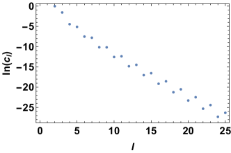
Figure 1: Monopole harmonic expansion coefficients for $\chi=2$ orbital-triplet pairing. Log of the coefficients in the expansion $\Delta^{triplet}_{proj,\chi=2}\propto\sum_{l=2}^{\infty}c_{l}\left[Y_{-2,l,-2}(\theta_{p},\phi_{p})+(-1)^{l}Y_{-2,l,2}(\theta_{p},\phi_{p})\right]$.

For the $\chi=2$ case, the BdG nodes for orbital-singlet and orbital-triplet pairing differ in more than just location. In particular, the orbital-triplet projected gap function vanishes at four points along the equator, $\theta_{p}=\pi/2$ and $\phi_{p}=0,\pm\frac{\pi}{2},\pi$, while the orbital-singlet projected gap function vanishes only at the two poles, $\theta_{p}=0,\pi$. Expanding about the nodes of the projected gap function, ${\bf p}=\pm\mu\hat{p}_{z}+\delta{\bf p}$ for orbital-singlet pairing and ${\bf p}=\pm\mu\hat{p}_{x}+\delta{\bf p}$ and ${\bf p}=\pm\mu\hat{p}_{y}+\delta{\bf p}$ for orbital-triplet pairing, the effective Hamiltonians of the BdG nodes are

$$\mathcal{H}^{singlet}_{proj,\chi=2}(\pm\mu\hat{p}_{z},\delta{\bf p}) =\pm\delta p_{z}\sigma_{z}+\frac{\Delta_{0}}{\mu^{2}}(\delta p_{x}^{2}-\delta p_{y}^{2})\sigma_{x}$$ (16)

$$\hskip 11.38092pt\pm\frac{\Delta_{0}}{\mu^{2}}2\delta p_{x}\delta p_{y}\sigma_{y}$$

$$\mathcal{H}^{triplet}_{proj,\chi=2}(\pm\mu\hat{p}_{x},\delta{\bf p}) =\pm\delta p_{x}\sigma_{z}-\frac{\Delta_{0}}{\mu}\sqrt{2}\delta p_{z}\sigma_{x}$$

$$\hskip 11.38092pt\pm\frac{\Delta_{0}}{\mu}2\delta p_{y}\sigma_{y}$$

$$\mathcal{H}^{triplet}_{proj,\chi=2}(\pm\mu\hat{p}_{y},\delta{\bf p}) =\pm\delta p_{y}\sigma_{z}-\frac{\Delta_{0}}{\mu}\sqrt{2}\delta p_{z}\sigma_{x}$$

$$\hskip 11.38092pt\mp\frac{\Delta_{0}}{\mu}2\delta p_{x}\sigma_{y}.$$

Thus, we find that the orbital-singlet pairing leads to two quadratic BdG nodes, while the orbital-triplet pairing leads to four linear BdG nodes.

III ${\bf k}\cdot{\bf p}$ Models of Cd₃As₂

III.1 Symmetry analysis for Dirac semimetal Cd₃As₂

We review the form of the ${\bf k}\cdot{\bf p}$ Hamiltonian for the Dirac semimetal Cd₃As₂ [4]. The $D_{4h}$ point group together with time reversal symmetry of the material in the absence of magnetic dopants restricts the structure of the ${\bf k}\cdot{\bf p}$ Hamiltonian [5]. Following the theory of invariants [6], the symmetry condition $D(g)\mathcal{H}(g^{-1}{\bf k})D(g)^{-1}=\mathcal{H}({\bf k})$ implies that for a particular basis of matrices, the Hamiltonian matrix is a sum of matrices paired with functions of ${\bf k}$ that both belong to the same irreducible representation of $D_{4h}$.

As discussed in Ref. [4], the bands relevant to the Dirac crossing constitute the spin-orbit coupled basis $(|s_{1/2},\frac{1}{2}\rangle,|p_{3/2},\frac{3}{2}\rangle,|s_{1/2},-\frac{1}{2}\rangle,|p_{3/2},-\frac{3}{2}\rangle)^{T}$. The symmetry group is generated by time reversal $\Theta$, inversion $\Pi$, rotation $C_{4}$ about the $z$ axis, and rotation $C_{2}^{\prime}$ about the $x$ axis, which in the spin-orbit coupled basis can be written as

$$D(\Theta) =i\sigma_{y}\otimes I\mathcal{K}$$ (17)

$$D(\Pi) =I\otimes\tau_{z}$$

$$D(C_{4}) =e^{-i\frac{\pi}{4}\Sigma}\equiv e^{-i\frac{\pi}{4}\sigma_{z}\otimes(2I-\tau_{z})}$$

$$D(C_{2}^{\prime}) =-i\sigma_{x}\otimes\tau_{z},$$

with the $\tau_{i}$ Pauli matrices acting on the orbital part of the basis (s/p) and $\sigma_{i}$ acting on the spin part, with spin $\uparrow/\downarrow$ corresponding to $\mathrm{sgn}(J_{z})=\pm$. Here $\mathcal{K}$ is the complex conjugation operator. The full double group need not be considered since $2\pi$ spin rotation acts as $-I\otimes I$ and thus commutes with $\mathcal{H}({\bf k})$. The presence of both time reversal and parity requires that the gamma matrices appearing in $\mathcal{H}({\bf k})$ be even under the product operation $\Theta\Pi$, since ${\bf k}$ is even under this combined symmetry. This restricts the basis of allowed matrices to $\Gamma_{i}$ for $i=0,\dots,5$ with $\Gamma_{0}$ the identity, $\Gamma_{1,2,3}=\sigma_{x,y,z}\otimes\tau_{x}$, and $\Gamma_{4,5}=I\otimes\tau_{y,z}$.

The characters of $\Gamma_{i}$ under the symmetry transformations $D(\Theta),D(\Pi),$ or $D(C_{2}^{\prime})$ are listed in Table 1. $\Gamma_{1},\Gamma_{2},$ and $\Gamma_{5}$ form one-dimensional representations while $(\Gamma_{3},\Gamma_{4})$ is an irreducible two-dimensional representation, since $C_{2}^{\prime}$ and $C_{4}$ respectively act as $\sigma_{z}$ and $-i\sigma_{y}$ on $(\Gamma_{3},\Gamma_{4})$ and thus cannot be simultaneously diagonalized. As a result, comparison to the character table [7] for $D_{4h}$ uniquely identifies the corresponding irreducible representations, listed in Table 1 along with the corresponding basis functions to lowest nonzero order in ${\bf k}$.

$\Gamma_{i}$	$\Theta$	$\Pi$	$C_{2}^{\prime}$	$C_{4}$	Rep	Functions
$\Gamma_{0}=I\otimes I$	$1$	$1$	$1$	$1$	$A_{1g}$	$k_{x}^{2}+k_{y}^{2},k_{z}^{2}$
$\Gamma_{1}=\sigma_{x}\otimes\tau_{x}$	$-1$	$-1$	$-1$	$-1$	$B_{2u}$	$k_{z}(k_{x}^{2}-k_{y}^{2})$
$\Gamma_{2}=\sigma_{y}\otimes\tau_{x}$	$-1$	$-1$	$1$	$-1$	$B_{1u}$	$k_{x}k_{y}k_{z}$
$\Gamma_{3}=\sigma_{z}\otimes\tau_{x}$
$\Gamma_{4}=I\otimes\tau_{y}$	$-2$	$-2$	$0$	$0$	$E_{u}$	$(k_{x},k_{y})$
$\Gamma_{5}=I\otimes\tau_{z}$	$1$	$1$	$1$	$1$	$A_{1g}$	$k_{x}^{2}+k_{y}^{2},k_{z}^{2}$

Table 1: Transformation of $\Gamma_{i}$ under the $D_{4h}$ symmetries. Comparison to a $D_{4h}$ character table allows the irreducible representations and corresponding basis functions to be identified.

The symmetry-allowed $\mathcal{H}({\bf k})$ is then

$$\mathcal{H}({\bf k})= \left(e_{0}+e_{1}k_{z}^{2}+e_{2}(k_{x}^{2}+k_{y}^{2})\right)\Gamma_{0}$$ (18)

$$+\left(M_{0}+M_{1}k_{z}^{2}+M_{2}(k_{x}^{2}+k_{y}^{2})\right)\Gamma_{5}$$

$$+A(k_{x}\Gamma_{3}-k_{y}\Gamma_{4})$$

$$+B_{1}k_{z}(k_{x}^{2}-k_{y}^{2})\Gamma_{1}+B_{2}2k_{z}k_{x}k_{y}\Gamma_{2},$$

with all coefficients real due to time reversal symmetry and the factor of $2$ on the $B_{2}$ term added for convenience. The appropriate basis vector in the two-dimensional $E_{u}$ subspace is selected by requiring $D(g)H(g^{-1}{\bf k})D(g)^{-1}=H({\bf k})$. The off-diagonal terms in Eq. (18) are

$$\mathcal{H}_{A,B}({\bf k})=\begin{pmatrix}0&Ak_{+}&0&f_{B}({\bf k})\\ Ak_{-}&0&f_{B}({\bf k})&0\\ 0&f_{B}^{*}({\bf k})&0&-Ak_{-}\\ f_{B}^{*}({\bf k})&0&-Ak_{+}&0\end{pmatrix}$$ (19)

with $f_{B}({\bf k})\equiv Gk_{z}k_{-}^{2}+G^{\prime}k_{z}k_{+}^{2}$ and $G,G^{\prime}=\frac{B_{1}\pm B_{2}}{2}$ for $k_{\pm}=k_{x}\pm ik_{y}$. In particular, $f_{B}({\bf k})$ includes only the $k_{-}^{2}$ term when $B_{1}=B_{2}$, which is not generally required by the $D_{4h}$ symmetry.

As noted in Ref. [8], the $G^{\prime}$ term arises due to weak crystal field effects and can be taken to be zero. In fact, the inclusion of a small $G^{\prime}<G$ does not affect topological properties of the magnetically doped model, such as the Chern number and hence the number of BdG nodes required by the topological pairing, as the chiralities of the $\chi=\pm 2$ Weyl nodes change only when $G^{\prime}=G$.

III.2 ${\bf k}\cdot{\bf p}$ parameters for magnetically doped Cd₃As₂

In the presence of magnetic dopants, modeled by a Zeeman field in the $\hat{k}_{z}$ direction, the Weyl points near $k_{z}=k_{D}$, the location of the Dirac node in the absence of magnetic dopants, are described by

$${\cal{H}}({\bf k})=(\epsilon_{D}-\mu)I+\begin{pmatrix}v_{s}\tilde{k}_{z}+\beta_{s}h&Ak_{+}&0&Gk_{-}^{2}\\ Ak_{-}&-v_{p}\tilde{k}_{z}+\beta_{p}h&Gk_{-}^{2}&0\\ 0&Gk_{+}^{2}&v_{s}\tilde{k}_{z}-\beta_{s}h&-Ak_{-}\\ Gk_{+}^{2}&0&-Ak_{+}&-v_{p}\tilde{k}_{z}-\beta_{p}h\end{pmatrix},$$ (20)

as studied in Ref. [8], with fit parameters reproduced in Table 2 for convenience.

$v_{s}$(eV $\mathring{A}$)	$v_{p}$(eV $\mathring{A}$)	$A$ (eV $\mathring{A}$)	$G$ (eV $\mathring{A}^{2}$)
$2.68$	$0.56$	$0.99$	$10$
$\beta_{s}$ (eV/T)	$\beta_{p}$ (eV/T)	$h$ (T)	$k_{D}$ ($\mathring{A}^{-1}$)
$5.4\times 10^{-5}$	$1.15\times 10^{-4}$	$100$	$0.037$

Table 2: Parameters in the ${\bf k}\cdot{\bf p}$ Hamiltonian Eq. (20), as calculated in Ref. [8].

IV Model of magnetically doped Cd₃As₂ with $\beta_{p}=\beta_{s}$

We consider a deformation of the model in Eq. (20) with $\beta_{p}=\beta_{s}=5.4\times 10^{-5}eV/T$. This simplification allows the eigenstates to be written in a simpler form where the appropriate gauges for smooth eigenstates near the poles of each Fermi pocket be can be easily identified. This model is a continuous deformation of Eq. (20) that preserves the topological structure of the Fermi pockets.

The Hamiltonian matrix kernel for $k_{z}>0$ can be written as

$$\mathcal{H}_{+}({\bf k}) =\left[v_{-}(k_{z}-k_{D})-\mu\right]I+\beta_{-}h\sigma_{z}\otimes\tau_{z}+\beta_{+}h\sigma_{z}\otimes I$$ (21)

$$+v_{+}(k_{z}-k_{D})I\otimes\tau_{z}-Ak_{y}I\otimes\tau_{y}+Ak_{x}\sigma_{z}\otimes\tau_{x}$$

$$+G(k_{x}^{2}-k_{y}^{2})\sigma_{x}\otimes\tau_{x}+G2k_{x}k_{y}\sigma_{y}\otimes\tau_{x}$$

$$\equiv f_{0}(k_{z})I+B\Gamma_{12}+\beta_{-}h\Gamma_{34}+\sum_{i=1}^{5}d_{i}\Gamma_{i}$$

where $v_{\pm}=\frac{v_{s}\pm v_{p}}{2}$, $\beta_{\pm}=\frac{\beta_{s}\pm\beta_{p}}{2}$, and $B=\beta_{+}h$. With $\beta_{s}\neq\beta_{p}$, this model is exactly the ${\bf k}\cdot{\bf p}$ model in Eq. (20), here labeled $\mathcal{H}_{+}$ to emphasize that this linearized model is valid for $k_{z}>0$. The five anticommuting gamma matrices are $\Gamma_{1,2,3}=\sigma_{x,y,z}\otimes\tau_{x}$ and $\Gamma_{4,5}=I\otimes\tau_{y,z}$, as in Sec. III.1, and we denote products of gamma matrices by $\Gamma_{nm}\equiv-i\Gamma_{n}\Gamma_{m}$. Thus, $f_{0}(k_{z})=v_{-}(k_{z}-k_{D})-\mu$, $d_{1}=G(k_{x}^{2}-k_{y}^{2})$, $d_{2}=G2k_{x}k_{y}$, $d_{3}=Ak_{x}$, $d_{4}=-Ak_{y}$, and $d_{5}=v_{+}(k_{z}-k_{D})$. For the simplified model with $\beta_{p}=\beta_{s}$, the model inovlves only six gamma matrices, as $\beta_{-}=0$. With $\beta_{-}=0$, the energies are

$$E_{s_{1},s_{2}}=f_{0}(k_{z})+s_{1}\sqrt{B^{2}+d^{2}+s_{2}2Bd^{(3)}},$$ (22)

labeled by the signs $s_{1},s_{2}=\pm 1$, and with $d^{(3)}\equiv\sqrt{d_{3}^{2}+d_{4}^{2}+d_{5}^{2}}$.

For $k_{z}<0$, the parity-related Hamiltonian is $\mathcal{H}_{-}({\bf k})=\Pi\mathcal{H}_{+}(-{\bf k})\Pi$, with $\Pi=\Gamma_{5}=I\otimes\tau_{z}$. In other words, we consider the model in Eq. (20) with $\beta_{p}=\beta_{s}$ and extended to all ${\bf k}$ by requiring parity symmetry,

$$\mathcal{H}({\bf k})=\begin{cases}\mathcal{H}_{+}({\bf k})&k_{z}>0\\ \mathcal{H}_{-}({\bf k})=\Pi\mathcal{H}_{+}(-{\bf k})\Pi&k_{z}<0.\end{cases}$$ (23)

The BdG Hamiltonian, for $k_{z}>0$, is thus

$$\mathcal{H}_{BdG}({\bf k})=\begin{pmatrix}\mathcal{H}({\bf k})&\hat{\Delta}({\bf k})\\ \hat{\Delta}({\bf k})^{\dagger}&-\mathcal{H}^{*}(-{\bf k})\end{pmatrix}=\begin{pmatrix}\mathcal{H}_{+}({\bf k})&\hat{\Delta}({\bf k})\\ \hat{\Delta}({\bf k})^{\dagger}&-\Pi\mathcal{H}_{+}^{*}({\bf k})\Pi\end{pmatrix},$$ (24)

where, in terms of $d_{i}$, the hole block is

$$\mathcal{H}_{h}({\bf k})\equiv-\Pi\mathcal{H}_{+}^{*}({\bf k})\Pi= -f_{0}(k_{z})-B\Gamma_{12}$$ (25)

$$+(d_{1},-d_{2},d_{3},-d_{4},-d_{5})\cdot\mathbf{\Gamma}.$$

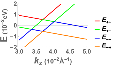
Figure 2: Spectrum along the $k_{z}$ axis for $\beta_{p}=\beta_{s}$.

The eigenvectors of Eq. (21) are, up to an overall phase choice,

$$|\psi_{s_{1},s_{2}}\rangle =\frac{1}{\mathcal{N}}\begin{pmatrix}s_{2}\frac{(d_{1}-id_{2})}{d_{12}}d_{34}g^{(3)}_{s_{1},s_{2}}\\ \frac{i(d_{4}-id_{3})(d_{1}-id_{2})}{d_{34}d_{12}}\left[d_{34}^{2}+(d^{(3)}-s_{2}d_{5})g_{5,s_{1},s_{2}}\right]\\ s_{2}\frac{i(d_{4}-id_{3})}{d_{34}}d_{12}(d^{(3)}-s_{2}d_{5})\\ d_{34}d_{12}\end{pmatrix},$$ (26)

$$N =\sqrt{\left(d_{34}g^{(3)}_{s_{1},s_{2}}\right)^{2}+\left(d_{34}^{2}+(d^{(3)}-s_{2}d_{5})g_{5,s_{1},s_{2}}\right)^{2}+\left(d_{12}(d^{(3)}-s_{2}d_{5})\right)^{2}+d_{34}^{2}d_{12}^{2}}$$

with $s_{1},s_{2}=\pm 1$, $d_{ij}=\sqrt{d_{i}^{2}+d_{j}^{2}}$, $g^{(3)}_{s_{1},s_{2}}=s_{2}B+d^{(3)}+s_{1}s_{2}\sqrt{B^{2}+d^{2}+s_{2}2Bd^{(3)}}$, and $g_{5,s_{1},s_{2}}=g^{(3)}_{s_{1},s_{2}}-d^{(3)}-s_{2}d_{5}$. The spectrum along the $k_{z}$ axis is shown near $k_{D}$ in Fig. 2. There are four Weyl nodes at $k_{z}^{w_{1}}=k_{D}$, $k_{z}^{w_{2}}=k_{D}-B/v_{+}$, $k_{z}^{w_{3}}=k_{D}+B/v_{+}$, $k_{z}^{w_{4}}=k_{D}$ with energies $E_{w_{1}}=-B$, $E_{w_{2}}=-Bv_{-}/v_{+}$, $E_{w_{3}}=Bv_{-}/v_{+}$, $E_{w_{4}}=B$.

For a Fermi pocket defined by $E_{s_{1},s_{2}}=0$, the pocket is described by the eigenstate $|\psi_{s_{1},s_{2}}\rangle$ of $\mathcal{H}({\bf k})$. The Fermi surface projection selects the zero-energy eigenstates of $\mathcal{H}({\bf k})$ and $\mathcal{H}_{h}({\bf k})$, the latter of which has eigenstates

$$|\psi^{h}_{-s_{1},s_{2}}\rangle=-\Pi\mathcal{K}|\psi_{s_{1},s_{2}}\rangle,$$ (27)

where $\mathcal{K}$ is the complex conjugation operator, at energy $E^{h}_{-s_{1},s_{2}}=-E_{s_{1},s_{2}}=0$. The overall phase in Eq. (27) is chosen for convenience to keep the final component of the state positive. The projected gap function over the $E_{s_{1},s_{2}}=0$ Fermi pocket to lowest order is then

$$\Delta_{proj}({\bf k})=\langle\psi_{s_{1},s_{2}}|\hat{\Delta}({\bf k})|\psi^{h}_{-s_{1},s_{2}}\rangle=-\langle\psi_{s_{1},s_{2}}|\hat{\Delta}({\bf k})\Pi\mathcal{K}|\psi_{s_{1},s_{2}}\rangle.$$ (28)

The phase winding in Eq. (26) requires the eigenvectors to be written with different overall phase winding near different Fermi surface points on the $k_{z}$ axis to avoid phase winding singularities in nonzero components of the eigenvector. For the Fermi pockets with $k_{z}>0$, the nontrivial Fermi pockets, the pockets cross the $k_{z}$ axis twice and we refer to the point on the $k_{z}$ axis furthest from the $\Gamma$ point (${\bf k}=0$) as the north pole and the point on the $k_{z}$ axis closest to the $\Gamma$ point as the south pole. With two such pockets, we call the pocket with south pole closest to $\Gamma$ $FS_{1}$ and the other pocket $FS_{2}$, and the north and south pole locations are listed in Table 3. The Fermi pockets at $k_{z}<0$ are related by parity. When $\mu>\mu_{U,1}\equiv k_{D}v_{p}-B$ or $\mu<\mu_{L,1}\equiv-(k_{D}v_{s}-B)$, $FS_{1}$ has merged with the parity-related pocket and is trivial. For $\mu>\mu_{U,2}\equiv k_{D}v_{p}+B$ or $\mu<\mu_{L,2}\equiv-(k_{D}v_{s}+B)$, there are only two Fermi pockets in the entire Brillouin zone, and both are trivial. The eigenvectors in Eq. (26) can only have phase winding singularities along the $k_{z}$ axis and can be smoothly defined on any Fermi pocket using at most two patches. The eigenvectors at each Fermi pocket are shown in Table 4 in the appropriate smooth gauge at each pole. As in Sec. I.1, the transition function, and hence the Chern number, can be read from the gauge at each pole together with knowledge of whether the Fermi pocket is electron- or hole-type. For example at $\mu_{U,1}>\mu>B$, the smaller Fermi pocket, $FS_{2}$, is electron type and has $|\psi^{N}_{++}\rangle=e^{-i\phi_{\bf k}}|\psi^{S}_{++}\rangle$, indicating a transition function with $q=1/2$ in Eq. (1) and hence Chern number $C=+1$. For the hole pocket $FS_{2}$ at $B\frac{v_{-}}{v_{+}}>\mu>-B\frac{v_{-}}{v_{+}}$, the appropriate gauges satisfy $|\psi_{--}^{N}\rangle=e^{2i\phi_{\bf k}}|\psi_{--}^{S}\rangle$, which, due to the hole pocket reversing the normal direction, corresponds to $C=+2$.

$\mu$	$k_{z,1}^{S}$	$k_{z,1}^{N}$	$k_{z,2}^{S}$	$k_{z,2}^{N}$
$-B>\mu>\mu_{L,1}$	$k_{D}-\frac{B-\mu}{v_{s}}$	$k_{D}+\frac{B-\mu}{v_{p}}$	$k_{D}+\frac{B+\mu}{v_{s}}$	$k_{D}-\frac{B+\mu}{v_{p}}$
$-B\frac{v_{-}}{v_{+}}>\mu>-B$	$k_{D}-\frac{B-\mu}{v_{s}}$	$k_{D}+\frac{B-\mu}{v_{p}}$	$k_{D}-\frac{B+\mu}{v_{p}}$	$k_{D}+\frac{B+\mu}{v_{s}}$
$B\frac{v_{-}}{v_{+}}>\mu>-B\frac{v_{-}}{v_{+}}$	$k_{D}-\frac{B+\mu}{v_{p}}$	$k_{D}-\frac{B-\mu}{v_{s}}$	$k_{D}+\frac{B+\mu}{v_{s}}$	$k_{D}+\frac{B-\mu}{v_{p}}$
$B>\mu>B\frac{v_{-}}{v_{+}}$	$k_{D}-\frac{B+\mu}{v_{p}}$	$k_{D}+\frac{B+\mu}{v_{s}}$	$k_{D}-\frac{B-\mu}{v_{s}}$	$k_{D}+\frac{B-\mu}{v_{p}}$
$\mu_{U,1}>\mu>B$	$k_{D}-\frac{\mu+B}{v_{p}}$	$k_{D}+\frac{\mu+B}{v_{s}}$	$k_{D}-\frac{\mu-B}{v_{p}}$	$k_{D}+\frac{\mu-B}{v_{s}}$

Table 3: $k_{z}$ coordinates for the nodes of the two $k_{z}>0$ Fermi pockets for $\mu_{U,1}>\mu>\mu_{L,1}$. For larger or smaller $\mu$, $FS_{1}$ has the north pole $k_{z,1}^{N}$ given respectively in the first or last row with the remaining pole at $-k_{z,1}^{N}$. For $\mu>\mu_{U,2}$ or $\mu<\mu_{L,2}$, the poles of $FS_{2}$ are similarly at $\pm k_{z,2}^{N}$.

$\mu$	$FS_{1}$ $S$ pole state	$FS_{1}$ $N$ pole state	$FS_{2}$ $S$ pole state	$FS_{2}$ $N$ pole state
$-B>\mu>\mu_{L,1}$	$e^{2i\phi_{\bf k}}|\psi_{--}\rangle$	$e^{3i\phi_{\bf k}}|\psi_{--}\rangle$	$e^{i\phi_{\bf k}}|\psi_{-+}\rangle$	$|\psi_{-+}\rangle$
$-B\frac{v_{-}}{v_{+}}>\mu>-B$	$e^{2i\phi_{\bf k}}|\psi_{--}\rangle$	$e^{3i\phi_{\bf k}}|\psi_{--}\rangle$	$|\psi_{--}\rangle$	$e^{i\phi_{\bf k}}|\psi_{--}\rangle$
$B\frac{v_{-}}{v_{+}}>\mu>-B\frac{v_{-}}{v_{+}}$	$|\psi_{+-}\rangle$	$e^{2i\phi_{\bf k}}|\psi_{+-}\rangle$	$e^{i\phi_{\bf k}}|\psi_{--}\rangle$	$e^{3i\phi_{\bf k}}|\psi_{--}\rangle$
$B>\mu>B\frac{v_{-}}{v_{+}}$	$|\psi_{+-}\rangle$	$e^{i\phi_{\bf k}}|\psi_{+-}\rangle$	$e^{2i\phi_{\bf k}}|\psi_{+-}\rangle$	$e^{3i\phi_{\bf k}}|\psi_{+-}\rangle$
$\mu_{U,1}>\mu>B$	$|\psi_{+-}\rangle$	$e^{i\phi_{\bf k}}|\psi_{+-}\rangle$	$e^{3i\phi_{\bf k}}|\psi_{++}\rangle$	$e^{2i\phi_{\bf k}}|\psi_{++}\rangle$

Table 4: States describing the two $k_{z}>0$ Fermi pockets for $\mu_{U,1}>\mu>\mu_{L,1}$ in the appropriate smooth gauge at each pole.

V Gap function representations

The possible proximitized gap functions in irreducible representations of the $C_{4h}$ point group symmetry of the magnetically doped model in Eq. (20) can be constructed from products of momentum and matrix irreps in the spin-orbital basis. The representation of the symmetry group acting on the $4\times 4$ spin-orbital basis is generated by $D(i)=I_{2\times 2}\otimes\tau_{z}$ and $D(C_{4})=e^{-i\frac{\pi}{4}[\sigma_{z}\otimes(2I_{2\times 2}-\tau_{z})]}=\text{diag}[e^{\frac{-i\pi}{4}},e^{\frac{-i3\pi}{4}},e^{\frac{i\pi}{4}},e^{\frac{i3\pi}{4}}]$. Since $C_{4h}$ is abelian, the irreps are one-dimensional, and each matrix $M$ that is in an irrep satisfies $D(g)MD(g)^{T}=\chi(g)M$ for each group element $g$. Note that the transpose $D(g)^{T}$ is used rather than the conjugate transpose since the gap function mixes particle and hole blocks of the BdG matrix. In terms of $M_{ij}\equiv\sigma_{i}\otimes\tau_{j}$, with $0,1,2,3$ labeling the identity matrix and $x,y,$ and $z$ Pauli matrices, the sixteen matrices in Table 5a span the space of $4\times 4$ matrices and are irreps of $C_{4h}$. The irreps are given both labels used in the Bilbao Crystallographic Server point group table for $C_{4h}$, reproduced in Table 5b for convenience [9].

Irrep	Matrices
$A_{g}(\Gamma_{1}^{+})$	$M_{10}$, $M_{13}$, $M_{20}$, $M_{23}$
$\-{}^{1}E_{g}(\Gamma_{4}^{+})$	$M_{00}+M_{33}$, $M_{03}+M_{30}$
$\-{}^{2}E_{g}(\Gamma_{3}^{+})$	$M_{00}-M_{33}$, $M_{03}-M_{30}$
$B_{u}(\Gamma_{2}^{-})$	$M_{01}$, $M_{02}$, $M_{31}$, $M_{32}$
$\-{}^{1}E_{u}(\Gamma_{4}^{-})$	$M_{11}+M_{22}$, $M_{12}-M_{21}$
$\-{}^{2}E_{u}(\Gamma_{3}^{-})$	$M_{11}-M_{22}$, $M_{12}+M_{21}$

(a) Gap function matrix irreps.

Irreps	$E$	$\Pi$	$C_{4}$	Basis Functions
$A_{g}(\Gamma_{1}^{+})$	$1$	$1$	$1$	$k_{z}^{2}$, $k_{x}^{2}+k_{y}^{2}$
$B_{g}(\Gamma_{2}^{+})$	$1$	$1$	$-1$	$k_{x}k_{y}$, $k_{x}^{2}-k_{y}^{2}$
$\-{}^{2}E_{g}(\Gamma_{3}^{+})$	$1$	$1$	$i$	$k_{z}(k_{x}+ik_{y})$
$\-{}^{1}E_{g}(\Gamma_{4}^{+})$	$1$	$1$	$-i$	$k_{z}(k_{x}-ik_{y})$
$A_{u}(\Gamma_{1}^{-})$	$1$	$-1$	$1$	$k_{z}$
$B_{u}(\Gamma_{2}^{-})$	$1$	$-1$	$-1$	$k_{z}k_{x}k_{y}$, $k_{z}(k_{x}^{2}-k_{y}^{2})$
$\-{}^{2}E_{u}(\Gamma_{3}^{-})$	$1$	$-1$	$i$	$k_{x}+ik_{y}$
$\-{}^{1}E_{u}(\Gamma_{4}^{-})$	$1$	$-1$	$-i$	$k_{x}-ik_{y}$

(b) $C_{4h}$ character table.

Table 5: Irrep tables listing (a) the gap function matrices in each irreducible representation of $C_{4h}$ under the transformation $D(g)MD(g)^{T}$ and (b) the character table for $C_{4h}$. In (a), The matrices are expressed as tensor products of Pauli matrices, $M_{ij}=\sigma_{i}\otimes\tau_{j}$. The character table in (b) includes the characters for the identity $E$ and group generators, parity $\Pi$ and $\pi/2$ clockwise rotation about the $z$ axis $C_{4}$.

For any matrix part, the momentum irrep must be chosen so that the condition required by Fermi statistics, $\Delta_{\alpha\beta}({\bf k})=-\Delta_{\beta\alpha}(-{\bf k})$, is satisfied. Further, the projected gap function vanishes for proximitized gap functions with matrix part $M_{01}$, $M_{10}$, $M_{11}\pm M_{22}$, $M_{20}$, $M_{23}$, or $M_{31}$. Note that the projected gap function to lowest order is calculated from $\Delta_{proj}({\bf k})=\langle\psi_{s_{1},s_{2}}|\hat{\Delta}({\bf k})|\psi^{h}_{-s_{1},s_{2}}\rangle=\langle\psi_{s_{1},s_{2}}|\hat{\Delta}({\bf k})(-\Pi)\mathcal{K}|\psi_{s_{1},s_{2}}\rangle$, with $\Pi=M_{03}$ the parity operator and $\mathcal{K}$ the complex conjugation operator. The projected gap function to lowest order is thus of the form $v^{T}Mv$ and vanishes when the matrix $M=-\hat{\Delta}({\bf k})\Pi$ is antisymmetric, $M=-M^{T}$, as is the case for $\hat{\Delta}({\bf k})\propto M_{01},M_{11}\pm M_{22},M_{20},M_{23}$ and $M_{31}$. These gap functions thus vanish as a result of parity symmetry. The final vanishing gap function, $\hat{\Delta}({\bf k})\propto M_{10}$, is a special case for the $\beta_{p}=\beta_{s}$ model that vanishes since $\psi_{s1,s2}^{(1)}\psi_{s1,s2}^{(3)}-\psi_{s1,s2}^{(2)}\psi_{s1,s2}^{(4)}=0$, where $\psi_{s1,s2}^{(j)}$ is the $j$th component of $|\psi_{s1,s2}\rangle$ in the spin-orbital basis. In the full model, Eq. (20) with $\beta_{p}\neq\beta_{s}$, we expect a proximitized gap function with matrix $M_{10}$ to have qualitatively similar projected gap function structure to one with $M_{13}$, both of which are in the $A_{g}(\Gamma_{1}^{+})$ representation.

Accounting for Fermi statistics, the pairings $\hat{\Delta}({\bf k})$ that lead to nonvanishing projected gap functions can be in one of four irreps, $A_{u},B_{u},\-^{2}E_{u},$ and $\-{}^{1}E_{u}$. In the following tables, the phase winding patterns are shown for the nine $M_{ij}$ matrices leading to nonvanishing projected gap functions in the $\beta_{p}=\beta_{s}$ model. For simplicity, only momentum-independent pairings and pairings with $k_{z}/k_{D}$ momentum dependence are considered. Considering different momentum dependence amounts to simply multiplying by a different function of momentum. The tables include descriptions of the nodes and phase winding from which the vorticity can be read. For rows with multiple pairing matrices listed, the pattern is plotted for the first pairing matrix listed, and the patterns for the rest are qualitatively similar with any differences noted in the description. The projected gap function dispersion near the $k_{z}$-axis nodes is written in terms of $k_{\parallel}=\sqrt{k_{x}^{2}+k_{y}^{2}}$.

Table 6 lists phase winding patterns for the smaller, topologically trivial electron pocket at $\mu=35$meV, which is described by the $|\psi_{++}\rangle$ state in Eq. (26). As this pocket is topologically trivial, $C=0$, the total vorticity vanishes for all pairings. Table LABEL:tab:mu002 lists phase winding patterns for the $C=1$ electron pocket at $k_{z}>0$ for $\mu=20$meV, described by the $|\psi_{++}\rangle$ state. Table LABEL:tab:mu0 lists phase winding patterns for the $C=2$ hole pocket at $k_{z}>0$ for $\mu=0$meV, described by the $|\psi_{--}\rangle$ state. The total vorticity in all cases can be seen to be $2C$. Importantly, the vorticity should be read from the counterclockwise phase winding number with respect to the local normal direction, which points out of the surface shown for electron pockets and into the surface for hole pockets.

V.1 Trivial Fermi Pocket

Proximitized Pairing	Irrep	$\Delta_{proj}({\bf k})$ Phase Winding	Node Locations
$\Delta_{0}\frac{k_{z}}{k_{D}}M_{13}$	$A_{u}(\Gamma_{1}^{-})$		$k_{\parallel}^{3}e^{-i\phi}$ nodes on $k_{z}$ axis.
$\Delta_{0}M_{02}$ $\Delta_{0}M_{32}$	$B_{u}(\Gamma_{2}^{-})$		$k_{\parallel}e^{i\phi}$ nodes on $k_{z}$ axis.
$\Delta_{0}(M_{12}+M_{21})$ $\Delta_{0}\frac{k_{z}}{k_{D}}(M_{00}-M_{33})$ $\Delta_{0}\frac{k_{z}}{k_{D}}(M_{03}-M_{30})$	$\-{}^{2}E_{u}(\Gamma_{3}^{-})$		$k_{\parallel}^{2}e^{2i\phi}$ nodes on $k_{z}$ axis.
$\Delta_{0}(M_{12}-M_{21})$	$\-{}^{1}E_{u}(\Gamma_{4}^{-})$		$k_{\parallel}^{4}$ nodes on $k_{z}$ axis.
$\Delta_{0}\frac{k_{z}}{k_{D}}(M_{00}+M_{33})$ $\Delta_{0}\frac{k_{z}}{k_{D}}(M_{03}+M_{30})$	$\-{}^{1}E_{u}(\Gamma_{4}^{-})$		Gapped on $k_{z}$ axis. Gap function only vanishes at $k_{z}=0$.

Table 6: Table of representative phase winding behavior on the smaller $C=0$ Fermi pocket at $\mu=35$meV.

V.2 $C=1$ Fermi Pocket

Table 7: Table of phase winding behavior for the $C=1$ pocket at $\mu=20$meV.

Proximitized Pairing	Irrep	$\Delta_{proj}^{N}({\bf k})$ Phase Winding (North View)	$\Delta_{proj}^{S}({\bf k})$ Phase Winding (South View)	Node Locations
$\Delta_{0}\frac{k_{z}}{k_{D}}M_{13}$	$A_{u}(\Gamma_{1}^{-})$			$k_{\parallel}^{3}e^{-i\phi}$ gap function node at $N$, $k_{\parallel}^{3}e^{-3i\phi}$ gap function node at $S$.
$\Delta_{0}M_{02}$ $\Delta_{0}M_{32}$	$B_{u}(\Gamma_{2}^{-})$			$k_{\parallel}e^{i\phi}$ gap function node at $N$, $k_{\parallel}e^{-i\phi}$ gap function node at $S$.
$\Delta_{0}(M_{12}+M_{21})$	$\-{}^{2}E_{u}(\Gamma_{3}^{-})$			$k_{\parallel}^{2}e^{-2i\phi}$ gap function node at $N$, $k_{\parallel}^{4}e^{-4i\phi}$ gap function node at $S$.
$\Delta_{0}\frac{k_{z}}{k_{D}}(M_{00}-M_{33})$ $\Delta_{0}\frac{k_{z}}{k_{D}}(M_{03}-M_{30})$	$\-{}^{2}E_{u}(\Gamma_{3}^{-})$			$k_{\parallel}^{2}e^{2i\phi}$ gap function node at $N$, gapped at $S$.
$\Delta_{0}(M_{12}-M_{21})$	$\-{}^{1}E_{u}(\Gamma_{4}^{-})$			$k_{\parallel}^{4}$ gap function node at $N$, $k_{\parallel}^{2}e^{-2i\phi}$ gap function node at $S$.
$\Delta_{0}\frac{k_{z}}{k_{D}}(M_{00}+M_{33})$ $\Delta_{0}\frac{k_{z}}{k_{D}}(M_{03}+M_{30})$	$\-{}^{1}E_{u}(\Gamma_{4}^{-})$			Gapped at $N$, $k_{\parallel}^{2}e^{-2i\phi}$ gap function node at $S$.

V.3 $C=2$ Fermi Pocket

Table 8: Table of phase winding behavior for the $C=2$ hole pocket at $\mu=0$ meV.

Proximitized Pairing	Irrep	$\Delta_{proj}^{N}({\bf k})$ Phase Winding (North View)	$\Delta_{proj}^{S}({\bf k})$ Phase Winding (South View)	Node Locations
$\Delta_{0}\frac{k_{z}}{k_{D}}M_{13}$	$A_{u}(\Gamma_{1}^{-})$			$k_{\parallel}^{3}e^{-3i\phi}$ gap function node at $N$, $k_{\parallel}^{3}e^{i\phi}$ gap function node at $S$.
$\Delta_{0}M_{02}$ $\Delta_{0}M_{32}$	$B_{u}(\Gamma_{2}^{-})$			$k_{\parallel}e^{-i\phi}$ nodes at N and S poles. Four nodes with $e^{i\phi^{\prime}}$ local winding at $\phi=\pm\pi/4,\pm 3\pi/4$ around concave region near S. For $M_{32}$, these nodes are at $\phi=0,\pm\pi/2,\pi$ instead.
$\Delta_{0}(M_{12}+M_{21})$	$\-{}^{2}E_{u}(\Gamma_{3}^{-})$			$k_{\parallel}^{4}e^{-4i\phi}$ gap function node at $N$, $k_{\parallel}^{4}$ gap function node at $S$.
$\Delta_{0}\frac{k_{z}}{k_{D}}(M_{00}-M_{33})$ $\Delta_{0}\frac{k_{z}}{k_{D}}(M_{03}-M_{30})$	$\-{}^{2}E_{u}(\Gamma_{3}^{-})$			Gapped at N and S. Four nodes with $e^{i\phi^{\prime}}$ local winding at $\phi=0,\pm\pi/2,\pi$ around concave region near S. For $M_{03}-M_{30}$, these nodes are at $\phi=\pm\pi/4,\pm 3\pi/4$ instead.
$\Delta_{0}(M_{12}-M_{21})$	$\-{}^{1}E_{u}(\Gamma_{4}^{-})$			$k_{\parallel}^{2}e^{-2i\phi}$ gap function node at $N$, $k_{\parallel}^{2}e^{2i\phi}$ gap function node at $S$.
$\Delta_{0}\frac{k_{z}}{k_{D}}(M_{00}+M_{33})$ $\Delta_{0}\frac{k_{z}}{k_{D}}(M_{03}+M_{30})$	$\-{}^{1}E_{u}(\Gamma_{4}^{-})$			$k_{\parallel}^{2}e^{-2i\phi}$ nodes at N and S poles. Four nodes with $e^{i\phi^{\prime}}$ local winding at $\phi=0,\pm\pi/2,\pi$ around concave region near S. For $M_{03}-M_{30}$, these nodes are at $\phi=\pm\pi/4,\pm 3\pi/4$ instead.