A Pluto–Charon Sonata IV. Improved Constraints on the Dynamical Behavior and Masses of the Small Satellites

Abstract

We discuss a new set of $\sim$ 500 numerical $n$-body calculations designed to constrain the masses and bulk densities of Styx, Nix, Kerberos, and Hydra. Comparisons of different techniques for deriving the semimajor axis and eccentricity of the four satellites favor methods relying on the theory of Lee & Peale (2006), where satellite orbits are derived in the context of the restricted three body problem (Pluto, Charon, and one massless satellite). In each simulation, we adopt the nominal satellite masses derived in Kenyon & Bromley (2019a), multiply the mass of at least one satellite by a numerical factor $f\geq 1$, and establish whether the system ejects at least one satellite on a time scale $\leq$ 4.5 Gyr. When the total system mass is large ($f\gg 1$), ejections of Kerberos are more common. Systems with lower satellite masses ($f\approx$ 1) usually eject Styx. In these calculations, Styx often ‘signals’ an ejection by moving to higher orbital inclination long before ejection; Kerberos rarely signals in a useful way. The $n$-body results suggest that Styx and Kerberos are more likely to have bulk densities comparable with water ice, $\rho_{SK}\lesssim$ 2 $\rm g~{}cm^{-3}$, than with rock. A strong upper limit on the total system mass, $M_{SNKH}\lesssim 9.5\times 10^{19}$ g, also places robust constraints on the average bulk density of the four satellites, $\rho_{SNKH}\lesssim$ 1.4 $\rm g~{}cm^{-3}$. These limits support models where the satellites grow out of icy material ejected during a major impact on Pluto or Charon.

1 Introduction

In the past two decades, space observations added new insights into the properties of the dwarf planet Pluto. From 2005–2012, HST images revealed four small circumbinary satellites (Weaver et al., 2006; Showalter et al., 2011, 2012). Detailed astrometric analyses of these data demonstrate that the orbits of the central Pluto–Charon binary and the satellites are nearly circular and in a common plane (Buie et al., 2006; Tholen et al., 2008; Brozović et al., 2015; Showalter & Hamilton, 2015). Spectacular observations acquired during the New Horizons flyby confirm that the satellites tumble with approximate rotation periods of 0.43 d to 5.31 d (Showalter & Hamilton, 2015; Weaver et al., 2016). All of the satellites are irregularly shaped and highly reflective. Characteristic radii are $\sim$ 5 km for Styx and Kerberos and $\sim$ 20 km for Nix and Hydra. Albedos are $\sim$ 55% for Kerberos and Nix, 65% for Styx, and 85% for Hydra (Weaver et al., 2016). Although smaller satellites could exist slightly inside the orbit of Styx and outside the orbit of Hydra (Kenyon & Bromley, 2019b), there are no $\gtrsim$ 2 km satellites and a negligible amount of dust between the orbits of Styx and Hydra (Weaver et al., 2016; Lauer et al., 2018).

Deriving limits on the masses and the bulk densities of the small satellites requires detailed $n$-body calculations (e.g., Pires Dos Santos et al., 2011; Youdin et al., 2012; Canup et al., 2021, and references therein). To improve on mass limits inferred from HST observations (Brozović et al., 2015), Kenyon & Bromley (2019a) performed a large suite of $n$-body calculations for various combinations of satellite masses. Within the set of completed simulations, they show that a ‘heavy’ satellite system – where the mass of Kerberos is roughly one third the mass of Hydra and the total system mass is $M_{SNKH}\sim 1.15\times 10^{20}$ g (Brozović et al., 2015) – is unstable on time scales $\lesssim$ 1 Gyr. For a ‘light’ satellite system – where Nix/Hydra have the masses derived by Brozović et al. (2015) and Styx/Kerberos have masses $\sim$ 10–25 times smaller – the analysis yields firm upper limits on the masses of Nix and Hydra. Combined with physical dimensions measured from New Horizons images, the resulting upper limits on the bulk densities are $\rho_{N}\lesssim$ 1.3–1.6 $\rm g~{}cm^{-3}$ for Nix and $\rho_{H}\lesssim$ 1.1–1.5 $\rm g~{}cm^{-3}$ for Hydra. Both upper limits lie below the measured bulk densities for Pluto $\rho_{P}$ = 1.85 $\rm g~{}cm^{-3}$ and Charon $\rho_{C}$ = 1.70 $\rm g~{}cm^{-3}$.

Although the completed simulations in Kenyon & Bromley (2019a) considerably reduced upper limits on the masses of Styx and Kerberos, upper limits on the masses of Nix and Hydra relied on a mixture of completed and unfinished calculations. Using long-term trends in the evolution of a basic ‘geometric’ eccentricity (section 2; see also Sutherland & Kratter, 2019) in many unfinished calculations, Kenyon & Bromley (2019a) placed stronger limits on the masses of Nix and Hydra. While these trends were robust among all the unfinished calculations, periods of a steadily increasing eccentricity might be a temporary feature of a system that fails to eject satellites over the 4.5 Gyr lifetime of the solar system.

Here, we describe a new analysis of a larger set of completed simulations, supplemented with insights gleaned from several ongoing calculations. Adopting nominal (low) masses for Styx and Kerberos, calculations where at least one satellite has been ejected confirm previous upper limits on the masses of Nix and Hydra. Including the small nominal masses of Styx and Kerberos, a more reliable upper limit on the system mass is $M_{SNKH}\lesssim 9.5\times 10^{19}$ g. Coupled with satellite volumes estimated from New Horizons measurements of satellite dimensions, the average bulk density of a satellite $\rho_{SNKH}\lesssim$ 1.4 $\rm g~{}cm^{-3}$.

Another set of completed calculations begins to place limits on the masses of Styx and Kerberos. Analysis of simulations where Styx and Kerberos have bulk densities of 2–3 $\rm g~{}cm^{-3}$ suggest significantly shorter lifetimes than a parallel suite of calculations where the bulk densities are 1.0–1.5 $\rm g~{}cm^{-3}$. Given the robust upper limits on the masses for Nix and Hydra, these results enable approximate upper limits for their bulk densities. While not as stringent as the conclusions for Nix and Hydra, the calculations favor lower bulk densities, $\rho_{SK}\lesssim$ 2 $\rm g~{}cm^{-3}$. This result suggests that these two small satellites are more likely composed of ice than rock, as indicated by their high albedos (Weaver et al., 2016).

Besides improvements in limits on satellite masses, the $n$-body calculations reveal interesting dynamical behavior. In systems with more (less) massive satellites, Kerberos (Styx) is ejected more often than Styx (Kerberos). Ejections of both are very rare. Although Nix is never ejected, Hydra is sometimes ejected when the system mass is large. Among the systems that experience an ejection of Hydra, the frequency of Styx ejections is similar to the frequency of Kerberos ejections. During the period before an ejection, Styx often exhibits an oscillation where growth in its eccentricity is followed by a rise in inclination; increases in inclination are accompanied by a decline in eccentricity. A later rise in eccentricity leads to a prompt ejection. Kerberos almost never follows this type of evolution.

In addition to the analyses described here and in Kenyon & Bromley (2019a), we deposit binary files from all completed $n$-body calculations and some of the programs used to extract and analyze the phase space coordinates at a publicly accessible repository (https://hive.utah.edu/). The combined set of 700 files from Kenyon & Bromley (2019a) and 500 files from this study provides interested researchers a large data set for other analyses.

In the next section, we outline the initial conditions for each calculation and the numerical procedure. We then describe the results and discuss their significance. We conclude with a brief summary.

2 Calculations

2.1 Procedures

We perform numerical calculations with a gravitational $n$-body code which integrates the orbits of Pluto, Charon, and the four smaller satellites in response to their mutual gravitational interactions (e.g., Kenyon & Bromley, 2019b, a, c). The $N$-body code, Orchestra, employs an adaptive sixth-order accurate algorithm based on either Richardson extrapolation (Bromley & Kenyon, 2006) or a symplectic method (Yoshida, 1990; Wisdom & Holman, 1991; Saha & Tremaine, 1992). The code calculates gravitational forces by direct summation and evolves particles accordingly in the center-of-mass frame. The code has passed a stringent set of dynamical tests and benchmarks (Duncan et al., 1998; Bromley & Kenyon, 2006). Bromley & Kenyon (2020) and Kenyon & Bromley (2021) describe recent improvements to the code and cite additional tests of the algorithm.

The calculations do not include tidal or radiation pressure forces on the satellites (e.g., Burns et al., 1979; Hamilton & Burns, 1992; Poppe & Horányi, 2011; Pires dos Santos et al., 2013; Quillen et al., 2017). Radiation pressure forces are significant on dust grains, but satellites with sizes similar to and larger than Styx and Kerberos are unaffected. With a fixed orbit for the central binary, tidal forces have little impact on satellite orbits.

During the symplectic integrations, there is no attempt to resolve collisions between the small satellites or between an ejected satellite and Pluto or Charon. Satellites passing too close to another massive object in the system are eventually ejected. In the adaptive integrator, the code changes the length of timesteps to resolve collisions. In agreement with previous results (Sutherland & Fabrycky, 2016; Smullen et al., 2016; Smullen & Kratter, 2017), small satellites are always ejected from the system and never collide with other small satellites, Charon, or Pluto.

Previous studies demonstrate that the orbits of the small satellites are too far inside the Hill sphere of Pluto to require including the gravity of the Sun or major planets in the integrations (Michaely et al., 2017). For reference, the radius of the Pluto-Charon Hill sphere is $R_{H,PC}\approx 8\times 10^{6}$ km for masses $m_{P}$ = $1.303\times 10^{25}$ g (Pluto) and $m_{C}$ = $1.587\times 10^{24}$ g (Charon). In Hill units, the semimajor axis of Hydra’s orbit, $a_{H}/R_{H,PC}\approx$ 0.008, is well inside the Hill sphere and fairly immune from the gravity of the Sun. For the calculations described in this paper, the $n$-body code follows the orbits of Pluto–Charon and the four small satellites without any contribution from the gravity of the Sun or major planets. Previous tests with the Orchestra code show that including the Sun and the major planets has no impact on satellite orbits (Kenyon & Bromley, 2019a).

Throughout the $n$-body calculations, we record the 6D cartesian phase space variables, the Keplerian semimajor axis $a_{K}$ and eccentricity $e_{K}$, and the orbital inclination $\imath$ at the end of selected time steps. Over total integration times as long as 0.1–2 Gyr, a typical calculation has 30,000 to more than 100,000 of these ‘snapshots’ of the satellite positions, velocities, and Kplerian orbital parameters at machine precision. To avoid unwieldy data sets, we make no attempt to record satellite positions during each orbit. Within the circumbinary environment of Pluto–Charon, satellite orbits precess on time scales ranging from 1.2 yr for Styx to 2.8 yr for Hydra (e.g., Lee & Peale, 2006; Leung & Lee, 2013; Bromley & Kenyon, 2015a). For any calculation, the ensemble of snapshots is insufficient to track the precession of the small satellites.

On the NASA ‘discover’ cluster, 24 hr integrations on a single processor advance the satellite system $\sim$ 4.3 Myr. We perform 28 calculations per node, with each satellite system evolving on one of the 28 cores per node. To derive results for as many sets of initial conditions as possible, the suite of simulations uses 6–10 nodes each day. In this way, each system advances $\sim$ 125 Myr per month.

Table 1: Adopted Masses and Initial Conditions

Satellite	Mass (g)	$x$ (km)	$y$ (km)	$z$ (km)	$v_{x}$ (km s-1)	$v_{y}$ (km s-1)	$v_{z}$ (km s-1)
Pluto	$1.303\times 10^{25}$	-157.8121679944	-456.7988459683	-2071.4067337364	-0.0177032091	-0.0158015359	0.0048362971
Charon	$1.586\times 10^{24}$	1297.1743847853	3752.6022617472	17011.9058384535	0.1453959509	0.1297771902	-0.0397230040
Styx	$6\times 10^{17}$	-30572.8427772584	-26535.8134344897	12311.2908958766	0.0232883189	0.0427977975	0.1464990284
Nix	$4.5\times 10^{19}$	9024.3487802378	15210.7370165008	45591.7573572213	0.1004334400	0.0865524814	-0.0479498746
Kerberos	$9\times 10^{17}$	23564.2070250521	28380.0399507624	44578.0258218278	0.0792537026	0.0630220100	-0.0817084451
Hydra	$4.8\times 10^{19}$	-43331.3261132443	-43628.4575945387	-20506.5419357332	-0.0374001038	-0.0184905611	0.1157937283

2.2 Initial Conditions

All calculations begin with the same measured initial state vector (Brozović et al., 2015) for the 3D cartesian position – $\vec{r}=(x,y,z)$ – and velocity – $\vec{v}=(v_{x},v_{y},v_{z})$ – of each component. Tests with a state vector downloaded from the JPL Horizons website yield indistinguishable results. Kenyon & Bromley (2019a) describe several procedures for deriving the initial state vector for Pluto, which is not included in Brozović et al. (2015). For the satellite masses considered here, we employ the Pluto-2 state vector and the state vectors for the satellites listed in Table 1 (Kenyon & Bromley, 2019a, see also, their Table 2). Test calculations show that outcomes are insensitive to modest changes – 0.5 km in position and 1.0 cm s^-1 in velocity – to the state vectors.

Although all calculations begin with the same initial state vector for Pluto, Charon, and the four small satellites, we perform each simulation with different satellite masses. We first adopt the nominal masses for Styx, $m_{S}$ = 0.6; Nix, $m_{N}$ = 45; Kerberos, $m_{K}$ = 0.9; and Hydra, $m_{H}$ = 48 in units of $10^{18}$ g (Table 1). In some calculations, we multiply the nominal masses for each satellite by a factor $f=n(1+\delta)$, where $n$ is an integer or simple fraction (e.g., 0.5, 0.625, 0.75, 0.875, 1.25 or 1.5) and $\delta$ is a small real number in the range $-$0.01 to 0.01. For a suite of calculations with similar $f$, $n$ and $\delta$ are the same for all satellites. In other simulations, we multiply the mass of a single satellite by a factor $f_{i}$ and set the masses of the remaining satellites at their nominal masses.

To avoid confusion, we use $f$ as a marker for calculations where we multiply the masses of all satellites by a common factor and $f_{i}$ (where $i$ = ‘S’ for Styx, ‘N’ for Nix, ‘K’ for Kerberos, and ‘H’ for Hydra) as markers where 1–2 satellites have masses that differ from the nominal masses. In some calculations, we set $f_{S}=f_{K}$ = 1.5, 2, or 3 and then multiply masses for all four satellites by a common $f$. In these models, Styx and Kerberos have masses $f_{S}\times f$ larger than their nominal masses.

For systems where all satellite masses have the same $f$, the $\delta$ term allows measurement of a range of lifetimes for systems with identical initial positions and velocities and nearly identical masses. In many marginally stable dynamical systems, lifetimes are highly sensitive to initial conditions. Rather than make slight modifications to the adopted state vector to test this sensitivity, we use the $\delta$ term in the expression for $f$. As we showed in Kenyon & Bromley (2019a), 1% variations in $f$ result in factor of 3–10 differences in derived lifetimes.

Before starting the suite of calculations reported here, we considered adopting a volume for each satellite based on New Horizons measurements and deriving system stability as a function of satellite bulk density instead of mass. Although the New Horizons size measurements are nominally more accurate than the HST mass estimates, satellite shapes are not precisely known. For an adopted shape, the $\pm$2 km uncertainty in the dimensions of Nix yields a 40% uncertainty in the volume (Kenyon & Bromley, 2019a). The factor of two larger errors in the dimensions of Hydra place correspondingly weaker constraints on its volume (Weaver et al., 2016).

Within the ensemble of $n$-body calculations, physical collisions are exceedingly rare (see section 2.4 below). Thus, adopted sizes for the satellites have no impact on the outcomes of calculations. System stability depends only on adopted satellite masses. With a precise control of satellite masses within each calculation, we express results in terms of masses instead of bulk densities. Given the uncertainties in shapes and sizes for each satellite, the $n$-body simulations cannot place direct limits on satellite bulk densities; these require an error analysis that is independent of the $n$-body simulations as in Kenyon & Bromley (2019a).

We define the lifetime of the system $\tau_{i}$ as the evolution time between the start of a calculation and the moment when one of the satellites is ejected beyond the Pluto–Charon Hill sphere with an outward velocity that exceeds the local escape velocity, e.g. $v^{2}>2~{}G~{}(m_{P}+m_{C})/R_{H,PC}$. Lifetimes range from 1–10 yr for very massive (and unlikely) satellite systems to more than 1 Gyr for systems with the nominal masses. The uncertainty of the ejection time is negligible. When we perform $M$ calculations with nearly identical starting conditions, we adopt $\tau_{m}$ – the median of $M$ different $\tau_{i}$ – as the lifetime of the system. For fixed $f$, the range in $\tau_{i}$ is $\sim$ a factor of 3–100. Within the set of calculations where we change the mass of only one satellite, we look for trends in $\tau_{i}$ with $f$.

2.3 Analysis

To analyze the $n$-body calculations, we require a formalism to estimate the orbital semimajor axis $a$ and eccentricity $e$ of satellites given six phase space coordinates. For a satellite orbiting a single planet with mass $M$, deriving $a$ and $e$ is straightforward. Defining $r$ and $v$ as the instantaneous distance and velocity of the satellite, the energy equation

$$v^{2}=GM\left(\frac{2}{r}~{}-~{}\frac{1}{a_{K}}\right)$$ (1)

and an equation for the specific relative angular momentum, $h$,

$$h^{2}=GM~{}(1~{}-~{}e_{K}^{2})~{}a_{K}~{}$$ (2)

yield $a_{K}$ and $e_{K}$. The pericenter $q_{K}=a_{K}(1~{}-~{}e_{K})$ and the apocenter $Q_{K}=a_{K}(1~{}+~{}e_{K})$ follow once $a_{K}$ and $e_{K}$ are known.

For $n$-body calculations of satellites orbiting a central binary, a series of time steps yields the distance of closest ($R_{min}$) and farthest ($R_{max}$) distances from the barycenter. With $R_{min}$ and $R_{max}$ as analogs of $q$ and $Q$, we derive basic geometric relations for $a$ and $e$ (e.g., Sutherland & Kratter, 2019).

$$a_{g}=(R_{max}+R_{min})/2$$ (3)

and

$$e_{g}=(R_{max}-R_{min})/(R_{max}~{}+~{}R_{min})~{}.$$ (4)

These measurements require some care to sample a single circumbinary orbit well or to collect a sufficient number of random snapshots over many circumbinary orbits. In Kenyon & Bromley (2019a), we adopted a similar strategy to identify calculations where $\Delta R_{g}=(R_{max}-R_{min})$ increases with time.

To improve on this approach, Woo & Lee (2020) developed a fast fourier transform (FFT) technique to derive orbital elements based on the restricted three-body problem (Lee & Peale, 2006). Lee & Peale (2006) first define the ‘guiding center’ as a reference point in uniform circular motion about the center-of-mass of a binary with masses $m_{P}$ (primary) and $m_{S}$ (secondary), semimajor axis $a_{bin}$ and eccentricity $e_{bin}$. Within a coordinate system centered on the guiding center, they specify exact equations of motion and derive solutions to the linearized problem in terms of $r_{gc}$, the distance of the guiding center from the barycenter; $e_{free}$, the free eccentricity of circumbinary particles; $\imath$, the inclination relative to the orbital plane of the binary; $t_{0}$, the time when the guiding center lies on a line that connects the two binary components; and several other parameters. For the Pluto–Charon binary, where $e_{bin}$ and $e_{free}$ are small, the solutions to the linearized equations of motion have a negligible error relative to an ‘exact’ solution.

Woo & Lee (2020) used their FFT technique to derive orbital elements from HST observations of the Pluto–Charon satellites (Brozović et al., 2015; Showalter & Hamilton, 2015). Compared to orbital fits of the data in standard Keplerian space, the FFT approach accounts for the time-variable gravitational potential felt by circumbinary satellites and thus yields better estimates for the orbital parameters and their errors. The resulting orbital elements are almost identical to those inferred from the Keplerian orbital fits in Showalter & Hamilton (2015). Because satellite orbits precess fairly rapidly, accurate estimates of $a_{FFT}$ and $e_{FFT}$ require multiple sets of phase space coordinates per binary orbit (see also Gakis & Gourgouliatos, 2022).

In the $n$-body calculations described above, we save satellite phase space coordinates on time scales of $10^{3}$–$10^{5}$ yr over the course of 0.1–3 Gyr. These data are insufficient for the Woo & Lee (2020) algorithm or standard Keplerian fits. To address this problem, Bromley & Kenyon (2020) developed a fast, approximate method to infer orbital elements from a single snapshot of phase space coordinates. They suggest two approaches. The geometric solution is analogous to eqs. 3–4:

$$a_{geo}=[(R_{max}+R_{min})~{}-~{}(\Delta R_{+}~{}-~{}\Delta R_{-})]/2~{}$$ (5)

and

$$e_{geo}=[(R_{max}-R_{min})~{}-~{}(\Delta R_{+}~{}-~{}\Delta R_{-})]/(2a_{geo})~{}.$$ (6)

Here, the $\Delta R_{\pm}$ terms are the extrema of an orbit with $e_{free}$ = 0 in the Lee & Peale (2006) formalism. Typically, $\Delta R_{+}$ is larger than $\Delta R_{-}$; thus $a_{geo}$ is always somewhat smaller than $a_{g}$.

Solving the system of equations for the $\Delta$ terms in eq. 5–6 requires an iterative technique that converges rapidly. This solution also yields an approximate $r_{gc}$ and $e_{free}$ in the linearized equations of Lee & Peale (2006). For the four Pluto–Charon satellites, $e_{free}$ and $e_{geo}$ agree very well with $e_{FFT}$ (Woo & Lee, 2020) and the eccentricity derived from the Showalter & Hamilton (2015) fit to the HST data (Bromley & Kenyon, 2020). For $r_{gc}$ and $e_{free}$ estimated from a single epoch in the $n$-body calculation, we adopt single epoch estimates for pericenter and apocenter:

$$q_{gc}\ =r_{gc}\ ~{}(1~{}-~{}e_{free})~{}$$ (7)

and

$$Q_{gc}\ =r_{gc}\ ~{}(1~{}+~{}e_{free})~{}.$$ (8)

While these estimates are not the actual pericenter and apocenter that would be derived from a well-sampled circumbinary orbit, they provide excellent measures of the evolution of orbits during the course of an $n$-body calculation.

2.4 System Stability

From studies of circumstellar and circumbinary planetary systems, the four small Pluto–Charon satellites with their nominal masses are approximately stable (e.g., Wisdom, 1980; Petit & Henon, 1986; Gladman, 1993; Chambers et al., 1996; Deck et al., 2013; Fang & Margot, 2013; Fabrycky et al., 2014; Kratter & Shannon, 2014; Mahajan & Wu, 2014; Pu & Wu, 2015; Morrison & Kratter, 2016; Obertas et al., 2017; Weiss et al., 2018; Sutherland & Kratter, 2019). Defining the mutual Hill radius $R_{H,ij}=((m_{i}+m_{j})/3(m_{P}+m_{C}))^{1/3}a_{i}$, where $m_{i}$ and $m_{j}$ ($a_{i}$ and $a_{j}$) are the masses (semimajor axes) of a pair of satellites, we express the differences in the semimajor axes (e.g., $a_{S}-a_{N}$) in terms $r_{H}$, $a_{i}-a_{j}=KR_{H,ij}$. With this definition, $K_{SN}$ = 12 for Styx–Nix, $K_{NK}$ = 16 for Nix–Kerberos, and $K_{KH}$ = 10 for Kerberos–Hydra. When orbits are circular and coplanar as in the Pluto–Charon satellites, numerical calculations suggest $K\gtrsim$ 8–10 is required for stablility. For the nominal masses, the four small satellites are barely stable; the Kerberos–Hydra pair is closest to instability.

Aside from the close packing, system stability requires the small satellites avoid other pitfalls. All of the satellites are located close to orbital resonances with the central binary. Test particles on circular orbits within the 3:1 resonance (near Styx) are unstable on short time scales, $\sim$ 100 yr (e.g., Ward & Canup, 2006; Cheng et al., 2014; Bromley & Kenyon, 2015b; Giuppone et al., 2021). Although test particles within the 4:1 (near Nix), 5:1 (near Kerberos), and 6:1 (near Hydra) resonances are stable with no small satellites in the system, Nix and Hydra together make the 5:1 resonance much more unstable than the current orbit of Kerberos (Youdin et al., 2012). Closer to the binary, the 2:1 orbital resonance at 26.4 $R_{P}$ (the radius of Pluto, 1 $R_{P}$, is 1188.3 km) lies just inside the innermost stable circular circumbinary orbit at 28 $R_{P}$ (Holman & Wiegert, 1999; Doolin & Blundell, 2011; Kenyon & Bromley, 2019b). Although there are stable orbits much closer to the barycenter (e.g., Winter et al., 2010; Giuliatti Winter et al., 2013, 2014; Gaslac Gallardo et al., 2019), circumbinary satellites that pass inside the innermost stable orbit are ejected over 1–10 yr.

With $K$ = 12, the Styx–Nix pair has some room for oscillations in Styx’s orbit. At the start of the $n$-body calculations, Styx (Nix) has $e\approx$ 0.001–0.007 (0.002–0.004) from the geometric and three-body estimates. When the apocenter of Styx’s orbit $Q_{S}$ and the pericenter of Nix’s orbit $q_{N}$ is $q_{N}-Q_{S}\approx$ 5000 km, the instantaneous K = $q_{N}-Q_{S}/r_{H,SN}$ is $\approx$ 10. If Nix maintains an eccentricity $e_{N}\approx$ 0, then Styx has an eccentricity $e_{S}\approx$ 0.023 when the instantaneous $K\approx$ 10. For a limit $K\approx$ 8, $e_{S}\approx$ 0.047. When $e_{S}\gtrsim$ 0.033, Styx crosses the 3:1 resonance near the pericenter of its orbit. Resonance crossing will excite the eccentricity and possibly the inclination. Once $e_{S}$ reaches 0.14, Styx crosses the orbit of Nix. If this orbit-crossing excites $e_{S}$ to 0.22, Styx crosses the innermost stable orbit and is rapidly ejected from the binary.

For the closer Kerberos–Hydra pair with $K$ = 10, smaller oscillations in the orbit of Kerberos lead to instability. These satellites begin the calculations with nearly circular orbits, $e_{K}\approx$ 0.003–0.004 and $e_{H}\approx$ 0.005–0.006. To reach an instantaneous $K$ = 8, the eccentricity of Kerberos needs to grow to $e_{K}\approx$ 0.024. Thus, excitations that give Styx–Nix an instantaneous $K\approx$ 10 give Kerberos–Hydra $K\approx$ 8. Kerberos also lies perilously close to the 5:1 resonance. A 50% increase in the initial $e_{K}$ allows Kerberos to cross the resonance. If gravitational perturbations from Nix/Hydra and resonance crossing raise $e_{K}$ to 0.12 (0.16), Kerberos crosses the orbit of Hydra (Nix). If these orbit crossings increase $e_{K}$ to 0.42, Kerberos is inside the innermost stable orbit at pericenter and is then rapidly ejected by the central binary.

Curiously, the Nix–Hydra pair have a smaller separation in Hill space, $K_{NH}\approx$ 14, than the Nix–Kerberos pair. With an orbital period roughly 1.58 times the orbital period of Nix, Hydra crosses the 3:2 resonance with Nix at the pericenter of its orbit when $e_{H}\approx$ 0.015. If oscillations in the orbits of Styx and Kerberos excite the orbit of Hydra, then its orbit might also become unstable due to this 3:2 resonance. Because Nix is deeper in the potential well, it is less likely to be ejected.

Based on these considerations, we anticipate ejections soon after the eccentricity of either Styx or Kerberos reaches 0.02–0.04. However, Nix and Hydra could also excite the inclination of the smaller satellites. Although polar orbits are less stable than coplanar orbits (e.g., Holman & Wiegert, 1999; Doolin & Blundell, 2011; Kenyon & Bromley, 2019b), slightly inclined orbits often have longer lifetimes than coplanar orbits. In our analysis, we will examine the eccentricities and inclinations of satellites immediately preceding each ejection.

2.5 Examples

To illustrate the application of the Bromley & Kenyon (2020) formalism, we examine a calculation where Styx is ejected at $t\approx$ 1.6 Gyr. The lower panels of Fig. 1 show the evolution of $r_{gc}$ and three estimates for the semimajor axis of Nix (left panel) and Hydra (right panel). The upper panels show the evolution of $e$.

In the lower panels, the distance of the guiding center from the barycenter is nearly constant in time. Typical variations over 300 Myr are $\pm$0.001 $R_{P}$. However, the Keplerian estimate $a_{K}$ varies wildly with time for all four satellites. For Nix, the variation in $a_{K}$ is $\sim$ 2% of $r_{gc}$ and is nearly random. While the randomness persists for Hydra, the fluctuations in $a_{K}$ are only 0.5% of $r_{gc}$. Because the potential becomes more spherically symmetric for orbits with larger $r_{gc}$, this trend continues. When the guiding center radius is $\gtrsim 5r_{gc,H}$, the orbital energy yields a reasonably accurate estimate of $a_{K}$.

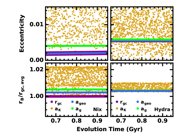
Figure 1: Time evolution of four estimates of the semimajor axis (lower panels) and the eccentricity (upper panels) for Nix (left panels) and Hydra (right panels) for a calculations with $f_{H}$ = 1.1. Other satellites have their nominal masses. The legends in the lower panels map colors to each estimate. The upper panels use the same color scheme as the lower panels. In each panel, estimates derived from the restricted three-body theory yield the best results for $a$ and $e$.

The lower panels of Fig. 1 also compare the two geometric estimates of the semimajor axis, $a_{g}$ and $a_{geo}$, with $r_{gc}$. Because $r_{gc}$ tracks a circular orbit with $e_{free}$ = 0, $a_{g}$ and $a_{geo}$ are larger than $r_{gc}$ when $e_{free}$ is larger than zero. In the Nix example, the orbital excursions due to the binary potential (i.e., $\Delta R_{+}$ and $\Delta R_{-}$) are large, $\sim$ 0.01–0.03 $R_{P}$. Taking these excursions into account places $a_{geo}$ inside $a_{g}$. Moving outward in the system to Hydra, $\Delta R_{+}$ and $\Delta R_{-}$ are smaller, $\lesssim$ 0.005 $R_{P}$. While $a_{geo}$ still lies inside $a_{g}$, the difference is not obvious in the Figure.

The upper panels of Fig. 1 demonstrate that $e_{free}$ and $e_{geo}$ yield similar results for the eccentricity of Nix’s orbit. Measurements of $e_{free}$ are variable at the $\pm$0.0004 level due to the accuracy limitation of the estimator (see Fig. 3 of Bromley & Kenyon, 2021); $e_{geo}$ is nearly constant in time. The $e_{g}$ values are a factor of two larger and also roughly constant in time. Once again the Keplerian estimate $e_{K}$ is nearly random; even the median of $e_{K}$ provides a poor measure of the eccentricity.

For the orbit of Hydra, three estimates – $e_{g}$, $e_{geo}$, and $e_{free}$ – are essentially identical. Estimates based on the restricted three body model, $e_{geo}$ and $e_{free}$, are indistinguishable and vary little in time. The basic geometric value is somewhat larger. Although the Keplerian approach yields a more accurate semimajor axis for Hydra than for the other satellites, the eccentricity measure is not useful.

As with the semimajor axis, the Keplerian eccentricity is more accurate for orbits more distant from the barycenter. Because $e$ is more sensitive to the binary potential than $a$, we recommend using the energy and angular momentum equations for $a$ and $e$ only for orbits with $a_{K}\gtrsim$ 600 $R_{P}$. Between 100 $R_{P}$ and 600 $R_{P}$, $a_{g}$ and $e_{g}$ are fairly reliable. Inside of 100 $R_{P}$, we prefer the three-body estimates.

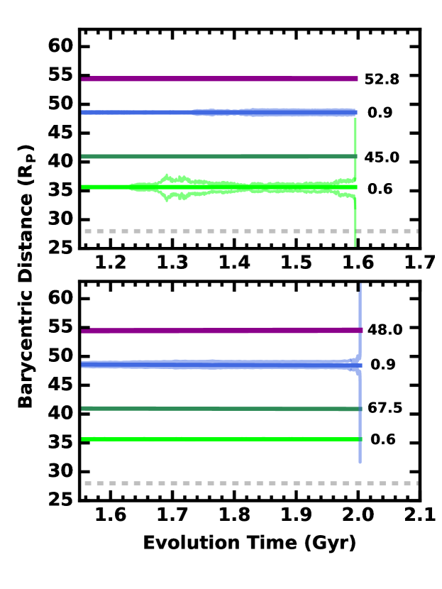
Figure 2: Time evolution of the barycentric distance for Styx (light green), Nix (dark green), Kerberos (blue), and Hydra (purple). The very light green (blue) curve plots $q_{S}$ and $Q_{S}$ ($q_{K}$ and $Q_{K}$) as defined in the text. The horizontal dashed grey line near the bottom of each panel indicates the location of the innermost stable distance for circular orbits in the orbital plane of the central binary (Kenyon & Bromley, 2019b). The masses (in units of $10^{18}$ g) for each satellite in the simulation are listed to the right of each curve.

Fig. 2 illustrates the time evolution of the barycentric distance of the four satellites. Lighter curves in each panel plot $q_{i}$ and $Q_{i}$. In every calculation, the more massive Nix and Hydra perturb the orbits of Styx and Kerberos. Sometimes the perturbations are small; variations in the barycentric distances of Styx and Kerberos are roughly constant in time. In other cases, oscillations $r_{gc}$  $q$, and $Q$ steadily grow with time. When the combined mass of the satellite system is several times the nominal combined mass, orbits evolve rapidly; Styx or Kerberos or both are ejected. Systems with a mass closer to the nominal combined mass evolve very slowly. However, the excitations eventually cross a threshold, becoming more dramatic with every orbit. At least one of the small satellites is then ejected from the system.

In the top panel of Fig. 2, Hydra has a mass 10% larger than its nominal mass. Other satellites have their nominal masses. During the first Gyr of evolution, oscillations in $q$ and $Q$ for Styx and Kerberos are fairly stable. At $\sim$ 1.25 Gyr, oscillations in the orbit of Styx become more obvious. Although it seems likely at this point that Styx will soon cross the orbit of Nix, the orbit gradually recovers and returns to a low $e$ for the next 250 Myr. During this period, the orbit of Kerberos develops a modest eccentricity. Eventually, Styx crosses the orbits of Nix and Kerberos and ventures well inside the unstable region. The central binary then ejects it from the system.

The lower panel of Fig. 2 shows an example where the mass of Nix is 50% larger than its nominal mass. Other satellites have their nominal masses. For roughly 1.5 Gyr, oscillations in the orbit of Kerberos are steady. In response to the larger mass of Nix, the orbit of Styx moves slightly closer to the system barycenter. Oscillations in this orbit are modest and also remain roughly constant in time. At $\sim$ 2 Gyr, oscillations in Kerberos’ orbit grow rapidly. Unlike the example in the top panel of Fig. 2, Kerberos does not excite fluctuations in Styx’s orbit. The oscillations in Kerberos’ orbit simply grow until Kerberos crosses the orbits of Nix and Hydra. Gravitational kicks from Nix and Hydra eventually push Kerberos well inside the unstable region surrounding the central binary, which ejects it from the system.

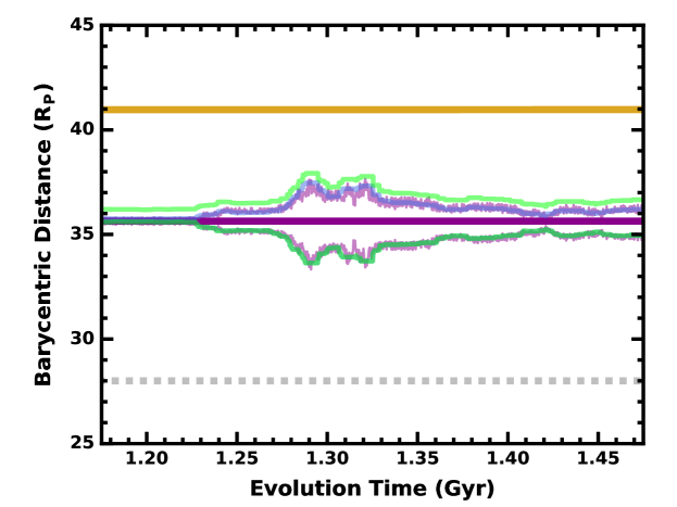
Figure 3: Expanded view of the time evolution of the barycentric distance for Styx and Nix from the top panel of Fig. 2, where $f_{H}$ = 1.1. Other satellites have their nominal masses. The light tan curve shows the orbit of Nix. For the orbit of Styx, the dark purple curve plots $r_{gc}$; $q$ and $Q$ are shown for the basic geometric model (light green), the geometric solution from the restricted three-body problem (blue), and for the model for $e_{free}$ (light purple). The basic geometric values have a larger excursion in the orbit than values derived from the restricted three-body problem.

Fig. 3 illustrates the evolution of $q_{S}$ and $Q_{S}$ in an expanded version of the top panel of Fig 2. Throughout this part of the evolution, $r_{gc}$ (dark purple curve) is nearly constant in time. At $\sim$ 1.23 Gyr, $q_{gc}$ and $Q_{gc}$ (light purple curves) begin to grow, each reaching $\sim$ 2 $R_{P}$ from $r_{gc}$ ($e_{free}$ $\approx$ 0.06). After $\sim$ 50 Myr, $q_{gc}$ and $Q_{gc}$ begin a long decline and then undergo and smaller oscillation on a longer times scale. During the main oscillation in $q_{gc}$ and $Q_{gc}$, $r_{gc}$ moves slightly inward and then returns to its original value.

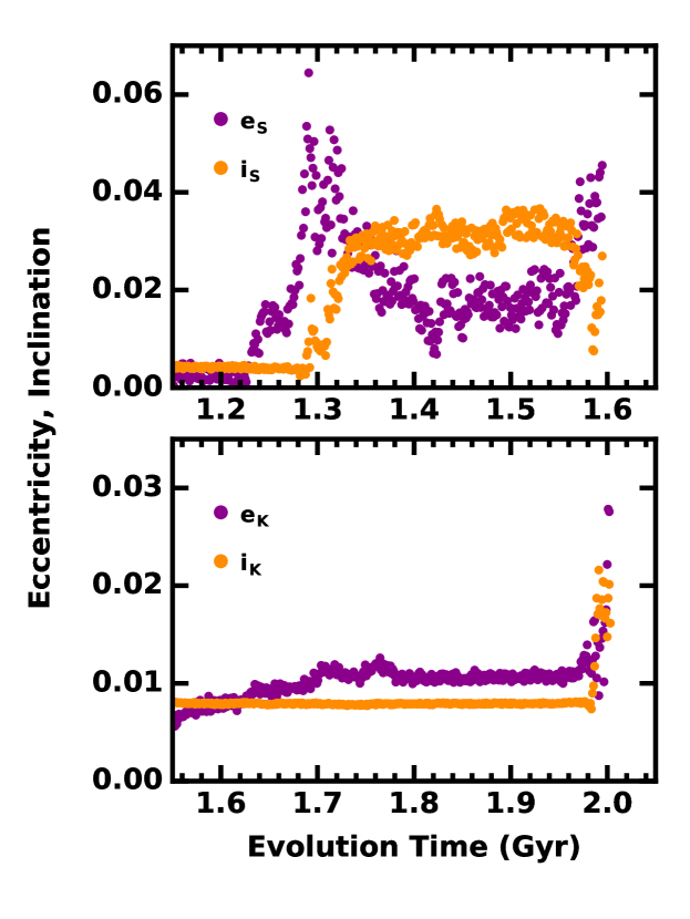
Figure 4: Time variation of $e_{free}$ and $\imath$ for Kerberos (lower panel, from the calculation shown in the lower panel of Fig. 2) and Styx (upper panel, from the calculation shown in the upper panel of Fig. 2). In the lower panel, the orbital inclination of Kerberos is approximately constant for nearly 2 Gyr and then rises abruptly just before Kerberos is ejected. In the upper panel, the inclination of Styx begins to rise when $e$ reaches a maximum level and then finds a plateau as $e$ returns to a stable value. Once $e$ rises again, $\imath$ drops; Styx is then ejected.

Other curves in this Figure show the variation of $q_{geo}$ and $Q_{geo}$ (light blue curves) and $q_{g}$ and Qg (light green curves). Throughout this time sequence, pericenter and apocenter derived from the basic geometric model have larger fluctuations than those estimated from the restricted three-body model. The $a_{geo}$ and $Q_{geo}$ values track the guiding center values very closely and have somewhat smaller fluctuations.

All of these estimates yield a much better characterization of the orbit than the Keplerian estimates derived from eqs. 1–2. With $a_{K}$ and $e_{K}$, the pericenter of Styx’ orbit sometimes passes close to or inside the unstable region surrounding the binary; at these times, apocenter passes dangerously close to Nix. This behavior is a function of the non-spherical potential of the central binary, which generates small radial excursions in the orbit and can ‘fool’ the Keplerian estimators into thinking Styx is much closer to Nix than it actually is.

Although the basic and more advanced geometric estimates track the orbit well, it is important to take some care in setting the appropriate window to derive $R_{min}$ and $R_{max}$ from a time sequence within an $n$-body calculation (see also Sutherland & Kratter, 2019). Here, we used a time-centered approach, inferring $R_{min}$ and $R_{max}$ from 100 samples before and another 100 samples after a given time $t$. While fewer samples enable accurate estimates of $a_{g}$ or $a_{geo}$, they also resulted in smaller differences between $q$ and $Q$. Among the set of calculations analyzed for this paper, larger samples did not change the results significantly.

To understand the behavior in the evolution of Styx and Kerberos in Fig.2, we consider the variation in $e$ and $\imath$ (Fig. 4). In the calculation where Kerberos is ejected (lower panel), $e$ slowly rises from $\sim$ 0.005 at 1.5 Gyr to 0.011 at 1.8 Gyr, remains roughly constant for $\sim$ 170 Myr, and then rises dramatically as Kerberos is ejected (Fig. 4). In contrast, $\imath$ is nearly constant at 0.0078 for 1.98 Gyr, drops somewhat as $e$ begins to grow, and then follows the dramatic increase in $e$ as Kerberos crosses the orbits of Nix and Hydra, ventures into the unstable zone close to Pluto–Charon, and is then ejected.

The evolution of Styx in the upper panel of Fig. 4 is more interesting. Well before ejection, the orbital eccentricity of Styx first grows dramatically and then varies between 0.03 and 0.06 at 1.22–1.32 Gyr. During this period, Styx has not crossed the orbit of Nix or the innermost circumbinary orbit, but a much larger growth in $e$ would place Styx in peril. Just after $e$ reaches a maximum, $\imath$ begins to rise and reaches a maximum of $\imath\approx$ 0.03 at $\sim$ 1.34 Gyr. During this period $e$ drops to 0.01–0.02 and maintains this level for close to 200 Myr. Eventually, the eccentricity begins to grow (and the inclination drops). Styx is then ejected.

Among the $\sim$ 300 calculations where the combined mass of the satellites is no more than twice the total nominal mass, all follow one of the two paths summarized in Fig. 4. In most systems, $e_{S}$ or $e_{K}$ slowly rises with little or no change in $\imath_{S}$ or $\imath_{K}$. Eventually, the eccentricity of one satellites begins to grow dramatically; $\imath$ then rises to similar levels and the satellite is ejected. In other calculations, a satellite maintains a large $\imath$ for a long period before an ejection. In these cases, the growth of $\imath$ allows the satellite to avoid Nix and Hydra, stabilizing the satellite’s orbit for many Myr. Eventually, perturbations from Nix and Hydra induce the satellite to cross into the unstable region close to the binary and the satellite is ejected.

2.6 Collision Rates

In all calculations where the $n$-body code resolves collisions, small satellites are ejected before they collide with one another. Combining the examples in the previous section with the orbital architecture, we demonstrate that physical collisions are unlikely. We approximate the orbits of Styx/Kerberos (Nix/Hydra) as coplanar ellipses (circles) relative to the system barycenter. Collisions only occur near the apocenters of the orbits of Styx (for collisions with Nix) and Kerberos (for collisions with Hydra). Defining a time period $\Delta t$ when a collision is possible, the probability a satellite with orbital period $P_{i}$ occupies that part of its orbit is $\Delta t/P_{i}$. The other satellite with orbital period $P_{j}$ occupies this region once per orbit. Thus, the collision probability is

$$p_{coll}=\frac{2\Delta t}{P_{i}P_{j}}~{},$$ (9)

where the factor of two results from two crossings per orbital period $P$.

For a quantitative estimate of $\Delta t$, we consider the equation of the barycentric distance of an elliptical orbit for Styx or Kerberos, $r_{i}=a_{i}(1-e_{i}^{2})/(1+e~{}{\rm cos}~{}\theta_{i})$. Here, the angle $\theta_{i}$ is measured counterclockwise from the $x$-axis in the orbital plane. Defining $R_{tot}=R_{i}+R_{j}$ as the sum of the physical radii, we seek solutions for $\theta_{i}$ where the small satellite has a distance from the barycenter

$$a_{j}-R_{tot}\leq r_{i}\leq a_{j}+R_{tot}$$ (10)

For an adopted $e_{i}$, it is straightforward to solve for the two angles that define the minimum, $\theta_{i,min}$, and maximum, $\theta_{i,max}$ distances where collisions can occur. The interaction time $\Delta t_{i}$ follows from $\Delta\theta_{i}=\theta_{i,max}-\theta_{i,min}$ and application of Kepler’s second law.

These solutions suggest the typical interaction time $\Delta t$ is small. When Styx has $e_{S}\leq$ 0.1409, collisions cannot occur. As $e_{S}$ grows from 0.141 to 0.1422, $\Delta t$ rises from $\sim$ 50 sec to $\sim$ 1650 sec. For larger $e_{S}$, the interaction time is a slowly decreasing function of $e_{S}$. When Kerberos has $e_{K}\leq$ 0.1199, collisions with Hydra are impossible. This system has a maximum $\Delta t\approx$ 2500 sec for $e_{K}$ = 0.1209 and a slowly decreasing $\Delta t$ at larger $e_{K}$. In both cases, the maximum interaction time is at apocenter. The corresponding collision probabilities are $p_{coll}\approx 0.0019$ per Nix orbit for collisions with Styx and $p_{coll}\approx 0.0018$ per Hydra orbit for collisions with Kerberos. The time scale from orbit crossing to ejection is typically a few orbits of Nix or Hydra. Thus, the likelihood of a physical collision is small.

Other approaches to derive $\Delta t$ yield similar results (e.g., Opik, 1951; Wetherill, 1967; Rickman et al., 2014; JeongAhn & Malhotra, 2017). All express the probability of a collision in a form similar to eq. 9. Our method has the advantage of avoiding linear or parabolic approximations to the trajectories for analytical solutions and the intricacies of more involved numerical estimates. Although we ignore the exact shape of a circumbinary orbit, corrections due to the circumbinary potential should be small.

Generalizing the method to an elliptical orbit for the more massive target and an inclined orbit for the impactor is straightforward. Elliptical orbits for Nix/Hydra do not change the probabilities significantly. At apocenter, Styx (Kerberos) lies at a height $z_{S}$ ($z_{K}$) above the orbital plane of Nix (Hydra), where $z_{i}=a_{i}~{}{\rm sin}(\imath_{i}-\imath_{j})$. Requiring $|z_{i}|\leq R_{tot}$ when orbits cross implies $\Delta\imath=|\imath_{i}-\imath_{j}|\leq$ 0.001 (0.00077) for Styx–Nix (Kerberos–Hydra) collisions. At the start of each calculation $\Delta\imath\approx$ 0.0029 for Styx–Nix and 0.0028 for Kerberos–Hydra. In all of the calculations, the inclination difference between Styx–Nix and Kerberos–Hydra grows with time. Thus, physical collisions among the small satellites are impossible.

Despite the lack of physical collisions, orbit crossings often place Styx (Kerberos) within the Hill sphere of Nix (Hydra). Replacing $R_{tot}$ in eq. 10 with the radius of the Nix or Hydra Hill sphere results in factor of ten larger probabilities for strong dynamical interactions instead of physical collisions when Styx or Kerberos are at apocenter. The large satellite inclinations $\Delta\imath\approx$ 0.01 also place Styx (Kerberos) on the edge of the Nix (Hydra) Hill sphere during orbit crossings. Entering the Hill spheres of Nix and Hydra provide additional perturbations to the orbits of Styx and Kerberos.

In the next section, we discuss results from the ensemble of $n$-body calculations. After examining the ejection frequency for Styx and Kerberos as a function of initial system mass, we derive the frequency of systems where $\imath$ maintains an elevated level prior to ejection. We conclude with new estimates of the total system mass and illustrate the impact of the masses of Styx and Kerberos on the ejection time scale.

3 Results

Once a calculation begins, all of the evolutionary sequences follow the same trend. After a period of relative stability where the orbital parameters of the system are roughly constant in time, the motion of at least one satellite begins to deviate from its original orbit. These deviations grow larger and larger until the orbits cross the 3:1 (Styx) or the 5:1 (Kerberos) resonance with the central binary. After resonance crossing, orbits are excited to larger $e$ and $\imath$. Although Styx and Kerberos can maintain a state of higher $e$ and $\imath$ for awhile, resonance crossing and perturbations by Nix and Hydra eventually lead to orbit-crossings. After orbits begin to cross, the motion of either Styx or Kerberos rapidly carries it inside the region close to Pluto–Charon where circumbinary orbits are unstable. After a few passes, at least one satellite – usually Styx or Kerberos – is ejected from the system.

3.1 Ejection Statistics

To examine ejection statistics for the ensemble of $n$-body calculations, we begin with a brief summary of the model parameters. In one set of calculations, we vary the mass of Nix or Hydra and set other satellites at their nominal masses. As summarized in Table 2, we have 38 (50) completed calculations for $f_{N}>1$ ($f_{H}>$ 1). The character of the evolution changes when Hydra or Nix are more than twice their nominal masses. Thus, we consider two sets of results for each model sequence.

In the calculations where the masses of all satellites are multiplied by the same factor $f$, we have sets with $f_{s}=f_{K}$ = 1.0, 1.5, 2.0, and 3. For $f\geq$ 1.5, nearly all calculations are complete. While most with $f$ = 1.25 are complete, only 10 with $f$ = 1 have finished. Comparisons among the sets with $f\geq 1.5$ indicates that ejection frequencies are independent of $f_{S}$ and $f_{K}$. Thus, we combine statistics into one row of Table 2. For simplicity, we follow this procedure for sets with $f$ = 1.00 and 1.25.

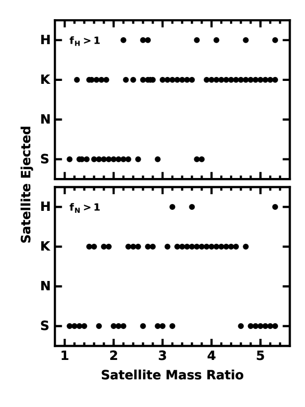
Figure 5: Ejection diagram for calculations with $f_{N}>1$ (lower panel) and $f_{H}>1$; other satellites have their nominal masses. Letters on the y-axis correspond to the satellites, with ‘S’ for Styx, ‘N’ for Nix, ‘K’ for Kerberos, and ’H’ for Hydra. Nix is never ejected. Hydra ejections only occur in very massive systems. Kerberos is usually ejected when Hydra is massive. A massive Nix ejects either Styx or Kerberos roughly half of the time.

Figure 5 illustrates results for the full set of calculations with $f_{N}>1$ (lower panel) and $f_{H}>1$ (upper panel). At the largest masses in the lower panel, Kerberos is rarely ejected. Among systems with slightly smaller masses, $f_{N}$ = 3.0–4.5, Kerberos is almost always ejected. At still lower masses, Styx and Kerberos have similar ejection probabilities. Styx ejections dominate the lowest masses. Kerberos ejections dominate the set of calculations with $f_{H}>1$ in the upper panel. Among the more massive systems with $f_{H}>2$, Styx ejections are rare. Below this limit, Styx ejections dominate.

Surprisingly, ejections of Styx or Kerberos are sometimes accompanied by an ejection of Hydra. Nix is never ejected. Of the ten calculations where Hydra is ejected, Styx accompanies Hydra out of the Pluto–Charon system 4 times. All of these systems have massive satellites with $f_{N}>2$ or $f_{H}>2$ and follow a common pattern. Once Styx (Kerberos) begins to cross the orbit of Nix (Hydra), Hydra’s orbit begins a small oscillation, crosses the 3:2 resonance with Nix at pericenter, develops a much larger oscillation in its orbit, and is then ejected.

To supplement Fig. 5, the first four rows of Table 2 summarize the frequency of Styx, Kerberos, and Hydra ejections in this set of calculations. The dominance of Kerberos (Styx) ejections at large (small) systems masses has a simple physical explanation in Hill space. In massive systems with $f_{H}>2$ or $f_{N}>2$, the satellite with the smallest $K$ (Kerberos) is most prone to develop oscillations that lead to orbit crossings. Lower mass systems with $f_{H}<2$ or $f_{N}<2$ always have $K>8$ and thus meet the minimum criterion for stability. Here, Styx’s lower mass and proximity to the innermost stable orbit make it a better candidate for ejection.

Table 2: Ejection Fractions

Model	N	Styx	Nix	Kerberos	Hydra
$f_{N}>2$	29	0.34	0.00	0.66	0.10
$f_{N}\leq 2$	9	0.67	0.00	0.33	0.00
$f_{H}>2$	35	0.20	0.00	0.80	0.20
$f_{H}\leq 2$	15	0.53	0.00	0.47	0.00
$f$ = 1.00	10	0.80	0.00	0.20	0.00
$f$ = 1.25	44	0.24	0.00	0.76	0.00
$f$ = 1.50	63	0.32	0.00	0.68	0.00
$f$ = 2.00	67	0.28	0.00	0.73	0.01

These considerations hold in the larger set of calculations with a fixed $f$ for all four satellites (Table 2, rows 5–8). In massive systems ($f$ = 1.25, 1.5 and 2), Kerberos is usually ejected. Styx dominates ejections for $f$ = 1, but the sample size is smaller. The lone calculation with a Hydra ejection occurs when $f$ = 2. Another $f$ = 2 calculation is the only one where Styx and Kerberos are ejected.

3.2 Signals

Fig. 4 illustrates two classes of evolutionary sequences in the $n$-body calculations. Often, the eccentricity of Styx or Kerberos gradually increases until the satellite starts to cross the orbit of one of the massive satellites. The satellite is then scattered across the innermost stable orbit, where Pluto–Charon eject it from the system. In other sequences, $e$ grows but stops short of orbit crossing due to a substantial increase in the inclination which reduces $e$. The system remains in this state for awhile before the high inclination satellite begins another foray at high $e$. This time, the satellite is ejected.

To understand the frequency of the two different types of sequences, we examine the evolutionary history of each $n$-body calculation with $f\leq 1.5$, $f_{N}\leq 2$, or $f_{H}\leq$ 2. For each of the 140 calculations in this sample, we derive the average $e$ and $\imath$ during the first 5% to 10% of the sequence. This exercise yields $(e_{i},\imath_{i})$ = (0.0073, 0.0044) for Styx and (0.0042, 0.0077) for Kerberos. For the satellite to be ejected at the end of the time sequence, we then search for the first time $t_{0}$ where $\imath$ rises above 0.01 after $e$ exceeds 0.01. With $t_{0}$ established, we verify that $e$ and $\imath$ are more than 10$\sigma$ larger than the average values and that both remain larger than 0.01 until a satellite is ejected. We define the fractional delay in an ejection as $D=(t_{0}-t_{f})/t_{f}$, where $t_{f}$ is the time the satellite leaves the Pluto–Charon system.

In addition to identifying $t_{0}$ and $D$, we investigate the maximum $e$ and $\imath$ for ejected satellites prior to ejection. In systems with small $D$, the maximum inclination for Styx is 0.01–0.02. When $D$ is large, Styx’s $\imath$ also tends larger, 0.05–0.10. Several time steps before ejection, $e\approx\imath$; in these cases, Styx follows an evolution similar to that in Fig. 4 where an increase in $e$ generates a rise in $\imath$. For Kerberos, there is little correlation between $D$ and values of $e$ and $\imath$ before ejection.

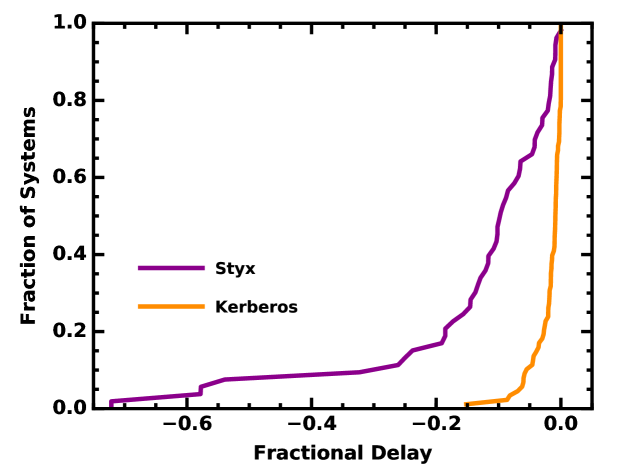
Figure 6: Cumulative distribution of the fractional time delay between the time when $\imath$ first rises above 0.01 and the time of ejection. In systems where Kerberos is ejected (orange curve), $\imath$ typically becomes larger than 0.01 just prior to ejection. When Styx is ejected, $\imath$ is often large well before ejection.

Fig. 6 shows the cumulative distribution of time delays for Styx (purple curve) and Kerberos (orange curve). Kerberos rarely produces a significant ‘signal’ that it will eventually be ejected. In $\sim$ 20% of the ejections, Kerberos does not signal at all: $\imath$ rises above 0.01 in the time step immediately prceeding the ejection. In another 37%, the delay is extremely short with $t_{0}\gtrsim 0.99~{}t_{f}$. In the remaining sequences, the delay is 1% to 10% of the system lifetime; the longest delay is 15%.

In contrast, Styx almost always provides a robust signal for its impending ejection. In only 10% of the ejections, Styx’s signal is weak with $t_{0}\gtrsim$ 0.99 $t_{f}$. Roughly half of the calculations find Styx with $\imath\gtrsim$ 0.01 at a time 10% or more before $t_{f}$. In some remarkable cases, Styx has a large $e$ and $\imath$ when $t_{0}\lesssim 0.5~{}t_{f}$. Somehow, these systems stay on the edge of instability for extended periods of time before an ejection.

In nearly all of these examples, the low mass satellite that is not ejected maintains much smaller $e$ and $\imath$ throughout the period where the other satellite is on the verge of ejection. Only one calculation has an ejection of Kerberos and Styx. Among the set of calculations with an ejection of Kerberos, Styx never has time to react to the orbital gyrations of Kerberos. After the orbit of Kerberos is perturbed, it rushes to an ejection. When Styx is to be ejected, Kerberos often reacts slightly to Styx’s oscillations in $e$ and $\imath$. Curiously, these never lead to ejection. As Styx leaves the system, Kerberos maintains a stable orbit.

The difference between Styx and Kerberos in Fig. 6 is probably a function of orbital separation in Hill units, $K$. As the satellite with the smallest $K$ and flanked by two massive satellites, Kerberos is closest to ejection at the start of each calculation. Small kicks from either Nix or Hydra are sufficient to increase $e$ and $\imath$ above 0.01. When that occurs, ejection rapidly follows. As discussed above, Styx has more room for its orbit to fluctuate. Despite its proximity to the innermost stable orbit, it can more easily trade off $\imath$ for $e$ and remain on the edge of ejection for many years.

3.3 Constraints on the System Mass

In Kenyon & Bromley (2019a), we considered the evolution of ‘heavy’ satellite systems, where Nix and Hydra have the masses listed in Table 1 and the masses of Styx ($4.5\times 10^{18}$ g) and Kerberos ($1.65\times 10^{19}$ g) are consistent with those reported in Brozović et al. (2015). With lifetimes $\tau_{i}\approx$ 100 Myr to 1 Gyr from eleven calculations, systems with these masses appeared to be unstable. In an analysis of three ongoing calculations, trends in the evolution of the $e_{g}$ and $a_{g}$ for Styx and Kerberos suggested these systems are also unstable. With likely $\tau_{i}\lesssim$ 2 Gyr, heavy satellite systems with the nominal masses derived from HST observations are unstable on time scales much smaller than the age of the solar system.

Kenyon & Bromley (2019a) also examined the evolution of ‘light’ satellite systems with the masses listed in Table 1. Calculations with $f$ = 2 (1.5) had median $\tau_{i}\approx$ 100 Myr (600 Myr). Several additional complete simulations for the present paper result in $\tau_{i}\lesssim$ 3 Gyr for all systems with $f$ = 1.5. For models with $f$ = 1.25, two calculations had $\tau_{i}$ = 700–850 Myr; trends in the evolution of $r$ with time suggested intact systems would be unstable on time scales of 3–4 Gyr. Although all but one of the calculations with $f$ = 1.0 had completed 1 Gyr of evolution with no ejections, the evolution of the orbits of Styx and Kerberos suggested some were unstable.

Since the publication of Kenyon & Bromley (2019a), the completion of many additional calculations improves the constraints on heavy satellite systems. All sixteen calculations with $f$ = 1 eject at least one satellite on time scales $\lesssim$ 2 Gyr.

For light satellite systems, we divide calculations into three groups: (i) at least one satellite has been ejected, (ii) at least one satellite has $e\gtrsim$ 0.01 or $\imath$ $\gtrsim$ 0.01 without an ejection, and (iii) all satellites have $e$ and $\imath$ close to their ‘nominal’ values and none have been ejected. The separation into the second and third groups is based on a set of calculations with $f$ = 0.5 where the satellites show no evidence of perturbations over 1 Gyr of evolution. Within this set, the time variation of the inclination is very small: $\imath$ = 0.00406–0.00485 with an average $\imath$ = 0.00445 for Styx and $\imath$ = 0.00764–0.00787 with an average $\imath$ = 0.00776 for Kerberos. Variations in eccentricity are only somewhat larger: $e_{free}\lesssim$ 0.004 with an average $e_{free}$ = 0.002 for Styx and $e_{free}$ = 0.002–0.004 with an average $e_{free}$ = 0.003 for Kerberos. Limits on the eccentricity from $e_{g}$ and $e_{geo}$ are similar. Orbits of Styx or Kerberos with $e\gtrsim$ 0.01 and $\imath\gtrsim$ 0.01 are not consistent with current observational limits from HST. We therefore reject these calculations (and their $f$ values) as possible matches to the Pluto–Charon system.

With this definition, the full set of completed $n$-body calculations yield strong limits on the combined satellite mass (Fig. 7). Within the suite of 18 simulations for $f$ = 2, lifetimes range from a minimum of $\tau_{i}\approx$ 20 Myr to a maximum of $\tau_{i}\approx$ 2 Gyr, with a median, $\tau_{i}\sim$ 170 Myr, roughly midway between the two extremes. Model systems with smaller $f$ have a smaller range in $\tau_{i}$. Among the 17 completed calculations with $f$ = 1.5, the maximum $\tau_{i}\sim$ 3 Gyr is only an order of magnitude larger than the minimum $\tau_{i}\sim$ 400 Myr. When $f$ = 1.25, $\tau_{i}$ spans 550 Myr to 3.5 Gyr among 16 calculations. As of this writing, 8 of 16 calculations with $f$ = 1.0 have measured $\tau_{i}$ = 0.6 Myr to 3.7 Gyr. Among the eight unfinished calculations that have reached $\sim$ 2–4 Gyr, none have $e_{S}$ or $e_{K}$ $\gtrsim$ 0.01. Thus half of the calculations with $f$ = 1 are consistent with HST observations; the other half are not.

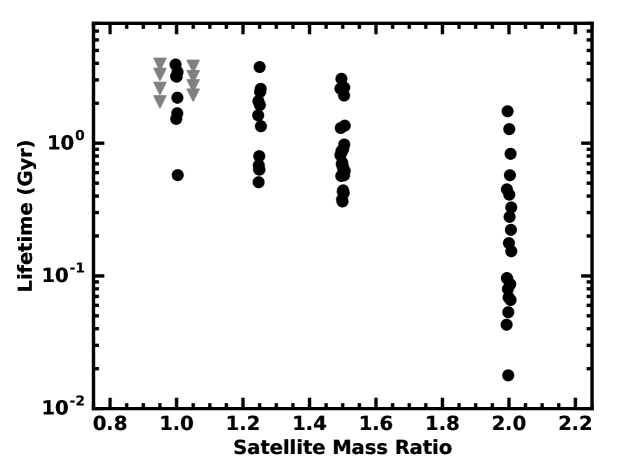
Figure 7: Lifetime of model Pluto–Charon satellite systems as a function of the mass ratio factor $f$. Satellites have masses $f$ times larger than the nominal masses listed in Table 1. Black dots indicate lifetimes for systems with ejections of either Styx or Kerberos. Grey triangles represent current lifetimes for eight ongoing calculations with $f$ = 1.0, which we include for completeness. Some points have been adjusted vertically or horizontally for clarity. More massive satellite systems typically have shorter lifetimes.

Based on calculations with at least one ejection, it is not possible to predict outcomes of the ongoing calculations with $f$ = 1. Because Kerberos rarely signals an impending ejection (Fig. 6), calculations with current lifetimes of 3–4 Gyr have time to eject Kerberos before 4.5 Gyr (when we plan to end each calculation). In roughly half of systems where Styx is ejected, Styx signals the outcome 0.1–0.5 Gyr before an ejection. Several ongoing calculations with $f$ = 1 have reached 3.5–4 Gyr; thus, there is time for a Styx ejection in these calculations.

3.4 Constraints on the Masses of Nix and Hydra

In addition to sets of calculations with masses $f$ times larger than the nominal masses, we performed calculations where either Nix or Hydra has a mass $f_{N}$ or $f_{H}$ times its nominal mass and other satellites have their nominal masses. Kenyon & Bromley (2019a) reported results for completed calculations with $(f_{N},f_{H})$ = 1.1–5 in steps of 0.1. In this range, 77 calculations produced an ejection; another 19 systems had evolved for at least 1 Gyr without an ejection. For each of the ongoing calculations, Kenyon & Bromley (2019a) used the time variation of $a_{g}$ and $e_{g}$ for Styx and Kerberos to estimate the likely stability of the system over 4.5 Gyr. Only one ongoing calculation was deemed stable.

Among the ongoing calculations in Kenyon & Bromley (2019a), all but three have resulted in an ejection (Fig. 8). With these results, we improve limits on the masses of Nix and Hydra. Of the 10 unfinished calculations with $f_{N}>1$ and $f_{H}$ = 1 from Kenyon & Bromley (2019a), all resulted in an ejection; the maximum lifetime is $\tau_{N}\lesssim$ 2.7 Gyr. Thus, the nominal mass listed in Table 1 provides a robust upper limit to the mass of Nix.

Of the nine previously unfinished calculations with $f_{N}$ = 1 and $f_{H}>1$, six resulted in an ejection. The range in lifetimes is 1–2.1 Gyr. In this set, the three unfinished calculations have $f_{H}$ = 1.2, 1.3, and 1.4 and evolution times of 3.6–3.8 Gyr. In two of these three ($f_{H}$ = 1.2 and 1.3, indicated by the filled orange triangles in Fig. 8), Kerberos has a steadily increasing $e\gtrsim$ 0.01; $\imath$ is also larger than 0.01. Thus, these systems provide poor matches to the orbital elements of the current Pluto–Charon satellite system. The rates of change of $e$ and $\imath$ in these calculations suggest ejections will occur before 4.5 Gyr.

In the calculation with $f_{H}$ = 1.4 (Fig. 8, filled orange star), the orbital eccentricities and inclinations of Styx and Kerberos vary more than calculations with $f$ = 0.5, but they do not reach the level of 0.01 that would be much too large to match the observed orbital elements. Thus, this system might end up matching the real satellite system. Even if this model system remains stable, the mass of Hydra is unlikely to exceed its nominal mass. With eight ejections for $f$ = 1, ejections for $f_{H}$ = 1.1 and $\gtrsim$ 1.5, and poor matches to the real Pluto–Charon system for $f_{H}$ = 1.2 and 1.3, the most likely mass for Hydra is less than or equal to its nominal mass.

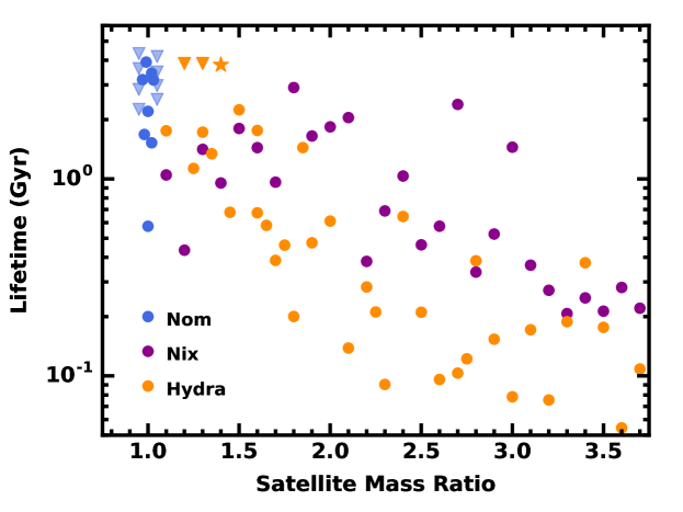
Figure 8: As in Fig. 7 for model Pluto–Charon satellite systems with a factor $f_{N,H}$ times the nominal mass for either Nix ($f_{N}>1$, purple dots) or Hydra ($f_{H}>1$, orange dots) and nominal masses for the other satellites. Blue dots indicate lifetimes of systems with the nominal masses for all satellites and one or more ejections. Orange stars indicate systems with $f_{H}>1$ where Kerberos has $e$ and $\imath$ much larger than derived from HST observations. For completeness, we include blue (orange) triangles to represent the range of lifetimes for eight (one) ongoing calculations with the nominal masses for all four satellites (with the nominal masses for Styx, Nix, and Kerberos and $f_{H}$ times the nominal mass for Hydra) where the system parameters still match orbital fits to HST observations. More massive satellite systems have shorter lifetimes.

3.5 Constraints on the Masses of Styx and Kerberos

To try to place initial constraints on the masses of Styx and Kerberos, we vary their masses independently of the masses of Nix and Hydra. For each calculation, we adopt $f_{S}$ = $f_{K}$ = 1.0, 1.5, 2.0, or 3.0 and then adopt $f$ = 1.0, 1.25, 1.5, 2.0, 2.5, and 3.0 for the full set of four satellites. As an example, when $f$ = 2 and $f_{S}=f_{K}$ = 1.5, Nix and Hydra have twice their nominal masses; Styx and Kerberos have thrice their nominal masses. Here, we discuss results for $f$ = 1.5–4.0 and defer consideration of calculations with $f$ = 1.0–1.25 to a later study.

The goal of this set of calculations is to learn whether the lifetimes of satellite systems with $f_{S}$ = 2–3 are significantly longer than the lifetimes of systems with $f_{S}$ = 1.0–1.5. When $f$ = 2.5 or 3.0, rapid ejections of Styx or Kerberos should make it difficult to measure different lifetimes in systems with different masses for Styx and Kerberos. These calculations serve to mimimize small number statistics in deriving a median lifetime. For smaller $f$, longer lifetimes enable tests to looks for differences among calculations with different $f_{S}$ and $f_{K}$.

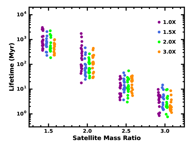
Figure 9: Lifetime of model Pluto–Charon satellite systems as a function of the mass ratio $f$ for different $f_{S,K}$. The legend indicates the adopted mass ratio $f_{S}=f_{K}$ for the masses of Styx and Kerberos relative to their nominal masses. For each calculation, Nix and Hydra have their nominal masses multiplied by the factor $f$; Styx and Kerberos have their nominal masses multiplied by $f*f_{S,K}$. For $f$ = 1.5–2, lifetimes for systems with larger mass ratios for Styx and Kerberos (e.g., $f_{S,K}$ = 2 or 3) have shorter lifetimes.

Fig. 9 plots the lifetimes of the satellite systems for calculations with $f$ = 1.5–3.0. Within each set, the typical range in lifetimes is a factor of $\sim$ 10. Curiously, the range is largest for simulations with $f$ = 2 for the nominal satellite masses. A larger set of calculations is required to learn whether this result is due to the small number of simulations or a real effect. For a complete suite of calculations with fixed $f_{S}$ and variable $f$, the lifetimes grow with decreasing $f$. Visually, the lifetimes for systems with $f$ = 1.5 appear smaller for larger $f_{S}$ than for smaller $f_{S}$.

Table 3 summarizes lifetimes for this suite of calculations. Aside from $f_{S}=f_{K}$ and $f$, the columns list the number of results for each combination of $f_{S}$ and $f$ and the minimum, median, and maximum lifetimes. Minimum lifetimes range from roughly 0.3 Myr for $f$ = 4 to 200–300 Myr for $f$ = 1.5. Maximum lifetimes are $\sim$ 10 times larger, ranging from 2–3 Myr for $f$ = 4 to 1–3 Gyr for $f$ = 1.5. Median lifetimes are roughly midway between the minimum and maximum values.

For large $f$ = 2–4, the minimum, median, and maximum lifetimes for a specific $f_{S}$ are rather uncorrelated. Systems with $f_{S}$ = 1 and $f_{S}$ = 3 have nearly identical values. Thus, the masses of Styx and Kerberos have little influence on the lifetimes of massive satellite systems. When $f$ is smaller, however, there is a systematic increase in the median and maximum lifetimes from $f_{S}$ = 3 to $f_{S}$ = 1. In these calculations, the masses of Styx and Kerberos clearly change the median lifetime.

To place the influence of Styx and Kerberos on a more quantitative footing, we compare the distributions of lifetimes for combinations of $f$ and $f_{s}$. We use the Python version of the Mann-Whitney–Wilcoxon rank-sum test, which ranks the lifetimes and uses a non-parametric technique to measure the probability that the two distributions are drawn from the same parent distribution. For $f$ = 2–4, the rank-sum probabilities are generally large, $\gtrsim$ 0.3, and indicate a correspondingly large probability that the distributions are drawn from the same parent population as suggested from the minimum, median, and maximum lifetimes in Table 3. For calculations with $f$ = 1.5, however, the rank-sum test returns a small probability, $p$ = 0.05, that calculations with $f_{S}$ = 1 and $f_{S}$ = 2 are drawn from the same population. The test returns a smaller probability, $p$ = 0.005, that the set of lifetimes for $f$ = 1 and $f$ = 3 are drawn from the same parent. Lifetimes for $f$ = 1 and $f$ = 1.5 have a high probability, $p$ = 0.29, of belonging to the same parent.

As a final check on these results, we consider the Python version of the non-parametric K–S test. This test leads to the same conclusions: high probabilities that lifetimes with $f\geq$ 2 for all $f_{S}$ are drawn from the same parent population and low probabilities that the set of lifetimes with $f$ = 1.5 and $f_{S}$ = 1 and either $f_{S}$ = 2 ($p$ = 0.07) or $f_{S}$ = 3 ($p$ = 0.08) are drawn from the same population.

Table 3: Lifetimes for Calculations with $f_{S}=f_{K}$ = 1–3

$f_{S},f_{K}$	$f$	N	$\tau_{min}$	$\tau_{m}$	$\tau_{max}$
1.0	4.0	15	13.001	13.251	13.674
1.0	3.5	15	13.160	13.467	13.890
1.0	3.0	17	13.430	14.179	14.487
1.0	2.5	16	14.065	14.600	15.015
1.0	2.0	19	14.750	15.685	16.740
1.0	1.5	19	16.060	16.342	16.984
1.5	4.0	15	13.047	13.525	13.839
1.5	3.5	15	13.085	13.601	14.096
1.5	3.0	15	13.667	14.100	14.666
1.5	2.5	16	14.065	14.563	15.158
1.5	2.0	16	14.892	15.352	16.167
1.5	1.5	14	15.859	16.300	16.817
2.0	4.0	15	12.992	13.370	13.908
2.0	3.5	16	13.262	13.739	14.463
2.0	3.0	15	13.382	13.853	14.485
2.0	2.5	17	13.978	14.585	15.236
2.0	2.0	18	14.949	15.315	15.922
2.0	1.5	15	15.766	16.155	16.852
3.0	4.0	15	13.068	13.389	13.637
3.0	3.5	15	13.268	13.578	13.931
3.0	3.0	15	13.554	13.771	14.434
3.0	2.5	15	14.237	14.828	15.036
3.0	2.0	18	14.961	15.568	16.146
3.0	1.5	14	15.868	16.127	16.496

Taken together, the results listed in Table 3 and from the K–S and rank-sum tests indicate that satellites systems with $f_{S}$ = 2–3 are more unstable than those with $f_{S}$ = 1.0–1.5. Because systems with the nominal masses and $f$ = 1 are barely stable, we conclude that lifetimes derived from the $n$-body calculations are sufficient to place limits on the masses of Styx and Kerberos, despite their small masses compared to Nix and Hydra. If this trend continues with the calculations for $f$ = 1.25 and $f$ = 1.0, then it should be possible to rule out systems where Nix and Hydra have their nominal masses but Styx and Kerberos are 2–3 times more massive than their nominal masses.

For this study, we conclude that Styx and Kerberos are more likely to have masses $\lesssim$ 1.5 times their nominal masses than $\gtrsim$ 2 times their nominal masses. For the dimensions measured from New Horizons (Weaver et al., 2016), the average bulk densities for Styx and Kerberos are then $\rho_{SK}\lesssim$ 1.5 $\rm g~{}cm^{-3}$, similar to the derived average bulk densities of Nix and Hydra (Kenyon & Bromley, 2019a).

Although stable satellite systems with smaller masses for Nix and Hydra and larger masses for Styx and Kerberos are possible, this option seems unlikely. Reducing the masses of Nix and Hydra below the nominal masses yields average bulk densities $\rho_{NH}\lesssim$ 1.25–1.30 $\rm g~{}cm^{-3}$. Allowing $f_{S}\approx f_{K}\gtrsim$ 2 establishes much larger average bulk densities for the smallest satellites, $\rho_{SK}\gtrsim$ 2 $\rm g~{}cm^{-3}$. If all four satellites grow out of debris from a giant impact (e.g., Canup, 2005, 2011; Arakawa et al., 2019; Bromley & Kenyon, 2020; Kenyon & Bromley, 2021), it is unclear why they should have such different bulk densities. Thus, we conclude that the combined system mass $m_{SNKH}\lesssim 9.5\times 10^{19}$ g favors bulk densities for Styx and Kerberos similar to those of Nix and Hydra.

4 Discussion

Together with measurement of $(e_{S},\imath_{S})$ and $(e_{K},\imath_{K})$ of several ongoing calculations, the $\sim$ 1200 completed $n$-body calculations described here and in Kenyon & Bromley (2019a) paint a clear picture for the masses of the four small satellites of Pluto–Charon. The marginal stability of systems with the nominal masses and the instability in nearly all systems with the nominal masses and either $f_{N}>$ 1 or $f_{H}>$ 1 set a strict upper limit on the combined mass of all four satellites, $M_{SNKH}\lesssim 9.5\times 10^{19}$ g. The rank-sum and KS tests indicate the masses of Styx and Kerberos are no more than twice their nominal masses. If these two small satellites have masses larger than their nominal masses, the masses of Nix and Hydra must be reduced to maintain the upper limit on the total system mass.

In Kenyon & Bromley (2019a), we derived probability distributions for the satellite bulk density with a Monte Carlo (MC) calculation. From New Horizons, the satellites have measured sizes and associated errors in three dimensions, e.g., $x_{k}\pm\delta x_{k}$, for three principal axes $k$ = 1, 2, 3 (Weaver et al., 2016). Defining the volume as some function of the dimensions, $V=f(x_{k})$, and assuming a gaussian distribution for the measurement errors, the MC analysis yields a probability distribution for the volume, e.g., $p(V_{n})$, where $n$ = 1–N is a Monte Carlo trial and $N=10^{4}$. For an adopted satellite mass $m_{n}$, the bulk density for each trial is $\rho_{n}=m_{n}/V_{n}$. We report the median of the bulk density distribution and adopt the inter-quartile range as a measure of the uncertainty in the median. Kenyon & Bromley (2019a) also described results for the bulk density derived from a probability distribution of satellite masses, $p(m_{n})$. Each MC trial then samples $p(m_{n})$ and $p(V_{n})$ to infer a probability distribution for $\rho_{n}$.

Compared to Kenyon & Bromley (2019a), we have stronger limits on the satellite masses for $f\geq 1$ and no additional information on masses for $f<1$. Thus, we derive bulk density estimates for the nominal masses in Table 1. Although Kenyon & Bromley (2019a) considered two options for errors in the size measurements from New Horizons, the bulk densities were fairly independent of plausible choices. We refer readers to Table 3 of Kenyon & Bromley (2019a) for bulk density estimates derived from adopted mass distributions and different choices for size errors.

Kenyon & Bromley (2019a) considered three possible shapes for the small satellites, boxes, triaxial ellipsoids, and pyramids. However, satellite images from New Horizons do not resemble boxes (where the volume is close to a maximum) or pyramids (where the volume is close to a minimum). Triaxial ellipsoids, where the volume $V=4\pi x_{1}x_{2}x_{3}/3$, are plausible shapes and have a volume intermediate between boxes and pyramids. For New Horizons images of the Kuiper Belt object (486958) Arrokoth, the best-fitting global shape model of each lobe closely resembles triaxial ellipsoids (Spencer et al., 2020). Thus, our choice for the Pluto–Charon satellites is reasonable.

With no new analysis of New Horizons images, we rely on the Kenyon & Bromley (2019a) MC estimate for the volumes of Nix and Hydra. Scaling the results for the improved limits on the mass yields a median bulk density, $\rho_{N}\approx$ 1.55 $\rm g~{}cm^{-3}$ for Nix and $\rho_{H}\approx$ 1.30 $\rm g~{}cm^{-3}$ for Hydra. Using the interquartile range, the error in the bulk density is $\pm$0.2 $\rm g~{}cm^{-3}$ for Nix and $\pm$0.4 $\rm g~{}cm^{-3}$ for Hydra. The large error for Hydra is a result of larger errors in the measured dimensions from New Horizons. The probability that the satellites have smaller bulk densities than Charon (Pluto) is 65% (80%) for Nix and 75% (90%) for Hydra. Hydra’s lower bulk density results in a higher probability of a bulk density that is lower than Charon’s or Pluto’s.

Given the uncertainties, the average bulk density of the four satellites is comparable to the average bulk density of Nix and Hydra, $\rho_{SNKH}\lesssim$ 1.4 $\rm g~{}cm^{-3}$. Plausible errors in this estimate are $\pm$0.1–0.2 $\rm g~{}cm^{-3}$. The shorter lifetimes of satellite systems with $f_{S,K}\gtrsim$ 2 point to similar bulk densities $\rho_{SK}\lesssim$ 1.5 $\rm g~{}cm^{-3}$ for Styx and Kerberos.

The bulk densities derived for the Pluto–Charon satellites are similar to the densities of other small objects in the solar system. Satellites of Mars, Saturn, and Uranus with similar sizes as Styx/Nix/Kerberos/Hydra have $\rho\approx$ 0.5–1.5 $\rm g~{}cm^{-3}$ (e.g., Jacobson & French, 2004; Renner et al., 2005; Jacobson, 2010; Pätzold et al., 2014; Chancia et al., 2017). Curiously, Kuiper belt objects (KBOs) with much larger radii, $r\approx$ 50–200 km, have much lower bulk densities, $\sim$ 0.5–1.0 $\rm g~{}cm^{-3}$; larger KBOs with $r\approx$ 500–1000 km have higher bulk densities, $\gtrsim$ 1.5 $\rm g~{}cm^{-3}$ (e.g., Brown, 2012; Grundy et al., 2019). Bulk density measurements of other satellites are needed to place the Pluto–Charon satellites in context with moons throughout the solar system.

In the inner solar system, high quality astrometric data provide evidence for rubble-pile structures in some asteroids (e.g., Chesley et al., 2014). Coupled with high quality modeling, these data suggest low bulk densities and high porosity. Bierson & Nimmo (2019) demonstrate that the variation in bulk density of KBOs could result from a variation in porosity, where smaller KBOs have a much larger porosity than larger KBOs. In this scenario, the additional mass of larger KBOs compacts the structure and generates a smaller porosity.

In the Pluto–Charon satellites, the bulk density estimates are based on an upper limit of the mass and a median volume derived from a probability distribution, $\rho=m/V_{med}$. In this approach, allowing for empty regions in each satellite has no impact on the overall bulk density. The derived masses and volumes are the same. However, a high degree of void in a satellite increases the bulk density of the non-void material. As an example, the porosity required for Pluto-like material with $\rho_{P}$ = 1.85 $\rm g~{}cm^{-3}$ to have the bulk density of Nix, $\rho_{N}\approx$ 1.55 $\rm g~{}cm^{-3}$, is 16%. For Hydra, the required porosity is 30%. In both satellites, the porosity required for non-void material to have the bulk density of Charon is smaller, $\sim$ 9% for Nix and $\sim$ 24% for Hydra. Porosities much larger than these estimates require satellite compositions dominated by rock, which seems unlikely.

Even with uncertainties regarding the porosity of the small satellites, the results described here provide stronger support that the satellites are icy material ejected (i) from Pluto during a giant impact that results in a binary planet (e.g., Canup, 2005, 2011; Kenyon & Bromley, 2021; Canup et al., 2021) or (ii) from a more modest impact between a trans-Neptunian object and Charon (Bromley & Kenyon, 2020). In models where Charon forms out of the debris from the giant impact (e.g., Desch, 2015; Desch & Neveu, 2017), the bulk densities of the small satellites are more likely to be similar to Charon than to the low densities derived here. In $n$-body simulations of Charon formation, dynamical interactions are unlikely to leave behind sufficient material for the small satellites (Kenyon & Bromley, 2019c).

In addition to limits on satellite masses and bulk densities, the suite of $n$-body calculations provide interesting information on the frequency of ejections and the prelude to an ejection. In systems with at least twice the nominal mass, Kerberos is ejected much more often than Styx. For lower mass systems, Styx ejections are more likely. Within the suite of calculations for systems with $f\leq$ 2, Styx often signals an upcoming ejection by developing a relatively large inclination, $\imath_{S}\gtrsim$ 0.01. Styx can remain at this inclination many Myr before an ejection.

This behavior is a natural outcome of the orbital architecture of the four small satellites. Because Kerberos–Styx has the smallest $K=(a_{i}-a_{j})/R_{H,ij}$, it is the most likely satellite to suffer orbital perturbations from Nix and Hydra. Kerberos is also the closer of the two smaller satellites to an orbital resonance with the central binary. Youdin et al. (2012) demonstrated that the 5:1 resonance with Pluto–Charon is unstable. Thus it is not surprising that Kerberos is more likely to be ejected than Styx in massive satellite systems.

The behavior of Styx in the $n$-body calculations is fascinating. Despite having a larger $K$ and orbiting farther away from an orbital resonance, it is often ejected in low mass satellite systems. Its ability to signal an ejection while maintaining a modest $\imath\approx$ 0.02–0.03 for several hundred Myr is a consequence of angular momentum conservation: when perturbations from Nix and Hydra increase $e_{S}$, the satellite is able to reduce $e$ (thus reducing perturbations) by raising $\imath$ and maintaining stability. Because Kerberos has a more precarious orbit, it does not have this option and rarely signals an upcoming ejection.

5 Summary

We analyze a new suite of $\sim$ 500 numerical $n$-body calculations to constrain the masses and bulk densities of the four small satellites of the Pluto–Charon system. To infer the semimajor axis and eccentricity of circumbinary satellites from the six phase-space coordinates from the $n$-body code, we consider four approaches. Keplerian elements derived from the orbital energy and angular momentum (eqs. 1–2) poorly represent circumbinary orbits. Two geometric estimates (eqs. 3–6) enable good results for long $n$-body integrations but also require good sampling over many orbits (see also Sutherland & Kratter, 2019). Geometric estimates based on restricted three-body theory yield somewhat smaller and more accurate measures of $a$ and $e$ for the Pluto–Charon satellites. An instantaneous estimate derived from the restricted three-body problem provides the radius of the guiding center $r_{gc}$ as a surrogate for $a$ and the free eccentricity $e_{free}$. For the Pluto–Charon satellites (especially Styx and Nix), $r_{gc}$ is a better measure of the semimajor axis than $a_{g}$ or $a_{geo}$; $e_{free}$ and $e_{geo}$ are roughly equivalent measures of the eccentricity.

Results from the new calculations build on the analysis of $\sim$ 700 simulations from Kenyon & Bromley (2019a). The earlier calculations demonstrated that heavy satellite systems – where the masses of Styx and Kerberos are much larger than those in Table 1 (Brozović et al., 2015) – are unstable. Another set of early calculations showed that light satellite systems with masses $f\geq$ 1.5 times larger than the nominal masses in Table 1 are also unstable. Finally, a third set of results yielded robust upper limits on the masses of Nix ($\leq$ twice the nominal mass) and Hydra ($\leq$ 1.5 times the nominal mass).

The analysis described here focuses solely on light satellite systems. Completed calculations with mass fractions (i) $f$ = 1.00–1.25 times the nominal mass of the combined satellite system, (ii) $f_{N}$ = 1–2 times the mass of Nix, and (iii) $f_{H}$ = 1.0–1.5 times the mass of Hydra place better constraints on the total system mass. We also derived new results for systems with 1.5–4 times the nominal masses of Nix and Hydra and 2.25–12 times the nominal masses of Styx and Kerberos to understand whether system lifetimes depend on the masses of the two smallest satellites.

When combined with the $\sim$ 700 simulations from Kenyon & Bromley (2019a), we draw the following conclusions.

• When the mass of the satellite system is more than twice the nominal mass (Table 1, Kerberos is ejected more often than Styx. In lower mass systems, Styx is more likely to be lost than Kerberos. In either case, ejections occur when Nix or Hydra (or both) perturb the orbit of Styx or Kerberos across an orbital resonance with the central binary. The central binary, Nix, and Hydra then drive the satellite beyond the innermost stable orbit. The central binary then ejects the wayward satellite from the Pluto–Charon system.

• When the inclination of one of the smaller satellites rises above 0.01, it ‘signals’ an impending ejection. The signals of Kerberos are rather weak and often occur only a few Myr before ejection. Styx often signals strongly several tens or hundreds of Myr before an ejection.

• Satellite systems with the nominal masses listed in Table 1 are marginally stable. The set of completed calculations yields a robust upper limit on the mass of the combined satellite system, $m_{SNKH}\lesssim 9.5\times 10^{19}$ g. Although this mass estimate is nearly identical to the estimate in Kenyon & Bromley (2019a), the present result is based on a larger set of completed calculations with satellite masses close to the nominal masses in Table 1. Adopting a triaxial ellipsoid model for the shape of each satellite, the satellite dimensions measured by New Horizons and the upper limit on the combined mass implies an average bulk density of $\rho_{SNKH}$ = 1.25 $\rm g~{}cm^{-3}$, which is significantly smaller than the bulk density of Charon and Pluto.

• Calculations where the masses of Styx and Kerberos are 2–3 times larger than their nominal masses have significantly shorter lifetimes than calculations where the masses are $\lesssim$ 1.5 times the nominal masses. This result indicates that the bulk densities of Styx and Kerberos are probably closer to the bulk density of ice than to the bulk density of rock. An icy composition is consistent with the large measured albedos of both satellites.

Improved constraints on the bulk densities of the four small satellites require better limits on the masses and the volumes (see also Canup et al., 2021). Completion of $n$-body calculations with $f$ = 0.5–0.875 will establish a robust set of the masses required for stable satellite systems. Another set with $f$ = 1.00–1.25 for Nix/Hydra and $f$ = 1.5–4.75 for Styx/Kerberos will yield better estimates of the masses for Styx and Kerberos. Choosing among possible volume estimates requires more detailed shape models, as in studies of Arrokoth (e.g., McKinnon et al., 2020; Spencer et al., 2020; Stern et al., 2021). Together, these modeling efforts will enable a clearer picture of the origin and early evolution of the Pluto–Charon satellite system.

We acknowledge generous allotments of computer time on the NASA ‘discover’ cluster, provided by the NASA High-End Computing (HEC) Program through the NASA Center for Climate Simulation (NCCS). Advice and comments from M. Geller and two anonymous reviewers improved the presentation. Portions of this project were supported by the NASA Outer Planets and Emerging Worlds programs through grants NNX11AM37G and NNX17AE24G. Some of the data (binary output files and C programs capable of reading them) generated from this numerical study of the Pluto–Charon system are available at a publicly-accessible repository (https://hive.utah.edu/) with url https://doi.org/10.7278/S50d-5g6f-yfc5.

References

- Arakawa et al. (2019) Arakawa, S., Hyodo, R., & Genda, H. 2019, Nature Astronomy, 358, doi: 10.1038/s41550-019-0797-9
- Bierson & Nimmo (2019) Bierson, C. J., & Nimmo, F. 2019, Icarus, 326, 10, doi: 10.1016/j.icarus.2019.01.027
- Bromley & Kenyon (2006) Bromley, B. C., & Kenyon, S. J. 2006, AJ, 131, 2737, doi: 10.1086/503280
- Bromley & Kenyon (2015a) —. 2015a, ApJ, 806, 98, doi: 10.1088/0004-637X/806/1/98
- Bromley & Kenyon (2015b) —. 2015b, ApJ, 809, 88, doi: 10.1088/0004-637X/809/1/88
- Bromley & Kenyon (2020) —. 2020, arXiv e-prints, arXiv:2006.13901. https://arxiv.org/abs/2006.13901
- Bromley & Kenyon (2021) —. 2021, AJ, 161, 25, doi: 10.3847/1538-3881/abcbfb
- Brown (2012) Brown, M. E. 2012, Annual Review of Earth and Planetary Sciences, 40, 467, doi: 10.1146/annurev-earth-042711-105352
- Brozović et al. (2015) Brozović, M., Showalter, M. R., Jacobson, R. A., & Buie, M. W. 2015, Icarus, 246, 317, doi: 10.1016/j.icarus.2014.03.015
- Buie et al. (2006) Buie, M. W., Grundy, W. M., Young, E. F., Young, L. A., & Stern, S. A. 2006, AJ, 132, 290, doi: 10.1086/504422
- Burns et al. (1979) Burns, J. A., Lamy, P. L., & Soter, S. 1979, Icarus, 40, 1, doi: 10.1016/0019-1035(79)90050-2
- Canup (2005) Canup, R. M. 2005, Science, 307, 546, doi: 10.1126/science.1106818
- Canup (2011) —. 2011, AJ, 141, 35, doi: 10.1088/0004-6256/141/2/35
- Canup et al. (2021) Canup, R. M., Kratter, K. M., & Neveu, M. 2021, arXiv e-prints, arXiv:2107.08126. https://arxiv.org/abs/2107.08126
- Chambers et al. (1996) Chambers, J. E., Wetherill, G. W., & Boss, A. P. 1996, Icarus, 119, 261, doi: 10.1006/icar.1996.0019
- Chancia et al. (2017) Chancia, R. O., Hedman, M. M., & French, R. G. 2017, AJ, 154, 153, doi: 10.3847/1538-3881/aa880e
- Cheng et al. (2014) Cheng, W. H., Peale, S. J., & Lee, M. H. 2014, Icarus, 241, 180, doi: 10.1016/j.icarus.2014.07.006
- Chesley et al. (2014) Chesley, S. R., Farnocchia, D., Nolan, M. C., et al. 2014, Icarus, 235, 5, doi: 10.1016/j.icarus.2014.02.020
- Deck et al. (2013) Deck, K. M., Payne, M., & Holman, M. J. 2013, ApJ, 774, 129, doi: 10.1088/0004-637X/774/2/129
- Desch (2015) Desch, S. J. 2015, Icarus, 246, 37, doi: 10.1016/j.icarus.2014.07.034
- Desch & Neveu (2017) Desch, S. J., & Neveu, M. 2017, Icarus, 287, 175, doi: 10.1016/j.icarus.2016.11.037
- Doolin & Blundell (2011) Doolin, S., & Blundell, K. M. 2011, MNRAS, 418, 2656, doi: 10.1111/j.1365-2966.2011.19657.x
- Duncan et al. (1998) Duncan, M. J., Levison, H. F., & Lee, M. H. 1998, AJ, 116, 2067
- Fabrycky et al. (2014) Fabrycky, D. C., Lissauer, J. J., Ragozzine, D., et al. 2014, ApJ, 790, 146, doi: 10.1088/0004-637X/790/2/146
- Fang & Margot (2013) Fang, J., & Margot, J.-L. 2013, ApJ, 767, 115, doi: 10.1088/0004-637X/767/2/115
- Gakis & Gourgouliatos (2022) Gakis, D., & Gourgouliatos, K. N. 2022, arXiv e-prints, arXiv:2202.13319. https://arxiv.org/abs/2202.13319
- Gaslac Gallardo et al. (2019) Gaslac Gallardo, D. M., Giuliatti Winter, S. M., & Pires, P. 2019, MNRAS, 484, 4574, doi: 10.1093/mnras/stz284
- Giuliatti Winter et al. (2013) Giuliatti Winter, S. M., Winter, O. C., Vieira Neto, E., & Sfair, R. 2013, MNRAS, 430, 1892, doi: 10.1093/mnras/stt015
- Giuliatti Winter et al. (2014) —. 2014, MNRAS, 439, 3300, doi: 10.1093/mnras/stu147
- Giuppone et al. (2021) Giuppone, C. A., Rodríguez, A., Michtchenko, T. A., & de Almeida, A. A. 2021, arXiv e-prints, arXiv:2112.11972. https://arxiv.org/abs/2112.11972
- Gladman (1993) Gladman, B. 1993, Icarus, 106, 247, doi: 10.1006/icar.1993.1169
- Grundy et al. (2019) Grundy, W. M., Noll, K. S., Buie, M. W., et al. 2019, Icarus, 334, 30, doi: 10.1016/j.icarus.2018.12.037
- Hamilton & Burns (1992) Hamilton, D. P., & Burns, J. A. 1992, Icarus, 96, 43, doi: 10.1016/0019-1035(92)90005-R
- Holman & Wiegert (1999) Holman, M. J., & Wiegert, P. A. 1999, AJ, 117, 621, doi: 10.1086/300695
- Jacobson (2010) Jacobson, R. A. 2010, AJ, 139, 668, doi: 10.1088/0004-6256/139/2/668
- Jacobson & French (2004) Jacobson, R. A., & French, R. G. 2004, Icarus, 172, 382, doi: 10.1016/j.icarus.2004.08.018
- JeongAhn & Malhotra (2017) JeongAhn, Y., & Malhotra, R. 2017, AJ, 153, 235, doi: 10.3847/1538-3881/aa6aa7
- Kenyon & Bromley (2019a) Kenyon, S. J., & Bromley, B. C. 2019a, AJ, 158, 69, doi: 10.3847/1538-3881/ab2890
- Kenyon & Bromley (2019b) —. 2019b, AJ, 157, 79, doi: 10.3847/1538-3881/aafa72
- Kenyon & Bromley (2019c) —. 2019c, AJ, 158, 142, doi: 10.3847/1538-3881/ab38b7
- Kenyon & Bromley (2021) —. 2021, AJ, 161, 211, doi: 10.3847/1538-3881/abe858
- Kratter & Shannon (2014) Kratter, K. M., & Shannon, A. 2014, MNRAS, 437, 3727, doi: 10.1093/mnras/stt2179
- Lauer et al. (2018) Lauer, T. R., Throop, H. B., Showalter, M. R., et al. 2018, Icarus, 301, 155, doi: 10.1016/j.icarus.2017.09.033
- Lee & Peale (2006) Lee, M. H., & Peale, S. J. 2006, Icarus, 184, 573, doi: 10.1016/j.icarus.2006.04.017
- Leung & Lee (2013) Leung, G. C. K., & Lee, M. H. 2013, ApJ, 763, 107, doi: 10.1088/0004-637X/763/2/107
- Mahajan & Wu (2014) Mahajan, N., & Wu, Y. 2014, ApJ, 795, 32, doi: 10.1088/0004-637X/795/1/32
- McKinnon et al. (2020) McKinnon, W. B., Richardson, D. C., Marohnic, J. C., et al. 2020, Science, 367, aay6620, doi: 10.1126/science.aay6620
- Michaely et al. (2017) Michaely, E., Perets, H. B., & Grishin, E. 2017, ApJ, 836, 27, doi: 10.3847/1538-4357/aa52b2
- Morrison & Kratter (2016) Morrison, S. J., & Kratter, K. M. 2016, ApJ, 823, 118, doi: 10.3847/0004-637X/823/2/118
- Obertas et al. (2017) Obertas, A., Van Laerhoven, C., & Tamayo, D. 2017, Icarus, 293, 52, doi: 10.1016/j.icarus.2017.04.010
- Opik (1951) Opik, E. J. 1951, Proc. R. Irish Acad. Sect. A, 54, 165
- Pätzold et al. (2014) Pätzold, M., Andert, T. P., Tyler, G. L., et al. 2014, Icarus, 229, 92, doi: 10.1016/j.icarus.2013.10.021
- Petit & Henon (1986) Petit, J., & Henon, M. 1986, Icarus, 66, 536, doi: 10.1016/0019-1035(86)90089-8
- Pires Dos Santos et al. (2011) Pires Dos Santos, P. M., Giuliatti Winter, S. M., & Sfair, R. 2011, MNRAS, 410, 273, doi: 10.1111/j.1365-2966.2010.17437.x
- Pires dos Santos et al. (2013) Pires dos Santos, P. M., Giuliatti Winter, S. M., Sfair, R., & Mourão, D. C. 2013, MNRAS, 430, 2761, doi: 10.1093/mnras/stt076
- Poppe & Horányi (2011) Poppe, A., & Horányi, M. 2011, Planet. Space Sci., 59, 1647, doi: 10.1016/j.pss.2011.08.001
- Pu & Wu (2015) Pu, B., & Wu, Y. 2015, ApJ, 807, 44, doi: 10.1088/0004-637X/807/1/44
- Quillen et al. (2017) Quillen, A. C., Nichols-Fleming, F., Chen, Y.-Y., & Noyelles, B. 2017, Icarus, 293, 94, doi: 10.1016/j.icarus.2017.04.012
- Renner et al. (2005) Renner, S., Sicardy, B., & French, R. G. 2005, Icarus, 174, 230, doi: 10.1016/j.icarus.2004.09.005
- Rickman et al. (2014) Rickman, H., Wiśniowski, T., Wajer, P., Gabryszewski, R., & Valsecchi, G. B. 2014, A&A, 569, A47, doi: 10.1051/0004-6361/201423966
- Saha & Tremaine (1992) Saha, P., & Tremaine, S. 1992, AJ, 104, 1633, doi: 10.1086/116347
- Showalter & Hamilton (2015) Showalter, M. R., & Hamilton, D. P. 2015, Nature, 522, 45, doi: 10.1038/nature14469
- Showalter et al. (2011) Showalter, M. R., Hamilton, D. P., Stern, S. A., et al. 2011, IAU Circ., 9221, 1
- Showalter et al. (2012) Showalter, M. R., Weaver, H. A., Stern, S. A., et al. 2012, IAU Circ., 9253, 1
- Smullen & Kratter (2017) Smullen, R. A., & Kratter, K. M. 2017, MNRAS, 466, 4480, doi: 10.1093/mnras/stw3386
- Smullen et al. (2016) Smullen, R. A., Kratter, K. M., & Shannon, A. 2016, MNRAS, 461, 1288, doi: 10.1093/mnras/stw1347
- Spencer et al. (2020) Spencer, J. R., Stern, S. A., Moore, J. M., et al. 2020, Science, 367, aay3999, doi: 10.1126/science.aay3999
- Stern et al. (2021) Stern, S. A., Keeney, B., Singer, K. N., et al. 2021, \psj, 2, 87, doi: 10.3847/PSJ/abee26
- Sutherland & Fabrycky (2016) Sutherland, A. P., & Fabrycky, D. C. 2016, ApJ, 818, 6, doi: 10.3847/0004-637X/818/1/6
- Sutherland & Kratter (2019) Sutherland, A. P., & Kratter, K. M. 2019, MNRAS, 487, 3288, doi: 10.1093/mnras/stz1503
- Tholen et al. (2008) Tholen, D. J., Buie, M. W., Grundy, W. M., & Elliott, G. T. 2008, AJ, 135, 777, doi: 10.1088/0004-6256/135/3/777
- Ward & Canup (2006) Ward, W. R., & Canup, R. M. 2006, Science, 313, 1107, doi: 10.1126/science.1127293
- Weaver et al. (2006) Weaver, H. A., Stern, S. A., Mutchler, M. J., et al. 2006, Nature, 439, 943, doi: 10.1038/nature04547
- Weaver et al. (2016) Weaver, H. A., Buie, M. W., Buratti, B. J., et al. 2016, Science, 351, aae0030, doi: 10.1126/science.aae0030
- Weiss et al. (2018) Weiss, L. M., Marcy, G. W., Petigura, E. A., et al. 2018, AJ, 155, 48, doi: 10.3847/1538-3881/aa9ff6
- Wetherill (1967) Wetherill, G. W. 1967, J. Geophys. Res., 72, 2429, doi: 10.1029/JZ072i009p02429
- Winter et al. (2010) Winter, S. M. G., Winter, O. C., Guimarães, A. H. F., & Silva, M. R. 2010, MNRAS, 404, 442, doi: 10.1111/j.1365-2966.2010.16302.x
- Wisdom (1980) Wisdom, J. 1980, AJ, 85, 1122, doi: 10.1086/112778
- Wisdom & Holman (1991) Wisdom, J., & Holman, M. 1991, AJ, 102, 1528
- Woo & Lee (2020) Woo, J. M. Y., & Lee, M. H. 2020, AJ, 159, 277, doi: 10.3847/1538-3881/ab8dc1
- Yoshida (1990) Yoshida, H. 1990, Physics Letters A, 150, 262, doi: 10.1016/0375-9601(90)90092-3
- Youdin et al. (2012) Youdin, A. N., Kratter, K. M., & Kenyon, S. J. 2012, ApJ, 755, 17, doi: 10.1088/0004-637X/755/1/17