Multimodal Multi-Head Convolutional Attention with Various Kernel Sizes for Medical Image Super-Resolution

Abstract

Super-resolving medical images can help physicians in providing more accurate diagnostics. In many situations, computed tomography (CT) or magnetic resonance imaging (MRI) techniques capture several scans (modes) during a single investigation, which can jointly be used (in a multimodal fashion) to further boost the quality of super-resolution results. To this end, we propose a novel multimodal multi-head convolutional attention module to super-resolve CT and MRI scans. Our attention module uses the convolution operation to perform joint spatial-channel attention on multiple concatenated input tensors, where the kernel (receptive field) size controls the reduction rate of the spatial attention, and the number of convolutional filters controls the reduction rate of the channel attention, respectively. We introduce multiple attention heads, each head having a distinct receptive field size corresponding to a particular reduction rate for the spatial attention. We integrate our multimodal multi-head convolutional attention (MMHCA) into two deep neural architectures for super-resolution and conduct experiments on three data sets. Our empirical results show the superiority of our attention module over the state-of-the-art attention mechanisms used in super-resolution. Moreover, we conduct an ablation study to assess the impact of the components involved in our attention module, e.g. the number of inputs or the number of heads. Our code is freely available at https://github.com/lilygeorgescu/MHCA.

1 Introduction

Magnetic Resonance Imaging (MRI) and Computer Tomography (CT) scanners are non-invasive investigation tools that produce cross-sectional images of various organs or body parts. In common medical practice, the resulting scans are used to diagnose and treat various lesions, ranging from malignant tumors to hemorrhages. Moreover, lesion detection and segmentation from CT and MRI scans are central problems studied in medical imaging, being addressed via automatic techniques [1, 35, 42]. However, one voxel in typical MRI or CT scans corresponds to a cubic millimeter of tissue at best, which translates into a rather low resolution, preventing precise diagnosis and treatment. Indeed, according to Georgescu et al. [14], physicians recognize the necessity of increasing the resolution of MRI and CT scans to improve the accuracy of diagnosis and treatment. Furthermore, a recent study [34] shows that super-resolution can also aid deep learning models to increase segmentation performance. Due to the aforementioned benefits, we consider that medical image super-resolution (SR) is a very important task for medicine nowadays.

A common medical practice is to take multiple scans with various contrasts (modes) during a single investigation, providing richer information to physicians, who get a more clear picture of the patients. A series of previous works [10, 27, 47, 51, 52] showed the benefits of using multi-contrast (multimodal) scans to improve super-resolution results. While previous works [10, 27, 47, 51, 52] combined a low-resolution (LR) scan with a high-resolution (HR) scan of distinct contrasts, to the best of our knowledge, we are the first to study super-resolution with multiple low resolution scans as input. Our approach is applicable to a broader set of CT/MRI scanners, as it does not require the availability of an HR input from another modality (this is rarely available in daily medical practice).

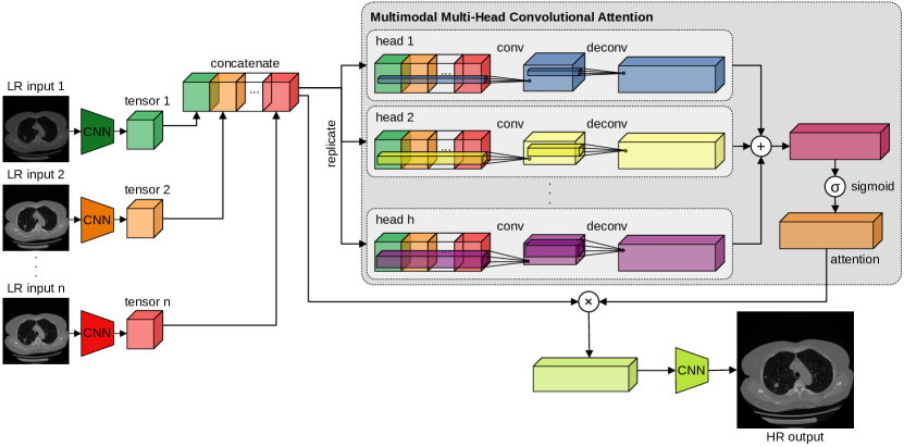
Figure 1: Our multimodal multi-head convolutional attention module (MMHCA) with $h$ heads, integrated into some neural architecture for super-resolution. Input low-resolution (LR) images of distinct contrasts are processed by independent branches and the resulting tensors are concatenated. The concatenated tensor is provided as input to every attention head. Each attention head applies conv and deconv operations, using a kernel size that is unique to the respective head. The resulting tensors are summed up and passed through a sigmoid layer. Finally, the attention tensor is multiplied (element-wise) with the concatenated tensor, and the result is further processed by the network to obtain the high-resolution (HR) image. Best viewed in color.

To approach multi-contrast medical image super-resolution, we propose a novel multimodal multi-head convolutional attention (MMHCA) mechanism that performs joint spatial and channel attention within each head, by stacking a convolutional (conv) layer and a deconvolutional (deconv) layer, as illustrated in Figure 1. Tensors from different contrast neural branches are concatenated along the channel dimension and given as input to our attention module. The convolutional layer reduces the input tensor both spatially and channel-wise. The channel reduction rate is controlled by adjusting the number of convolutional filters, while the spatial reduction rate is controlled by adjusting the size of the kernel (receptive field). The deconv layer brings the output of the convolutional layer back to its original size. We introduce multiple attention heads, each head having a distinct kernel size corresponding to a particular reduction rate for the spatial attention. The tensors from all attention heads are summed up and passed through a sigmoid layer, obtaining the final attention. The attention tensor is multiplied with the input tensor, enabling the neural network to focus on the most interesting regions from each input image. As other attention modules [19, 29, 43], MMHCA relies on the bottleneck principle to force the model in keeping the information that merits attention.

We integrate our multi-input multi-head convolutional attention into two deep neural architectures for super-resolution [14, 26] and conduct experiments on three data sets: IXI, NAMIC Multimodality, and Coltea-Lung-CT-100W. These data sets contain multi-contrast investigations which allow us to evaluate our multimodal framework. Our results show that MMHCA brings significant performance gains for both neural networks on all three data sets. Moreover, our framework outperforms recently introduced attention modules [10, 29, 43], as well as state-of-the-art methods [5, 12, 14, 21, 24, 26, 37, 45, 47, 48, 49, 50]. Aside from evaluating methods via automatic measures, i.e. the peak signal-to-noise ratio (PSNR) and the structural similarity index measure (SSIM), we conduct a subjective evaluation study, asking three physicians to compare the super-resolution results of a state-of-the-art model, before and after adding MMHCA, without disclosing the method producing each image. The least number of votes assigned by a human annotator to MMHCA is $75\%$, suggesting that its performance gains are indeed significant. In addition, we present ablation results indicating that each component involved in our attention module is important.

In summary, our contribution is threefold:

• We are the first to perform medical image super-resolution using a multimodal low-resolution input.

• We propose a novel multimodal multi-head convolutional attention mechanism for multi-contrast medical image SR.

• We present empirical evidence showing that our attention module brings significant performance gains on three multi-contrast data sets.

2 Related Work

2.1 Image Super-Resolution

Most of the recent works [9, 10, 14, 16, 18, 22, 24, 27, 29, 38, 46, 47, 48, 49, 50, 51, 52] addressing the super-resolution task use deep learning methods in order to increase the resolution of images. One of the early studies employing deep convolution neural networks (CNNs) for super-resolution is the work of Kim et al. [24], which introduces the Very Deep Super-Resolution (VDSR) network. The VDSR model consists of $20$ convolutional layers and takes as input the interpolated low-resolution (ILR) image. Different from the work of Kim et al. [24] which relies on ILR images, Shi et al. [38] proposed the efficient sub-pixel convolutional (ESPC) layer, which learns to upscale low-resolution feature maps into the high-resolution output. By eliminating the reliance on ILR images (which have the same height and width as HR images), ESPC is capable of decreasing the running time by a significant margin. After the introduction of the ESPC layer, many researchers [9, 10, 14, 18, 29, 46, 50] adopted this approach in their super-resolution (SR) models.

Super-resolution methods have also shown their benefits in medical imaging. Medical image super-resolution works can be grouped into two categories, where one category is focused on increasing the resolution of individual CT or MRI slices (2D images) [7, 9, 10, 12, 18, 25, 28, 34, 37, 45, 46, 48, 50], while the other is focused on increasing the resolution of entire 3D scans (volumes) [4, 8, 14, 20, 30]. Similar to [7, 9, 10, 12, 18, 25, 28, 34, 37, 45, 46, 48, 50], in this work, we are focusing on increasing the resolution of CT and MRI slices. Gu et al. [16] proposed the MedSRGAN model in order to upsample the resolution of 2D medical images using Generative Adversarial Networks (GANs) [15]. MedSRGAN employs a residual map attention network in the generator to extract useful information from different channels. Gu et al. [16] also used a multi-task loss function comprised of several losses (content loss, adversarial loss and adversarial feature loss) to train the MedSRGAN model. Georgescu et al. [14] proposed a method to increase the resolution of both 2D and 3D medical images. To super-resolve 3D images, Georgescu et al. [14] used two CNNs in a sequential manner, the first CNN increasing the resolution on two axes (height and width) and the second CNN increasing the resolution on the third axis (depth). Their approach can be used to extend any method from 2D SR to 3D SR, including our own.

Most of the related works employ single-contrast super-resolution (SCSR) [7, 9, 14, 18, 25, 28, 34, 37, 45, 46, 48, 50], meaning that they utilize a single-contrast image as input for the upsampling network. There are also some works that approach multi-contrast super-resolution (MCSR) [10, 27, 47, 51, 52] using an HR image from another modality, e.g. a T1-weighted slice, to increase the resolution of the targeted LR modality, e.g. a T2-weighted slice. Zeng et al. [47] proposed a model consisting of two sub-networks to simultaneously perform SCSR and MCSR. The first sub-network performs SCSR, upsampling the target modality, while the second sub-network uses the output of the first sub-network and an HR image from a different modality to further refine the target modality. Feng et al. [10] proposed a multi-stage integration network (MINet) for MCSR. The MINet model uses two input images that are processed in parallel by two independent networks, and their features are fused at each layer to obtain multi-stage feature representations. Similar to Zeng et al. [47], Feng et al. [10] integrated a second HR modality to increase the performance of their model. Different from previous works [10, 27, 47, 51, 52], we do not employ any HR image to guide our model. Instead, we only rely on the low-resolution images pertaining to different modalities. To the best of our knowledge, we are the first to propose an MCSR method based solely on LR medical images as input.

2.2 Attention Mechanism

The attention mechanism is a very hot topic in the computer vision community, having broad applications ranging from mainstream computer vision tasks, such as image classification [43], to more specific tasks, such as natural image SR [29] and medical image SR [10, 48]. Attention mechanisms are integrated into neural networks to direct the attention of the model to the area with relevant information. Hu et al. [19] proposed the squeeze-and-excitation (SE) block to recalibrate the channel responses, thus performing channel-wise attention. In order to further increase the power of the attention mechanism, Woo et al. [43] proposed the Convolutional Block Attention Module (CBAM), which infers attention maps for two separate dimensions, spatial and channel, in a sequential manner. Niu et al. [29] proposed the channel-spatial attention module (CSAM) to boost the performance of natural image SR. CSAM is composed of 3D conv layers, being able to learn the channel and spatial interdependencies of the features. In a similar fashion to Niu et al. [29], Feng et al. [10] employed 3D conv layers to generate attention maps that capture both channel and spatial information. Unlike previous works [10, 29, 43], our attention module is based on 2D convolution and deconvolution operations with multiple kernel sizes to perform joint multi-head spatial-channel attention.

The self-attention mechanism [40] triggered the development of models solely based on attention, such as vision transformers [2, 3, 6, 13, 23, 31, 33, 39, 44, 53, 54], which have been adopted at an astonishing rate by the computer vision and medical imaging communities, likely due to the impressive results across a wide range of problems, from object recognition [6, 39, 44] and object detection [2, 53, 54] to medical image segmentation [3, 13, 17] and medical image generation [33]. Although transformers [36] have been applied to several mainstream medical imaging tasks, the number of transformer-based methods applied to medical image super-resolution is relatively small [11, 12]. Different from methods relying solely on attention-based architectures [11, 12], we propose a novel and flexible attention module that can be integrated into various architectures. To support this claim, we integrate MMHCA into two state-of-the-art architectures [14, 26], providing empirical evidence showing that our attention module can significantly boost the performance of both models.

3 Method

Given a multi-contrast input formed of $n$ low-resolution input images of $p\times p$ pixels, denoted as $LR_{1}$, $LR_{2}$, …, $LR_{n}$, our goal is to obtain an HR image of $r\times r$ pixels, denoted as $HR_{k}$, where $r>p$, for the target modality $k\in\{1,2,...,n\}$. In common practice, $r$ is typically chosen to be equal to $2p$ or $4p$, corresponding to super-resolution factors of $2\times$ or $4\times$, respectively. In our experiments, we consider these commonly-used SR factors.

We propose a spatial-channel attention module to combine the information contained by the multi-contrast LR images. As illustrated in Figure 1, our multimodal multi-head convolutional attention (MMHCA) mechanism can be introduced at any layer of any neural architecture, thus being generic and flexible. We underline that if the baseline architecture is designed for a single-contrast input, we can easily extend the architecture to a multi-contrast input of $n$ contrasts by replicating the neural branch that comes before our module, for a number of $n$ times. Let $f_{i}$ be the neural branch that processes the input $LR_{i}$. We first obtain the encoding tensor $T_{i}$ for each input $LR_{i}$, as follows:

$$T_{i}=f_{i}\left(\theta_{f_{i}},LR_{i}\right),$$ (1)

where $\theta_{f_{i}}$ are the weights of the neural branch $f_{i}$.

The next step in our approach is to concatenate the encoding tensors $T_{i}$ of all modalities along the channel axis, obtaining the tensor $T_{\circ}$, as follows:

$$T_{\circ}=concat\left(T_{1},T_{2},...,T_{n}\right),$$ (2)

where $concat$ represents the concatenation operation. If a multimodal input is not available, our multi-head convolutional attention (MHCA) module can still be applied by considering $T_{\circ}=T_{1}$, where $T_{1}$ is the encoding tensor of the single-contrast input. We use this ablated configuration in our experiments to show the benefits of using multiple modalities as opposed to a single modality.

Next, we apply the multi-head convolutional attention. Our attention module is composed of multiple heads, which are applied on the concatenation of the encoding tensors, denoted as $T_{\circ}$. Each head $h_{j}$, $j\in\{1,2,...,h\}$, where $h$ is the number of heads, is composed of a conv layer followed by a deconv layer, performing both spatial and channel attention. The conv layer jointly reduces the spatial and channel dimensions of the input, while the deconv layer is configured to revert the dimensional reduction performed by the conv layer, thus restoring the size of the output tensor to the size of the input tensor $T_{\circ}$.

For the $j$-th convolutional attention head $h_{j}$, we set the conv kernel size $k_{j}$ to $2\cdot(j-1)+1$. Hence, the first head is formed of kernels having a receptive field of $1\times 1$, the second head is formed of kernels having a receptive field of $3\times 3$, and so on. We note that each kernel size corresponds to a different reduction rate of the spatial attention. For each head $h_{j}$, we set the number of conv filters to $\frac{c}{r}$, where $c$ is the number of input channels and $r$ is the reduction rate of the channel attention. Then, we apply a deconv layer with $c$ filters and the kernel size set to $k_{j}\times k_{j}$ to increase the spatial size of the activation maps. We use a stride of $1$ and a padding equal to $0$ for both conv and deconv layers. In summary, the output $H_{j}$ of the attention head $h_{j}$ is computed as follows:

$$H_{j}=h_{j}\left(\theta_{c_{j}},\theta_{d_{j}},T_{\circ}\right)=max\left(0,T_{\circ}\ast\theta_{c_{j}}\right)\circledast\theta_{d_{j}},$$ (3)

where $\theta_{c_{j}}$ are the learnable weights of the conv layer comprising $\frac{c}{r}$ filters with a kernel size of $k_{j}\times k_{j}$, $\theta_{d_{j}}$ are the parameters of the deconv layer comprising $c$ filters with a kernel size of $k_{j}\times k_{j}$, $max(0,\cdot)$ is the ReLU activation function, $\ast$ is the convolution operation and $\circledast$ is the deconvolution operation. We hereby note that the tensors $H_{1}$, $H_{2}$, …, $H_{h}$ are of the same size.

Next, we sum all the tensors $H_{j}$ produced by the attention heads, obtaining $H_{+}$, as follows:

$$H_{+}=\sum_{j=1}^{h}H_{j}.$$ (4)

We then pass the resulting tensor through the sigmoid function in order to obtain the final attention tensor denoted as $A$, as follows:

$$A=\sigma\left(H_{+}\right).$$ (5)

To apply the learned attention to the encoding tensors, the attention tensor $A$ is multiplied with the tensor $T_{\circ}$, obtaining the tensor $T_{*}$, as follows:

$$T_{*}=T_{\circ}\otimes A,$$ (6)

where $\otimes$ denotes the element-wise multiplication operation.

Let $g$ denote the neural branch that takes $T_{*}$ as input and produces the high-resolution output. The last processing required to obtain the final output of the neural architecture is expressed as follows:

$$HR_{k}=g\left(\theta_{g},T_{*}\right),$$ (7)

where $\theta_{g}$ are the learnable weights of $g$.

4 Experiments

4.1 Data Sets

IXI. The IXI data set is the largest benchmark considered in our evaluation. We use the same version of the IXI data set as [48, 50]. The data set contains 3D multimodal MRI scans, where each MRI has three modalities, namely T1-weighted (T1w), T2-weighted (T2w) and Proton Density (PD). The data set is split into $500$ multimodal MRI scans for training, $6$ multimodal scans for validation and the remaining $70$ multimodal scans for testing. Each MRI scan has $96$ slices with the resolution of $240\times 240$ pixels.

NAMIC Brain Multimodality. The National Alliance for Medical Image Computing (NAMIC) Brain Multimodality data set is formed of $20$ 3D MRI scans. Each 3D image is formed of $176$ slices with the resolution of $256\times 256$ pixels. The data set contains two modalities, namely T1w and T2w. Following [14, 32], we randomly split the data set into $10$ multimodal MRI scans for training and $10$ multimodal MRI scans for testing. We randomly take $2$ MRI scans from the training set to create a validation set for hyperparameter tuning.

Coltea-Lung-CT-100W. The Coltea-Lung-CT-100W data set was recently introduced by Ristea et al. [33]. It contains $100$ triphasic (multimodal) lung CT scans. Each scan has three modalities, namely native, arterial and venous. The entire data set is formed of $12,\!430$ triphasic slices and each slice has $512\times 512$ pixels. The data set is split into $70$ multimodal CT scans for training, $15$ multimodal scans for validation and $15$ multimodal scans for testing.

4.2 Evaluation Metrics

As evaluation metrics, we employ the peak signal-to-noise ratio (PSNR) and the structural similarity index measure (SSIM) [41]. PSNR is the ratio between the maximum possible signal and the power of the noise. It only takes into account the difference between pixels, without quantifying the structural similarity. SSIM [41] takes the structural similarity into account by combining the contrast, the luminance and the texture of the images. Higher values of PSNR and SSIM indicate better reconstruction. We emphasize that PSNR is represented in the log-scale. Hence, seemingly small gains in terms of PSNR can indicate significant quality improvements.

To further assess the improvement brought by our attention module, we also conduct a subjective evaluation study, asking three physicians (specialized in radiology) from the Colţea Hospital to compare the super-resolution results of a state-of-the-art model, before and after adding MMHCA.

4.3 Implementation Details

We compare our attention module with CSAM [10, 29] and CBAM [43]. We consider EDSR [26] and CNN+ESPC [14] as underlying models for the attention mechanisms. To train the EDSR and CNN+ESPC models, we use the official code released by the corresponding authors. For the EDSR [26] network, we set $B=16$ and $F=64$. All the other hyperparameters are left unchanged. For CNN+ESPC [14], we use the same hyperparameters as suggested by the authors.

For a fair comparison, we integrate all the attention modules in the same manner into both networks. For the experiments with single-contrast inputs, we integrate the modules (CSAM, CBAM, MHCA) after each ResBlock. For the experiments with multi-contrast inputs, we replicate the sub-network which ends just before the upsampling layer, creating copies of the sub-network (each copy having its own learnable weights). Then, we concatenate the output of each sub-network and introduce the attention modules (MCSAM, MCBAM, MMHCA). The multi-contrast inputs are used without prior alignment.

For MHCA/MMHCA, we tune the number of heads $h$ and the channel reduction ratio $r$ on the validation set of each benchmark. We find that the optimal configuration is based on $h=3$ heads and a channel reduction ratio of $r=0.5$. This configuration uses kernel sizes of $1\times 1$ for $h_{1}$, $3\times 3$ for $h_{2}$, and $5\times 5$ for $h_{3}$, respectively.

When comparing our attention modules (MHCA/MMHCA) with CSAM/MCSAM [10, 29] and CBAM/MCBAM [43], we use the official code released by the respective authors. As for MHCA/MMHCA, we tune the hyperparameters of CBAM/MCBAM on the validation sets, while CSAM/MCSAM have no hyperparameters that would require tuning. The optimal configuration for CBAM/MCBAM uses a kernel size of $7\times 7$ and a reduction ratio of $0.5$.

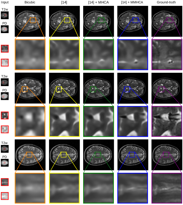
Figure 2: Examples of super-resolved MRI slices from the IXI data set, for an upscaling factor of $4\times$. The HR images produced by two baselines (bicubic interpolation and CNN+ESPC [14]) are compared with the images given by two enhanced versions of CNN+ESPC [14], one based on our single-contrast attention module (MHCA), and another based on our multimodal attention module (MMHCA).

Method	$2\times$	$4\times$
	PSNR/SSIM	PSNR/SSIM
Bicubic	$33.44/0.9589$	$27.86/0.8611$
SRCNN [5]	$37.32/0.9796$	$29.69/0.9052$
VDSR [24]	$38.65/0.9836$	$30.79/0.9240$
IDN [21]	$39.09/0.9846$	$31.37/0.9312$
RDN [49]	$38.75/0.9838$	$31.45/0.9324$
FSCWRN [37]	$39.44/0.9855$	$31.71/0.9359$
CSN [50]	$39.71/0.9863$	$32.05/0.9413$
T2Net [12]	$29.38/0.8720$	$28.66/0.8500$
SERAN [48]	$40.18/0.9872$	$32.40/0.9455$
SERAN+ [48]	${\color[rgb]{0,0,1}40.30}/{\color[rgb]{0,0,1}0.9874}$	${\color[rgb]{0,0,1}32.62}/{\color[rgb]{1,0,0}0.9472}$
EDSR [26]	$39.81/0.9865$	$31.83/0.9377$
EDSR [26] + CSAM [10, 29]	$39.81/0.9865$	$31.83/0.9377$
EDSR [26] + CBAM [43]	$39.82/0.9865$	$31.81/0.9374$
EDSR [26] + MHCA (ours)	$40.11/0.9871$	$32.15/0.9418$
EDSR [26] + MCSAM [10, 29]	$40.12/0.9871$	$32.17/0.9417$
EDSR [26] + MCBAM [43]	$40.13/0.9871$	$32.18/0.9421$
EDSR [26] + MMHCA (ours)	$40.28/{\color[rgb]{0,0,1}0.9874}$	$32.51/0.9452$
EDSR [26] + MMHCA+ (ours)	${\color[rgb]{1,0,0}40.43}/{\color[rgb]{1,0,0}0.9877}$	${\color[rgb]{1,0,0}32.70}/{\color[rgb]{0,0,1}0.9469}$
CNN+ESPC [14]	$38.67/0.9837$	$30.57/0.9210$
CNN+ESPC [14] + CSAM [10, 29]	$38.57/0.9835$	$30.58/0.9211$
CNN+ESPC [14] + CBAM [43]	$38.67/0.9838$	$30.47/0.9192$
CNN+ESPC [14] + MHCA (ours)	$39.04/0.9847$	$30.76/0.9233$
CNN+ESPC [14] + MCSAM [10, 29]	$38.98/0.9845$	$30.94/0.9265$
CNN+ESPC [14] + MCBAM [43]	$38.91/0.9844$	$30.79/0.9238$
CNN+ESPC [14] + MMHCA (ours)	$39.71/0.9862$	$31.52/0.9337$
CNN+ESPC [14] + MMHCA+ (ours)	$39.76/0.9863$	$31.52/0.9337$

Table 1: PSNR and SSIM scores of various state-of-the-art methods [5, 12, 14, 21, 24, 26, 37, 49, 48, 50] on the IXI data set, for the T2w target modality. For two of the existing methods (EDSR [26] and CNN+ESPC [14]), we evaluate enhanced versions, considering various state-of-the-art attention modules [10, 29, 43], as well as our own attention module (MMHCA). We consider both single-contrast (CSAM, CBAM, MHCA) and multi-contrast (MCSAM, MCBAM, MMHCA, MMHCA⁺) versions. The top two scores for each scaling factor ($2\times$ and $4\times$) are highlighted in red and blue, respectively.

Method	$2\times$	$4\times$
	PSNR/SSIM	PSNR/SSIM
Bicubic	$37.61/0.9794$	$31.35/0.9091$
MCSR [47]	$38.32/0.9450$	$30.84/0.8110$
GAN-CIRCLE [45]	$36.19/0.9594$	$-$
EDSR [26]	$41.46/0.9906$	$34.50/0.9558$
EDSR [26] + CSAM [10, 29]	$41.43/0.9905$	$34.53/0.9560$
EDSR [26] + CBAM [43]	$38.66/0.9840$	$32.59/0.9328$
EDSR [26] + MHCA (ours)	$41.94/0.9914$	$34.99/0.9601$
EDSR [26] + MCSAM [10, 29]	$41.52/0.9907$	$34.66/0.9571$
EDSR [26] + MCBAM [43]	$41.49/0.9906$	$34.65/0.9569$
EDSR [26] + MMHCA (ours)	${\color[rgb]{0,0,1}42.15}/{\color[rgb]{0,0,1}0.9917}$	${\color[rgb]{0,0,1}35.35}/{\color[rgb]{0,0,1}0.9624}$
EDSR [26] + MMHCA+ (ours)	${\color[rgb]{1,0,0}42.32}/{\color[rgb]{1,0,0}0.9919}$	${\color[rgb]{1,0,0}35.58}/{\color[rgb]{1,0,0}0.9638}$
CNN+ESPC [14]	$40.73/0.9893$	$33.92/0.9509$
CNN+ESPC [14] + CSAM [10, 29]	$40.46/0.9888$	$33.86/0.9503$
CNN+ESPC [14] + CBAM [43]	$40.54/0.9889$	$33.60/0.9492$
CNN+ESPC [14] + MHCA (ours)	$40.81/0.9894$	$33.94/0.9511$
CNN+ESPC [14] + MCSAM [10, 29]	$40.74/0.9893$	$34.04/0.9518$
CNN+ESPC [14] + MCBAM [43]	$40.73/0.9892$	$33.88/0.9516$
CNN+ESPC [14] + MMHCA (ours)	$41.58/0.9908$	$34.64/0.9573$
CNN+ESPC [14] + MMHCA+ (ours)	$41.49/0.9904$	$34.70/0.9573$

Table 2: PSNR and SSIM scores of various state-of-the-art methods [14, 26, 45, 47] on the NAMIC data set, for the T2w target modality. For two of the existing methods (EDSR [26] and CNN+ESPC [14]), we evaluate enhanced versions, considering various state-of-the-art attention modules [10, 29, 43], as well as our own attention module (MMHCA). We consider both single-contrast (CSAM, CBAM, MHCA) and multi-contrast (MCSAM, MCBAM, MMHCA, MMHCA⁺) versions. The top two scores for each scaling factor ($2\times$ and $4\times$) are highlighted in red and blue, respectively.

Method	$2\times$	$4\times$
	PSNR/SSIM	PSNR/SSIM
Bicubic	$38.84/0.9477$	$31.47/0.8774$
EDSR [26]	$45.11/0.9621$	$39.52/0.9394$
EDSR [26] + CSAM [10, 29]	$45.12/0.9622$	$39.57/0.9395$
EDSR [26] + CBAM [43]	$41.14/0.9538$	$32.92/0.9023$
EDSR [26] + MHCA (ours)	$45.50/0.9634$	${\color[rgb]{1,0,0}40.23}/{\color[rgb]{1,0,0}0.9416}$
EDSR [26] + MCSAM [10, 29]	$45.16/0.9623$	$39.62/0.9397$
EDSR [26] + MCBAM [43]	$45.12/0.9622$	$39.65/0.9397$
EDSR [26] + MMHCA (ours)	${\color[rgb]{0,0,1}45.58}/{\color[rgb]{0,0,1}0.9647}$	$40.06/0.9404$
EDSR [26] + MMHCA+ (ours)	${\color[rgb]{1,0,0}45.68}/{\color[rgb]{1,0,0}0.9649}$	${\color[rgb]{0,0,1}40.22}/{\color[rgb]{0,0,1}0.9409}$
CNN+ESPC [14]	$44.47/0.9599$	$38.34/0.9338$
CNN+ESPC [14] + CSAM [10, 29]	$44.45/0.9599$	$38.36/0.9337$
CNN+ESPC [14] + CBAM [43]	$44.44/0.9601$	$37.23/0.9308$
CNN+ESPC [14] + MHCA (ours)	$44.72/0.9608$	$38.62/0.9348$
CNN+ESPC [14] + MCSAM [10, 29]	$44.51/0.9599$	$38.38/0.9338$
CNN+ESPC [14] + MCBAM [43]	$44.43/0.9600$	$38.19/0.9318$
CNN+ESPC [14] + MMHCA (ours)	$45.05/0.9621$	$38.96/0.9365$
CNN+ESPC [14] + MMHCA+ (ours)	$45.14/0.9623$	$39.10/0.9370$

Table 3: PSNR and SSIM scores of two state-of-the-art methods [14, 26] on the Coltea-Lung-CT-100W data set, for the native target modality. We evaluate enhanced versions of the existing methods, considering various state-of-the-art attention modules [10, 29, 43], as well as our own attention module (MMHCA). We consider both single-contrast (CSAM, CBAM, MHCA) and multi-contrast (MCSAM, MCBAM, MMHCA, MMHCA⁺) versions. The top two scores for each scaling factor ($2\times$ and $4\times$) are highlighted in red and blue, respectively.

Method	EDSR [26]	EDSR [26] + MMHCA (ours)
Doctor $\#1$	$11$	$89$
Doctor $\#2$	$25$	$75$
Doctor $\#3$	$20$	$80$
Average (%)	$18.6\%$	$\mathbf{81.3}\%$

Table 4: Subjective human evaluation results based on 100 randomly selected cases from the IXI test set for EDSR [26], with and without MMHCA, considering an upscaling factor of $4\times$. The reported numbers represent votes awarded by three physicians (with expertise in radiology) for each model.

Method	PSNR/SSIM
EDSR [26]	$41.46/0.9906$
EDSR [26] + MHCA (1 head, r = $0.5$)	$41.40/0.9904$
EDSR [26] + MHCA (2 heads, r = $0.5$)	$41.79/0.9911$
EDSR [26] + MHCA (3 heads, r = $0.5$)	$41.94/0.9914$
EDSR [26] + MHCA (4 heads, r = $0.5$)	$41.90/0.9913$
EDSR [26] + MHCA (3 heads, no deconv, r = $0.5$)	$41.90/0.9913$
EDSR [26] + MHCA (4 heads, $1\!\times\!1$ kernels, r = $2$)	$41.04/0.9898$
EDSR [26] + MHCA (4 heads, r = $2$)	$41.89/0.9913$
EDSR [26] + multimodal input	$41.50/0.9907$
EDSR [26] + MMHCA (1 head, r = $0.5$)	$41.76/0.9911$
EDSR [26] + MMHCA (2 heads, r = $0.5$)	$42.05/0.9915$
EDSR [26] + MMHCA (3 heads, r = $0.5$)	$42.15/0.9917$
EDSR [26] + MMHCA (4 heads, r = $0.5$)	$42.09/0.9916$
EDSR [26] + MMHCA (3 heads, no deconv, r = $0.5$)	$41.87/0.9912$
EDSR [26] + MMHCA (4 heads, $1\!\times\!1$ kernels, r = $2$)	$41.73/0.9910$
EDSR [26] + MMHCA (4 heads, r = $2$)	$42.05/0.9915$

Table 5: Ablation results with EDSR [26] on the NAMIC data set, for a scaling factor of $2\times$ and the T2w target modality. We consider different configurations for MHCA/MMHCA, varying the number of heads, the number of inputs, and the size of kernels.

4.4 Results

Following [10, 27, 47, 51, 52], we conduct experiments on the T2w target modality for the IXI and NAMIC data sets. The ⁺ sign after a method’s name indicates the use of the geometric self-ensemble [26].

IXI. We present the results obtained on the IXI data set for two upscaling factors, $2\times$ and $4\times$, in Table 1. The EDSR [26] model obtains a PSNR of $39.81$ and an SSIM of $0.9865$ for an upscaling factor of $2\times$. When we add the MHCA module to the single-contrast network, the performance increases to $40.11$ and $0.9871$ in terms of PSNR and SSIM, respectively. When we switch to the multimodal input, we observe performance improvements, regardless of the integrated attention module (MCSAM [10, 29], MCBAM [43] or MMHCA). This confirms our hypothesis that the information from the multi-contrast LR images is useful. By adding MMHCA, the performance improves even further, exceeding the performance of both MCSAM and MCBAM. When EDSR is employed as underlying model, MMHCA⁺ brings significant gains, generally outperforming the state-of-the-art methods [5, 12, 14, 21, 24, 26, 37, 48, 49, 50].

In Figure 2, we illustrate qualitative results obtained by two baselines (bicubic and CNN+ESPC [14]) versus two enhanced versions of CNN+ESPC [14], namely CNN+ESPC [14] + MHCA and CNN+ESPC [14] + MMHCA, for an upscaling factor of $4\times$. We observe that our CNN+ESPC [14] + MMHCA model obtains superior SR results compared with the baselines (bicubic, CNN+ESPC [14]), being able to recover structural details that are completely lost by the baselines.

NAMIC. We show the results obtained on the NAMIC data set for two upscaling factors, $2\times$ and $4\times$, in Table 2. The baseline CNN+ESPC [14] obtains a score of $33.92$ in terms of PSNR and $0.9509$ in terms of SSIM, for an upscaling factor of $4\times$. When we add MHCA and MMHCA, the scores improve by considerable margins (in terms of PSNR, the minimum improvement is $0.69$), regardless of the scale ($2\times$ or $4\times$) or the underlying model (EDSR [26] or CNN+ESPC [14]).

Coltea-Lung-CT-100W. We show the results obtained on the Coltea-Lung-CT-100W for two upscaling factors, $2\times$ and $4\times$, in Table 3. Once again, we observe performance improvements brought by the use of multi-contrast LR inputs, the only attention that does not increase the baseline performance being MCBAM [43]. Our MMHCA module exceeds the baseline and the other attention modules by significant margins (in terms of PSNR, the minimum improvement is $0.47$), regardless of the scale or the network.

Quality assessment by physicians. In Table 4, we present the results of our subjective human evaluation study based on 100 cases, which are randomly selected from the IXI test set, for EDSR [26], with and without MMHCA, considering an upscaling factor of $4\times$. The quality evaluation study was completed by three physicians with expertise in radiology. The doctors had to choose between two images (randomly positioned on the left side or right side of the ground-truth HR image), without knowing which method produced each image. The HR images obtained after adding MMHCA were chosen in a proportion of $81.3\%$ against the images produced by the baseline EDSR [26]. Upon disclosing the method producing each image, the doctors concluded that MMHCA helps to recover important details, e.g. blood vessels, which are missed by the baseline EDSR.

Ablation study. In Table 5, we present an ablation study on the NAMIC data set for a scaling factor of $2\times$. We observe that the best performance is obtained when the number of heads is equal to $3$, regardless of the number of input modalities (MHCA or MMHCA). We also notice that every configuration of our MMHCA module obtains better results than the concatenation of the features without any attention (multimodal input). To demonstrate the utility of the bottleneck principle, we test an ablated version of MHCA and MMHCA based on 3 heads, that does not reduce the input tensor through convolution, hence removing the deconv layer. This ablated version (3 heads, no deconv) attains lower performance compared to the complete version of MHCA and MMHCA based on 3 heads. This experiment supports our design based on the bottleneck principle through the conv and deconv operations. To show that the diversity of the heads is important, we compare two modules with $4$ heads each and a reduction ratio of $r=2$, one where all kernel sizes are $1\times 1$, and another where the kernels are of different sizes, from $1\times 1$ to $7\times 7$. The module based on diverse heads leads to significantly better results, indicating that using the same kernel size for all heads is suboptimal. In terms of the number of parameters, the module with 4 heads, $r=2$ and kernels of $1\times 1$ is equivalent to the module with 1 head and $r=0.5$. The module with 1 head attains superior results, showing that simply adding more heads of the same kind is not useful. In summary, the empirical results show that our method obtains superior results not because of the increased capacity of the model, but due to the diversity of the heads.

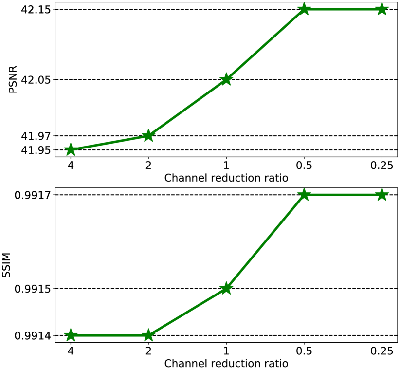
Figure 3: PSNR and SSIM scores of the EDSR [26] + MMHCA method, considering channel reduction rates in the set $\{4,2,1,0.5,0.25\}$. Results are reported on the NAMIC data set for an upscaling factor of $2\times$.

In Figure 3, we illustrate the impact of the channel reduction ratio on the MMHCA module based on 3 heads. We observe that the performance increases with the ratio until $r=0.5$. After this point, further increasing the ratio does not improve performance.

5 Conclusion

In this paper, we presented a novel multimodal multi-head convolutional attention (MMHCA) module, which performs joint spatial and channel attention. We integrated our module into two neural networks [14, 26] and conducted experiments on three multimodal medical image benchmarks: IXI, NAMIC and Coltea-Lung-CT-100W. We showed that our attention module yields higher gains compared with competing attention modules [10, 29, 43], being able to bring the performance of the underlying models above the state-of-the-art results [5, 12, 14, 21, 24, 26, 37, 45, 47, 48, 49, 50].

In future work, we aim to integrate our module into further neural models and extend its applicability to natural images. We will also study the utility of the SR results in better solving other tasks, e.g. medical image segmentation.

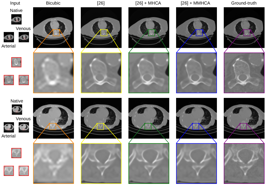
Figure 4: Examples of super-resolved CT images from the Coltea-Lung-CT-100W data set, for an upscaling factor of $4\times$. The HR images produced by two baselines (bicubic interpolation and EDSR [26]) are compared with the images given by two enhanced versions of EDSR [26], one based on our single-contrast attention module (MHCA), and another based on our multimodal attention module (MMHCA).

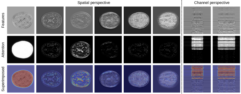
Figure 5: Views (top row) of a tensor computed for an example from NAMIC, which is given as input to MMHCA, and the corresponding attention maps (middle row) along the spatial (first six columns) and channel (last two columns) dimensions, showing that MMHCA performs joint channel and spatial attention. Views with superimposed attention maps are displayed on the bottom row. Best viewed in color.

6 Supplementary

6.1 Additional Qualitative Results

In Figure 4, we illustrate qualitative results obtained by two baselines (bicubic and EDSR [26]) versus two enhanced versions of EDSR [26], namely EDSR [26] + MHCA and EDSR [26] + MMHCA, for an upscaling factor of $4\times$. We observe that our EDSR [26] + MMHCA model is able to create sharper reconstructions and to improve the contrast levels.

6.2 Attention Visualization

In Figure 5, we show various perspectives along the spatial and channel dimensions of a tensor given as input to MMHCA. Looking at the attention corresponding to individual activation maps (first six columns), we observe that our module attends to salient contours and edges, or even full organs. Analyzing the attention along the channel axis (last two columns), we observe that, in this example, our module tends to mainly focus on the first LR input, naturally because the first LR input is the modality (contrast type) that corresponds to the HR output, containing the most relevant information to super-resolve the image. In contrast, the second modality is scarcely attended by our module. Overall, we observe that MMHCA performs both spatial and channel attention, confirming that our attention module works as intended.

References

- [1] Mihail Burduja, Radu Tudor Ionescu, and Nicolae Verga. Accurate and efficient intracranial hemorrhage detection and subtype classification in 3D CT scans with convolutional and long short-term memory neural networks. Sensors, 20(19):5611, 2020.
- [2] Nicolas Carion, Francisco Massa, Gabriel Synnaeve, Nicolas Usunier, Alexander Kirillov, and Sergey Zagoruyko. End-to-end object detection with transformers. In Proceedings of ECCV, pages 213–229, 2020.
- [3] Jieneng Chen, Yongyi Lu, Qihang Yu, Xiangde Luo, Ehsan Adeli, Yan Wang, Le Lu, Alan L Yuille, and Yuyin Zhou. TransUNet: Transformers Make Strong Encoders for Medical Image Segmentation. arXiv preprint arXiv:2102.04306, 2021.
- [4] Yuhua Chen, Feng Shi, Anthony G Christodoulou, Yibin Xie, Zhengwei Zhou, and Debiao Li. Efficient and accurate MRI super-resolution using a generative adversarial network and 3D multi-level densely connected network. In Proceedings of MICCAI, pages 91–99, 2018.
- [5] Chao Dong, Chen Change Loy, Kaiming He, and Xiaoou Tang. Image super-resolution using deep convolutional networks. IEEE Transactions on Pattern Analysis and Machine Intelligence, 38(2):295–307, 2016.
- [6] Alexey Dosovitskiy, Lucas Beyer, Alexander Kolesnikov, Dirk Weissenborn, Xiaohua Zhai, Thomas Unterthiner, Mostafa Dehghani, Matthias Minderer, Georg Heigold, Sylvain Gelly, et al. An image is worth 16x16 words: Transformers for image recognition at scale. In Proceedings of ICLR, 2021.
- [7] Jinglong Du, Zhongshi He, Lulu Wang, Ali Gholipour, Zexun Zhou, Dingding Chen, and Yuanyuan Jia. Super-resolution reconstruction of single anisotropic 3D MR images using residual convolutional neural network. Neurocomputing, 392:209–220, 2020.
- [8] Jinglong Du, Lulu Wang, Ali Gholipour, Zhongshi He, and Yuanyuan Jia. Accelerated Super-resolution MR Image Reconstruction via a 3D Densely Connected Deep Convolutional Neural Network. In Proceedings of BIBM, pages 349–355, 2018.
- [9] Xiaofeng Du and Yifan He. Gradient-Guided Convolutional Neural Network for MRI Image Super-Resolution. Applied Sciences, 9(22):4874, 2019.
- [10] Chun-Mei Feng, Huazhu Fu, Shuhao Yuan, and Yong Xu. Multi-Contrast MRI Super-Resolution via a Multi-Stage Integration Network. In Proceedings of MICCAI, pages 140–149, 2021.
- [11] Chun-Mei Feng, Yunlu Yan, Geng Chen, Huazhu Fu, Yong Xu, and Ling Shao. Accelerated Multi-Modal MR Imaging with Transformers. arXiv preprint arXiv:2106.14248, 2021.
- [12] Chun-Mei Feng, Yunlu Yan, Huazhu Fu, Li Chen, and Yong Xu. Task Transformer Network for Joint MRI Reconstruction and Super-Resolution. In Proceedings of MICCAI, pages 307–317, 2021.
- [13] Yunhe Gao, Mu Zhou, and Dimitris Metaxas. UTNet: A Hybrid Transformer Architecture for Medical Image Segmentation. In Proceedings of MICCAI, pages 61–71, 2021.
- [14] Mariana-Iuliana Georgescu, Radu Tudor Ionescu, and Nicolae Verga. Convolutional Neural Networks With Intermediate Loss for 3D Super-Resolution of CT and MRI Scans. IEEE Access, 8:49112–49124, 2020.
- [15] Ian Goodfellow, Jean Pouget-Abadie, Mehdi Mirza, Bing Xu, David Warde-Farley, Sherjil Ozair, Aaron Courville, and Yoshua Bengio. Generative adversarial nets. In Proceedings of NIPS, pages 2672–2680, 2014.
- [16] Yuchong Gu, Zitao Zeng, Haibin Chen, Jun Wei, Yaqin Zhang, Binghui Chen, Yingqin Li, Yujuan Qin, Qing Xie, Zhuoren Jiang, and Yao Lu. Medsrgan: Medical images super-resolution using generative adversarial networks. Multimedia Tools Application, 79(29–30):21815–21840, 2020.
- [17] Ali Hatamizadeh, Dong Yang, Holger Roth, and Daguang Xu. UNETR: Transformers for 3D Medical Image Segmentation. In Proceedings of WACV, pages 574–584, 2022.
- [18] Janka Hatvani, András Horváth, Jérôme Michetti, Adrian Basarab, Denis Kouamé, and Miklós Gyöngy. Deep learning-based super-resolution applied to dental computed tomography. IEEE Transactions on Radiation and Plasma Medical Sciences, 3(2):120–128, 2018.
- [19] Jie Hu, Li Shen, and Gang Sun. Squeeze-and-excitation networks. In Proceedings of CVPR, pages 7132–7141, 2018.
- [20] Y. Huang, L. Shao, and A. F. Frangi. Simultaneous Super-Resolution and Cross-Modality Synthesis of 3D Medical Images Using Weakly-Supervised Joint Convolutional Sparse Coding. In Proceedings of CVPR, pages 5787–5796, 2017.
- [21] Zheng Hui, Xiumei Wang, and Xinbo Gao. Fast and accurate single image super-resolution via information distillation network. In Proceedings of CVPR, pages 723–731, 2018.
- [22] Michal Kawulok, Pawel Benecki, Szymon Piechaczek, Krzysztof Hrynczenko, Daniel Kostrzewa, and Jakub Nalepa. Deep Learning for Multiple-Image Super-Resolution. IEEE Geoscience and Remote Sensing Letters, 17(6):1062–1066, 2020.
- [23] Salman Khan, Muzammal Naseer, Munawar Hayat, Syed Waqas Zamir, Fahad Shahbaz Khan, and Mubarak Shah. Transformers in Vision: A Survey. ACM Computing Surveys, 2021.
- [24] Jiwon Kim, Jung Kwon Lee, and Kyoung Mu Lee. Accurate image super-resolution using very deep convolutional networks. In Proceedings of CVPR, pages 1646–1654, 2016.
- [25] Yinghua Li, Bin Song, Jie Guo, Xiaojiang Du, and Mohsen Guizani. Super-Resolution of Brain MRI Images Using Overcomplete Dictionaries and Nonlocal Similarity. IEEE Access, 7:25897–25907, 2019.
- [26] Bee Lim, Sanghyun Son, Heewon Kim, Seungjun Nah, and Kyoung Mu Lee. Enhanced deep residual networks for single image super-resolution. In Proceedings of CVPR Workshops, pages 136–144, 2017.
- [27] Qing Lyu, Hongming Shan, Cole R. Steber, Corbin A. Helis, Chris Whitlow, Michael Chan, and Ge Wang. Multi-Contrast Super-Resolution MRI Through a Progressive Network. IEEE Transactions on Medical Imaging, 39:2738–2749, 2020.
- [28] Dwarikanath Mahapatra, Behzad Bozorgtabar, and Rahil Garnavi. Image super-resolution using progressive generative adversarial networks for medical image analysis. Computerized Medical Imaging and Graphics, 71:30–39, 2019.
- [29] Ben Niu, Weilei Wen, Wenqi Ren, Xiangde Zhang, Lianping Yang, Shuzhen Wang, Kaihao Zhang, Xiaochun Cao, and Haifeng Shen. Single Image Super-Resolution via a Holistic Attention Network. In Proceedings of ECCV, pages 191–207, 2020.
- [30] Ozan Oktay, Wenjia Bai, Matthew Lee, Ricardo Guerrero, Konstantinos Kamnitsas, Jose Caballero, Antonio de Marvao, Stuart Cook, Declan O’Regan, and Daniel Rueckert. Multi-input Cardiac Image Super-Resolution Using Convolutional Neural Networks. In Proceedings of MICCAI, pages 246–254, 2016.
- [31] Niki Parmar, Ashish Vaswani, Jakob Uszkoreit, Lukasz Kaiser, Noam Shazeer, Alexander Ku, and Dustin Tran. Image transformer. In Proceedings of ICML, pages 4055–4064, 2018.
- [32] Chi-Hieu Pham, Carlos Tor-Díez, Hélène Meunier, Nathalie Bednarek, Ronan Fablet, Nicolas Passat, and François Rousseau. Multiscale brain MRI super-resolution using deep 3D convolutional networks. Computerized Medical Imaging and Graphics, 77:101647, 2019.
- [33] Nicolae-Catalin Ristea, Andreea-Iuliana Miron, Olivian Savencu, Mariana-Iuliana Georgescu, Nicolae Verga, Fahad Shahbaz Khan, and Radu Tudor Ionescu. CyTran: Cycle-Consistent Transformers for Non-Contrast to Contrast CT Translation. arXiv preprint arXiv:2110.06400, 2021.
- [34] Eser Sert, Fatih Özyurt, and Akif Doğantekin. A new approach for brain tumor diagnosis system: single image super resolution based maximum fuzzy entropy segmentation and convolutional neural network. Medical Hypotheses, 133:109413, 2019.
- [35] P. Mohamed Shakeel, M.A. Burhanuddin, and Mohamad Ishak Desa. Lung cancer detection from CT image using improved profuse clustering and deep learning instantaneously trained neural networks. Measurement, 145:702–712, 2019.
- [36] Fahad Shamshad, Salman Khan, Syed Waqas Zamir, Muhammad Haris Khan, Munawar Hayat, Fahad Shahbaz Khan, and Huazhu Fu. Transformers in medical imaging: A survey. arXiv preprint arXiv:2201.09873, 2022.
- [37] Jun Shi, Zheng Li, Shihui Ying, Chaofeng Wang, Qingping Liu, Qi Zhang, and Pingkun Yan. MR Image Super-Resolution via Wide Residual Networks With Fixed Skip Connection. IEEE Journal of Biomedical and Health Informatics, 23(3):1129–1140, 2019.
- [38] Wenzhe Shi, Jose Caballero, Ferenc Huszár, Johannes Totz, Andrew P. Aitken, Rob Bishop, Daniel Rueckert, and Zehan Wang. Real-time single image and video super-resolution using an efficient sub-pixel convolutional neural network. In Proceedings of CVPR, pages 1874–1883, 2016.
- [39] Hugo Touvron, Matthieu Cord, Matthijs Douze, Francisco Massa, Alexandre Sablayrolles, and Hervé Jégou. Training data-efficient image transformers & distillation through attention. In Proceedings of ICML, pages 10347–10357, 2021.
- [40] Ashish Vaswani, Noam Shazeer, Niki Parmar, Jakob Uszkoreit, Llion Jones, Aidan N Gomez, Łukasz Kaiser, and Illia Polosukhin. Attention is all you need. In Proceedings of NIPS, pages 5998–6008, 2017.
- [41] Zhou Wang, Alan C. Bovik, Hamid R. Sheikh, and Eero P. Simoncelli. Image quality assessment: from error visibility to structural similarity. IEEE Transactions on Image Processing, 13(4):600–612, 2004.
- [42] Zhiwei Wang, Chaoyue Liu, Xiang Bai, and Xin Yang. DeepCADx: Automated Prostate Cancer Detection and Diagnosis in mp-MRI Based on Multimodal Convolutional Neural Networks. In Proceedings of ACMMM, pages 1229––1230, 2017.
- [43] Sanghyun Woo, Jongchan Park, Joon-Young Lee, and In-So Kweon. CBAM: Convolutional Block Attention Module. In Proceedings of ECCV, pages 3–19, 2018.
- [44] Haiping Wu, Bin Xiao, Noel Codella, Mengchen Liu, Xiyang Dai, Lu Yuan, and Lei Zhang. CvT: Introducing Convolutions to Vision Transformers. In Proceedings of ICCV, pages 22–31, 2021.
- [45] Chenyu You, Guang Li, Yi Zhang, Xiaoliu Zhang, Hongming Shan, Mengzhou Li, Shenghong Ju, Zhen Zhao, Zhuiyang Zhang, Wenxiang Cong, et al. CT super-resolution GAN constrained by the identical, residual, and cycle learning ensemble (GAN-CIRCLE). IEEE Transactions on Medical Imaging, 39:188–203, 2020.
- [46] Haichao Yu, Ding Liu, Honghui Shi, Hanchao Yu, Zhangyang Wang, Xinchao Wang, Brent Cross, Matthew Bramler, and Thomas S Huang. Computed tomography super-resolution using convolutional neural networks. In Proceedings of ICIP, pages 3944–3948, 2017.
- [47] Kun Zeng, Hong Zheng, Congbo Cai, Yu Yang, Kaihua Zhang, and Zhong Chen. Simultaneous single- and multi-contrast super-resolution for brain MRI images based on a convolutional neural network. Computers in Biology and Medicine, 99:133–141, 2018.
- [48] Yulun Zhang, Kai Li, Kunpeng Li, and Yun Fu. MR Image Super-Resolution with Squeeze and Excitation Reasoning Attention Network. In Proceedings of CVPR, pages 13420–13429, 2021.
- [49] Yulun Zhang, Yapeng Tian, Yu Kong, Bineng Zhong, and Yun Fu. Residual dense network for image super-resolution. In Proceedings of CVPR, pages 2472–2481, 2018.
- [50] Xiaole Zhao, Yulun Zhang, Tao Zhang, and Xueming Zou. Channel Splitting Network for Single MR Image Super-Resolution. IEEE Transactions on Image Processing, 28(11):5649–5662, 2019.
- [51] Hong Zheng, Xiaobo Qu, Zhengjian Bai, Yunsong Liu, Di Guo, Jiyang Dong, Xi Peng, and Zhong Chen. Multi-contrast brain magnetic resonance image super-resolution using the local weight similarity. BMC Medical Imaging, 17, 2017.
- [52] Hong Zheng, Kun Zeng, Di Guo, Jiaxi Ying, Yu Yang, Xi Peng, Feng Huang, Zhong Chen, and Xiaobo Qu. Multi-Contrast Brain MRI Image Super-Resolution With Gradient-Guided Edge Enhancement. IEEE Access, 6:57856–57867, 2018.
- [53] Minghang Zheng, Peng Gao, Xiaogang Wang, Hongsheng Li, and Hao Dong. End-to-end object detection with adaptive clustering transformer. In Proceedings of BMVC, 2020.
- [54] Xizhou Zhu, Weijie Su, Lewei Lu, Bin Li, Xiaogang Wang, and Jifeng Dai. Deformable DETR: Deformable Transformers for End-to-End Object Detection. In Proceedings of ICLR, 2020.