Accessing strongly-coupled systems without compromising them

Abstract

The last decades have seen a burst of experimental platforms reaching the so-called strong-coupling regime, where quantum coherent effects dominate over incoherent processes such as dissipation and thermalization. This has allowed us to create highly nontrivial quantum states and put counterintuitive quantum-mechanical effects to test beyond the wildest expectations of the founding fathers of quantum physics. The strong-coupling regime comes with certain challenges though: the need for a large isolation makes it difficult to access the system for control or monitoring purposes. In this work we propose a way to access such systems through an engineered environment that does not compromise their strong-coupling effects. As a proof of principle, we apply the approach to the photon-blockade effect present in nonlinear resonators, but argue that the mechanism is quite universal. We also propose an architecture based on superconducting circuits where the required unconventional environment can be implemented, opening the way to the experimental analysis of our ideas.

Introduction.—The precise control of light-matter interactions is arguably the landmark of quantum optical systems. It has allowed us to handcraft quantum superposition states able to test the laws of quantum mechanics well beyond what the founding fathers of quantum mechanics ever thought possible. The generation of such states is only possible by accessing the so-called strong-coupling regime, meaning that the quantum-coherent part of the evolution induced by the interaction between light and matter (governed by the Schrödinger equation) occurs within a time scale where dissipation and other mechanisms responsible for decoherence are still not relevant. Hence, since the pioneering experiments in cavity quantum electrodynamics (Raimond et al., 2001; Miller et al., 2005; Walther et al., 2006) and trapped ions (Leibfried et al., 2003; Schneider et al., 2012), people have worked hard to achieve the strong-coupling regime in many other platforms, including cold atoms (Jaksch and Zoller, 2005; Bloch et al., 2008), superconducting circuits (Devoret and Schoelkopf, 2013; Blais et al., 2021), and mechanical devices (Aspelmeyer et al., 2014) among others.

Naturally, two strategies can be followed to achieve the strong-coupling regime: enhancing the interactions or decreasing the decoherence rates. One can try to enhance the light-matter interaction by confining the system to smaller volumes or by finding matter with larger dipole moments, but these are features that are not readily available in most experimental platforms. The second route consists in isolating the system incredibly well, but this comes at a high price: it becomes then difficult to access it without compromising its strong coupling, that is, to manipulate it and use its radiating fields for applications.

In this Letter we introduce a way to overcome this last limitation, that is, of connecting the system to an environment that we can use for driving and monitoring purposes, without compromising its strong-coupling regime. Instead of a single environment, our idea uses two environments, and an additional system (twin to the main one, but not necessarily in the strong-coupling regime) that couples to these two environments as well. When the systems couple symmetrically to the environments, a perfectly isolated dark mode appears (Lalumière et al., 2013), which inherits the interactions of the system under the right conditions. By allowing for a slightly asymmetric coupling to the environments, this mode acquires a small coupling into our controlled environment, but effectively remaining in the strong-coupling regime. This mechanism is universal, that is, works for any type of interaction. In order to study it in detail, we consider the case of a nonlinear or Kerr resonator (Imamoglu et al., 1997) and study the so-called photon blockade effect, characteristic of the strong-coupling regime: from a weak input coherent drive, we show that our mechanism indeed leads to strong photon anti-bunching, while keeping large transmission probabilities, and propose a specific architecture based on superconducting circuits where our ideas can be explored.

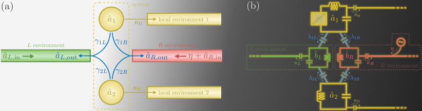
Figure 1: (Color online) (a) Sketch of our system, formed by two bosonic modes $\{\hat{a}_{j}\}_{j=1,2}$, one of them presenting a nonlinearity that is strong with respect to its local decay $\kappa_{0}$, but weak with respect to the coupling to the $L$ and $R$ environments that we use as input/output channels. The excitations of the bosonic modes decay collectively to these two environments through outputs $\{\hat{a}_{\alpha,\text{out}}\propto\sqrt{\gamma_{1\alpha}}\hat{a}_{1}+\sqrt{\gamma_{2\alpha}}\hat{a}_{2}\}_{\alpha=R,L}$, while the environments are driven by input vacuum fluctuations $\{\hat{a}_{\alpha,\text{in}}\}_{\alpha=R,L}$ plus a coherent drive of irradiance $\eta^{2}$ for one environment. As we explain in the text, an asymmetric decay of the modes into the environments ($\gamma_{2R}\approx\gamma_{2L}\gg\gamma_{1R}=\gamma_{1L}$) allows the system to reach an effective strong-coupling regime, as evidenced by strong and robust anti-bunching of the output. (b) Sketch of the experimental proposal. Two LC superconducting circuits (one including some nonlinear element) form the main system, and exchange excitations at rates $\lambda_{j\alpha}$ with two auxiliary LC circuits with corresponding operators $\{\hat{b}_{\alpha}\}_{\alpha=R,L}$, which in turn decay to two transmission lines at rates $\kappa_{\alpha}\gg\lambda_{j\alpha}$. The same idea can be implemented in the optical domain, for example by replacing the LC circuits with whispering gallery mode resonators or photonic crystal cavities, and the transmission lines by photonic fibers.

Note that our mechanism is completely different from the so-called unconventional photon blockade effect (Liew and Savona, 2010; Bamba et al., 2011; Flayac et al., 2015; Flayac and Savona, 2016), which allows generating anti-bunched photon statistics even within the weak-coupling regime by exploiting the coherent tunneling of quanta within two resonators, but requires fine-tuning of the nonlinearity.

Model.—We consider the open quantum system sketched in Fig. 1(a), consisting of two bosonic modes described by annihilation operators $\{\hat{a}_{j}\}_{j=1,2}$ obeying canonical commutation relations $[\hat{a}_{j},\hat{a}_{l}^{\dagger}]=\delta_{jl}$ and $[\hat{a}_{j},\hat{a}_{l}]=0$. Each mode couples to their local environments (inaccessible to the experiment), which induce damping at rates $\kappa_{0}$. In addition, the system couples to two experimentally accessible environments denoted by $L$ and $R$ via the collective jump operators $\{\hat{J}_{\alpha}=\sqrt{\gamma_{1\alpha}}\hat{a}_{1}+\sqrt{\gamma_{2\alpha}}\hat{a}_{2}\}_{\alpha=R,L}$. Hence, rather than considering only independent decay channels for each bosonic mode, we consider a collective coherent decay that will allow us to exploit quantum interference effects, especially when allowing the four decay rates $\gamma_{j\alpha}$ to be independently tunable. We later put forward concrete architectures based on currently available superconducting-circuit technologies where our ideas should be readily implementable, see Fig. 1(b).

Under standard Born-Markov conditions (Gardiner and Zoller, 2004; de Vega and Alonso, 2017; Navarrete-Benlloch, 2022), the fields coming out of the system into the collective environments are characterized by output operators

$$\hat{a}_{\alpha,\mathrm{out}}(t)=\eta\delta_{\alpha,R}+\hat{a}_{\alpha,\mathrm{in}}(t)-\sqrt{2}\mathrm{i}\hat{J}_{\alpha}(t),$$ (1)

where we have assumed that the system is driven from the $R$ environment with flux $\eta^{2}$ (quanta per unit time), and $\hat{a}_{\alpha,\mathrm{in}}(t)$ annihilates the vacuum state of the environmental modes. Both the input and output operators satisfy canonical commutation relations in time, e.g. $[\hat{a}_{\alpha,\mathrm{in}}(t),\hat{a}_{\alpha^{\prime},\mathrm{in}}^{\dagger}(t^{\prime})]=\delta_{\alpha\alpha^{\prime}}\delta(t-t^{\prime})$ and $[\hat{a}_{\alpha,\mathrm{in}}(t),\hat{a}_{\alpha^{\prime},\mathrm{in}}(t^{\prime})]=0$. We work in a picture rotating at the driving frequency, so the operators in this expression are slowly-varying operators, not Heisenberg-picture ones.

For the internal dynamics of the system, we consider linear modes (harmonic oscillators) of the same frequency, one of them containing a weak anharmonicity or Kerr nonlinearity (later we comment on other types of nonlinearity). Again under Born-Markov conditions (Gardiner and Zoller, 2004; de Vega and Alonso, 2017; Navarrete-Benlloch, 2022) and working in a picture rotating at the driving frequency, the evolution of the state of the system $\hat{\rho}$ is governed by the master equation

$$\partial_{t}\hat{\rho}=-\mathrm{i}\left[\hat{H},\hat{\rho}\right]+\sum_{\alpha=L,R}\mathcal{D}_{J_{\alpha}}[\hat{\rho}]+\sum_{j=1}^{2}\kappa_{0}\mathcal{D}_{a_{j}}[\hat{\rho}],$$ (2)

where we have defined the Lindblad dissipator

$$\mathcal{D}_{J}[\hat{\rho}]=2\hat{J}\hat{\rho}\hat{J}^{\dagger}-\hat{J}^{\dagger}\hat{J}\hat{\rho}-\hat{\rho}\hat{J}^{\dagger}\hat{J},$$ (3)

and the Hamiltonian (divided by $\hbar$) reads

$$\hat{H}=\Delta(\hat{a}_{1}^{\dagger}\hat{a}_{1}+\hat{a}_{2}^{\dagger}\hat{a}_{2})+g\hat{a}_{1}^{\dagger 2}\hat{a}_{1}^{2}+\sqrt{2}\eta(\hat{J}_{R}+\hat{J}_{R}^{\dagger}),$$ (4)

being $\Delta$ the detuning between the drive and the oscillators’ frequency.

We consider the situation in which strong coupling has been achieved with respect to the local dissipative channels, while the coupling remains weak with respect to the engineered environments used as input/output channels, that is, $\kappa_{0}<g\ll\gamma_{j\alpha}$. In this work we show how the nonlinear effects that are characteristic of the strong-coupling regime can still be observed by exploiting quantum interference effects coming from the collective character of the jump operators $\hat{J}_{\alpha}$, allowing us to access the system without compromising its strong-coupling regime.

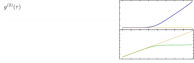
Figure 2: (Color online) (a) Second-order correlation function $g^{(2)}(\tau)$ as a function of the normalized time delay $\Gamma_{-}\tau$ for different values of the normalized input photon flux $N_{\eta}=2\Gamma_{-R}\eta^{2}/\Gamma_{-}^{2}$. Strong anti-bunching is appreciated, even when $N_{\eta}>1$, where our analytical results based on scattering theory (dotted yellow line) cease to apply. (b) characterizes the anti-bunching as a function of $N_{\eta}$, showing $g^{(2)}(0)$ in solid blue, the normalized output photon flux $\bar{n}_{\text{out}}/\Gamma_{-}$ in dashed green, and in dashed-dotted green the normalized time-delay $\Gamma_{-}\tilde{\tau}$ that it takes for the second-order correlation function to grow up to $g^{(2)}(\tilde{\tau})=1/e$, providing a measure for the anti-bunching time-scale. The dotted yellow curves are the analytic results obtained from scattering theory. Note that on the upper panel the left ticks refer to $g^{(2)}(0)$ while the right ones to $\Gamma_{-}\tilde{\tau}$. In all plots we have chosen $y=0.01$, $g=4\times 10^{-4}\gamma_{2}$, $x=0.02\sqrt{g/\gamma_{1}}=0.004$, and $\kappa_{0}=0$.

Intuitive picture.—In order to understand the essence of the mechanism, it is best to consider the $\kappa_{0}=0$ case, and perform a canonical transformation to the basis of modes that diagonalize the dissipative part of the master equation:

$$\hat{A}_{+} =\hat{a}_{1}\cos\theta+\hat{a}_{2}\sin\theta,$$ (5a)

$$\hat{A}_{-} =\hat{a}_{1}\sin\theta-\hat{a}_{2}\cos\theta,$$ (5b)

with $\theta=\arctan[2\gamma_{12}/(\gamma_{1}-\gamma_{2}+\sqrt{(\gamma_{1}-\gamma_{2})^{2}+4\gamma_{12}^{2}})]\in[0,\pi/2]$, where $\gamma_{j}=\gamma_{jR}+\gamma_{jL}$ and $\gamma_{12}=\sqrt{\gamma_{1R}\gamma_{2R}}+\sqrt{\gamma_{1L}\gamma_{2L}}$. In terms of these new ‘normal’ modes, which obey canonical commutation relations unlike the jump operators $\hat{J}_{\alpha}$, the dissipative part of (2) takes the form

$$\sum_{\alpha=L,R}\mathcal{D}_{J_{\alpha}}[\hat{\rho}]=\sum_{n=\pm}\Gamma_{n}\mathcal{D}_{A_{n}}[\hat{\rho}],$$ (6)

with normal damping rates $2\Gamma_{\pm}=\gamma_{1}+\gamma_{2}\pm\sqrt{(\gamma_{1}-\gamma_{2})^{2}+4\gamma_{12}^{2}}.$

Interestingly, when $\gamma_{jR}=\gamma_{jL}$ (that is, when the modes couple in the same way to both environments), mode $\hat{A}_{+}$ gathers all the damping, $\Gamma_{+}=\gamma_{1}+\gamma_{2}$, while mode $\hat{A}_{-}$ effectively becomes dark or undamped, $\Gamma_{-}=0$. If, in addition, we work in the $\gamma_{2}\gg\gamma_{1}$ regime, $\theta\approx\pi/2$, and the nonlinear term $g\hat{a}_{1}^{\dagger 2}\hat{a}_{1}^{2}$ is dominated by the $g_{-}\hat{A}_{-}^{\dagger 2}\hat{A}_{-}^{2}$ contribution, with $g_{-}=g\sin^{4}\theta$. Hence, while mode $\hat{A}_{+}$ is still in the weak-coupling regime, $\Gamma_{+}\gg g$, this is not the case for mode $\hat{A}_{-}$, which in this extreme limit behaves as a dissipativeless anharmonic or nonlinear oscillator.

This provides the intuition that by working close to this regime, specifically keeping $y\equiv\gamma_{1}/\gamma_{2}\ll 1$, but allowing for a slightly asymmetric coupling of the modes to the environments, mode $\hat{A}_{-}$ will effectively enter the strong-coupling regime with $g_{-}\gg\Gamma_{-}$. Specifically, in the following we keep mode-1’s couplings symmetric for simplicity, $\gamma_{1R}=\gamma_{1L}=\gamma_{1}/2$, and define the asymmetry parameter $x\equiv(\gamma_{2R}-\gamma_{2L})/\gamma_{2}$ for the second mode, with $|x|\ll 1$. To the leading orders in $x$ and $y$, the $g_{-}\gg\Gamma_{-}$ condition can be recasted as $|x|\ll 2\sqrt{g/\gamma_{1}}$, which sets an upper bound to the asymmetry $x$ that we can introduce.

In the following, it is convenient to define $\sqrt{\Gamma_{+\alpha}}=\sqrt{\gamma_{1\alpha}}\cos\theta+\sqrt{\gamma_{2\alpha}}\sin\theta$ and $\sqrt{\Gamma_{-\alpha}}=\sqrt{\gamma_{1\alpha}}\sin\theta-\sqrt{\gamma_{2\alpha}}\cos\theta$, which provide the relation between the collective jump operators and the normal modes, $\hat{J}_{\alpha}=\sqrt{\Gamma_{+\alpha}}\hat{A}_{+}+\sqrt{\Gamma_{-\alpha}}\hat{A}_{-}$.

Photon blockade effect.—In order to show that the intuitive picture offered above is right, and effects of the nonlinearity are observable through the collective environment, we consider now the properties of the output field, in particular showing that it provides antibunched quanta statistics, while allowing for near-perfect transmission of the incident power. We gain analytical insight by considering the weak-driving regime, performing an expansion in powers of $\eta$ (Sup, ), equivalent to scattering theory formalism (Chang et al., 2016; Caneva et al., 2015; Shi et al., 2015). The leading order of this expansion should be accurate as long as the number of excitations in the system is small. Neglecting nonlinear effects, the excitation number is dominated by $N_{\eta}\equiv 2\Gamma_{-R}\eta^{2}/\Gamma_{-}^{2}$, that is, the ratio between the driving and damping of the nearly-dark mode $\hat{A}_{-}$, so the leading order of scattering theory is expected to work as long as $N_{\eta}\ll 1$. In the following we then use $N_{\eta}$ instead of $\eta$ for our analysis.

Consider first the transmission amplitude, which to the lowest order in $\eta$ we show in (Sup, ) to read

$$\mathcal{T} =\lim_{t\rightarrow\infty}\frac{\langle\hat{a}_{R,\mathrm{out}}(t)\rangle}{\eta}\approx 1+2\mathrm{i}\sum_{n=\pm}\frac{\Gamma_{nR}}{\Delta-\mathrm{i}(\Gamma_{n}+\kappa_{0})}.$$ (7)

Using the definitions of the different rates, it is easy to show that for a resonant drive ($\Delta=0$), we obtain $\mathcal{T}=(\Lambda x-1)/(\Lambda+1)$, with $\Lambda=\kappa_{0}/\Gamma_{-}\approx 4\kappa_{0}/\gamma_{2}x^{2}y$. Hence, in the absence of local damping ($\Lambda=0$), all the energy fed into the system in the form of an input coherent field is transferred back to the $R$ environment, since $\mathcal{T}=-1$. However, the quantum statistics of the field fed back into the environment are dramatically changed by the interaction with the system. In particular, we show in (Sup, ) that, again to the lowest order in $\eta$, the normalized second-order correlation function takes the form

$$g^{(2)}(\tau)\equiv\lim_{t\rightarrow\infty}\frac{\langle\hat{a}_{R,\mathrm{out}}^{\dagger}(t)\hat{n}_{R,\mathrm{out}}(t+\tau)\hat{a}_{R,\mathrm{out}}(t)\rangle}{\langle\hat{n}_{R,\mathrm{out}}(t)\rangle^{2}}$$ (8)

$$\approx\left[\left(\frac{1-\Lambda x}{1+\Lambda}\right)^{2}-\frac{y}{1+\Lambda}e^{-\tilde{\Gamma}_{+}\tau}-\frac{1-2x}{(1+\Lambda)^{2}}e^{-\tilde{\Gamma}_{-}\tau}\right]^{2},$$

where $\hat{n}_{R,\mathrm{out}}(t)=\hat{a}_{R,\mathrm{out}}^{\dagger}(t)\hat{a}_{R,\mathrm{out}}(t)$, $\tilde{\Gamma}_{n}=\Gamma_{n}+\kappa_{0}$, and we have expanded the final expression to first order in $x$ and $y$, assuming $\Gamma_{-}/g_{-}\ll 1$ as well. For $\kappa_{0}=0$, this expression shows that $g^{(2)}(0)=(2x-y)^{2}$, signaling strong anti-bunching over a time-scale determined by $\Gamma_{-}^{-1}$. Moreover, the expression is independent of the coupling $g$, and hence, such nonlinear effect does not require any fine-tuning of the parameters, unlike previously proposed mechanisms (Liew and Savona, 2010; Bamba et al., 2011; Flayac et al., 2015; Flayac and Savona, 2016).

In Fig. 2 we confront this analytical approximation with the exact result found numerically (Navarrete-Benlloch, 2015) from the master equation (2) with $\kappa_{0}=0$. In particular, $g^{(2)}(\tau)$ is shown as a function of $\Gamma_{-}\tau$ in Fig. 2(a) for different values of $N_{\eta}$. As expected, we find good agreement when $N_{\eta}$ is small. Remarkably, even for large $N_{\eta}$ anti-bunching is still present. In particular, we characterize the anti-bunching as a function of $N_{\eta}$ in Figs. 2(b) and (c), where we plot $g^{(2)}(0)$, the smallest time-delay $\tilde{\tau}$ for which $g^{(2)}(\tilde{\tau})=1/e$ (characterizing the anti-bunching time-scale), and the output photon flux $\bar{n}_{\text{out}}=\lim_{t\rightarrow\infty}\langle\hat{n}_{R,\mathrm{out}}(t)\rangle$. As a single-photon source, we see that our system is optimized for $N_{\eta}\approx 1$, with $\bar{n}_{\text{out}}\approx\Gamma_{-}/2$, $g^{(2)}(0)\approx 10^{-5}$, and $\tilde{\tau}\approx\Gamma_{-}^{-1}$.

Note that in the case of non-vanishing local damping $\kappa_{0}\neq 0$, it is best to set the parameters such that $\Lambda$ is not very large ($\Gamma_{-}\sim\kappa_{0}$), so that the transmission $\mathcal{T}$ remains reasonably large, while still achieving strong anti-bunching $g^{(2)}(0)\ll 1$. Below we show that this and all the previous conditions are feasible with superconducting-circuit architectures.

Universality of the mechanism.—Importantly, we have checked that the photon blockade found in our system is not specific to the Kerr nonlinearity. In particular, we have considered more intricate nonlinearities such as coupling mode $\hat{a}_{1}$ to a two-level system (Jaynes-Cummings model (Tian and Carmichael, 1992; Birnbaum et al., 2005)) or to a mechanical oscillator (Rabl, 2011), finding that the output through our collective decay channel presents the photon blockade effects expected for such systems.

Implementation.—We propose now a generic way in which the collective decay required in our setup can be implemented, which we support with specific parameters of current experimental platforms. The basic idea is sketched in Fig. 1(b) through a superconducting-circuit architecture. The original modes of our model, $\hat{a}_{j}$, correspond to LC circuits, where the first one has an additional additional nonlinear element (e.g., a Josephson junction for Ker nonlinearity (Blais et al., 2021), but Jaynes-Cummings (Blais et al., 2021) or optomechanical (Aspelmeyer et al., 2014; Teufel et al., 2011) nonlinearities are also available in such platform). These circuits are coupled to two identical auxiliary LC circuits with annihilation operators $\{\hat{b}_{\alpha}\}_{\alpha=R,L}$, which in turn decay each to a transmission line at rate $\{\kappa_{\alpha}\}_{\alpha=R,L}$. In addition, the auxiliary circuit $R$ is resonantly driven with an external generator. In a picture where all modes rotate at the driving frequency, the master equation describing the dynamics of the state of the whole system, denoted by $\hat{\rho}$, reads

$$\partial_{t}\hat{\rho}=-\mathrm{i}[\hat{H},\hat{\rho}]+\sum_{\alpha=R,L}\kappa_{\alpha}\mathcal{D}_{b_{\alpha}}[\hat{\rho}]+\sum_{j=1}^{2}\kappa_{0}\mathcal{D}_{a_{j}}[\hat{\rho}],$$ (9)

with

$$\hat{H} =\sum_{j=1}^{2}\Delta\hat{a}_{j}^{\dagger}\hat{a}_{j}+\hat{H}_{\mathrm{NL}}+\mathrm{i}\sqrt{2\kappa_{R}}\eta(\hat{b}_{R}^{\dagger}-\hat{b}_{R})$$ (10)

$$+\sum_{j=1}^{2}\sum_{\alpha=R,L}\lambda_{j\alpha}(\hat{a}_{j}\hat{b}_{\alpha}^{\dagger}+\hat{a}_{j}^{\dagger}\hat{b}_{\alpha}),$$

where $\hat{H}_{\mathrm{NL}}$ includes the nonlinear processes in mode $\hat{a}_{1}$. When $\kappa_{\alpha}\gg\lambda_{j\alpha}$, the auxiliary modes can be adiabatically eliminated as we show in (Sup, ), leading precisely to our original master equation (2), with $\gamma_{j\alpha}=\lambda_{j\alpha}^{2}/\kappa_{\alpha}$. Hence, we see that the lossy auxiliary modes act as intermediate sinks where the main modes interfere before decaying to the transmission lines.

In order to prove the feasibility of our proposal with current experimental platforms, let us consider some specific parameters, but keeping in mind that our ideas do not require fine-tuning of these. We consider LC circuits with $4$ GHz resonance frequency (all frequencies are in $2\pi$ units in the following), and consider low-$Q$ auxiliary circuits with $\kappa_{\alpha}=200$ MHz decay rates, and couplings $\lambda_{1\alpha}=2$ MHz, $\lambda_{2R}=20.88$ MHz, and $\lambda_{2L}=19.08$ MHz. These values are common in this platform (Blais et al., 2021), and lead to $y\approx 0.01$, $x\approx 0.05$, and $\gamma_{2}\approx 4$ MHz. Assuming then a state-of-the art $10^{8}$ quality factor for the LC circuits, we obtain $\kappa_{0}=40$ Hz, while the nonlinearity $g$ can easily reach KHz in these platform, so that we stay in the $\kappa_{0}<g\ll\gamma_{j\alpha}$ regime. For this parameters, our theory predicts then strong anti-bunching $g^{(2)}(0)\approx 10^{-3}$ with large transmission $|\mathcal{T}|\approx 0.64$.

Conclusions and outlook.—In this work we have presented a way to externally access systems that are already in the strong-coupling regime, without compromising them. The idea relies on the addition of an auxiliary system, which together with the main system is coupled asymmetrically to two environments in an unconventional way: they decay collectively, rather than independently. Using as an example the photon-blockade effect of a Kerr resonator, we have shown that the mechanism works, and agued that it is universal, in the sense that it works for any type of nonlinearity. We have finally offered a generic way in which the unconventional decays can be engineered, showing that superconducting-circuit technologies are specially suited for the observation of the phenomena predicted in this work.

Supplemental material

In this supplemental material we first explain how we have obtain the analytical expressions for the transmission amplitude and the two-time correlation function in the weak driving limit. Next we show how the adiabatic elimination of the auxiliary modes leads to the model that we seek with the required unconventional collective decays.

I. Weak-driving analytics

Consider the master equation (2) presented in the main text, which we rewrite as

$$\partial_{t}\hat{\rho}=\mathcal{L}\hat{\rho}=\underbrace{\mathcal{L}_{\mathrm{eff}}[\hat{\rho}]+\mathcal{L}_{\mathrm{jump}}[\hat{\rho}]}_{\mathcal{L}_{0}[\hat{\rho}]}+\mathcal{L}_{D}[\hat{\rho}],$$ (11)

where

$$\mathcal{L}_{\mathrm{jump}}[\hat{\rho}]=\sum_{n=\pm}\Gamma_{n}\hat{A}_{n}\hat{\rho}\hat{A}_{n}^{\dagger}+\gamma_{0}\sum_{j=1}^{2}\hat{a}_{j}\hat{\rho}\hat{a}_{j}^{\dagger},$$ (12)

contains the terms responsible for irreversible quantum jumps, while $\mathcal{L}_{\mathrm{eff}}[\hat{\rho}]=-\mathrm{i}[\hat{H}_{\mathrm{eff}},\hat{\rho}]$ and $\mathcal{L}_{D}[\hat{\rho}]=-\mathrm{i}[\hat{H}_{D},\hat{\rho}]$ contain the reversible part of the dynamics effected, respectively, by the effective non-Hermitian and the driving Hamiltonians

$$\hat{H}_{\mathrm{eff}} =\hat{H}_{0}-\mathrm{i}\sum_{n=\pm}\Gamma_{n}\hat{A}_{n}^{\dagger}\hat{A}_{n}-\mathrm{i}\gamma_{0}\sum_{j=1}^{2}\hat{a}_{j}^{\dagger}\hat{a}_{j},$$ (13a)

$$\hat{H}_{D} =\sqrt{2}\eta(\hat{J}_{R}+\hat{J}_{R}^{\dagger})=\eta\left(\sqrt{2\Gamma_{+R}}\hat{A}_{+}+\sqrt{2\Gamma_{-R}}\hat{A}_{-}+\mathrm{H.c.}\right),$$ (13b)

with system Hamiltonian

$$\hat{H}_{0}=\sum_{n=\pm}\Delta\hat{A}_{n}^{\dagger}\hat{A}_{n}+g\left(\hat{A}_{+}^{\dagger}\cos\theta+\hat{A}_{-}^{\dagger}\sin\theta\right)^{2}\left(\hat{A}_{+}\cos\theta+\hat{A}_{-}\sin\theta\right)^{2}.$$ (14)

Note that except for the local decay term, all other terms are written in terms of the modes that diagonalize the collective dissipation.

Assuming a sufficiently week driving $\eta$, so that $\mathcal{L}_{D}$ acts just as a perturbation to $\mathcal{L}_{0}$, it is convenient to write the time-evolution super-operator as the Dyson expansion (Gardiner and Zoller, 2004)

$$e^{\mathcal{L}t}=\sum_{n=0}^{\infty}\int_{0}^{t}dt_{n}e^{\mathcal{L}_{0}(t-t_{n})}\mathcal{L}_{D}\int_{0}^{t_{n}}dt_{n-1}e^{\mathcal{L}_{0}(t_{n}-t_{n-1})}\mathcal{L}_{D}...\int_{0}^{t_{2}}dt_{1}e^{\mathcal{L}_{0}(t_{2}-t_{1})}\mathcal{L}_{D}e^{\mathcal{L}_{0}t_{1}},$$ (15)

which we will truncate at any desired order in $\mathcal{L}_{D}$. Moreover, applying a similar expansion to the evolution induced by $\mathcal{L}_{0}$,

$$e^{\mathcal{L}_{0}t}=\sum_{n=0}^{\infty}\int_{0}^{t}dt_{n}e^{\mathcal{L}_{\mathrm{eff}}(t-t_{n})}\mathcal{L}_{\mathrm{jump}}\int_{0}^{t_{n}}dt_{n-1}e^{\mathcal{L}_{\mathrm{eff}}(t_{n}-t_{n-1})}\mathcal{L}_{\mathrm{jump}}...\int_{0}^{t_{2}}dt_{1}e^{\mathcal{L}_{\mathrm{eff}}(t_{2}-t_{1})}\mathcal{L}_{\mathrm{jump}}e^{\mathcal{L}_{\mathrm{eff}}t_{1}},$$ (16)

we see that for the vacuum state $|0\rangle$ and any operator $\hat{P}$ we have

$$e^{\mathcal{L}_{0}\tau}[\hat{P}|0\rangle\langle 0|] =e^{-\mathrm{i}\hat{H}_{\mathrm{eff}}\tau}\hat{P}|0\rangle\langle 0|,$$ (17a)

$$e^{\mathcal{L}_{0}\tau}[|0\rangle\langle 0|\hat{P}] =|0\rangle\langle 0|\hat{P}e^{\mathrm{i}\hat{H}_{\mathrm{eff}}^{\dagger}\tau},$$ (17b)

which is easily proven from

$$e^{\mathcal{L}_{\mathrm{eff}}\tau}[\hat{B}] =e^{-\mathrm{i}\hat{H}_{\mathrm{eff}}\tau}\hat{B}e^{\mathrm{i}\hat{H}_{\mathrm{eff}}^{\dagger}\tau},$$ (18a)

$$\mathcal{L}_{\mathrm{jump}}[\hat{P}|0\rangle\langle 0|] =0=\mathcal{L}_{\mathrm{jump}}[|0\rangle\langle 0|\hat{P}],$$ (18b)

for any operator $\hat{B}$. Using all these expressions, we can evaluate the observables of interest to the lowest nontrivial order in the driving $\eta$. In the case of the transmission amplitude $\mathcal{T}$ of Eq. (7) in the main text, it’s enough to keep terms up to first order in $\eta$, so that we can approximate the steady state of the system by

$$\bar{\rho} =\lim_{t\rightarrow\infty}e^{\mathcal{L}t}[|0\rangle\langle 0|]\approx\lim_{t\rightarrow\infty}e^{\mathcal{L}_{0}t}[|0\rangle\langle 0|]+\lim_{t\rightarrow\infty}\int_{0}^{t}dt_{1}e^{\mathcal{L}_{0}(t-t_{1})}\mathcal{L}_{D}e^{\mathcal{L}_{0}t_{1}}[|0\rangle\langle 0|]$$ (19)

$$=|0\rangle\langle 0|-\sqrt{2}\mathrm{i}\eta\lim_{t\rightarrow\infty}\int_{0}^{t}dt_{1}e^{\mathcal{L}_{0}(t-t_{1})}\left(\hat{J}_{R}^{\dagger}|0\rangle\langle 0|-|0\rangle\langle 0|\hat{J}_{R}\right)$$

$$=|0\rangle\langle 0|-\sqrt{2}\mathrm{i}\eta\lim_{t\rightarrow\infty}\int_{0}^{t}dt_{1}\left(e^{-\mathrm{i}\hat{H}_{\mathrm{eff}}(t-t_{1})}\hat{J}_{R}^{\dagger}|0\rangle\langle 0|-|0\rangle\langle 0|\hat{J}_{R}e^{\mathrm{i}\hat{H}_{\mathrm{eff}}^{\dagger}(t-t_{1})}\right)$$

$$=|0\rangle\langle 0|-\sqrt{2}\eta\left(\hat{H}_{\mathrm{eff}}^{-1}\hat{J}_{R}^{\dagger}|0\rangle\langle 0|-|0\rangle\langle 0|\hat{J}_{R}\hat{H}_{\mathrm{eff}}^{-1\dagger}\right).$$

where we start from the vacuum state for convenience, noting that the steady state of the system is unique, and we assumed that the imaginary parts of the eigenvalues of $\hat{H}_{\mathrm{eff}}$ are all negative (except the one corresponding to the vacuum state, which plays no role in the expression anyways), as corresponds to a physical system. Thus, taking into account that $\langle\hat{a}_{\alpha,\mathrm{in}}(t)\rangle=0$ and $\hat{J}_{R}|0\rangle=0$, we obtain

$$\mathcal{T}\approx\frac{\eta-\sqrt{2}\mathrm{i}\mathrm{tr}\{\hat{J}_{R}\bar{\rho}\}}{\eta}=1+2\mathrm{i}\left\langle 0\right|\hat{J}_{R}\hat{H}_{\mathrm{eff}}^{-1}\hat{J}_{R}^{\dagger}\left|0\right\rangle.$$ (20)

Finally, noting that $\hat{H}_{\mathrm{eff}}$ conserves the number of excitations, the final analytical expression (7) presented in the main text is straightforwardly obtained by representing $\hat{H}_{\mathrm{eff}}$ in the single-photon subspace spanned by $\{\hat{A}_{\pm}^{\dagger}|0\rangle\}$, obtaining a $2\times 2$ matrix that is easily inverted.

The two-time correlation function $g^{(2)}(\tau)$ of Eq. (8) in the main text is found in a similar way, just requiring lengthier algebra that we skip here for brevity. In particular, the numerator of the expression can be written as

$$\lim_{t\rightarrow\infty}\langle\hat{a}_{R,\mathrm{out}}^{\dagger}(t)\hat{n}_{R,\mathrm{out}}(t+\tau)\hat{a}_{R,\mathrm{out}}(t)\rangle =\lim_{t\rightarrow\infty}\langle\hat{K}^{\dagger}(t)\hat{K}^{\dagger}(t+\tau)\hat{K}(t+\tau)\hat{K}(t)\rangle=\mathrm{tr}\left\{\hat{K}\left(e^{\mathcal{L}\tau}[\hat{K}\bar{\rho}\hat{K}^{\dagger}]\right)\hat{K}^{\dagger}\right\},$$ (21)

with $\hat{K}=\eta-\sqrt{2}\mathrm{i}\hat{J}_{R}$, where we have removed the contribution from $\hat{a}_{R,\mathrm{in}}$ because the causality relation $[\hat{a}_{R,\mathrm{in}}(t),\hat{J}_{R}(t^{\prime}<t)]=0$ (Gardiner and Zoller, 2004) allows bringing all input annihilation (creation) operators to the right (left) of the expression and destroy the environmental vacuum state, and we have applied the quantum regression theorem (Gardiner and Zoller, 2004) in the last step. Using now (15) and (16), and keeping terms up to fourth order in $\eta$, one can find after some careful algebra

$$\mathrm{tr}\left\{\hat{K}\left(e^{\mathcal{L}\tau}[\hat{K}\bar{\rho}\hat{K}^{\dagger}]\right)\hat{K}^{\dagger}\right\}=\eta^{4}\left|w\left(\tau\right)\right|^{2},$$ (22)

where

$$w\left(\tau\right)=\mathcal{T}^{2}-2\left\langle 0\right|\hat{J}_{R}e^{-\mathrm{i}\hat{H}_{\mathrm{eff}}\tau}\hat{J}_{R}\hat{H}_{\mathrm{eff}}^{-1}\hat{J}_{R}^{\dagger}\hat{H}_{\mathrm{eff}}^{-1}\hat{J}_{R}^{\dagger}\left|0\right\rangle+2\left\langle 0\right|\hat{J}_{R}e^{-\mathrm{i}\hat{H}_{\mathrm{eff}}\tau}\hat{H}_{\mathrm{eff}}^{-1}\hat{J}_{R}^{\dagger}\left|0\right\rangle\left\langle 0\right|\hat{J}_{R}\hat{H}_{\mathrm{eff}}^{-1}\hat{J}_{R}^{\dagger}\left|0\right\rangle,$$ (23)

is known as two-particle wave-function in the context of scattering theory (Chang et al., 2016). Noting that to second order in $\eta$ the steady-state photon number is given by

$$\lim_{t\rightarrow\infty}\langle\hat{n}_{R,\mathrm{out}}(t)\rangle\approx\eta^{2}\left|\mathcal{T}\right|^{2},$$ (24)

the second-order correlation function (8) is finally found as

$$g^{\left(2\right)}\left(\tau\right)\approx\frac{\left|w\left(\tau\right)\right|^{2}}{\left|\mathcal{T}\right|^{4}}.$$ (25)

Note that expressions (20) and (25) can also be acquired from the scattering theory formalism (Shi et al., 2015) since it has been proved that, in the weak-driving limit, scattering theory is equivalent to the master equation when it comes to the evaluation of observables (Caneva et al., 2015). In this case, the final analytical expression (8) provided in the main text is found by representing $\hat{H}_{\mathrm{eff}}$ in the single- or two-photon subspaces spanned by $\{\hat{A}_{\pm}^{\dagger}|0\rangle\}$ and $\{\hat{A}_{+}^{\dagger}\hat{A}_{-}^{\dagger}|0\rangle,\hat{A}_{\pm}^{\dagger 2}|0\rangle/\sqrt{2}\}$, respectively, as required in the corresponding expression, and doing then a Taylor expansion in the small parameters $x$, $y$, and $\Gamma_{-}/g_{-}$ defined in the main text.

II. Elimination of the auxiliary modes

Consider the master equation (9) in the main text. Here we show how the auxiliary modes can be eliminated, leading to the desired model defined by master equation (2) presented in the main text for the main modes. In order to do so, we apply the projection super-operator technique as presented in (Navarrete-Benlloch, 2022; Gardiner and Zoller, 2004). In particular, this approach considers the effect that the auxiliary modes (dubbed ‘environment’ in this context) have on the dynamics of the system, assuming Born-Markov conditions to their interaction (precisely defined below), which is shown to be a good approximation as long as the decay rates $\kappa_{\alpha}$ of the auxiliary modes dominates over any other rate affecting the system’s dynamics, including the couplings $\lambda_{j\alpha}$. Implicit in the Born-Markov approximation is the absence of back-action from the system to the auxiliary modes, such that from the point of view of the system dynamics, the auxiliary modes remain in the coherent steady state that they would be in the absence of interaction. It is then convenient to move to a displaced picture where the coherent contribution to the state of the auxiliary modes is removed, defined by a unitary displacement transformation $\hat{D}(\beta)=\exp[\beta(\hat{b}_{R}^{\dagger}-\hat{b}_{R})]$ with $\beta=\sqrt{2/\kappa_{R}}\eta$. The transformed state $\tilde{\rho}=\hat{D}^{\dagger}(\beta)\hat{\rho}\hat{D}(\beta)$ evolves then according to the master equation

$$\partial_{t}\tilde{\rho}=\mathcal{L}_{S}[\tilde{\rho}]+\mathcal{L}_{E}[\tilde{\rho}]+\mathcal{L}_{1}[\tilde{\rho}],$$ (26)

with

$$\mathcal{L}_{S}[\tilde{\rho}] =-\mathrm{i}[\hat{H}_{S},\tilde{\rho}]+\sum_{j=1}^{2}\kappa_{0}\mathcal{D}_{a_{j}}[\tilde{\rho}],$$ (27a)

$$\mathcal{L}_{E}[\tilde{\rho}] =\sum_{\alpha=R,L}\kappa_{\alpha}\mathcal{D}_{b_{\alpha}}[\tilde{\rho}],$$ (27b)

$$\mathcal{L}_{1}[\tilde{\rho}] =-\mathrm{i}[\hat{H}_{1},\tilde{\rho}],$$ (27c)

and

$$\hat{H}_{S} =\sum_{j=1}^{2}\Delta\hat{a}_{j}^{\dagger}\hat{a}_{j}+\hat{H}_{\mathrm{NL}}+\beta(\hat{S}_{R}+\hat{S}_{R}^{\dagger}),$$ (28a)

$$\hat{H}_{1} =\sum_{\alpha=R,L}(\hat{S}_{\alpha}\hat{b}_{\alpha}^{\dagger}+\hat{S}_{\alpha}^{\dagger}\hat{b}_{\alpha}),$$ (28b)

where $\hat{S}_{\alpha}=\sum_{j=1}^{2}\lambda_{j\alpha}\hat{a}_{j}$. Comparing the Hamiltonians (28a) right above and (4) in the main text, we can already identify $\gamma_{jR}=\lambda_{jR}^{2}/\kappa_{R}$ for the parameters of the collective operator $\hat{J}_{R}=\sum_{j=1}^{2}\sqrt{\gamma_{1R}}\hat{a}_{j}$. We then define the projection super-operator $\mathcal{P}[\hat{C}]=\mathrm{tr}_{E}\{\hat{C}\}\otimes\bar{\rho}_{E}$, where $\hat{C}$ is an arbitrary operator acting on the full Hilbert space, $\mathrm{tr}_{E}$ denotes the partial trace over the auxiliary or environmental modes, whose reference $\bar{\rho}_{E}=|\text{vac}\rangle\langle\text{vac}|$ is the vacuum state, which is their steady state in this picture, $\mathcal{L}_{E}[\bar{\rho}_{E}]=0$. The projection super-operator $\mathcal{P}$ divides the operator space into relevant and irrelevant sectors, the latter obtained from the complementary projector $\mathcal{Q}=1-\mathcal{P}$. Projecting the master equation (26) onto these super-operators, formally integrating the equation for $\mathcal{Q}[\tilde{\rho}]$, substituting on the equation of $\mathcal{P}[\tilde{\rho}]$, and keeping only terms up to quadratic order on the interaction $\hat{H}_{1}$ (so-called Born approximation), it is easy (Navarrete-Benlloch, 2022) to arrive to the following equation for the reduced state of the system $\hat{\rho}_{S}=\mathrm{tr}_{E}\{\tilde{\rho}\}$,

$$\partial_{t}\hat{\rho}_{S}=\mathcal{L}_{S}[\hat{\rho}_{S}]+\sum_{\alpha=R,L}\int_{0}^{t}d\tau C_{\alpha}(\tau)\left(\hat{S}_{\alpha}e^{\mathcal{L}_{S}\tau}[\hat{\rho}_{S}(t-\tau)\hat{S}_{\alpha}^{\dagger}]-\hat{S}_{\alpha}^{\dagger}e^{\mathcal{L}_{S}\tau}[\hat{S}_{\alpha}\hat{\rho}_{S}(t-\tau)]+\mathrm{H.c.}\right),$$ (29)

where we have defined the two-time correlators (Navarrete-Benlloch, 2022)

$$C_{\alpha}(\tau) =\mathrm{tr}\left\{\hat{b}_{\alpha}^{\dagger}e^{\mathcal{L}_{E}\tau}\left[\bar{\rho}_{E}\hat{b}_{\alpha}\right]\right\}=\lim_{t\rightarrow\infty}\left\langle\hat{b}_{\alpha}(t)\hat{b}_{\alpha}^{\dagger}(t+\tau)\right\rangle$$ (30)

$$=\mathrm{tr}\left\{\hat{b}_{\alpha}e^{\mathcal{L}_{E}\tau}\left[\hat{b}_{\alpha}^{\dagger}\bar{\rho}_{E}\right]\right\}=\lim_{t\rightarrow\infty}\left\langle\hat{b}_{\alpha}(t+\tau)\hat{b}_{\alpha}^{\dagger}(t)\right\rangle=e^{-\kappa_{\alpha}\tau}.$$

where the equality between the first and second lines holds for this specific case, but not in general (Navarrete-Benlloch, 2022; Gardiner and Zoller, 2004). The final step consists in assuming that $\kappa_{\alpha}$ is much larger than any other scale in the system’s dynamics, so that we can neglect the $\tau$ dependence $e^{\mathcal{L}_{S}\tau}[\hat{\rho}_{S}(t-\tau)\hat{S}_{\alpha}^{\dagger}]$ and $e^{\mathcal{L}_{S}\tau}[\hat{S}_{\alpha}\hat{\rho}_{S}(t-\tau)]$, so-called Markov approximation. Considering then times $t\gg\kappa_{\alpha}^{-1}$, we obtain the desired master equation

$$\partial_{t}\hat{\rho}_{S}=\mathcal{L}_{S}[\hat{\rho}_{S}]+\sum_{\alpha=R,L}\mathcal{D}_{J_{\alpha}}[\hat{\rho}_{S}],$$ (31)

with the identification $\gamma_{j\alpha}=\lambda_{j\alpha}^{2}/\kappa_{\alpha}$, so that $\hat{J}_{\alpha}=\hat{S}_{\alpha}/\sqrt{\kappa_{\alpha}}$. Note that the Markov approximation holds as long as $\kappa_{\alpha}$ dominates over $\gamma_{j\alpha}$, $\kappa_{0}$, $\Delta$, and the rates of the nonlinear interaction, e.g., $g$ in the case of Kerr nonlinearity.