Particle dynamics in non-rotating Konoplya and Zhidenko black hole immersed in an external uniform magnetic field

Abstract

In this paper, we investigate the dynamics of particles in the background of non-rotating Konoplya and Zhidenko black hole that is immersed in an external uniform magnetic field. The work involves circular motion of electric and magnetic particles and particle acceleration. First the motion of electric charged particles is considered. The effective potential, energy and angular momentum expressions are obtained along with their graphs. The analysis of ISCO shows that radii of ISCO decrease with magnetic interaction parameter. Motion of magnetically charged particles has also been studied.

1 Introduction

Black holes are an interesting and important predictions of Einstein’s theory of general relativity (GR). These are the objects having such an immense gravitational force that even light cannot escape from them. They also serve as an excellent laboratory for testing GR in the strong gravitational field regime. Event horizon around the black holes acts as a one way membrane from which things do not come out if they enter the event horizon. Motion of photons and the matter in the close vicinity of a black hole can help in direct and indirect observation of the event horizon.

The geometric structure of a spacetime can be studied through the analysis of particle dynamics around a black hole. The motion of charged particles is affected by the presence of a test uniform magnetic field in the near vicinity of a black hole. As a black hole hole does not have a magnetic field, an external magnetic field can be taken into account. Wald gave solution of the electromagnetic field equations for the Kerr black hole surrounded by an asymptotically uniform magnetic filed wald . Afterward, many studies have been devoted for the investigation of electromagnetic fields around black holes surrounded by the external uniform and dipolar magnetic fields dm1 ; dm2 ; dm3 ; dm4 . The strength of the magnetic field is assumed to be weak and particles are taken to be of mass which is negligible as compared to the black hole’s mass.

Currently, GR is the best theory which describes gravity, having passed the testing with flying colors in the weak gravitational field regime. In GR, Kerr black hole describes the metric around an astrophysical black hole. Kerr metric contains two parameters, which are mass and spin (and charge in case of Kerr-Newman black hole). In alternate theories of gravity, numerous metrics have been developed which contain deviations from Kerr jp ; cjp1 ; urk ; cpr ; ks ; kono . The Kerr metric is obtained when the deviations vanish. In this paper, we consider the modified Kerr metric developed in Ref. kono by Konoplya and Zhidenko (referred in this work as KZ black hole). The main aim behind this metric was to see if the detection of gravitational waves lead to the possibility of modified theories of gravity kono1 . Some studies also suggest that a KZ spacetime might describe a real astrophysical black hole kono2 .

The paper is arranged as: Section 2 describes the Konoplya and Zhidenko black hole. In Section 3, the magnetic field components are determined. In Sections 4 and 5, motion of electric and magnetic charged particles is discussed, respectively. Center of mass energy for the collision of two particles is studied in Section 6. The work has been concluded in the last section.

2 The Konoplya and Zhidenko black hole

The rotating Konoplya and Zhidenko black hole metric is given as kono

$$ds^{2} =-\left(1-\frac{2Mr^{2}+\eta}{r\Sigma}\right)dt^{2}+\frac{\Sigma}{\Delta}dr^{2}+\Sigma d\theta^{2}{+}\sin^{2}\theta\left(r^{2}{+}a^{2}{+}\frac{(2Mr^{2}{+}\eta)a^{2}\sin^{2}\theta}{r\Sigma}\right)d\phi^{2}$$

$$-\frac{2(2Mr^{2}+\eta)a\sin^{2}\theta}{r\Sigma}dtd\phi,$$ (1)

with

$$\Sigma=r^{2}+a^{2}\cos^{2}\theta,\quad\Delta=a^{2}+r^{2}-2Mr-\frac{\eta}{r},$$ (2)

where $M$ is the mass and $a$ is spin parameter of black hole. Deviations from Kerr metric are measured by parameter $\eta$. Equation (1) becomes Kerr metric when $\eta$ is set to zero. To obtain the non-rotating form, the case of $a=0$ is considered. This gives

$$ds^{2}=-f(r)dt^{2}+\frac{1}{f(r)}dr^{2}+r^{2}d\theta^{2}+r^{2}\sin^{2}\theta d\phi^{2},$$ (3)

with

$$f(r)=\frac{r^{3}-2Mr^{2}-\eta}{r^{3}}.$$ (4)

This article deals with the non-rotating form of metric (1) shown in Eq. (3).

3 Magnetized Konoplya and Zhidenko black hole

In this section, we consider metric (3) surrounded by an external uniform magnetic field of strength $B$. The magnetic field is taken to be static, axially symmetric and homogeneous at spatial infinity. It is also taken to be weak so that it does not effect the spacetime geometry outside the black hole. Electromagnetic 4-potential determined through Wald method is wald

$$A_{\mu}=\left(0,0,0,\frac{1}{2}Br^{2}\sin^{2}\theta\right).$$ (5)

The Maxwell tensor in terms of $A_{\mu}$ is

$$F_{\alpha\beta}=A_{\beta,\alpha}-A_{\alpha,\beta},$$ (6)

with the components

$$F_{r\phi}=Br\sin^{2}\theta,$$ (7)

$$F_{\theta\phi}=Br^{2}\sin\theta\cos\theta.$$ (8)

The orthonormal components of magnetic field with respect to chosen frame are

$$B^{\hat{r}}=B\cos\theta,$$ (9)

$$B^{\hat{\theta}}=\sqrt{\frac{r^{3}-2Mr^{2}-\eta}{r^{3}}}B\sin\theta.$$ (10)

The plot of $B^{\hat{\theta}}$ against various values of $\eta$ and $\theta$ has been shown in FIG. (1). From this figure, it is observed that $B^{\hat{\theta}}$ increase with decreasing value of $\eta$.

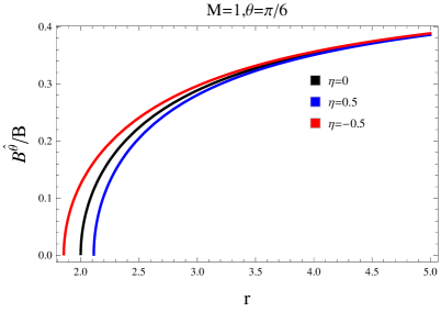
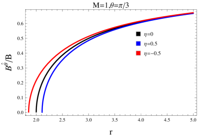
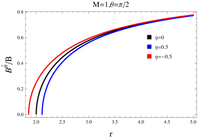
Figure 1: Radial profile of $B^{\hat{\theta}}$ for some values of $\eta$ and $\theta$.

4 The motion of the electric charged particles

This section deals with the circular motion of particles of mass $m$ with charge $e$ around the KZ metric, surrounded by an external uniform magnetic field. Hamilton-Jacobi equation is employed for this purpose and it is given as

$$g^{\mu\nu}\bigg{(}\frac{\partial S}{\partial x^{\mu}}-eA_{\mu}\bigg{)}\bigg{(}\frac{\partial S}{\partial x^{\nu}}-eA_{\nu}\bigg{)}=-m^{2},$$ (11)

where $S$ is the Hamilton-Jacobi action having the following equation

$$S=-Et+L\phi+S_{r}(r)+S_{\theta}(\theta),$$ (12)

with $E$ being energy and $L$ being angular momentum of the particle, receptively. The motion takes place on the equatorial plane ($\theta=\pi/2$). Equation (11) after putting the values, takes the form

$$\left(\frac{-r^{3}}{r^{3}-2Mr^{2}-\eta}\right)E^{2}+\left(\frac{r^{3}-2Mr^{2}-\eta}{r^{3}}\right)g_{rr}^{2}\dot{r}^{2}+\frac{1}{r^{2}}(L-eA_{\phi})^{2}=-m^{2}.$$ (13)

Further simplification, leads to

$$\dot{r}^{2}=\varepsilon^{2}-\left(\frac{r^{3}-2Mr^{2}-\eta}{r^{3}}\right)\left(1+\left(\frac{\mathit{\mathcal{L}}}{r}\mathit{-\omega}_{B}r\right)^{2}\right),$$ (14)

where $\varepsilon=E/m$, $\mathcal{L}=L/m$ be the energy per unit mass, angular momentum per unit mass, respectively, and

$$\mathit{\omega}_{B}=\frac{\mathit{eB}}{2m}.$$ (15)

The $\omega_{B}$ is the cyclotron frequency. It accounts for the magnetic interaction between an electric charge and an external magnetic field. Equation (14) can also be written as

$$\dot{r}^{2}=\varepsilon^{2}-V_{eff},$$ (16)

where

$$V_{eff}=\left(\frac{r^{3}-2Mr^{2}-\eta}{r^{3}}\right)\left(1+\left(\frac{\mathit{\mathcal{L}}}{r}\mathit{-\omega}_{B}r\right)^{2}\right).$$ (17)

The radial plot of $V_{eff}$ has been shown in FIG. (2). The plots show that if we increase values of $\omega_{B}$ and $\eta$, effective potential decreases.

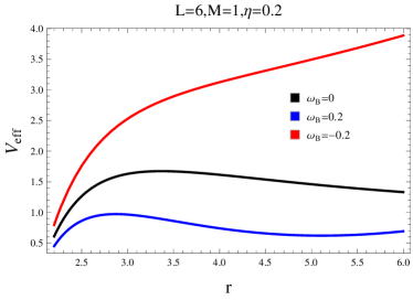
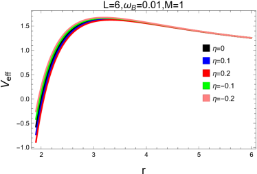
Figure 2: Radial plot of $V_{eff}$. Graph on the left is shown for some values of the cyclotron frequency with other parameters being fixed. The plot in the right panel shown $V_{eff}$ for some values of $\eta$.

For circular motion of the particles, one needs the conditions

$$\dot{r}=0,$$ (18)

$$dV_{eff}/dr=0.$$ (19)

Equation (18) leads to

$$V_{eff}=\varepsilon^{2},$$ (20)

while Eq. (19) gives

$$V_{eff}^{{}^{\prime}} =\frac{1}{r^{6}}\bigg{(}-2Lr^{2}\omega_{B}\left(3\eta+2Mr^{2}\right)+\omega_{B}^{2}\left(-2Mr^{6}+2r^{7}+\eta r^{4}\right)+L^{2}\left(5\eta+6Mr^{2}-2r^{3}\right)$$

$$+2Mr^{4}+3\eta r^{2}\bigg{)}=0.$$ (21)

This gives angular momentum $\mathcal{L}$ as

$$\mathcal{L} =\frac{1}{2(6Mr^{2}-2r^{3}+5\eta)}\bigg{[}4Mr^{4}\omega_{B}+6r^{2}\mathit{\omega}_{B}\eta\pm 2r\big{[}3\eta\left(2r^{3}-5\eta\right)-12M^{2}r^{4}$$

$$+4M(r^{5}-7\eta r^{2})+4r^{2}\omega_{B}^{2}\left(\eta+2Mr^{2}-r^{3}\right)^{2}\big{]}^{1/2}\bigg{]}.$$ (22)

The energy per unit mass $\varepsilon$ is obtained as

$${\LARGE\varepsilon}^{2} = \left(1-\frac{2Mr^{2}+\eta}{r^{3}}\right)$$ (26)

$$\left(1+\left(r\omega_{B}-\frac{4Mr^{4}\omega_{B}+6r^{2}\eta\omega_{B}-\left(\begin{array}[]{c}\left(4Mr^{4}\omega_{B}+6r^{2}\eta\omega_{B}\right)^{2}-4\left(-6Mr^{2}+2r^{3}-5\eta\right)\\ \left(-2Mr^{4}-3r^{2}\eta+2Mr^{6}\omega_{B}^{2}-2r^{7}\omega_{B}^{2}-r^{4}\eta\omega_{B}^{2}\right)\end{array}\right)^{1/2}}{2r\left(6Mr^{2}-2r^{3}+5\eta\right)}\right)^{2}\right).$$

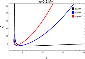
Figure 3: The graph of $\mathcal{L}$ for some values of $\omega_{B}$

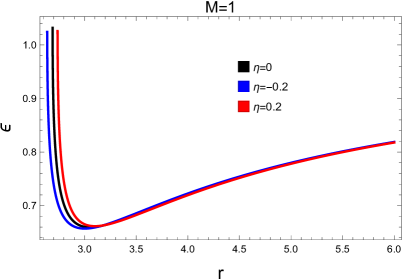
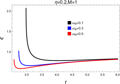
Figure 4: Graph of energy of a charged particle. In the left panel $\omega_{B}=0.3$ with varying values of $\eta$. In the right panel, graph is shown for some values of $\omega_{B}$ with $\eta$ being held fixed.

The graphical behavior of angular momentum is shown in FIG. 3 which shows large values of angular momentum due to $\omega_{B}$. Energy is observed to decrease with $\omega_{B}$ on the right panel of FIG. 4, while, in its left panel, energy is less than the case of Schwarzschild metric.

4.1 The inner most stable circular orbits (ISCO)

To find inner most stable circular orbits or the ISCO, we have $d^{2}V_{eff}/dr^{2}=0.$ This gives

$$\frac{2}{r^{5}\left(6Mr^{2}-2r^{3}+5\eta\right)^{2}}\left(\begin{array}[]{c}\left(\left(6Mr^{2}-2r^{3}+5\eta\right)\left(\begin{array}[]{c}2M\left(6M-r\right)r^{4}+\\ r^{2}\left(20M+3r\right)\eta+15\eta^{2}\end{array}\right)\right)\\ +4r^{2}\left(-2Mr^{2}+r^{3}-\eta\right)\left(\begin{array}[]{c}24M^{2}r^{4}-22Mr^{5}+4r^{6}+\\ 40Mr^{2}\eta-23r^{3}\eta+10\eta^{2}\end{array}\right)\omega_{B}^{2}\\ -2\left(2M\left(6M-r\right)r^{4}+r^{2}\left(20M+3r\right)\eta+15\eta^{2}\right)\omega_{B}\\ \times\sqrt{\begin{array}[]{c}r^{2}\left(2r^{2}\left(-3M+r\right)-5\eta\right)\left(2Mr^{2}+3\eta\right)\\ +4r^{4}\left(2Mr^{2}-r^{3}+\eta\right)^{2}\omega_{B}^{2}\end{array}},\end{array}\right)\geqslant 0.$$

It is impossible to have exact solution for $r_{isco}$, therefore, it is obtained numerically. The numerical solution is shown for various values of $\omega_{B}$ in Table 1. The table shows decreasing $r_{isco}$ with increasing magnetic interaction parameter.

$$\omega_{B}$$

0.4 4.367406

0.45 4.361155

0.5 4.356620

0.55 4.353231

0.6 4.350632

0.65 4.348598

0.7 4.346976

(27)

5 Magnetized Particle Motion

This section deals with the dynamics of magnetized particles around KZ black hole that is immersed in an external asymptotically uniform magnetic field. Modified form of Eq. (11) for motion of magnetized particles is

$$g^{\alpha\beta}\frac{\partial S}{\partial x^{\alpha}}\frac{\partial S}{\partial x^{\beta}}=-\left(m-\frac{1}{2}D^{\alpha\beta}F_{\alpha\beta}\right)^{2},$$ (28)

with $m$ being particle’s mass, $S$ denotes action for magnetized particle in the curved spacetime background. $D^{\mu\nu}$ represents the polarization tensor with the form

$$D^{\alpha\beta}=\eta^{\alpha\beta\mu\nu}u_{\mu}\mu_{\nu},$$ (29)

and has the following constraint

$$\quad D^{\alpha\beta}u_{\beta}=0.$$ (30)

Here $\mu_{\nu}$ denotes the 4-velocity of magnetic dipole moment and $u_{\nu}$ is the 4-velocity of the particles in an arbitrary observer’s rest frame of reference. The product of $D^{\mu\nu}F_{\mu\nu}$ accounts for relationship between the external magnetic field and magnetized particles. In this work, we assume that such an interaction is weak, thus one can neglect $(D^{\mu\nu}F_{\mu\nu})^{2}.$ The Maxwell tensor can be written as

$$F_{\alpha\beta}=2u_{[\mu}E_{\nu]}-\eta_{\alpha\beta\mu\nu}B^{\mu}u^{\nu},$$ (31)

where $E_{\nu}$ and $B_{\nu}$ are the electric and magnetic field, respectively, and $\eta_{\alpha\beta\mu\nu}$ is obtained from the Levi-civita symbol $\epsilon_{\alpha\beta\mu\nu}$ as

$$\eta_{\alpha\beta\mu\nu}=\epsilon_{\alpha\beta\mu\nu}\sqrt{-g},$$ (32)

with $g$ being the determinant of the metric. Taking into account Eqs. (29)-(32) leads to

$$D^{\alpha\beta}F_{\alpha\beta}=2\mu^{\alpha}B_{\alpha}=2\mu^{\hat{\alpha}}B_{\hat{\alpha}}=2\mu B\sqrt{f},$$ (33)

where $f(r)$ is given in Eq. (4). The radial equation of motion is obtained from Eq. (28) and is given as

$$\left(\frac{-r^{3}}{r^{3}-2Mr^{2}-\eta}\right)\varepsilon^{2}+\left(\frac{r^{3}}{r^{3}-2Mr^{2}-\eta}\right)\dot{r}^{2}+\frac{1}{r^{2}}\mathit{\mathcal{L}}^{2}=-\left(1-\frac{\mu B\sqrt{f}}{m}\right)^{2},$$ (34)

$$\dot{r}^{2}=\varepsilon^{2}-\left(\frac{r^{3}-2Mr^{2}-\eta}{r^{3}}\right)\left[(1-\beta\sqrt{f})^{2}+\frac{\mathit{\mathcal{L}}^{2}}{r^{2}}\right],$$ (35)

where $\beta=\frac{\mu B}{m}$ is called magnetic coupling parameter that defines electromagnetic interaction between magnetic dipole and external magnetic field. Equation (35) can be written as

$$\dot{r}^{2}=\varepsilon^{2}-V_{eff},$$ (36)

with $V_{eff}$

$$V_{eff}=\left(\frac{r^{3}-2Mr^{2}-\eta}{r^{3}}\right)\left[(1-\beta\sqrt{f})^{2}+\frac{\mathit{\mathcal{L}}^{2}}{r^{2}}\right].$$ (37)

FIG. 5 shows graph of $V_{eff}$ of Eq. (37). Both the panels show decreasing behavior with increasing $\beta$ (left panel) and $\eta$ (right panel).

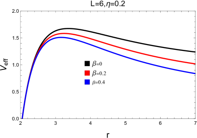
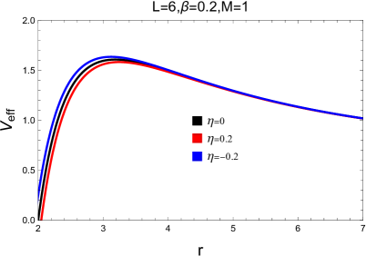
Figure 5: Graphical representation of $V_{eff}$ of radial motion of magnetized particles. On the left, graph is drawn for varying $\beta$. The graph in the right panel has been plotted with varying $\eta$.

To determine the energy and angular momentum, Eqs. (18-20) are again employed. The derivative of $V_{eff}$ is

$$V_{eff}^{{}^{\prime}} =\frac{1}{r^{7}}\Big{[}\mathit{\mathcal{L}}^{2}(6Mr^{3}-2r^{4}+5r\eta)-(2Mr^{2}+3\eta)\big{(}4Mr^{2}\beta^{2}+2\beta^{2}\eta$$

$$+r^{3}\big{(}-1-2\beta^{2}+3\beta\sqrt{f}\big{)}\big{)}\Big{]}$$ (38)

This equation leads to angular momentum $\mathit{\mathcal{L}}^{2}$ as

$$\mathit{\mathcal{L}}^{2}= \frac{1}{6Mr^{3}-2r^{4}+5r\eta}\Big{[}-2Mr^{5}+8M^{2}r^{4}\beta^{2}-4Mr^{5}\beta^{2}-3r^{3}\eta+16Mr^{2}\beta^{2}\eta-6r^{3}\beta^{2}\eta$$

$$+6\beta^{2}\eta^{2}+6Mr^{2}\beta\sqrt{f}+9r^{3}\beta\eta\sqrt{f}\Big{]}.$$ (39)

The expression for energy is

$${\LARGE\varepsilon}^{2}=\frac{(2Mr^{2}-r^{3}+\eta)\left[\begin{array}[]{c}4M^{2}r^{4}\beta^{2}-\beta^{2}\eta^{2}+2r^{6}\left(1+\beta-2\beta\sqrt{f}\right)+r^{3}\eta\left(-2+\beta\left(-\beta+\sqrt{f}\right)\right)\\ +2Mr^{5}\left(-2+3\beta\left(-\beta+\sqrt{f}\right)\right)\end{array}\right]}{6Mr^{8}-2r^{9}+5r^{6}\eta}.$$ (40)

The graphs of angular momentum and energy are shown in FIGs. (6) and (7), respectively. The behavior of angular momentum is increasing with increasing values of $\eta$ and if we increase values of $\beta$, angular momentum and energy decrease.

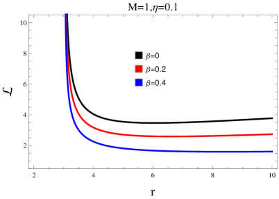
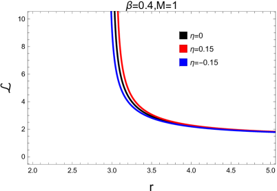
Figure 6: Graph of $\mathit{\mathcal{L}}$ with varying $\beta$ (left panel) and $\eta$ (right panel).

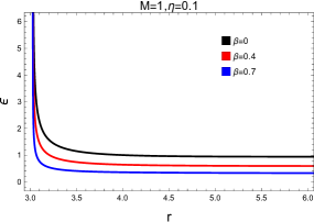
Figure 7: Graphical representation of energy for various values of $\beta$.

The ISCO is given by the equation

$$\frac{1}{r^{7}}\left(\begin{array}[]{c}-\left(2Mr^{2}+3\eta\right)\left(8Mr\beta^{2}+\frac{6Mr^{2}\beta+9\beta\eta}{2r\sqrt{f}}+3r^{2}\left(-1-2\beta^{2}+3\beta\sqrt{f}\right)\right)\\ -4Mr\left(4Mr^{2}\beta^{2}+2\beta^{2}\eta+r^{3}\left(-1-2\beta^{2}+3\beta\sqrt{f}\right)\right)\\ +\frac{\left(2Mr^{2}+3\eta\right)\left(18Mr^{2}-8r^{3}+5\eta\right)\left(4Mr^{2}\beta^{2}+2\beta^{2}\eta+r^{3}\left(-1-2\beta^{2}+3\beta\sqrt{f}\right)\right)}{6Mr^{3}-2r^{4}+5r\eta}\end{array}\right)\geq 0.$$

After simplification, one gets

$$\frac{1}{r^{7}}\left(\begin{array}[]{c}-\left(2Mr^{2}+3\eta\right)\left(8Mr\beta^{2}+\frac{6Mr^{2}\beta+9\beta\eta}{2r\sqrt{f}}+3r^{2}\zeta\right)\\ -4Mr\left(4Mr^{2}\beta^{2}+2\beta^{2}\eta+r^{3}\zeta\right)\\ +\frac{\left(2Mr^{2}+3\eta\right)\left(18Mr^{2}-8r^{3}+5\eta\right)\left(4Mr^{2}\beta^{2}+2\beta^{2}\eta+r^{3}\zeta\right)}{6Mr^{3}-2r^{4}+5r\eta}\end{array}\right)\geq 0.$$

with

$$\zeta=\left(-1-2\beta^{2}+3\beta\sqrt{f}\right).$$ (41)

6 Center of mass energy in the equatorial plane

This section deals with center of mass energy for the collision of particles. The particles are assumed to be having equal masses and are assumed to be coming from infinity with the same initial energy $E_{1}/m_{1}=E_{2}/m_{2}=1$ but with different angular momenta. The center of mass energy for the collision of two particles given by Bañados, Silk and West (BSW) 20a as

$${\Large\varepsilon_{cm}=\frac{{E}_{cm}^{2}}{2m_{0}}=1-g_{\mu\nu}v_{1}^{\mu}v_{2}^{\nu},}$$ (42)

where $v_{i}^{\mu}=(\dot{t}_{i},\dot{r}_{i},\dot{\theta}_{i},\dot{\phi}_{i})$ for $i=1,2$ represent the velocity of the particles.

6.1 The center of mass energy for the collision of two neutral particles

In this subsection, collision of two neutral particles having same rest mass energies will be considered at the equitorial plane. The velocity components in this case are

$$\dot{t}=\frac{r^{3}}{r^{3}-2Mr^{2}-\eta},$$ (43)

$$\dot{\phi}=\frac{l}{r^{2}},$$ (44)

$$\dot{r}^{2}=\varepsilon^{2}-\left(\frac{r^{3}-2Mr^{2}-\eta}{r^{3}}\right)\left(1+\frac{l^{2}}{r^{2}}\right).$$ (45)

The center of mass energy is

$$\varepsilon_{cm} =1+\frac{r^{3}}{r^{3}-2Mr^{2}-\eta}-\frac{l_{1}l_{2}}{r^{2}}$$

$$-\frac{r^{3}}{r^{3}-2Mr^{2}-\eta}\sqrt{1-\left(\frac{r^{3}-2Mr^{2}-\eta}{r^{3}}\right)\left(1+\frac{l_{1}^{2}}{r^{2}}\right)}\sqrt{1-\left(\frac{r^{3}-2Mr^{2}-\eta}{r^{3}}\right)\left(1+\frac{l_{2}^{2}}{r^{2}}\right)},$$ (46)

where $l_{1}$ and $l_{2}$, respectively, represent angular momentum of first and second particle. The radial plot of ${\Large\varepsilon_{cm}}$ is shown in FIG. 8. In FIG. 8 the center of mass energy is decreasing with increasing values of $\eta$ (left) and increasing with increasing values of angular momentum.

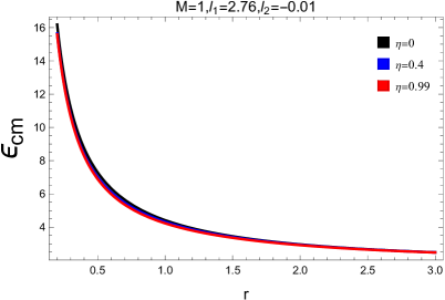
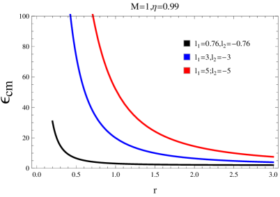
Figure 8: Graph of ${\Large\varepsilon_{cm}}$ for varying $\eta$ (left panel) and angular momentum (right panel).

6.2 The center of mass energy for the collision of two magnetized particles

Here, the collision of two magnetized particles will be considered. The equations for motion in this case are

$$\dot{t}=\frac{r^{3}}{r^{3}-2Mr^{2}-\eta},$$ (47)

$$\dot{\phi}=\frac{l}{r^{2}},$$ (48)

$$\dot{r}^{2}=\varepsilon^{2}-\left(\frac{r^{3}-2Mr^{2}-\eta}{r^{3}}\right)\left((1-\beta\sqrt{f})^{2}+\frac{l^{2}}{r^{2}}\right).$$ (49)

The center of mass energy in this case is

$$\begin{array}[]{c}{\Large\varepsilon}_{cm}^{2}=1+\frac{r^{3}}{r^{3}-2Mr^{2}-\eta}-\frac{l_{1}l_{2}}{r^{2}}-\frac{r^{3}}{r^{3}-2Mr^{2}-\eta}\sqrt{1-\left(\frac{r^{3}-2Mr^{2}-\eta}{r^{3}}\right)\left((1-\beta_{1}\sqrt{f})^{2}+\frac{l_{1}^{2}}{r^{2}}\right)}\times\\ \sqrt{1-\left(\frac{r^{3}-2Mr^{2}-\eta}{r^{3}}\right)\left((1-\beta_{2}\sqrt{f})^{2}+\frac{l_{2}^{2}}{r^{2}}\right)}.\end{array}$$

The graphical behavior is shown in FIG. 9. In FIG. 9 if we decrease values of deformation parameter and angular momentum then the center of mass energy also decreases.

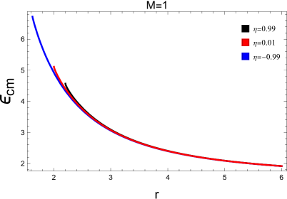
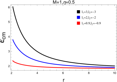
Figure 9: Center of mass energy for the two magnetized particles collision. On left, $l_{1}=2.5,l_{2}=-2.5,\beta_{1}=0.3=\beta_{2}.$ On the right, we have taken $\beta_{1}=0.1=\beta_{2}$.

6.3 The center of mass energy for the collision of a neutral and a magnetized particle

In this subsection, collision of a magnetized and neutral particle has been considered. The equations of motion are given in sections 6.1 and 6.2. The particle 1 is taken to be magnetized and particle 2 is assumed to be neutral. Using these in center of mass energy expression

$${\Large\varepsilon}_{cm}^{2}= 1+\frac{r^{3}}{r^{3}-2Mr^{2}-\eta}-\frac{l_{1}l_{2}}{r^{2}}-\frac{r^{3}}{r^{3}-2Mr^{2}-\eta}$$

$$\times\sqrt{1-\left(\frac{r^{3}-2Mr^{2}-\eta}{r^{3}}\right)\left((1-\beta_{1}\sqrt{f})^{2}+\frac{l_{1}^{2}}{r^{2}}\right)}\sqrt{1-\left(\frac{r^{3}-2Mr^{2}-\eta}{r^{3}}\right)\left(1+\frac{l_{2}^{2}}{r^{2}}\right)}.$$ (50)

The radial profile of ${\Large\varepsilon}$ is shown in FIG. 10. In FIG. 10 if we increase values of $\eta$ center of mass energy increases.

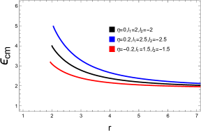
Figure 10: Radial profile of ${\Large\varepsilon}$ with varying $\eta$ and $l_{1}$ and $l_{2}$. Here we have taken $M=1,\beta_{1}=0.2$.

6.4 The center of mass energy for the collision of a charged and a magnetized particle

Here, collision of a magnetized and a charged particle has been considered. The particle 1 is taken to be charged and particle 2 is assumed to be magnetized. Using these in center of mass energy expression, we obtain

$${\Large\varepsilon}_{cm}^{2} =1+\frac{r^{3}}{r^{3}-2Mr^{2}-\eta}-\left(\frac{l_{1}}{r^{2}}-\omega_{B}\right)l_{2}-\frac{r^{3}}{r^{3}-2Mr^{2}-\eta}$$

$$\times\sqrt{1-\left(\frac{r^{3}-2Mr^{2}-\eta}{r^{3}}\right)\left[1+\left(\frac{l_{1}}{r}-\omega_{B}r\right)^{2}\right]\text{ }}\sqrt{1-\left(\frac{r^{3}-2Mr^{2}-\eta}{r^{3}}\right)\left((1{-}\beta\sqrt{f})^{2}{+}\frac{l_{2}^{2}}{r^{2}}\right)}.$$ (51)

The center of mass energy is shown in FIG. 11. In FIG. 11 if we increase values of $\eta$ center of mass energy increases.

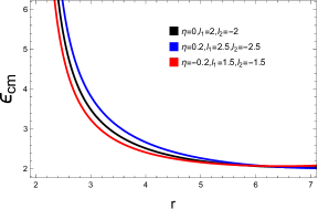
Figure 11: Radial profile of ${\Large\varepsilon}$ with varying $\eta$ and $l_{1}$ and $l_{2}$. Here we have taken $M=1,\omega_{B}=0.1,\beta=0.1$.

7 Summary and conclusion

The Kerr black hole solution is an axisymmetric, stationary and vacuum solution of the Einstein theory of general relativity. All the astrophysical black holes are expected to be described by the Kerr metric. There has been a lot of interest in modified Kerr black hole solutions. Such solutions contain parameters which account for possible deviations from Kerr, which is obtained when deviations are set to zero. One such rotating metric has been developed by Konoplya and Zhidenko kono , whose non-rotating case has been discussed in the present article. In this work, dynamics of charged and magnetized particles (in the equatorial plane) have been discussed in the background of non-rotating Konoplya-Zhidenko metric immersed in an external magnetic field.
First, the effective potential, angular momentum and energy for the circular motion of charged test particles have been studied for the dependence on deformation parameter $\eta$ and cyclotron frequency $\omega_{B}$. In FIG. 2, effective potential has been plotted for varying $\omega_{B}$ (left panel) and $\eta$ (right panel). Both panels show deceasing trend with increasing the respective parameter. This can be explained as the decrease in the least distance between the charged particles and the black hole with increase of $\omega_{B}$ and $\eta$. In FIGs. 3 and 4, radial plots of angular momentum and energy are shown. If we take double derivative of effective potential it give us value of ISCO and it is not possible to find its analytical solution so we just solve it numerically to check its behavior. The table 1. shows the ISCO values at different values of $\omega_{B}$ with $\eta$ fixed. A decreasing trend is observed for this table. Decreasing the ISCO radius is very important because the gravitational potential near the central object can accelerate particles to high energies.

Section 5 contains dynamics of magnetized particle in the background of non-rotating KZ black hole. First the effective has been shown in FIG. 5. The figure shows the same decreasing trend for $\beta$ and $\eta$ as in the charged particles case. Next, angular momentum, energy and ISCO have been studied. In the last section, center of mass energy was studied. The exact expression were shown along with the graphical behavior in each case.

References

- (1) R. M. Wald, Phys. Rev. D 10 1680 (1974).
- (2) A. A. Abdujabbarov, B. J. Ahmedov and V. G. Kagramanova, Gen. Relativ. Gravit. 40 2515 (2008).
- (3) A. N. Aliev and D. V. Gal’tsov, Soviet Phys. Uspekhi 32 75 (1989).
- (4) A. N. Aliev, D. V. Galtsov and V. I. Petukhov, Astrophys. Sp. Sci. 124 137 (1986).
- (5) T. Oteev, A. Abdujabbarov, Z. Stuchlik and B. Ahmedov, Astrophys. Sp. Sci. 361 269 (2016).
- (6) T. Johannsen and D. Psaltis, Phys. Rev. D 83 124015 (2011).
- (7) R. Rahim and K. Saifullah, Ann. Phys. 405 220 (2019).
- (8) U. A. Gillani, R. Rahim and K. Saifullah, Astropart. Phys. 138 102684 (2022).
- (9) R. Rahim and K. Saifullah, IJMPD Doi: 10.1142/S0218271821501236 (2021).
- (10) K. Glampedakis and S. Babak, Class. Quantum Grav. 23 4167 (2006).
- (11) R. Konoplya and A. Zhidenko, Phys. Lett. B 756 350 (2016).
- (12) F. Long. S. Chen, S. Wang and J. Jing, A. Zhidenko, Nucl. Phys. B. 92683 (2018).
- (13) C. Bambi, S. Nampalliwar, Europhys. Lett. 116 30006 (2016); Y. Ni, J. Jiang, C. Bambi, J. Cosmol. Astropart. Phys. 9 14 (2016).
- (14) M. Bañados, J. Silk and S. M. West, Phys. Rev. Lett. 103 (2009) 111102.