Quantum Routing with Teleportation

Abstract

We study the problem of implementing arbitrary permutations of qubits under interaction constraints in quantum systems that allow for arbitrarily fast local operations and classical communication (LOCC). In particular, we show examples of speedups over swap-based and more general unitary routing methods by distributing entanglement and using LOCC to perform quantum teleportation. We further describe an example of an interaction graph for which teleportation gives a logarithmic speedup in the worst-case routing time over swap-based routing. We also study limits on the speedup afforded by quantum teleportation—showing an $O(\sqrt{N\log N})$ upper bound on the separation in routing time for any interaction graph—and give tighter bounds for some common classes of graphs.

I Introduction

Common theoretical models of quantum computation assume that 2-qubit gates can be performed between arbitrary pairs of qubits. However, in practice, scalable quantum architectures have qubit connectivity constraints [1, 2], which forbid long-range gates. These connectivity constraints are typically represented by a graph, where vertices correspond to qubits, and edges indicate pairs of qubits that can undergo 2-qubit gates. Circuits that use all-to-all connectivity must be mapped to new circuits that respect the architecture constraints specified by the graph. Such transformations can introduce polynomial overhead in the circuit depth, so it is crucial to find efficient transformations with low overhead.

A natural approach to mapping circuits to respect interaction constraints is by permuting qubits using routing protocols. Routing refers to the task of permuting packets of information, or tokens, on vertices of a graph. In quantum routing, tokens are data qubits, to be permuted on the graph specified by the architecture’s connectivity constraints. Previous work has used swap gates to perform routing [3, 4], and routing protocols from a classical setting using swap gates [5, 6, 7] can be naturally applied to the problem of routing quantum data as well.

However, while routing can be performed using only swap gates, it may be possible to obtain faster protocols by using a wider range of quantum operations. Previous work has used Hamiltonian evolution [8, 9] to speed up routing. However, these approaches rely on nearest-neighbor quantum interactions, so the routing time is limited by Lieb-Robinson bounds [10, 8]. In this paper, we study quantum routing in systems that allow for ancilla qubits, fast local operations (including measurements), and classical communication (LOCC). Since they can perform fast classical communication across long distances, these systems are not constrained by Lieb-Robinson bounds. Furthermore, even without prior shared entanglement, quantum teleportation can be performed in constant depth by using entanglement swapping [11] in a quantum repeater protocol [12], as shown in Fig. 1. The ability to perform teleportation in constant depth immediately gives routing speedups over swap-based methods and even over previous unitary quantum routing methods, since teleportation can be used to quickly exchange distant pairs of qubits.

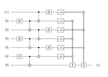
Figure 1: Constant-depth long-range teleportation protocol on a path of 7 qubits. The $X$ and $Z$ gates are classically controlled by the parities of the two sets of measurement results. This protocol can be extended to paths of any length without increasing the circuit depth.

Our work on fast LOCC routing is motivated by previous work that uses LOCC to give low-depth implementations of specific unitaries, such as quantum fanout [13] and preparation of a wide range of entangled states [14, 15, 16, 17]. In fact, previous work has shown routing speedups by using ancillas [18] and by employing LOCC [19]. Using teleportation, Rosenbaum has shown a protocol that implements any permutation in constant depth [19]. However, Rosenbaum’s protocol uses $\Theta(N^{2})$ qubits to perform permutations on $O(N)$ qubits, so that only a negligible fraction of the qubits are data qubits. Engineering qubits is difficult, so it is preferable to use as many of them as possible as data qubits, to enable larger computations. Therefore, in this work we restrict routing protocols to use only $O(1)$ ancillas per data qubit (so in particular, there are $O(N)$ ancillas in total). Rosenbaum’s protocol cannot be performed in this setting. Assuming the availability of $\Theta(1)$ ancillas per data qubit is natural in some quantum systems, such as in NV center qubits [20], quantum dots [21], and trapped ions [22]. Since systems with $\Theta(N^{2})$ ancillas allow for routing in depth $O(1)$, and routing in systems with no ancillas can require depth $\Omega(N)$, systems with $O(N)$ ancillas are also a natural regime in which to investigate the space-time trade-off between the number of ancillas and the routing time. By studying routing in this regime, we make progress on an open question posed by Herbert [18], asking to what extent ancillas can be used to accelerate routing.

In this paper, we examine the advantage of quantum teleportation over classical swap-based routing algorithms. After introducing the models in Sec. II, we discuss known upper and lower bounds on the routing time for both swap-based and teleportation routing in Sec. III. We also introduce an improved algorithm for sparse routing (i.e, routing of a small subset of tokens) with swaps and ancillas. In Sec. IV, we use teleportation to speed up specific permutations. In Sec. V, we compare teleportation routing to swap-based routing for arbitrary permutations, and we give an example of a $(\log N)$-factor speedup over swap-based routing. In Sec. VI, we show an $O(\sqrt{N\log N})$ upper bound on the speedup of teleportation routing over swap-based routing for all graphs, and show tighter bounds for some common classes of graphs. Finally, we conclude in Sec. VII with a discussion of the results and some open questions.

II Preliminaries

We consider architectures consisting of data qubits connected according to a graph $G$ (with vertex set $V(G)$ and edge set $E(G)$), where an edge $(u,v)\in E(G)$ represents a connection between qubits $u,v\in V(G)$. We consider only connected graphs, i.e., graphs in which there is a path from any vertex to any other vertex.

We assume that 2-qubit gates can only be performed between adjacent qubits. We work in discrete time, where a 2-qubit gate between adjacent qubits requires depth 1, and gates between disjoint pairs of qubits can be applied in parallel, i.e., also in depth 1. Further, we allow a constant number of ancillary qubits per data qubit. Gates between data qubits and their associated ancilla qubits are considered to be as fast as single-qubit gates (i.e, can be performed in depth 0). We note, however, that all of our results still apply in the case where gates between data and ancilla qubits take depth 1.

Ancillary qubits corresponding to different data qubits are not directly connected. However, gates between ancillary qubits of neighboring vertices can be performed in depth 1 by swapping ancillas with their corresponding data qubits, performing the desired 2-qubit gate between data qubits, and swapping again with the ancillas. This model can be implemented in realistic quantum architectures with attached ancillas [20, 21, 22] as well as architectures with grid connectivity such as superconducting qubits [23, 1]. For example, Fig. 2a shows an architecture where ancillas are interspersed with data qubits on a grid. This can be represented in our model as Fig. 2b. Both models are equivalent and can simulate each other with only constant depth overhead.

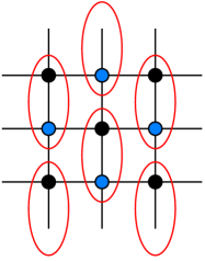
(a)

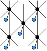
(b)

Figure 2: (a) A grid architecture with ancillas (blue) interspersed between data qubits (black). The red ovals indicate which ancilla corresponds to each data qubit. (b) An equivalent architecture in our model.

The task of routing involves permuting data qubits on the graph. We use the notation

$$\{(1,\pi(1)),(2,\pi(2)),\dots,(N,\pi(N))\}$$ (1)

to denote a permutation on $N$ vertices, where $\pi(i)$ is the vertex to which we must move the $i$th qubit. We also write

$$[N]\coloneqq\{1,2,\dots N\}.$$ (2)

We consider the following models of routing.

1. Swap routing: In this model, the only allowed gates between adjacent qubits are swap gates.

2. LOCC routing: In this model, we are allowed to perform arbitrary 2-qubit gates on disjoint pairs of qubits in a single time step. Further, in the same time step, we are allowed to perform single-qubit measurements (on data and ancilla qubits) and adaptively apply arbitrary single-qubit gates. We refer to this as fast measurement and feedback. Gates in later time steps can be applied adaptively, conditioned on all previous measurement results.

3. Teleportation routing: This model is a specialization of LOCC routing. The ability to perform fast measurement and feedback allows us to perform quantum teleportation, transporting a single qubit to any vertex in constant depth. The entanglement required for quantum teleportation is produced using an entanglement swapping protocol [11], as depicted in Fig. 1. In this model, a swap between the ends of a path can be performed in constant depth by teleporting the qubit at each end to the opposite end, or by performing gate teleportation [24] of a swap gate.

Note that the vertices along a teleportation path cannot be involved in any other operations during a round of teleportation. However, teleportation between multiple pairs of qubits can be performed in parallel if there exist paths for each pair that have no more than a constant number of intersections per vertex, since we allow a constant number of ancilla qubits per data qubit.

We are particularly interested in the routing time $\operatorname{rt}(G,\pi)$, which is the minimum circuit depth to perform the permutation $\pi$ on the data qubits of $G$. The worst-case routing time of a graph $G$ is

$$\operatorname{rt}(G)\coloneqq\max_{\pi\in\mathcal{S}_{|V(G)|}}\operatorname{rt}(G,\pi)$$ (3)

where $\mathcal{S}_{N}$ is the symmetric group, i.e., the group of all permutations of $N$ elements. We let $\operatorname{rt_{tele}}(G)$ denote the routing time in the teleportation model, $\operatorname{rt_{LOCC}}(G)$ denote the routing time in the LOCC model, and $\operatorname{rt_{swap{}}}(G)$ denote the routing time in the swap model.

III Bounds on routing time

In this section, we discuss known bounds on the routing time for both swap and LOCC routing.

III.1 Lower bounds

If a permutation can only be implemented by sending a large number of tokens through a small number of vertices, then any circuit for performing it must have high depth, since each vertex can only hold one token at a time. This gives a natural lower bound on the routing time. To formalize this, we consider the vertex expansion (or vertex isoperimetric number) $c(G)$ of a graph $G$, defined as follows.

Definition 3.1.

The vertex expansion of a graph $G$ is

$$c(G)\coloneqq\min\limits_{X\subseteq V(G)}\frac{|\delta X|}{\min\{|X|,|\overline{X}|\}},$$ (4)

where

$$\overline{X}=V(G)-X$$ (5)

is the complement of $X$, and

$$\delta X=\{v\in\overline{X}\mid\exists\,u\in X\text{ s.t.\ }(u,v)\in E(G)\}$$ (6)

is the vertex boundary of $X$.

Note that $c(G)\leq 1$:

$$\min\limits_{X\subseteq V(G)}\frac{|\delta X|}{\min\{|X|,|\overline{X}|\}}$$ (7)

$$=\min\limits_{X\subseteq V(G)}\left(\frac{|\delta X|}{\min\{|X|,|\overline{X}|\}},\frac{|\delta\overline{X}|}{\min\{|X|,|\overline{X}|\}}\right)$$ (8)

$$=\min\limits_{X\subseteq V(G)}\frac{\min(|\delta X|,|\delta\overline{X}|)}{\min\{|X|,|\overline{X}|\}}$$ (9)

$$\leq 1.$$ (10)

In addition, for a connected graph, since $|\delta X|\geq 1$ and $\min\{|X|,|\overline{X}|\}\leq\frac{N}{2}$ for any $X$, we have $c(G)\geq\frac{2}{N}$ Therefore, for connected graphs, $c(G)\in\left[\frac{2}{N},1\right]$.

Any connected simple graph $G$ satisfies the following.

Theorem 3.2 (Isoperimetric lower bound [8]).

$$\operatorname{rt_{LOCC}}(G) \geq\frac{2}{c(G)}-1.$$ (11)

Since $\operatorname{rt_{swap{}}}(G)\geq\operatorname{rt_{tele}}(G)\geq\operatorname{rt_{LOCC}}(G)$, this lower bound applies to swap- and teleportation-based routing as well.

We can also lower bound the swap-based routing time by the diameter of the graph (i.e, the maximum shortest-path distance between any pair of vertices) since swapping two vertices at distance $d$ requires a swap circuit of depth at least $d$.

Theorem 3.3 (Diameter lower bound).

$$\operatorname{rt_{swap{}}}(G)\geq\operatorname{diam}(G).$$ (12)

Note that this bound does not apply to teleportation or LOCC routing.

III.2 Upper bounds

On any graph, a classical swap algorithm can route on an $N$-vertex tree in depth $O(N)$ [7]. Recall that we only consider connected graphs, so we can always route on a spanning tree with swaps in depth $O(N)$. We thus have the following upper bounds.

Theorem 3.4.

For any $N$-vertex connected graph $G$,

$$\operatorname{rt_{swap{}}}(G)=O(N)$$ (13)

This bound also implies that $\operatorname{rt_{tele}}(G)=O(N)$ and $\operatorname{rt_{LOCC}}(G)=O(N)$.

We can prove a tighter bound for sparse routing. Let $\operatorname{rt_{swap{}}}(G,k)$ denote the worst-case routing time on $G$ over permutations that move at most $k$ tokens. Using reversals, [8] gives a routing algorithm that takes depth $O(\operatorname{diam}(G)+k^{2})$. We improve this result, using swaps with ancillas, to show the following.

Theorem 3.5 (Sparse routing).

For any $N$-vertex connected simple graph $G$ and $k\in[N]$,

$$\operatorname{rt_{swap{}}}(G,k)=O(\operatorname{diam}(G)+k).$$ (14)

Proof sketch.

Call all tokens $v$ with $\pi(v)\neq v$ marked. There are $k$ marked tokens. There are three main steps in our algorithm:

1. Hide all unmarked tokens in the ancillas by performing swaps. Route the $k$ marked tokens to span a tree subgraph in time $O(\operatorname{diam}(G))$.

2. Permute the $k$ tokens on the tree subgraph, using the procedure from [7], in time $O(k)$.

3. Reverse the first step, thereby moving the $k$ tokens from the subgraph to the appropriate target locations in time $O(\operatorname{diam}(G))$. Restore the unmarked tokens from the ancillas.

See Appendix A for the full proof. ∎

IV Faster permutations with teleportation

The ability to perform teleportation immediately suggests possibilities for speedups over swap-based routing. Swap-based routing must obey the diameter lower bound (Theorem 3.3), so permutations that involve long-range swaps (e.g., between diametrically separated pairs of vertices) should be sped up by teleportation.

We define the teleportation advantage for a specific permutation to quantify this speedup:

$$\operatorname{adv}(G,\pi)\coloneqq\frac{\operatorname{rt_{swap{}}}(G,\pi)}{\operatorname{rt_{tele}}(G,\pi)}.$$ (15)

We now consider the following permutation on the path graph $P_{N}$: $\pi_{\mathrm{diam}}=\{(1,N),(2,2),\dots,(N-1,N-1),(N,1)\}$ (see Fig. 3a).

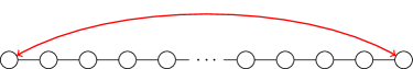
(a) Diameter-length permutation $\pi_{\mathrm{diam}}$ (shown by the red double-sided arrow) on the path graph $P_{N}$ (shown in black).

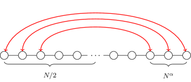
(b) Rainbow permutation $\pi_{\mathrm{rainbow}}^{\alpha}$ (shown by red double-sided arrows) on the path graph $P_{N}$ (shown in black).

Figure 3: Permutations on a 1D lattice

By the diameter lower bound, this permutation takes depth $\Omega(N)$ with swaps. However, with teleportation it takes depth $O(1)$, showing that $\operatorname{adv}(P_{N},\pi_{\mathrm{diam}})=O(N)$.

This further generalizes to permutations that require multiple long-range swaps. For example, consider a rainbow permutation $\pi_{\mathrm{rainbow}}^{\alpha}$, as depicted in Fig. 3b. This permutation involves performing $N^{\alpha}$ swaps across a 1D lattice for some $\alpha\in[0,1]$. With swaps, this takes depth $\Theta(N)$ by the diameter bound, but with teleportation it takes depth $N^{\alpha}$, by a procedure that simply teleports each pair into place sequentially. This gives a polynomial advantage: $\operatorname{adv}(P_{N},\pi_{\mathrm{rainbow}}^{\alpha})=O(N^{1-\alpha})$.

These permutations allow speedups bounded by the diameter of the graph. Any single teleportation step can be simulated by swaps in depth $O(\operatorname{diam}(G))$, by simply swapping along the shortest path between the initial qubit and the final destination. Intuitively, one might therefore expect that teleportation routing could achieve at most a diameter-factor speedup. However, there exist some graphs and permutations for which we can obtain even larger speedups. Teleportation speedups are not limited by the graph diameter since teleportation protocols can utilize multiple longer paths together to avoid intersections.

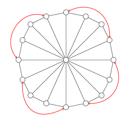
Figure 4: Permutation $\pi_{\mathrm{wheel}}^{l}$ (shown by red double-sided arrows) that exchanges $l$ pairs of vertices on the wheel graph $W_{N+1}$ (shown in black).

To illustrate this, consider the example of a wheel graph $W_{N+1}$, as shown in Fig. 4. The $(N+1)$-vertex wheel graph, with central vertex $N+1$, has edges

$$E(W_{N+1})=\{(u,v)\mid u-v=1\ (\mathrm{mod}\ N)\text{ or }v=N+1\}.$$ (16)

The diameter of $W_{N+1}$ is 2. On this graph, consider the permutation (shown in red in Fig. 4)

$$\pi_{\mathrm{wheel}}^{l}\coloneqq\{ (1,N/l),(N/l+1,2N/l),\ldots,$$ (17)

$$(N-N/l+1,N)\}$$

that exchanges $l$ pairs of vertices spaced along the “rim” of the wheel (assume $l\mid N$). For swap-based algorithms, this can be done in depth $\min\{3l,N/l-1\}$ by routing the qubits sequentially through the central vertex or routing them in parallel along the “rim”, whichever is faster.

This is optimal up to constant factors, by the following reasoning. If there exists a data token that does not pass through the central node, the routing time must be at least $N/l-1$, which is the travel distance along the rim. On the other hand, if every data token passes through the central node, then there must be at least $2l$ steps in the algorithm. Therefore

$$\operatorname{rt_{swap{}}}(W_{N+1},\pi_{\mathrm{wheel}}^{l})\geq\min\{2l,N/l-1\}.$$ (18)

However, in the teleportation routing model, this permutation can be performed in constant depth by performing $l$ teleportations in parallel along non-intersecting paths on the wheel rim. Therefore,

$$\operatorname{rt_{tele}}(W_{N+1},\pi_{\mathrm{wheel}}^{l})=O(1).$$ (19)

Setting $l=\sqrt{N/2}$, we obtain a maximum teleportation advantage $\operatorname{adv}(W_{N+1},\pi_{\mathrm{wheel}}^{l})=\Theta(\sqrt{N})$ for this class of permutations, even though $\operatorname{diam}(W_{N+1})=O(1)$. Teleportation therefore enables super-diametric speedups.

V Teleportation Advantage

While $\pi_{\mathrm{diam}}$, $\pi_{\mathrm{rainbow}}^{\alpha}$, and $\pi_{\mathrm{wheel}}^{l}$ allow for teleportation speedups, they are not the worst-case permutations on their respective graphs. For example, consider the full reflection on the line graph, i.e., a rainbow permutation with $\alpha=1$. This permutation requires depth $\Theta(N)$ for both swap- and teleportation-based routing. Similarly, on the wheel graph with an even number of vertices, the permutation $\pi$ with $\pi(i)=i+\lfloor N/2\rfloor\bmod N$ for all $i\in[N]$ requires depth $\Theta(N)$ for both types of routing as well. Thus, although these graphs have teleportation speedups for specific permutations, there is no separation between their swap and teleportation routing numbers.

To compare the relative strength of the teleportation routing model to the swap-based routing model for all permutations, we aim to understand how much teleportation improves worst-case permutations. We measure the relative strength of the teleportation model by the separation in teleportation and swap-based routing numbers, which we define as the worst-case teleportation advantage:

$$\operatorname{adv}(G)\coloneqq\frac{\operatorname{rt_{swap{}}}(G)}{\operatorname{rt_{tele}}(G)}.$$ (20)

Note that this is not the worst-case ratio of routing numbers for a single specific permutation, i.e., $\operatorname{adv}(G)$ is not necessarily the same as $\max_{\pi}\operatorname{adv}(G,\pi)$. (Indeed, as discussed above, these two quantities differ for the path and wheel graphs.) Instead, $\operatorname{adv}(G)$ can be thought of as the speedup teleportation provides for the general task of routing on a particular graph in the worst case, rather than for implementing a specific permutation. It also allows us to compare different graphs: teleportation routing offers greater worst-case guaranteed speedups on graphs with higher $\operatorname{adv}(G)$.

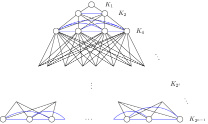
Figure 5: The graph $L(n)$. The black lines show edges between layers, while blue lines show edges within a layer (colored for visibility).

It is not immediately obvious that we should expect $\operatorname{adv}$ to be greater than 1 for any graph. However, we now describe a graph that does offer a worst-case speedup for teleportation. This graph, which we denote by $L(n)$ (with $N=2^{n}-1$ vertices), has $\operatorname{adv}(L(n))=n=\log_{2}(N+1)$. The graph $L(n)$ (depicted in Fig. 5) has

$$V(L(n)) =\{(r,i)\mid r\in[n],i\in[2^{r-1}]\}$$ (21)

and

$$E(L(n))=\begin{aligned} &\begin{aligned} \{&((r,i_{1}),(r,i_{2}))\mid\\ &\quad r\in[n],\,i_{1}<i_{2}\in[2^{r-1}]\}\end{aligned}\\ &\cup\begin{aligned} \{&((r_{1},i_{1}),(r_{2},i_{2}))\mid\\ &\quad r_{2}-r_{1}=1,\,i_{1},i_{2}\in[2^{r-1}]\}.\end{aligned}\end{aligned}$$ (22)

In words, $L(n)$ is a ladder formed by arranging complete graphs $K_{2^{k}}$ for $k\in\{0,1,\ldots,n-1\}$ in horizontal layers, and then connecting every vertex in a given layer with every vertex one layer above or below. The total number of vertices in this graph is

$$N=\sum\limits_{k=0}^{n-1}2^{k}=2^{n}-1.$$ (23)

The diameter of $L(n)$ is exactly $n-1=\log_{2}(N+1)-1$. Theorem 3.3 then implies

$$\operatorname{rt_{swap{}}}(L(n))=\Omega(\log(N)).$$ (24)

With teleportation, we show that routing can be performed in depth $O(1)$. The key idea behind the teleportation protocol is that every layer of $L(n)$ has one more node than all the layers above it together. This allows us to identify a unique node in each layer corresponding to any node from a higher layer. We can then route tokens by simply teleporting along the path formed by the unique nodes from each layer, corresponding to the source vertex of the token to be routed.

This teleportation routing procedure establishes the following.

Proposition 5.1.

$\operatorname{rt_{tele}}(L(n))=O(1)$.

Proof.

For any permutation $\pi\in S_{2^{n}-1}$, we construct a set of paths $\{P(u,\pi(u))\mid u\in V(L(n))\}$ between every node and its destination such that each vertex of the graph belongs to at most four paths in the set.

Label every vertex in the graph with an $n$-bit address as follows. To every node in the subgraph $K_{2^{i}}$ (corresponding to layer $i+1$ of the ladder), assign a unique integer $u$ in the range $[2^{i},2^{i+1}-1]$. (Since the layer is a complete graph, the order within a layer is arbitrary.) Equivalently, we may refer to node $u$ by its binary representation $b(u)$, which is an $(i+1)$-bit string with a leading 1, i.e., of the form $b(u)=(1\ldots)$.

For any vertex $u\in V$, define $r(u,i)$ to be the vertex whose address is $(10^{i-1}b(u))$, i.e., the address of $u$ appended to a leading 1 $i$ places to the left. Note that $r(u,i+1)$ is adjacent to $r(u,i)$ and lies in the layer immediately below $r(u,i)$. Define $r(u,0)=u$.

Now, given two vertices $u,v$ separated by a distance $d$, define a canonical path $P(u,v)=P(v,u)$ as the sequence of the following nodes: $(u,r(u,1),\ldots,r(u,d-1),v)$, where we assume $u<v$ without loss of generality. If $d=1$, then $P(u,v)=(u,v)$. We now show that for any permutation $\pi\in S_{2^{n}-1}$, the set of canonical paths $\{P(u,\pi(u))\mid u\in V(L(n))\}$ intersects any vertex at most four times.

Fix an arbitrary vertex $v$. By construction, $v$ lies in $P(v,\pi(v))$ and $P(v,\pi^{-1}(v))$. Now suppose a path $P(u,\pi(u))$ passes through $v\notin\{u,\pi(u)\}$. Then either $u<v<\pi(u)$ or $\pi(u)<v<u$. Without loss of generality, we assume the former. Since $P(u,\pi(u))$ is canonical, $b(v)=(10^{i}b(u))$ for some $i\geq 0$. Suppose a different path $P(u^{\prime},\pi(u^{\prime}))$ also intersects $v$. Then there are two cases to consider: $u^{\prime}<\pi(u^{\prime})$ and $u^{\prime}>\pi(u^{\prime})$. In the first case, $b(v)=(10^{i^{\prime}}b(u^{\prime}))$. This is only possible when $i=i^{\prime}$ and $u=u^{\prime}$, which implies that $P(u^{\prime},\pi(u^{\prime}))=P(u,\pi(u))$ (giving one intersecting path at $v$). In the second case, the same reasoning implies that $u=\pi(u^{\prime})$. In this case, there are two intersecting paths $P(u,\pi(u))$ and $P(\pi^{-1}(u),u)$ at $v$. Therefore, in addition to $P(v,\pi(v))$ and $P(v,\pi^{-1}(v))$, at most two other paths can intersect at $v$, giving a total of at most four paths.

Finally, construct one Bell pair for every edge in every canonical path $P(u,\pi(u))$, using distinct local ancillas for every pair. The number of Bell pairs shared at any vertex is at most $6=O(1)$, requiring 6 local ancillas per vertex. Using the standard repeater protocol (Fig. 1) along each canonical path, one can then carry out simultaneous teleportation of all data qubits to their destination vertices $v\mapsto\pi(v)$ in constant depth. Therefore, any permutation of the qubits can be implemented in depth $O(1)$. ∎

VI Bounding the Teleportation Advantage

In the previous section, we described a graph with logarithmic teleportation advantage. In this section, we examine limits on the teleportation advantage. In order to understand the power of teleportation in general, we specifically aim to bound the maximum teleportation advantage

$$\operatorname{adv}^{*}\coloneqq\max_{G}\operatorname{adv}(G)$$ (25)

over all graphs with a fixed number of vertices. This quantity measures the maximum speedup teleportation can provide on worst-case permutations for any graph. We also show tighter bounds on the advantage for some common classes of graphs.

We immediately have an upper bound on $\operatorname{adv}$ from LABEL:\swap{}n. Since any teleportation algorithm must have depth $\Omega(1)$, and a swap algorithm can implement any permutation in depth $O(N)$, we have

$$\operatorname{adv}^{*}=O(N).$$ (26)

We now show a tighter bound.

VI.1 Advantage for general graphs

Combining Theorem 3.2 and Theorem 3.3, we have

Lemma 6.1.

$\operatorname{rt_{swap{}}}(G)\geq\max\{\frac{2}{c(G)},\operatorname{diam}(G)\}$.

We now consider the relationship between $\operatorname{diam}(G)$ and $\frac{1}{c(G)}$. Intuitively, increasing the diameter while keeping $|V(G)|$ constant ‘stretches’ the graph, tightening bottlenecks. This causes $c(G)$ to decrease. Similarly, eliminating bottlenecks in the graph requires adding more edges across cuts, thereby increasing the connectivity of the graph and reducing the diameter. We thus expect that graphs with higher diameter will have higher $\frac{1}{c(G)}$, and graphs with small $\frac{1}{c(G)}$ will have small diameter. We can express this relation more precisely as follows.

Lemma 6.2.

For any connected simple graph $G$,

$$\operatorname{diam}(G)\leq 2\frac{\log\frac{N}{2}}{\log\left(1+c(G)\right)}+2.$$ (27)

Proof.

See Appendix B. ∎

One might expect graphs with large diameter to allow large speedups, since the diameter lower bound only applies to swap routing. However, as illustrated by Lemma 6.2, graphs with large diameter also have tight bottlenecks, and therefore, by Theorem 3.2, are not likely to permit large speedups.

We now show our main results bounding the advantage. Our main technical result bounds the advantage in terms of the diameter of the graph. We note that this bound also applies to the separation between swaps and teleportation routing for any permutation, and not just the worst-case separation.

Lemma 6.3.

$\operatorname{adv}(G)=O(\sqrt{N}+\operatorname{diam}(G))$.

Proof.

We construct a swap-based protocol that can simulate a single round of teleportation in depth $O(\sqrt{N}+\operatorname{diam}(G))$, thereby upper bounding the teleportation advantage.

A single round of a teleportation protocol performs teleportation along a set of paths. These paths must intersect no more than a constant number of times per vertex, since there are only a constant number of ancillas per vertex.

For all paths from the teleportation protocol of length at most $\sqrt{N}$, we swap along the paths in parallel. Since each vertex only has a constant number of paths going through it, a qubit can move through every vertex in constant depth. Therefore, these swaps can be performed in depth $O(\sqrt{N})$.

On an $N$-vertex graph, there are $O(N/l)$ paths of length at least $l$. Therefore, since each long path corresponds to a single token, after routing along all paths of length at most $\sqrt{N}$, we have $O(\sqrt{N})$ tokens left to route. By Theorem 3.5, this can be done in depth $O(\sqrt{N}+\operatorname{diam}(G))$.

We can thus simulate each teleportation round in depth $O(\sqrt{N}+\operatorname{diam}(G))$, which completes the proof. ∎

Combining our results, we now have a bound on the advantage for any graph.

Theorem 6.4.

$\operatorname{adv}^{*}=O(\sqrt{N\log N})$.

Proof.

First, combining LABEL:\swap{}n and Theorem 3.2, we have

$$\operatorname{adv}(G)=O(N\cdot c(G)).$$ (28)

Combining this bound with the bound from Lemma 6.3, we have

$$\operatorname{adv}(G)\leq\min\left\{O(N\cdot c(G)),O(\sqrt{N}+\operatorname{diam}(G))\right\}.$$ (29)

We know that $c(G)>0$. Using the fact that $\log(x)\geq 1-1/x$ for $x>0$, we have

$$\frac{1}{\log(1+c(G))}\leq\frac{1}{c(G)}+1=O\left(\frac{1}{c(G)}\right),$$ (30)

where in the last equality we used $c(G)\leq 1$. Applying this to Lemma 6.2 and Eq. 29, we have

$$\operatorname{adv}(G)\leq\min\left\{O(N\cdot c(G)),O\left(\sqrt{N}+\frac{\log(N)}{c(G)}\right)\right\}.$$ (31)

Recall the definition of the maximum teleportation advantage from Eq. 25:

$$\operatorname{adv}^{*}\coloneqq\max_{G}\operatorname{adv}(G).$$ (32)

Therefore,

$$\operatorname{adv}^{*}\leq\max_{G}\min\bigg{\{} O(N\cdot c(G)),$$ (33)

$$O\left(\sqrt{N}+\frac{\log(N)}{c(G)}\right)\bigg{\}}.$$

As $c(G)$ varies, the two bounds in the minimum vary inversely. The first bound, from Eq. 28, is monotonically increasing in $c(G)$ for $c(G)\in(0,1]$. The second bound is monotonically decreasing in $c(G)$ for $c(G)\in\left(0,\frac{\log N}{\sqrt{N}}\right]$. Note that when $c(G)\sim 1/N$ (recall that $c(G)\geq 2/N$), the first bound is smaller, while when $c(G)\sim\frac{\log N}{\sqrt{N}}$, the second bound is smaller. The largest minimum of the two bounds is thus obtained when they are equal.

The minimum of the two bounds is thus maximized when $c(G)=\sqrt{(\log N)/N}$. Note that even if a graph with $c(G)=\sqrt{(\log N)/N}$ does not exist, any other value of $c(G)$ will result in a smaller right-hand side of Eq. 31. With $c(G)=\sqrt{(\log N)/N}$, we obtain

$$\operatorname{adv}^{*}=O\left(\sqrt{N\log N}\right)$$ (34)

as claimed. ∎

This bound applies to any graph, and is thus independent of the diameter of the graph. Therefore, this result shows that in graphs with diameter $\omega(\sqrt{N\log N})$, we cannot obtain a routing time separation between teleportation- and swap-based routing that is proportional to the diameter.

Next we show tighter bounds for a few common families of graphs.

VI.2 Grids

For $d$-dimensional grids (i.e, $P_{n}^{\square d}$, the $d$-fold Cartesian product of the path graph $P_{n}$, with $N=n^{d}$ vertices), the vertex cut bound (Theorem 3.2) gives

$$\operatorname{rt_{LOCC}}(P_{n}^{\square d})\geq\frac{2}{c(P_{n}^{\square d})}-1\geq n-1,$$ (35)

where $c(P_{n}^{\square d})\leq 2/n$ follows from considering a hyperplane that bisects the grid along one dimension. From [5], we have

$$\operatorname{rt_{swap{}}}(G_{1}\square G_{2})=2\operatorname{rt_{swap{}}}(G_{1})+\operatorname{rt_{swap{}}}(G_{2}).$$ (36)

Therefore, the swap routing time of a $d$-dimensional grid is $O(dN^{1/d})=O(dn)$. For constant $d$, this saturates the cut bound in Eq. 35. Therefore, there is no worst-case speedup from either teleportation or full LOCC, i.e, $\operatorname{adv}(P_{n}^{\square d})=1$.

VI.3 Expander graphs

We bound the advantage for spectral expander graphs to be $\operatorname{poly}(\log N)$. The spectral expansion of a graph is given by the first non-zero eigenvalue, $\lambda(G)$, of the graph Laplacian $\mathcal{L}$ with

$$\mathcal{L}_{u,v}=\begin{cases}d_{v}&\text{if }u=v\\ -1&\text{if }(u,v)\in E(G)\\ 0&\text{otherwise},\\ \end{cases}$$ (37)

where $d_{v}$ is the degree of vertex $v$. Spectral expanders are graphs with $\lambda=\Omega(1)$ and bounded degree. For a comprehensive introduction to spectral graph theory, consult [6].

To bound the advantage for spectral expanders, we first use the following upper bound on the swap-based routing number. Let $d_{*}\coloneqq\frac{\max_{v\in V}d_{v}}{\min_{v\in V}d_{v}}$ denote the degree ratio of a graph.

Theorem 6.5 ([8]).

For any graph $G$ and permutation $\pi$,

$$\operatorname{rt_{swap{}}}(G,\pi)=O\left(\frac{d_{*}}{\lambda(G)^{2}}\log^{2}N\right).$$ (38)

Combining this result with the lower bound of Theorem 3.2, we immediately get

$$\operatorname{adv}(G)=O\left(\frac{d_{*}c(G)\log^{2}N}{\lambda(G)^{2}}\right).$$ (39)

Thus graphs with $\lambda(G)=\Omega(1)$ and $d_{*}=O(1)$ (such as spectral expanders) have at most a polylogarithmic advantage.

VI.4 Hypercubes

The swap-based routing time for a $d$-dimensional hypercube $Q_{d}$ is [5, 25]

$$\operatorname{rt_{swap{}}}(Q_{d})=\Theta(d).$$ (40)

Since $|V(Q_{d})|=N=2^{d}$,

$$\operatorname{rt_{swap{}}}(Q_{d})=\log N.$$ (41)

Now, we will show that $c(Q_{d})=\Theta(\frac{1}{\sqrt{d}})$. In a hypercube, Hamming balls (i.e., sets of all points with Hamming weight $\leq r$ for some integer $r$) have the smallest boundary of all sets of a given size [26]. Taking the Hamming ball of radius $d/2$ as $X$, we have $|X|=2^{d-1}$ and $|\delta X|=\binom{d}{d/2}=\Theta(2^{d}/\sqrt{d})$. Therefore, $c(G)=\Theta(1/\sqrt{d})$. Using Theorem 3.2, we have $\operatorname{rt_{tele}}(G)=\Omega(\sqrt{d})=\Omega(\sqrt{\log N})$. Teleportation thus offers at most an $O(\sqrt{\log N})$ advantage on hypercubes.

VI.5 Other graphs

The cyclic butterfly graph $B_{r}$ has been proposed as a constant-degree interaction graph that allows for fast circuit synthesis [3, 27]. Each of the $N=r2^{r}$ vertices is labelled $(w,i)\in\{0,1\}^{r}\times[r]$. Vertices $(w,i)$ and $(v,i+1\bmod r)$ are connected if $w=v$ or if $w$ and $v$ differ by exactly one bit in the $i$th position. The cyclic butterfly has diameter $O(\log N)$, degree 4, and $\operatorname{rt_{swap{}}}(B_{r})=O(\log N)$ [27].

We now show that the $O(\log N)$ protocol is optimal even for teleportation routing on the cyclic butterfly graph, so $\operatorname{adv}(G)=O(1)$. Bipartition the vertices into sets $X,\overline{X}$ such that $X$ consists of all rows with bit $j=0$ for some $j$, and $\overline{X}$ consists of all rows with bit $j=1$. For this partition, $|X|=r2^{r-1}$ and $|\delta X|=2^{r}$, so $c(G)\leq 2/r$. Since $r=\Theta(\log N)$, $c(G)=O(\frac{1}{\log N})$, so from Theorem 3.2, $\operatorname{adv}(G)=O(1)$.

The complete graph $K_{N}$ has $\operatorname{rt_{swap{}}}(K_{N})=O(1)$, and therefore has $\operatorname{adv}(K_{N})=1$.

Finally, graphs with poor expansion properties—in particular, with vertex expansion $c(G)=O(\frac{\operatorname{poly}(\log N)}{N})$—have at most polylogarithmic advantage by Eq. 28.

VII Discussion

In this paper, we have used quantum teleportation to speed up the task of permuting qubits on graphs. We have shown examples of specific types of permutations that can be sped up by teleportation. Further, we have shown an example of a graph that exhibits a worst-case teleportation routing speedup of $\log N$. Our main technical result (Theorem 6.4) is a general upper bound of $O(\sqrt{N\log N})$ on the worst-case routing speedup.

These results lead to two natural open questions:

1. Does there exist a graph with $\operatorname{adv}(G)=\omega(\log N$)?

2. Is there a tighter upper bound than Theorem 6.4 on the maximum teleportation advantage for any graph?

We expect that both of these questions can be answered positively. Our upper bound on teleportation advantage was derived by showing a procedure to simulate a single round of a teleportation protocol with swaps. We believe that there should be more sophisticated methods to perform the conversion that give tighter bounds by exploiting parallelism. A possible approach to tightening this bound would be to show a swap protocol that parallelizes performing routing from multiple teleportation rounds, since swap paths need not obey the strict conditions of teleportation paths (namely, allowing only a constant number of path intersections per vertex).

A graph with a superlogarithmic separation between swap- and teleportation-based routing (if one exists) cannot be a spectral expander, as per Theorem 6.5. From Lemma 6.2, we know that a graph with large diameter will have poor expansion properties (small $c(G)$) and therefore will not have a large teleportation advantage as per Eq. 28. Some candidate graphs for a superlogarithmic teleportation advantage are those with $c(G)\approx\sqrt{(\log N)/N}$. Such graphs may come closer to achieving a teleportation advantage given by the upper bound of Theorem 6.4.

We have primarily focused on the teleportation model of routing. However, teleportation routing is a special case of the more general LOCC model of routing. We currently do not know whether the full power of LOCC can provide a super-constant speedup over teleportation routing. This is analogous to another open question, namely whether routing with arbitrary 2-qubit gates—or even with arbitrary bounded 2-qubit Hamiltonians—can provide a super-constant speedup over swap-based routing [8].

Herbert [18] posed the question of establishing to what extent ancillas can be used to reduce the routing depth. Rosenbaum [19] showed an $O(1)$ routing protocol on $N$ qubits with $\Theta(N^{2})$ ancillas (i.e., an advantage of $O(N)$), while systems without ancillas cannot perform LOCC or teleportation routing, and therefore cannot exhibit any speedups. We have investigated an intermediate regime, and have shown that a linear number of ancillas cannot allow for speedups greater than $O(\sqrt{N\log N})$. It remains an open question to further investigate the space-time tradeoff between the number of ancilla qubits and the routing time.

A more general task than routing is to perform unitary synthesis, i.e, decompose a particular unitary into 2-qubit gates that can be applied on our locality-constrained qubits. It remains an open question to understand how much unitary synthesis can be sped up by using LOCC with a linear number of ancillary qubits. Previous work has shown an $\Omega(N)$ speedup for implementing fanout [13] and preparing GHZ and W states [14], and an $\Omega(\sqrt{N})$ speedup for preparing toric code states [14], which takes time $\Omega(\sqrt{N})$ without LOCC [28]. Previous work has also shown how measurements of cluster states can be used to efficiently prepare long-range entanglement [16] and states with exotic topological order [17]. In principle, LOCC could similarly provide polynomial speedups for unitary synthesis, as we currently have no upper bounds on the advantage for any unitary.

Appendix A Sparse routing

Previous work [8] shows an $O(\operatorname{diam}(G)+k^{2})$ swap-based routing algorithm to route $k$ vertices on a graph $G$. In this Appendix, we show that using swaps with a constant number of ancillas per qubit, this result can be improved to be linear in $k$.

(a) Line 2

(b) Line 4

(c) Line 5

(d) Line 7

(e) Line 8

(f) Advanced train

Figure 6: Advancing a train of tokens, as in Algorithm A.1. Blank vertices hold state $\ket{0}$. The dashed lines represent connections with the local ancilla qubits.

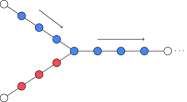
(a) The blue train advances one vertex at a time.

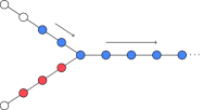
(b) The red train waits for the blue train, but remains in the same connected token cluster.

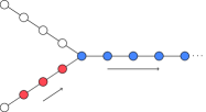
(c) The red train is concatenated to the blue train.

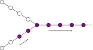
(d) Once concatenated, they move as a single train.

Figure 7: Joining trains of tokens.

We first introduce the following definitions.

Definition 1.1 (Null token).

A null token is a dummy token that can be routed anywhere. In quantum routing, all ancillas are initialized with a null token in state $\ket{0}$.

Definition 1.2 (Train).

A train is a set of non-null tokens along a path subgraph of $G$.

Input : Train $T$ from vertices $0$ to $l-1$ on a path. Vertex $l$ has a null token. The data token on vertex $i$ is data$(i)$, and the token on the corresponding ancilla is ancilla$(i)$.

1 parallel for $i=1,3,\dots$ :

2      swap data$(i)$ with ancilla$(i)$;

3      

4parallel for $i=0,2,4,\dots$ :

5      swap data($i$) with data($i+1$);

6       swap data($i+1$) with ancilla$(i+1)$;

7      

8parallel for $i=1,3,\dots$ :

9      swap data($i$) with data($i+1$);

10       swap data($i$) with ancilla($i$);

11      

Algorithm A.1 Advance a train

Now we show how a train can advance, i.e., translate by 1 along its length.

Lemma 1.3.

A train can advance in depth 5.

Proof.

Suppose we want to move a train of length $l$ towards some vertex $r$. We define the head of a train as the token on the vertex closest to $r$, and the tail as the token on the vertex furthest from $r$. Consider the path subgraph spanned by the vertices the train lies on as well as the vertices of the shortest path from the head to $r$. Let the tail lie on vertex $0$, and head lie at vertex $l-1$. We use Algorithm A.1 to advance the train such that after 5 time steps, the tail of the train is at vertex $1$ and the head at $l$. This procedure is depicted in Fig. 6. ∎

Input : Set of token clusters; vertex $r$.

1 In each token cluster, advance the train with head closest to $r$ by 1 using Algorithm A.1.;

2 If any two token clusters are adjacent, join them as a single token cluster.;

3 If the head of any train $T_{1}$ is adjacent to the tail of another train $T_{2}$, join them as a single train with the head of $T_{2}$ and the tail of $T_{1}$.;

Algorithm A.2 Token cluster movement

We now define a token cluster.

Definition 1.4 (Token cluster).

A token cluster is a set of trains such that each train contains a token on a vertex that is adjacent to a vertex with a token from another train in the token cluster.

Token clusters move as in Fig. 7, by Algorithm A.2. Once a train joins a token cluster, it remains connected and part of the token cluster.

We now prove Theorem 3.5, which we reproduce here for clarity.

See 3.5

Proof.

Let us call the $k$ tokens on vertices

$$\{v\in V(G)\mid\pi(v)\neq v\}$$ (42)

marked tokens, and let the remaining token be unmarked tokens. Our algorithm involves three phases.

Phase 1: First, we swap the unmarked tokens into local ancilla qubits and store them there for the duration of routing. Every vertex that initially held an unmarked token now holds a null token.

Next, we select some vertex $r$ of $G$ arbitrarily (in practice, selecting $r$ to be at the center of the graph may provide constant-factor speedups). We now move all marked tokens towards vertex $r$ by swapping along the shortest possible paths, until the tokens span a set of vertices forming a tree connected to $r$. The tokens are moved in parallel, and when their paths intersect, the tokens move as trains, as per Lemma 1.3. When the paths of multiple trains intersect, they form a token cluster, and can be moved as in Algorithm A.2.

Any given train is at most $\operatorname{diam}(G)$ distance away from $r$ at the start of Phase 1. At every time step, a train either advances by 1 vertex towards $r$, or is part of a token cluster in which another train closer to $r$ advances. Therefore, every token cluster becomes connected to $r$ in depth $O(\operatorname{diam}(G))$, since in every token cluster, at least 1 train must reach $r$ in depth $O(\operatorname{diam}(G))$. In particular, in $O(\operatorname{diam}(G))$ depth, all non-null tokens must span a tree containing $r$, and thus have merged into a single token cluster.

Phase 2: Now we have $k$ vertices spanning a tree $T$. Suppose token $v$ is mapped to the vertex $t(v)$ in $T$ after Phase 1. Note that the token $u$ that was originally at $t(v)$ must also be a marked token, and therefore must now lie in $T$. We route the tokens on $T$ according to a permutation $\pi^{\prime}$ such that

$$\pi^{\prime}(t(v))\coloneqq t(\pi(v))$$ (43)

for all $t(v)\in V(T)$, in depth $2k$ [5].

Phase 3: We now simply perform Phase 1 in reverse. During Phase 1, the marked token at $u$ was mapped to $t(u)$. Therefore, after Phase 3, the token at $t(u)$ is mapped to vertex $u$. Therefore, the following mapping is applied to all vertices with marked tokens:

$$u\xrightarrow{\text{Phase 1}}t(u)\xrightarrow{\text{Phase 2}}t(\pi(u))\xrightarrow{\text{Phase 3}}\pi(u).$$ (44)

The combined depth of the three phases is at most $O(k+\operatorname{diam}(G))$. ∎

Appendix B Proof of diameter-expansion trade-off

In this appendix, we prove Lemma 6.2, adapting Proposition 3.1.5 from [29] to vertex neighborhoods rather than edge neighborhoods.

See 6.2

Proof.

For any vertex $v\in V$, denote by $C(v,k)$ the set of all vertices that are at distance $k$ from $v$. We call $C(v,k)$ a circle of radius $k$ centered on $v$. Note that $C(v,k)\cap C(v,k^{\prime})=\emptyset$ when $k\neq k^{\prime}$. Next, define

$$D(v,k)\coloneqq\bigcup\limits_{r=0}^{k}C(v,r)$$ (45)

to be the disk of radius $k$ centered on $v$. Observe that $C(v,0)=D(v,0)=\{v\}$. Finally, choose an integer $\rho(v)$ such that $|D(v,\rho(v))|\leq N/2<|D(v,\rho(v)+1)|$ and call it the horizon of $v$. For any vertex, a horizon exists and is an integer between 0 and $\operatorname{diam}(G)-1$.

By definition, for all $k\leq\rho(v)+1$, we have

$$|C(v,k)|\geq c(G)\cdot|D(v,k-1)|.$$ (46)

Applying this inequality gives

$$|D(v,\rho(v))| =|C(v,\rho(v))|+|D(v,\rho(v)-1)|$$ (47)

$$\geq(1+c(G))|D(v,\rho(v)-1)|.$$ (48)

Recursing until we reach the base case $D(v,0)=\{v\}$, we obtain

$$N/2\geq(1+c(G))^{\rho(v)},$$ (49)

giving

$$\rho(v)\leq\frac{\log(N/2)}{\log(1+c(G))}.$$ (50)

Next, for any two vertices $u,v\in V$, let $d(u,v)$ denote the distance between $u,v$. We claim that

$$d(u,v)\leq\rho(u)+\rho(v)+2.$$ (51)

To see this, note that by definition, $|D(u,\rho(u)+1)|>N/2$ and $|D(v,\rho(v)+1)|>N/2$, which implies that $D(u,\rho(u)+1)\bigcap D(v,\rho(v)+1)\neq\emptyset$ by the pigeonhole principle. Therefore, there exists a vertex $t$ such that $d(u,t)\leq\rho(u)+1$ and $d(t,v)\leq\rho(v)+1$. By the triangle inequality, we have $d(u,v)\leq\rho(u)+\rho(v)+2$ as claimed.

Finally, we use Eq. 50 and maximize the distance over all vertex pairs $u,v$ to get

$$\operatorname{diam}(G)\leq\frac{2\log(N/2)}{\log(1+c(G))}+2$$ (52)

as claimed. ∎

References

- Arute et al. [2019] F. Arute, K. Arya, R. Babbush, D. Bacon, J. C. Bardin, R. Barends, R. Biswas, S. Boixo, F. G. S. L. Brandao, D. A. Buell, and et al., Quantum supremacy using a programmable superconducting processor, Nature 574, 505–510 (2019).
- Monroe and Kim [2013] C. Monroe and J. Kim, Scaling the ion trap quantum processor, Science 339, 1164–1169 (2013).
- Cowtan et al. [2019] A. Cowtan, S. Dilkes, R. Duncan, A. Krajenbrink, W. Simmons, and S. Sivarajah, On the qubit routing problem, in TQC 2019, LIPIcs, Vol. 135 (2019) pp. 5:1–5:32.
- Childs et al. [2019] A. M. Childs, E. Schoute, and C. M. Unsal, Circuit transformations for quantum architectures, in TQC 2019, LIPIcs, Vol. 135 (2019) pp. 3:1–3:24.
- Alon et al. [1994] N. Alon, F. R. K. Chung, and R. L. Graham, Routing permutations on graphs via matchings, SIAM J. Discrete Math. 7, 513 (1994).
- Chung [1996] F. Chung, Spectral Graph Theory (American Mathematical Society, 1996).
- Zhang [1999] L. Zhang, Optimal bounds for matching routing on trees, SIAM J. Discrete Math. 12, 64 (1999).
- [8] A. Bapat, A. M. Childs, A. V. Gorshkov, and E. Schoute, Advantages and limitations of quantum routing, in preparation.
- Bapat et al. [2021] A. Bapat, A. M. Childs, A. V. Gorshkov, S. King, E. Schoute, and H. Shastri, Quantum routing with fast reversals, Quantum 5, 533 (2021).
- Lieb and Robinson [1972] E. H. Lieb and D. W. Robinson, The finite group velocity of quantum spin systems, Commun. Math. Phys 28, 251–257 (1972).
- Żukowski et al. [1993] M. Żukowski, A. Zeilinger, M. A. Horne, and A. K. Ekert, “event-ready-detectors” bell experiment via entanglement swapping, Phys. Rev. Lett. 71, 4287 (1993).
- Briegel et al. [1998] H.-J. Briegel, W. Dür, J. I. Cirac, and P. Zoller, Quantum repeaters: The role of imperfect local operations in quantum communication, Phys. Rev. Lett. 81, 5932 (1998).
- Pham and Svore [2013] P. Pham and K. M. Svore, A 2d nearest-neighbor quantum architecture for factoring in polylogarithmic depth, QIC 13, 937 (2013).
- Piroli et al. [2021] L. Piroli, G. Styliaris, and J. I. Cirac, Quantum circuits assisted by local operations and classical communication: Transformations and phases of matter, Phys. Rev. Lett. 127, 220503 (2021).
- Eldredge et al. [2020] Z. Eldredge, L. Zhou, A. Bapat, J. R. Garrison, A. Deshpande, F. T. Chong, and A. V. Gorshkov, Entanglement bounds on the performance of quantum computing architectures, Phys. Rev. Research 2, 033316 (2020).
- Tantivasadakarn et al. [2022] N. Tantivasadakarn, R. Thorngren, A. Vishwanath, and R. Verresen, Long-range entanglement from measuring symmetry-protected topological phases (2022), arXiv:2112.01519 [cond-mat.str-el] .
- Verresen et al. [2022] R. Verresen, N. Tantivasadakarn, and A. Vishwanath, Efficiently preparing schrödinger’s cat, fractons and non-abelian topological order in quantum devices (2022), arXiv:2112.03061 [quant-ph] .
- Herbert [2020] S. Herbert, On the depth overhead incurred when running quantum algorithms on near-term quantum computers with limited qubit connectivity, QIC 20, 787 (2020), 1805.12570v5 .
- Rosenbaum [2013] D. J. Rosenbaum, Optimal quantum circuits for nearest-neighbor architectures, in TQC 2013, LIPIcs, Vol. 22 (2013) pp. 294–307.
- Dutt et al. [2007] M. V. G. Dutt, L. Childress, L. Jiang, E. Togan, J. Maze, F. Jelezko, A. S. Zibrov, P. R. Hemmer, and M. D. Lukin, Quantum register based on individual electronic and nuclear spin qubits in diamond, Science 316, 1312–1316 (2007).
- Loss and DiVincenzo [1998] D. Loss and D. P. DiVincenzo, Quantum computation with quantum dots, Phys. Rev. A 57, 120 (1998).
- Bruzewicz et al. [2019] C. D. Bruzewicz, R. McConnell, J. Stuart, J. M. Sage, and J. Chiaverini, Dual-species, multi-qubit logic primitives for Ca+/Sr+ trapped-ion crystals, NPJ Quantum Inf. 5, 1–10 (2019).
- Nation et al. [2021] P. Nation, H. Paik, A. Cross, and Z. Nazario, The IBM Quantum heavy hex lattice (2021).
- Gottesman and Chuang [1999] D. Gottesman and I. L. Chuang, Demonstrating the viability of universal quantum computation using teleportation and single-qubit operations, Nature 402, 390–393 (1999).
- Li et al. [2010] W.-T. Li, L. Lu, and Y. Yang, Routing numbers of cycles, complete bipartite graphs, and hypercubes, SIAM J. Discrete Math. 24, 1482–1494 (2010).
- Harper [1966] L. Harper, Optimal numberings and isoperimetric problems on graphs, Journal of Combinatorial Theory 1, 385 (1966).
- Brierley [2017] S. Brierley, Efficient implementation of quantum circuits with limited qubit interactions, QIC 17, 1096 (2017), 1507.04263 .
- Bravyi et al. [2006] S. Bravyi, M. B. Hastings, and F. Verstraete, Lieb-Robinson bounds and the generation of correlations and topological quantum order, Phys. Rev. Lett. 97, 050401 (2006).
- Kowalski [2019] E. Kowalski, An introduction to expander graphs (Société Mathématique de France, 2019).