Reproducibility and Baseline Reporting for Dynamic Multi-objective Benchmark Problems

Abstract.

Dynamic multi-objective optimization problems (DMOPs) are widely accepted to be more challenging than stationary problems due to the time-dependent nature of the objective functions and/or constraints. Evaluation of purpose-built algorithms for DMOPs is often performed on narrow selections of dynamic instances with differing change magnitude and frequency or a limited selection of problems. In this paper, we focus on the reproducibility of simulation experiments for parameters of DMOPs. Our framework is based on an extension of PlatEMO, allowing for the reproduction of results and performance measurements across a range of dynamic settings and problems. A baseline schema for dynamic algorithm evaluation is introduced, which provides a mechanism to interrogate performance and optimization behaviours of well-known evolutionary algorithms that were not designed specifically for DMOPs. Importantly, by determining the maximum capability of non-dynamic multi-objective evolutionary algorithms, we can establish the minimum capability required of purpose-built dynamic algorithms to be useful. The simplest modifications to manage dynamic changes introduce diversity. Allowing non-dynamic algorithms to incorporate mutated/random solutions after change events determines the improvement possible with minor algorithm modifications. Future expansion to include current dynamic algorithms will enable reproduction of their results and verification of their abilities and performance across DMOP benchmark space.

1. Introduction

Optimisation of competing goals is the basis of multi-objective optimization. This is made more difficult when a time-dependent component is introduced, creating a dynamic multi-objective optimization problem (DMOP). There has been considerable work in the past two decades focused on the design of benchmark problems, the development of algorithms, performance measurements and visualization, however, there is limited understanding of the parameters controlling the dynamics. Existing works promote the use of a diverse problem set but carry out experiments for a limited range of the parameters controlling dynamic changes - restricting the true scope of any conclusions made.

Some of the principal benchmark dynamic multi-objective optimization problems (DMOPs) were defined nearly two decades ago by Farina et al. (Farina et al., 2003). Since then, a plethora of benchmark problems have been proposed (Jiang and Yang, 2017; Helbig and Engelbrecht, 2013a; Ruan et al., 2021; Jiang et al., 2019; Zhang et al., 2021b, a; Tang et al., 2007; Huang et al., 2011; Yazdani et al., 2020; Chen et al., 2018; Gee et al., 2017), allowing for the testing of different characteristics of real world systems in a controllable environment. Dynamic Optimization Problem (DOP) generators such as Moving Peaks (Branke, 1999; Yazdani et al., 2020) and the Dynamic XOR (Yang, 2003) and others are well-known single-objective environments in which the difficulty of a problem instance can be controlled by increasing the number of peaks or bits respectively. Comprehensive surveys of methods, measurements and problems are given in (Nguyen et al., 2012; Branke, 2002; Branke and Schmeck, 2003; Azzouz et al., 2016; Raquel and Yao, 2013; Helbig and Engelbrecht, 2013a, b).

In existing dynamic multi-objective benchmarks, defining the ‘difficulty’ of a particular problem or instance can be linked to characteristics of the dynamics in the problem. Farina et al. (Farina et al., 2003) defined a four-type system according to whether the dynamics alter the: (I) Pareto-Optimal Set (POS), (III) Pareto-Optimal Front (POF), both (II) or neither (IV). Meanwhile, Nguyen et al. (Nguyen et al., 2012) suggests a broader framework for DOPs to classify problems based on whether they have the following properties: Time-linkage; predictability of changes; visibility of dynamics to the optimization algorithm; constraints or dynamic constraints; single or multiple objectives; periodical, recurrent or cyclic dynamics and type and factor of dynamic changes (e.g. objective functions, decision variable domain or number). Azzouz et al. (Azzouz et al., 2017) suggests a streamlined version of this for DMOPs that, in addition to the POS/POF observations, problems can be grouped based on the frequency, severity or predictability of changes.

Nevertheless, despite these frameworks for classifying the proposed benchmarks, there is little associated literature outlining the consistency of parameter settings and reproducibility of results on DMOPs. For researchers attempting to find a DMOP benchmark suite with characteristics similar to a real world problem under investigation, the baseline ‘difficulty’ of the parameters pertaining to the dynamics and the problem are under-documented. Whilst the recently proposed comprehensive benchmark sets SDP (Jiang et al., 2019), RDP (Ruan et al., 2021) and JY (Jiang and Yang, 2017), offer a multitude of well-designed and diverse benchmarks, the results presented examine a limited ranges of dynamic parameters in terms of severity and frequency of changes.

Many works use non-dynamic MOEAs (designed originally for static problems) to compare and contrast the performance of their proposed DMOEA (Chen et al., 2018; Gee et al., 2017; Mehnen et al., 2006; Zhang et al., 2021b; Jiang et al., 2019). Some of these feature simple modifications to handle dynamic changes such as restarting or introducing random solutions. However the detriment or benefit of such modifications relative to the standard implementation of these MOEAs is unknown. Understanding the capability of MOEAs for DMOPs in a fine-grained experimentation of frequency and severity will allow us to determine the validity of prior application.

In order to determine a baseline difficulty for existing dynamic multi-objective benchmarks there are some key parameters, on which we can determine the baseline performance of state of the art static MOEAs. We argue, that it is essential a systematic examination of the dynamic problem parameters – severity and frequency – is carried out. Such an examination would provide insights into how specific algorithms and simple response mechanisms can cope with the changing dynamics, thus allowing for a definition of a baseline range of parameters for a given DMOPs that cannot effectively be handled by existing MOEAs. Here, using a subset of established DMOPs, we illustrate the importance of the frequency and severity parameters through a fine-grained experimental protocol across ranges of these parameters that encompass the commonly used values in the literature. There exists a framework called PlatEMO (Tian et al., 2017) which gathers a comprehensive library of multi-objective optimization problems and Evolutionary Algorithms (EAs) designed to solve them. This provides the inspiration for the collation of DMOPs, and in further work, the collation of the vast range of DMOEAs currently in the literature. By providing the tools we employ to generate our results, we facilitate future consistency and therefore verification, corroboration and comparison of results. The proposed schema for determining the maximum capability of MOEAs on DMOPs provides the framework for determining the dynamic instances of problems that novel DMOEAs should be tested on to determine meaningful improvements over existing methods.

To summarise the contributions of this paper:

• Firstly, we provide an experimental schema allowing for the reproducibility of results for DMOPs, including the DPTP, a platform allowing for fine-grained experimentation of DMOP parameters.

• Additionally, we perform for a selection of typical benchmark DMOPs, an investigation of parameters values commonly used in the literature that govern the frequency and severity of changes.

• We examine the performance of non-dynamic MOEAs on these parameters to ascertain a minimum recommended experimental range for frequency and severity, below which good performance can be achieved by non-dynamic MOEAs.

• The utility of commonly used simple modifications to static MOEAs (random and mutated solution additions) is contrasted to the random restart methodology which is widely used as baseline comparison for novel algorithm performance.

The remainder of the paper is organized as follows. Section 2 contains a summary of DMOP definitions including the frequency and severity parameters, together with their usage and the usage of MOEAs on DMOPs in the literature. Section 3 gives an overview of the experimental platform and the problems, algorithms, responses and parameter ranges used. Section 4 details the key results pertaining to each of the contributions listed above. Conclusions are drawn in Section 5.

2. Background

2.1. Dynamic multi-objective Optimization Problems

Dynamic multi-objective optimization problems extend multi-objective problems to include time-variant terms or components, often to incorporate behaviours of a real-world system. Equation 1 gives one formulation of a bi-objective DMOP with time-dependent objective functions.

(1) $$\vec{\textbf{x}}=[x_{1},x_{2},\ldots x_{n}]$$

$$\vec{\textbf{F}}(\vec{\textbf{x}},t)= [f_{1}(\vec{\textbf{x}},t),f_{2}(\vec{\textbf{x}},t),\ldots f_{M}(\vec{\textbf{x}},t)]$$

$$h_{1}(\vec{\textbf{x}})\leq 0,h_{2}(\vec{\textbf{x}})=0$$

Dynamics can also present in the decision variables or constraints (e.g. $x(t)$ or $h(\vec{\textbf{x}},t)$) and in the number (e.g. $x_{n}{(t)}$ or $f_{M(t)}$) of any of these.

The first DMOP benchmarks suite proposed (Farina et al., 2003) included some aspects of the above possible dynamics. The FDA suite has been widely used and modified as explained by Helbig and Engelbrecht (Helbig and Engelbrecht, 2013a). However, in the vast literature concerning the testing of algorithms on these problems, the experimentation and understanding of the dynamics parameters is limited.

Other dynamic multi-objective benchmarks have been proposed since, also detailed in (Helbig and Engelbrecht, 2013a). Complex and comprehensive suites have been recently proposed that cover a vast range of problem characteristics in terms of the POS and POF and their changes over time. Namely the SDP(Jiang et al., 2019), RDP(Ruan et al., 2021) and JY(Jiang and Yang, 2017) suites.

2.2. Severity and Frequency

Examination of the frequency and severity has been conducted in terms of run time and hitting time for single objective benchmarks (Rohlfshagen et al., 2009), instead here we determine the veracity of the collective adoption of a limited range of values for these parameters in multi-objective benchmarks. The time-dependency of components in DMOPs is controlled by two factors, the severity and frequency of changes. The reciprocal of the severity, commonly denoted as $\frac{1}{n_{t}}$, controls the magnitude of changes in the value of $t$. For example, for $n_{t}=20$, the value of $t$ increases by 0.05 at each change event. Within our results we illustrate the severity as its reciprocal to more easily visualize an increasing magnitude of change. The frequency of the changes is controlled by $\tau_{t}$ and is measured in generations; a value of $\tau_{t}=20$ means that each dynamic interval (period between changes) lasts for 20 generations before the value of $t$ changes again. Whilst other parameters, such as the number of decision variables ($n$), can alter the difficulty of a problem, this challenge is not unique to DMOPs and so is not considered here.

Various recommendations are made in the literature as to the values of $n_{t}$ and $\tau_{t}$ that should be investigated. For example, Helbig & Engelbrecht (Helbig and Engelbrecht, 2013a) suggest values of $n_{t}=\{1,10,20\}$ and values of $\tau_{t}=\{5,10,25,50,100\}$ to be used in various combinations. The parameters combinations in these ranges enable the investigation of algorithms in environments with fast-changing and high-magnitude changes or in those with slower changes and smaller magnitude changes, where effective change detection may be a motivator. In contrast, Farina et al (Farina et al., 2003) when defining the fundamental FDA suite suggest only parameter settings of $n_{t}=10,\tau_{t}=5$ with $n=20$.

Despite the recommendations, the range of severity values and frequencies are investigated are inconsistent, incomplete and sometimes unjustified. We consider two measures of experimental comprehensiveness: the number of combinations and the range of each parameter. The number of examined $n_{t}$–$\tau_{t}$ pairings is varied in recent works including one (Jiang et al., 2019; Ruan et al., 2021), two (Yazdani et al., 2020; Jiang et al., 2018), three (Zou et al., 2021; Zhang et al., 2021a; Gee et al., 2017; Jiang and Yang, 2017) and five (Jiang and Yang, 2014). Only the recent work by Zhang et al. (Zhang et al., 2021b) considers a more diverse set with six different frequency-severity pairings: $n_{t}$–-$\tau_{t}=\{5-5,5-10,5-20,10-5,10-10,10-20\}$. These settings are applied to a novel set of proposed ZDT-based functions with time windows rather than any existing DMOP benchmarks.

Within the available literature, the values of examined severity values are limited to $n_{t}=\{5,10,20\}$ and the most commonly evaluated frequencies are $\tau_{t}=\{5,10,20\}$. There are few papers that consider frequencies outside of this range despite the aforementioned recommendations; Chen et al. (Chen et al., 2018) explores changing the number of objectives by one at four change frequencies $\tau_{t}=25,50,100,200$. Other works on single-objective problems consider pairings of frequency and severity that do not easily translate to the $n_{t}$–$\tau_{t}$ system (Yazdani et al., 2020). The work of Mehnen et al. (Mehnen et al., 2006) considers different frequencies for each of the considered DMOP benchmarks (a variety of FDA and DTF problems) with minimum $\tau_{t}=1$ and a maximum $\tau_{t}=50$. In other cases, the severity and frequency is matched to observations from real world systems and does not easily compare with the typical severity or frequency definitions (Hasan et al., 2019).

In brief, the range of frequencies and severity parameter values used in the literature is limited and the same for all DMOP benchmark studies. The aforementioned papers use these parameter values in mixed sets of problems selected from many of the well known and recent benchmark sets including FDA (Farina et al., 2003), DIMP (Koo et al., 2010), dMOP (Goh and Tan, 2009), DSW (Mehnen et al., 2006), T (Huang et al., 2011), HE (Helbig and Engelbrecht, 2013a), ZJZ (Zhou et al., 2007), UDF (Biswas et al., 2014), SDP (Jiang et al., 2019), RDP (Ruan et al., 2021), JY (Jiang and Yang, 2017), DF (Jiang et al., 2018) and GTA (Gee et al., 2017).

2.3. Use of non-dynamic MOEAs for DMOPs

Many articles from the related literature that propose novel algorithms for solving DMOPs use the performance of well-known MOEAs (and simple modifications of them) as baselines for comparison. These ‘static’ or generic MOEAs have not been designed specifically for DMOPs. The NSGA-II (Deb et al., 2002) has seen comparisons (Mehnen et al., 2006; Chen et al., 2018) and simple modifications to include random or mutated solutions in response to changes (DNSGA-II algorithm types A and B respectively (Deb et al., 2007)) are also used (Helbig and Engelbrecht, 2013a; Jiang and Yang, 2017; Jiang et al., 2019; Zhang et al., 2021b; Chen et al., 2018; Gee et al., 2017). The NSGA-III algorithm is also used and modified for performance comparisons (Zhang et al., 2021b), as is the SPEA2 (Zitzler et al., 2002) algorithm (Mehnen et al., 2006; Jiang and Yang, 2017, 2014). The non-dynamic MOEA/D algorithm (Zhang and Li, 2008) is also compared (Jiang and Yang, 2017; Chen et al., 2018; Jiang et al., 2019) and augmented with Kalman Filter prediction (Gee et al., 2017; Chen et al., 2018), reinforcement learning (Zou et al., 2021), intensity of environmental change handling (Ruan et al., 2021; Zou et al., 2021) & a first order difference model (Zhang et al., 2021b).

Widespread use of non-dynamic MOEAs in DMOP experiments is intuitive; these are the algorithms that provide the best performance on static problems and this may extend to dynamic problems too. However it is common that MOEAs are given a ‘random restart’ response where they are forced to reinitialize in response to dynamic changes (Jiang and Yang, 2017; Ruan et al., 2021; Gee et al., 2017; Jiang and Yang, 2014). We compare the simple modification to add random and mutated solutions in response to a change, a ‘do nothing’ approach and contrast it to the poor performance when restarting generic MOEAs for DMOPs.

We focus on the use of non-dynamic MOEAs here rather than the plethora of detailed and complex dynamic methods. There are many purpose-built methods for DMOP that include prediction mechanisms (Zhou et al., 2007, 2014; Koo et al., 2010; Peng et al., 2013; Hatzakis and Wallace, 2006), multiple archive based methods (Chen et al., 2018) and ensemble methods (Muruganantham et al., 2016; Azzouz et al., 2017) among others (Nguyen et al., 2012; Helbig and Engelbrecht, 2013a, b; Branke and Schmeck, 2003).

3. Methods

3.1. Platform specification

Of the surveyed literature, only the works proposing the GTA (Gee et al., 2017) and SDP (Jiang et al., 2019) suites provided code to replicate the problem implementations. Given that the equations defining the FDA problems are inconsistent in the literature (Farina et al., 2003; Helbig and Engelbrecht, 2013a) provision of the code used to generate the results is a simple but important way to ensure the reproducibility of experiments and results by others.

We therefore construct a framework to demonstrate MOEA performance on DMOPs. Inspired by the existing PlatEMO MATLAB implementation, our platform is adapted to include DMOPs and allow for experimentation on dynamic frequency and severity. The class structures and main running functions of the framework used here are distinct from those used in PlatEMO and we name our platform DMOP Parameter Testing Platform (DPTP). Here we document four MOEAs and four DMOPs, however the platform so far contains the problems from the following suites: FDA (Farina et al., 2003), dMOP (Goh and Tan, 2009), DIMP (Koo et al., 2010), ZJZ (Zhou et al., 2007) & HE (Helbig and Engelbrecht, 2013a). Through the GUI, experimentation on any of the problem parameters is possible, including the number of decision variables and their ranges, the number of objectives. The selected algorithm can be augmented with any of the simple response mechanisms and additional parameters controlling the dynamics including the range of $t$, cycling behaviour and delay onset can be controlled. DPTP allows for fine-grained examination for ranges for two parameters to produce heatmaps like those presented in this paper. A variety of metrics can be recorded as in PlatEMO, including GD, IGD, HV and others. The well-designed and comprehensive JY (Jiang and Yang, 2017), RDP (Ruan et al., 2021), GTA (Gee et al., 2017) and SDP (Jiang et al., 2019) benchmark sets will be added in future in addition to a number of dynamic algorithms. The DPTP is available at https://github.com/DPTP2022/DPTP.

Table 1. DMOP benchmark problems. Based on literature values for all problems, the number of objectives is limited to 2 and the number of decision variables is fixed at 20.

Name	Objective Functions	Decision Variables	Type	Reference
dMOP1	$f_{1}(\mathbf{x_{I}})=x_{1};\quad f_{2}=gh$ $g(\mathbf{x_{II}})=1+9\sum{}_{x_{i}\in\mathbf{x_{II}}}(x_{i})^{2};$  $h=1-\left(\frac{f_{1}}{g}\right)^{H(t)}$ $H(t)=0.75sin(0.5t)+1.25$	$x_{i}\in[0,1]$ $\mathbf{x_{I}}=(x_{1});\quad\mathbf{x_{II}}=(x_{2},\ldots,x_{n})$	III	(Goh and Tan, 2009)
dMOP2	$f_{1}(\mathbf{x_{I}})=x_{1};\quad f_{2}=gh$ $g(\mathbf{x_{II}})=1+9\sum{}_{x_{i}\in\mathbf{x_{II}}}(x_{i}-G(t))^{2};$  $h=1-\left(\frac{f_{1}}{g}\right)^{H(t)}$ $H(t)=0.75sin(0.5t)+1.25$;  $G(t)=sin(0.5\pi t)$	$x_{i}\in[0,1]$ $\mathbf{x_{I}}=(x_{1});\quad\mathbf{x_{II}}=(x_{2},\ldots,x_{n})$	II	(Goh and Tan, 2009)
DIMP2	$f_{1}(\mathbf{x_{I}})=x_{1};\quad f_{2}=gh$ $g(\mathbf{x_{II}})=1+2(n-1)+\sum{}_{x_{i}\in\mathbf{x_{II}}}[(x_{i}-G(t))^{2}-2cos(3\pi(x_{i}-G_{i}(t)))]$ $h=1-\sqrt{\frac{f_{1}}{g}};$  $G_{i}(t)=sin(0.5\pi t+2\pi\frac{i}{n+1})^{2}$	$x_{I}\in[0,1]$;  $x_{II}\in[-2,2]$ $\mathbf{x_{I}}=(x_{1});\quad\mathbf{x_{II}}=(x_{2},\ldots,x_{n})$	I	(Koo et al., 2010)
HE1	$f_{1}(\mathbf{x_{I}})=x_{1};\quad f_{2}=gh$ $g(\mathbf{x_{II}})=1+\frac{9}{n-1}\sum{}_{x_{i}\in\mathbf{x_{II}}}x_{i};$  $h=1-\sqrt{\frac{f_{1}}{g}}-\frac{f_{1}}{g}sin(10\pi tf_{1})$	$x_{i}\in[0,1]$ $\mathbf{x_{I}}=(x_{1});\quad\mathbf{x_{II}}=(x_{2},\ldots,x_{n})$	III	(Helbig and Engelbrecht, 2013a)

3.2. Problems, Algorithms & Measurements

As recent DMOP benchmark suites such as the SDP, RDP and JY sets have not yet been used in many works, we instead choose to provide insights on a subset of the commonly used benchmarks. Further works will extend this methodology to as much of the DMOP space as possible.

The problems featured in these experiments are given in Table 1, together with their objective functions, type classification and references. The number of decision variables is fixed to 20 for these problems as this is the value almost unanimously used in literature studying DMOPs.

Four well-known algorithms designed for non-dynamic MOOPs are employed here. The first is NSGA-II (Deb et al., 2002), a population based algorithm that uses non-dominated sorting Pareto ranking based selection from a population doubled by crossover and mutation operators, and replacement based on crowding distance. Secondly, NSGA-III (Deb and Jain, 2014), another Pareto-dominance based algorithm, improves over the previous algorithm by replacing crowding distance based replacement with a distributed and maintained set of reference points. Thirdly, MOEA/D is a decomposition based algorithm, which uses a series of reference vectors to guide search towards the Pareto Set. Finally, SPEA2 is another Pareto-dominance based algorithm that maintains an external archive of solutions in addition to an exploratory population of solutions. In addition to this generic dynamic response mechanisms are incorporated for comparison to the default algorithms. These are based on the commonly used diversity introduction mechanisms as utilised by the DNSGA-II algorithm; replacement of solutions with random or mutated solutions. A random restart (re-initialization of the population) method is also commonly used in the literature and therefore is included too. A population size of 100 is the most commonly used across the surveyed literature and we adopt this value also.

In terms of performance measurement, a variety of methods have been documented (Cámara et al., 2009; Helbig and Engelbrecht, 2013b) and these are largely used as summary statistics for DMOEAs. As the motivation of this work is to ascertain the minimum DMOPs parameters that require dedicated algorithm design beyond the capabilities of existing MOEAs, we require only simple measurements. Whilst the proposed platform can record a range of measurements, we report results limited to the commonly used Mean Hypervolume Difference, detailed in Eq. 2. We take the difference of the hypervolume and the optimal hypervolume (using the same number of solutions) at the generation before a dynamic change, representing the minimum error to the best hypervolume achieved in each time interval. As we investigate MOEA performance rather than mechanisms to detect dynamic changes (Morrison, 2013), dynamic responses are prompted for these experiments.

(2) $$HVD_{n}=(OptimalHypervolume)_{n}-(AchievedHypervolume)_{n}$$

where $n$ is the number of solutions used in the optimal calculation and as the population size for the algorithms. The optimal value for this is 0, meaning that the solutions found by the algorithm perfectly match the optimally distributed Pareto Front sample. The magnitude of any deviation from true hypervolume is specific to the problem and so we forego normalization in this instance.

3.3. Dynamic Changes

Our experiments focus on determining the limitations of MOEAs for DMOPs according to the commonly used problem parameters in the literature. Therefore we investigate effects of different frequencies and severity values of changes on the benchmark DMOPs. As detailed, to cover the commonly used values in the literature; 21 values of $1/n_{t}\in[0.010.5]$ and 30 values of $\tau_{t}\in[1,30]$. This means the most rapid change frequency is every generation ($\tau_{t}=1$) and the least rapid every 30 generations. As mentioned, some have suggested $\tau_{t}=50$ (Chen et al., 2018; Mehnen et al., 2006), however for data collection feasibility we limit our investigation to commonly used values.

3.4. Experimental plan

Using our streamlined experimental DPTP platform, we gather the HVD data for a number of DMOP benchmarks, the results presented here correspond to the problems in Table 1. For each problem we examine every pairwise combination of change frequency and severity parameters in the examined ranges detailed above. For each combination of change frequency and severity each of the four algorithms detailed in 3.2 with each of the four baseline response mechanisms (DR0: none, DR1: random solution addition, DR2: mutated solution addition and DR3: random restart) is applied to the problem. This results in 21x30x4x4=10,080 algorithm runs per repeat, per problem, which we summarise in a series of heatmaps for clarity.

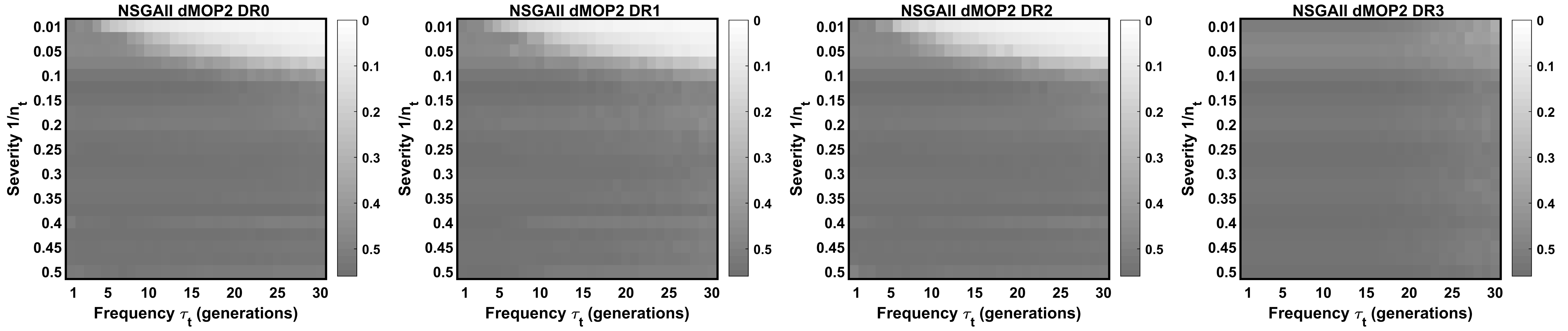
Figure 1. Frequency and severity heatmaps of HVD on dMOP2 for each response type (DR0: none, DR1: random solution addition, DR2: mutated solution addition, DR3: random restart). A zero-value shows optimal hypervolume attainment and higher values show poorer performance.

Figure 2. Frequency and severity heatmaps of HVD on HE1 for each algorithm and each response type (DR0: none, DR1: random solution addition, DR2: mutated solution addition, DR3: random restart). A zero-value shows optimal hypervolume attainment, higher values show poorer performance.

4. Results

Given that a limited range of parameters for the change severity and change frequency are investigated in the literature, the following results highlight the difficulty of the most popularly used change severity and frequency instances in terms of their ability to be solved by generic MOEAs.

We recognise that problems have different difficulty in spite of dynamics and by showing only select problems we narrow our conclusions. However, we aim to determine a sensible range of dynamic parameters for the presented DMOP benchmarks and provide a methodology such that the performance of newly devised algorithms is tested in a meaningful way. Moreover, we provide insights on baseline algorithm comparison and selecting dynamics parameters that novel algorithms should be tested on to show a meaningful development and contribution to the field.

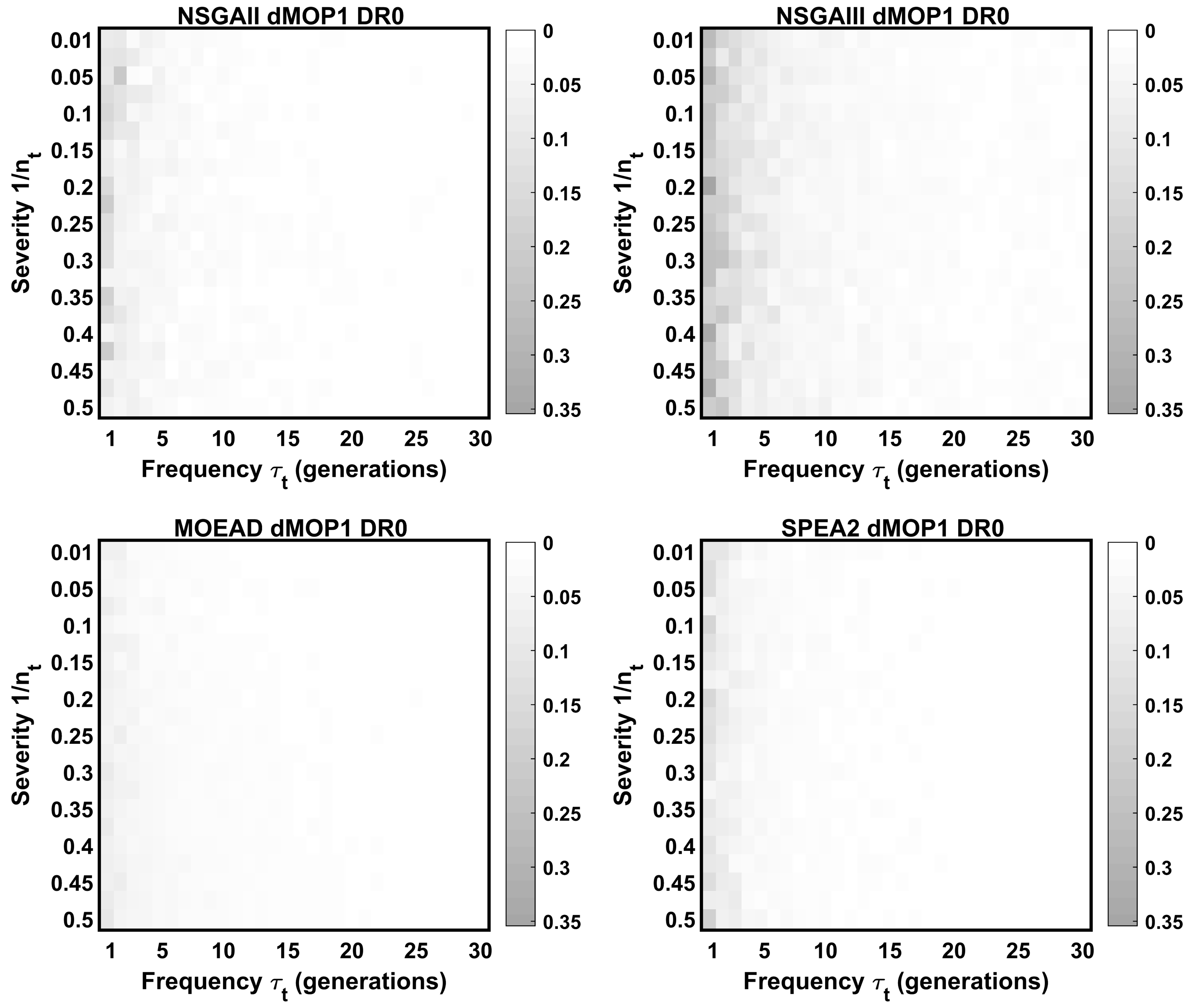
Figure 3. Heatmaps of HVD on the dMOP1 benchmark for each algorithm with no dynamic response mechanism. A zero-value shows complete attainment of optimal hypervolume. Combinations of frequency (x-axis) and severity (y-axis) are examined in ranges that include the commonly used values in the literature. Each cell represents the mean of 30x5 change events (150 pre-change-event measurements).

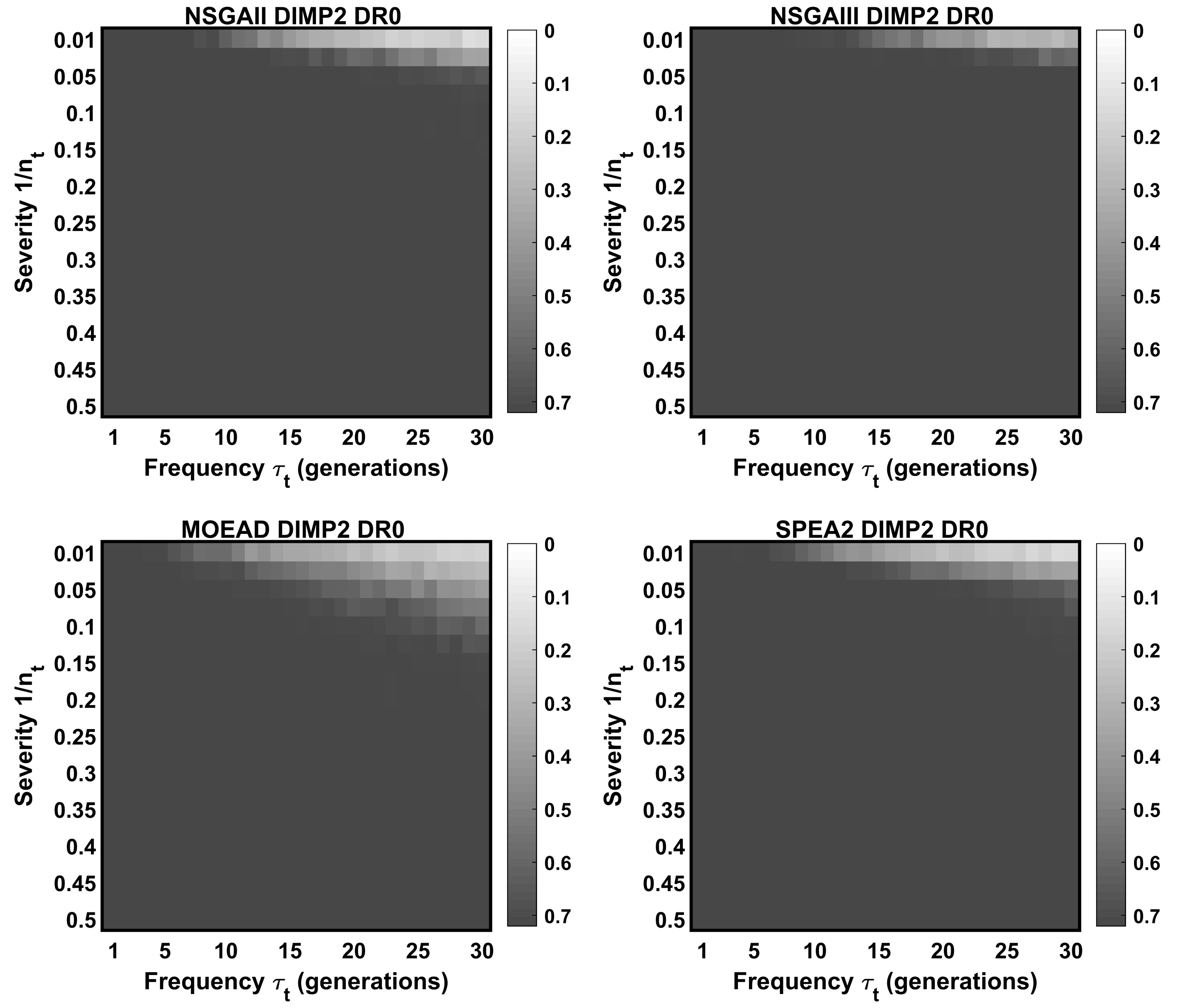
Figure 4. Heatmaps of HVD for the DIMP2 benchmark for each algorithm with no dynamic response mechanism. A zero-value shows complete attainment of optimal hypervolume. Combinations of frequency (x-axis) and severity (y-axis) are examined in ranges that include the commonly used values in the literature. Each cell represents the mean of 30x5 change events (150 pre-change-event measurements).

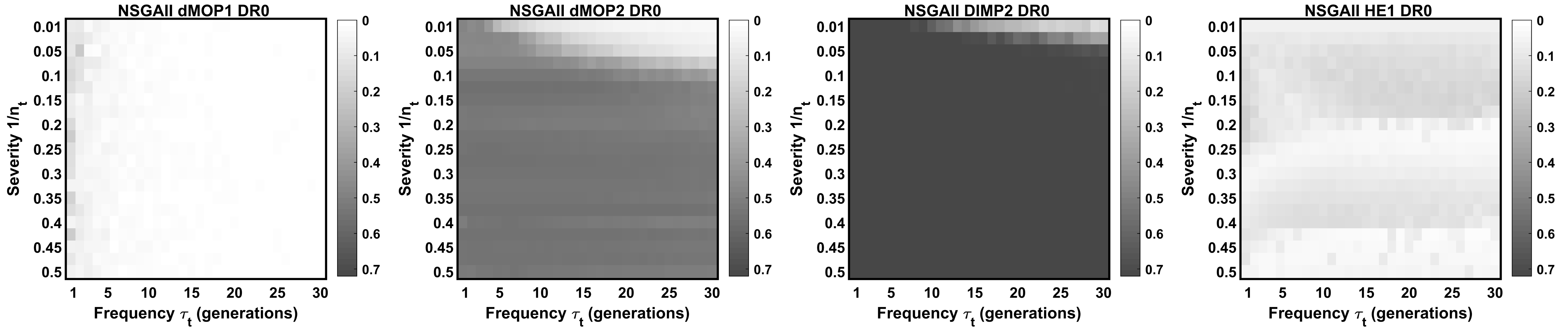
Figure 5. Frequency and severity heatmaps of HVD for the NSGA-II algorithm with no dynamic response mechanism on problems with Type I(DIMP2), II (dMOP2) and III (dMOP1/HE1) dynamics. A zero-value shows complete attainment of optimal hypervolume, higher values indicated poorer performance. Each cell represents the mean of 30x5 change events (150 pre-change-event measurements).

4.1. Justifying baseline dynamic responses for comparison

The ‘random restart’ mechanism is used in conjunction with a simple MOEA as a baseline for comparison in many papers that propose novel dynamic algorithms, however we demonstrate here through the hypervolume attainment, that it is not useful to use such a method for comparison. Figure 1, illustrates that of the considered simple baseline responses investigated here, restarting the algorithm (DR3 subplot) is clearly the worst. The hypervolume attainment is poor across the range of change severity values and frequencies compared with no response (DR0), and the random (DR1) and mutated (DR2) solution responses. Furthermore, little improvement is seen by purely addition of 20% mutated or randomised solutions; the DIMP2 problem appears difficult with literature-standard dynamics parameters for non-dynamic MOEAs. Figure 2 illustrates the performance of each response type in each algorithm for the HE1 problem. There is a more complex pattern of hypervolume attainment in the parameter space, with two bands of better performance at high severity ($\frac{1}{n_{t}}=0.5$) and mid-severity ($\frac{1}{n_{t}}=0.25$), but immediately worse performance vertically adjacent to these regions at ($\frac{1}{n_{t}}=0.4$) and ($\frac{1}{n_{t}}=0.2$). These patterns are consistent across the DR0, DR1 & DR2 response for the NSGA-II, NSGA-III & SPEA2 algorithms. The performance of MOEA/D algorithm is more homogeneous across the parameter combinations with these patterns less clearly defined. One possibility for this is the drastic and non-uniform change in POF shape the problem experiences with changing values of $t$. The non-uniform performance patterning means that for some values of the severity parameter, these specific successive changes in the problem’s POF are more easily handled. This implies that the $n_{t}$ parameter does not, for all problems, correspond to a series of change events of equal magnitude in terms of their difficulty for algorithms. This reinforces the need for careful selection of severity and frequency parameter values when benchmarking algorithms on DMOPs. All algorithms performance with the random restart response are also shown in the right most column of the grid in Figure 2. The negative impacts on algorithm performance are less severe at lower change frequencies ($\tau_{t}=30$), however the hypervolume difference remains high when compared with the other response types, as in Figure 1. This strengthens the evidence against using random restart in algorithms as a baseline for performance comparison.

4.2. Determining baseline parameters for dynamics in DMOPs

Figure 3 illustrates a key motivation of this work in providing insights into the capability of MOEA performance on DMOPs with commonly used values for the frequency and severity of changes. The dMOP1 problem poses little difficulty at any of the severity or frequency settings, with the exception of a change frequency of 1, where it can be expected that a generic algorithm might lose performance. Change severity had little impact, whilst smaller frequencies (more rapid changes) somewhat reduced the hypervolume attainment of the algorithms. Notably, this performance degradation occurs sooner for NSGA-III than for NSGA-II or the other algorithms. Our recommendation for dMOP1 is that most of the studied dynamics ranges in the literature can be effectively handled by generic MEOAs and therefore should not be used to test more complex novel dynamic algorithms.

Conversely, the DIMP2 problem poses a challenge to all the algorithms across most of the severity and frequency ranges. Figure 4 illustrates that for all algorithms, it is only for small severity and the least rapid changes that minimal HVD is possible, with MOEA/D having the best performance area. For the majority of the parameter ranges these generic DMOEAs cannot provide good results. Therefore our recommendation is that DIMP2 is suitable for benchmarking novel dynamic methods.

4.3. Algorithm performance on different dynamics types

We illustrate the variable performance of the NSGA-II algorithm on the problem subset in Figure 5. The difference in performance of a single algorithm on multiple problems is to be expected, however, more importantly these heatmaps illustrate the impact of dynamic parameter choices. Using the same values of change severity and frequency for different problems without justification can weaken conclusions on algorithm performance. For example, the NSGA-II algorithm, not designed for DMOPs, provides competitive performance on dMOP1 across all but the lowest frequency changes. Comparison of a novel DMOEA on this problem is effectively meaningless, other than to ensure a basic capability. Other existing DMOP benchmarks however, pose significant challenges for the examined MOEAs. For example, NSGA-II struggles on DIMP2 for most combinations of $n_{t}$ and $\tau_{t}$. It is these problems that should therefore be the focus when testing the efficacy of novel DMOEA constructions.

Furthermore, our results stress the importance of both selecting the parameters of the frequency and severity of changes and determining their importance in a problem’s difficulty. Concluding the effectiveness of a novel dynamic method on, for example, the dMOP2 problem with $n_{t}=20$ and $\tau_{t}=25$ is misleading. This combination of dynamic frequency and severity can effectively be handled by a generic MOEA.

4.4. Recommendations for Future Investigations

For each of the examined problems, we provide a summary of the minimum parameters we recommend to ensure a challenging problem set when evaluating algorithms.

dMOP1 - This problem did not provide a challenge for any of the MOEAs tested. A drop off in performance occurs when the change frequency $\tau_{t}=1$, however this would also be challenging for most DMOEAs except those specifically designed for problems with rapid changes. Our recommendation is therefore to avoid this problem except for ensuring fundamental capability compared to the MOEAs.

dMOP2 - The results on this problem indicate it is a good candidate for evaluating DMOEAs since the majority of the parameter space cannot effectively be handled by the MOEAs. Reciprocal severity values of at least $\frac{1}{n_{t}}=0.05$ are recommended in conjunction with most change frequencies. If $\tau_{t}$ is less than 15, smaller severity values can be considered.

DIMP2 - This problem was the most challenging for the MOEAs of the problems examined. Using $\frac{1}{n_{t}}=0.01$ was challenging at frequencies below 20 generations, and at all frequencies for greater severity values. The MOEA/D algorithm achieved slightly better performance at low frequencies (slower changes) and low severity values, however the overall HVD is poor.

HE1 - The results indicate a complex range of performance across the frequency and severity parameter space, perhaps due to the complex PF shape this problem has and the change that happens with different intervals of $t$. Careful selection of parameters may allow challenging instances, however the HV attainment is good for the MOEAs generally and therefore other problems may be better to evaluate DMOEAs.

We have evaluated the simplest modifications to MOEAs that are often used as baseline comparisons when evaluating novel DMOEAs. The results show that the commonly used ‘random restart’ response, where the entire population is re-initialized at every change event provides poor performance across the examined parameter space. In terms of function evaluations, an equivalent number would be used in a ‘do nothing’ approach, the DR0 response here. We therefore recommend that the random restart responses should not be used in conjunction with the examined parameter ranges. If there is justification that re-initialization may be beneficial, for example on problems with deceptive, multi-modal or many local optima, it should not be the only baseline considered - a passive approach may provide better results in many cases.

For the examined algorithms, the passive approach (DR0), the mutated solution addition (DR1), random solution addition (DR2) have relatively similar impacts on the HVD measurements, even on the HE1 problem which had a more complex performance pattern across the dynamic parameter space (as in Figure 2)

Ultimately, we echo the statements of many when we conclude that a diverse set of benchmarks should be used to examine algorithm performance (Helbig and Engelbrecht, 2013a; Raquel and Yao, 2013; Nguyen et al., 2012; Azzouz et al., 2016). However we build on this to include that the parameters governing the frequency and severity of changes must be carefully selected such that the resulting instances are sufficiently challenging and cannot be handled by static MOEAs.

5. Conclusion

Within this work, we have demonstrated the range of change frequency and severity parameter usage in the literature is unguided and for some dynamic multi-objective benchmarks does not result in challenging instances. Understanding the impacts of the parameters that control the dynamics in a set of selected benchmarks used to evaluate novel algorithms should be an important consideration in future works. Secondly we have evaluated the maximal performance of typical MOEAs not designed for DMOPs within the frequency and severity parameter range to provide an experimental schema to find recommendations for challenging instances that novel DMOEAs should consider in order to provide meaningful improvement. Our results elucidate the utility of different commonly used simple modifications to MOEAs in the literature which are often used as a baseline comparison for a proposed algorithm. We highlight the minimal impact on the considered subset of problems that mutated and random solutions provide and condemn the usage of the random restart response without valid justification. Finally, we share the DPTP with which we produced these results and declare the intention to expand upon its capability in terms of the scope of DMOPs and dynamic algorithms. Our motivation is to make experimentation on DMOPs more streamlined, reproducible and verifiable to facilitate comparison such that progress towards more effective algorithms and more challenging problems can occur.

References

- (1)
- Azzouz et al. (2016) Radhia Azzouz, Slim Bechikh, and Lamjed Ben Said. 2016. Dynamic multi-objective optimization using evolutionary algorithms: a survey. 31–70.
- Azzouz et al. (2017) Radhia Azzouz, Slim Bechikh, and Lamjed Ben Said. 2017. A dynamic multi-objective evolutionary algorithm using a change severity-based adaptive population management strategy. Soft Computing 21, 4 (2017), 885–906.
- Biswas et al. (2014) Subhodip Biswas, Swagatam Das, Ponnuthurai N. Suganthan, and Carlos A Coello Coello. 2014. Evolutionary Multi-Objective Optimization in dynamic environments:a set of benchmarks. Proc.2014 IEEE Congress on Evolutionary Computation 1 (2014), 74–88.
- Branke (1999) Jürgen Branke. 1999. Memory enhanced evolutionary algorithms for changing optimization problems. Proceedings of the 1999 Congress on Evolutionary Computation, CEC 1999 3, 721 (1999), 1875–1882. https://doi.org/10.1109/CEC.1999.785502
- Branke (2002) J. Branke. 2002. Evolutionary optimization in dynamic environments. Vol. 1.
- Branke and Schmeck (2003) Jürgen Branke and Hartmut Schmeck. 2003. Designing Evolutionary Algorithms for Dynamic Optimization Problems. (2003), 239–262.
- Cámara et al. (2009) Mario Cámara, Julio Ortega, and Francisco De Toro. 2009. Performance measures for dynamic multi-objective optimization. Lecture Notes in Computer Science (including subseries Lecture Notes in Artificial Intelligence and Lecture Notes in Bioinformatics) 5517 LNCS, PART 1 (2009), 760–767.
- Chen et al. (2018) Renzhi Chen, Ke Li, and Xin Yao. 2018. Dynamic Multiobjectives Optimization with a Changing Number of Objectives. IEEE Transactions on Evolutionary Computation 22, 1 (2018), 157–171. https://doi.org/10.1109/TEVC.2017.2669638 arXiv:1608.06514
- Deb and Jain (2014) Kalyanmoy Deb and Himanshu Jain. 2014. An Evolutionary Many-Objective Optimization Algorithm Using Reference-Point-Based Nondominated Sorting Approach, Part I: Solving Problems With Box Constraints. IEEE Transactions on Evolutionary Computation 18, 4 (2014), 577–601. https://doi.org/10.1109/TEVC.2013.2281535
- Deb et al. (2002) Kalyanmoy Deb, Amrit Pratap, Sameer Agarwal, and T. Meyarivan. 2002. A fast and elitist multiobjective genetic algorithm: NSGA-II. IEEE Transactions on Evolutionary Computation 6, 2 (2002), 182–197.
- Deb et al. (2007) Kalyanmoy Deb, N Udaya Bhaskara Rao, and Sindhya Karthik. 2007. Dynamic Multi-Objective Optimization and Decision-Making Using Modified NSGA-II: A Case Study on Hydro-Thermal Power Scheduling. EMO’07 Proceedings of the 4th international conference on Evolutionary multi-criterion optimization (2007), 803–817.
- Farina et al. (2003) M Farina, K Deb, and P Amato. 2003. Dynamic Multiobjective Optimization Problems: Test Cases Approximation and Applications. Evolutionary Multi-Criterion Optimization. Second International Conference EMO 2003 8, 5 (2003), 311–326.
- Gee et al. (2017) Sen Bong Gee, Kay Chen Tan, and Hussein A. Abbass. 2017. A Benchmark Test Suite for Dynamic Evolutionary Multiobjective Optimization. IEEE Transactions on Cybernetics 47, 2 (2017), 461–472. https://doi.org/10.1109/TCYB.2016.2519450
- Goh and Tan (2009) Chi Keong Goh and Key Chen Tan. 2009. A competitive-cooperative coevolutionary paradigm for dynamic multiobjective optimization. IEEE Transactions on Evolutionary Computation 13, 1 (2009), 103–127. https://doi.org/10.1109/TEVC.2008.920671
- Hasan et al. (2019) Md Mahmudul Hasan, Khin Lwin, Maryam Imani, Antesar Shabut, Luiz Fernando Bittencourt, and M. A. Hossain. 2019. Dynamic multi-objective optimisation using deep reinforcement learning: benchmark, algorithm and an application to identify vulnerable zones based on water quality. Engineering Applications of Artificial Intelligence 86, 2013 (2019), 107–135. https://doi.org/10.1016/j.engappai.2019.08.014
- Hatzakis and Wallace (2006) Iason Hatzakis and David Wallace. 2006. Dynamic multi-objective optimization evolutionary algorithms: a Forward-Looking approach. Proceedings of ACM GECCO 4 (2006), 1201–1208.
- Helbig and Engelbrecht (2013a) Marde Helbig and Andries P. Engelbrecht. 2013a. Benchmarks for dynamic multi-objective optimisation. Proceedings of the 2013 IEEE Symposium on Computational Intelligence in Dynamic and Uncertain Environments, CIDUE 2013 - 2013 IEEE Symposium Series on Computational Intelligence, SSCI 2013 46, 3 (2013), 84–91.
- Helbig and Engelbrecht (2013b) Mardé Helbig and Andries P. Engelbrecht. 2013b. Performance measures for dynamic multi-objective optimisation algorithms. Information Sciences 250 (2013), 61–81.
- Huang et al. (2011) Liang Huang, Il Hong Suh, and Ajith Abraham. 2011. Dynamic multi-objective optimization based on membrane computing for control of time-varying unstable plants. Information Sciences 181, 11 (2011), 2370–2391. https://doi.org/10.1016/j.ins.2010.12.015
- Jiang et al. (2019) Shouyong Jiang, Marcus Kaiser, Shengxiang Yang, Stefanos Kollias, and Natalio Krasnogor. 2019. A Scalable Test Suite for Continuous Dynamic Multiobjective Optimization. IEEE Transactions on Cybernetics (2019), 1–13. https://doi.org/10.1109/tcyb.2019.2896021 arXiv:arXiv:1903.02510v1
- Jiang and Yang (2014) Shouyong Jiang and Shengxiang Yang. 2014. A Benchmark Generator for Dynamic Optimization. Proceedings of the 2014 UK Workshop on Computational IntelligenceAt: University of Bradford, UK (2014).
- Jiang and Yang (2017) Shouyong Jiang and Shengxiang Yang. 2017. Evolutionary Dynamic Multiobjective Optimization: Benchmarks and Algorithm Comparisons. IEEE Transactions on Cybernetics 47, 1 (2017), 198–211.
- Jiang et al. (2018) Shouyong Jiang, Shengxiang Yang, Xin Yao, Kay Chen Tan, and Marcus Kaiser. 2018. Benchmark Problems for CEC2018 Competition on Dynamic Multiobjective Optimisation. CEC2018 Competition (2018), 1–18.
- Koo et al. (2010) Wee Tat Koo, Chi Keong Goh, and Kay Chen Tan. 2010. A predictive gradient strategy for multiobjective evolutionary algorithms in a fast changing environment. Memetic Computing 2, 2 (2010), 87–110. https://doi.org/10.1007/s12293-009-0026-7
- Mehnen et al. (2006) J. Mehnen, Tobias Wagner, and G. Rudolph. 2006. Evolutionary Optimization of Dynamic Multiobjective Functions. Technical Report CI-204/06 Dortmund University (2006).
- Morrison (2013) R.W. Morrison. 2013. Designing Evolutionary Algorithms for Dynamic Environments. Springer Berlin Heidelberg.
- Muruganantham et al. (2016) Arrchana Muruganantham, Kay Chen Tan, and Prahlad Vadakkepat. 2016. Evolutionary Dynamic Multiobjective Optimization Via Kalman Filter Prediction. IEEE Transactions on Cybernetics 46, 12 (2016), 2862–2873.
- Nguyen et al. (2012) T.T. Nguyen, S. Yang, and J. Branke. 2012. Evolutionary dynamic optimization: A survey of the state of the art. Swarm and Evolutionary Computation 6 (2012).
- Peng et al. (2013) Xingguang Peng, Shengxiang Yang, Demin Xu, and Xiaoguang Gao. 2013. Evolutionary Algorithms for theMultiple Unmanned Aerial Combat Vehicles Anti-ground Attack Problem in Dynamic Environments. 490 (2013), 403–431. https://doi.org/10.1007/978-3-642-38416-5
- Raquel and Yao (2013) Carlo Raquel and Xin Yao. 2013. Dynamic Multi-objective Optimization: A Survey of the State-of-the-Art. 85–106.
- Rohlfshagen et al. (2009) Philipp Rohlfshagen, Per Kristian Lehre, and Xin Yao. 2009. Dynamic evolutionary optimisation: an analysis of frequency and magnitude of change. Proceedings of the 11th Annual conference on Genetic and evolutionary computation (GECCO2009) (2009), 1713–1720. https://doi.org/10.1145/1569901.1570131
- Ruan et al. (2021) Gan Ruan, Jinhua Zheng, Juan Zou, Zhongwei Ma, and Shengxiang Yang. 2021. A random benchmark suite and a new reaction strategy in dynamic multiobjective optimization. Swarm and Evolutionary Computation 63, December 2020 (2021), 100867. https://doi.org/10.1016/j.swevo.2021.100867
- Tang et al. (2007) Min Tang, Zhangcan Huang, and Guangxi Chen. 2007. The Construction of Dynamic Multi-objective Optimization Test Functions. Advances in Computation and Intelligence. Second International Symposium (ISICA’2007) (2007), 72–79.
- Tian et al. (2017) Ye Tian, Ran Cheng, Xingyi Zhang, and Yaochu Jin. 2017. PlatEMO: A MATLAB Platform for Evolutionary Multi-Objective Optimization. IEEE Computational Intelligence Magazine 12, 4 (2017), 73 – 87.
- Yang (2003) Shengxiang Yang. 2003. Non-stationary problem optimization using the primal-dual genetic algorithm. In The 2003 Congress on Evolutionary Computation, 2003. CEC ’03., Vol. 3. 2246–2253 Vol.3. https://doi.org/10.1109/CEC.2003.1299951
- Yazdani et al. (2020) Danial Yazdani, Mohammad Nabi Omidvar, Ran Cheng, Jürgen Branke, Trung Thanh Nguyen, and Xin Yao. 2020. Benchmarking Continuous Dynamic Optimization: Survey and Generalized Test Suite. IEEE Transactions on Cybernetics (2020).
- Zhang et al. (2021b) Haijuan Zhang, Gai Ge Wang, Junyu Dong, and Amir H. Gandomi. 2021b. Improved nsga‐iii with second‐order difference random strategy for dynamic multi‐objective optimization. Processes 9, 6 (2021), 1–23. https://doi.org/10.3390/pr9060911
- Zhang et al. (2021a) Qingyang Zhang, Shouyong Jiang, Shengxiang Yang, and Hui Song. 2021a. Solving dynamic multi-objective problems with a new prediction-based optimization algorithm. Vol. 16. 1–39 pages. https://doi.org/10.1371/journal.pone.0254839
- Zhang and Li (2008) Qingfu Zhang and Hui Li. 2008. MOEA/D: A Multiobjective Evolutionary Algorithm Based on Decomposition. Evolutionary Computation, IEEE Transactions on 11 (01 2008), 712 – 731. https://doi.org/10.1109/TEVC.2007.892759
- Zhou et al. (2014) Aimin Zhou, Yaochu Jin, and Qingfu Zhang. 2014. A Population prediction strategy for evolutionary dynamic multiobjective optimization. IEEE Transactions on Cybernetics 44, 1 (2014), 40–53.
- Zhou et al. (2007) Aimin Zhou, Yaochu Jin, Qingfu Zhang, Bernhard Sendhoff, and Edward Tsang. 2007. Prediction-Based Population Re-initialization for Evolutionary Dynamic Multi-objective Optimization. Proceedings of EMO,LNCS4403 (2007), 832–846.
- Zitzler et al. (2002) Eckart Zitzler, Marco Laumanns, and Lothar Thiele. 2002. SPEA2: Improving the Strength Pareto Evolutionary Algorithm For Multiobjective Optimization. Tehcnical Report.
- Zou et al. (2021) Fei Zou, Gary G. Yen, and Chen Zhao. 2021. Dynamic multiobjective optimization driven by inverse reinforcement learning. Information Sciences 575 (2021), 468–484. https://doi.org/10.1016/j.ins.2021.06.054