The MeerTime Pulsar Timing Array –
A Census of Emission Properties and Timing Potential

Abstract

MeerTime is a five-year Large Survey Project to time pulsars with MeerKAT, the 64-dish South African precursor to the Square Kilometre Array. The science goals for the programme include timing millisecond pulsars to high precision ($<1\,\upmu$s) to study the Galactic MSP population and to contribute to global efforts to detect nanohertz gravitational waves with the International Pulsar Timing Array (IPTA). In order to plan for the remainder of the programme and to use the allocated time most efficiently, we have conducted an initial census with the MeerKAT “L-band” receiver of 189 MSPs visible to MeerKAT and here present their dispersion measures, polarization profiles, polarization fractions, rotation measures, flux density measurements, spectral indices, and timing potential. As all of these observations are taken with the same instrument (which uses coherent dedispersion, interferometric polarization calibration techniques, and a uniform flux scale), they present an excellent resource for population studies. We used wideband pulse portraits as timing standards for each MSP and demonstrated that the MeerTime Pulsar Timing Array (MPTA) can already contribute significantly to the IPTA as it currently achieves better than 1 $\upmu$s timing accuracy on 89 MSPs (observed with fortnightly cadence). By the conclusion of the initial five-year MeerTime programme in July 2024, the MPTA will be extremely significant in global efforts to detect the gravitational wave background with a contribution to the detection statistic comparable to other long-standing timing programmes.

1 Introduction

Millisecond pulsars (MSPs) are the sub-population of pulsars that are characterised by short spin periods ($P<50$ ms) and low magnetic field strengths ($B_{\textrm{surf}}<10^{10}$ G). The first binary pulsar, PSR B1913$+$16 (J1915$+$1606; Hulse & Taylor 1975), possessed an unusually low spin period ($P=59$ ms) and magnetic field strength ($B_{\textrm{surf}}=2\times 10^{10}\,$G) compared to the bulk of the population known at the time, which, apart from the young Crab and Vela pulsars, consisted mainly of solitary pulsars with spin periods of typically 0.1-2 s and magnetic fields of order 10¹² G. Prior to the discovery of PSR B1913+16, Bisnovatyi-Kogan & Komberg (1974) had predicted that mass accretion onto neutron stars may decrease their magnetic fields, and PSR B1913+16 appeared to agree with their prediction as at least one of the NSs in this system must have accreted matter during a previous stage of mass transfer. When the first MSP, PSR B1937+21 (J1939+2134), was discovered with $P=1.56$ ms and $B_{\textrm{surf}}=4\times 10^{8}$ G (Backer et al., 1982), it was soon proposed that a (now missing) companion had been responsible for its spin-up and the low field made spin-up to its millisecond period possible (Alpar et al., 1982; Radhakrishnan & Srinivasan, 1982). As more recycled pulsars were discovered, a self-consistent model began to emerge (e.g., Bailes, 1989) in which most pulsars lost their binary companions in the initial explosion due to impulsive kicks and mass loss at the time of the first explosion, but those that remained bound had a chance for a second life upon accreting material from their evolved companions that not only reduced their magnetic field strengths but made it possible for them to be spun-up to millisecond periods. NSs with lower-mass companions accrete material for longer than those with high-mass companions because their evolutionary timescales are longer, and they are able to be spun up to very short periods ($P\sim 1.5$ ms) with an associated reduction of their magnetic fields to $\sim 10^{8}$ G. MSPs with heavier white dwarf companions tend to spin more slowly ($P\sim 10$ - $16$ ms) with some notable exceptions, such as PSR J1614$-$2230 (Crawford et al., 2006; Demorest et al., 2010), and those with NS companions slower still ($P\sim 16$ - $60$ ms). For an early paper describing these models, see Bhattacharya & van den Heuvel (1991), and, for a more recent discussion of their binary properties, Tauris et al. (2017). Support for these models (see, e.g., Phinney, 1992) comes in part from the large fraction of MSPs observed to have binary companions compared to the fraction of “normal” pulsars in binaries ($\sim 74$% of MSPs are in binaries but only $\sim 2$% of longer-period pulsars are in binaries; from the Australia Telescope National Facility (ATNF) Pulsar Catalogue, v.1.64, Manchester et al. 2005).

Studies of the properties of MSPs and the Galactic MSP population overall have often been limited or biased by small sample sizes (e.g., Johnston & Bailes, 1991) or by instrumentation that prohibits studies of the polarization or novel features of the pulse profile, which are probably determined by the pulsar’s magnetosphere and spin period. See, for example, Kramer et al. (1998), Xilouris et al. (1998), and Kramer et al. (1999) for a comprehensive study of 27 MSPs, or the review by Kramer & Xilouris (2000), and references therein. The majority of MSPs have been discovered by quasi-uniform surveys by large-aperture telescopes such as the Parkes 64-m radio telescope (also known as Murriyang; e.g., Manchester et al. 2001; Keith et al. 2010), the Arecibo 305-m dish (e.g., Cordes et al., 2006), and the Green Bank 100-m Telescope (GBT; e.g., Boyles et al. 2013; Stovall et al. 2014). More recently, other instruments like the Low-Frequency Array (LOFAR) and Giant Metrewave Radio Telescope (GMRT) have discovered pulsars in a combination of quasi-uniform surveys and targeted observations of gamma-ray point sources with pulsar characteristics (see, e.g., Ray et al., 2012; Bhattacharyya et al., 2016; Sanidas et al., 2019). In many cases, the only published pulse profiles are those formed using survey data and thus limited in resolution due to survey data rates as well as the use of incoherent dispersion correction. It is not uncommon for pulsars with large dispersion measures to have narrow features smeared beyond recognition using the discovery hardware which cannot a priori know the DM of the pulsars.

There is also some inconsistency in reported MSP flux densities in the ATNF Pulsar Catalogue and the literature. This is for a variety of reasons that include uncertainties in the pulsar position within the primary beam during initial timing, pulsar scintillation that makes pulsars more likely to have been brighter in their discovery observations, and design limitations that make absolute flux calibration a secondary consideration in the construction of some pulsar survey hardware. For example, the flux density of PSR J1843$-$1113 was first determined by Hobbs et al. (2004) to be $S_{1400}=0.1$ mJy, but was revised to 0.3 mJy by Levin et al. (2013), and then to 0.6 mJy by Desvignes et al. (2016).

Analyses of MSP polarization profiles and their evolution with radio frequency, which could potentially lead to a more consistent theory of the pulsar emission mechanism, have only been performed on samples of a few to $\sim 20$ MSPs (e.g., Rankin et al., 2017, and references therein), and the field could significantly benefit from a large comprehensive analysis derived from high signal-to-noise ratio ($S/N$) observations. Additional areas of pulsar astronomy that would benefit from such a dataset include probing the Galactic magnetic field with rotation measure (RM) measurements (e.g., Han et al., 2018; Sobey et al., 2019), improving Galactic electron density models with new independent distance measurements (see, e.g., Matthews et al., 2016; Yao et al., 2017), and constraining models of the NS equation of state through MSP mass measurements (Özel & Freire, 2016).

Estimates of the total MSP (Levin et al., 2013) and binary NS-NS populations (e.g., Burgay et al., 2003) rely upon our understanding of the MSP luminosity function, which in turn depends upon measured MSP distances, flux densities and their pulse shapes. Hence an authoritative survey of MSPs with the same flux density scale, coherent dedispersion to ascertain the true pulse shape, and ultimately pulsar parallaxes from timing is very valuable when we want to estimate their underlying populations and ascertain potential yields for future pulsar surveys and timing programmes such as those planned for the Square Kilometre Array (SKA; e.g., Levin et al., 2018).

The new precursor to the Square Kilometre Array (SKA) in South Africa, MeerKAT (Meer Karoo Array Telescope), presents an opportunity to revisit the fluxes, spectral indices, pulse shapes, polarimetry, and timing potential of the MSPs visible to it. The MeerTime project (Bailes et al., 2020) is a MeerKAT Large Survey Project and has four major themes. These include the Thousand Pulsar Array (Johnston et al., 2020), the Relativistic Binary programme (Kramer et al., 2021), the Globular Cluster pulsar timing programme (Ridolfi et al., 2021), and the MPTA, which studies MSPs with the primary aim of detecting gravitational waves. Parthasarathy et al. (2021) analysed the pulse-to-pulse variability (“jitter”) of 29 of these MSPs, placing limits on their timing precision. In this work, we present a census of 189 MSPs visible to MeerKAT at $\sim 1400$ MHz frequencies, providing high-time-resolution, polarization- and flux-calibrated profiles, measured DMs, polarization fractions, RMs, sub-banded flux densities, and spectral indices, as well as timing potential for the MPTA. The first results of the MPTA will be presented by Miles et al. (2022, in prep.), including a full release of timing residuals and refined ephemerides, and closely followed by an analysis of red noise and GW search (Middleton et al., 2022, in prep..

The 64 13.5-m offset Gregorian MeerKAT dishes have a high aperture efficiency and low system temperature that achieves a system equivalent flux density of just $\approx 7.0$  Jy at $\sim 1400$ MHz frequencies with the full array (Jonas & MeerKAT Team, 2016). With an antenna gain roughly 4 times that of Parkes, a lower system temperature ($\sim 18$ K), and a larger bandwidth (856 MHz of the MeerKAT L-band receiver compared with the 340 MHz of the Parkes multibeam receiver that was used for much of the last decade for the Parkes Pulsar Timing Array (PPTA; Manchester et al., 2013)), MeerKAT has become the best telescope in the southern hemisphere for a large-scale MSP observing programme and population study (Bailes et al., 2020). Compared to, for example, the Five-hundred-meter Aperture Synthesis Telescope (FAST), which can observe down to Dec $>-15$ degrees, MeerKAT has a lower sensitivity but greater sky coverage (Dec $<+40$ degrees, which includes the MSP-rich Galactic centre) and significantly higher slew rates (60 and 120 deg min^-1 in elevation and azimuth respectively). The 500-m diameter FAST has much superior gain but can only observe about one source every ten minutes due to reconfiguration overheads. The ability to quickly move between sources with minimal overhead is one of the advantages of large-N (number), small-D (diameter) arrays like MeerKAT.

The timing precision and stability of MSPs can additionally be leveraged to search for low-frequency GWs through observations of arrays of MSPs like a galactic-scale interferometer, termed Pulsar Timing Arrays (PTAs; Hellings & Downs, 1983). The current global effort, the IPTA, places stringent constraints on the amplitude of a GW background but no detection has been made (Perera et al., 2019), although there are tantalising indications of similar spectral slopes in the red noise of the timing residuals of many of the MSPs with no spatial correlations indicative of a GW background (e.g., Arzoumanian et al., 2020; Chen et al., 2021; Goncharov et al., 2021). While the sensitivity of current Pulsar Timing Arrays to a GW signal scales favourably with time, it can be greatly accelerated by adding more pulsars to the array and increasing the cadence (Siemens et al., 2013). As Parkes is the largest telescope in the southern hemisphere currently contributing to PTA efforts, MeerTime can contribute significantly to the IPTA by $i)$ observing the current IPTA pulsars with higher precision, $ii)$ observing additional pulsars not currently included in the IPTA due to low precision, and $iii)$ helping offset the recent loss of the Arecibo 305-m telescope.

Throughout this paper, we define MSPs as having rotational periods $<50$ ms and period derivatives $<2\times 10^{-17}$ s s^-1. In section 2, we discuss the sources included in this census and the observational parameters. We further discuss the polarization properties in section 3, the flux density measurements in section 4, and the preliminary timing results in section 5. We conclude with some predictions for the SKA in section 6. Information on accessing FITS-format files of integrated pulse profiles as well as the full table of results is provided at the end of this manuscript.

2 Methods

All observations included in this paper were performed with the MeerKAT L-band receiver (856-1712 MHz) with the Pulsar Timing User Supplied Equipement (PTUSE) back-end that uses coherent dedispersion. A full description of the observing system can be found in Bailes et al. (2020). Typical observations used 54-61 dishes resulting in a system equivalent flux density of 6.3-7.2 Jy near 1400 MHz. The system temperature varies as a function of frequency and is slightly worse near the band edges but difficult to measure in the areas of the band permanently affected by radio frequency interference (RFI) (Bailes et al., 2020; Geyer et al., 2021). While the MeerKAT Ultra-High Frequency (UHF) receiver at 544-1088 MHz is now fully commissioned for pulsar timing, time constraints did not allow for a full MSP census with the UHF receiver. Using the results of this L-band census, a smaller census of low-DM, steep-spectrum sources with the UHF receiver may be feasible, and such sources may be observed with the UHF receiver for the MPTA. The same applies for high-DM, flat-spectrum sources with the MeerKAT S-band receiver in future.

As the original network interface card for the first pulsar timing user supplied equipment (PTUSE) machine was unable to ingest the full bandwidth in “1K mode” (using 1024 channels across the 856-MHz band), observations between mid-April 2019 and February 2020 were restricted to 928 frequency channels (dropping 48 channels from the top and bottom of the band where the roll-off adversely affects sensitivity in any case), reducing the recorded bandwidth to 775.75 MHz. In order to maintain consistency throughout our analyses, we therefore chose to reduce the observations with 856 MHz of recorded bandwidth down to the same 775.75 MHz. The loss in sensitivity is nearly negligible because of the sharp roll-off at the edges of the receiver band; comparisons of $S/N$ measurements of a sample of 20 pulsars (250 observations) show a median sensitivity loss of only 2.2% (mean of 4.5%). Almost all of our pulsars have negative spectral indices (typically between $-$1 and $-$3), which makes the loss of the lower part of the band worse than the top of it. Broader bands also make determination of DMs more accurate, which in turn aids in precision timing. Since late Feb 2020, all of our observations have used the entire 856 MHz of bandwidth.

Our source list was derived from the ATNF pulsar catalogue (using v.1.63; Manchester et al., 2005), limited to radio-loud MSPs not associated with globular clusters and visible to MeerKAT (Dec $\leq+30$ degrees to avoid severe time restrictions). We further restricted the list to exclude sources with positional uncertainties greater than 2 arcsec (near the resolution of the tied array beam) or without complete timing solutions (ephemerides) available to us, and we removed 12 Northern sources (Dec $>0$ degrees) with known low flux densities ($S_{1400}<0.1$ mJy), under the assumption that these could be observed with greater efficiency by Northern telescopes and were unlikely to efficiently contribute to the timing array. Finally, some sources were removed from our list (after one or more initial observations) due to insufficient precision in ephemeris parameters (leading to significant “smearing” in individual 8-second sub-integrations) or due to low $S/N$ in 1024-second observations. In total, 33 sources were excluded from our original list. To this list, we added 4 unpublished sources (or sources with currently unpublished timing solutions) matching the same sample limits; these MSPs were discovered in the Einstein@Home reprocessing of the Parkes Multibeam Pulsar Survey (Knispel et al., 2013) and the Green Bank North Celestial Cap survey (Stovall et al., 2014). We list our sources with basic parameters, including number of observations, and references in Table 1, where the DMs indicated are fitted from the brightest epoch per source. We also plot the sources in a $P$-$\dot{P}$ diagram in Figure 1, where $P$ is the rotation period of the pulsar and the dot denotes its time derivative. We note that, although initial ephemerides from published sources, the ATNF pulsar catalogue, or private communication were used as a starting point, we regularly refined ephemerides to ensure high-quality observations. These updated ephemerides will be presented in future work (Miles et al., 2022, in prep.).

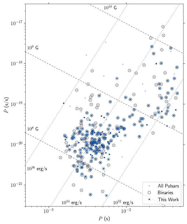
Figure 1: A $P$-$\dot{P}$ diagram showing the known MSPs (purple dots) and those included in the MeerTime MSP census project (blue dots). Binary MSPs are outlined with a circle. The data are from the ATNF pulsar catalogue v1.64 (Manchester et al., 2005).

Table 1: The 189 pulsars included in the MeerTime census with basic parameters, measured RMs with 1-$\sigma$ uncertainties, percentages of linear polarization ($L/I$), circular polarization ($V/I$) and absolute circular polarization ($|V|/I$), median ToA uncertainties normalised to 256 seconds (see section 5 for details), flux densities at 1400 MHz, spectral indices from the power law model fit, and references (initial publication). The number of observations included in the analysis for each pulsar is given in the second column. Values less than 1-$\sigma$ for constrained-positive parameters are given as 2-$\sigma$ upper limits. The pulsars included in the regular observing programme (88 out of the 89) are indicated with asterisks. RMs measured from summed observations (not the mean of RMs from multiple observations) are indicated with a dagger ($\dagger$).

Source Name	$N$	Period	DM	RM	$L/I$	$V/I$	$|V|/I$	Median ToA	$S_{1400}$	$\alpha$	Reference
								Uncertainty
		(ms)	(pc cm-3)	(rad m-2)	(%)	(%)	(%)	($\upmu$s)	(mJy)
J0023+0923	$6$	$3.05$	$14.3216(6)$	$-5.1(9)$	$30(2)$	$3(2)$	$3(2)$	$0.49$	$0.73(12)$	$-1.4(7)$	Hessels et al. 2011
J0030+0451∗	$33$	$4.87$	$4.33294(11)$	$1.32(13)$	$33(2)$	$0.9(22)$	$2(2)$	$0.91$	$1.09(3)$	$-2.4(2)$	Lommen et al. 2000
J0034$-$0534	$6$	$1.88$	$13.748(2)$	–†	$<4.1$	$-3(4)$	$<8.1$	$2.5$	$0.21(5)$	$-1.0(9)$	Bailes et al. 1994
J0101$-$6422∗	$8$	$2.57$	$11.9210(4)$	$20(10)$	$21(2)$	$2(6)$	$<11.2$	$2.0$	$0.156(11)$	$-1.4(5)$	Kerr et al. 2012
J0125$-$2327∗	$39$	$3.68$	$9.5974(3)$	$4.78(7)$	$34(2)$	$-3(2)$	$2(2)$	$0.19$	$2.49(12)$	$-1.0(2)$	McEwen et al. 2020
J0154+1833	$6$	$2.36$	$19.79830(14)$	$-21.9(6)$†	$30(2)$	$-0.7(61)$	$<12.1$	$0.89$	$0.11(2)$	$-1.7(8)$	Martinez et al. 2019
J0348+0432	$6$	$39.1$	$40.464(7)$	$48.3(3)$	$28(2)$	$-13(3)$	$11(3)$	$1.6$	$0.67(4)$	$-1.8(3)$	Lynch et al. 2013
J0407+1607	$6$	$25.7$	$35.593(6)$	–†	$4(2)$	$6(3)$	$5(3)$	$14$	$0.35(2)$	$-2.5(2)$	Lorimer et al. 2005
J0437$-$4715∗	$74$	$5.76$	$2.6411(2)$	$0.15(2)$	$25(2)$	$-5(3)$	$13(3)$	$0.0087$	$126(2)$	$-1.78(11)$	Johnston et al. 1993
J0453+1559	$6$	$45.8$	$30.298(2)$	$-35.3(3)$	$20(2)$	$-0.1(31)$	$<6.1$	$1.8$	$0.33(2)$	$-1.3(3)$	Deneva et al. 2013
J0509+0856	$6$	$4.06$	$38.3271(8)$	$44.1(3)$	$22(2)$	$2(2)$	$3(2)$	$1.6$	$1.47(3)$	$-2.19(9)$	Martinez et al. 2019
J0557+1550	$6$	$2.56$	$102.5700(12)$	$26(1)$	$27(2)$	$0(10)$	$<21$	$3.8$	$0.067(5)$	$-2.0(3)$	Scholz et al. 2015
J0557$-$2948	$6$	$43.6$	$49.033(2)$	$1(2)$	$17(2)$	$-2(9)$	$<18$	$5.6$	$0.046(2)$	$-2.2(2)$	Kawash et al. 2018
J0610$-$2100∗	$38$	$3.86$	$60.6865(3)$	$33.7(2)$	$71(2)$	$-5(2)$	$5(2)$	$0.78$	$0.65(2)$	$-1.24(14)$	Burgay et al. 2006
J0613$-$0200∗	$36$	$3.06$	$38.7750(5)$	$18.4(2)$	$19(2)$	$0.3(21)$	$3(2)$	$0.18$	$2.15(7)$	$-2.09(13)$	Lorimer et al. 1995
J0614$-$3329∗	$39$	$3.15$	$37.05245(14)$	$38.9(2)$	$31(2)$	$-1(2)$	$2(2)$	$0.52$	$0.68(4)$	$-1.7(2)$	Ransom et al. 2011
J0621+1002	$6$	$28.9$	$36.5533(7)$	$52.0(2)$	$21(2)$	$-16(2)$	$14(2)$	$1.1$	$1.72(14)$	$-2.4(3)$	Camilo et al. 1996
J0621+2514	$6$	$2.72$	$83.633(3)$	$11(2)$	$64(3)$	$10(10)$	$<27$	$11$	$0.079(3)$	$-1.5(2)$	Sanpa-arsa 2016
J0636$-$3044∗	$25$	$3.95$	$15.4589(4)$	$36.9(2)$	$41(2)$	$2(2)$	$6(2)$	$1.9$	$1.51(14)$	$-0.9(5)$	Morello et al. 2019
J0709+0458	$6$	$34.4$	$44.273(3)$	$42.0(6)$	$21(2)$	$4(3)$	$<6.9$	$4.3$	$0.256(7)$	$-1.52(11)$	Martinez et al. 2019
J0711$-$6830∗	$40$	$5.49$	$18.4096(2)$	$23.9(3)$	$15(2)$	$-15(2)$	$14(2)$	$0.76$	$2.6(3)$	$-1.7(4)$	Bailes et al. 1997
J0721$-$2038	$6$	$15.5$	$76.093(6)$	$-18.4(4)$	$27(2)$	$-18(4)$	$16(4)$	$5.7$	$0.273(6)$	$-1.72(9)$	Burgay et al. 2013a
J0732+2314	$6$	$4.09$	$44.670(3)$	$-3(2)$	$22(2)$	$18(3)$	$16(3)$	$5.9$	$0.73(8)$	$-1.3(5)$	Martinez et al. 2019
J0737$-$3039A	$10$	$22.5$	$48.916(2)$	$120.46(4)$	$33(2)$	$-0.9(20)$	$4(2)$	$1.1$	$3.06(7)$	$-1.86(13)$	Burgay et al. 2003
J0751+1807	$6$	$3.48$	$30.2409(6)$	$41.6(2)$	$27(2)$	$-10(2)$	$10(2)$	$0.50$	$1.35(6)$	$-1.1(2)$	Lundgren et al. 1995
J0824+0028	$6$	$9.86$	$34.5473(12)$	$38.7(3)$	$43(2)$	$6(4)$	$8(4)$	$3.4$	$0.51(2)$	$-2.20(14)$	Deneva et al. 2013
J0900$-$3144∗	$39$	$11.1$	$75.6862(7)$	$85.43(5)$	$38(2)$	$9(2)$	$10(2)$	$0.58$	$3.84(3)$	$-1.30(4)$	Burgay et al. 2006
J0921$-$5202	$8$	$9.68$	$122.710(3)$	$-179(1)$	$32(2)$	$3(7)$	$<14.2$	$8.3$	$0.189(7)$	$-1.6(2)$	Mickaliger et al. 2012
J0931$-$1902∗	$22$	$4.64$	$41.4900(5)$	$-100.2(2)$	$34(2)$	$1(2)$	$3(2)$	$0.96$	$0.52(4)$	$-2.4(3)$	Laffon et al. 2015
J0955$-$6150∗	$67$	$2.00$	$160.8997(2)$	$-49(1)$	$4(2)$	$0.5(21)$	$8(2)$	$1.0$	$0.639(12)$	$-3.18(8)$	Camilo et al. 2015
J1012$-$4235∗	$40$	$3.10$	$71.6515(3)$	$61.8(5)$	$20(2)$	$2(3)$	$4(3)$	$0.82$	$0.258(6)$	$-1.33(11)$	Camilo et al. 2015
J1017$-$7156∗	$53$	$2.34$	$94.21473(10)$	$-63.36(8)$	$38(2)$	$-21(3)$	$22(3)$	$0.064$	$1.09(3)$	$-2.01(11)$	Keith et al. 2012
J1022+1001∗	$36$	$16.5$	$10.2550(8)$	$1.83(5)$	$61(2)$	$-14(2)$	$14(2)$	$0.29$	$3.9(3)$	$-1.9(4)$	Camilo et al. 1996
J1024$-$0719∗	$36$	$5.16$	$6.4864(2)$	$-2.89(14)$	$62(2)$	$3(2)$	$3(2)$	$0.78$	$1.50(8)$	$-1.8(4)$	Bailes et al. 1997
J1035$-$6720	$5$	$2.87$	$84.166(11)$	$-53(3)$	$63(3)$	$10(20)$	$<39$	$15$	$0.065(2)$	$-2.9(2)$	Clark et al. 2018
J1036$-$8317∗	$39$	$3.41$	$27.0927(2)$	$12.9(2)$	$26(2)$	$5(3)$	$9(3)$	$0.58$	$0.45(2)$	$-1.1(2)$	Camilo et al. 2015
J1038+0032	$6$	$28.9$	$26.31(2)$	$20(5)$†	$18(2)$	$2(8)$	$<16$	$34$	$0.102(12)$	$-2.1(5)$	Burgay et al. 2006
J1045$-$4509∗	$40$	$7.47$	$58.1106(6)$	$94.43(9)$	$22(2)$	$12(2)$	$13(2)$	$0.64$	$2.39(6)$	$-2.13(10)$	Bailes et al. 1994
J1056$-$7117	$6$	$26.3$	$92.904(5)$	$-31.3(3)$	$17(2)$	$-4(3)$	$8(3)$	$9.8$	$0.50(2)$	$-2.2(2)$	Ng et al. 2014
J1101$-$6424∗	$49$	$5.11$	$207.3633(5)$	$-41.2(2)$	$21(2)$	$-14(2)$	$16(2)$	$2.1$	$0.302(3)$	$-1.55(4)$	Ng et al. 2015
J1103$-$5403∗	$41$	$3.39$	$103.9114(3)$	$-67.7(4)$	$33(2)$	$-19(4)$	$19(4)$	$0.79$	$0.395(10)$	$-2.43(14)$	Keith et al. 2011
J1120$-$3618	$6$	$5.56$	$45.119(2)$	$-48(8)$†	$9(2)$	$-6(5)$	$<10.0$	$16$	$0.30(2)$	$-1.9(3)$	Roy & Bhattacharyya 2013
J1125$-$5825∗	$40$	$3.10$	$124.8083(4)$	$-5.5(2)$	$25(2)$	$-2(2)$	$9(2)$	$0.45$	$1.00(2)$	$-1.40(8)$	Keith et al. 2010
J1125$-$6014∗	$51$	$2.63$	$52.92972(4)$	$8.45(8)$	$31(2)$	$0.2(20)$	$2(2)$	$0.10$	$1.32(2)$	$-1.41(7)$	Faulkner et al. 2004
J1142+0119	$6$	$5.08$	$19.172(7)$	$0.31(11)$†	$16(3)$	$20(20)$	$<34$	$17$	$0.045(5)$	$-1.7(4)$	Sanpa-arsa 2016
J1157$-$5112	$21$	$43.6$	$39.724(3)$	$-4.46(12)$	$47(2)$	$3(2)$	$4(2)$	$6.9$	$0.19(2)$	$-2.8(4)$	Edwards & Bailes 2001a

: MeerTime MSP census results

Source Name	$N$	Period	DM	RM	$L/I$	$V/I$	$|V|/I$	Median ToA	$S_{1400}$	$\alpha$	Reference
								Uncertainty
		(ms)	(pc cm-3)	(rad m-2)	(%)	(%)	(%)	($\upmu$s)	(mJy)
J1207$-$5050	$7$	$4.84$	$50.640(2)$	$-13(1)$	$28(2)$	$-7(4)$	$6(4)$	$3.5$	$0.39(3)$	$-2.1(3)$	Ray et al. 2012
J1216$-$6410∗	$41$	$3.54$	$47.3933(2)$	$-22.0(3)$	$26(2)$	$-8(3)$	$9(3)$	$0.27$	$1.15(2)$	$-2.00(7)$	Faulkner et al. 2004
J1227$-$6208	$23$	$34.5$	$362.913(3)$	$47.3(2)$	$14(2)$	$-11(2)$	$10(2)$	$4.1$	$0.272(2)$	$-2.20(3)$	Bates et al. 2015
J1231$-$1411∗	$12$	$3.68$	$8.0884(4)$	$11.6(2)$	$44(2)$	$-5(3)$	$4(3)$	$3.1$	$0.29(2)$	$-1.9(4)$	Ransom et al. 2011
J1300+1240	$6$	$6.22$	$10.1658(9)$	$9.0(8)$	$42(2)$	$1(4)$	$12(4)$	$3.9$	$0.39(7)$	$-1.7(7)$	Wolszczan 1990
J1302$-$3258	$6$	$3.77$	$26.1860(7)$	$-30(1)$	$43(2)$	$-8(6)$	$<11.8$	$2.6$	$0.17(2)$	$-2.4(8)$	Hessels et al. 2011
J1312+0051	$6$	$4.23$	$15.3417(14)$	$2(1)$	$62(2)$	$-0.8(56)$	$<11.3$	$4.2$	$0.19(2)$	$-1.3(4)$	Sanpa-arsa 2016
J1327$-$0755∗	$24$	$2.68$	$27.9068(3)$	$-0.3(5)$†	$15(2)$	$4(3)$	$8(3)$	$1.0$	$0.19(2)$	$-2.6(4)$	Boyles et al. 2013
J1337$-$6423	$6$	$9.42$	$259.891(8)$	$-108.3(9)$	$17(2)$	$3(6)$	$<11.1$	$5.9$	$0.273(5)$	$-1.86(8)$	Keith et al. 2012
J1400$-$1431	$6$	$3.08$	$4.9319(2)$	$5(3)$†	$16(2)$	$0.2(42)$	$<8.3$	$2.0$	$0.17(2)$	$-3.5(5)$	Rosen et al. 2013
J1405$-$4656	$7$	$7.60$	$13.885(3)$	$-5(1)$	$30(2)$	$4(3)$	$<6.9$	$17$	$0.31(4)$	$-4.0(6)$	Bates et al. 2015
J1420$-$5625	$7$	$34.1$	$64.485(5)$	$33.0(7)$	$33(2)$	$11(5)$	$8(5)$	$14$	$0.121(4)$	$-1.2(2)$	Hobbs et al. 2004
J1421$-$4409∗	$38$	$6.39$	$54.6403(5)$	$-24.3(6)$	$17(2)$	$3(2)$	$10(2)$	$1.2$	$1.26(4)$	$-1.49(13)$	Keane et al. 2018
J1431$-$4715	$6$	$2.01$	$59.3473(9)$	$13.3(2)$	$33(2)$	$3(4)$	$<8.5$	$0.68$	$0.67(2)$	$-1.0(2)$	Bates et al. 2015
J1431$-$5740∗	$40$	$4.11$	$131.3766(6)$	$-42.2(4)$	$19(2)$	$-28(3)$	$27(3)$	$1.1$	$0.359(6)$	$-1.31(8)$	Burgay et al. 2013b
J1435$-$6100∗	$49$	$9.35$	$113.7819(2)$	$-53.73(12)$	$23(2)$	$7(2)$	$6(2)$	$0.74$	$0.313(5)$	$-1.37(7)$	Camilo et al. 2001
J1439$-$5501	$11$	$28.6$	$14.565(8)$	$-7.9(4)$	$29(2)$	$-6(3)$	$8(3)$	$2.6$	$0.38(4)$	$-2.8(4)$	Faulkner et al. 2004
J1446$-$4701∗	$39$	$2.19$	$55.82787(6)$	$-9.6(2)$	$38(2)$	$-10(3)$	$10(3)$	$0.43$	$0.36(2)$	$-2.0(2)$	Keith et al. 2012
J1453+1902	$6$	$5.79$	$14.057(2)$	$3.2(6)$	$52(2)$	$-0.4(80)$	$<16$	$5.4$	$0.16(2)$	$1.3(5)$	Lorimer et al. 2007
J1454$-$5846	$15$	$45.2$	$116.091(2)$	$84.3(8)$	$8(2)$	$-0.5(26)$	$<5.2$	$11$	$0.299(4)$	$-1.42(7)$	Camilo et al. 2001
J1455$-$3330∗	$37$	$7.99$	$13.5697(2)$	$14.7(8)$	$18(2)$	$-3(2)$	$5(2)$	$0.99$	$0.73(4)$	$-2.2(3)$	Lorimer et al. 1995
J1502$-$6752	$6$	$26.7$	$152.242(6)$	$232.8(2)$	$38(2)$	$-16(4)$	$12(4)$	$18$	$0.87(2)$	$-1.3(2)$	Keith et al. 2012
J1513$-$2550∗	$13$	$2.12$	$46.8765(3)$	–†	$<4.0$	$8(3)$	$6(3)$	$0.79$	$0.308(12)$	$-3.8(2)$	Sanpa-arsa 2016
J1514$-$4946∗	$7$	$3.59$	$31.00857(8)$	$35(2)$	$65(2)$	$-3(5)$	$<10.1$	$0.66$	$0.25(3)$	$0.4(6)$	Kerr et al. 2012
J1525$-$5545∗	$45$	$11.4$	$126.9640(14)$	$2.9(3)$	$13(2)$	$0.8(22)$	$9(2)$	$1.5$	$0.426(6)$	$-1.40(7)$	Ng et al. 2014
J1529$-$3828	$6$	$8.49$	$73.655(2)$	$-30(8)$	$16(2)$	$9(5)$	$<10.4$	$12$	$0.27(2)$	$-2.0(4)$	Ng et al. 2014
J1536$-$4948	$5$	$3.08$	$37.998(8)$	–†	$4(3)$	$0(20)$	$<39$	$13$	$0.087(10)$	$-3.2(6)$	Ray et al. 2012
J1537+1155	$6$	$37.9$	$11.608(3)$	$7.7(5)$	$25(2)$	$1(3)$	$4(3)$	$6.3$	$0.46(7)$	$-1.1(6)$	Wolszczan 1991
J1537$-$5312	$9$	$6.93$	$117.687(4)$	$-37.4(8)$	$21(2)$	$-7(6)$	$<11.6$	$7.1$	$0.32(2)$	$-2.3(3)$	Cameron et al. 2020
J1543$-$5149∗	$38$	$2.06$	$50.9820(4)$	$-27(2)$	$7(2)$	$5(2)$	$6(2)$	$1.0$	$0.82(3)$	$-3.2(2)$	Keith et al. 2012
J1545$-$4550∗	$48$	$3.58$	$68.3884(2)$	$2.99(11)$	$50(2)$	$-12(3)$	$14(3)$	$0.31$	$1.07(3)$	$-1.29(12)$	Burgay et al. 2013b
J1546$-$5925	$6$	$7.80$	$168.282(3)$	$-40(20)$	$22(2)$	$7(8)$	$<16$	$6.6$	$0.269(12)$	$-1.3(2)$	Mickaliger et al. 2012
J1547$-$5709∗	$39$	$4.29$	$95.7221(4)$	$119.7(4)$	$21(2)$	$-6(4)$	$<8.0$	$1.5$	$0.343(9)$	$-2.04(12)$	Cameron et al. 2020
J1552$-$4937	$6$	$6.28$	$113.803(2)$	$-30(9)$	$11(2)$	$2(6)$	$<11.6$	$4.8$	$0.34(2)$	$-2.6(2)$	Faulkner et al. 2004
J1600$-$3053∗	$40$	$3.60$	$52.3282(2)$	$-11.69(10)$	$30(2)$	$0.8(20)$	$2(2)$	$0.12$	$2.22(5)$	$-0.99(12)$	Jacoby et al. 2007
J1603$-$7202∗	$39$	$14.8$	$38.0497(8)$	$30.01(14)$	$18(2)$	$27(2)$	$30(2)$	$0.41$	$2.46(13)$	$-2.7(3)$	Lorimer et al. 1996
J1614$-$2230∗	$38$	$3.15$	$34.4850(3)$	$-29.12(8)$	$63(2)$	$4(2)$	$2(2)$	$0.27$	$1.14(4)$	$-1.8(2)$	Crawford et al. 2006
J1618$-$3921	$25$	$12.0$	$117.9312(7)$	$177.5(2)$	$25(2)$	$10(2)$	$9(2)$	$4.2$	$0.631(6)$	$-2.28(4)$	Edwards & Bailes 2001b
J1618$-$4624	$7$	$5.93$	$125.4068(11)$	$2(2)$†	$6(2)$	$23(7)$	$22(7)$	$4.3$	$0.229(8)$	$-1.8(2)$	Cameron et al. 2020
J1622$-$6617	$6$	$23.6$	$88.0049(12)$	$9(1)$	$8(2)$	$9(3)$	$6(3)$	$3.8$	$0.44(4)$	$-1.7(4)$	Keith et al. 2012
J1629$-$6902∗	$41$	$6.00$	$29.4948(2)$	$36.67(15)$	$27(2)$	$-3(3)$	$7(3)$	$0.39$	$1.01(4)$	$-2.0(2)$	Edwards & Bailes 2001b
J1640+2224	$6$	$3.16$	$18.42881(12)$	$19(2)$	$12(2)$	$5(3)$	$7(3)$	$0.47$	$0.46(6)$	$-2.1(6)$	Foster et al. 1995
J1643$-$1224∗	$37$	$4.62$	$62.3975(4)$	$-304.28(11)$	$17(2)$	$-0.7(21)$	$12(2)$	$0.29$	$3.78(3)$	$-2.12(3)$	Lorimer et al. 1995
J1652$-$4838∗	$39$	$3.79$	$188.1559(8)$	$-29.5(3)$	$21(2)$	$4(2)$	$5(2)$	$1.0$	$0.917(14)$	$-1.11(7)$	Knispel et al. 2013
J1653$-$2054∗	$25$	$4.13$	$56.5213(3)$	$-4.5(3)$	$18(2)$	$3(2)$	$3(2)$	$2.2$	$0.575(14)$	$-2.25(13)$	Bates et al. 2015
J1658$-$5324∗	$15$	$2.44$	$30.8301(6)$	$7.8(4)$	$64(2)$	$-3(10)$	$<20$	$1.1$	$0.43(4)$	$-2.7(4)$	Kerr et al. 2012
J1705$-$1903∗	$21$	$2.48$	$57.50473(7)$	$-15.6(2)$	$22(2)$	$2(2)$	$<4.7$	$0.12$	$0.575(14)$	$-1.47(11)$	Morello et al. 2019
J1708$-$3506∗	$25$	$4.51$	$146.7636(14)$	$-10.6(2)$	$15(2)$	$2(2)$	$3(2)$	$1.8$	$1.45(2)$	$-2.23(5)$	Keith et al. 2010

: MeerTime MSP census results

Source Name	$N$	Period	DM	RM	$L/I$	$V/I$	$|V|/I$	Median ToA	$S_{1400}$	$\alpha$	Reference
								Uncertainty
		(ms)	(pc cm-3)	(rad m-2)	(%)	(%)	(%)	($\upmu$s)	(mJy)
J1709+2313	$6$	$4.63$	$25.3399(14)$	$37(2)$†	$27(2)$	$7(6)$	$<12.8$	$6.1$	$0.19(2)$	$-3.1(6)$	Foster et al. 1995
J1713+0747∗	$35$	$4.57$	$15.9904(5)$	$10.88(10)$	$32(2)$	$-2(2)$	$3(2)$	$0.042$	$8.3(5)$	$-1.0(3)$	Foster et al. 1993
J1719$-$1438∗	$41$	$5.79$	$36.7752(5)$	$17.3(2)$	$25(2)$	$4(2)$	$4(2)$	$1.5$	$0.43(2)$	$-2.5(2)$	Bailes et al. 2011
J1721$-$2457∗	$12$	$3.50$	$48.2341(6)$	$-37.7(4)$	$19(2)$	$9(2)$	$7(2)$	$2.6$	$1.03(4)$	$-1.9(2)$	Edwards & Bailes 2001b
J1727$-$2946	$8$	$27.1$	$60.7336(14)$	$-90.4(9)$	$24(2)$	$3(5)$	$9(5)$	$4.3$	$0.265(11)$	$-2.4(2)$	Faulkner et al. 2004
J1730$-$2304∗	$39$	$8.12$	$9.6257(5)$	$-3.72(9)$	$28(2)$	$-20(3)$	$20(3)$	$0.41$	$3.5(2)$	$-2.0(2)$	Lorimer et al. 1995
J1731$-$1847∗	$6$	$2.34$	$106.4721(7)$	$21.5(4)$	$52(2)$	$-17(4)$	$14(4)$	$0.38$	$0.38(2)$	$-2.4(2)$	Keith et al. 2010
J1732$-$5049∗	$53$	$5.31$	$56.8209(4)$	$-8.2(3)$	$25(2)$	$0.3(22)$	$<4.3$	$0.69$	$2.11(11)$	$-1.9(2)$	Edwards & Bailes 2001b
J1737$-$0811∗	$44$	$4.18$	$55.3060(11)$	$64.86(15)$	$26(2)$	$0.1(21)$	$2(2)$	$1.9$	$1.07(2)$	$-2.19(7)$	Boyles et al. 2013
J1738+0333	$6$	$5.85$	$33.771(3)$	$34.7(5)$	$22(2)$	$-2(4)$	$<7.1$	$1.3$	$0.34(4)$	$-4.1(5)$	Jacoby 2005
J1741+1351	$6$	$3.75$	$24.1962(3)$	$63.5(7)$	$18(2)$	$2(4)$	$<8.6$	$0.80$	$0.29(4)$	$-0.8(5)$	Jacoby et al. 2007
J1744$-$1134∗	$39$	$4.07$	$3.13849(12)$	$1.62(9)$	$90(2)$	$0.2(21)$	$<4.2$	$0.13$	$2.6(2)$	$-1.7(4)$	Bailes et al. 1997
J1745+1017	$6$	$2.65$	$23.9711(3)$	$27.2(3)$	$50(2)$	$-10(4)$	$9(4)$	$0.91$	$0.51(4)$	$-2.5(4)$	Barr et al. 2013
J1745$-$0952	$6$	$19.4$	$64.501(4)$	$52(1)$	$19(2)$	$-15(3)$	$12(3)$	$6.3$	$0.92(5)$	$-1.3(2)$	Edwards & Bailes 2001b
J1747$-$4036∗	$40$	$1.65$	$152.9407(8)$	$-43.8(2)$	$16(2)$	$-0.4(22)$	$<4.4$	$0.55$	$1.506(13)$	$-2.84(4)$	Kerr et al. 2012
J1750$-$2536	$9$	$34.7$	$179.395(9)$	$173(5)$†	$14(2)$	$-14(9)$	$11(9)$	$39$	$0.107(5)$	$-3.7(2)$	Knispel et al. 2013
J1751$-$2857∗	$38$	$3.91$	$42.7890(5)$	$33.20(13)$	$41(2)$	$-2(4)$	$<8.3$	$1.2$	$0.461(9)$	$-1.27(8)$	Stairs et al. 2005
J1754+0032	$6$	$4.41$	$70.2804(7)$	$40.0(8)$	$17(2)$	$1(3)$	$<5.6$	$1.4$	$0.61(3)$	$-1.8(2)$	Morello et al. 2019
J1755$-$3716	$5$	$12.8$	$167.566(5)$	$52(4)$	$12(2)$	$-9(5)$	$<10.4$	$12$	$0.524(10)$	$-1.37(9)$	Ng et al. 2014
J1756$-$2251∗	$49$	$28.5$	$121.2312(3)$	$-10.78(14)$	$17(2)$	$-2(2)$	$3(2)$	$1.3$	$1.087(13)$	$-1.14(6)$	Faulkner et al. 2004
J1757$-$1854	$10$	$21.5$	$378.111(13)$	$702.6(8)$	$19(2)$	$9(3)$	$7(3)$	$15$	$0.142(2)$	$-1.40(5)$	Cameron et al. 2018
J1757$-$5322∗	$58$	$8.87$	$30.8047(4)$	$70.15(10)$	$21(2)$	$-17(2)$	$17(2)$	$0.85$	$1.76(5)$	$-1.53(12)$	Edwards & Bailes 2001a
J1801$-$1417∗	$37$	$3.63$	$57.2516(2)$	$232.55(12)$	$18(2)$	$3(2)$	$4(2)$	$0.78$	$1.54(4)$	$-1.80(13)$	Faulkner et al. 2004
J1801$-$3210	$6$	$7.45$	$177.729(2)$	$225(2)$†	$19(2)$	$5(5)$	$<9.5$	$6.5$	$0.451(8)$	$-2.47(7)$	Keith et al. 2010
J1802$-$2124∗	$37$	$12.6$	$149.5902(4)$	$290.2(6)$	$17(2)$	$3(2)$	$3(2)$	$0.44$	$0.734(8)$	$-2.38(5)$	Faulkner et al. 2004
J1804$-$2717∗	$6$	$9.34$	$24.6746(5)$	$40.0(2)$	$49(2)$	$15(3)$	$15(3)$	$1.8$	$1.4(2)$	$-1.7(6)$	Lorimer et al. 1996
J1804$-$2858∗	$11$	$1.49$	$232.528(2)$	$-421(3)$	$7(2)$	$-8(3)$	$5(3)$	$1.6$	$0.918(11)$	$-1.26(7)$	Morello et al. 2019
J1806+2819	$6$	$15.1$	$18.78(2)$	–†	$<4.8$	$0(10)$	$<21$	$35$	$0.090(11)$	$-2.0(6)$	Kawash et al. 2018
J1810$-$2005	$6$	$32.8$	$240.72(4)$	$-15.7(8)$	$9(2)$	$5(3)$	$<5.7$	$30$	$1.73(4)$	$-2.0(2)$	Camilo et al. 2001
J1811$-$2405∗	$53$	$2.66$	$60.61997(6)$	$30.2(2)$	$27(2)$	$-5(2)$	$5(2)$	$0.28$	$1.33(2)$	$-1.82(6)$	Keith et al. 2010
J1813$-$2621	$6$	$4.43$	$122.4924(10)$	$142.2(3)$	$32(2)$	$17(3)$	$15(3)$	$3.0$	$0.584(8)$	$-1.79(9)$	Faulkner et al. 2004
J1821+0155	$7$	$33.8$	$51.7660(4)$	$110.3(3)$	$33(2)$	$0.8(28)$	$4(3)$	$0.77$	$0.29(2)$	$-2.8(4)$	Rosen et al. 2013
J1825$-$0319∗	$36$	$4.55$	$119.5584(6)$	$179.9(2)$	$19(2)$	$35(4)$	$33(4)$	$1.9$	$0.183(2)$	$-1.47(5)$	Burgay et al. 2013b
J1826$-$2415	$7$	$4.70$	$81.8625(11)$	$58(1)$†	$12(2)$	$1(5)$	$<10.4$	$4.3$	$0.49(2)$	$-1.4(2)$	Burgay et al. 2019
J1828+0625	$8$	$3.63$	$22.4331(12)$	$20(4)$†	$11(2)$	$-8(5)$	$5(5)$	$1.7$	$0.32(3)$	$-2.6(3)$	Ray et al. 2012
J1829+2456	$6$	$41.0$	$13.700(5)$	$0.3(6)$†	$68(2)$	$0.8(94)$	$<19$	$17$	$0.037(4)$	$-3.5(6)$	Champion et al. 2004
J1832$-$0836∗	$16$	$2.72$	$28.19086(11)$	$41.7(8)$	$27(2)$	$-0.9(39)$	$6(4)$	$0.33$	$0.92(4)$	$-1.9(2)$	Burgay et al. 2013b
J1835$-$0114	$6$	$5.12$	$98.253(3)$	$115.5(6)$	$25(2)$	$-21(7)$	$16(7)$	$5.3$	$0.373(8)$	$-1.27(9)$	Eatough et al. 2009
J1843$-$1113∗	$37$	$1.85$	$59.95797(13)$	$8.91(12)$	$34(2)$	$0.7(30)$	$<6.1$	$0.36$	$0.56(2)$	$-1.7(2)$	Hobbs et al. 2004
J1843$-$1448∗	$6$	$5.47$	$114.5440(9)$	$256(6)$†	$6(2)$	$1(4)$	$<8.8$	$4.6$	$0.486(6)$	$-1.83(5)$	Faulkner et al. 2004
J1844+0115	$8$	$4.19$	$148.250(5)$	$30(2)$†	$16(3)$	$0(15)$	$<30$	$10$	$0.094(3)$	$-1.88(14)$	Crawford et al. 2012
J1850+0124	$7$	$3.56$	$118.88(2)$	$-69(2)$	$35(2)$	$20(20)$	$<30$	$1.8$	$0.188(3)$	$-1.79(6)$	Crawford et al. 2012
J1853+1303	$7$	$4.09$	$30.5709(4)$	$77.5(2)$	$25(2)$	$4(3)$	$16(3)$	$0.67$	$0.50(4)$	$-3.3(3)$	Faulkner et al. 2004
J1855$-$1436	$7$	$3.59$	$109.208(9)$	$140(30)$	$27(3)$	$0(20)$	$<35$	$2.4$	$0.046(2)$	$-2.95(14)$	Sanpa-arsa 2016
J1857+0943	$7$	$5.36$	$13.2992(2)$	$23.36(5)$	$14(2)$	$-0.2(21)$	$4(2)$	$0.30$	$5.0(5)$	$-2.4(4)$	Segelstein et al. 1986
J1858$-$2216	$6$	$2.38$	$26.641(5)$	$-12(1)$	$37(3)$	$0(20)$	$<33$	$7.9$	$0.057(7)$	$-2.1(4)$	Sanpa-arsa 2016
J1900+0308	$7$	$4.91$	$249.86(2)$	$49(6)$†	$23(2)$	$-30(10)$	$20(10)$	$18$	$0.140(3)$	$-1.45(8)$	Crawford et al. 2012
J1901+0300	$7$	$7.80$	$253.747(11)$	–†	$<4.8$	$-10(10)$	$<30$	$7.8$	$0.135(4)$	$-1.66(12)$	Scholz et al. 2015

: MeerTime MSP census results

Source Name	$N$	Period	DM	RM	$L/I$	$V/I$	$|V|/I$	Median ToA	$S_{1400}$	$\alpha$	Reference
								Uncertainty
		(ms)	(pc cm-3)	(rad m-2)	(%)	(%)	(%)	($\upmu$s)	(mJy)
J1902$-$5105∗	$40$	$1.74$	$36.2505(3)$	$13(2)$	$3(2)$	$2(2)$	$11(2)$	$0.26$	$1.01(2)$	$-3.12(7)$	Kerr et al. 2012
J1903+0327	$7$	$2.15$	$297.483(3)$	$227(5)$†	$4(2)$	$-13(6)$	$7(6)$	$1.9$	$0.600(11)$	$-0.71(8)$	Champion et al. 2008
J1903$-$7051∗	$54$	$3.60$	$19.6612(2)$	$17.6(2)$	$29(2)$	$-7(2)$	$8(2)$	$0.60$	$0.96(5)$	$-1.8(2)$	Camilo et al. 2015
J1904+0451	$7$	$6.09$	$182.76(2)$	–†	$4(3)$	$0(20)$	$<36$	$14$	$0.093(3)$	$-2.25(12)$	Scholz et al. 2015
J1906+0055	$7$	$2.79$	$126.784(2)$	–†	$<5.1$	$10(10)$	$<29$	$4.0$	$0.122(4)$	$-2.33(13)$	Lazarus et al. 2015
J1909$-$3744∗	$144$	$2.95$	$10.39077(4)$	$-0.66(3)$	$52(2)$	$13(2)$	$14(2)$	$0.033$	$1.80(9)$	$-1.7(2)$	Jacoby et al. 2003
J1910+1256	$6$	$4.98$	$38.0680(4)$	$54.4(2)$	$15(2)$	$-0.5(38)$	$13(4)$	$0.82$	$0.66(4)$	$-1.0(2)$	Faulkner et al. 2004
J1911$-$1114∗	$6$	$3.63$	$30.9665(6)$	$-28.0(5)$	$21(2)$	$-4(3)$	$7(3)$	$0.88$	$1.00(7)$	$-3.5(3)$	Lorimer et al. 1996
J1914+0659	$7$	$18.5$	$225.34(3)$	–†	$<4.3$	$7(7)$	$<14.8$	$75$	$0.410(11)$	$-1.31(11)$	Lazarus et al. 2015
J1918$-$0642∗	$39$	$7.65$	$26.5888(3)$	$-58.72(11)$	$19(2)$	$-4(2)$	$5(2)$	$0.34$	$1.70(5)$	$-2.06(12)$	Edwards & Bailes 2001b
J1921+0137	$6$	$2.50$	$104.9294(7)$	$91(2)$	$50(2)$	$0(12)$	$<23$	$3.1$	$0.097(3)$	$-2.72(14)$	Sanpa-arsa 2016
J1921+1929	$7$	$2.65$	$64.7638(11)$	$118.0(8)$	$29(2)$	$34(6)$	$34(6)$	$3.0$	$0.198(10)$	$-2.7(3)$	Parent et al. 2019
J1923+2515	$6$	$3.79$	$18.860(2)$	$16(2)$	$17(2)$	$-3(5)$	$<9.0$	$1.3$	$0.202(14)$	$-3.5(4)$	Lynch et al. 2013
J1930+2441	$6$	$5.77$	$69.582(2)$	$90.7(8)$†	$12(2)$	$-17(10)$	$12(10)$	$10$	$0.103(2)$	$-2.02(9)$	Parent et al. 2019
J1932+1756	$6$	$41.8$	$53.16(2)$	–†	$<5.5$	$0(18)$	$<36$	$58$	$0.035(2)$	$-2.3(2)$	Lazarus et al. 2015
J1933$-$6211∗	$60$	$3.54$	$11.51476(12)$	$9.7(3)$	$13(2)$	$-4(2)$	$8(2)$	$0.75$	$0.95(7)$	$-1.7(4)$	Jacoby et al. 2007
J1937+1658	$6$	$3.96$	$105.8442(7)$	$-2.8(5)$	$39(2)$	$7(8)$	$<16$	$2.8$	$0.169(9)$	$-0.5(2)$	Parent et al. 2019
J1939+2134	$6$	$1.56$	$71.01515(2)$	$7.8(2)$	$33(2)$	$0.9(20)$	$<4.0$	$0.0049$	$13.9(5)$	$-3.1(2)$	Backer et al. 1982
J1944+0907	$8$	$5.19$	$24.3505(7)$	$-37.8(7)$	$11(2)$	$8(2)$	$7(2)$	$1.3$	$2.1(2)$	$-2.1(5)$	Champion et al. 2005
J1944+2236	$6$	$3.62$	$185.450(7)$	–†	$<4.7$	$0(10)$	$<25$	$15$	$0.110(5)$	$-1.9(2)$	Crawford et al. 2012
J1946$-$5403∗	$40$	$2.71$	$23.7314(2)$	$13(2)$	$5(2)$	$-7(3)$	$6(3)$	$0.39$	$0.35(3)$	$-1.2(4)$	Camilo et al. 2015
J1950+2414	$6$	$4.30$	$142.096(4)$	–†	$<4.5$	$7(9)$	$<18$	$7.6$	$0.163(3)$	$-0.93(9)$	Knispel et al. 2015
J1955+2527	$6$	$4.87$	$209.961(2)$	–†	$<4.1$	$-7(6)$	$<11.4$	$6.7$	$0.229(3)$	$-1.99(7)$	Deneva et al. 2012
J1955+2908	$6$	$6.13$	$104.4906(9)$	$15.3(5)$	$22(2)$	$-7(3)$	$19(3)$	$2.0$	$0.98(3)$	$-1.5(2)$	Boriakoff et al. 1983
J1959+2048	$6$	$1.61$	$29.1066(3)$	$-68.4(5)$	$14(2)$	$13(5)$	$8(5)$	$0.41$	$0.29(3)$	$-3.0(4)$	Fruchter et al. 1988
J2007+2722	$6$	$24.5$	$126.782(12)$	$-231.82(12)$	$65(2)$	$-4(2)$	$<4.9$	$9.0$	$2.32(4)$	$-0.62(10)$	Knispel et al. 2010
J2010$-$1323∗	$41$	$5.22$	$22.1619(2)$	$-2.9(2)$	$18(2)$	$3(2)$	$7(2)$	$0.40$	$0.70(2)$	$-1.56(14)$	Jacoby et al. 2007
J2017+0603	$9$	$2.90$	$23.9232(13)$	$-59(3)$	$33(2)$	$-1(5)$	$<10.4$	$0.71$	$0.18(2)$	$-3.7(4)$	Cognard et al. 2011
J2019+2425	$6$	$3.93$	$17.201(2)$	$-68(1)$	$43(2)$	$-0.4(45)$	$<9.0$	$3.8$	$0.26(3)$	$-3.6(5)$	Nice et al. 1993
J2033+1734	$8$	$5.95$	$25.0864(12)$	$-71.5(3)$	$34(2)$	$-3(4)$	$10(4)$	$1.9$	$0.277(9)$	$-2.7(2)$	Ray et al. 1996
J2039$-$3616∗	$40$	$3.28$	$23.9633(5)$	$-14.5(4)$	$34(2)$	$1(2)$	$4(2)$	$0.95$	$0.50(4)$	$-2.0(4)$	McEwen et al. 2020
J2042+0246	$8$	$4.53$	$9.2670(4)$	$-21(2)$†	$36(3)$	$0(10)$	$<25$	$3.3$	$0.059(7)$	$-0.9(6)$	Sanpa-arsa 2016
J2043+1711	$8$	$2.38$	$20.712(7)$	$-73.3(7)$	$62(2)$	$-2(6)$	$<12.2$	$0.43$	$0.121(14)$	$-4.4(5)$	Hessels et al. 2011
J2124$-$3358∗	$39$	$4.93$	$4.5954(3)$	$-0.5(2)$	$29(2)$	$-2(2)$	$4(2)$	$0.57$	$4.7(2)$	$-2.3(3)$	Bailes et al. 1997
J2129$-$5721∗	$44$	$3.73$	$31.8480(4)$	$22.7(2)$	$52(2)$	$-25(7)$	$27(7)$	$0.55$	$0.97(7)$	$-3.9(3)$	Lorimer et al. 1996
J2144$-$5237	$6$	$5.04$	$19.5594(7)$	$28.1(2)$	$44(2)$	$14(2)$	$12(2)$	$2.1$	$1.4(2)$	$0.1(6)$	Bhattacharyya et al. 2016
J2145$-$0750∗	$40$	$16.1$	$9.0008(13)$	$0.3(5)$†	$17(2)$	$7(2)$	$8(2)$	$0.28$	$5.5(3)$	$-2.5(3)$	Bailes et al. 1994
J2150$-$0326∗	$34$	$3.51$	$20.67332(4)$	$7.7(5)$	$16(2)$	$-0.9(24)$	$<4.7$	$0.51$	$0.48(3)$	$-1.9(3)$	McEwen et al. 2020
J2222$-$0137∗	$38$	$32.8$	$3.2797(5)$	$1.35(13)$	$21(2)$	$-1(2)$	$5(2)$	$0.57$	$0.90(5)$	$-2.1(3)$	Boyles et al. 2013
J2229+2643∗	$32$	$2.98$	$22.7282(4)$	$-61.2(3)$	$17(2)$	$4(2)$	$7(2)$	$0.97$	$0.80(7)$	$-1.7(4)$	Camilo 1995
J2234+0611	$7$	$3.58$	$10.7670(2)$	$4(1)$	$33(2)$	$1(4)$	$<7.3$	$0.61$	$0.46(10)$	$0.5(9)$	Deneva et al. 2013
J2234+0944∗	$33$	$3.63$	$17.8323(2)$	$-11.5(5)$	$23(2)$	$6(2)$	$6(2)$	$0.53$	$1.9(2)$	$-2.5(5)$	Ray et al. 2012
J2236$-$5527∗	$15$	$6.91$	$20.0871(3)$	$18.9(4)$	$22(2)$	$0.2(30)$	$9(3)$	$2.8$	$0.34(5)$	$-2.0(6)$	Burgay et al. 2013b
J2241$-$5236∗	$47$	$2.19$	$11.41126(3)$	$12.0(3)$	$14(2)$	$-3(2)$	$6(2)$	$0.038$	$1.83(7)$	$-3.2(2)$	Keith et al. 2011
J2317+1439∗	$32$	$3.45$	$21.8989(2)$	$-9.8(4)$	$30(2)$	$7(2)$	$6(2)$	$0.62$	$0.60(6)$	$-2.5(4)$	Camilo et al. 1993
J2322+2057∗	$25$	$4.81$	$13.3833(4)$	$-29(2)$	$10(2)$	$-1(2)$	$5(2)$	$2.0$	$0.34(3)$	$-2.1(4)$	Nice et al. 1993
J2322$-$2650∗	$36$	$3.46$	$6.14906(13)$	$8.8(3)$	$23(2)$	$-0.6(27)$	$<5.4$	$1.3$	$0.212(9)$	$-1.4(3)$	Spiewak et al. 2018

Science observations for MeerTime commenced on 2019 February 12, and observations for this census were of a high priority, beginning with the lowest-declination sources that are inaccessible from telescopes in the Northern hemisphere. The main motivation for the census was to quickly establish which pulsars should be included in the PTA programme. For each source, we planned a minimum of 6 observations in order to avoid random scintillation extrema biasing our results when deriving their timing potential and flux densities; due to delays and data quality issues, 4 sources have only 5 observations, and 1 was observed only 4 times. Sources that were found to have good timing precision ($<1\,\upmu$s uncertainty in $<2000$ s) were added to a list to be observed with a $\sim 2$ week cadence for the MPTA, with source observing times set to achieve sub-$\upmu$s timing precision on average (with a minimum observing time of 256 s to ensure a large fraction of telescope time is spent on-source). This list is updated regularly, to add new pulsars found to have high timing precision and to remove those found not to contribute significantly to the PTA. There are currently 89 that are in the MPTA, and these, excluding one which was included in this analysis due to issues with the ephemeris, are denoted by an asterisk in Table 1 below. In total, we analysed 3966 observations of 189 MeerTime MSPs from February 2019 to February 2021. This number includes observations performed for the MeerTime Relativistic Binaries sub-project (Kramer et al., 2021), with which there is considerable overlap of sources; data are shared between MeerTime sub-projects to maximise the science output of the entire Large Survey Project.

The processing of all observations for this project used psrchive (Hotan et al., 2004; van Straten et al., 2012), in a pipeline developed by Parthasarathy et al. (2021) which includes RFI excision with a modified version of the CoastGuard software (Lazarus et al., 2020) that is optimised for the RFI present at MeerKAT (see, e.g., Bailes et al., 2020). Observations taken prior to mid-April 2020 were polarization-calibrated with the psrchive tool pac using post-facto derived calibration solutions provided by the South African Radio Astronomy Observatory (SARAO), whereas later observations are polarization-calibrated at the telescope prior to the data being received by the PTUSE computers (see Serylak et al., 2021, for a full descrption of both calibration methods). All polarization values and derivatives follow standard pulsar conventions as described in van Straten et al. (2010).

3 Polarization

For each pulsar, we produce a high $S/N$ profile by summing the brightest individual observations partially averaged in frequency to 232 channels ($\approx$ 3.34 MHz channel widths), and full time integration after summing. We show the polarization profiles in Figures 7-27, integrated to the centre frequency (after correcting for Faraday rotation as described below). All calculations of linear polarization, L, have been de-biased with a procedure modified from Everett & Weisberg (2001), where, for every bin $i$ across the profile,

$$L_{\textrm{true},i}=\begin{cases}\sqrt{L_{\textrm{meas},i}^{2}-\sigma_{I}^{2}}&\quad\textrm{if}~{}|L_{\textrm{meas},i}|\geq|\sigma_{I}|\\ -\sqrt{|L_{\textrm{meas},i}^{2}-\sigma_{I}^{2}|}&\quad\textrm{otherwise},\end{cases}$$ (1)

where $L_{\textrm{meas}}$ is the measured linear polarization ($L^{2}=Q^{2}+U^{2}$) and $\sigma_{I}$ is the root-mean-square of the total intensity profile in the off-pulse region. We determine the uncertainties on the polarization position angle (PA, $\psi$) following Everett & Weisberg (2001): for each bin $i$ across the profile, if $P_{0}=L_{\textrm{true},i}/\sigma_{I}>10$, the uncertainty is $\sigma_{\psi,i}=\sigma_{I}/2L_{i}$; otherwise, we determine the uncertainty numerically from the probability distribution (Naghizadeh-Khouei & Clarke, 1993)

$$G(\psi,P_{0})=\frac{1}{\sqrt{\pi}}\left(\frac{1}{\sqrt{\pi}}+\eta\,e^{\eta^{2}}[1+\textrm{erf}(\eta)]\right)\,e^{-P_{0}^{2}/2},$$ (2)

where $\eta=\frac{P_{0}}{\sqrt{2}}\cos 2(\psi-\psi_{\textrm{true}})$ and ${\rm erf(\eta)}$ is the Gaussian error function. The uncertainty, $\sigma_{\psi}$, can therefore be determined by setting $\psi_{\textrm{true}}=0$ and adjusting the bounds of integration of the probability distribution to satisfy

$$\int_{-1\sigma_{\psi}}^{1\sigma_{\psi}}G(\psi,P_{0})\,d\psi=68.26\%.$$ (3)

When analysing our pulse profiles with psrchive, it is necessary to consider the noise baseline in each polarization channel, especially with complicated profiles with emission across the entire phase range. Accurate calibration will set the noise values appropriately, but, when calculating $S/N$ or polarization fractions, psrchive will “subtract the baseline” by default. For all but one pulsar in our sample, we use the “minimum” baseline estimator, which finds a continuous region with the minimum mean by smoothing the profile with a boxcar with custom widths varying from 1% to $90$% (where the region width was determined manually for each pulsar). One pulsar for which the “minimum” baseline estimator was not optimal is PSR J1421$-$4409 (Spiewak et al., 2020), which instead used the “normal” estimator. Note that this pulsar still shows apparent over-polarization at pulse phases $\sim 0.6$-1.0 (shown in the central panels of Fig. 13), as there is significant emission in both Q and U throughout that range. This pulsar may be similar to PSR J0218+4232 with underlying unpulsed emission (Navarro et al., 1995), which would contradict the general assumption that all polarization channels are consistent with noise over some phase range (the off-pulse baseline). Further study of this pulsar with MeerKAT could reveal the nature of this emission.

We measure significant fractional linear polarization ($L/I$; from fully time- and frequency-integrated profiles centred at 1284 MHz, as shown in Fig. 7-27) for 180 pulsars in our sample ($>$ 1-$\sigma$ significance), and significant absolute fractional circular polarization ($|V|/I$) for 119. Our full results are listed in Table 1.

We calculate the RM for each pulsar from the individual observations (fully integrated in time, with 29 frequency channels across the 775.75 MHz band) or, for faint pulsars, from the summed observations (also fully time-integrated, with 29 frequency channels) and list all in Table 1. We use rmfit to determine RMs using a brute force linear polarization maximisation which is then refined using an iterative fit to the measured PA as a function of frequency. After calculating RM from the individual observations, we then correct for the contributions of the ionosphere using the ionFR software (Sotomayor-Beltran et al., 2013) with IGSG maps . For each pulsar with $\geq 10$ corrected RMs, we remove outliers using a basic drop-out algorithm comparing the standard deviation and median-absolute-deviation from the median. Outliers are removed manually for pulsars with fewer observations. We then report the mean of the corrected RM values with the standard deviation as the 1-$\sigma$ uncertainty. For faint pulsars, because we measure the RM from a summed profile, we report the RMs and uncertainties as given by rmfit after correcting by the mean of the ionospheric contributions per pulsar (the uncertainties on the ionospheric corrections are summed in quadrature with the uncertainties given by rmfit). No RMs are given for pulsars with linear polarization fractions less than $\approx 0.05$ ($\sim$ 1.5-$\sigma$).

In total, we measure 171 non-zero RMs (at the 1-$\sigma$ level; 163 with 3-$\sigma$ measurements), increasing the number of MSPs with known RMs by 88. To verify the reliability of our measurements, we compare the RMs in the ATNF pulsar catalogue (v1.64) for the 83 MSPs with previously published values and calculate the significance of the difference of the values: $d=(\textrm{RM}_{\textrm{psrcat}}-\textrm{RM}_{\textrm{census}})/\sqrt{\sigma_{\textrm{psrcat}}^{2}+\sigma_{\textrm{census}}^{2}}$. Nearly 50% of the pulsars have RMs that are 1-$\sigma$ consistent with the previously published values, and 85% of the pairs are consistent to 2.6-$\sigma$. Given that pulsar RMs are known to vary with time due to inaccurate models of the ionospheric Faraday rotation (e.g., Yan et al., 2011), that not all values reported in the ATNF pulsar catalogue are corrected for the ionosphere, and that measurements at different frequencies can result in statistically inconsistent RMs (see, e.g., the position angle fits in Dai et al. 2015), differences between our RMs and published values at this level are not unexpected. However, two pulsars have significantly different values in our census and the literature: PSR J1502$-$6752 has a published value of $-$225(2) rad m^-2 from Keith et al. (2012), while our measurement is $232.8(2)$ rad m^-2; and PSR J0154+1833 has a published value of 21.6(1) rad m^-2 (Martinez et al., 2019), while our measurement is $-21.9(6)$ rad m^-2. Given the consistency of our other RM measurements, we are inclined to believe the Keith et al. (2012) and Martinez et al. (2019) values suffer from a sign convention error.

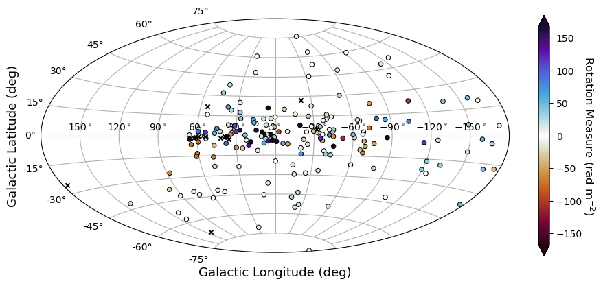
Figure 2: The positions of the MSPs in this sample on an Aitoff projection, with coloured circles indicating sources with measured RMs (including those formally consistent with zero) and black ‘x’ markers indicating sources without measured RMs, as described in the text.

We show in Figure 2 the positions of the MSPs in our sample, coloured by their measured RM (black marks indicate the positions of pulsars without measured RMs). Overall, the RMs for our sample do not indicate strong (average) magnetic fields along the lines of sight, with 90% of values in the range $-$2.8 - 2.3 $\upmu$G (full range $-$6.7 - 5.0 $\upmu$G).

4 Flux Densities and Spectral Indices

Ideally, pulsar flux densities are obtained using an injected and pulsed broadband calibration signal that can be measured against a source of known flux density to derive a flux scale. While attempting to derive a polarisation calibration solution using the MeerKAT L-Band receiver pulsed cal, we found that the degree of polarisation of the cal often exceeds 105%. This is probably due to the strength of the cal being comparable to the system equivalent flux density and driving the system into a non-linear regime. This made this conventional method unsuitable for absolute flux calibration.

An alternative calibration method involves using the radiometer equation and assuming that the rms of the pulsar baseline region is well-defined by the system equivalent flux density plus the galactic sky temperature divided by the antenna gain. In the presence of unrecognised sources of noise due to RFI, this method can underestimate radio fluxes and must be approached with caution. Nevertheless, as shown in Bailes et al. (2020), there are many parts of the MeerKAT L-band (856-1712 MHz) that are almost always devoid of interference, and we found that many of our high DM (DM $\gtrsim 100$ pc cm^-3) sources gave very reliable $S/N$ and hence flux values from epoch to epoch across much of the band. To assess the reliability of this method, we computed the modulation indices of the derived flux densities for the five pulsars with the largest DMs in our sample and found them to be between 7-15%, which means that the reliability of the flux densities from epoch to epoch is probably no worse than this figure.

Absolute flux densities for each observation were thus calculated using the radiometer equation and assuming the Haslam et al. (1981) sky temperatures scale as the observing frequency to the power $-2.55$ (Lawson et al., 1987). To determine mean pulsar flux densities the integrated flux above a baseline is often computed by firstly converting the counts to Jy in a calibration procedure. The mean pulsed flux is then just the integral of the flux above a defined baseline divided by the number of bins. Millisecond pulsars can have profiles that are very complex and this makes baseline estimation difficult if using a simple boxcar, especially if it extends into the wings of the pulse profile. For every MSP, the ideal boxcar width will differ, or even require multiple disjoint sections, so we used an interactive tool to define the baseline through visual inspection for each pulsar from high $S/N$ observations to help determine the rms of the noise in the baseline. Software was written to cross-correlate the template with each profile, and the rms residual of the phase-aligned profiles in the baseline region was evaluated.

There are sections of the MeerKAT band that are rarely affected by RFI (see Bailes et al. 2020), and these were used to determine the flux density in those bands. We found that many of the high-DM MSPs that would be expected to have consistent epoch to epoch flux densities often exhibited dips in their mean spectra where RFI is regularly present in the fourth of the 8 sub-bands. As an example, for PSR J1017$-$7156, the off-pulse rms was roughly 5-21% higher in this band with a mean 10% higher after our attempts at RFI removal with CoastGuard. Scaling the flux densities of all channels by the ratio of their off-pulse rms counts to that of the median off-pulse rms counts led to mean spectra largely free of this dip in channel 4 and was performed on all the data.

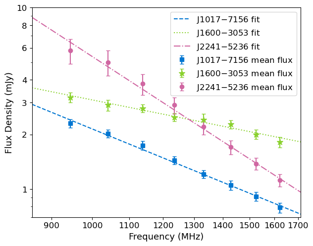
Figure 3: Mean flux density measurements for 3 pulsars, PSRs J1017$-$7156 (blue squares; $N_{\rm obs}=51$), J1600$-$3053 (green stars; $N_{\rm obs}=33$), and J2241$-$5236 (pink circles; $N_{\rm obs}=42$), fit with power law models (blue dashed, green dotted, and pink dash-dotted lines, respectively) to determine $S_{1400}$ and the spectral index, $\alpha$. The power law models for these pulsars are: $S_{1017}=1.09\,{\rm mJy}\times(\nu/1400\,{\rm MHz})^{-2.01}$, $S_{1600}=2.22\,{\rm mJy}\times(\nu/1400\,{\rm MHz})^{-0.99}$, and$S_{2241}=1.83\,{\rm mJy}\times(\nu/1400\,{\rm MHz})^{-3.20}$. The error bars indicate the formal error on the means.

After integrating all of the observations for each pulsar, the vast majority of our pulsars were shown to have a smooth power law variation of mean flux density with frequency as is often seen in the population between 1-1.7 GHz, especially those at high dispersion ($\gtrsim 100$ pc cm^-3) where strong scintillation events across $\sim$100-MHz bands are not seen (Dai et al. 2015; see also Fig. 3, showing PSRs J1017$-$7156, J1600$-$3053, and J2241$-$5236, with DMs of 94.2, 52.3, and 11.4 pc cm^-3, respectively). To derive spectral indices and normalise our flux density measurements to a standard frequency (1400 MHz), we fitted a power-law model, $S=S_{1400}\,(\nu/1400\,\textrm{MHz})^{\alpha}$, to the mean flux density in each of 8 sub-bands across the 775.75 MHz band, and our results are listed in Table 1. In Figure 3, we show an example of the flux density measurements and best-fitting models for 3 pulsars with varying DM values, selected for comparison with the study by Dai et al. (2015) on pulsars in the Parkes Pulsar Timing Array (PPTA) (Kerr et al., 2020).

We refer the reader to Gitika et al. (in prep.) for a thorough analysis of the flux density measurements from these and more recent MeerTime MSP observations, and here we provide a simple comparison of our results with overlapping samples from Dai et al. (2015) and Alam et al. (2021a) to verify the accuracy of our method. Note that the Dai et al. (2015) spectral indices were derived from flux density measurements in 3 bands centred at 732, 1369, and 3100 MHz, and therefore they may be sensitive to, e.g., spectral turn-over, which is possibly seen in their analysis of PSR J1600$-$3053. With this caveat, we find good agreement between our $S_{1400}$ values and spectral indices and those of Dai et al. (2015), with PSR J1744$-$1134 showing the greatest disparities in both $S_{1400}$ and spectral index (although the values are consistent at the 2-$\sigma$ level and this pulsar has a very small DM which makes it prone to large flux density variations). The flux density of this pulsar in the 97-Mhz sub-band centred at 1429 MHz varied from 0.14 to 14 mJy with a mean of 3.7 mJy and a standard deviation of 4.0 mJy. Thus its difference in mean flux density is not that worrying.

Recently, the North American Nanohertz Observatory for Gravitational Waves (NANOGrav) collaboration presented a comprehensive study of flux densities for its sample with which we have significant overlap (Alam et al., 2021a). Of the 15 non-PPTA pulsars for which we have common data, 12 had flux densities within $\sim$30% of our values and those with the largest deviations (differing by roughly a factor of 2 from our values) have low DMs. Alam et al. (2021a) pointed out that the median flux they obtained for PSR J2317+1439 ($0.45^{+0.35}_{-0.19}$ mJy) differed from the catalogue flux density of 4(1) mJy significantly. Our mean value 0.60(6) mJy (median of 0.37 mJy) is much closer to the Alam et al. (2021a) result, and we note that this pulsar scintillates strongly. The pulsar with the most observations (134 with reliable fluxes) was PSR J1909$-$3744. Alam et al. (2021a) measured a median flux density at 1400 MHz of 1.03 mJy, matching our median value precisely, which gives us great confidence in our relative flux density scales. This pulsar experiences extreme scintillation events, and our measured mean flux density was 1.80(9) mJy. Dai et al. (2015) recorded a mean flux density for PSR J1909$-$3744 of 2.5(2) mJy at 1400 MHz. Note also that different observing strategies can lead to biases in observed flux density distributions. MeerKAT observations use a queue system with minimal intervention (and NANOGrav observations are run with minimal intervention), while observations for the PPTA are done manually, and observers are encouraged to switch sources when the source $S/N$ is low and to repeat observations when the $S/N$ is high. This leads to better uncertainties on the times of arrival but biases the flux density distributions to higher values, which is consistent with our results.

Overall, we find a mean spectral index of $-1.92(6)$, with a standard deviation of 0.6, for our sample of 189 pulsars, and we show the full distribution of spectral indices in Figure 4. This mean is consistent at the 2-$\sigma$ level with that found by Dai et al. (2015), who found a value of $-1.81(1)$, as well as previous results for MSP studies (Toscano et al., 1998; Kramer et al., 1999) and studies of normal pulsars (Jankowski et al., 2018). The typical uncertainties on the spectral indices for pulsars with $>10$ observations are $\sim 0.1$, with 95% of the uncertainties $<0.4$. These results could be improved in future using the MeerKAT UHF and S-band receivers to increase the frequency coverage.

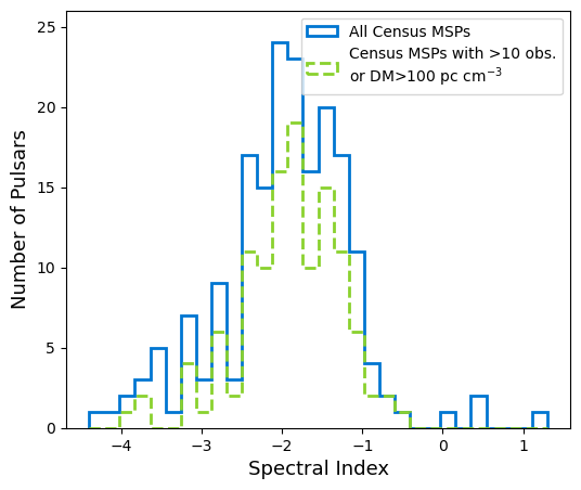
Figure 4: Histogram of spectral indices. In green, we show the spectral indices for pulsars with DM $>\,100$ pc cm^-3 (and therefore low scintillation) and those with $>\,10$ observations to reduce the impact of scintillation on the measurements. We show the remaining spectral indices in our sample in the blue histogram.

5 Timing Results

For all pulsars in this study, we list basic parameters in Table 1, and provide our measured median ToA uncertainties. The templates used for our standard timing procedure are produced from summed, temporally-integrated observations with 232 frequency channels across the 775.75-MHz band. From these high-$S/N$ observations, we then derive pulse “portraits” using the PulsePortraiture software (Pennucci, 2019) and produce noise-free templates with 8 sub-bands for timing. We use the “Fourier Domain with Markov chain Monte Carlo” (FDM) fitting algorithm from pat in psrchive to produce ToAs from archives partially-integrated to 256-second sub-integrations and 8 sub-bands across the 775.75-MHz band ($\sim 97$-MHz sub-bands). We compute “typical” ToA uncertainties per pulsar by first normalising the measured uncertainties to the nominal minimum observing time, 256 s, then calculating the error on the weighted mean ToA for each sub-integration as

$$\frac{1}{\sigma_{\textrm{sub}}^{2}}=\sum_{i}\frac{1}{\sigma_{\textrm{sub,}i}^{2}},$$ (4)

where i represents the frequency channels, and finally returning the median of the resulting $\sigma_{\textrm{sub}}$ values as the typical ToA uncertainty. We note that this method approximates the ToA uncertainty achievable by proper wide-band timing using a 2-dimensional template (i.e., returning a single ToA per sub-integration). We summarise the resulting median ToA uncertainties in Figure 5, showing the cumulative histogram of the median uncertainties. Note that the median ToA uncertainties should not be confused with the ultimate fitted rms residuals, as they do not factor in pulse jitter nor the deleterious effects of red noise.

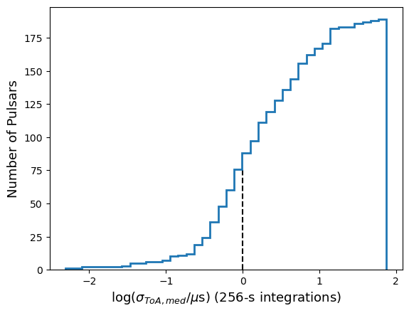
Figure 5: Cumulative histogram of median ToA uncertainties from 97-MHz, 256-second sub-integrations, scaled to the full 775.75 MHz, on a logarithmic scale. From these data, 77 pulsars have sub-microsecond (median) timing precision in less than 256 seconds.

5.1 Timing Forecast

In assembling a large dataset of MSP data across a minimum timespan of six months, we are able to determine the timing potential for each source and inform future studies. The potential for MeerTime to contribute to global efforts to detect GWs with the IPTA can be estimated from these data. As mentioned in section 2, we continue to regularly observe pulsars that have low ToA uncertainties, $\sigma_{\tau}<1\,\upmu$s, calculated using frequency-scrunched templates and observations with integration times, $256<T_{\textrm{obs}}<2000$ s.

To compare the sensitivity of PTA observations with MeerKAT to other current programmes, and its potential impact on global efforts, we consider the detection of a GW background (assuming a strain spectrum of $h_{c}(f)=1.9\times 10^{-15}(f/1\,{\rm yr})^{-2/3}$; e.g., Siemens et al. 2013) through correlations between pulsars in the array (Hellings & Downs, 1983). The background is chosen to be the amplitude of the apparent common red noise found in analysis of the NANOGrav 12.5-year data release (Alam et al., 2021b). We can approximate the sensitivity of a given PTA to both the auto-correlated signal (the “pulsar term”) and the cross-correlated signal (the “Earth term”), following Siemens et al. (2013). They construct matched detection statistics in the Fourier domain (see their Equation 17) and calculate how the signal to noise ratio of the detection statistic depends on the noise properties of the array.

The expected signal-to-noise ratio in the autocorrelations is

$$\rho_{ACF}^{2}=\sum_{p=1}^{N_{p}}\sum_{k=1}^{N_{f}}\frac{P_{g}^{2}(f_{k})}{P_{p}^{2}(f_{k})},$$ (5)

where $P_{g}(f_{k})$ is the power spectral density of the GWB in frequency channel $f_{k}$, where $k=1,N_{f}$ is a Fourier series starting $1/T_{eff}$ at the reciprocal of the common effective observing $T_{\rm eff}$. $P_{p}(f_{k})=P_{g}(f_{k})+P_{p,r}(f_{k})+P_{p,w}$ is the total power (the sum of the GWB and the red noise ($P_{p,r}$) and the white noise ($P_{w,r}$) in the same channel for pulsar $p$.

The expected signal-to-noise ratio in the cross correlations is found as the S/N of a matched filter with the Hellings-Downs correlation function

$$\rho^{2}=\sum_{i=1}^{N_{p}-1}\sum_{j=i+1}^{N_{p}}\chi^{2}_{ij}\sum_{k=1}^{N_{f}}\frac{P^{2}_{g}(f_{k})}{P_{p_{i}}(f_{k})P_{p_{j}}(f_{k})},$$ (6)

where $\chi_{ij}$ are the angular correlation coefficients Hellings & Downs (1983)

$$\begin{split}\chi_{ij}=\frac{3}{4}\left(1-\cos(\theta_{ij})\right)&\log\left(1-\cos(\theta_{ij})\right)\\ &-\frac{1}{8}\left(1-\cos(\theta_{ij})\right)+\frac{1}{2}\end{split}$$ (7)

We use the published source lists, median pulsar timing precisions, timespans, cadences, and observational parameters from the European Pulsar Timing Array (EPTA; Desvignes et al., 2016), NANOGrav (Alam et al., 2021b), and the PPTA (Kerr et al., 2020) to form a representative sample of the IPTA. For sources in multiple PTAs, the data set with the longest time span is used. We show how the $S/N$ for this background increases with time in Figure 6.

For the NANOGrav sensitivity curves, we have assumed that the Arecibo timing programme ceased in August 2020 and that the pulsars are not observed elsewhere, which demonstrates the importance of Arecibo to international pulsar timing efforts. The modelling includes red noise in the sensitivity estimates, for pulsars where red noise has previously been detected (Arzoumanian et al., 2020; Goncharov et al., 2021). Undetected red noise is likely to be present in some of the pulsars timed by MeerKAT, which will affect our sensitivity estimates.

These calculations imply that the MPTA will be comparable in sensitivity to the PPTA by 2023, NANOGrav by 2024, and the EPTA by $\approx 2025$. In less than four years, the MPTA will be contributing to the IPTA effort. As the MeerKAT timing array programme has observed a large number of pulsars from its start, the sensitivity to the cross correlated signal (dashed lines) is always comparable to the auto-correlated signal, similar to the EPTA with its 42 pulsars. In contrast, the PPTA project includes only 26 pulsars, and NANOGrav started out with a smaller number of pulsars before gradually increasing in size starting in 2009, and, in the most recent data release (12.5-yr), they listed 47 pulsars (Alam et al., 2021b). The MPTA could be expanded in the future with timing of additional pulsars in other bands or timing of MSPs discovered by MeerKAT and other facilities. Future work by Middleton et al. (2022, in prep.) will examine the sensitivity of the MPTA and potential improvements.

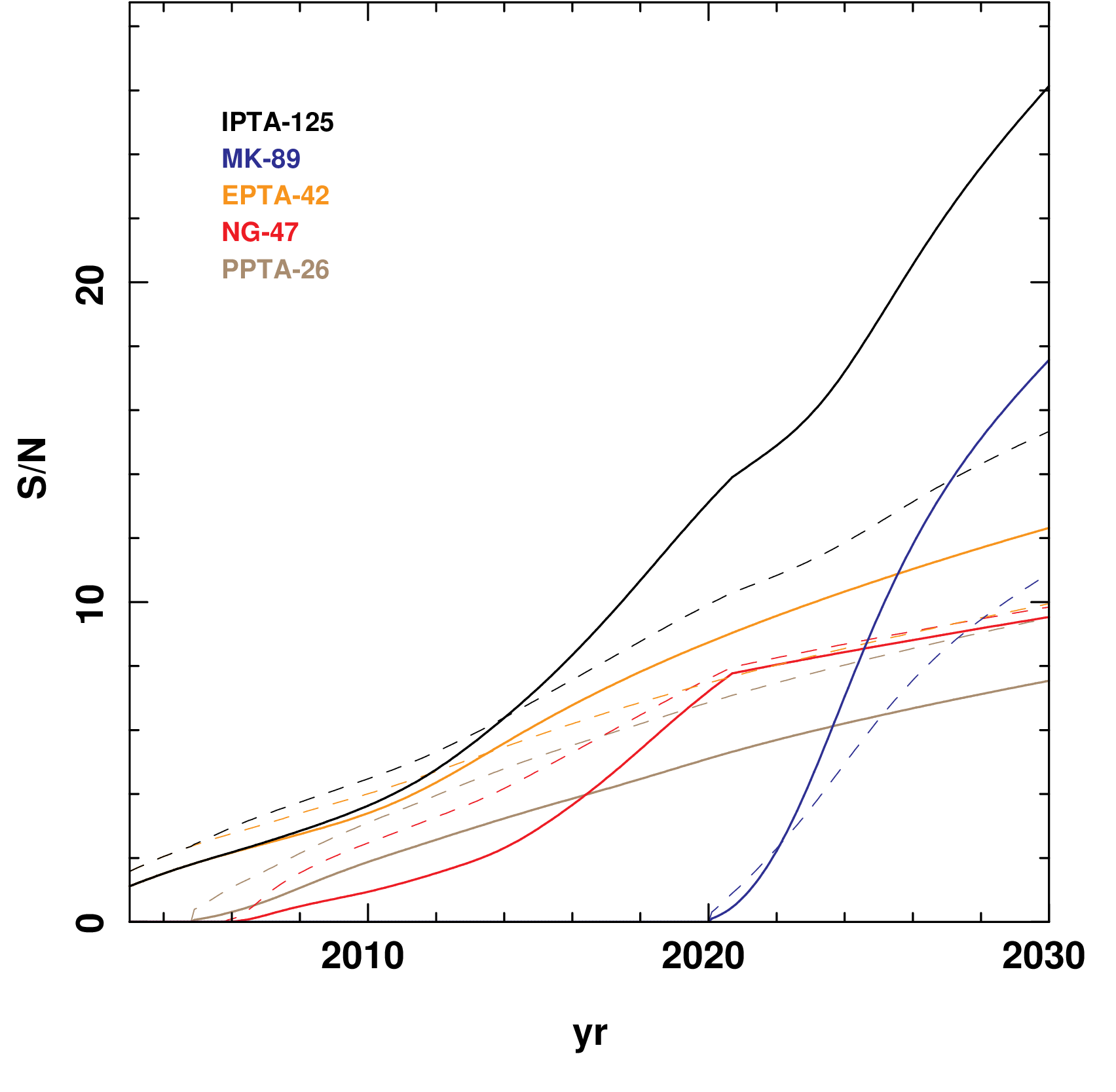
Figure 6: Comparison of PTA sensitivity to the cross-correlated component of the GW background (solid lines) and the uncorrelated signal (dashed lines), using the current MeerTime timing programme with 89 pulsars (blue lines), the European Pulsar Timing Array (EPTA) programme with 42 pulsars (orange lines), the NANOGrav programme with 47 sources (red lines), the PPTA with 26 (brown lines), or the IPTA as the union of the four (black lines).

6 Summary

In this work, we demonstrated the outstanding potential of MeerKAT for precision pulsar timing of MSPs with this initial census, analysing polarization properties, flux densities and spectral indices, and timing precision. We presented a dataset of nearly 4000 observations of 189 pulsars, spanning 24 months, including polarization-calibrated profiles and high-precision ToAs. Our timing simulations offer simple predictions of future results, and we predict that the MPTA will be a major contributor to global PTA efforts within the next 5 years. More work is forthcoming, including the first MPTA data release with full timing and noise analyses (Miles et al., 2022, in prep.), an analysis of flux density measurements for MeerTime MSPs (Gitika et al., in prep.), and a study of the sensitivity of the MPTA and potential for improvements (Middleton et al., 2022, in prep.).

Data Availability

We have made available all 189 polarization profiles, as shown in Figures 7–27, in PSRFITS format with full phase resolution (1024 bins), 4 polarization channels, and 8 frequency channels across the 775.75-MHz band, as well as the table containing the analysis results. The table, in csv format with 189 rows, contains mean flux densities (and standard deviations) in 8 frequency bands per pulsar, spectral indices and fit $S_{1400}$ values with uncertainties, median timing uncertainties as described in section 5, polarization fractions and rotation measures, dispersion measures and reference epochs, and basic pulsar properties (rotation properties and positions) for easy reference. The dataset will be made available prior to publication of this manuscript, under the DOI 10.5281/zenodo.5347875.

Appendix A Polarization Profiles

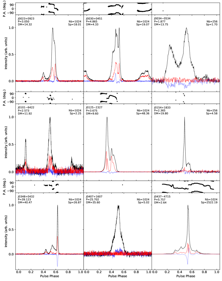
Figure 7: Polarization profiles for MSPs from the MeerTime Census project, fully integrated from the 775.75-MHz band centred at 1284 MHz, with polarization position angles in the upper panels (not corrected to infinite frequency). The black solid line indicates the total intensity, the red dashed line shows the linearly polarized emission, and the blue dotted line shows the circularly polarized emission. All profiles show the phase range ($-$0.05, 1.05), and P.A.s are plotted over the range ($-$135, 135) degrees. The period and DM of each source is listed in the upper left corner, in units of ms and pc cm^-3, respectively. In the upper right corner, we indicate the number of phase bins used (256 for $P<15$ ms and low $S/N$) and the normalisation factor (peak flux density at 1284 MHz in mJy).

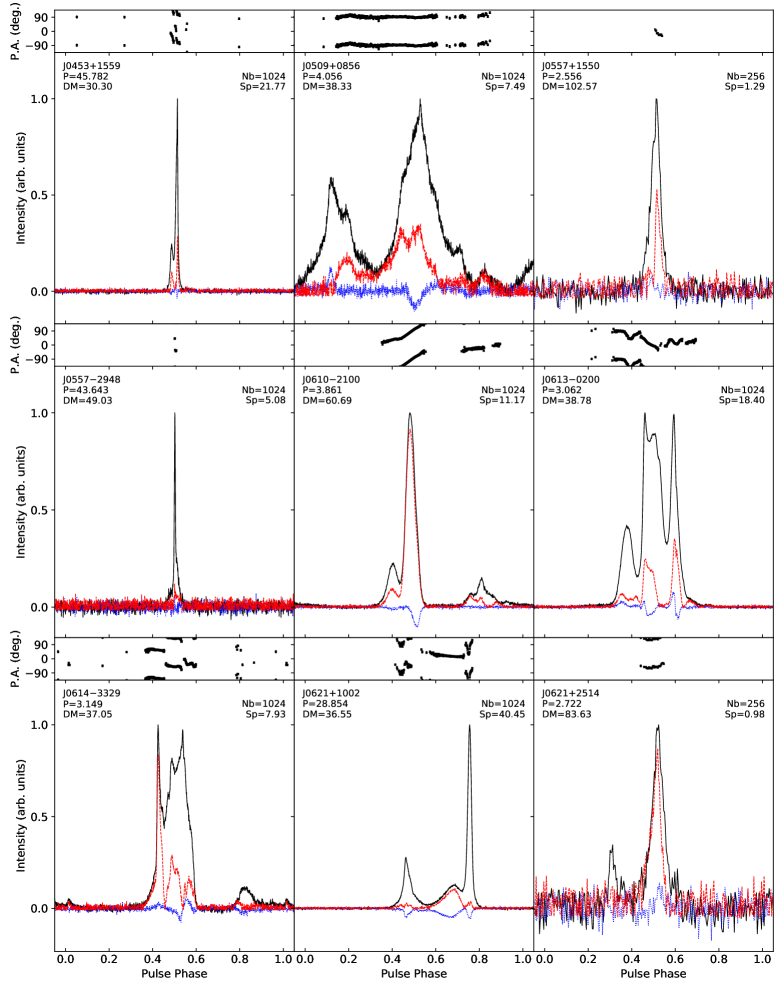
Figure 8: Polarization profiles for MSPs from the MeerTime Census project, as Fig. 7.

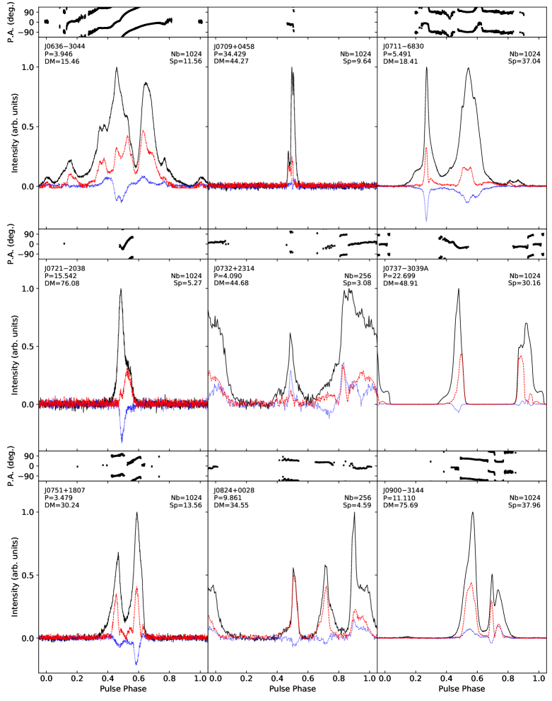
Figure 9: Polarization profiles for MSPs from the MeerTime Census project, as Fig. 7.

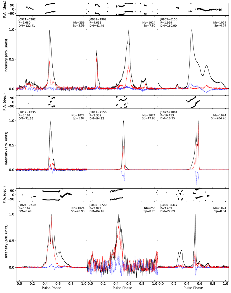
Figure 10: Polarization profiles for MSPs from the MeerTime Census project, as Fig. 7.

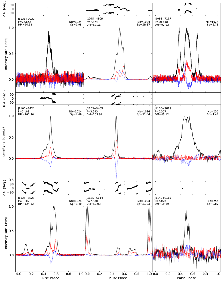
Figure 11: Polarization profiles for MSPs from the MeerTime Census project, as Fig. 7.

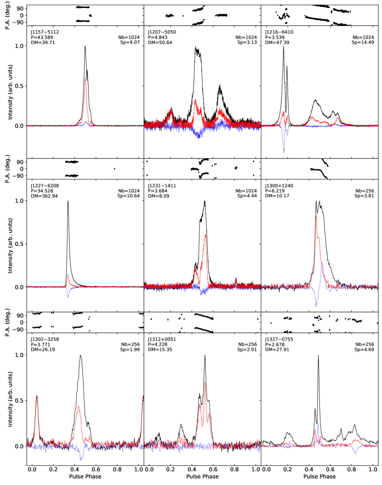
Figure 12: Polarization profiles for MSPs from the MeerTime Census project, as Fig. 7.

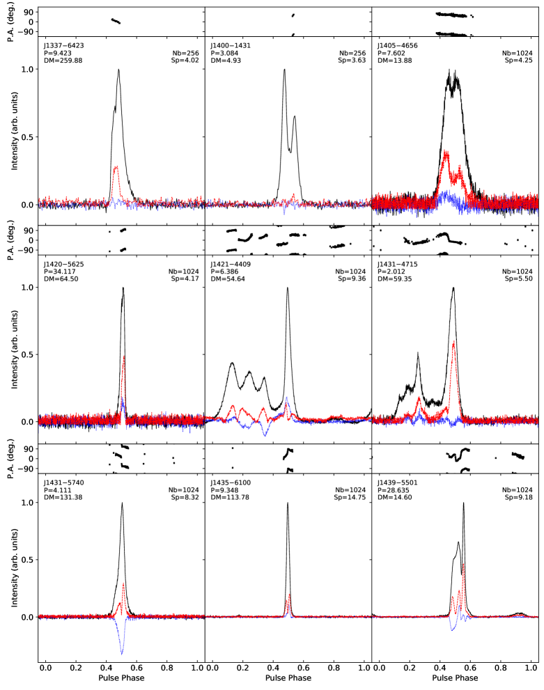
Figure 13: Polarization profiles for MSPs from the MeerTime Census project, as Fig. 7.

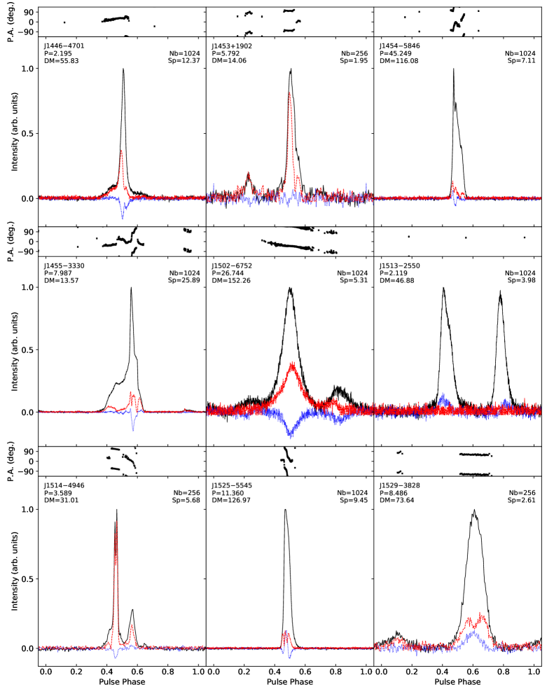
Figure 14: Polarization profiles for MSPs from the MeerTime Census project, as Fig. 7.

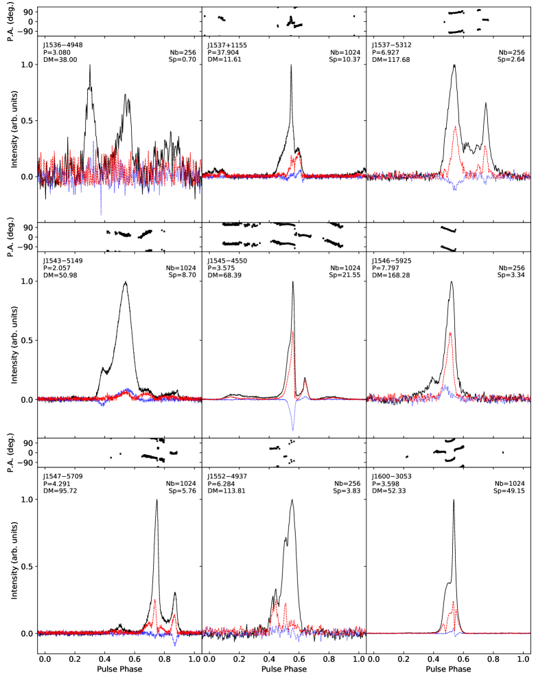
Figure 15: Polarization profiles for MSPs from the MeerTime Census project, as Fig. 7.

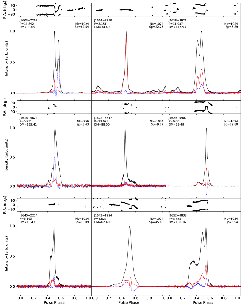
Figure 16: Polarization profiles for MSPs from the MeerTime Census project, as Fig. 7.

Figure 17: Polarization profiles for MSPs from the MeerTime Census project, as Fig. 7.

Figure 18: Polarization profiles for MSPs from the MeerTime Census project, as Fig. 7.

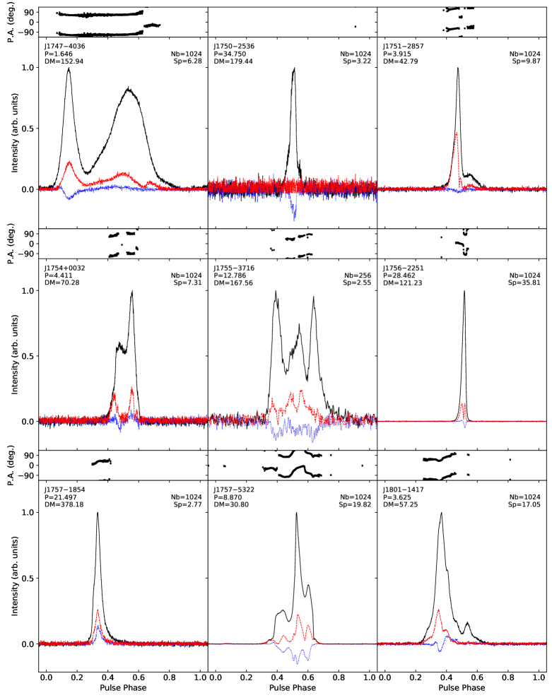
Figure 19: Polarization profiles for MSPs from the MeerTime Census project, as Fig. 7.

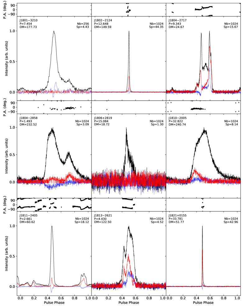
Figure 20: Polarization profiles for MSPs from the MeerTime Census project, as Fig. 7.

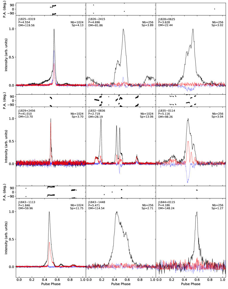
Figure 21: Polarization profiles for MSPs from the MeerTime Census project, as Fig. 7.

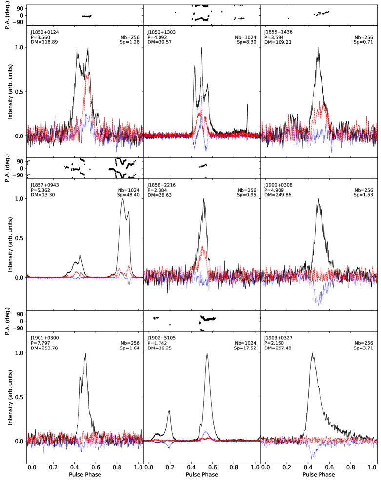
Figure 22: Polarization profiles for MSPs from the MeerTime Census project, as Fig. 7.

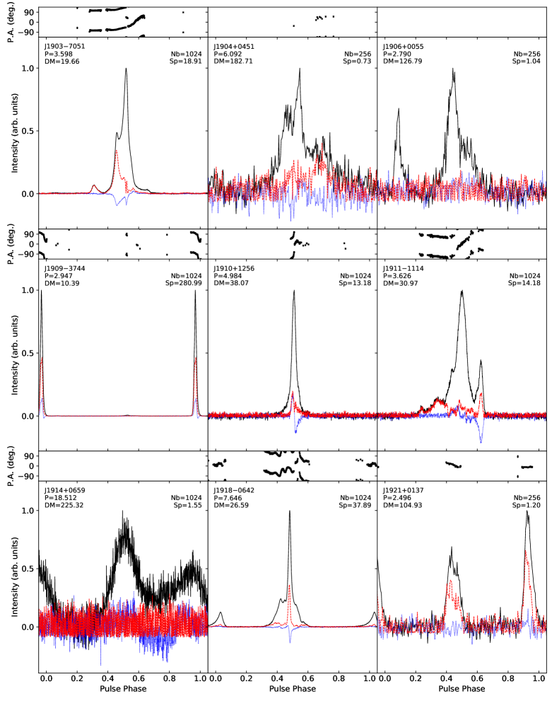
Figure 23: Polarization profiles for MSPs from the MeerTime Census project, as Fig. 7.

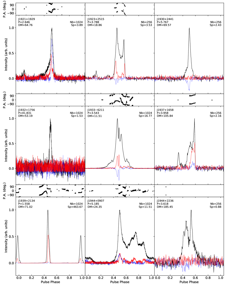
Figure 24: Polarization profiles for MSPs from the MeerTime Census project, as Fig. 7.

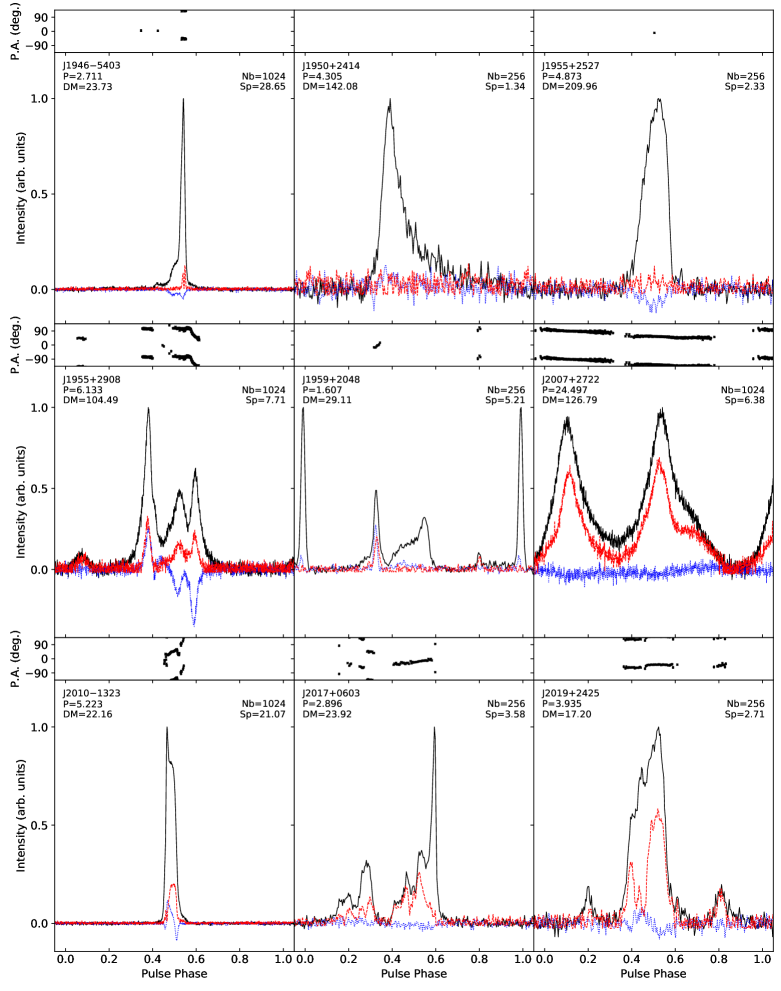
Figure 25: Polarization profiles for MSPs from the MeerTime Census project, as Fig. 7.

Figure 26: Polarization profiles for MSPs from the MeerTime Census project, as Fig. 7.

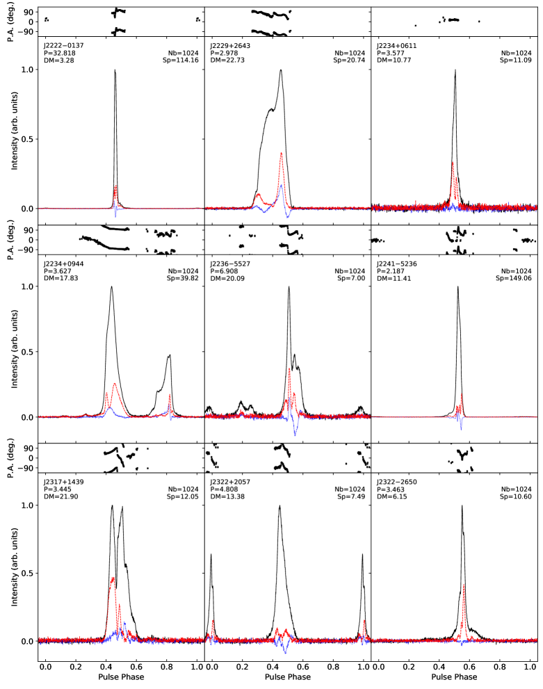
Figure 27: Polarization profiles for MSPs from the MeerTime Census project, as Fig. 7.

References

- \definecolordarkbluergb0,0,0.597656
- Alam et al. (2021a) Alam M. F., et al., 2021a, \textcolordarkblueApJS, 252, 4
- Alam et al. (2021b) Alam M. F., et al., 2021b, \textcolordarkblueApJS, 252, 5
- Alpar et al. (1982) Alpar M. A., Cheng A. F., Ruderman M. A., Shaham J., 1982, \textcolordarkblueNature, 300, 728
- Arzoumanian et al. (2020) Arzoumanian Z., et al., 2020, \textcolordarkblueApJ, 905, L34
- Backer et al. (1982) Backer D. C., Kulkarni S. R., Heiles C., Davis M. M., Goss W. M., 1982, \textcolordarkblueNature, 300, 615
- Bailes (1989) Bailes M., 1989, \textcolordarkblueApJ, 342, 917
- Bailes et al. (1994) Bailes M., et al., 1994, \textcolordarkblueApJ, 425, L41
- Bailes et al. (1997) Bailes M., et al., 1997, \textcolordarkblueApJ, 481, 386
- Bailes et al. (2011) Bailes M., et al., 2011, \textcolordarkblueScience, 333, 1717
- Bailes et al. (2020) Bailes M., et al., 2020, \textcolordarkbluePASA, 37, e028
- Barr et al. (2013) Barr E. D., et al., 2013, \textcolordarkblueMNRAS, 429, 1633
- Bates et al. (2015) Bates S. D., et al., 2015, \textcolordarkblueMNRAS, 446, 4019
- Bhattacharya & van den Heuvel (1991) Bhattacharya D., van den Heuvel E. P. J., 1991, \textcolordarkbluePhys. Rep., 203, 1
- Bhattacharyya et al. (2016) Bhattacharyya B., et al., 2016, \textcolordarkblueApJ, 817, 130
- Bisnovatyi-Kogan & Komberg (1974) Bisnovatyi-Kogan G. S., Komberg B. V., 1974, Soviet Ast., 18, 217
- Boriakoff et al. (1983) Boriakoff V., Buccheri R., Fauci F., 1983, \textcolordarkblueNature, 304, 417
- Boyles et al. (2013) Boyles J., et al., 2013, \textcolordarkblueApJ, 763, 80
- Burgay et al. (2003) Burgay M., et al., 2003, \textcolordarkblueNature, 426, 531
- Burgay et al. (2006) Burgay M., et al., 2006, \textcolordarkblueMNRAS, 368, 283
- Burgay et al. (2013a) Burgay M., et al., 2013a, \textcolordarkblueMNRAS, 429, 579
- Burgay et al. (2013b) Burgay M., et al., 2013b, \textcolordarkblueMNRAS, 433, 259
- Burgay et al. (2019) Burgay M., et al., 2019, \textcolordarkblueMNRAS, 484, 5791
- Cameron et al. (2018) Cameron A. D., et al., 2018, \textcolordarkblueMNRAS, 475, L57
- Cameron et al. (2020) Cameron A. D., et al., 2020, \textcolordarkblueMNRAS, 493, 1063
- Camilo (1995) Camilo F., 1995, PhD thesis, PRINCETON UNIVERSITY.
- Camilo et al. (1993) Camilo F., Nice D. J., Taylor J. H., 1993, \textcolordarkblueApJ, 412, L37
- Camilo et al. (1996) Camilo F., Nice D. J., Shrauner J. A., Taylor J. H., 1996, \textcolordarkblueApJ, 469, 819
- Camilo et al. (2001) Camilo F., et al., 2001, \textcolordarkblueApJ, 548, L187
- Camilo et al. (2015) Camilo F., et al., 2015, \textcolordarkblueApJ, 810, 85
- Champion et al. (2004) Champion D. J., Lorimer D. R., McLaughlin M. A., Cordes J. M., Arzoumanian Z., Weisberg J. M., Taylor J. H., 2004, \textcolordarkblueMNRAS, 350, L61
- Champion et al. (2005) Champion D. J., et al., 2005, \textcolordarkblueMNRAS, 363, 929
- Champion et al. (2008) Champion D. J., et al., 2008, \textcolordarkblueScience, 320, 1309
- Chen et al. (2021) Chen S., et al., 2021, \textcolordarkblueMNRAS, 508, 4970
- Clark et al. (2018) Clark C. J., et al., 2018, \textcolordarkblueScience Advances, 4, eaao7228
- Cognard et al. (2011) Cognard I., et al., 2011, \textcolordarkblueApJ, 732, 47
- Cordes et al. (2006) Cordes J. M., et al., 2006, \textcolordarkblueApJ, 637, 446
- Crawford et al. (2006) Crawford F., Roberts M. S. E., Hessels J. W. T., Ransom S. M., Livingstone M., Tam C. R., Kaspi V. M., 2006, \textcolordarkblueApJ, 652, 1499
- Crawford et al. (2012) Crawford F., et al., 2012, \textcolordarkblueApJ, 757, 90
- Dai et al. (2015) Dai S., et al., 2015, \textcolordarkblueMNRAS, 449, 3223
- Demorest et al. (2010) Demorest P. B., Pennucci T., Ransom S. M., Roberts M. S. E., Hessels J. W. T., 2010, \textcolordarkblueNature, 467, 1081
- Deneva et al. (2012) Deneva J. S., et al., 2012, \textcolordarkblueApJ, 757, 89
- Deneva et al. (2013) Deneva J. S., Stovall K., McLaughlin M. A., Bates S. D., Freire P. C. C., Martinez J. G., Jenet F., Bagchi M., 2013, \textcolordarkblueApJ, 775, 51
- Desvignes et al. (2016) Desvignes G., et al., 2016, \textcolordarkblueMNRAS, 458, 3341
- Eatough et al. (2009) Eatough R. P., Keane E. F., Lyne A. G., 2009, \textcolordarkblueMNRAS, 395, 410
- Edwards & Bailes (2001a) Edwards R. T., Bailes M., 2001a, \textcolordarkblueApJ, 547, L37
- Edwards & Bailes (2001b) Edwards R. T., Bailes M., 2001b, \textcolordarkblueApJ, 553, 801
- Everett & Weisberg (2001) Everett J. E., Weisberg J. M., 2001, \textcolordarkblueApJ, 553, 341
- Faulkner et al. (2004) Faulkner A. J., et al., 2004, \textcolordarkblueMNRAS, 355, 147
- Foster et al. (1993) Foster R. S., Wolszczan A., Camilo F., 1993, \textcolordarkblueApJ, 410, L91
- Foster et al. (1995) Foster R. S., Cadwell B. J., Wolszczan A., Anderson S. B., 1995, \textcolordarkblueApJ, 454, 826
- Fruchter et al. (1988) Fruchter A. S., Stinebring D. R., Taylor J. H., 1988, \textcolordarkblueNature, 333, 237
- Geyer et al. (2021) Geyer M., et al., 2021, \textcolordarkblueMNRAS, 505, 4468
- Goncharov et al. (2021) Goncharov B., et al., 2021, \textcolordarkblueApJ, 917, L19
- Han et al. (2018) Han J. L., Manchester R. N., van Straten W., Demorest P., 2018, \textcolordarkblueApJS, 234, 11
- Haslam et al. (1981) Haslam C. G. T., Klein U., Salter C. J., Stoffel H., Wilson W. E., Cleary M. N., Cooke D. J., Thomasson P., 1981, A&A, 100, 209
- Hellings & Downs (1983) Hellings R. W., Downs G. S., 1983, \textcolordarkblueApJ, 265, L39
- Hessels et al. (2011) Hessels J. W. T., et al., 2011, in Burgay M., D’Amico N., Esposito P., Pellizzoni A., Possenti A., eds, American Institute of Physics Conference Series Vol. 1357, American Institute of Physics Conference Series. pp 40–43 (arXiv:1101.1742), \textcolordarkbluedoi:10.1063/1.3615072
- Hobbs et al. (2004) Hobbs G., et al., 2004, \textcolordarkblueMNRAS, 352, 1439
- Hotan et al. (2004) Hotan A. W., van Straten W., Manchester R. N., 2004, \textcolordarkbluePASA, 21, 302
- Hulse & Taylor (1975) Hulse R. A., Taylor J. H., 1975, \textcolordarkblueApJ, 195, L51
- Hunter (2007) Hunter J. D., 2007, \textcolordarkblueComputing In Science & Engineering, 9, 90
- Jacoby (2005) Jacoby B. A., 2005, PhD thesis, California Institute of Technology, California, USA
- Jacoby et al. (2003) Jacoby B. A., Bailes M., van Kerkwijk M. H., Ord S., Hotan A., Kulkarni S. R., Anderson S. B., 2003, \textcolordarkblueApJ, 599, L99
- Jacoby et al. (2007) Jacoby B. A., Bailes M., Ord S. M., Knight H. S., Hotan A. W., 2007, \textcolordarkblueApJ, 656, 408
- Jankowski et al. (2018) Jankowski F., van Straten W., Keane E. F., Bailes M., Barr E. D., Johnston S., Kerr M., 2018, \textcolordarkblueMNRAS, 473, 4436
- Johnston & Bailes (1991) Johnston S., Bailes M., 1991, \textcolordarkblueMNRAS, 252, 277
- Johnston et al. (1993) Johnston S., et al., 1993, \textcolordarkblueNature, 361, 613
- Johnston et al. (2020) Johnston S., et al., 2020, \textcolordarkblueMNRAS, 493, 3608
- Jonas & MeerKAT Team (2016) Jonas J., MeerKAT Team 2016, in MeerKAT Science: On the Pathway to the SKA. p. 1
- Kawash et al. (2018) Kawash A. M., et al., 2018, \textcolordarkblueApJ, 857, 131
- Keane et al. (2018) Keane E. F., et al., 2018, \textcolordarkblueMNRAS, 473, 116
- Keith et al. (2010) Keith M. J., et al., 2010, \textcolordarkblueMNRAS, 409, 619
- Keith et al. (2011) Keith M. J., et al., 2011, \textcolordarkblueMNRAS, 414, 1292
- Keith et al. (2012) Keith M. J., et al., 2012, \textcolordarkblueMNRAS, 419, 1752
- Kerr et al. (2012) Kerr M., et al., 2012, \textcolordarkblueApJ, 748, L2
- Kerr et al. (2020) Kerr M., et al., 2020, arXiv e-prints, p. arXiv:2003.09780
- Knispel et al. (2010) Knispel B., et al., 2010, \textcolordarkblueScience, 329, 1305
- Knispel et al. (2013) Knispel B., et al., 2013, \textcolordarkblueApJ, 774, 93
- Knispel et al. (2015) Knispel B., et al., 2015, \textcolordarkblueApJ, 806, 140
- Kramer & Xilouris (2000) Kramer M., Xilouris K. M., 2000, in Kramer M., Wex N., Wielebinski R., eds, Astronomical Society of the Pacific Conference Series Vol. 202, IAU Colloq. 177: Pulsar Astronomy - 2000 and Beyond. p. 229 (arXiv:astro-ph/0002115)
- Kramer et al. (1998) Kramer M., Xilouris K. M., Lorimer D. R., Doroshenko O., Jessner A., Wielebinski R., Wolszczan A., Camilo F., 1998, \textcolordarkblueApJ, 501, 270
- Kramer et al. (1999) Kramer M., Lange C., Lorimer D. R., Backer D. C., Xilouris K. M., Jessner A., Wielebinski R., 1999, \textcolordarkblueApJ, 526, 957
- Kramer et al. (2021) Kramer M., et al., 2021, \textcolordarkblueMNRAS, 504, 2094
- Laffon et al. (2015) Laffon H., Smith D. A., Guillemot L., 2015, arXiv e-prints, p. arXiv:1502.03251
- Lawson et al. (1987) Lawson K. D., Mayer C. J., Osborne J. L., Parkinson M. L., 1987, \textcolordarkblueMNRAS, 225, 307
- Lazarus et al. (2015) Lazarus P., et al., 2015, \textcolordarkblueApJ, 812, 81
- Lazarus et al. (2020) Lazarus P., Karuppusamy R., Graikou E., Caballero R. N., Champion D. J., Lee K. J., Verbiest J. P. W., Kramer M., 2020, CoastGuard: Automated timing data reduction pipeline (ascl:2003.008)
- Lee et al. (2012) Lee K. J., Guillemot L., Yue Y. L., Kramer M., Champion D. J., 2012, \textcolordarkblueMNRAS, 424, 2832
- Levin et al. (2013) Levin L., et al., 2013, \textcolordarkblueMNRAS, 434, 1387
- Levin et al. (2018) Levin L., et al., 2018, in Weltevrede P., Perera B. B. P., Preston L. L., Sanidas S., eds, Vol. 337, Pulsar Astrophysics the Next Fifty Years. pp 171–174 (arXiv:1712.01008), \textcolordarkbluedoi:10.1017/S1743921317009528
- Lommen et al. (2000) Lommen A. N., Zepka A., Backer D. C., McLaughlin M., Cordes J. M., Arzoumanian Z., Xilouris K., 2000, \textcolordarkblueApJ, 545, 1007
- Lorimer et al. (1995) Lorimer D. R., et al., 1995, \textcolordarkblueApJ, 439, 933
- Lorimer et al. (1996) Lorimer D. R., Lyne A. G., Bailes M., Manchester R. N., D’Amico N., Stappers B. W., Johnston S., Camilo F., 1996, \textcolordarkblueMNRAS, 283, 1383
- Lorimer et al. (2005) Lorimer D. R., et al., 2005, \textcolordarkblueMNRAS, 359, 1524
- Lorimer et al. (2007) Lorimer D. R., McLaughlin M. A., Champion D. J., Stairs I. H., 2007, \textcolordarkblueMNRAS, 379, 282
- Lundgren et al. (1995) Lundgren S. C., Zepka A. F., Cordes J. M., 1995, \textcolordarkblueApJ, 453, 419
- Lynch et al. (2013) Lynch R. S., et al., 2013, \textcolordarkblueApJ, 763, 81
- Manchester et al. (2001) Manchester R. N., et al., 2001, \textcolordarkblueMNRAS, 328, 17
- Manchester et al. (2005) Manchester R. N., Hobbs G. B., Teoh A., Hobbs M., 2005, \textcolordarkblueAJ, 129, 1993
- Manchester et al. (2013) Manchester R. N., et al., 2013, \textcolordarkbluePASA, 30, e017
- Martinez et al. (2019) Martinez J. G., et al., 2019, \textcolordarkblueApJ, 881, 166
- Matthews et al. (2016) Matthews A. M., et al., 2016, \textcolordarkblueApJ, 818, 92
- McEwen et al. (2020) McEwen A. E., et al., 2020, \textcolordarkblueApJ, 892, 76
- Mickaliger et al. (2012) Mickaliger M. B., et al., 2012, \textcolordarkblueApJ, 759, 127
- Morello et al. (2019) Morello V., et al., 2019, \textcolordarkblueMNRAS, 483, 3673
- Naghizadeh-Khouei & Clarke (1993) Naghizadeh-Khouei J., Clarke D., 1993, A&A, 274, 968
- Navarro et al. (1995) Navarro J., de Bruyn A. G., Frail D. A., Kulkarni S. R., Lyne A. G., 1995, \textcolordarkblueApJ, 455, L55
- Ng et al. (2014) Ng C., et al., 2014, \textcolordarkblueMNRAS, 439, 1865
- Ng et al. (2015) Ng C., et al., 2015, \textcolordarkblueMNRAS, 450, 2922
- Nice et al. (1993) Nice D. J., Taylor J. H., Fruchter A. S., 1993, \textcolordarkblueApJ, 402, L49
- Noll (2010) Noll C. E., 2010, \textcolordarkblueAdvances in Space Research, 45, 1421
- Özel & Freire (2016) Özel F., Freire P., 2016, \textcolordarkblueARA&A, 54, 401
- Parent et al. (2019) Parent E., et al., 2019, \textcolordarkblueApJ, 886, 148
- Parthasarathy et al. (2021) Parthasarathy A., et al., 2021, \textcolordarkblueMNRAS, 502, 407
- Pennucci (2019) Pennucci T. T., 2019, \textcolordarkblueApJ, 871, 34
- Perera et al. (2019) Perera B. B. P., et al., 2019, \textcolordarkblueMNRAS, 490, 4666
- Phinney (1992) Phinney E. S., 1992, \textcolordarkbluePhilosophical Transactions of the Royal Society of London Series A, 341, 39
- Pitkin (2018) Pitkin M., 2018, \textcolordarkblueJournal of Open Source Software, 3, 538
- Price-Whelan et al. (2018) Price-Whelan A. M., et al., 2018, \textcolordarkblueAJ, 156, 123
- Radhakrishnan & Srinivasan (1982) Radhakrishnan V., Srinivasan G., 1982, Current Science, 51, 1096
- Rankin et al. (2017) Rankin J. M., et al., 2017, \textcolordarkblueApJ, 845, 23
- Ransom et al. (2011) Ransom S. M., et al., 2011, \textcolordarkblueApJ, 727, L16
- Ray et al. (1996) Ray P. S., Thorsett S. E., Jenet F. A., van Kerkwijk M. H., Kulkarni S. R., Prince T. A., Sand hu J. S., Nice D. J., 1996, \textcolordarkblueApJ, 470, 1103
- Ray et al. (2012) Ray P. S., et al., 2012, arXiv e-prints, p. arXiv:1205.3089
- Ridolfi et al. (2021) Ridolfi A., et al., 2021, \textcolordarkblueMNRAS, 504, 1407
- Rosen et al. (2013) Rosen R., et al., 2013, \textcolordarkblueApJ, 768, 85
- Roy & Bhattacharyya (2013) Roy J., Bhattacharyya B., 2013, \textcolordarkblueApJ, 765, L45
- Sanidas et al. (2019) Sanidas S., et al., 2019, \textcolordarkblueA&A, 626, A104
- Sanpa-arsa (2016) Sanpa-arsa S., 2016, PhD thesis, University of Virginia, \textcolordarkbluedoi:10.18130/V36K7P
- Scholz et al. (2015) Scholz P., et al., 2015, \textcolordarkblueApJ, 800, 123
- Segelstein et al. (1986) Segelstein D. J., Rawley L. A., Stinebring D. R., Fruchter A. S., Taylor J. H., 1986, \textcolordarkblueNature, 322, 714
- Serylak et al. (2021) Serylak M., et al., 2021, \textcolordarkblueMNRAS, 505, 4483
- Shannon et al. (2013) Shannon R. M., et al., 2013, \textcolordarkblueScience, 342, 334
- Siemens et al. (2013) Siemens X., Ellis J., Jenet F., Romano J. D., 2013, \textcolordarkblueClassical and Quantum Gravity, 30, 224015
- Sobey et al. (2019) Sobey C., et al., 2019, \textcolordarkblueMNRAS, 484, 3646
- Sotomayor-Beltran et al. (2013) Sotomayor-Beltran C., et al., 2013, \textcolordarkblueA&A, 552, A58
- Spiewak et al. (2018) Spiewak R., et al., 2018, \textcolordarkblueMNRAS, 475, 469
- Spiewak et al. (2020) Spiewak R., et al., 2020, arXiv e-prints, p. arXiv:2006.13637
- Stairs et al. (2005) Stairs I. H., et al., 2005, \textcolordarkblueApJ, 632, 1060
- Stovall et al. (2014) Stovall K., et al., 2014, \textcolordarkblueApJ, 791, 67
- Tauris et al. (2017) Tauris T. M., et al., 2017, \textcolordarkblueApJ, 846, 170
- Toscano et al. (1998) Toscano M., Bailes M., Manchester R. N., Sand hu J. S., 1998, \textcolordarkblueApJ, 506, 863
- Wolszczan (1990) Wolszczan A., 1990, IAU Circ., 5073, 1
- Wolszczan (1991) Wolszczan A., 1991, \textcolordarkblueNature, 350, 688
- Xilouris et al. (1998) Xilouris K. M., Kramer M., Jessner A., von Hoensbroech A., Lorimer D. R., Wielebinski R., Wolszczan A., Camilo F., 1998, \textcolordarkblueApJ, 501, 286
- Yan et al. (2011) Yan W. M., et al., 2011, \textcolordarkblueAp&SS, 335, 485
- Yao et al. (2017) Yao J. M., Manchester R. N., Wang N., 2017, \textcolordarkblueApJ, 835, 29
- van Straten et al. (2010) van Straten W., Manchester R. N., Johnston S., Reynolds J. E., 2010, \textcolordarkbluePASA, 27, 104
- van Straten et al. (2012) van Straten W., Demorest P., Oslowski S., 2012, Astronomical Research and Technology, 9, 237