Linear perturbations of Einstein-Gauss-Bonnet black holes

Abstract

We study linear perturbations about non rotating black hole solutions in scalar-tensor theories, more specifically Horndeski theories. We consider two particular theories that admit known hairy black hole solutions. The first one, Einstein-scalar-Gauss-Bonnet theory, contains a Gauss-Bonnet term coupled to a scalar field, and its black hole solution is given as a perturbative expansion in a small parameter that measures the deviation from general relativity. The second one, known as 4-dimensional-Einstein-Gauss-Bonnet theory, can be seen as a compactification of higher-dimensional Lovelock theories and admits an exact black hole solution. We study both axial and polar perturbations about these solutions and write their equations of motion as a first-order (radial) system of differential equations, which enables us to study the asymptotic behaviours of the perturbations at infinity and at the horizon following an algorithm we developed recently. For the axial perturbations, we also obtain effective Schrödinger-like equations with explicit expressions for the potentials and the propagation speeds. We see that while the Einstein-scalar-Gauss-Bonnet solution has well-behaved perturbations, the solution of the 4-dimensional-Einstein-Gauss-Bonnet theory exhibits unusual asymptotic behaviour of its perturbations near its horizon and at infinity, which makes the definition of ingoing and outgoing modes impossible. This indicates that the dynamics of these perturbations strongly differs from the general relativity case and seems pathological.

I Introduction

With the advent of gravitational wave (GW) astronomy, it is now possible to explore directly, via GW signals, the strong gravity regime that characterises the merger of two black holes. So far, GW observational data are in agreement with the general relativity (GR) predictions, but it is important to test this further with more precise and more abundant data that will be available in the near future. In parallel, as a way to guide the analysis of future data, it is useful to anticipate possible deviations from the GR predictions by exploring alternative theories of gravity. While the full description of a black hole merger in a model of modified gravity might be a daunting task, given the complexity that it already represents in GR, the ringdown phase of the merger appears simpler to consider in a broader range of theories, since it involves the study of perturbations of a single black hole. It is nevertheless already a challenging task since black hole solutions in modified gravity theories are much more involved than GR solutions.

In the present work, we restrict our study to the case of non rotating black holes in scalar tensor theories, corresponding to the case of most known solutions. The most general family of scalar-tensor theories with a single scalar degree of freedom are known as degenerate higher-order scalar-tensor (DHOST) theories Langlois:2015cwa ; Langlois:2015skt ; Crisostomi:2016czh ; BenAchour:2016fzp and perturbations of non rotating black holes within this family or sub-families, such as Horndeski theories Horndeski:1974wa , have been investigated in several works. For black hole solutions in Horndeski theories with a purely radially dependent scalar field, the axial perturbations were investigated in Kobayashi:2012kh and the polar perturbations in Kobayashi:2014wsa , in both cases by reducing the quadratic action for linear perturbations to extract the physical degrees of freedom. This analysis was extended in Ogawa:2015pea ; Takahashi:2016dnv to include a linear time dependence of the background scalar profile, although the stability issue was subsequently revisited in Babichev:2018uiw . Axial modes were further discussed in Takahashi:2019oxz and Tomikawa:2021pca in the context of general DHOST theories. The perturbations of stealth black holes in DHOST theories were investigated in deRham:2019gha ; Khoury:2020aya and more recently in Takahashi:2021bml . Note that, beyond non-rotating black holes, perturbations of the stealth Kerr black hole solutions found in Charmousis:2019vnf were analysed in Charmousis:2019fre .

The approach adopted in Kobayashi:2012kh ; Kobayashi:2014wsa ; Takahashi:2021bml relies on the definition of master variables in order to rewrite the quadratic Lagrangian for perturbations in terms of the physical degrees of freedom. The procedure to identify the master variables can however be quite involved, as illustrated in Takahashi:2021bml for stealth black holes. It is moreover strongly background-dependant and a general procedure might not exist. In Langlois:2021xzq and Langlois:2021aji , we introduced another approach which focuses on the asymptotic behaviours of the perturbations, allowing to identify the physical degrees of freedom in the asymptotic regions, namely at spatial infinity and near the horizon. Since quasinormal modes are defined by specific boundary conditions (outgoing at spatial infinity and ingoing at the horizon), this is in principle sufficient to understand their properties and compute them numerically. Their asymptotic behaviour can also be used as a starting point to solve numerically the first-order radial equations and thus obtain the QNMs complex frequencies and the corresponding radial profiles of the modes.

In the present paper, we study scalar-tensor theories involving a Gauss-Bonnet term and we focus our attention on two types of models. First, we consider Einstein-scalar-Gauss-Bonnet (EsGB) theories, which contain a scalar field with a standard kinetic term and is coupled to the Gauss-Bonnet combination. We also investigate a specific scalar-tensor theory (4dEGB) that can be seen as a 4d limit of Gauss-Bonnet, in which it is possible to find an exact black hole solution Lu:2020iav (see also Hennigar:2020lsl ). Both EsGB and 4dEGB models belong to DHOST theories, and more specifically to the Horndeski theories (which we prove using the expression of Lovelock invariants as total derivatives given in colleauxRegularBlackHole2019 ). They however involve cubic terms in second derivatives of the scalar field. We thus need to slightly extend the formalism introduced in Langlois:2021aji , which was limited to terms up to quadratic order, to include these additional terms.

Perturbations of non rotating black holes in EsGB theories have been investigated numerically in Blazquez-Salcedo:2016enn and Blazquez-Salcedo:2017txk . In the present work, we revisit the analysis of these perturbations by applying our asymptotic formalism to the perturbative description of EsGB black holes recently presented in Julie:2019sab . We also give the Schrödinger-like equation for the axial modes.

Concerning the 4dEGB black hole, the present work is, to our knowledge, the first investigation of its perturbations. For axial perturbations, the system contains a single degree of freedom and one can reformulate the equations as a Schrödinger-like equation.

The outline of the paper is the following. In the next section, we introduce and extend the formalism that describes linear perturbations about static spherically symmetric solutions in scalar-tensor theories, allowing for second derivatives of the scalar field up to cubic order in the Lagrangian. Section III focusses on Einstein-scalar-Gauss-Bonnet theories. After discussing the background solution, which is known analytically only in a perturbative expansion, we consider first the axial modes and then the polar modes. We write their equations of motion and find their asymptotic behaviours near the horizon and at infinity, which is a necessary requirement to define and compute quasi-normal modes. We then turn, in section IV, to the 4dEGB black hole solution which is treated similarly. We can find that while the Einstein-scalar-Gauss-Bonnet solution has well-behaved perturbations, the solution of the 4-dimensional-Einstein-Gauss-Bonnet theory exhibits unusual asymptotic behaviour of its perturbations near its horizon and at infinity, which makes the definition of ingoing and outgoing modes impossible. We discuss these results and conclude with a summary and some perspectives. Technical details are given in several appendices.

II First-order system for Horndeski theories

In this work, we study models that belong to Horndeski theories, which are included in the general family of DHOST theories. Their Lagrangian can be written in the form

$$S[g_{\mu\nu}]=\int\differential[4]{x}\sqrt{-g}\Big{(}F{}^{(4)}\!R+P+Q\square\phi+2F_{X}(\phi_{\mu\nu}\phi^{\mu\nu}-\square\phi^{2})+GE_{\mu\nu}\phi^{\mu\nu}\\ +\frac{1}{3}G_{X}(\square\phi^{3}-3\square\phi\phi_{\mu\nu}\phi^{\mu\nu}+2\phi_{\mu\rho}\phi^{\rho\nu}\tensor{\phi}{{}_{\nu}^{\mu}})\Big{)}\,,$$ (1)

where ${}^{(4)}\!R$ is the Ricci scalar for the metric $g_{\mu\nu}$, $E_{\mu\nu}$ is the Einstein tensor, and we use the short-hand notations $\phi_{\mu}\equiv\nabla_{\mu}\phi$ and $\phi_{\mu\nu}\equiv\nabla_{\nu}\nabla_{\mu}\phi$ for the first and second (covariant) derivatives of $\phi$ (we have also noted $\square\phi\equiv\phi_{\mu}^{\mu}$). The functions $F$, $P$, $Q$ and $G$ generically depend on the scalars $\phi$ and $X\equiv\phi_{\mu}\phi^{\mu}$ and a subscript $X$ denotes a partial derivative with respect to $X$. In the following, we will consider only shift-symmetric theories, where these functions depend only on $X$.

In a theory of the above type, we consider a non-rotating black hole solution, characterised by a static and spherically symmetric metric, which can be written as

$$\differential{s}^{2}=-A(r)\differential{t}^{2}+\frac{1}{B(r)}\differential{r}^{2}+\hat{C}(r)\differential{\Omega}^{2}\,,\qquad\hat{C}(r)\equiv C(r)r^{2}$$ (2)

and a scalar field of the form

$$\phi(t,r)=qt+\psi(r)\,.$$ (3)

We have included here a linear time dependence of the scalar field, which is possible for shift symmetric theories and was discussed in particular in Charmousis:2021npl for 4dEGB black holes, but later we will assume $q=0$. In the rest of this section, we discuss the axial and polar perturbations in general, before specialising our discussion to the specific cases of EsGB and 4dEGB black holes in the subsequent sections.

II.1 First-order system for axial perturbations

Axial perturbations correspond to the perturbations of the metric that transform like $(-1)^{\ell}$ under parity transformation, when decomposed into spherical harmonics, where $\ell$ is the usual multipole integer. Writing the perturbed metric as

$$g_{\mu\nu}=\overline{g}_{\mu\nu}+h_{\mu\nu}\,,$$ (4)

where $\overline{g}_{\mu\nu}$ denotes the background metric (2) and $h_{\mu\nu}$ the metric perturbations, and working in the traditional Regge-Wheeler gauge and in the frequency domain, the nonzero axial perturbations depend only on two families of functions $h_{0}^{\ell m}$ and $h_{1}^{\ell m}$, namely

$$h_{t\theta}=\frac{1}{\sin\theta}\sum_{\ell,m}h_{0}^{\ell m}(r)\partial_{\varphi}{Y_{\ell m}}(\theta,\varphi)e^{-i\omega t},\qquad h_{t\varphi}=-\sin\theta\sum_{\ell,m}h_{0}^{\ell m}(r)\partial_{\theta}{Y_{\ell m}}(\theta,\varphi)e^{-i\omega t},$$

$$h_{r\theta}=\frac{1}{\sin\theta}\sum_{\ell,m}h_{1}^{\ell m}(r)\partial_{\varphi}{Y_{\ell m}}(\theta,\varphi)e^{-i\omega t},\qquad h_{r\varphi}=-\sin\theta\sum_{\ell,m}h_{1}^{\ell m}(r)\partial_{\theta}{Y_{\ell m}}(\theta,\varphi)e^{-i\omega t},$$ (5)

while the scalar field perturbation is zero by construction for axial modes. In the following, we drop the $(\ell m)$ labels to shorten the notation.

As discussed in App. D, the system of 10 linearised metric equations for $h_{0}$ and $h_{1}$ can be cast into a two-dimensional system by considering only the $(r,\theta)$ and $(\theta,\theta)$ components of the equations and using the 2-dimensional vector

$${}^{t}Y=\begin{pmatrix}h_{0}\,,&h_{c}\end{pmatrix}\,,\qquad h_{c}\equiv\frac{1}{\omega}\left(h_{1}+\Psi\,h_{0}\right)\,,$$ (6)

where we have introduced the function

$$\Psi=\frac{2q}{\mathcal{F}}\left(F_{X}\psi^{\prime}-\frac{A^{\prime}}{4A}XG_{X}\right)\,,$$ (7)

whose denominator $\mathcal{F}$ has been defined by

$$\mathcal{F}\equiv-2q^{2}F_{X}+A(F-2XF_{X})+\frac{1}{2}BA^{\prime}\psi^{\prime}XG_{X}\,.$$ (8)

Note that $\Psi$ vanishes when $q=0$.

The resulting first-order system is of the form

$$\derivative{Y}{r}=M\,Y\,,\qquad M=\begin{pmatrix}\frac{\hat{C}^{\prime}}{\hat{C}}+i\omega\Psi&-i\omega^{2}+\frac{2i\lambda\Phi}{\hat{C}}\\ -i\Gamma&\Delta+i\omega\Psi\end{pmatrix}\,,$$ (9)

where the matrix coefficients depend on the theory and on the background solution, according to the expressions

$$\Phi=\frac{\mathcal{F}}{F-2XF_{X}+\frac{1}{2}B\frac{\hat{C}^{\prime}}{\hat{C}}XG_{X}\psi^{\prime}}\,,\quad\Delta=-\derivative{r}\left(\ln(\sqrt{\frac{B}{A}}\mathcal{F})\right)\,,$$ (10)

$$\Gamma=\frac{F}{B\mathcal{F}}+\frac{2q^{2}F_{X}}{AB\mathcal{F}}+\Psi^{2}+\frac{G_{X}X(X^{\prime}-\frac{q^{2}A^{\prime}}{A^{2}})}{2B\psi^{\prime}\mathcal{F}}\,.$$ (11)

We have also introduced the parameter

$$\lambda\equiv{(\ell-1)(\ell+2)}/{2}\,,$$ (12)

which we will be using instead of $\ell$. Notice that the matrix M coincides with the results of Langlois:2021aji in the cases where $G=0$ and $\hat{C}=r^{2}$.

II.2 Schrödinger-like equation and potential

As discussed in detail in Langlois:2021aji , one can introduce a new coordinate variable $r_{*}$ defined from a function $n(r)$ according to

$$\derivative{r_{*}}{r}=\frac{1}{n(r)}\,,$$ (13)

and find a linear change of functions of the form

$$Y=\hat{P}(r)\hat{Y}\,,\qquad{}^{t}\hat{Y}=\begin{pmatrix}\hat{Y}_{1},&\hat{Y}_{2}\end{pmatrix}\,,$$ (14)

such that the initial system (9) is transformed into an equivalent system in the “canonical” form

$$\derivative{\hat{Y}}{r_{*}}\equiv n(r)\derivative{\hat{Y}}{r}=\begin{pmatrix}i\omega\Psi n&1\\ V-{\omega^{2}}n^{2}\Gamma\quad&i\omega\Psi n\end{pmatrix}\hat{Y}\,.$$ (15)

At this stage $n(r)$ is arbitrary and the function $V$ is given in terms of the functions characterising the theory and of the background metric by the expression

$$V = \frac{n^{2}}{4}\left[8\frac{\lambda\Phi\Gamma}{\hat{C}}+\Delta^{2}+2\Delta^{\prime}+\frac{2\Gamma^{\prime}}{\Gamma}\left(\frac{\hat{C}^{\prime}}{\hat{C}}-\Delta\right)-2\Delta\frac{C^{\prime}}{C}\right.$$ (16)

$$\left.\qquad+3\left(\frac{\Gamma^{\prime}}{\Gamma}\right)^{2}+\left(\frac{n^{\prime}}{n}\right)^{2}+3\left(\frac{\hat{C}^{\prime}}{\hat{C}}\right)^{2}-2\left(\frac{\Gamma^{\prime\prime}}{\Gamma}+\frac{n^{\prime\prime}}{n}+\frac{\hat{C}^{\prime\prime}}{\hat{C}}\right)\right]\,.$$

This formula generalises the result given in Langlois:2021aji to an arbitrary function $\hat{C}(r)$.

When $\Psi=0$, which is the case for $q=0$, the system (15) immediately leads to the Schrödinger-like second-order equation for the function $\hat{Y}_{1}$,

$$\hat{Y}_{1}^{\prime\prime}+\left(\frac{\omega^{2}}{c^{2}}-V\right)\hat{Y}_{1}=0\,,$$ (17)

which corresponds to a wave equation, written in the frequency domain, with a potential $V$ and a propagation speed given by

$$c\equiv\frac{1}{n\,\sqrt{\Gamma}}\,.$$ (18)

As expected, the speed of propagation depends on $n$, i.e. on the choice of the radial coordinate.

When $\Psi\neq 0$, one can still get an equation of the form (17), but after the change of time variable

$$t\longrightarrow t-\int\Psi(r)\differential{r}\,,$$ (19)

or equivalently the redefinition $\hat{Y}\longrightarrow e^{i\omega\int\Psi(r)\differential{r}}\,\hat{Y}$. Notice that such a change of variable is defined only if $\Psi$ is integrable. For instance, in the case where $\Psi$ is singular with a pole of order $1$ at some radius $r_{p}$, the change of variables (19) is only valid for $r>r_{p}$.

II.3 First-order system for polar modes

For the polar (or even-parity) perturbations we choose the same (Zerilli) gauge fixing as usually adopted in GR. The metric perturbations are now parametrised by four families of functions $H_{0}^{\ell m}$, $H_{1}^{\ell m}$, $H_{2}^{\ell m}$ and $K^{\ell m}$ such that the non-vanishing components of the metric are

$$h_{tt}=A(r)\sum_{\ell,m}H_{0}^{\ell m}(t,r)Y_{\ell m}(\theta,\varphi),\quad h_{rr}=B(r)^{-1}\sum_{\ell,m}H_{2}^{\ell m}(t,r)Y_{\ell m}(\theta,\varphi),$$

$$h_{tr}=\sum_{\ell,m}H_{1}^{\ell m}(t,r)Y_{\ell m}(\theta,\varphi),\quad h_{ab}=\sum_{\ell,m}K^{\ell m}(t,r)g_{ab}Y_{\ell m}(\theta,\varphi)\,,$$ (20)

where the indices $a,b$ belong to $\{\theta,\varphi\}$. The scalar field perturbation is parametrised by one more family of functions $\delta\phi^{\ell m}$ according to

$$\delta\phi=\sum_{\ell,m}\delta\phi^{\ell m}(t,r)Y_{\ell m}(\theta,\varphi)\,.$$ (21)

In the following we will consider only the modes $\ell\geq 2$ (the monopole $\ell=0$ and the dipole $\ell=1$ require different gauge fixing conditions) and we drop $(\ell m)$ labels to lighten notations.

One can show that the $(t,r)$, $(r,r)$, $(t,\theta)$ and $(r,\theta)$ components of the perturbed metric equations, which are first order in radial derivatives, are sufficient to describe the dynamics of the perturbations Langlois:2021aji . Therefore, the linear equations of motion can be written as a first-order differential system,

$$\frac{\mathrm{d}Y}{\mathrm{d}r}=MY\,,$$ (22)

satisfied by the four-dimensional vector

$$Y={}^{t}\!\begin{pmatrix}K,&\chi,&H_{1},&H_{0}\end{pmatrix}\,,$$ (23)

where $\chi$ is proportional to the scalar field perturbation. The precise proportionality factor depends on the background solution and will be given explicitly later in each of the two cases considered in this paper. The form of the square matrix $M$ can be read off from the equations of motion.

III Einstein-scalar-Gauss-Bonnet black hole

In this section, we specialise our study to the case of Einstein-scalar-Gauss-Bonnet (EsGB) theories, where one adds to the usual Einstein-Hilbert term for the metric, a non-standard coupling to a scalar field $\phi$ which involves the Gauss-Bonnet term (24). Analytical non rotating black hole solutions were found in the case of specific coupling values in Mignemi:1992nt ; Torii:1996yi ; Yunes:2011we ; Sotiriou:2013qea ; Sotiriou:2014pfa , and rotating solutions in the same setups in Ayzenberg:2014aka ; Pani:2011gy ; Maselli:2015tta . A solution for any coupling form was obtained in Julie:2019sab , and a solution with an additional cubic galileon coupling was proposed in Hui:2021cpm . All these solutions are given as expansions in a small parameter appearing in the coupling function. This small parameter parametrises the deviation from GR.

III.1 Action

The Einstein-scalar-Gauss-Bonnet action is given by

$$S[g_{\mu\nu}]=\int\differential[4]{x}\sqrt{-g}\left(R-2X+f(\phi)\mathcal{G}\right)\,,$$ (24)

where $f(\phi)$ is an arbitrary function of $\phi$ and

$$\mathcal{G}=R_{\mu\nu\rho\sigma}R^{\mu\nu\rho\sigma}-4R_{\mu\nu}R^{\mu\nu}+R^{2}\,,$$ (25)

is the Gauss-Bonnet term in 4 dimensions.

Although this action is not manifestly of the form (1), its equations of motion can be shown to be second order, which means that the theory can be reformulated as a Horndeski theory Kobayashi:2019hrl ; Kobayashi:2011nu . This is explicitly shown in Appendix A, working directly at the level of the action. The corresponding Horndeski functions are given by

$$P(\phi,X)=-2X+2{f^{(4)}}(\phi)\,X^{2}(3-\ln X)\,,\quad Q(\phi,X)=2{f^{(3)}}(\phi)\,X(7-3\ln X)\,$$

$$F(\phi,X)=1-2{f^{\prime\prime}}(\phi)\,X(2-\ln X)\mbox{\quad and\quad}G(\phi,X)=-4f^{\prime}(\phi)\,\ln X\,.$$ (26)

Here, we are using the notation ${f^{(n)}}(\phi)$ for the $n$-th derivative of $f(\phi)$ with respect to $\phi$.

III.2 Background solution

To find a static black hole solution, we start with the ansatz

$$\differential{s}^{2}=-A(r)\differential{t}^{2}+\frac{1}{A(r)}\differential{r}^{2}+r^{2}C(r)\differential{\Omega}^{2}\mbox{\quad and\quad}\phi=\psi(r)\,,$$ (27)

corresponding to the gauge choice $B=A$ and $C\neq 1$ in (2). An alternative choice would have been to assume $C=1$ and $B\neq A$ (see for example Bryant:2021xdh ).

When the coupling function $f$ is a constant, the term proportional to $\cal G$ in the action becomes a total derivative and is thus irrelevant for the equations of motion, which are then the same as in GR with a massless scalar field. One thus immediately obtains as a solution the Schwarzschild metric with a constant and uniform scalar field,

$$A(r)=1-\frac{\mu}{r}\,,\quad C(r)=1\mbox{\quad and\quad}\psi(r)=\psi_{\infty}\,,$$ (28)

where $\psi_{\infty}$ is an arbitrary constant.

When $f(\phi)$ is not constant, the above configuration is no longer a solution but can nevertheless be considered as the zeroth order expression of the full solution written as a series expansion in terms of the parameter

$$\varepsilon=\frac{f^{\prime}(\psi_{\infty})}{\mu^{2}}\,,$$ (29)

assumed to be small, as it was proposed initially proposed in Mignemi:1992nt and recently developed in Julie:2019sab . Hence, we expand the metric components and scalar field as series in power of $\varepsilon$ (up to some order $N$) as follows,

$$A(r) =1-\frac{\mu}{r}+\sum_{i=1}^{N}a_{i}(r)\varepsilon^{i}+\mathcal{O}(\varepsilon^{N+1})\,,$$ (30)

$$C(r) =1+\sum_{i=1}^{N}c_{i}(r)\varepsilon^{i}+\mathcal{O}(\varepsilon^{N+1})\,,$$ (31)

$$\psi(r) =\psi_{\infty}+\sum_{i=1}^{N}s_{i}(r)\varepsilon^{i}+\mathcal{O}(\varepsilon^{N+1})\,,$$ (32)

where the functions $a_{i}$, $c_{i}$ and $s_{i}$ can be determined, order by order, by solving the associated differential equations obtained by substituting the above expressions into the equations of motion.

One can see that the metric equations of motion expanded up to order $\varepsilon^{N}$ involve $a_{N}(r)$, $c_{N}(r)$ and $s_{N-1}^{\prime}(r)$, while the scalar equation of motion at order $\varepsilon^{N}$ relates $a_{N-1}(r)$, $c_{N-1}(r)$ and $s_{N}^{\prime}(r)$. Then, it is possible to use this separation of orders to solve the equations of motion order by order. We need boundary conditions to integrate these equations and we impose that all these functions go to zero at spatial infinity.

At first order in $\varepsilon$, one obtains the equations

$$a_{1}(r)=-\tau_{3}+\frac{1}{r}\quantity(\tau_{1}+\tau_{2})-\frac{\mu\tau_{2}}{2r^{2}}\,,\qquad c_{1}(r)=\tau_{3}-\frac{\tau_{2}}{r}\,,$$ (33)

where the $\tau_{i}$ are integration constants. The boundary conditions at spatial infinity impose $\tau_{3}=0$. Furthermore, the constant $\tau_{1}+\tau_{2}$, which can be interpreted as a shift of the black hole mass at first order in $\varepsilon$, can be absorbed by redefining $\mu$ as follows:

$$\mu_{\rm new}=\mu_{\rm old}-\varepsilon(\tau_{1}+\tau_{2})\,.$$ (34)

Finally, the remaining terms proportional to $\tau_{2}$ can be absorbed by the coordinate change

$$r_{\rm new}=r_{\rm old}+\varepsilon\tau_{2}/2\,.$$ (35)

As a consequence, at first order in $\varepsilon$, one simply recovers the background solution given in Eq. (28), up to a change of mass and a change of coordinate, which corresponds to taking

$$a_{1}(r)=0\mbox{\quad and\quad}c_{1}(r)=0\,.$$ (36)

As for the scalar field, its equation of motion yields, at first order in $\varepsilon$,

$$s_{1}(r)=\frac{\mu}{r}+\frac{\mu^{2}}{2r}+\frac{\mu^{3}}{3r^{3}}+\nu_{1}+\quantity(1+\frac{\nu_{2}}{\mu})\ln(1-\frac{\mu}{r})\,,$$ (37)

with $\nu_{1}$ and $\nu_{2}$ constants. One can obviously absorb the constant $\nu_{1}$ into a redefinition of $\psi_{\infty}$ while one chooses $\nu_{2}$ so that $s_{1}(r)$ remains regular at the horizon.

At order $\varepsilon^{2}$, one can repeat the same method to solve for $a_{2}$, $b_{2}$ and $s_{2}$. One can ignore the five integration constants that appear since they can be reabsorbed using the boundary conditions, mass redefinition and coordinate change, as previously. At the end, the metric and scalar functions read

$$a_{2}(r) =-\quantity(\frac{\mu^{3}}{3r^{3}}-\frac{11\mu^{4}}{6r^{4}}+\frac{\mu^{5}}{30r^{5}}+\frac{17\mu^{7}}{15r^{7}})\,,$$ (38)

$$c_{2}(r) =-\quantity(\frac{\mu^{2}}{r^{2}}+\frac{2\mu^{3}}{3r^{3}}+\frac{7\mu^{4}}{6r^{4}}+\frac{4\mu^{5}}{5r^{5}}+\frac{3\mu^{6}}{5r^{6}})\,,$$ (39)

$$s_{2}(r) =\rho_{2}\quantity(\frac{73}{60}\quantity(\frac{\mu}{r}+\frac{\mu^{2}}{2r^{2}}+\frac{\mu^{3}}{3r^{3}}+\frac{\mu^{4}}{4r^{4}})+\frac{7\mu^{5}}{75r^{5}}+\frac{\mu^{6}}{36r^{6}})\,,$$ (40)

where we have introduced the constant $\rho_{2}$ defined by

$$\rho_{2}=\frac{f^{\prime\prime}(\psi_{\infty})}{f^{\prime}(\psi_{\infty})}\,.$$ (41)

In principle, it is possible to continue this procedure and find all coefficients up to some arbitrary order $\varepsilon^{N}$ in a finite number of steps, but the complexity of the expressions quickly makes the computations very cumbersome. Here, we stop at order $\varepsilon^{2}$, but one could proceed similarly for the next orders, for instance to obtain the numerical precision in the computation of quasinormal modes reached in Blazquez-Salcedo:2016enn .

By taking into account the higher order corrections to the metric functions, the black hole horizon is no longer at $r=\mu$ but is slightly shifted to the new value

$$r_{h}=\mu\quantity(1-\frac{\varepsilon^{2}}{3})+\mathcal{O}(\varepsilon^{3})\,.$$ (42)

Since $r_{h}$ is known only as a power series of $\varepsilon$, it is more convenient to work with the new radial coordinate dimensionless variable $z$,

$$z=\frac{r}{r_{h}}\,,$$ (43)

in terms of which the horizon is exactly located at $z=1$, at any order in $\varepsilon$.

III.3 Axial modes: Schrödinger-like equation

Let us now turn to the study of perturbations about this black hole solution, starting with axial perturbations (note that perturbations with the specific choice of coupling $f(\phi)=\phi$ were studied in the context of a stability analysis in Minamitsuji:2022mlv ). As we have seen in section II.1, the first-order system for the axial modes can be written in the form (9) and depends only on the functions $\Gamma$, $\Delta$ and $\Phi$, since here $\Psi=0$ (because $q=0$). In terms of the new radial coordinate $z$, these functions read, up to order $\varepsilon^{2}$,

$$\Gamma =\frac{1}{(z-1)^{2}}\left[{z^{2}}+\frac{10z^{5}+10z^{4}-100z^{3}-95z^{2}-94z+206}{15z^{4}}\varepsilon^{2}\right]+\mathcal{O}(\varepsilon^{3})\,,$$

$$\Phi =(z-1)\left[\frac{1}{z}-\frac{10z^{5}+10z^{4}+140z^{3}-95z^{2}-94z-214}{30z^{7}}\varepsilon^{2}\right]+\mathcal{O}(\varepsilon^{3})\,,$$ (44)

$$\Delta =\frac{1}{z-z^{2}}+\frac{-5z^{5}-10z^{4}-30z^{3}+190z^{2}+235z+282}{15z^{7}}\varepsilon^{2}+\mathcal{O}(\varepsilon^{3})\,.$$

When $\varepsilon$ goes to zero, one recovers the standard Schwarzschild expressions, as computed in Langlois:2021aji .

By substituting the above expressions into (18) and (16) and choosing $n(z)=A(z)$, one can then obtain (up to order $\varepsilon^{2}$) the propagation speed from,

$$c^{2} =1+4\varepsilon^{2}\quantity(-\frac{4}{z^{6}}+\frac{1}{z^{5}}+\frac{1}{z^{4}}+\frac{2}{z^{3}})+\mathcal{O}(\varepsilon^{3})\,,$$ (45)

and also the potential,

$$V =\quantity(1-\frac{1}{z})\left[\frac{-3+2z(1+\lambda)}{z^{3}}+\varepsilon^{2}\Big{(}\frac{2542}{5}\frac{1}{z^{9}}+\frac{1}{15}(-8009+712\lambda)\frac{1}{z^{8}}-\frac{2}{15}(-29+\lambda)\frac{1}{z^{7}}\right.$$

$$\left.\quad\quad+\frac{2}{3}(-47+\lambda)\frac{1}{z^{6}}+(70-24\lambda)\frac{1}{z^{5}}+\frac{4}{3}(4+\lambda)\frac{1}{z^{4}}-\frac{1}{3}(5+2\lambda)\frac{1}{z^{3}}\Big{)}\right]+\mathcal{O}(\varepsilon^{3})\,.$$ (46)

These quantities have been illustrated in Fig.(1) for some values of $\varepsilon$. Note that the potential is plotted as a function of the “tortoise” coordinate $z_{*}$, defined similarly to $r_{*}$ in (13) with $n=A$:

$$\derivative{z_{*}}{z}=\frac{1}{n(z)}=\frac{1}{A(z)}\,.$$ (47)

Substituting the expression of $A(z)$, obtained from (30), (38) and (43),

$$A(z)=\quantity(1-\frac{1}{z})-\varepsilon^{2}\quantity(\frac{17}{15z^{7}}+\frac{1}{30z^{5}}-\frac{11}{6z^{4}}+\frac{1}{3z^{3}}+\frac{1}{3z})+\mathcal{O}(\varepsilon^{3})\,,$$ (48)

one gets

$$z_{*}=z-\varepsilon^{2}\quantity(\frac{17}{60z^{4}}+\frac{34}{45z^{3}}+\frac{103}{60z^{2}}+\frac{83}{30z}-\frac{73}{30}\ln(z))+\ln(z-1)\quantity(1-\frac{21}{10}\varepsilon^{2})+\mathcal{O}(\varepsilon^{3})\,.$$ (49)

This implies, in particular, the asymptotic behaviours at spatial infinity

$$z_{*}\simeq z+\ln(z)\quantity(1+\frac{\varepsilon^{2}}{3})+\mathcal{O}(\varepsilon^{3})\,,\qquad(z\to+\infty)$$ (50)

and at the horizon,

$$z_{*}\simeq\ln(z-1)\quantity(1-\frac{21}{10}\varepsilon^{2})+\mathcal{O}(\varepsilon^{3})\,.\qquad(z\to 1)$$ (51)

Notice that all along the paper, we will be using the symbol $\simeq$ for an equality up to sub-dominant terms in the $z$ variable when $z\gg 1$ at infinity and $z-1\ll 1$ at the horizon. More precisely, given two functions $f(z)$ and $g(z)$, we say that $f(z)\simeq g(z)$ at $z_{0}$ (which can be here $z_{0}=\infty$ or $z_{0}=1$) when

$$f(z)\simeq g(z)\quad\text{at}\;z\to z_{0}\quad\text{means}\quad\lim_{z\to z_{0}}\frac{f(z)-g(z)}{f(z)}=0\,.$$ (52)

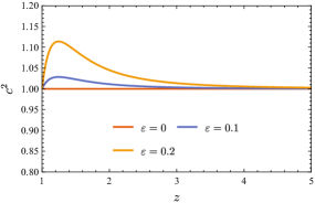
(a) Squared speed

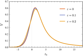
(b) Potential

Figure 1: Plot of the squared propagation speed $c^{2}$ as a function of $z$ and the potential $V$ as a function of $z_{*}$ for $\lambda=2$. Note that the coordinate $z_{*}$ is defined up to a constant which, in this plot, differs from the choice in (49). In the figure, the constant is chosen such that $z_{*}=0$ when $z=1+W(e^{-1})$, where $W$ is the Lambert function. This corresponds to the definition $z_{*}=z+\ln(z-1)$ in the GR case ($\varepsilon=0$).

Noting that $c$ tends to $1$ and $V$ vanishes both at the horizon and at spatial infinity, the asymptotic behaviour of (17) is simply given by

$$\derivative[2]{\hat{Y}_{1}}{z_{*}}+\Omega^{2}\hat{Y}_{1}\,\simeq\,0\,,$$ (53)

where we have rescaled the frequency according to

$$\Omega={\omega}\,{r_{h}}\,.$$ (54)

As a consequence, at spatial infinity, using (50), the asymptotic solution is

$$\hat{Y}_{1}\simeq\mathcal{A}_{\infty}e^{+i\Omega z}z^{i\Omega\quantity(1+{\varepsilon^{2}}/{3})}+\mathcal{B}_{\infty}e^{-i\Omega z}z^{-i\Omega\quantity(1+{\varepsilon^{2}}/{3})}\,,$$ (55)

while the solution near the horizon takes the form,

$$\hat{Y}_{1}\simeq\mathcal{A}_{\text{hor}}(z-1)^{+i\Omega\left(1-{21}\varepsilon^{2}/10\right)}+\mathcal{B}_{\text{hor}}(z-1)^{-i\Omega\left(1-{21}\varepsilon^{2}/10\right)}\,,$$ (56)

where we have used (51) when we replace $z_{*}$ by its expression in terms of $z$. Finally, the constants $\mathcal{A}_{\infty}$, $\mathcal{B}_{\infty}$, $\mathcal{A}_{\text{hor}}$ and $\mathcal{B}_{\text{hor}}$ can be fixed or partially fixed by appropriate boundary conditions.

III.4 Axial modes: first order system and asymptotics

In this subsection, we show that the asymptotic solutions, obtained previously in (55) and (56) from the Schrödinger-like equation, can be recovered directly from the first-order system which corresponds to (9) with the definitions (44). We will be making use of the algorithm presented in Langlois:2021xzq .

III.4.1 First order system and asymptotics: brief review and notations

The goal of the algorithm is to find a set of functions so that the original system is reexpressed in the simpler form

$$\derivative{\tilde{Y}}{x}=\tilde{M}\tilde{Y}\,,\qquad\tilde{M}=x^{p}\sum_{i=0}^{N}D_{i}x^{i}+\mathcal{O}(x^{N+1})\,,$$ (57)

where the matrices $D_{i}$ are diagonal and $x$ is a new variable, defined such that the asymptotic limit considered corresponds to $x\rightarrow+\infty$. For spatial infinity, we simply use $x=z$, whereas we choose $x=1/(z-1)$ for the near horizon limit $z\to 1$.

More precisely, we start with the system

$$\derivative{Y}{x}=MY\,,$$ (58)

whose matrix $M$ is immediately obtained from (9) with (44), then we make the change of variable from $z$ to $x$ if necessary, and finally the algorithm described in Langlois:2021xzq provides us with the transfer matrix $\tilde{P}$ defining the appropriate change of functions

$$Y=\tilde{P}\,\tilde{Y}\,,$$ (59)

so that the new matrix $\tilde{M}$, given by

$$\tilde{M}=\tilde{P}^{-1}M\tilde{P}-\tilde{P}^{-1}\,\derivative{\tilde{P}}{x}\,,$$ (60)

takes the diagonal form (57). Hence, we obtain immediately the asympotic behaviour of the solution by integrating the diagonal first-order differential system (57). We apply this procedure in turn to the spatial infinity and near horizon limits, up to order $\varepsilon^{2}$.

III.4.2 Spatial infinity

At spatial infinity, the coordinate variable is $z$ and the first terms of the initial matrix $M$ in an expansion in power of $z$ read

$$M=\begin{pmatrix}0&-i\Omega^{2}\\ -i&0\end{pmatrix}+\begin{pmatrix}2&0\\ -2i\quantity(1+{\varepsilon^{2}}/{3})&0\end{pmatrix}\frac{1}{z}+\mathcal{O}\quantity(\frac{1}{z^{2}})\,.$$ (61)

Applying the change of functions (59) with

$$\tilde{P}=\begin{pmatrix}\Omega&-\Omega\\ 1&1\end{pmatrix}+\frac{1}{6\Omega}\begin{pmatrix}3i\Omega-(3+\varepsilon^{2})\Omega^{2}&3i\Omega+(3+\varepsilon^{2})\Omega^{2}\\ -3i+(3+\varepsilon^{2})\Omega&3i+(3+\varepsilon^{2})\Omega\end{pmatrix}\frac{1}{z}\,,$$ (62)

provided by the algorithm of Langlois:2021xzq , one obtains the new matrix

$$\tilde{M}=\text{diag}(-i\Omega,i\Omega)+\frac{1}{z}\text{diag}\left[1-i\Omega\quantity(1+\frac{\varepsilon^{2}}{3}),1-+i\Omega\quantity(1+\frac{\varepsilon^{2}}{3})\right]+\mathcal{O}\quantity(\frac{1}{z^{2}})\,,$$ (63)

which is diagonal up to order $1/z^{2}$. Hence, the corresponding system can immediately be integrated and we find the behaviour of $Y$ and of the metric coefficients (6) at infinity:

$$h_{0}(z) \simeq\Omega\left[-c_{+}e^{i\Omega z}z^{+i\Omega\quantity(1+{\varepsilon^{2}}/{3})}+c_{-}e^{-i\Omega z}z^{-i\Omega\quantity(1+{\varepsilon^{2}}/{3})}\right]\,,$$

$$h_{c}(z) \simeq c_{+}e^{i\Omega z}z^{+i\Omega\quantity(1+{\varepsilon^{2}}/{3})}+c_{-}e^{-i\Omega z}z^{-i\Omega\quantity(1+{\varepsilon^{2}}/{3})}\,,$$ (64)

where $c_{\pm}$ are the integration constants. As expected, one recovers the same combination of modes as in (55).

III.4.3 Near the horizon

To study the asymptotic behaviour near the horizon, it is convenient to use the coordinate $x$ defined by $x=1/(z-1)$. Then, we study the behaviour, when $x$ goes to infinity, of the system (129), reformulated as

$$\derivative{Y}{x}=M_{x}(x)\,Y\,,\mbox{\quad with\quad}M_{x}(x)=-\frac{1}{x^{2}}M(1+1/x)\,.$$ (65)

The expansion of the matrix $M_{x}$ in powers of $x^{-1}$ yields

$$M_{x} = \begin{pmatrix}0&0\\ i\quantity(1-{21}/{5}\varepsilon^{2})&0\end{pmatrix}+\begin{pmatrix}0&0\\ 2i\quantity(1-{121}/{15}\varepsilon^{2})&1\end{pmatrix}\frac{1}{x}$$ (67)

$$+\frac{1}{15}\begin{pmatrix}-30-244\varepsilon^{2}&15i\Omega^{2}\\ 15i(1+1111\varepsilon^{2})&-15-662\varepsilon^{2}\end{pmatrix}\frac{1}{x^{2}}+\mathcal{O}\quantity(\frac{1}{x^{3}})\,.$$

The algorithm provides us with the transfer matrix

$$\tilde{P}=\begin{pmatrix}0&0\\ 1&1\end{pmatrix}x+\Omega\begin{pmatrix}-1-{21}\varepsilon^{2}/{10}&1+{21}\varepsilon^{2}/{10}\\ 0&0\end{pmatrix}\\ +\begin{pmatrix}2(i+\Omega)+{\varepsilon^{2}}(10i-53\Omega)/15&2(i-\Omega)+{\varepsilon^{2}}(10i+53\Omega)/15\\ 0&0\end{pmatrix}\frac{1}{x}+\mathcal{O}\quantity(\frac{1}{x^{2}})\,,$$ (68)

and one obtains a new differential system with a diagonal matrix $\tilde{M}_{x}$,

$$\tilde{M}_{x}=\frac{1}{x}\text{diag}\left[-i\Omega\quantity(1-\frac{21}{10}\varepsilon^{2}),i\Omega\quantity(1-\frac{21}{10}\varepsilon^{2})\right]+\mathcal{O}\quantity(\frac{1}{x^{2}})\,.$$ (69)

Integrating the system immediately yields the near-horizon behaviour of the metric components, expressed in terms of the variable $z$,

$$h_{0}(z) \simeq\Omega\quantity(1+{21}\varepsilon^{2}/10)\left[c_{+}(z-1)^{-1-i\Omega\quantity(1-{21}\varepsilon^{2}/10)}-c_{-}(z-1)^{-1+i\Omega\quantity(1-{21}\varepsilon^{2}/10)}\right]\,,$$

$$h_{c}(z) \simeq c_{+}(z-1)^{-1-i\Omega\quantity(1-{21}\varepsilon^{2}/10)}+c_{-}(z-1)^{-1+i\Omega\quantity(1-{21}\varepsilon^{2}/10)}\,,$$ (70)

where $c_{\pm}$ are integration constants (different from those introduced in (64)). As expected, we recover the combination of modes found in (56) from the Schrödinger-like formulation.

III.5 Polar modes

For polar modes, there is no obvious Schrödinger-like formulation of the equations of motion so the simplest approach is to work directly with the first-order system. The latter can be written in the form

$$\derivative{Y}{r}=S\,Y\,,\mbox{\quad with\quad}Y={}^{t}\!\begin{pmatrix}K,&\delta\varphi,&H_{1},&H_{0}\end{pmatrix}\,,$$ (71)

but the matrix $S$ is singular in the GR limit when $\varepsilon\to 0$. This problem can be avoided by using the functions

$$\chi=\varepsilon\,\delta\varphi\mbox{\quad and\quad}Y={}^{t}\!\begin{pmatrix}K,&\chi,&H_{1},&H_{0}\end{pmatrix}\,,$$ (72)

leading to a well-defined system in the GR limit of the form

$$\derivative{Y}{z}=M(z)\,Y\,,$$ (73)

where $z$ is the dimensionless coordinate introduced in (43). We now consider in turn the two asymptotic limits.

III.5.1 Spatial infinity

We start by computing the expansion of $M$ in powers of $z$; we obtain

$$M=M_{-2}\,z^{2}+M_{-1}\,z+M_{0}+\frac{M_{1}}{z}+\mathcal{O}\quantity(\frac{1}{z^{2}})\,.$$ (74)

The matrices $M_{-2}$, $M_{-1}$ and $M_{0}$ take the simple expressions

$$M_{-2}=\begin{pmatrix}0&0&0&0\\ a&0&0&0\\ 0&0&0&0\\ 0&0&0&0\end{pmatrix}\,,\qquad M_{-1}=\begin{pmatrix}0&0&0&0\\ a+\varepsilon^{2}\Omega^{2}/6&0&a/i\Omega&0\\ 0&0&0&0\\ 0&0&0&0\end{pmatrix}\,,$$ (75)

$$M_{0}=\begin{pmatrix}0&0&0&0\\ a\quantity(1-{\lambda}/{\Omega^{2}})-{\varepsilon^{2}\Omega^{2}}/{3}&0&0&a{\lambda}/{\Omega^{2}}\\ -i\Omega&0&0&-i\Omega\\ 0&0&-i\Omega&0\end{pmatrix}\,,$$ (76)

which depend on the coefficient $a$ defined by

$$a=-\frac{\Omega^{2}}{2}+\frac{73}{120}\rho_{2}\Omega^{2}\varepsilon+\frac{\Omega^{2}\left(13201\rho_{2}^{2}+62555\rho_{3}+209160\right)}{151200}\,\varepsilon^{2}\mbox{\quad and\quad}\rho_{3}=\frac{f^{\prime\prime\prime}(\psi_{\infty})}{f^{\prime}(\psi_{\infty})}\,,$$ (77)

while $\rho_{2}$ has been defined in (41). The matrices $M_{i}$ with $i\geq 1$ are more involved than the three above matrices and we do not give their expressions here. Nonetheless, some of them enter in the algorithm briefly recalled earlier, in section III.4.1, which enables us to diagonalise the differential system (73).

The asymptotical diagonal form at infinity cannot immediately be obtained from equation (73), as the leading order matrix $M_{-2}$ is nilpotent. As discussed in Langlois:2021xzq , for this special subcase of the algorithm, one must first obtain a diagonalisable leading order term, by applying a change of functions parametrised by the matrix

$$P^{(1)}=\mathrm{diag}(z^{-2},1,z^{-2},z^{-2})\,,$$ (78)

which gives a new matrix $M^{(1)}$, as in (60), whose leading order term is now diagonalisable. The diagonalisation of the leading term can be performed using the transformation,

$$P^{(2)}=\begin{pmatrix}0&-1&0&-1\\ 0&-i{a}/{\Omega}&0&i{a}/{\Omega}\\ 1&0&-1&0\\ 1&1&1&1\end{pmatrix}\,,$$ (79)

which yields a matrix $M^{(2)}$ of the form

$$M^{(2)}=M_{0}^{(2)}+M_{1}^{(2)}z^{-1}+{\cal O}\left(\frac{1}{z^{2}}\right)\,,\qquad M_{0}^{(2)}=\text{diag}(-i\Omega,+i\Omega,-i\Omega,+i\Omega)\,.$$ (80)

One thus finds four modes propagating at speed $c=1$, two ingoing and two outgoing modes. We expect them to be associated with the scalar and polar gravitational degrees of freedom.

In order to discriminate between the scalar and gravitational modes, it is useful to pursue the diagonalisation up to the next-to-leading order. This can be done by following, step by step, the algorithm of Langlois:2021xzq , which leads us to introduce the successive matrices $P^{(3)}$ and $P^{(4)}$,

$$P^{(3)}=I_{4}+\frac{i}{2\Omega z}\begin{pmatrix}0&0&-1&-2\\ 0&0&1&-(1+2\Omega^{2})\\ 1&2&0&0\\ -1&1-2\Omega^{2}&0&0\end{pmatrix}\,,\qquad P^{(4)}=\begin{pmatrix}-3a+b&1&0&0\\ 1&0&0&0\\ 0&0&-3a+b^{*}&1\\ 0&0&1&0\end{pmatrix}\,,$$

with the complex coefficient $b$ defined by

$$b=-\frac{1}{2}+\frac{\varepsilon^{2}}{24}i\Omega(1-3\Omega^{2}-36i\Omega)\,.$$ (81)

Hence, we obtain a new vector $Y^{(4)}$ whose corresponding matrix $M^{(4)}$ is given by

$$M^{(4)} = \text{diag}(-i\Omega,-i\Omega,i\Omega,i\Omega)$$ (82)

$$+ \frac{1}{z}\text{diag}\quantity(-1-i\Omega,3-i\Omega\quantity(1+{\varepsilon^{2}}/{3}),-1+i\Omega,3+i\Omega\quantity(1+{\varepsilon^{2}}/{3}))+{\cal O}\left(\frac{1}{z^{2}}\right)\,,$$

up to order $\varepsilon^{2}$. As a consequence, we can now easily integrate the equation for $Y^{(4)}$ up to sub-leading order when $z\gg 1$ (up to $\varepsilon^{2}$) and we obtain

$${}^{t}Y^{(4)}\simeq\begin{pmatrix}c_{-}\,\mathfrak{s}^{\infty}_{-}(z)\,,\quad d_{-}\,\mathfrak{g}^{\infty}_{-}(z)\,,\quad c_{+}\,\mathfrak{s}^{\infty}_{+}(z)\,,\quad d_{+}\,\mathfrak{g}^{\infty}_{+}(z)\end{pmatrix}\,,$$ (83)

where $c_{\pm}$ and $d_{\pm}$ are integration constants while

$$\mathfrak{g}^{\infty}_{\pm}(z)\simeq e^{\pm i\Omega z}z^{3\pm i\Omega\quantity(1+{\varepsilon^{2}}/{3})}=e^{\pm iz_{*}}\,,\qquad\mathfrak{s}^{\infty}_{\pm}(z)\simeq e^{\pm i\Omega z}z^{-1\pm i\Omega}\,.$$ (84)

The two modes $\mathfrak{g}^{\infty}_{\pm}$ follow the same behaviour as the axial modes obtained in (63): those can be dubbed gravitational modes, while the other two modes $\mathfrak{s}^{\infty}_{\pm}$ correspond to scalar modes.

We can then determine the behaviour of the metric perturbations $K$, $\chi$, $H_{1}$ and $H_{0}$ by combining the matrices $P^{(i)}$, with $i=1,\dots,4$ as

$$Y=P\,Y^{(4)}\quad\text{with}\;\;\qquad P=P^{(1)}P^{(2)}P^{(3)}P^{(4)}\,.$$ (85)

with the leading order terms of each coefficient of $P$ given by

$$P\simeq\frac{1}{z^{2}}\begin{pmatrix}-{1}&-\dfrac{1}{2iz\Omega}&-{1}&\dfrac{1}{2iz\Omega}\\ -\dfrac{iaz^{2}}{\Omega}&\dfrac{az}{2\Omega^{2}}&\frac{iaz^{2}}{\Omega}&\dfrac{az}{2\Omega^{2}}\\ {-3a+b}&{1}&{3a-b}&-{1}\\ {-3a-b}&{1}&-{(3a+b^{*})}&-{1}\end{pmatrix}\,.$$ (86)

Hence, the metric and the scalar perturbations are non-trivial linear combinations of the so-called gravitational and scalar modes. This shows that the metric and the scalar variables are dynamically entangled.

III.5.2 Near the horizon

The asymptotic behaviour of polar perturbations near the horizon is technically more complex to analyse than the previous case because we need more steps to “diagonalise” the matrix M and then to integrate asymptotically the system for the perturbations. However, the procedure is straightforward following the algorithm presented in Langlois:2021xzq . For this reason, we do not give the details of the calculation but instead present the final result.

After several changes of variables, one obtains a first order differential system satisfied by a vector $\tilde{Y}$ whose corresponding matrix $\tilde{M}$ is of the form

$$\tilde{M}=\frac{1}{z-1}\tilde{M}_{{}_{-1}}+{\cal O}\left(1\right)\,,$$ (87)

where the leading order term $M_{{}_{-1}}$ is, up to $\varepsilon^{2}$, given by

$$\tilde{M}_{{}_{-1}}=\text{diag}\left[-i\Omega\quantity(1-\frac{21}{10}\varepsilon^{2}),+i\Omega\quantity(1-\frac{21}{10}\varepsilon^{2}),-i\Omega\quantity(1-\frac{21}{10}\varepsilon^{2}),+i\Omega\quantity(1-\frac{21}{10}\varepsilon^{2})\right]+\mathcal{O}(\varepsilon^{3})\;.$$ (88)

One recognises that the coefficients of $M_{{}_{-1}}$ correspond to the leading order term in the asymptotic expansion of $\pm i\Omega z_{*}$ around $z=1$, given in (51). Indeed, we see that

$$\tilde{M}=i\Omega\,\frac{\differential z_{*}}{\differential z}\,\text{diag}\left(-1,+1,-1,+1\right)+{\cal O}(1)\,,$$ (89)

and then integrating the equation for $\tilde{Y}$ becomes trivial as

$$\frac{\differential\tilde{Y}}{\differential z_{*}}\simeq\,\text{diag}\left(-i\Omega,+i\Omega,-i\Omega,+i\Omega\right)\tilde{Y}\,,$$ (90)

which leads to the solution

$${}^{t}\tilde{Y}=(c_{-}\mathfrak{p}^{1}_{-}(z)\,,\quad c_{+}\mathfrak{p}^{1}_{+}(z)\,,\quad d_{-}\mathfrak{p}^{1}_{-}(z)\,,\quad d_{+}\mathfrak{p}^{1}_{+}(z)\,)\,,$$ (91)

where $c_{\pm}$ and $d_{\pm}$ are integration constants, and we introduced the polar modes (up to $\varepsilon^{2}$),

$$\mathfrak{p}^{1}_{\pm}(z)\simeq e^{\pm i\Omega z_{*}}=(z-1)^{\pm i\Omega(1-21\varepsilon^{2}/10)}\,.$$ (92)

Several remarks are in order. First, exactly as in the analysis of the asymptotics at infinity, one cannot discriminate between the gravitational mode and the scalar mode at leading order since they are equivalent at this order. Going to next-to-leading orders would be needed in order to further characterise each mode. Then, computing the behaviour of each mode at the horizon in terms of the metric perturbation functions, in a similar way to what was done at spatial infinity, is possible but not enlightening since the expressions are very involved. Finally, notice that the results above (84) and (92) are consistent with the behaviours found in Blazquez-Salcedo:2016enn , as one can see in their equation (17), and Minamitsuji:2022mlv as one can see in their equations (6.62) and (6.63).

IV 4d Einstein-Gauss-Bonnet black hole

In this section, we study another modified theory of gravity that involves the Gauss-Bonnet invariant $\mathcal{G}$ defined in (25). Its action is given by

$$S[g_{\mu\nu},\phi]=\int\differential[4]{x}\sqrt{-g}\left(R+\alpha(\phi\mathcal{G}+4E^{\mu\nu}\phi_{\mu}\phi_{\nu}-4X\square\phi+2X^{2})\right)\,,$$ (93)

where $\alpha$ is a constant and $E^{\mu\nu}$ the Einstein tensor. This action can be obtained as the $4D$ limit, in some specific sense, of the $D$-dimensional Einstein-Gauss-Bonnet action Lu:2020iav . As for Einstein-scalar-Gauss-Bonnet theories, this theory also belongs to degenerate scalar-tensor theories. It can be recast into a Horndeski theory with the following functions (see Appendix A):

$$P(X)=2\alpha X^{2}\,,\quad Q(X)=-4\alpha X\,,\quad F(X)=1-2\alpha X\mbox{\quad and\quad}G(X)=-4\alpha\ln X\,.$$ (94)

We will also assume that $\alpha>0$, otherwise $|\alpha|$ is constrained to be extremely small Charmousis:2021npl .

IV.1 Background solution

Let us now consider static spherically symmetric solutions of the form

$$\differential{s}^{2}=-A(r)\differential{t}^{2}+\frac{1}{A(r)}\differential{r}^{2}+r^{2}\differential{\Omega}^{2}\mbox{\quad and\quad}\phi=\phi(r)\,.$$ (95)

By solving the equations of motion for the metric and the scalar field derived from the action (93), one can find a simple analytical solution, as discussed in Lu:2020iav ; Hennigar:2020lsl . The metric function $A$ is given by

$$A(r)=1+\frac{r^{2}}{2\alpha}\left(1-\sqrt{1+\frac{4\alpha\mu}{r^{3}}}\right)=1-\frac{2\mu/r}{1+\sqrt{1+\frac{4\alpha\mu}{r^{3}}}}\,.$$ (96)

This reduces to the Schwarzschild metric in the limit $\alpha\rightarrow 0$, the parameter $\mu$ corresponding to twice the black hole mass in this limit.

If $\mu^{2}<4\alpha$, the solution is a naked singularity and is therefore of no interest. If $\mu^{2}\geq 4\alpha$, the solution for the metric describes a black hole and its horizons can be found by solving the equation $A(r)=0$ for $r$. This gives two roots, the largest one corresponding to the outermost horizon,

$$r_{h}=\frac{1}{2}\left({\mu}+{\sqrt{\mu^{2}-4\alpha}}\right)\,.$$ (97)

The equation for the scalar field gives two different branches:

$$\phi^{\prime}(r)=\frac{\sigma+\sqrt{A(r)}}{r\sqrt{A(r)}}\mbox{\quad with\quad}\sigma=\pm 1\,.$$ (98)

Integrating this equation in the limit where $r$ is large (i.e. $r\gg r_{h}$), one obtains

$$\phi(r)\simeq\frac{\mu}{2r}\quad\text{if}\;\sigma=-1\,,\qquad\phi(r)\simeq 2\ln\left(\frac{r}{\mu}\right)\quad\text{if}\;\sigma=+1\,.$$ (99)

Hence, the branch $\sigma=+1$ leads to a divergent behaviour of the scalar field at spatial infinity. In this branch, moreover, $\phi$ does not vanish when the black hole mass goes to zero and we will see later that the perturbations feature also a pathological behaviour. For these reasons, we will mostly restrict our analysis to the branch $\sigma=-1$.

In the following, it will be convenient to use the dimensionless quantities

$$z=\frac{r}{r_{h}}\mbox{\quad and\quad}\beta=\frac{\alpha}{r_{h}^{2}}\,.$$ (100)

According to these definitions and (97), one can replace $\mu$ by $(1+\beta)r_{h}$. Note that

$$0\leq\beta=\frac{\mu-r_{h}}{r_{h}}\leq 1\,,$$ (101)

as $0\leq r_{h}\leq\mu$. One can notice that both bounds can be reached: the case $\beta=0$ is the GR limit, while the case $\beta=1$ is an extremal black hole, as both horizons merge into one located at $r_{h}=\sqrt{\alpha}$. The parameter $\beta$ is therefore similar to the extremality parameter $Q/M$ for a charged black hole, and it is interesting to use it instead of $\alpha$ when studying the present family of black hole solutions.

Moreover, the outermost horizon is now at $z=1$ and the new metric function is

$$A(z)=1+\frac{z^{2}}{2\beta}\quantity(1-\sqrt{1+\frac{4\beta(1+\beta)}{z^{3}}})=1-\frac{2(1+\beta)}{z\left(1+\sqrt{1+\frac{4\beta(1+\beta)}{z^{3}}}\right)}\,.$$ (102)

Since $\phi^{\prime}$ depends on $\sqrt{A}$, as shown in (98), it is also convenient to introduce the new function

$$f(z)=\sqrt{A(z)}\,.$$ (103)

IV.2 Axial modes: the first order system

The dynamics of axial modes is described by a canonical system of the form (9). Substituting (94), (98), (102), (103) into the definitions (8) and (10-11) and rescaling all dimensionful quantities by the appropriate powers of $r_{h}$ to make them dimensionless (or, equivalently, working in units where $r_{h}=1$), one gets the following expressions for $\mathcal{F}$, $\Gamma$, $\Phi$ and $\Delta$ :

$$\mathcal{F} =\frac{f^{2}}{z^{2}}\quantity[z^{2}+2\beta(\sigma+f)(\sigma+f-2zf^{\prime})]\,,$$ (104)

$$\Gamma =\frac{1}{\mathcal{F}f^{2}z^{2}}\left[z^{2}-2\beta(1-f^{2})-4z\beta ff^{\prime}\right]=\frac{z^{4}-2\beta(1+\beta)z}{\mathcal{F}f^{2}z^{2}[z^{2}+2\beta(1-f^{2})]}\,,$$ (105)

$$\Phi =\frac{\mathcal{F}z^{2}}{z^{2}+2\beta(1-f^{2})}\,,\qquad\Delta=-\frac{\mathcal{F}^{\prime}}{\mathcal{F}}\,,$$ (106)

where we have used the explicit definition of $f(z)$ and the expression of its derivative

$$f^{\prime}=\frac{f^{2}-1}{zf}+\frac{3(1+\beta)}{2f[z^{2}-2\beta(f^{2}-1)]}$$ (107)

to obtain a simplified expression for $\Gamma$. Here, we have kept the parameter $\sigma$ unfixed: as we can see, it appears in the expression of $\mathcal{F}$ which means that it becomes relevant for the perturbations of the black hole solution.

In the sequel, it will be convenient to express the quantities (104)-(106) in terms of the following three functions of $z$:

$$\gamma_{1} =f\quantity[z^{2}+2\beta(\sigma+f)(\sigma+f-2zf^{\prime})]\,,$$ (108)

$$\gamma_{2} =z^{4}-2\beta(1+\beta)z\,,$$ (109)

$$\gamma_{3} =z^{2}+2\beta(1-f^{2})\,.$$ (110)

A short calculation then leads to

$$\mathcal{F}=\frac{f\gamma_{1}}{z^{2}}\,,\quad\Gamma=\frac{\gamma_{2}}{f^{3}\gamma_{1}\gamma_{3}}\mbox{\quad and\quad}\Phi=\frac{f\gamma_{1}}{\gamma_{3}}\,.$$ (111)

When we study the perturbations and their asymptotics, it is important to look at the zeros and the singularities of the expressions (111). For this reason, we quickly discuss the zeros of the functions $\gamma_{i}$. We note that, for $z>0$, the function $\gamma_{3}$, explicitly given by

$$\gamma_{3}=z^{2}\sqrt{1+\frac{4\beta(1+\beta)}{z^{3}}}\,,$$ (112)

is strictly positive and the function $\gamma_{2}$ vanishes at

$$z_{2}=\quantity[2\beta(1+\beta)]^{1/3}\,.$$ (113)

This root is only relevant in our analysis if it lies outside the horizon, i.e. when $z_{2}>1$, which is the case if $\beta\geq\beta_{c}$ with

$$\beta_{c}\equiv\frac{\sqrt{3}-1}{2}\simeq 0.366\,.$$ (114)

Hence, when $\beta<\beta_{c}$, $\gamma_{2}$ remains strictly positive outside the horizon. Let us note that at the special value $\beta=\beta_{c}$, the zeros of $f$ and $\gamma_{2}$ coincide. Finally, the position of the zeros of $\gamma_{1}$ depends on the sign of $\sigma$. If $\sigma=-1$, then $\sigma+f\leq 0$ and, since $f^{\prime}\geq 0$, the product $(\sigma+f)(\sigma+f-2zf^{\prime})$ is always positive, and therefore $\gamma_{1}>0$ outside the horizon. By contrast, if $\sigma=+1$, one finds numerically that $\gamma_{1}$ has a zero $z_{1}>1$. This is another reason (in addition to the behaviour of the scalar field at infinity discussed below (99)) to restrict our analysis to the case $\sigma=-1$.

Let us summarise. When $\beta<\beta_{c}$ and $\sigma=-1$, the functions $\gamma_{i}$ do not vanish outside the horizon and then neither of the three functions $\cal F$, $\Gamma$ and $\Phi$ vanishes or has a pole for $z>1$. Near the horizon, these functions behave as follows:

$$z\to 1:\;{\cal F}\simeq\frac{6\beta(1+\beta)}{1+2\beta}\,f\,,\quad\Gamma\simeq\frac{(1+2\beta)(1-2\beta-\beta^{2})}{6\beta(1+\beta)}\frac{1}{f^{3}}\,,\quad\Phi\simeq\frac{6\beta(1+\beta)}{1+2\beta}\,f\,,$$ (115)

with

$$f(z)=\sqrt{\frac{1-\beta}{1+2\beta}}\,\sqrt{z-1}+{\cal O}((z-1)^{3/2})\,.$$ (116)

At infinity, the behaviour is much simpler as the three functions (111) are constant and tend to $1$.

IV.3 Axial modes: Schrödinger-like formulation

As discussed in II.2, the axial perturbations obey the Schrödinger-like equation

$$\derivative[2]{\hat{Y}_{1}}{z_{*}}+\left(\frac{\Omega^{2}}{c^{2}(z)}-V(z)\right)\hat{Y}_{1}=0\,,$$ (117)

where $\derivative*{z}{z_{*}}=n(z)$ and $c^{2}=1/n^{2}\Gamma$, while the potential $V(z)$ is given by (16). The condition $\beta<\beta_{c}$ together with the choice $\sigma=-1$ ensures that $c^{2}>0$ everywhere outside the horizon.

A natural choice for $n$ is $n(z)=A(z)=f^{2}(z)$, in which case $z_{*}$ is the analog of the Schwarzschild tortoise coordinate. With this choice, one finds, according to (111),

$$c^{2}=\frac{\gamma_{1}\gamma_{3}}{f\gamma_{2}}\,.$$ (118)

The potential is then given by

$$V(z) = \frac{z^{2}A(\kappa_{1}+A\kappa_{2})}{\gamma_{2}^{2}\gamma_{3}^{4}}\,,\quad\text{with}$$ (119)

$$\kappa_{1} = 2(\lambda+1)z^{12}-3(\beta+1)z^{11}-2\beta(\beta+1)(2\lambda-7)z^{9}-18\beta(\beta+1)^{2}z^{8}$$

$$- 24\beta^{2}(\beta+1)^{2}(\lambda+1)z^{6}+54\beta^{2}(\beta+1)^{3}z^{5}+4\beta^{3}(\beta+1)^{3}(20\lambda-7)z^{3}$$

$$- 12\beta^{3}(\beta+1)^{4}z^{2}-8\beta^{4}(\beta+1)^{4}(8\lambda-1)\,,$$

$$\kappa_{2} = 30\beta(\beta+1)z^{9}+126\beta^{2}(\beta+1)^{2}z^{6}+108\beta^{3}(\beta+1)^{3}z^{3}+12\beta^{4}(\beta+1)^{4}\,.$$

The propagation speed and the potential for $\lambda=2$ are represented in Fig. (2) for three different values of $\beta$, satisfying the condition $\beta<\beta_{c}$.

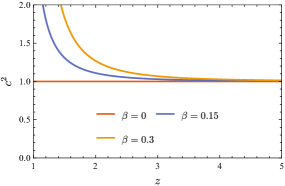
(a) Squared speed

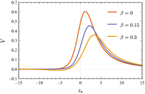
(b) Potential

Figure 2: Plot of the squared speed $c^{2}$ and the potential $V$ for $\lambda=2$. We choose the integration constant in the computation of $z_{*}$ through the same procedure as explained in Fig. (1).

We observe that the propagation speed diverges at the horizon $z=1$, while the potential vanishes at this point. The potential can be negative in some region for sufficiently large values of $\beta$. It is difficult to study analytically the sign of the potential but one can compute its derivative when $z_{*}\to-\infty$ and one finds that it remains positive up to some value $\beta_{*}(\lambda)$. We find that $\beta_{*}(\lambda=2)\simeq 0.162917$ numerically and that $\beta_{*}(\lambda\to\infty)=\beta_{c}$.

In terms of the new coordinate $z_{*}$, the Schrödinger-like equation is of the form

$$-\derivative[2]{\hat{Y}_{1}}{z_{*}}+V(z)\chi=w(z)\,\Omega^{2}\hat{Y}_{1}\,,\qquad w=f^{4}\Gamma\,.$$ (120)

The left-hand side of this equation can be seen as an operator acting on the space of functions that are square-integrable with respect to the measure $w\,\differential{z_{*}}$. It is instructive to study the asymptotic behaviour of the solutions of (120), near the horizon and at spatial infinity.

Near the horizon, using $\differential{z_{*}}=\differential{z}/f^{2}$ and (116), one finds

$$z_{*}\simeq\frac{1+2\beta}{1-\beta}\ln({z-1})\;\Longleftrightarrow\;z-1\simeq e^{\eta z_{*}}\,,\quad\eta\equiv\frac{1-\beta}{1+2\beta}\ \,,\quad(z\to 1\quad\text{or}\quad z_{*}\to-\infty)$$ (121)

and the asymptotic behaviours for the potential and for $w$ are

$$V(z)\simeq C_{1}(z-1),\qquad w(z)\simeq\frac{1-2\beta-2\beta^{2}}{2\beta\sqrt{(1-\beta)(1+2\beta)}}\sqrt{z-1}\,,$$ (122)

where $C_{1}$ is a constant. It is immediate to rewrite these asymptotic expressions in terms of $z_{*}$, using (121).

Near the horizon, for $z_{*}\to-\infty$, the potential decays faster than the right-hand side of (120) so that the differential equation takes the form

$$-\derivative[2]{\hat{Y}_{1}}{z_{*}}+C_{1}e^{\eta z_{*}/2}\hat{Y}_{1}\simeq 0\,,$$ (123)

whose solutions are

$$\hat{Y}_{1}\simeq A_{1}I_{0}\left(\frac{2}{\eta}C_{1}^{1/2}e^{\eta z_{*}/4}\right)+A_{2}K_{0}\left(\frac{2}{\eta}C_{1}^{1/2}e^{\eta z_{*}/4}\right)\,,\qquad(z_{*}\to-\infty)$$ (124)

where $I_{0}$ and $K_{0}$ are the modified Bessel functions of order $0$ while $A_{1}$ and $A_{2}$ are integration constants.

Since $I_{0}(u)\simeq 1$ and $K_{0}(u)\simeq-\ln u$ when $u\to 0$, the general solution behaves as an affine function of $z_{*}$ when $z_{*}\to-\infty$ and is therefore square integrable with respect to the measure $w\,dz_{*}\simeq e^{\eta z_{*}/2}dz_{*}$. This means that the endpoint $z_{*}\to-\infty$ is of limit circle type (according to the standard terminology, see e.g. krallSingularSelfadjointSturmLiouville1988 ). Interestingly, the analysis of the axial modes near the horizon in our case is very similar to that near a naked singularity as discussed in Sadhu:2012ur . In contrast with the GR case, none of the two axial modes is ingoing or outgoing, which means that the stability analysis of these perturbations differs from the GR one.

For the other endpoint (at spatial infinity), $z_{*}\simeq z\to+\infty$, the asymptotic behaviours of the potential $V$ and the functions $w$, according to (119) and (118), are given by

$$V(z)\simeq\frac{2(\lambda+1)}{z^{2}}\,,\qquad w(z)\simeq 1\,,$$ (125)

which coincides with the GR behaviour at spatial infinity. In particular, $V$ goes to zero and $w$ goes to one, so that one recovers the usual combination of ingoing and outgoing modes

$$\hat{Y}_{1}\simeq B_{1}e^{i\Omega z_{*}}+B_{2}e^{-i\Omega z_{*}}\,,\qquad(z_{*}\to+\infty)\,,$$ (126)

where $B_{1}$ and $B_{2}$ are constant. If $\Omega$ contains a nonzero imaginary part, then one of the modes is normalisable and then this endpoint is now of limit-point type.

As we have already said previously, the analysis of axial perturbations in this theory is very different from the analysis in GR. The main reason is that we no longer have a distinction between ingoing and outgoing modes at the horizon. The choice of the right behaviour to consider might be guided by regularity properties of the mode. Indeed, if we require the perturbation $\hat{Y}_{1}$ to be regular when $z_{*}\to-\infty$, then we have to impose $A_{2}=0$. The problem turns into a Sturm-Liouville problem, which implies that $\Omega^{2}$ is real. A very similar problem has been studied in another context in Sadhu:2012ur where the authors showed that $\Omega^{2}>0$ when $V>0$, which implies that the perturbations are stable. Here we can make the same analysis as in Sadhu:2012ur , and we expect the stability result to be true at least in the case where $V>0$, i.e. when $\beta$ is sufficiently small, as explained in the discussion below (119).

Let us close this subsection with a final remark. It is always possible to use, instead of the tortoise coordinate, a different coordinate $z_{*}$, for example by choosing $n(z)$ such that $c=1$ everywhere. This corresponds to the choice

$$n(z)=\frac{1}{\sqrt{\Gamma}}\,.$$ (127)

In this new frame, the potential is changed and can be written in the form

$$V_{c=1}=\frac{Q(f)}{16z^{2}f\gamma_{1}\gamma_{2}^{3}\gamma_{3}^{5}}\,,$$ (128)

where $Q$ is a polynomial of order 28 of nonzero constant term whose coefficients depend on $z$. This potential is represented on Fig.(3) for different values of $\beta$.

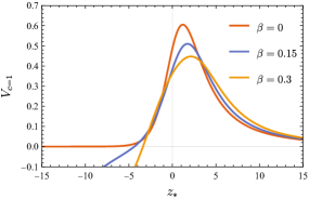
Figure 3: Plot of the potential $V_{c=1}$ for $\lambda=2$.

IV.4 Axial modes: first-order asymptotic approach

In this section, we compute the asymptotic behaviours of $h_{0}$ and $h_{c}$ using the first-order system for axial perturbations given in (9) following the algorithm we developped in Langlois:2021xzq . Using (9), with (104)-(106), we start by writing this first order system in the $z$ variable:

$$\derivative{Y}{z}=M(z)\,Y\,,\mbox{\quad with\quad}Y=\begin{pmatrix}h_{0}\\ h_{c}\end{pmatrix}\,.$$ (129)

At spatial infinity, the matrix $M$ can be expanded as

$$M(z)=\begin{pmatrix}0&-i\Omega^{2}\\ -i&0\end{pmatrix}+\mathcal{O}\left(\frac{1}{z}\right)\,.$$ (130)

Therefore, the two components of $Y$ at infinity are immediately found to be a linear combination of the following two modes:

$$\mathfrak{a}^{\rm\infty}_{\pm}(z)\simeq e^{\pm i\Omega z}=e^{\pm i\omega r}\,.$$ (131)

Hence, the asymptotic behaviour of the original metric variables $h_{0}$ and $h_{c}$ are given by

$$h_{0}(z) \simeq z\Omega\left[-c_{+}e^{i\Omega z}z^{i\Omega(1+\beta)}+c_{-}e^{-i\Omega z}z^{-i\Omega(1+\beta)}\right]\,,$$

$$h_{c}(z) \simeq z\left[c_{+}e^{i\Omega z}z^{i\Omega(1+\beta)}+c_{-}e^{-i\Omega z}z^{-i\Omega(1+\beta)}\right]\,,$$ (132)

where $c_{\pm}$ are constants.

Near the horizon, we change variables by setting $x=1/\sqrt{z-1}$, and study the behaviour, when $x$ goes to infinity, of the system (129), rewritten as

$$\derivative{Y}{x}=M_{x}(x)\,Y\,,\mbox{\quad with\quad}M_{x}(x)=-\frac{2}{x^{3}}M(1+1/x^{2})\,.$$ (133)

The algorithm then enables us to simplify the original system, here up to order $x^{-1}$, using the transfer matrix $P$ such that

$$P=\frac{1}{xp_{3}}\begin{pmatrix}p_{1}+xp_{2}&p_{2}\\ 0&x^{2}p_{3}\end{pmatrix}\,,$$ (134)

with the functions $p_{i}$ defined by

$$p_{1}=(1-\beta)^{2}\quantity(1+2\beta+6\beta^{2})\,,\quad p_{2}=2(1-\beta)^{2}\beta\sqrt{1+\beta-2\beta^{2}}\,,$$

$$p_{3}=2i(1+2\beta)^{2}(1-2\beta(1+\beta))\,.$$ (135)

The new system is then

$$\derivative{\tilde{Y}}{x}=\tilde{M}_{x}\,\tilde{Y}\,,\qquad\text{with}\quad\tilde{M}_{x}=\begin{pmatrix}0&0\\ 1/x&0\end{pmatrix}+\mathcal{O}\quantity(\frac{1}{x^{2}})\,.$$ (136)

Therefore, the solution near the horizon (written in terms of the original variable $z$) is a linear combination of two “modes”,

$$\mathfrak{a}^{\rm h}_{1}(z)\simeq 1\mbox{\quad and\quad}\mathfrak{a}^{\rm h}_{2}(z)\simeq-\frac{1}{2}\ln(z-1)\,.$$ (137)

Going back to the original variables $h_{0}$ and $h_{c}$, we get

$$h_{0}(z) \simeq\frac{p_{2}}{p_{3}}c_{1}+\sqrt{z-1}\quantity(\frac{p_{1}}{p_{3}}c_{1}+\frac{p_{2}}{p_{3}}c_{2}-\frac{p_{2}}{2p_{3}}c_{1}\ln(z-1))\,,$$

$$h_{c}(z) \simeq\frac{1}{\sqrt{z-1}}\quantity(c_{2}-\frac{1}{2}c_{1}\ln(z-1))\,,$$ (138)

with $c_{1}$ and $c_{2}$ two constants. This result is consistent with the asymptotic solution we found from the Schrödinger-like equation (124) when we expand the Bessel functions in power series.

IV.5 Polar modes

In order to compute the asymptotical behaviour of the polar modes, we proceed similarly to section IV.4. We start by writing the system as $\derivative*{Y}{z}=M(z)Y$, with $Y={}^{t}\!\begin{pmatrix}K,&\delta\varphi,&H_{1},&H_{0}\end{pmatrix}$ and $M$ is now a 4-dimensional matrix. We then compute the series expansion of the matrix $M$ at the horizon and at infinity, and apply the algorithm in order to diagonalise the system up to order $x^{-1}$ in each case using a change of vector $Y=\tilde{P}\tilde{Y}$. The matrix $\tilde{P}$ being much more involved than in the axial case, we do not give it explicitly here.

IV.5.1 Spatial infinity

At spatial infinity, the diagonalized matrix $\tilde{M}$ is found to be

$$\tilde{M}(z) = \text{diag}(0,0,-i\Omega,i\Omega)$$ (139)

$$+ \frac{1}{z}\text{diag}\left[-5-i\sqrt{\lambda},-5+i\sqrt{\lambda},1-i\Omega(1+\beta),1+i\Omega(1+\beta)\right]+\mathcal{O}\left(\frac{1}{z^{2}}\right)\,.$$

This leads to an asymptotic solution where $Y$ is a combination of 4 modes, where we recognise two polar gravitational modes,

$$\mathfrak{g}^{\rm\infty}_{\pm}(z)\simeq e^{\pm i\Omega z}z^{1\pm i\Omega(1+\beta)}\,,$$ (140)

and identify the other two as scalar modes,

$$\mathfrak{s}^{\rm\infty}_{\pm}(z)\simeq z^{-5\pm i\sqrt{\lambda}}\,.$$ (141)

We can recover the behaviour of the metric perturbations $K$, $\delta\varphi$, $H_{1}$ and $H_{0}$ which are the components of $Y$ by using the explicit expression of the matrix $\tilde{P}$. After a direct calculation, we find the following behaviour for $Y$ when $z$ goes to infinity:

$$Y\simeq\begin{pmatrix}\dfrac{-i}{\Omega z}&\dfrac{i}{\Omega z}&\dfrac{2-i\sqrt{\lambda}-\lambda}{\Omega^{2}}z&\dfrac{2+i\sqrt{\lambda}-\lambda}{\Omega^{2}}z\\ \xi&\xi^{*}&\dfrac{z^{6}}{24\beta(1+\beta)}&\dfrac{z^{6}}{24\beta(1+\beta)}\\ -1&1&\dfrac{2-i\sqrt{\lambda}}{i\Omega}z^{2}&\dfrac{2+i\sqrt{\lambda}}{i\Omega}z^{2}\\ 1&1&\dfrac{2}{3}z^{3}&\dfrac{2}{3}z^{3}\end{pmatrix}\begin{pmatrix}c_{+}\mathfrak{g}^{\rm\infty}_{+}\\ c_{-}\mathfrak{g}^{\rm\infty}_{-}\\ d_{+}\mathfrak{s}^{\rm\infty}_{+}\\ d_{-}\mathfrak{s}^{\rm\infty}_{-}\end{pmatrix}\,,$$ (142)

where

$$\xi=\frac{i(53\lambda-4)}{48\beta(\beta+1)\Omega^{3}}+\frac{57\lambda+466}{576\beta\Omega^{2}}+\frac{26327i(\beta+1)}{2304\beta\Omega}-\frac{175\beta^{2}-1954\beta+175}{36864\beta}\,.$$ (143)

and $c_{\pm}$ and $d_{\pm}$ are constants.

This result calls for a few comments. First, we can see from (141) that the scalar modes are not propagating at infinity: even though it is possible to identify two branches corresponding to two sign choices, the corresponding modes do not contain exponentials, and the leading order depends on $\lambda$. This implies that there is no choice of $z_{*}$ such that $\mathfrak{s}^{\infty}_{\pm}(z_{*})\simeq e^{\pm iz_{*}/c_{0}}$, with $c_{0}$ a constant speed independant of $\lambda$. Such a behaviour for scalar modes leads to the conclusion that defining quasinormal modes of the scalar sector in the usual way (through outgoing boundary conditions at infinity) for this solution is not possible.

Second, one can compare the asymptotic behaviour of the scalar modes with what is obtained by considering only scalar perturbations onto a fixed background; this is done in Appendix C and we see that the two behaviours are very similar, even though they slightly differ. Third, one can observe that the 4-dimensional matrix above (142) is ill-defined in the GR limit where $\beta\to 0$. In fact, the second line of the matrix tends to infinity in this limit. This could be expected, since in that limit there is no degree of freedom associated with the scalar perturbation, which is obtained precisely from the second line of the matrix. One could solve this problem by setting $\chi=\beta\,\delta\varphi$ and considering the vector ${}^{t}\!\begin{pmatrix}K,&\chi,&H_{1},&H_{0}\end{pmatrix}$, similarly to what was done for the EsGB solution in (72).

IV.5.2 Near the horizon

Near the horizon, we use the variable $x=1/\sqrt{z-1}$, as for axial modes. Using the algorithm, we find a change of vector $Y=\tilde{P}\tilde{Y}$ such that the associated matrix, that we denote $\tilde{M}_{x}$ exactly as in (133), is diagonal and is explicitly given by

$$\tilde{M}_{x}=\frac{1}{x}\,\text{diag}(-1,0,0,2)+\mathcal{O}\quantity(\frac{1}{x^{2}})\,.$$ (144)

Solving the first order system is then immediate and the asymptotic expressions of the components of the 4-dimensional vector $\tilde{Y}$ (written as functions of $z$) are combinations of the four modes

$$\mathfrak{g}^{\rm h}_{1}(z)\simeq 1\,,\quad\mathfrak{g}^{\rm h}_{2}(z)\simeq\frac{1}{z-1}\,,\quad\mathfrak{s}^{\rm h}_{1}(z)\simeq 1\mbox{\quad and\quad}\mathfrak{s}^{\rm h}_{2}(z)\simeq\sqrt{z-1}\,.$$ (145)

We have named two of these modes $\mathfrak{s}_{i}$ (for “scalar”) because they contain a nonzero $\delta\varphi$ contribution, as can be seen by expressing these modes in terms of the original perturbative quantities, using the explicit expression for the matrix $\tilde{P}$ provided by the algorithm. Indeed, the relation between each of the above modes and the initial perturbations is given by

$$Y\simeq\begin{pmatrix}\dfrac{\zeta_{1}}{\sqrt{z-1}}&\zeta_{2}\sqrt{z-1}&\zeta_{4}\sqrt{z-1}&\zeta_{6}\sqrt{z-1}\\ 0&0&1&\sqrt{z-1}\\ \dfrac{1}{z-1}&1&0&\zeta_{7}\sqrt{z-1}\\ 0&\dfrac{\zeta_{3}}{\sqrt{z-1}}&\dfrac{\zeta_{5}}{\sqrt{z-1}}&\zeta_{8}\end{pmatrix}\begin{pmatrix}c_{1}\,\mathfrak{g}^{\rm h}_{1}\\ c_{2}\,\mathfrak{g}^{\rm h}_{2}\\ d_{1}\,\mathfrak{s}^{\rm h}_{1}\\ d_{2}\,\mathfrak{s}^{\rm h}_{2}\end{pmatrix}\,,$$ (146)

where $c_{i}$ and $d_{i}$ are integration constants while $\zeta_{i}$ are constants whose expressions are given explicitly in Appendix B.

This behaviour is similar to what we have obtained for the axial perturbations. One cannot exhibit ingoing and outgoing modes: instead, the perturbations have non-oscillating behaviours at the horizon.

V Conclusion

In this work, we have studied the linear perturbations about black hole solutions in the context of two families of gravity theories involving a Gauss-Bonnet term in the action. In order to do so we have extended our previous work to the case of Horndeski theories with a cubic dependence on second derivatives of the scalar field, since the Gauss-Bonnet models studied here can be recast in the form of scalar-tensor theories (we show explicitly, in Appendix A, the equivalence between the Lagrangians with the Gauss-Bonnet term and the corresponding scalar-tensor Lagrangians following what has been done in colleauxRegularBlackHole2019 ).

For a general shift-symmetric Horndeski theory, we have written the expression for the equations of motion of the axial perturbations about any static spherically symmetric background in a simple and compact form. The axial perturbations represent a single degree of freedom and their dynamics can be described either by a two-dimensional first-order (in radial derivatives) system or by a Schrödinger-like second-order equation, associated with a potential and a propagation speed. By contrast, the polar modes, which describe the coupled even-parity gravitational degree of freedom and the scalar field degree of freedom, are characterized by a four-dimensional first-order system. We then apply this general formalism to the two models considered here.

For Einstein-scalar-Gauss-Bonnet theories, one difficulty is that there is no exact background black hole solution. The solution can be computed numerically or analytically in a perturbative expansion. We have followed the second approach here, following Julie:2019sab and providing some details about the calculation of the lowest order metric terms. We have then studied the perturbations, up to second order in the small expansion parameter (related to the coupling of the Gauss-Bonnet term). We have tackled the axial modes using both the Schrödinger reformulation and the first-order system approach, thus cross-checking our results. As for polar modes, we have applied our algorithm to determine their asymptotic behaviours. We have found that both axial and polar modes have a rather standard behaviour. In particular, one can immediately see the existence of ingoing and outgoing modes at both boundaries and one can easily distinguish in most cases gravitational and scalar degrees of freedom at the boundaries.

In the last part of this work, we have considered the perturbations of the 4dGB black hole solution of Lu:2020iav , for the first time to our knowledge. The Schrödinger reformulation of the equations of motion for the axial modes is characterised by the unusual property that the propagation speed diverges at the horizon (using the tortoise coordinate as radial coordinate), even if the potential vanishes in this limit. We also find a critical value $\beta_{c}$ for the coupling beyond which the square of the propagation speed becomes negative. Studying the case $\beta<\beta_{c}$, we have found that the asymptotic behaviour at spatial infinity is very similar to that of Schwarzschild but the modes are very peculiar near the horizon. These results are confirmed by our first-order approach.

Moreover, concerning both polar and axial perturbations, it is not possible to apply the usual classification of modes into ingoing/outgoing categories near the horizon. Furthermore, we prove that the scalar modes have a leading order behaviour at infinity that strongly depends on the angular momentum, which seems to imply that no scalar waves propagate at infinity.

In summary, we have illustrated in this work how our formalism can be used in a straightforward and systematic way to study the asymptotic behaviours of the perturbations about a black hole solution in a large family of scalar-tensor theories. When the perturbations are well-behaved, this is a useful starting point for the numerical computation of the quasi-normal modes. By contrast, if the perturbations are ill-behaved, it indicates that the solution or even the underlying gravitational theory might be pathological. In this sense, our general formalism can be used as an efficient diagnostic of the healthiness of some modified gravity theory, or at least the viability of some associated black hole solutions.

Appendix A Scalar Einstein-Gauss-Bonnet theory as cubic Horndeski

In this Appendix, we show that a coupling between a scalar field and the Gauss-Bonnet term gives, in 4-dimensional spacetimes, a cubic Horndeski theory. We use the expression of the Gauss-Bonnet term as a total derivative given in colleauxRegularBlackHole2019 and we reproduce the proof of this reference in a simpler case here. Our result was already proven in Kobayashi:2011nu , but was obtained in that case only from the equations of motion. The computation we present here is made at the level of the action.

Let us study the action

$$S_{\text{GB}}[g_{\mu\nu},\phi]=\int\differential[4]{x}\sqrt{-g}f(\phi)\mathcal{G}\,,$$ (147)

with $\mathcal{G}$ the Gauss-Bonnet invariant defined by

$$\mathcal{G}=R_{\mu\nu\rho\sigma}R^{\mu\nu\rho\sigma}-4R_{\mu\nu}R_{\mu\nu}+R^{2}\,.$$ (148)

In 4 dimensions, the Lagrangian density $\sqrt{-g}\,\mathcal{G}$ is a total derivative: therefore integration by parts should allow us to recover a scalar-tensor action from (147). It is proven in Crisostomi:2017ugk that the Einstein-Gauss-Bonnet action completed with a kinetic term for the scalar field contains only one scalar degree of freedom. It is therefore expected that the action (147) can be written as a specific case of (1).

We use the expression of $\mathcal{G}$ as a total derivative given in colleauxRegularBlackHole2019 : introducing an arbitrary field $\phi$, one has

$$\mathcal{G}=-2\delta^{\mu\nu\alpha\beta}_{\sigma\rho\lambda\delta}\nabla^{\delta}\quantity[\frac{\tensor{\phi}{{}_{\alpha}^{\lambda}}\phi_{\beta}}{X}\quantity(\tensor{R}{{}_{\mu}{}_{\nu}^{\sigma}{}^{\rho}}+\frac{4}{3}\frac{\tensor{\phi}{{}_{\mu}^{\sigma}}\tensor{\phi}{{}_{\nu}^{\rho}}}{X})]\,,$$ (149)

where we introduced the tensor

$$\delta^{\mu\nu\alpha\beta}_{\sigma\rho\lambda\delta}=-\varepsilon^{\mu\nu\alpha\beta}\varepsilon_{\sigma\rho\lambda\delta}\,.$$ (150)

The idea of the proof done in colleauxRegularBlackHole2019 is to generate Riemann terms by using the commutation of covariant derivatives acting on $\phi^{\mu}$, using the formula

$$\commutator{\nabla_{\mu}}{\nabla_{\nu}}\phi^{\rho}=\tensor{R}{{}^{\rho}_{\lambda}{}_{\mu}{}_{\nu}}\phi^{\lambda}\,.$$ (151)

In order to obtain the squared Riemann terms present in $\mathcal{G}$, one searches an expression of $\mathcal{G}$ in the schematic form $\nabla_{\mu}(\phi_{\nu\rho}\phi_{\sigma}R_{\lambda\delta\alpha\beta})$. The action of the covariant derivative on $\phi_{\nu\rho}$ will lead to a squared Riemann term as expected. Recovering the Gauss-Bonnet will require antisymmetrization, since one has

$$\mathcal{G}=\frac{1}{4}\delta^{\mu\nu\alpha\beta}_{\sigma\rho\lambda\delta}\tensor{R}{{}_{\mu}{}_{\nu}^{\sigma}{}^{\rho}}\tensor{R}{{}_{\alpha}{}_{\beta}^{\lambda}{}^{\delta}}\,.$$ (152)

We will therefore contract the expression with the fully antisymmetric tensor. However, several new terms will be created when the covariant derivative acts on the other parts of the expression: specific tuning of prefactors in front of these terms will be required to make sure only the Gauss-Bonnet invariant is left in the end.

We reproduce the proof in colleauxRegularBlackHole2019 in the specific case of 4-dimensional spacetime. We start from the generic Lagrangian

$$L=\delta^{\mu\nu\alpha\beta}_{\sigma\rho\lambda\delta}\nabla^{\delta}\quantity[a_{0}\frac{\tensor{\phi}{{}_{\alpha}^{\lambda}}\phi_{\beta}}{X}\tensor{R}{{}_{\mu}{}_{\nu}^{\sigma}{}^{\rho}}+a_{1}\frac{\tensor{\phi}{{}_{\alpha}^{\lambda}}\phi_{\beta}}{X^{2}}\tensor{\phi}{{}_{\mu}^{\sigma}}\tensor{\phi}{{}_{\nu}^{\rho}}]\,,$$ (153)

where $a_{0}$ and $a_{1}$ are constants. By expanding the covariant derivative $\nabla^{\delta}$ in $L$, one obtains

$$L=a_{0}\delta^{\mu\nu\alpha\beta}_{\sigma\rho\lambda\delta}\quantity[\frac{\nabla^{\delta}\tensor{\phi}{{}_{\alpha}^{\lambda}}}{X}\phi_{\beta}\tensor{R}{{}_{\mu}{}_{\nu}^{\sigma}{}^{\rho}}+\frac{\tensor{\phi}{{}_{\alpha}^{\lambda}}\tensor{\phi}{{}_{\beta}^{\delta}}}{X}\tensor{R}{{}_{\mu}{}_{\nu}^{\sigma}{}^{\rho}}-\frac{2}{X^{2}}\tensor{\phi}{{}_{\alpha}^{\lambda}}\tensor{\phi}{{}_{\kappa}^{\delta}}\phi^{\kappa}\phi_{\beta}\tensor{R}{{}_{\mu}{}_{\nu}^{\sigma}{}^{\rho}}]\\ +a_{1}\delta^{\mu\nu\alpha\beta}_{\sigma\rho\lambda\delta}\quantity[\frac{3}{X^{2}}\quantity(\nabla^{\delta}\tensor{\phi}{{}_{\alpha}^{\lambda}})\phi_{\beta}\tensor{\phi}{{}_{\mu}^{\sigma}}\tensor{\phi}{{}_{\nu}^{\rho}}+\frac{\tensor{\phi}{{}_{\alpha}^{\lambda}}\tensor{\phi}{{}_{\beta}^{\delta}}\tensor{\phi}{{}_{\mu}^{\sigma}}\tensor{\phi}{{}_{\nu}^{\rho}}}{X^{2}}-\frac{4}{X^{3}}\phi^{\kappa}\phi_{\beta}\tensor{\phi}{{}_{\kappa}^{\delta}}\tensor{\phi}{{}_{\alpha}^{\lambda}}\tensor{\phi}{{}_{\mu}^{\sigma}}\tensor{\phi}{{}_{\nu}^{\rho}}]\,,$$ (154)

by regrouping terms that are equal under contraction with the totally antisymmetric tensor. One notices that the covariant derivatives of the Riemann tensors disappear by application of the second Bianchi identities. By using the first Bianchi identities and eq. 151, one obtains

$$2\delta^{\mu\nu\alpha\beta}_{\sigma\rho\lambda\delta}\nabla^{\delta}\tensor{\phi}{{}_{\alpha}^{\lambda}}=-\delta^{\mu\nu\alpha\beta}_{\sigma\rho\lambda\delta}\tensor{R}{{}^{\lambda}{}^{\delta}_{\alpha}{}_{\kappa}}\phi^{\kappa}\,,$$ (155)

which allows us to write

$$L=a_{0}\quantity[-\frac{1}{2X}\Omega_{2,0}-\frac{2}{X^{2}}\Omega_{3,1}+\frac{1}{X}\Omega_{1,1}]+a_{1}\quantity[-\frac{3}{2X^{2}}\Omega_{2,1}+\frac{1}{X^{2}}\Omega_{1,2}-\frac{4}{X^{3}}\Omega_{3,2}]\,,$$ (156)

where the functions $\Omega_{i,j}$ are defined in colleauxRegularBlackHole2019 as

$$\Omega_{1,0}=\delta^{\mu\nu\alpha\beta}_{\sigma\rho\lambda\delta}\tensor{R}{{}_{\mu}{}_{\nu}^{\sigma}{}^{\rho}}\tensor{R}{{}_{\alpha}{}_{\beta}^{\lambda}{}^{\delta}}\,,\quad \Omega_{1,2}=\delta^{\mu\nu\alpha\beta}_{\sigma\rho\lambda\delta}\tensor{\phi}{{}_{\mu}^{\sigma}}\tensor{\phi}{{}_{\nu}^{\rho}}\tensor{\phi}{{}_{\alpha}^{\lambda}}\tensor{\phi}{{}_{\beta}^{\delta}}\,,$$

$$\Omega_{1,1}=\delta^{\mu\nu\alpha\beta}_{\sigma\rho\lambda\delta}\tensor{R}{{}_{\mu}{}_{\nu}^{\sigma}{}^{\rho}}\tensor{\phi}{{}_{\alpha}^{\lambda}}\tensor{\phi}{{}_{\beta}^{\delta}}\,,\quad \Omega_{3,1}=\delta^{\mu\nu\alpha\beta}_{\sigma\rho\lambda\delta}\phi_{\kappa}\phi^{\lambda}\tensor{\phi}{{}_{\alpha}^{\kappa}}\tensor{R}{{}_{\mu}{}_{\nu}^{\sigma}{}^{\rho}}\tensor{\phi}{{}_{\beta}^{\delta}}\,,$$

$$\Omega_{2,0}=\delta^{\mu\nu\alpha\beta}_{\sigma\rho\lambda\delta}\phi_{\kappa}\phi^{\rho}\tensor{R}{{}_{\mu}{}_{\nu}^{\sigma}{}^{\kappa}}\tensor{R}{{}_{\alpha}{}_{\beta}^{\lambda}{}^{\delta}}\,,\quad \Omega_{3,2}=\delta^{\mu\nu\alpha\beta}_{\sigma\rho\lambda\delta}\phi_{\kappa}\phi^{\sigma}\tensor{\phi}{{}_{\mu}^{\kappa}}\tensor{\phi}{{}_{\nu}^{\rho}}\tensor{\phi}{{}_{\alpha}^{\lambda}}\tensor{\phi}{{}_{\beta}^{\delta}}\,,$$

$$\Omega_{2,1}=\delta^{\mu\nu\alpha\beta}_{\sigma\rho\lambda\delta}\phi_{\kappa}\phi^{\rho}\tensor{R}{{}_{\mu}{}_{\nu}^{\sigma}{}^{\kappa}}\tensor{\phi}{{}_{\alpha}^{\lambda}}\tensor{\phi}{{}_{\beta}^{\delta}}\,.$$ (157)

One can then prove the following identities relating the functions $\Omega_{i,j}$:

$$X\Omega_{1,0}-4\Omega_{2,0}=\delta^{\mu\nu\alpha\beta\gamma}_{\sigma\rho\lambda\delta\kappa}\phi_{\mu}\phi^{\sigma}\tensor{R}{{}_{\nu}{}_{\alpha}^{\rho}{}^{\lambda}}\tensor{R}{{}^{\delta}{}^{\kappa}_{\beta}{}_{\gamma}}=0\,,$$

$$X\Omega_{1,1}-2\Omega_{2,1}-2\Omega_{3,1}=\delta^{\mu\nu\alpha\beta\gamma}_{\sigma\rho\lambda\delta\kappa}\phi_{\mu}\phi^{\sigma}\tensor{\phi}{{}_{\nu}^{\rho}}\tensor{\phi}{{}_{\alpha}^{\lambda}}\tensor{R}{{}^{\delta}{}^{\kappa}_{\beta}{}_{\gamma}}=0\,,$$

$$X\Omega_{1,2}-4\Omega_{3,2}=\delta^{\mu\nu\alpha\beta\gamma}_{\sigma\rho\lambda\delta\kappa}\phi_{\mu}\phi^{\sigma}\tensor{\phi}{{}_{\nu}^{\rho}}\tensor{\phi}{{}_{\alpha}^{\lambda}}\tensor{\phi}{{}_{\beta}^{\delta}}\tensor{\phi}{{}_{\gamma}^{\kappa}}=0\,,$$ (158)

since in 4 dimensions the fully antisymmetric tensor $\delta^{\mu\nu\alpha\beta\gamma}_{\sigma\rho\lambda\delta\kappa}$ is zero (there are more indices than dimensions so two indices have to be repeated). Eq. (156) then becomes

$$L=-\frac{a_{0}}{8}\Omega_{1,0}+\frac{\Omega_{2,1}}{X^{2}}\quantity(2a_{0}-\frac{3}{2}a_{1})\,.$$ (159)

One can see from (157) and (152) that $\Omega_{1,0}=4\mathcal{G}$. Therefore, by choosing $a_{0}=-2$ and $a_{1}=4a_{0}/3=-8/3$, one obtains (149).

We can now use the expression of $\mathcal{G}$ as a total derivative to express the action (147) as a Horndeski theory. Injecting this relation into Eq. (147) and integrating by parts gives

$$S_{\text{GB}}[g_{\mu\nu},\phi]=\int\differential[4]{x}\sqrt{-g}\frac{2}{X}\derivative{f}{\phi}\delta^{\mu\nu\alpha\beta}_{\sigma\rho\lambda\delta}\tensor{\phi}{{}_{\alpha}^{\lambda}}\phi_{\beta}\phi^{\delta}\quantity(\tensor{R}{{}_{\mu}{}_{\nu}^{\sigma}{}^{\rho}}+\frac{4}{3}\frac{\tensor{\phi}{{}_{\mu}^{\sigma}}\tensor{\phi}{{}_{\nu}^{\rho}}}{X})\,.$$ (160)

After expanding the products, one finds that the Lagrangian density $L_{\mathcal{G}}$ of (160) is

$$L_{\mathcal{G}}=-\derivative{f}{\phi}\begin{multlined}\Big{[}8R^{\mu\nu}\phi_{\mu\nu}+\frac{4}{X}\phi^{\mu}\phi_{\mu\nu}\phi^{\nu}-4R\Box\phi-\frac{16}{X}\tensor{R}{{}_{\mu}^{\nu}}\phi^{\mu}\phi^{\rho}\phi_{\nu\rho}-\frac{16}{3X}\tensor{\phi}{{}_{\mu}^{\nu}}\phi^{\mu\rho}\phi_{\rho\nu}\\ +\frac{8}{X}\Box\phi\phi_{\mu\nu}\phi^{\mu\nu}+\frac{16}{X^{2}}\phi^{\mu}\phi^{\nu}\tensor{\phi}{{}_{\mu}^{\rho}}\tensor{\phi}{{}_{\nu}^{\sigma}}\phi_{\rho\sigma}+\frac{8}{X}R_{\mu\nu}\phi^{\mu}\phi^{\nu}\Box\phi\\ -\frac{8}{3X}(\Box\phi)^{3}-\frac{8}{X}R_{\mu\nu\rho\sigma}\phi^{\mu}\phi^{\nu}\phi^{\rho\sigma}-\frac{8}{X^{2}}\phi^{\mu}\phi_{\mu\nu}\phi^{\nu}\phi_{\rho\sigma}\phi^{\rho\sigma}\\ -\frac{16}{X^{2}}\phi^{\mu}\phi^{\nu}\tensor{\phi}{{}_{\mu}^{\rho}}\phi_{\rho\nu}\Box\phi+\frac{8}{X^{2}}\phi^{\mu}\phi_{\mu\nu}\phi^{\nu}(\Box\phi)^{2}\Big{]}\,.\end{multlined}\Big{[}8R^{\mu\nu}\phi_{\mu\nu}+\frac{4}{X}\phi^{\mu}\phi_{\mu\nu}\phi^{\nu}-4R\Box\phi-\frac{16}{X}\tensor{R}{{}_{\mu}^{\nu}}\phi^{\mu}\phi^{\rho}\phi_{\nu\rho}-\frac{16}{3X}\tensor{\phi}{{}_{\mu}^{\nu}}\phi^{\mu\rho}\phi_{\rho\nu}\\ +\frac{8}{X}\Box\phi\phi_{\mu\nu}\phi^{\mu\nu}+\frac{16}{X^{2}}\phi^{\mu}\phi^{\nu}\tensor{\phi}{{}_{\mu}^{\rho}}\tensor{\phi}{{}_{\nu}^{\sigma}}\phi_{\rho\sigma}+\frac{8}{X}R_{\mu\nu}\phi^{\mu}\phi^{\nu}\Box\phi\\ -\frac{8}{3X}(\Box\phi)^{3}-\frac{8}{X}R_{\mu\nu\rho\sigma}\phi^{\mu}\phi^{\nu}\phi^{\rho\sigma}-\frac{8}{X^{2}}\phi^{\mu}\phi_{\mu\nu}\phi^{\nu}\phi_{\rho\sigma}\phi^{\rho\sigma}\\ -\frac{16}{X^{2}}\phi^{\mu}\phi^{\nu}\tensor{\phi}{{}_{\mu}^{\rho}}\phi_{\rho\nu}\Box\phi+\frac{8}{X^{2}}\phi^{\mu}\phi_{\mu\nu}\phi^{\nu}(\Box\phi)^{2}\Big{]}\,.$$ (161)

One can recognise several total derivatives:

$$\nabla_{\mu}\quantity(\frac{1}{X})=-\frac{2}{X^{2}}\phi^{\nu}\phi_{\mu\nu}\mbox{\quad and\quad}\nabla_{\mu}(\ln(X))=\frac{2}{X}\phi^{\nu}\phi_{\mu\nu}\,.$$ (162)

integrating by parts the terms containing these total derivatives and writing contractions of the Riemann tensors as commutators of derivatives, one obtains

$$L_{\mathcal{G}}=\begin{multlined}\derivative{f}{\phi}\quantity[-E_{\mu\nu}\phi^{\mu\nu}(8+4\ln(X))-\frac{4}{3X}(L_{1}^{(3)}-3L_{2}^{(3)}+2L_{3}^{(3)})]\\ +\derivative[2]{f}{\phi}\quantity[2X\ln(X)R+4\ln(X)L_{1}^{(2)}+4(L_{1}^{(2)}-L_{2}^{(2)})]\\ +2\derivative[3]{f}{\phi}X(1-3\ln(X))\Box\phi-2\derivative[4]{f}{\phi}X^{2}\ln(X)\,,\end{multlined}\derivative{f}{\phi}\quantity[-E_{\mu\nu}\phi^{\mu\nu}(8+4\ln(X))-\frac{4}{3X}(L_{1}^{(3)}-3L_{2}^{(3)}+2L_{3}^{(3)})]\\ +\derivative[2]{f}{\phi}\quantity[2X\ln(X)R+4\ln(X)L_{1}^{(2)}+4(L_{1}^{(2)}-L_{2}^{(2)})]\\ +2\derivative[3]{f}{\phi}X(1-3\ln(X))\Box\phi-2\derivative[4]{f}{\phi}X^{2}\ln(X)\,,$$ (163)

where the $L_{i}^{(j)}$ are the DHOST Lagrangians introduced in BenAchour:2016fzp :

$$L_{1}^{(2)}=\phi_{\mu\nu}\phi^{\mu\nu}\,,\quad L_{2}^{(2)}=(\Box\phi)^{2}\,,$$

$$L_{1}^{(3)}=(\Box\phi)^{3}\,,\quad L_{2}^{(3)}=(\Box\phi)\phi_{\mu\nu}\phi^{\mu\nu}\,,\quad L_{3}^{(3)}=\phi_{\mu\nu}\phi^{\nu\rho}\phi^{\mu}_{\rho}\,.$$ (164)

Finally, one can rewrite the term $E_{\mu\nu}\phi^{\mu\nu}$ using $\nabla^{\mu}E_{\mu\nu}=0$ and writing contractions of the Ricci as commutators of derivatives, yielding

$$\int\differential[4]{x}\sqrt{-g}E_{\mu\nu}\phi^{\mu\nu}\derivative{f}{\phi}=\int\differential[4]{x}\sqrt{-g}\Big{[}\frac{1}{2}R\derivative[2]{f}{\phi}+2(L_{1}^{(2)}-L_{2}^{(2)})\derivative[2]{f}{\phi}\\ -3X\Box\phi\derivative[3]{f}{\phi}-4X^{2}\derivative[4]{f}{\phi}\Big{]}\,.$$ (165)

Putting Eq. (165) into Eq. (163), one finally concludes that the action (147) is equivalent to a cubic Horndeski theory with

$$G(\phi,X)=-4\derivative{f}{\phi}\ln(X)\,,\quad F(\phi,X)=-2X(2-\ln(X))\derivative[2]{f}{\phi}\,,$$

$$Q(\phi,X)=2X(7-3\ln(X))\derivative[3]{f}{\phi}\,,\quad P(\phi,X)=2X^{2}(3-\ln(X))\derivative[4]{f}{\phi}\,.$$ (166)

This direct proof, which does not exist in the literature to the best of our knowledge, complements the indirect proof given in Kobayashi:2011nu based on the equivalence of the equations of motion.

Appendix B Asymptotic behaviour near the horizon for the 4dEGB black hole

In this Appendix, we give the explicit value of the coefficients $\zeta_{1}$ up to $\zeta_{8}$ appearing in (146):

$$\zeta_{1} =-\frac{4i(2\beta+1)\sqrt{-2\beta^{2}+\beta+1}\Omega}{4(2\beta\Omega+\Omega)^{2}+(\beta-1)^{2}}\,,$$

$$\zeta_{2} =-\frac{4i\sqrt{1-\beta}}{(2\beta+1)^{3/2}\Omega\nu}\Big{[}\!\begin{multlined}(\beta-1)^{2}\left(6\beta^{2}-2\beta-1\right)(2\beta+1)^{3}\Omega^{2}\\ +(\beta-1)^{4}\beta(\beta(2\beta(8\lambda-1)+8\lambda-5)+1)\\ +4(2\beta(\beta+1)-1)(2\beta+1)^{5}\Omega^{4}\Big{]}\,,\end{multlined}(\beta-1)^{2}\left(6\beta^{2}-2\beta-1\right)(2\beta+1)^{3}\Omega^{2}\\ +(\beta-1)^{4}\beta(\beta(2\beta(8\lambda-1)+8\lambda-5)+1)\\ +4(2\beta(\beta+1)-1)(2\beta+1)^{5}\Omega^{4}\Big{]}\,,$$ (170)

$$\zeta_{3} =-\frac{2i(1-\beta)^{3/2}\beta}{\sqrt{2\beta+1}(2\beta(\beta+1)-1)\Omega}\,,$$

$$\zeta_{4} =\frac{4(1-\beta)^{3/2}}{\sqrt{2\beta+1}\nu}\Big{[}\!\begin{multlined}(\beta-1)^{2}(2\beta(4\beta(\beta(3\lambda-1)+\lambda-2)+2\lambda+1)+1)\\ -4(2\beta(4\beta(\beta\lambda+\lambda+1)-2\lambda+1)-1)(2\beta\Omega+\Omega)^{2}\Big{]}\,,\end{multlined}(\beta-1)^{2}(2\beta(4\beta(\beta(3\lambda-1)+\lambda-2)+2\lambda+1)+1)\\ -4(2\beta(4\beta(\beta\lambda+\lambda+1)-2\lambda+1)-1)(2\beta\Omega+\Omega)^{2}\Big{]}\,,$$ (173)

$$\zeta_{5} =\frac{4\sqrt{1-\beta}\beta\sqrt{2\beta+1}}{2\beta(\beta+1)-1}\,,$$

$$\zeta_{6} =\frac{8(\beta-1)^{2}\beta}{4(2\beta+1)^{3}\Omega^{2}+(\beta-1)^{2}(6\beta+1)}\,,$$

$$\zeta_{7} =\frac{8i\beta\Omega\left(12(\beta+1)(2\beta+1)^{3}\Omega^{2}+(\beta-1)^{2}(\beta(10\beta+13)+7)\right)}{12(\beta-1)(2\beta+1)^{4}\Omega^{2}+3(\beta-1)^{3}(6\beta+1)(2\beta+1)}\,,$$

$$\zeta_{8} =\frac{4(\beta-1)\beta\left(4(2\beta\Omega+\Omega)^{2}+(\beta-1)^{2}\right)}{\sqrt{-2\beta^{2}+\beta+1}\left(4(2\beta+1)^{3}\Omega^{2}+(\beta-1)^{2}(6\beta+1)\right)}\,,$$ (174)

with

$$\nu=(2\beta(\beta+1)-1)\left(4(2\beta\Omega+\Omega)^{2}+(\beta-1)^{2}\right)^{2}\,.$$ (175)

Appendix C Asymptotical behaviour for the scalar field

In this Appendix, we study the linear perturbations of the scalar field about a fixed background. This corresponds to a “decoupling limit”, in which metric perturbations are zero and only the scalar field perturbations stay dynamical.

C.1 Effective potential

Let us consider the equation for the scalar field perturbation of the form

$$c_{2}(r)\delta\varphi^{\prime\prime}(r)+c_{1}(r)\delta\varphi^{\prime}(r)+c_{0}(r)\delta\varphi(r)=0\,.$$ (176)

We aim to obtain the asymptotical behaviour of $\delta\varphi$ near some value $r_{0}$ of $r$, for example $r_{0}=+\infty$. It is not possible to take directly the limit $r\longrightarrow r_{0}$ for each coefficient $c_{i}$, since one does not know in general how the first and second derivative of $\delta\varphi$ scale with respect to each other.

One therefore changes variables in order to obtain a simpler equation. Let us write

$$\delta\varphi(r)=\kappa(r)\chi(r)\,,$$ (177)

and we have

$$c_{2}\kappa\derivative[2]{\chi}{r}+\quantity(2\kappa^{\prime}c_{2}+\kappa c_{1})\derivative{\chi}{r}+\quantity(\kappa^{\prime\prime}c_{2}+\kappa^{\prime}c_{1}+\kappa c_{0})=0\,.$$ (178)

One can then get rid of the first derivative by imposing

$$\frac{\kappa^{\prime}}{\kappa}=-\frac{c_{1}}{2c_{2}}\,.$$ (179)

The equation becomes

$$\derivative[2]{\chi}{r}+\quantity(\frac{\kappa^{\prime\prime}}{\kappa}+\frac{c_{1}}{c_{2}}\frac{\kappa^{\prime}}{\kappa}+\frac{c_{0}}{c_{2}})\chi=0\,.$$ (180)

Using (179) allows us to find the relation

$$\frac{\kappa^{\prime\prime}}{\kappa}=\frac{c_{2}^{\prime}c_{1}-c_{2}c_{1}^{\prime}}{2c_{2}^{2}}-\frac{c_{1}}{2c_{2}}\frac{\kappa^{\prime}}{\kappa}=\frac{c_{2}^{\prime}c_{1}-c_{2}c_{1}^{\prime}}{2c_{2}^{2}}+\quantity(\frac{c_{1}}{2c_{2}})^{2}\,,$$ (181)

which finally leads to the equation,

$$-\derivative[2]{\chi}{r}+V_{\chi}(r)\chi=0\mbox{\quad with\quad}V_{\chi}(r)=\frac{c_{2}c_{1}^{\prime}-c_{2}^{\prime}c_{1}}{2c_{2}^{2}}+\quantity(\frac{c_{1}}{2c_{2}})^{2}-\frac{c_{0}}{c_{2}}\,.$$ (182)

In order to obtain the behaviour near $r_{0}$, one can then decompose $V_{\chi}(r)$ around $r_{0}$ and solve directly for $\chi$. The solution will be the expansion of $\chi$ around $r_{0}$. One must then come back to $\delta\varphi$ by using Eqs. (179) and (177).

C.2 Application to the 4D Einstein-Gauss-Bonnet black hole

The equation of motion for a scalar perturbation $\delta\varphi(t,r)$ with the metric perturbation fixed to zero is

$$c_{2}(r)\partialderivative[2]{\delta\varphi}{r}+c_{1}(r)\partialderivative{\delta\varphi}{r}+c_{0}(r)\delta\varphi=0\,,$$ (183)

with

$$c_{0}(r) =\frac{8\alpha\ell(\ell+1)}{r^{2}}\quantity(4\sigma A+2\sqrt{A}A-2r\sigma A^{\prime}+\sqrt{A}(2-2rA^{\prime}+r^{2}A^{\prime\prime}))\,,$$ (184)

$$c_{1}(r) =8\alpha\quantity(4\sqrt{A}A^{\prime}-r\sigma A^{\prime 2}+\sigma A(4A^{\prime}-2rA^{\prime\prime}))\,,$$ (185)

$$c_{2}(r) =-16\alpha\sqrt{A}\quantity(2A+2\sigma A\sqrt{A}-r\sigma\sqrt{A}A^{\prime})\,.$$ (186)

We observe that time does not appear in the equations and $\delta\varphi$ satisfies an elliptic equation rather than the expected hyperbolic equation. The fact that $\delta\varphi$ does not propagate could be related a strong coupling problem.

Applying the reasoning presented in the previous section, one finds that the asymptotical behaviour of $\delta\varphi$ is

$$\delta\varphi=Ar^{-i\sqrt{1+\lambda}}+Br^{+i\sqrt{1+\lambda}}\,.$$ (187)

We do not recover exactly the asymptotical behaviour found in (141) where both metric and scalar perturbations have been considered. However, the behaviours are very similar. This result differs from the solutions studied in Langlois:2021aji , for which the behaviour of the decoupled scalar perturbations and the scalar mode found from the full system agreed at both the horizon and infinity. It can be seen as the effect of a more important backreaction of the scalar field onto the metric. One can note that the behaviours still agree in the $\lambda\longrightarrow+\infty$ limit, implying that the coupling between the metric and the scalar perturbations becomes subdominant in that case.

Appendix D Equations of motion for the background and for axial perturbations

The variation of the shift-symmetric Horndeski action (1) yields the equations of motion

$${\cal B}_{\mu\nu}\equiv\frac{\delta S}{\delta g_{\mu\nu}}=0\,,\qquad{\cal B}_{\phi}\equiv\frac{\delta S}{\delta\phi}=0\,.$$ (188)

Due to Bianchi identities, the equation for the scalar field is not independent from the metric equations and therefore can be ignored. For a metric of the form (2) and a scalar field profile (3), one finds that there are only four non-trivial equations which are given in a supplementary Mathematica notebook.

Given any background metric $\tensor{\overline{g}}{{}_{\mu}{}_{\nu}}$ solution to the above equations, one can introduce the perturbed metric

$$\tensor{g}{{}_{\mu}{}_{\nu}}=\tensor{\overline{g}}{{}_{\mu}{}_{\nu}}+\tensor{h}{{}_{\mu}{}_{\nu}}\,,$$ (189)

where the $\tensor{h}{{}_{\mu}{}_{\nu}}$ denotes the linear perturbations of the metric. In order to derive the linear equations of motion that govern the evolution of $h_{\mu\nu}$, one expands the action (1) up to second order in $\tensor{h}{{}_{\mu}{}_{\nu}}$. The Euler-Lagrange equations associated with the quadratic part $S_{\text{quad}}$ of this expansion then provide the linearised equations of motion for $h_{\mu\nu}$. In the following, they will be written under the form $\mathcal{E}_{\mu\nu}=0$, where $\mathcal{E}_{\mu\nu}$ is defined by

$$\mathcal{E}_{\mu\nu}=\functionalderivative{S_{\text{quad}}}{h_{\mu\nu}}\,.$$ (190)

In the Regge-Wheeler gauge, all the components of $h_{\mu\nu}$ for $\ell\geq 2$ are expressed in terms of the independent functions $h_{0}$ and $h_{1}$, as given in (5). In this gauge, one can show that the equations of motion reduce to the three equations $\mathcal{E}_{t\theta}=0$, $\mathcal{E}_{r\theta}=0$ and $\mathcal{E}_{\theta\theta}=0$. These three equations depend only on $F$ and $G$, since the terms proportional to $P$ and $Q$ and their derivatives vanish when the above background equations are imposed. They are given in the supplementary notebook as well.

As there are only two independent functions, $h_{0}$ and $h_{1}$, one expects one of the above equations to be redundant. This is indeed verified by noting the following relation between the equations and their derivatives:

$$\derivative{\mathcal{E}_{r\theta}}{r}-\frac{i\omega}{AB}\mathcal{E}_{t\theta}+\frac{B^{\prime}}{B}\mathcal{E}_{r\theta}+\frac{\lambda}{r^{2}B}\mathcal{E}_{\theta\theta}=0\,.$$ (191)

This shows that the two equations $\mathcal{E}_{r\theta}=0$ and $\mathcal{E}_{\theta\theta}=0$ are sufficient to fully describe the dynamics of axial perturbations. Finally, these two equations can be formulated as a simple first order system, given in (9).

References

• (1) D. Langlois and K. Noui, “Degenerate higher derivative theories beyond Horndeski: Evading the Ostrogradski instability,” Journal of Cosmology and Astroparticle Physics 2016 (Feb., 2016) 034–034, 1510.06930.
• (2) D. Langlois and K. Noui, “Hamiltonian analysis of higher derivative scalar-tensor theories,” JCAP 1607 (2016), no. 07 016, 1512.06820.
• (3) M. Crisostomi, K. Koyama, and G. Tasinato, “Extended Scalar-Tensor Theories of Gravity,” Journal of Cosmology and Astroparticle Physics 2016 (Apr., 2016) 044–044, 1602.03119.
• (4) J. B. Achour, M. Crisostomi, K. Koyama, D. Langlois, K. Noui, and G. Tasinato, “Degenerate higher order scalar-tensor theories beyond Horndeski up to cubic order,” Journal of High Energy Physics 2016 (Dec., 2016) 100, 1608.08135.
• (5) G. W. Horndeski, “Second-order scalar-tensor field equations in a four-dimensional space,” Int.J.Theor.Phys. 10 (1974) 363–384.
• (6) T. Kobayashi, H. Motohashi, and T. Suyama, “Black hole perturbation in the most general scalar-tensor theory with second-order field equations I: The odd-parity sector,” Physical Review D 85 (Apr., 2012) 084025, 1202.4893.
• (7) T. Kobayashi, H. Motohashi, and T. Suyama, “Black hole perturbation in the most general scalar-tensor theory with second-order field equations II: The even-parity sector,” Physical Review D 89 (Apr., 2014) 084042, 1402.6740.
• (8) H. Ogawa, T. Kobayashi, and T. Suyama, “Instability of hairy black holes in shift-symmetric Horndeski theories,” Physical Review D 93 (Mar., 2016) 064078, 1510.07400.
• (9) K. Takahashi and T. Suyama, “Linear perturbation analysis of hairy black holes in shift-symmetric Horndeski theories: Odd-parity perturbations,” Physical Review D 95 (Jan., 2017) 024034, 1610.00432.
• (10) E. Babichev, C. Charmousis, G. Esposito-Farese, and A. Lehébel, “Hamiltonian vs stability and application to Horndeski theory,” Physical Review D 98 (Nov., 2018) 104050, 1803.11444.
• (11) K. Takahashi, H. Motohashi, and M. Minamitsuji, “Linear stability analysis of hairy black holes in quadratic degenerate higher-order scalar-tensor theories: Odd-parity perturbations,” Physical Review D 100 (July, 2019) 024041, 1904.03554.
• (12) K. Tomikawa and T. Kobayashi, “Perturbations and quasi-normal modes of black holes with time-dependent scalar hair in shift-symmetric scalar-tensor theories,” Physical Review D 103 (Apr., 2021) 084041, 2101.03790.
• (13) C. de Rham and J. Zhang, “Perturbations of Stealth Black Holes in DHOST Theories,” Physical Review D 100 (Dec., 2019) 124023, 1907.00699.
• (14) J. Khoury, M. Trodden, and S. S. C. Wong, “Existence and instability of novel hairy black holes in shift-symmetric horndeski theories,” 2007.01320.
• (15) K. Takahashi and H. Motohashi, “Black hole perturbations in DHOST theories: Master variables, gradient instability, and strong coupling,” Journal of Cosmology and Astroparticle Physics 2021 (Aug., 2021) 013, 2106.07128.
• (16) C. Charmousis, M. Crisostomi, R. Gregory, and N. Stergioulas, “Rotating Black Holes in Higher Order Gravity,” Physical Review D 100 (Oct., 2019) 084020, 1903.05519.
• (17) C. Charmousis, M. Crisostomi, D. Langlois, and K. Noui, “Perturbations of a rotating black hole in DHOST theories,” 1907.02924.
• (18) D. Langlois, K. Noui, and H. Roussille, “Asymptotics of linear differential systems and application to quasi-normal modes of nonrotating black holes,” Physical Review D 104 (Dec., 2021) 124043, 2103.14744.
• (19) D. Langlois, K. Noui, and H. Roussille, “Black hole perturbations in modified gravity,” Physical Review D 104 (Dec., 2021) 124044, 2103.14750.
• (20) H. Lu and Y. Pang, “Horndeski Gravity as $d\rightarrow 4$ Limit of Gauss-Bonnet,” Physics Letters B 809 (Oct., 2020) 135717, 2003.11552.
• (21) R. A. Hennigar, D. Kubiznak, R. B. Mann, and C. Pollack, “On Taking the $D\to 4$ limit of Gauss-Bonnet Gravity: Theory and Solutions,” Journal of High Energy Physics 2020 (July, 2020) 27, 2004.09472.
• (22) A. Colleaux, Regular Black Hole and Cosmological Spacetimes in Non-Polynomial Gravity Theories. PhD thesis, University of Trento, June, 2019.
• (23) J. L. Blázquez-Salcedo, C. F. B. Macedo, V. Cardoso, V. Ferrari, L. Gualtieri, F. S. Khoo, J. Kunz, and P. Pani, “Perturbed black holes in Einstein-dilaton-Gauss-Bonnet gravity: Stability, ringdown, and gravitational-wave emission,” Physical Review D 94 (Nov., 2016) 104024, 1609.01286.
• (24) J. L. Blázquez-Salcedo, F. S. Khoo, and J. Kunz, “Quasinormal modes of Einstein-Gauss-Bonnet-dilaton black holes,” Physical Review D: Particles and Fields 96 (2017), no. 6 064008, 1706.03262.
• (25) F.-L. Julié and E. Berti, “Post-Newtonian dynamics and black hole thermodynamics in Einstein-scalar-Gauss-Bonnet gravity,” Physical Review D 100 (Nov., 2019) 104061, 1909.05258.
• (26) C. Charmousis, A. Lehébel, E. Smyrniotis, and N. Stergioulas, “Astrophysical constraints on compact objects in 4D Einstein-Gauss-Bonnet gravity,” Journal of Cosmology and Astroparticle Physics 2022 (Feb., 2022) 033, 2109.01149.
• (27) S. Mignemi and N. R. Stewart, “Charged black holes in effective string theory,” Physical Review D 47 (June, 1993) 5259–5269, hep-th/9212146.
• (28) T. Torii, H. Yajima, and K.-i. Maeda, “Dilatonic Black Holes with Gauss-Bonnet Term,” Physical Review D 55 (Jan., 1997) 739–753, gr-qc/9606034.
• (29) N. Yunes and L. C. Stein, “Non-Spinning Black Holes in Alternative Theories of Gravity,” Physical Review D 83 (May, 2011) 104002, 1101.2921.
• (30) T. P. Sotiriou and S.-Y. Zhou, “Black hole hair in generalized scalar-tensor gravity,” Physical Review Letters 112 (June, 2014) 251102, 1312.3622.
• (31) T. P. Sotiriou and S.-Y. Zhou, “Black hole hair in generalized scalar-tensor gravity: An explicit example,” Physical Review D 90 (Dec., 2014) 124063, 1408.1698.
• (32) D. Ayzenberg and N. Yunes, “Slowly-Rotating Black Holes in Einstein-Dilaton-Gauss-Bonnet Gravity: Quadratic Order in Spin Solutions,” Physical Review D 90 (Aug., 2014) 044066, 1405.2133.
• (33) P. Pani, C. F. B. Macedo, L. C. B. Crispino, and V. Cardoso, “Slowly rotating black holes in alternative theories of gravity,” Physical Review D 84 (Oct., 2011) 087501, 1109.3996.
• (34) A. Maselli, P. Pani, L. Gualtieri, and V. Ferrari, “Rotating black holes in Einstein-Dilaton-Gauss-Bonnet gravity with finite coupling,” Physical Review D 92 (Oct., 2015) 083014, 1507.00680.
• (35) L. Hui, A. Podo, L. Santoni, and E. Trincherini, “Effective Field Theory for the Perturbations of a Slowly Rotating Black Hole,” Journal of High Energy Physics 2021 (Dec., 2021) 183, 2111.02072.
• (36) T. Kobayashi, “Horndeski theory and beyond: A review,” Reports on Progress in Physics 82 (July, 2019) 086901.
• (37) T. Kobayashi, M. Yamaguchi, and J. Yokoyama, “Generalized G-inflation: Inflation with the most general second-order field equations,” Progress of Theoretical Physics 126 (Sept., 2011) 511–529, 1105.5723.
• (38) A. Bryant, H. O. Silva, K. Yagi, and K. Glampedakis, “Eikonal quasinormal modes of black holes beyond general relativity III: Scalar Gauss-Bonnet gravity,” Physical Review D 104 (Aug., 2021) 044051, 2106.09657.
• (39) M. Minamitsuji, K. Takahashi, and S. Tsujikawa, “Linear stability of black holes in shift-symmetric Horndeski theories with a time-independent scalar field,” arXiv:2201.09687 [astro-ph, physics:gr-qc, physics:hep-th] (Jan., 2022) 2201.09687.
• (40) A. M. Krall and A. Zettl, “Singular selfadjoint Sturm-Liouville problems,” Differential and Integral Equations 1 (Jan., 1988) 423–432.
• (41) A. Sadhu and V. Suneeta, “A naked singularity stable under scalar field perturbations,” International Journal of Modern Physics D 22 (Mar., 2013) 1350015, 1208.5838.
• (42) M. Crisostomi, K. Noui, C. Charmousis, and D. Langlois, “Beyond Lovelock gravity: Higher derivative metric theories,” Physical Review D 97 (Feb., 2018) 044034, 1710.04531.