Seeded graph matching for the correlated Gaussian Wigner model via the projected power method

Abstract

In the graph matching problem we observe two graphs $G,H$ and the goal is to find an assignment (or matching) between their vertices such that some measure of edge agreement is maximized. We assume in this work that the observed pair $G,H$ has been drawn from the correlated Wigner model – a popular model for correlated weighted graphs – where the entries of the adjacency matrices of $G$ and $H$ are independent Gaussians and each edge of $G$ is correlated with one edge of $H$ (determined by the unknown matching) with the edge correlation described by a parameter $\sigma\in[0,1)$. In this paper, we analyse the performance of the projected power method (PPM) as a seeded graph matching algorithm where we are given an initial partially correct matching (called the seed) as side information. We prove that if the seed is close enough to the ground-truth matching, then with high probability, PPM iteratively improves the seed and recovers the ground-truth matching (either partially or exactly) in $\mathcal{O}(\log n)$ iterations. Our results prove that PPM works even in regimes of constant $\sigma$, thus extending the analysis in (Mao et al., 2021) for the sparse Erdös-Renyi model to the (dense) Wigner model. As a byproduct of our analysis, we see that the PPM framework generalizes some of the state-of-art algorithms for seeded graph matching. We support and complement our theoretical findings with numerical experiments on synthetic data.

1 Introduction

In the graph matching problem we are given as input two graphs $G$ and $H$ with an equal number of vertices, and the objective is to find a bijective function, or matching, between the vertices of $G$ and $H$ such that the alignment between the edges of $G$ and $H$ is maximized. This problem appears in many applications such as computer vision (H. Sun and Fei, 2020), network de-anonymization (Narayanan and Shmatikov, 2009), pattern recognition (Conte et al., 2004; Emmert-Streib et al., 2016), protein-protein interactions and computational biology (Zaslavskiy et al., 2009b; Singh et al., 2009). In computer vision, for example, it is used as a method of comparing two objects (or images) encoded as graph structures or to identify the correspondence between the points of two discretized images of the same object at different times. In network de-anonymization, the goal is to learn information about an anonymized (unlabeled) graph using a related labeled graph as a reference, exploiting their structural similarities. In (Narayanan and Shmatikov, 2006) for example, the authors show that it was possible to effectively de-anonymize the Netflix database using the IMDb (Internet Movie Database) as the “reference” network.

The graph matching problem is well defined for any pair of graphs (weighted or unweighted) and it can be framed as an instance of the NP-hard quadratic assignment problem (QAP) (Makarychev et al., 2014). It also contains the ubiquitous graph isomorphism (with unknown complexity) as a special case. However, in the average case situation, many polynomial time algorithms have recently been shown to recover, either perfectly or partially, the ground-truth vertex matching with high probability. It is thus customary to assume that the observed graphs $G,H$ are generated by a model for correlated random graphs, where the problem can be efficiently solved. The two most popular models are the correlated Correlated Erdős-Rényi model (Pedarsani and Grossglauser, 2011), where two graphs are independently sampled from an Erdős-Rényi mother graph, and the Correlated Gaussian Wigner model (Ding et al., 2021; Fan et al., 2019), which considers that $G,H$ are complete weighted graphs with independent Gaussian entries on each edge; see Section 1.3 for a precise description. Recently, other models of correlation have been proposed for random graphs with a latent geometric structure (Kunisky and Niles-Weed, 2022; Wang et al., 2022a), community structure (Rácz and Sridhar, 2021) and with power law degree profile (Yu et al., 2021a).

In this work, we will focus on the seeded version of the problem, where side information about the matching is provided (together with the two graphs $G$ and $H$) by a partially correct bijective map from the vertices of $G$ to the vertices of $H$ referred to as the seed. The quality of the seed can be measured by its overlap with the ground-truth matching. This definition of a seed is more general than what is often considered in the literature (Mossel and Xu, 2019), including the notion of a partially correct (or noisy) seed (Lubars and Srikant, 2018; Yu et al., 2021b). The seeded version of the problem is motivated by the fact that in many applications, a set of correctly matched vertices is usually available – either as prior information, or it can be constructed by hand (or via an algorithm). From a computational point of view, seeded algorithms are also more efficient than seedless algorithms (see the related work section). Several algorithms, based on different techniques, have been proposed for seeded graph matching. In (Pedarsani and Grossglauser, 2011; Yartseva and Grossglauser, 2013), the authors use a percolation-based method to “grow” the seed to recover (at least partially) the ground-truth matching. Other algorithms (Lubars and Srikant, 2018; Yu et al., 2021b) construct a similarity matrix between the vertices of both graphs and then solve the maximum linear assignment problem (either optimally or by a greedy approach) using the similarity matrix as the cost matrix. The latter strategy has also been successfully applied in the case described below when no side information is provided. Mao et al. (2021) also analyzed an iterative refinement algorithm to achieve exact recovery under the CER model with a constant level of correlation. However, all of the previously mentioned work focuses on binary (and often sparse) graphs while in a lot of applications, for example, protein-to-protein interaction networks or image matching, the graphs of interest are weighted and sometimes dense.

Contributions.

The main contributions of this paper are summarized below. To our knowledge, these are the first theoretical results for seeded weighted graph matching.

• We analyze a variant of the projected power method (PPM) for the seeded graph matching problem in the context of the CGW model. We provide (see Theorems 1, 2) exact and partial recovery guarantees under the CGW model when the PPM is initialized with a given data-independent seed, and only one iteration of the PPM algorithm is performed. For this result to hold, it suffices that the overlap of the seed with the ground-truth permutation is $\Omega(\sqrt{n\log n})$.

• We prove (see Theorem 3) that when multiple iterations are allowed, then PPM converges to the ground-truth matching in $\mathcal{O}(\log n)$ iterations provided that it is initialized with a seed with overlap $\Omega\big{(}(1-\kappa)n\big{)}$, for a constant $\kappa$ small enough, even if the initialization is data-dependent (i.e. a function of the graphs to be matched) or adversarial. This extends the results in (Mao et al., 2021) from the sparse Erdős-Rényi setting, to the dense Gaussian Wigner case.

• We complement our theoretical results with experiments on synthetic data, showing that PPM can help to significantly improve the accuracy of the matching (for the Correlated Gaussian Wigner model) compared to that obtained by a standalone application of existing seedless methods.

1.1 Notation

We denote $\mathcal{P}_{n}$ to be the set of permutation matrices of size $n\times n$ and $\mathcal{S}_{n}$ the set of permutation maps on the set $[n]=\{1,\cdots,n\}$. To each element $X\in\mathcal{P}_{n}$ (we reserve capital letters for its matrix form), there corresponds one and only one element $x\in\mathcal{S}_{n}$ (we use lowercase letters when referring to functions). We denote $\operatorname{Id}$ (resp. $\operatorname{id}$) the identity matrix (resp. identity permutation), where the size will be clear from the context. For $X\in\mathcal{P}_{n}$($x\in\mathcal{S}_{n}$), we define $S_{X}=\{i\in[n]:X_{ii}=1\}$ to be the set of fixed points of $X$, and $s_{x}=|S_{X}|/n$ its fraction of fixed points. The symbols $\langle\cdot,\cdot\rangle_{F}$, and $\|\cdot\|_{F}$ denote the Frobenius inner product and matrix norm, respectively. For any matrix $X\in\mathbb{R}^{n\times n}$, let $[X]\in\mathbb{R}^{n^{2}}$ denote its vectorization obtained by stacking its columns one on top of another. For two random variables $X,Y$ we write $X\stackrel{{\scriptstyle d}}{{=}}Y$ when they are equal in law. For a matrix $A\in\mathbb{R}^{n\times n}$, $A_{i:}$ (resp. $A_{:i}$) will denote its $i$-th row (resp. column).

1.2 Mathematical description

Let $A,B$ be the adjacency matrices of the graphs $G,H$ each with $n$ vertices. In the graph matching problem, the goal is to find the solution of the following optimization problem

$$\max_{x\in\mathcal{S}_{n}}\sum_{i,j}A_{ij}B_{x(i)x(j)}\enskip$$ (P1)

which is equivalent to solving

$$\max_{X\in\mathcal{P}_{n}}\langle A,XBX^{T}\rangle_{F}.$$ (P1’)

Observe that (P1) is a well-defined problem – not only for adjacency matrices – but for any pair of matrices of the same size. In particular, it is well-defined when $A,B$ are adjacency matrices of weighted graphs, which is the main setting of this paper. Moreover, this is an instance of the well-known quadratic assignment problem, which is a combinatorial optimization problem known to be NP-hard in the worst case (Burkard et al., 1998). Another equivalent formulation of (P1) is given by the following “lifted” (or vector) version of the problem

$$\max_{[X]\in[\mathcal{P}_{n}]}[X]^{T}(B\otimes A)[X]$$ (P1”)

where $[\mathcal{P}_{n}]$ is the set of permutation matrices in vector form. This form has been already considered in the literature, notably in the family of spectral methods (Onaran and Villar, 2017; Feizi et al., 2020).

1.3 Statistical models for correlated random graphs

Most of the theoretical statistical analysis for the graph matching problem has been performed so far under two random graph models: the Correlated Erdős-Rényi and the Correlated Gaussian Wigner model. In these models the dependence between the two graphs $A$ and $B$ is explicitly described by the inclusion of a “noise” parameter which captures the degree of correlation between $A$ and $B$.

Correlated Gaussian Wigner (CGW) model $W(n,\sigma,x^{*})$.

The problem (P1) is well-defined for matrices that are not necessarily $0/1$ graph adjacencies, so a natural extension is to consider two complete weighted graphs. The following Gaussian model has been proposed in (Ding et al., 2021)

$$A_{ij}\sim\begin{cases}\mathcal{N}(0,\frac{1}{n})\text{ if }i<j,\\ \mathcal{N}(0,\frac{2}{n})\text{ if }i=j,\end{cases}$$

$A_{ij}=A_{ji}$ for all $i,j\in[n]$, and $B_{x^{*}(i)x^{*}(j)}=\sqrt{1-\sigma^{2}}A_{ij}+\sigma Z_{ij}$, where $Z\stackrel{{\scriptstyle d}}{{=}}A$. Both $A$ and $B$ are distributed as the GOE (Gaussian orthogonal ensemble). Here the parameter $\sigma>0$ should be interpreted as the noise parameter and in that sense, $B$ can be regarded as a “noisy perturbation” of $A$. Moreover, $x^{*}\in\mathcal{S}_{n}$ is the ground-truth (or latent) permutation that we seek to recover. It is not difficult to verify that the problem (P1) is in fact the maximum likelihood estimator (MLE) of $x^{*}$ under the CGW model.

Correlated Erdős-Rényi (CER) model $G(n,q,s,x^{*})$

. For $q,s\in[0,1]$, the correlated Erdős-Rényi model with latent permutation $x^{*}\in\mathcal{S}_{n}$ can be described in two steps.

1. $A$ is generated according to the Erdős-Rényi model $G(n,q)$, i.e. for all $i<j$, $A_{ij}$ is sampled from independent Bernoulli’s r.v. with parameter $q$, $A_{ji}=A_{ij}$ and $A_{ii}=0$.

2. Conditionally on $A$, the entries of $B$ are i.i.d according to the law

   $$B_{x^{*}(i),x^{*}(j)}\sim\begin{cases}Bern(s)\quad\text{if}\quad A_{ij}=1,\\ Bern\big{(}\frac{q}{1-q}(1-s)\big{)}\quad\text{if }A_{ij}=0.\end{cases}$$ (1.1)

There is another equivalent description of this model in the literature, where to obtain CER graphs, we first sample an Erdős-Rényi “mother” graph and then define $A,B$ as independent subsamples with certain density parameter. We refer to (Pedarsani and Grossglauser, 2011) for details.

1.4 Related work

Information-theoretic limits of graph matching.

The necessary and sufficient conditions for correctly estimating the matching between two graphs when they are generated from the CGW or the CER model have been investigated in (Cullina and Kiyavash, 2017; Hall and Massoulié, 2022; Wu et al., 2021). In particular, for the CGW model, it has been shown in (Wu et al., 2021, Thm.1) that the ground truth permutation $x^{*}$ can be exactly recovered w.h.p. only when $\sigma^{2}\leq 1-\frac{(4+\epsilon)\log n}{n}$. When $\sigma^{2}\geq 1-\frac{(4-\epsilon)\log n}{n}$ no algorithm can even partially recover $x^{*}$. However, it is not known if there is a polynomial time algorithm that can reach this threshold.

Efficient algorithms

• Seedless algorithms. Several polynomial time algorithms have been proposed relying on spectral methods (Umeyama, 1988; Fan et al., 2019; Ganassali et al., 2022; Feizi et al., 2020; Cour et al., 2006), degree profiles (Ding et al., 2021; Osman Emre Dai and Grosslglauser, 2019), other vertex signatures (Mao et al., 2021), random walk based approaches (Rohit Singh and Berger, 2008; Kazemi and Grossglauser, 2016; Gori et al., 2004), convex and concave relaxations (Aflalo et al., 2015; Lyzinski et al., 2016; Zaslavskiy et al., 2009a), and other non-convex methods (Yu et al., 2018; Xu et al., 2019; Onaran and Villar, 2017). Most of the previous algorithms have theoretical guarantees only in the low noise regime. For instance, the Grampa algorithm proposed in (Fan et al., 2019) provably exactly recovers the ground truth permutation for the CGW model when $\sigma=\mathcal{O}(\frac{1}{\log n})$, and in (Ding et al., 2021) it is required for the CER (resp. CGW) model that the two graphs differ by at most $1-s=\mathcal{O}(\frac{1}{\log^{2}n})$ fraction of edges (resp. $\sigma=O(\frac{1}{\log n})$). There are only two exceptions for the CER model where the noise level is constant: the work of (Ganassali and Massoulié, 2020) and (Mao et al., 2021). But these algorithms exploit the sparsity of the graph in a fundamental manner and cannot be extended to dense graphs.

• Seeded algorithms. In the seeded case, different kinds of consistency guarantees have been proposed: consistency after one refinement step (Yu et al., 2021b; Lubars and Srikant, 2018), consistency after several refinement steps uniformly over the seed (Mao et al., 2021). For the dense CER ($p$ of constant order), one needs to have an initial seed with $\Omega(\sqrt{n\log n})$ overlap in order to have consistency after one step for a given seed (Yu et al., 2021b). But if we want to have a uniform result, one needs to have a seed that overlaps the ground-truth permutation in $O(n)$ points (Mao et al., 2021). Our results for the CGW model are similar in that respect. Besides, contrary to seedless algorithms, our algorithm works even if the the noise level $\sigma$ is constant.

Projected power method (PPM).

PPM, which is also often referred to as a generalized power method (GPM) in the literature is a family of iterative algorithms for solving constrained optimization problems. It has been used with success for various tasks including clustering SBM (Wang et al., 2021), group synchronization (Boumal, 2016; Gao and Zhang, 2022b), joint alignment from pairwise difference (Chen and Candès, 2016), low rank-matrix recovery (Chi et al., 2019) and the generalized orthogonal Procrustes problem (Ling, 2021). It is a useful iterative strategy for solving non-convex optimization problems, and usually requires a good enough initial estimate. In general, we start with an initial candidate satisfying a set of constraints and at each iteration we perform

1. a power step, which typically consists in multiplying our initial candidate with one or more data dependent matrices, and

2. a projection step where the result of the power step is projected onto the set of constraints of the optimization problem.

These two operations are iteratively repeated and often convergence to the “ground-truth signal” can be ensured in $\mathcal{O}(\log n)$ iterations, provided that a reasonably good initialization is provided.

The projected power method (PPM) has also been used to solve the graph matching problem, and its variants, by several authors. In some works, it has been explicitly mentioned (Onaran and Villar, 2017; Bernard et al., 2019), while in others (Mao et al., 2021; Yu et al., 2021b; Lubars and Srikant, 2018) very similar algorithms have been proposed without acknowledging the relation with PPM (which we explain in more detail below). All the works that study PPM explicitly do not report statistical guarantees and, to the best of our knowledge, theoretical guarantees have been obtained only in the case of sparse Erdős-Rényi graphs, such as in (Mao et al., 2021, Thm.B) in the case of multiple iterations, and (Yu et al., 2021b; Lubars and Srikant, 2018) in the case of one iteration. Interestingly, the connection with the PPM is not explicitly stated in any of these works.

2 Algorithm

2.1 Projected power method for Graph matching

We start by defining the projection operator onto $\mathcal{P}_{n}$ for a matrix $C\in\mathbb{R}^{n\times n}$. We will use the greedy maximum weight matching (GMWM) algorithm introduced in (Lubars and Srikant, 2018), for the problem of graph matching with partially correct seeds, and subsequently used in (Yu et al., 2021b). The steps are outlined in Algorithm 1.

Algorithm 1 GMWM (Greedy maximum weight matching)

1:A cost matrix $C\in\mathbb{R}^{n\times n}$.

2:A permutation matrix $X$.

3:Select $(i_{1},j_{1})$ such that $C_{i_{1},j_{1}}$ is the largest entry in $C$ (break ties arbitrarily). Define $C^{(1)}\in\mathbb{R}^{n\times n}$: $C^{(1)}_{ij}=C_{ij}\mathbbm{1}_{i\neq i_{1},j\neq j_{1}}-\infty\cdot\mathbbm{1}_{i=i_{1}\text{or }j=j_{1}}$.

4:for $k=2$ to $N$ do

5:     Select $(i_{k},j_{k})$ such that $C^{(k-1)}_{i_{k},j_{k}}$ is the largest entry in $C^{(k-1)}$.

6:     Define $C^{(k)}\in\mathbb{R}^{n\times n}$: $C^{(k)}_{ij}=C^{(k-1)}_{ij}\mathbbm{1}_{i\neq i_{k},j\neq j_{k}}-\infty\cdot\mathbbm{1}_{i=i_{k}\text{or }j=j_{k}}$.

7:end for

8:Define $X\in\{0,1\}^{n\times n}$: $X_{ij}=\sum^{N}_{k=1}\mathbbm{1}_{i=i_{k},j=j_{k}}$.

9:return $X$

Notice that the original version of GMWM works by erasing the row and column of the largest entry of the matrix $C^{(k)}$ at each step $k$. We change this to assign $-\infty$ to each element of the row and column of the largest entry (which is equivalent), mainly to maintain the original indexing. The output of Algorithm 1 is clearly a permutation matrix, hence we define

$$\tau(C):=\text{Output of GMWM with input }C$$ (2.1)

which can be considered a projection since $\tau(\tau(C))=\tau(C)$ for all $C\in\mathbb{R}^{n\times n}$. Notice that, in general, the output of GMWM will be different from solving the linear assignment problem

$$\tilde{\tau}(C):=\underset{}{\operatorname{argmin}}{\{\|C-X\|_{F}\enskip|\enskip X\in\mathcal{P}_{n}\}}=\underset{\Pi\in\mathcal{P}_{n}}{\operatorname{argmax}}{\langle\Pi,C\rangle_{F}}$$

which provides an orthogonal projection, while $\tau$ corresponds to an oblique projection in general.

Algorithm 2 PPMGM (PPM for graph matching)

1:Matrices $A,B$, an initial point $X^{(0)}$ and $N$ the maximum number of iterations.

2:A permutation matrix $X$.

3:for $k=0$ to $N-1$ do

4:     $X^{(k+1)}\leftarrow\tau(AX^{(k)}B)$.

5:end for

6:return $X=X^{(N)}$

The PPM is outlined in Algorithm 2. Given the estimate of the permutation $X^{(k)}$ from step $k$, the power step corresponds to the operation $AX^{(k)}B$ while the projection step is given by the application of the projection $\tau$ on $AX^{(k)}B$. The similarity matrix $C^{k+1}:=AX^{(k)}B$ is the matrix form of the left multiplication of $[X^{(k)}]$ by the matrix $B\otimes A$. Indeed, given that $A$ and $B$ are symmetric matrices, we have $[AX^{(k)}B]=(B\otimes A)[X^{(k)}]$, by (Schäcke, 2004, eqs. 6 and 10). All previous works related to the PPM for graph matching (Onaran and Villar, 2017), and its variants (Bernard et al., 2019), use $(B\otimes A)[X^{(k)}]$ in the power step which is highly inconvenient in practice. This is because the matrix $B\otimes A$ is expensive to store and do computations with if we follow the naive approach, consisting of computing and storing $B\otimes A$, and using it in the power step (we expand on this in Remark 3 below). Also, a power step of the form $AX^{(k)}B$ connects the PPM with the seeded graph matching methods proposed for the CER model (Lubars and Srikant, 2018; Yu et al., 2021b; Mao et al., 2021) where related similarity matrices are used, thus providing a more general framework. Indeed, in those works, the justification for the use of the matrix $AX^{(k)}B$ is related to the notion of witnesses (common neighbors between two vertices), which is an information that can be read in the entries of $AX^{(k)}B$. In our case, the similarity matrix $AX^{(k)}B$ appears naturally as the gradient of the objective function of (P1’) and does not require the notion of witnesses (which does not extend automatically to the case of weighted matrices with possibly negative weights). In addition, the set of elements correctly matched by the initial permutation $x^{(0)}\in\mathcal{S}_{n}$ will be defined here as the seed of the problem, i.e., we take the set of seeds $S:=\{(i,i^{\prime}):x^{(0)}(i)=i^{\prime}\}$. Thus, the number of correct seeds will be the number of elements $i\in[n]$ such that $x^{(0)}(i)=x^{*}(i)$. Observe that the definition of the seed as a permutation contains less information than the definition of a seed as a set $S$ of bijectively (and correctly) pre-matched vertices, because $S$ can be augmented (arbitrarily) to a permutation and, in addition, by knowing $S$ we have information on which vertices are correctly matched. We mention this as there is a commonly used definition of seed in the literature (see for example (Yartseva and Grossglauser, 2013)) which considers that the set $S$ contains only correctly matched vertices, thus giving more information than what is necessary for our algorithm to work. The notion of permutation as a partially correct seed that we are using here has been used, for example, in (Yu et al., 2021b).

Initialization.

We prove in Section 3 that Algorithm 2 recovers the ground truth permutation $x^{*}$ provided that the initialization $x^{(0)}$ is sufficiently close to $x^{*}$. The initialization assumption will be written in the form

$$\|X^{(0)}-X^{*}\|_{F}\leq\theta\sqrt{n}$$ (2.2)

for some $\theta\in[0,\sqrt{2})$. Here, the value of $\theta$ measures how good $X^{(0)}$ is as a seed. Indeed, (2.2) can be equivalently stated as: the number of correct seeds is larger than $\frac{n}{{\color[rgb]{0,0,0}2}}(2-\theta^{2})$. The question of finding a good initialization method can be seen as a seedless graph matching problem, where only partial recovery guarantees are necessary. In practice, we can use existing seedless algorithms such as those in (Umeyama, 1988; Fan et al., 2019; Feizi et al., 2020) to initialize Algorithm 2. We compare different initialization methods numerically, in Section 5.

Remark 1 (PPM as a gradient method).

The projected power method can be seen as a projected gradient ascent method for solving the MLE formulation in (P1’). From the formulation (P1”) it is clear that the gradient of the likelihood evaluated on $X\in\mathcal{P}_{n}$ is $2(B\otimes A)[X]$ or, equivalently, $2AXB$ in matrix form. This interpretation of PPM has been acknowledged in the context of other statistical problems (Journée et al., 2010; Chen and Candès, 2016).

Remark 2 (Optimality).

Algorithms based on PPM or GPM have been shown to attain optimal, or near-optimal, statistical guarantees for several problems in statistics, including community detection (Wang et al., 2021, 2022b), group syncronization (Boumal, 2016; Gao and Zhang, 2022a) and generalized orthogonal procrustes problem (Ling, 2021).

Remark 3 (Complexity).

The computational time complexity of Algorithm 2 is $\mathcal{O}(n^{\omega}\log{n}+n^{2}\log^{2}{n})$, where $\mathcal{O}(n^{\omega})$ is the matrix multiplication complexity and $\mathcal{O}(n^{2}\log{n})$ is the complexity of Algorithm 1 (Yu et al., 2021b). In (Le Gall, 2014), the authors establish the bound $\omega\leq 2.373$. Notice that, in comparison to our algorithm, any algorithm using $B\otimes A$ in a naive way that involves first computing and storing $B\otimes A$ and then doing multiplications with it, has a time complexity at least $n^{4}$ (the cost of computing $B\otimes A$ when $A,B$ are dense matrices)

3 Main results

Our goal in this section is to prove recovery guarantees for Algorithm 2 when the input matrices $A,B$ are realizations of the correlated Wigner model, described earlier in Section 1.3. In what follows, we will assume without loss of generality that $X^{*}=\operatorname{Id}$. Indeed, this can be seen by noting that for any permutation matrix $X$, and $C\in\mathbb{R}^{n\times n}$, it holds that $\tau(CX)=\tau(C)X$. This means that if we permute the rows and columns of $B$ by $X$ (by replacing $B$ with $XBX^{\top}$), and replace $X^{(0)}$ by $X^{(0)}X^{\top}$, then the output of Algorithm 2 will be given by the iterates $(X^{(k)}X^{\top})_{k=1}$.

3.1 Exact recovery in one iteration

For any given seed $x^{(0)}$ that is close enough to $x^{*}$, the main result of this section states that $x^{*}$ is recovered exactly in one iteration of Algorithm 2 with high probability. Let us first introduce the following definition: we say that a matrix $M$ is diagonally dominant if for all $i,j$ with $i\neq j$ we have $M_{ii}>M_{ij}$. This notion will be used in conjunction with the following lemma, its proof is in Appendix C.

Lemma 1.

If a matrix $C$ satisfies the diagonal dominance property, then the greedy algorithm GMWM with input $C$ will return the identical permutation. Consequently, if $A,B\sim W(n,\sigma,\operatorname{id})$, then for $C=AXB$ and $\Pi=\tau(C)$, we have

$$\mathbb{P}(\Pi\neq\operatorname{Id})\leq\mathbb{P}(C\textup{ is not diag. dominant})$$ (3.1)

The next theorem allow us to control the probability that $C$ is not diagonally dominant and, in turn, proves that Algorithm 2 recovers the ground truth permutation with high probability. The proof of Theorem 1 is outlined in in Section 4.1.

Theorem 1.

Let $A,B\sim W(n,\sigma,\operatorname{id})$ and $X\in\mathcal{P}_{n}$ with $\|X-\operatorname{Id}\|_{F}\leq\theta\sqrt{n}$, with $0\leq\theta\leq\sqrt{2(1-\frac{10}{n})}$ and $n\geq 10$. Then the following holds.

1. For $C=AXB$ we have

   $$\mathbb{P}(C\textup{ is not diag. dominant })\leq 5n^{2}e^{-c(\sigma)\big{(}1-\frac{\theta^{2}}{2}\big{)}^{2}n}$$

   where $c(\sigma)=\frac{1}{384}(\frac{1-\sigma^{2}}{1+2\sigma\sqrt{1-\sigma^{2}}})$.

2. Denote $\Pi$ as the output of Algorithm 2 with input $(A,B,X^{(0)}=X,N=1)$, then

   $$\mathbb{P}(\Pi=\operatorname{Id})\geq 1-5n^{2}e^{-c(\sigma)\big{(}1-\frac{\theta^{2}}{2}\big{)}^{2}n}.$$

   In particular, if $\|X-\operatorname{Id}\|^{2}_{F}\leq 2\Big{(}n-\sqrt{\frac{1}{c(\sigma)}n\log{(5n^{3})}}\Big{)}$ then

   $$\mathbb{P}(\Pi=\operatorname{Id})\geq 1-n^{-1}.$$

Remark 4.

The assumption $\|X-\operatorname{Id}\|^{2}_{F}\leq 2(n-\sqrt{\frac{1}{c(\sigma)}n\log{(5n^{3})}})$ can be restated as $|S_{X}|\geq\sqrt{\frac{1}{c(\sigma)}n\log{5n^{3}}}$, where $S_{X}$ is the set of fixed points of $X$. That is, for this assumption to hold, we need that $X$ has a number of fixed points of order $\Omega_{\sigma}(\sqrt{n\log n})$. Also note that $c(\sigma)$ is decreasing with $\sigma$, which is consistent with the intuition that larger levels of noise make it more difficult to recover the ground truth permutation. We include a plot of $c(\sigma)$ (rescaled) in Figure 1.

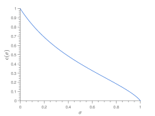
Figure 1: The constant $c(\sigma)$ (re-scaled multiplying by $384$) appearing in Theorem 1.

Discussion.

Given an initial seed $X^{(0)}\in\mathcal{P}_{n}$, the case $N=1$ in Algorithm 2 can be alternatively interpreted as the following two step process: first, compute a similarity matrix $AX^{(0)}B$ and then round the similarity matrix to an actual permutation matrix. This strategy has been frequently applied in graph matching algorithms in both the seeded and seedless case (Umeyama, 1988; Fan et al., 2019; Lubars and Srikant, 2018; Yu et al., 2021b). In terms of the quality of the seed, Theorem 1 gives the same guarantees obtained by (Yu et al., 2021b, Thm.1) which requires $\Omega(\sqrt{n\log n})$ vertices in the seed to be correctly matched. However the results of (Yu et al., 2021b) are specifically for the correlated Erdös-Renyi model.

3.2 Partial recovery in one iteration

In the partial recovery setting, we are interested in the fraction of nodes that are correctly matched. To this end let us define the following measure of performance

$$\operatorname{overlap}(\nu,\nu^{\prime}):=\frac{1}{n}|\{i\in[n]:\nu(i)=\nu^{\prime}(i)\}|$$ (3.2)

for any pair $\nu,\nu^{\prime}\in\mathcal{S}_{n}$. Recall that we assume that the ground truth permutation is $x^{*}=\operatorname{id}$ and $\pi$ is the output of Algorithm 2 with input $(A,B,X^{(0)}=X,N=1)$ where $\Pi=\operatorname{GMWM}(AXB)$. Observe that $\operatorname{overlap}(\pi,x^{*}=\operatorname{id})=s_{\pi}$ is the fraction of fixed points of the permutation $\pi$. It will be useful to consider the following definition. We say that $C_{ij}$ is row-column dominant if $C_{ij}>C_{i^{\prime}j}$ for all $i^{\prime}\neq i$ and $C_{ij}>C_{ij^{\prime}}$, for all $j^{\prime}\neq j$. The following lemma relates the overlap of the output of GMWM with the property that a subset of the entries of $C$ is row-column dominant, its proof is outlined in Appendix C.

Lemma 2.

Let $C$ be a $n\times n$ matrix with the property that there exists a set $\{i_{1},\cdots,i_{r}\}$, with $1\leq r\leq n$ such that $C_{i_{k},i_{k}}$ is row-column dominant for $k\in[r]$. Let $\pi\in\mathcal{S}_{n}$ be permutation corresponding to $\operatorname{GMWM}(C)\in\mathcal{P}_{n}$. Then it holds that $\pi(i_{k})=i_{k}$ for $k\in[r]$ and, in consequence, the following event inclusion holds

$$\{\operatorname{overlap}(\pi,\operatorname{id})<r/n\}\subset\bigcap_{\begin{subarray}{c}I_{r}\subset[n]\\ |I_{r}|=r\end{subarray}}\bigcup_{i\in I_{r}}\{C_{ii}\textup{ is not row-column dominant }\}.$$ (3.3)

Equipped with this lemma, we can prove the following generalization of Theorem 1, its proof is detailed in Section 4.2.

Theorem 2.

Let $A,B\sim W(n,\sigma,\operatorname{id})$ and $X\in\mathcal{P}_{n}$ with $\|X-\operatorname{Id}\|_{F}\leq\theta\sqrt{n}$, where $0\leq\theta\leq\sqrt{2(1-\frac{10}{n})}$ and $n\geq 10$. Let $\pi\in\mathcal{S}_{n}$ be the output of Algorithm 2 with input $(A,B,X^{(0)}=X,N=1)$. Then, for $r\in[n]$

$$\mathbb{P}(\operatorname{overlap}(\pi,\operatorname{id})>r/n)\geq 1-16rne^{-c(\sigma)\big{(}1-\frac{\theta^{2}}{2}\big{)}^{2}n}.$$

In particular, if $x\in\mathcal{S}_{n}$ is the map corresponding to $X$ and $|S_{X}|\geq\sqrt{\frac{1}{c(\sigma)}n\log{(16rn^{2})}}$, then

$$\mathbb{P}(\operatorname{overlap}(\pi,\operatorname{id})>r/n)\geq 1-n^{-1}.$$

3.3 Exact recovery after multiple iterations, uniformly in the seed

The results in Sections 3.1 and 3.2 hold for any given seed $X^{(0)}$, and it is crucial that the seed does not depend on the graphs $A,B$. In this section, we provide uniform convergence guarantees for PPMGM which hold uniformly over all choices of the seed in a neighborhood around $x^{*}$.

Theorem 3.

Let $\sigma\in[0,1)$, $A,B\sim W(n,\sigma,\operatorname{id})$ and define $\kappa:=\left(\frac{9}{410}\right)^{2}(1-\sigma^{2})$. For any $X^{(0)}\in\mathcal{P}_{n}$, denote $X^{(N)}$ the output of PPMGM with input ($\mathcal{H}(A),\mathcal{H}(B),X^{(0)},N=2\log n$), where $\mathcal{H}(M)$ corresponds to the matrix $M$ with the diagonal removed. Then, there exists constants $C^{\prime},c>0$ such that, for all $n\geq\frac{C^{\prime}}{\kappa}\log{n}$, it holds

$$\mathbb{P}\left(\forall X^{(0)}\in\mathcal{P}_{n}\text{ such that }|S_{X^{(0)}}|\geq(1-\kappa)n,X^{(N)}=\operatorname{Id}\right)\geq{\color[rgb]{0,0,0}1-e^{-c\kappa n}-3n^{-2}}.$$

The diagonal of the adjacency matrices $A$ and $B$ in Algorithm 2 was removed in the above theorem only for ease of analysis. Its proof is detailed in Section 4.3. A direct consequence of Theorem 3 is when the seed $X^{(0)}$ is data dependent, i.e., depends on $A,B$. In this case, denoting $\mathcal{E}_{0}=\{|S_{X^{(0)}}|\geq(1-\kappa)n\}$ to be the event that $X^{(0)}$ satisfies the requirement of Theorem 3, and $\mathcal{E}_{unif}$ to be the “uniform” event in Theorem 3, we clearly have by a union bound that

$$\mathbb{P}(X^{(N)}=\operatorname{Id})\geq\mathbb{P}(\mathcal{E}_{0})-\mathbb{P}(\mathcal{E}^{c}_{unif})\geq\mathbb{P}(\mathcal{E}_{0})-e^{-c\kappa n}-3n^{-2}.$$

Hence if $\mathcal{E}_{0}$ holds with high probability, then exact recovery of $X^{*}=\operatorname{Id}$ is guaranteed with high probability as well.

Remark 5.

Contrary to our previous theorems, here the strong consistency of the estimator holds uniformly over all possible seeds that satisfy the condition $|S_{X^{(0)}}|\geq(1-\kappa)n$. For this reason, we need a stronger condition than $|S_{X}|=\Omega(\sqrt{n\log n})$ as was the case in Theorem 1. Our result is non trivial and cannot be obtained from Theorem 1 by taking a union bound. The proof relies on a decoupling technique adapted from (Mao et al., 2021) that used a similar refinement method for CER graphs.

Remark 6.

Contrary to the results obtained in the seedless case that require $\sigma=o(1)$ for exact recovery (Fan et al., 2019), we can allow $\sigma$ to be of constant order. The condition the the fraction of fixed points in the seed be at least $1-\kappa=1-\left(\frac{9}{410}\right)^{2}(1-\sigma^{2})$ seems to be far from optimal as shown in the experiments in Section 5, see Fig. 2. But interestingly, this condition shows that when the noise $\sigma$ increases, PPMGM  needs a more accurate initialization, hence a larger $\kappa$, to recover the latent permutation. This is confirmed by our experiments.

4 Proof outline

4.1 Proof of Theorem 1

For $A,B\sim W(n,\sigma,\operatorname{id})$, the proof of Theorem 1 relies heavily on the concentration properties of the entries of the matrix $C=AXB$, which is the matrix that is projected by our proposed algorithm. In particular, we use the fact that $C$ is diagonally dominant with high probability, under the assumptions of Theorem 1, which is given by the following result. Its proof is delayed to Appendix A.

Proposition 1 (Diagonal dominance property for the matrix $C=AXB$).

Let $A,B\sim W(n,\sigma,\operatorname{id})$ with correlation parameter $\sigma\in[0,1)$ and let $X\in\mathcal{P}_{n}$ with $S_{X}$ the set of its fixed points and $s_{x}:=|S_{X}|/n$. Assume that $s_{x}\geq 10/n$ and that $n\geq 10$. Then the following is true.

1. Noiseless case. For a fixed $i\in[n]$ it holds that

   $$\mathbb{P}\big{(}\exists j\neq i:(AXA)_{ij}>(AXA)_{ii}\big{)}\leq 4ne^{-\frac{s_{x}^{2}}{96}n}.$$

2. For $C=AXB$ and $i\in[n]$ it holds

   $$\mathbb{P}{(\exists j\neq i:C_{ij}>C_{ii})}\leq 5ne^{-c(\sigma)s_{x}^{2}n}$$

   where $c(\sigma)=\frac{1}{384}\frac{1-\sigma^{2}}{1+2\sigma\sqrt{1-\sigma^{2}}}$.

With this we can proceed with the proof of Theorem 1.

Proof of Theorem 1.

To prove part $(i)$ of the theorem it suffices to notice that in Proposition 1 part $(ii)$ we upper bound the probability that $C=AXB$ is not diagonally dominant for each fixed row. Using the union bound, summing over the $n$ rows, we obtain the desired upper bound on the probability that $C$ is not diagonally dominant. We now prove part $(ii)$. Notice that the assumption $\|X-\operatorname{Id}\|_{F}\leq\theta\sqrt{n}$ for $\theta<\sqrt{2}$ implies that $s_{x}$ is strictly positive. Moreover, from this assumption and the fact that $\|X-\operatorname{Id}\|^{2}_{F}=2(n-|S_{X}|)$ we deduce that

$$s_{x}\geq\Big{(}1-\frac{{\theta}^{2}}{2}\Big{)}.$$ (4.1)

On the other hand, we have

$$\mathbb{P}(\Pi\neq\operatorname{Id}) \leq\mathbb{P}(C\text{ is not diag.dom})$$

$$=\mathbb{P}(\exists i,j\in[n],i\neq j:C_{ii}<C_{ij})$$

$$\leq 5n^{2}e^{-c(\sigma)s_{x}^{2}n}$$

$$\leq 5n^{2}e^{-c(\sigma)\big{(}1-\frac{\theta^{2}}{2}\big{)}^{2}n}$$

where we used Lemma 1 in the first inequality, Proposition 1 in the penultimate step and, (4.1) in the last inequality. ∎

4.1.1 Proof of Proposition 1

In Proposition 1 part $(i)$ we assume that $\sigma=0$. The following are the main steps of the proof.

1. We first prove that for all $X\in\mathcal{P}_{n}$ such that $s_{x}=|S_{X}|/n$ and for $i\neq j\in[n]$ the gap $C_{ii}-C_{ij}$ is of order $s_{x}$ in expectation.

2. We prove that $C_{ii}$ and $C_{ij}$ are sufficiently concentrated around its mean. In particular, the probability that $C_{ii}$ is smaller than $s_{x}/2$ is exponentially small. The same is true for the probability that $C_{ij}$ is larger than $s_{x}/2$.

3. We use the fact $\mathbb{P}(C_{ii}\leq C_{ij})<\mathbb{P}(C_{ii}\leq s_{x}/2)+\mathbb{P}(C_{ij}\geq s_{x}/2)$ to control the probability that $C$ is not diagonally dominant.

The proof is mainly based upon the following two lemmas.

Lemma 3.

For the matrix $C=AXA$ and with $s_{x}=|S_{X}|/n$ we have

$$\mathbb{E}[C_{ij}]=\begin{cases}s_{x}+\frac{1}{n}\mathbbm{1}_{i\in S_{X}}\enskip\text{ for }i=j,\\ \frac{1}{n}\mathbbm{1}_{x(j)=i}\enskip\text{ for }i\neq j,\\ \end{cases}$$

and from this we deduce that for $i,j\in[n]$ with $i\neq j$

$$s_{x}-\frac{1}{n}\leq\mathbb{E}{[C_{ii}]}-\mathbb{E}{[C_{ij}]}\leq s_{x}+\frac{1}{n}.$$

Lemma 4.

Assume that $s_{x}\in(10/n,1]$ and $n\geq 10$. Then for $i,j\in[n]$ with $i\neq j$ we have

$$\mathbb{P}(C_{ii}\leq s_{x}/2) \leq 4e^{-\frac{s_{x}^{2}}{48}n},$$ (4.2)

$$\mathbb{P}(C_{ij}\geq s_{x}/2) \leq 3e^{-\frac{s_{x}^{2}}{96}n}.$$ (4.3)

With this we can prove Proposition 1 part $(i)$.

Proof of Prop. 1 $(i)$.

Define the event $\mathcal{E}_{j}=\{C_{ii}<\frac{s_{x}}{2}\}\cup\{C_{ij}>\frac{s_{x}}{2}\}$ and note that for $j\neq i$, we have $\{C_{ij}>C_{ii}\}\subset\mathcal{E}_{j}$. With this and the bounds (4.2) and (4.3) we have

$$\mathbb{P}\big{(}\exists j\neq i:C_{ij}>C_{ii}\big{)} =\mathbb{P}(\cup_{j\neq i}\{C_{ij}>C_{ii}\})$$

$$\leq\mathbb{P}(\cup_{j\neq i}\mathcal{E}_{j})$$

$$\leq\mathbb{P}(C_{ii}\leq\frac{s_{x}}{2})+\sum_{j\neq i}\mathbb{P}(C_{ij}\geq\frac{s_{x}}{2})$$

$$\leq 4e^{-\frac{s_{x}^{2}}{96}n}+3(n-1)e^{-\frac{s_{x}^{2}}{96}n}$$

$$\leq 4ne^{-\frac{s_{x}^{2}}{96}n}.$$

∎

The proof of Lemma 3 is short and we include it in the main body of the paper. On the other hand, the proof of Lemma 4 mainly uses concentration inequalities for Gaussian quadratic forms, but the details are quite technical. Hence we delay its proof to Appendix A.1. Before proceeding with the proof of Lemma 3, observe that the following decomposition holds for the matrix $C$.

$$C_{ij}=\sum_{k,k^{\prime}}A_{ik}X_{k,k^{\prime}}A_{k^{\prime}i}=\begin{cases}\sum_{k\in S_{X}}A^{2}_{ik}+\sum_{k\notin S_{X}}A_{ik}A_{ix(k)}\enskip\text{ for }i=j,\\ \sum^{n}_{k=1}A_{ik}A_{x(k)j}\enskip\text{ for }i\neq j.\end{cases}$$ (4.4)

Proof of Lemma 3.

From (4.4) we have that

$$\mathbb{E}[C_{ii}]=\sum_{k\in S_{X}}\mathbb{E}[A^{2}_{ik}]+\sum_{k\notin S_{X}}\mathbb{E}[A^{2}_{ik}]=\frac{|S_{X}|}{n}+\frac{\mathbbm{1}_{i\in S_{X}}}{n}.$$

Similarly, for $j\neq i$ it holds

$$\mathbb{E}[C_{ij}]=\sum^{n}_{k=1}\mathbb{E}[A_{ik}A_{x(k)j}]=\frac{1}{n}\mathbbm{1}_{i,j\notin S_{X},x(j)=i}=\frac{\mathbbm{1}_{x(j)=i}}{n}$$

from which the results follows easily. ∎

The proof of Proposition 1 part $(ii)$ which corresponds to the case $\sigma\neq 0$ uses similar ideas and the details can be found Appendix A.2.

4.2 Proof of Theorem 2

The proof of Theorem 2 will be based on the following lemma, which extends Proposition 1.

Lemma 5.

For a fixed $i\in[n]$, we have

$$\mathbb{P}(C_{ii}\textup{ is not row-column dominant})\leq 16ne^{-c(\sigma)s_{x}^{2}n}.$$

The proof of Lemma 5 is included in Appendix B. We now prove Theorem 2. The main idea is that for a fixed $i\in[n]$, with high probability the term $C_{ii}$ will be the largest term in the $i$-th row and the $i$-th column, and so GMWM will assign $\pi(i)=i$. We will also use the following event inclusion, which is direct from (3.3) in Lemma 2.

$$\{\operatorname{overlap}(\pi,\operatorname{id})<r/n\}\subset\bigcup^{r}_{i=1}\{C_{ii}\text{ is not row-column dominant }\}.$$ (4.5)

Proof of Theorem 2 .

Fix $i\in[n]$. By (4.5) we have that

$$\mathbb{P}(\operatorname{overlap}(\pi,\operatorname{id})\leq r/n) \leq\sum^{r}_{i=1}\mathbb{P}(C_{ii}\text{ is not row-column dominant})$$

$$\leq\sum^{r}_{i=1}\mathbb{P}(\exists j\neq i,\text{ s.t }C_{ij}\vee C_{ji}>C_{ii})$$

$$\leq 16rne^{-c(\sigma)s_{x}^{2}n}$$

where we used Lemma 5 in the last inequality. ∎

Remark 7.

Notice that the RHS of (4.5) is a superset of the RHS of (3.3). To improve this, it is necessary to include dependency information. In other words, we need to ‘beat Hölder’s inequality’. To see this, define

$$E_{i}:=\mathbbm{1}_{C_{ii}\text{ is not row-column dominant }},\enskip\varepsilon_{I}:=\mathbbm{1}_{\sum_{i\in I}E_{i}>0},\text{ for }I\subset[n];$$

then $\varepsilon_{I^{\prime}}$, for $I^{\prime}=[r]$, is the indicator of the event in the RHS of (4.5). On other hand, the indicator of the event in the RHS of (3.3) is ${\displaystyle\prod_{\begin{subarray}{c}I\subset[n],|I|=r\end{subarray}}}\varepsilon_{I}$. If $\mathbb{E}\big{[}\varepsilon_{I}\big{]}$ is equal for all $I$, then Hölder inequality gives

$$\mathbb{E}\Big{[}{\displaystyle\prod_{\begin{subarray}{c}I\subset[n],|I|=r\end{subarray}}}\varepsilon_{I}\Big{]}\leq\mathbb{E}[\varepsilon_{I^{\prime}}]$$

which does not help in quantifying the difference between (3.3) and (4.5). This is not surprising as we are not taking into account the dependency between the events $\varepsilon_{I}$ for the different sets $I\subset[n],|I|=r$.

4.3 Proof of Theorem 3

The general proof idea is based on the decoupling strategy used by (Mao et al., 2021) for Erdős-Rényi graphs. To extend their result from binary graphs to weighted graphs, we need to use an appropriate measure of similarity. For $i,i^{\prime}\in[n],W\subset[n]$ and $g\in\mathcal{S}_{n}$, let us define

$$\langle A_{i:},B_{i^{\prime}:}\rangle_{g,W}:=\sum_{j\in W}A_{ig(j)}B_{i^{\prime}j}$$

to be the similarity between $i$ and $i^{\prime}$ restricted to $W$ and measured with a scalar product depending on $g$ (the permutation used to align $A$ and $B$). When $g=\operatorname{id}$ or $W=[n]$ we will drop the corresponding subscript(s). If $A$ and $B$ were binary matrices, we would have the following correspondence

$$\langle A_{i:},B_{i^{\prime}:}\rangle_{g,W}=|g(\mathcal{N}_{A}(i)\cap W)\cap\mathcal{N}_{B}(i^{\prime})|.$$

This last quantity plays an essential role in Proposition 7.5 of (Mao et al., 2021). Here $g(\mathcal{S})$ denotes the image of a set $\mathcal{S}\subseteq[n]$ under permutation $g$. This new measure of similarity has two main implications on the proof techniques. Firstly, one can no longer rely on the fact that $\langle A_{i:},B_{i^{\prime}:}\rangle_{g,W}$ is non-negative. Secondly, we will need different concentration inequalities to handle these quantities.

Step 1.

The algorithm design relies on the fact that if the matrices $A$ and $B$ were correctly aligned then the correlation between $A_{i:}$ and $B_{i:}$ should be large and the correlation between $A_{i:}$ and $B_{i^{\prime}:}$ should be small for all $i\neq i^{\prime}$. The following two Lemmas precisely quantify these correlations when the two matrices are well aligned.

Lemma 6 (Correlation between corresponding nodes).

Let $(A,B)\sim W(n,\sigma,x^{*}=\operatorname{id})$ and assume that the diagonals of $A$ and $B$ have been removed. Then for $n$ large enough (larger than a constant), we have with probability at least $1-n^{-2}$ that

$$\langle A_{i:},B_{i:}\rangle\geq\sqrt{1-\sigma^{2}}(1-\epsilon_{1})-\sigma\epsilon_{2}\text{ for all }i\in[n],$$

where $0<\epsilon_{1},\epsilon_{2}\leq C\sqrt{\frac{\log n}{n}}$ for a constant $C>0$.

Lemma 7 (Correlation between different nodes).

Let $(A,B)\sim W(n,\sigma,\operatorname{id})$ and assume that the diagonals of $A$ and $B$ have been removed. Then for $n$ large enough (larger than a constant), we have with probability at least $1-n^{-2}$ that

$$\left|\langle A_{i:},B_{i^{\prime}:}\rangle\right|\leq\sqrt{1-\sigma^{2}}{\color[rgb]{0,0,0}\epsilon_{3}}+\sigma{\color[rgb]{0,0,0}\epsilon_{4}}\text{ for all }i,i^{\prime}\in[n]\text{ such that }i^{\prime}\neq i,$$

where $0<\epsilon_{3},\epsilon_{4}\leq C\sqrt{\frac{\log n}{n}}$ for a constant $C>0$.

The proofs of Lemma’s 6 and 7 can be found in Appendix D.2.

Step 2.

Since the ground truth alignment between $A$ and $B$ is unknown, we need to use an approximate alignment (provided by $X^{(0)}$). It will suffice that $X^{(0)}$ is close enough to the ground truth permutation. This is linked to the fact that if $|S_{X^{(0)}}|$ is large enough then the number of nodes for which there is a substantial amount of information contained in $S_{X^{(0)}}^{c}$ is small. This is shown in the following lemma.

Lemma 8 (Growing a subset of vertices).

Let $G$ a graph generated from the Gaussian Wigner model with self-loops removed, associated with an adjacency matrix $A$. For any $I\subseteq[n]$ and $\kappa\in(0,\frac{1}{2})$, define the random set

$$\tilde{I}=\{i\in[n]:\left\|{A_{i:}}\right\|_{I^{c}}^{2}<8\kappa\}.$$

Then for $n\geq\frac{C^{\prime}}{\kappa}\log{n}$ where $C^{\prime}>0$ is a large enough constant, we have

$$\mathbb{P}\left({\color[rgb]{0,0,0}\forall I\subseteq[n]\text{ with }|I|\geq(1-\kappa)n,\text{ it holds }}|\tilde{I}^{c}|\leq\frac{1}{4}|I^{c}|\right)\geq 1-e^{-c^{\prime}\kappa n}$$

for some constant $c^{\prime}>0$.

In order to prove this lemma we will need the following decoupling lemma.

Lemma 9 (An elementary decoupling).

Let $M>0$ be a parameter and $G$ be a weighted graph on $[n]$, with weights of magnitude bounded by $1$ and without self loops, represented by an adjacency matrix $A\in[-1,1]^{n\times n}$. Assume that there are two subsets of vertices $Q,W\subset[n]$ such that

$$\left\|{A_{i:}}\right\|_{W}^{2}\geq M\text{ for all }i\in Q.$$

Then there are subsets $Q^{\prime}\subseteq Q$ and $W^{\prime}\subseteq W$ such that $Q^{\prime}\cap W^{\prime}=\emptyset$, $|Q^{\prime}|\geq|Q|/5$ and

$$\left\|{A_{i:}}\right\|_{W^{\prime}}^{2}\geq M/2\text{ for all }i\in Q^{\prime}.$$

Proof.

If $|Q\setminus W|\geq|Q|/5$ then one can take $Q^{\prime}=Q\setminus W$ and $W^{\prime}=W$. So we can assume that $|Q\cap W|\geq 4|Q|/5$. Let $\tilde{W}:=W\setminus Q$ and $\hat{Q}$ be a random subset of $Q\cap W$ where each element $j\in Q\cap W$ is selected independently with probability $1/2$ in $\hat{Q}$. Consider the random disjoint sets $\hat{Q}$ and $W^{\prime}:=\tilde{W}\cup((Q\cap W)\setminus\hat{Q})$. First, we will show the following claim.

Claim 1.

For every $i\in Q\cap W$, we have $\mathbb{P}(\left\|{A_{i:}}\right\|_{W^{\prime}}^{2}\geq M/2|i\in\hat{Q})\geq 1/2.$

Indeed, we have by definition

$$\left\|{A_{i:}}\right\|_{W^{\prime}}^{2}=\sum_{j\in W^{\prime}}A_{ij}^{2}=\sum_{j\in W\cap Q}A_{ij}^{2}\mathbf{1}_{j\not\in\hat{Q}}+\sum_{j\in\tilde{W}}A_{ij}^{2}.$$

By taking the expectation conditional on $i\in\hat{Q}$, we obtain

$$\mathbb{E}\left(\left\|{A_{i:}}\right\|_{W^{\prime}}^{2}\middle|i\in\hat{Q}\right)=\sum_{j\in W\cap Q}\frac{A_{ij}^{2}}{2}+\sum_{j\in\tilde{W}}A_{ij}^{2}\geq\frac{1}{2}\sum_{j\in W}A_{ij}^{2}\geq\frac{M}{2}.$$

But since $\sum_{j\in W\cap Q}A_{ij}^{2}(\mathbf{1}_{j\not\in\hat{Q}}-\frac{1}{2})$ is a symmetric random variable we have that

$$\mathbb{P}\left(\left\|{A_{i:}}\right\|_{W^{\prime}}^{2}\geq\mathbb{E}(\left\|{A_{i:}}\right\|_{W^{\prime}}^{2})\middle|i\in\hat{Q}\right)=1/2$$

and hence

$$\mathbb{P}\left(\left\|{A_{i:}}\right\|_{W^{\prime}}^{2}\geq\frac{M}{2}\middle|i\in\hat{Q}\right)\geq 1/2.$$

Consequently, we have

$$\mathbb{E}\left(\sum_{i\in Q\cap W}\mathbf{1}_{\{\left\|{A_{i:}}\right\|_{W^{\prime}}^{2}\geq M/2\}}\mathbf{1}_{i\in\hat{Q}}\right)=\sum_{i\in Q\cap W}\mathbb{P}(i\in\hat{Q})\mathbb{E}\left(\mathbf{1}_{\{\left\|{A_{i:}}\right\|_{W^{\prime}}^{2}\geq M/2\}}\middle|i\in\hat{Q}\right)\geq\frac{|Q\cap W|}{4}\geq\frac{|Q|}{5}.$$

Therefore, there is a realization $Q^{\prime}$ of $\hat{Q}$ such that $Q^{\prime}$ and $W^{\prime}$ satisfy the required conditions. ∎

Proof of Lemma 8.

Let us define $\delta:=8\kappa$, which will be used throughtout this proof. By considering sets $W=I^{c}$ and $Q\subseteq\tilde{I}^{c}$ we obtain the following inclusion

$$\{ {\color[rgb]{0,0,0}\exists I\subseteq[n]\text{ with }|I|\geq(1-\kappa)n,\text{ such that }}|\tilde{I}^{c}|>\frac{1}{4}|I^{c}|\}\subset$$

$$\mathcal{E}:=\{\exists\,Q,W\subseteq[n]:|W|\leq\kappa n,|Q|\geq|W|/4\neq 0,\left\|{A_{i:}}\right\|_{W}^{2}\geq\delta\text{ for all }i\in Q\}.$$

According to Lemma 9, $\mathcal{E}$ is contained in

$$\mathcal{E}^{\prime}:=\{\exists\,Q^{\prime},W^{\prime}\subseteq[n]:|W^{\prime}|\leq\kappa n,|Q^{\prime}|\geq|W|/20\neq 0,Q^{\prime}\cap W^{\prime}=\emptyset,\left\|{A_{i:}}\right\|_{W^{\prime}}^{2}\geq\delta/2\text{ for all }i\in Q^{\prime}\}.$$

For given subsets $Q^{\prime}$ and $W^{\prime}$, the random variables $(\left\|{A_{i:}}\right\|_{W^{\prime}}^{2})_{i\in Q^{\prime}}$ are independent. So, by a union bound argument we get

$$\mathbb{P}\left({\color[rgb]{0,0,0}\exists I\subseteq[n]\text{ with }|I|\geq(1-\kappa)n,\text{ such that }}|\tilde{I}^{c}|>\frac{1}{4}|I^{c}|\right) \leq$$

$$\sum_{w=1}^{\lceil{\kappa n}\rceil}\sum_{|W^{\prime}|=w}\sum_{k=\lceil{w/20}\rceil}^{n}\binom{n}{k} \mathbb{P}\left(\left\|{A_{i:}}\right\|_{W^{\prime}}^{2}\geq\delta/2\right)^{k}.$$

According to Lemma 13, for the choice $t=\kappa n$ we have for all $W^{\prime}$

$$\mathbb{P}\left(\left\|{A_{i:}}\right\|_{W^{\prime}}^{2}\geq\delta/2\right)\leq\mathbb{P}\left(n\left\|{A_{i:}}\right\|_{W^{\prime}}^{2}\geq|W|+\sqrt{|W|t}+2t\right)\leq e^{-\kappa n}.$$

Consequently, for $n$ large enough, we have

$$\mathbb{P}\left({\color[rgb]{0,0,0}\exists I\subseteq[n]\text{ with }|I|\geq(1-\kappa)n,\text{ such that }}|\tilde{I}^{c}|>\frac{1}{4}|I^{c}|\right) \leq$$

$$\sum_{w=1}^{\lceil{\kappa n}\rceil}\sum_{k=\lceil{w/20}\rceil}^{n} \left(\frac{en}{w}\right)^{w}\left(\frac{en}{k}\right)^{k}e^{-k\kappa n}<e^{-c\kappa n},$$

for a constant $c>0$. Indeed, since

$$\frac{en}{ke^{\kappa n}}<1$$

because by assumption $n\geq\frac{C^{\prime}}{\kappa}\log{n}$ , we obtain

$$\sum_{k=\lceil{w/20}\rceil}^{n}\left(\frac{en}{k}\right)^{k}e^{-k\kappa n}\leq C\left(\frac{en}{e^{\kappa n}}\right)^{\lceil{w/20}\rceil}$$

by the property of geometric series, where $C>0$ is a constant. But by the same argument

$$\sum_{w=1}^{\lceil{\kappa n}\rceil}\left(\frac{en}{w}\right)^{w}\left(\frac{(en)^{1/20}}{e^{\kappa n/20}}\right)^{w}\leq\frac{(en)^{1/20}}{e^{\kappa n/20}}\leq e^{-c\kappa n}$$

where $c>0$ is a constant. ∎

Step 3.

We are now in position to show that at each step the set of fixed points of the permutation obtained with PPMGM  increases.

Lemma 10 (Improving a partial matching).

Let $(A,B)\sim W(n,\sigma,\operatorname{id})$ with $\sigma\in[0,1)$, and define

$$\kappa:=\left(\frac{9}{410}\right)^{2}(1-\sigma^{2}).$$

For any $g\in\mathcal{S}_{n}$, let us denote $\tilde{g}$ as the output of one iteration of PPMGM  with $g$ as an input. Then, there exist constants $C^{\prime},c>0$, such that the following is true. If $\frac{n}{\log{n}}\geq\frac{C^{\prime}}{\kappa}$, then with probability at least $1-e^{-c\kappa n}-3n^{-2}$, it holds for all $g\in\mathcal{S}_{n}$ satisfying $|i\in[n]:g(i)=i|\geq(1-\kappa)n$ that

$$|\{i\in[n]:\tilde{g}(i)=i\}|\geq\frac{n}{2}+\frac{|\{i\in[n]:g(i)=i\}|}{2}.$$

Proof.

For any $I\subseteq[n]$ such that $|I|\geq(1-\kappa)n$, define

$$\tilde{I}:= \{i\in[n]:\left\|{A_{i:}}\right\|_{I^{c}}^{2}<8\kappa\},$$

$$\tilde{I}^{\prime}:= \{i\in[n]:\left\|{B_{i:}}\right\|_{I^{c}}^{2}<8\kappa\}.$$

Consider the events

$$\mathcal{E}_{1}^{\prime} :=\{\forall I\subseteq[n]\text{ s.t. }|I|\geq(1-\kappa)n,\text{ it holds that }|\tilde{I}^{c}|\vee|(\tilde{I}^{\prime})^{c}|\leq\frac{1}{4}|I^{c}|\},$$

$$\mathcal{E}_{2}^{\prime} :=\{\forall i\in[n]:\ \langle A_{i:},B_{i:}\rangle\geq 0.9\sqrt{1-\sigma^{2}}\},$$

$$\mathcal{E}_{3}^{\prime} :=\{\forall i\neq i^{\prime}\in[n]:\ |\langle A_{i:},B_{i^{\prime}:}\rangle|<C\sqrt{\log n/n}\},$$

$$\mathcal{E}_{4}^{\prime} :=\{\forall i\in[n]:\ \left\|{A_{i:}}\right\|,\left\|{B_{i:}}\right\|<2\},$$

where $C$ is the constant appearing in Lemmas 6 and 7. Define $\mathcal{E}^{\prime}=\cap_{i=1}^{4}\mathcal{E}_{i}^{\prime}$. By Lemmas 8, 6, 7 and 13 we have

$$\mathbb{P}(\mathcal{E}^{\prime})\geq 1-e^{-c\kappa n}-3n^{-2}.$$

Now condition on $\mathcal{E}^{\prime}$ and take any $g\in\mathcal{S}_{n}$ such that $|\{i\in[n]:g(i)=i\}|\geq(1-\kappa)n$. Define $I$ as the set of fixed points of $g$. For all $i\in\tilde{I}\cap\tilde{I}^{\prime}$ the following holds.

1. We have

   $$\langle A_{i:},B_{i:}\rangle_{g} \geq\langle A_{i:},B_{i:}\rangle-|\langle A_{i:},B_{i:}\rangle_{g,I^{c}}|-|\langle A_{i:},B_{i:}\rangle_{I^{c}}|$$

   $$\geq 0.9\sqrt{1-\sigma^{2}}-2\left\|{A_{i:}}\right\|_{I^{c}}\left\|{B_{i^{\prime}:}}\right\|_{I^{c}} \mathcal{E}^{\prime}_{3} g(I^{c})=I^{c}$$ (by , Cauchy-Schwartz and the fact that )

   $$\geq 0.9\sqrt{1-\sigma^{2}}-16\kappa$$

2. For all $i^{\prime}\neq i$

   $$\langle A_{i:},B_{i^{\prime}:}\rangle_{g} \leq|\langle A_{i:},B_{i^{\prime}:}\rangle|+|\langle A_{i:},B_{i^{\prime}:}\rangle_{I^{c}}|+|\langle A_{i:},B_{i^{\prime}:}\rangle_{g,I^{c}}|$$

   $$\leq C\sqrt{\frac{\log n}{n}}+2\left\|{A_{i:}}\right\|_{I^{c}}\left\|{B_{i^{\prime}:}}\right\|_{I^{c}} \mathcal{E}^{\prime}_{3} g(I^{c})=I^{c}$$ (by , Cauchy-Schwartz and the fact that )

   $$\leq C\sqrt{\frac{\log n}{n}}+12\sqrt{\kappa}$$

   since $i\in\tilde{I}\cap\tilde{I}^{\prime}$ and $\left\|{B_{i^{\prime}:}}\right\|_{I^{c}}\leq\left\|{B_{i^{\prime}:}}\right\|\leq 2$ on the event $\mathcal{E}_{4}^{\prime}$.

3. Arguing in the same way, we have for all $i^{\prime}\neq i$

   $$\langle A_{i^{\prime}:},B_{i:}\rangle_{g}\leq C\sqrt{\frac{\log n}{n}}+12\sqrt{\kappa}.$$

Since the condition on $n$ implies $C\sqrt{\frac{\log n}{n}}\leq 12\sqrt{\kappa}$, and $\kappa\in(0,1)$, it follows that for all $i\in\tilde{I}\cap\tilde{I}^{\prime}$ and $i^{\prime}\neq i$

$$\langle A_{i:},B_{i:}\rangle_{g} \geq 0.9\sqrt{1-\sigma^{2}}-16\sqrt{\kappa},$$

$$\langle A_{i:},B_{i^{\prime}:}\rangle_{g}\vee\langle A_{i^{\prime}:},B_{i:}\rangle_{g} \leq 25\sqrt{\kappa}.$$

Thus, from the stated choice of $\kappa$, we have for all $i\in\tilde{I}\cap\tilde{I}^{\prime}$ and $i^{\prime}\neq i$ that

$$\langle A_{i:},B_{i:}\rangle_{g}\geq\langle A_{i:},B_{i^{\prime}:}\rangle_{g}\vee\langle A_{i^{\prime}:},B_{i:}\rangle_{g}.$$

In particular, this implies that for all $i\in\tilde{I}\cap\tilde{I}^{\prime}$, $(AGB)_{ii}$ is row-column dominant, where $G\in\mathcal{P}_{n}$ corresponds to $g\in\mathcal{S}_{n}$. Hence, $\tilde{g}$ (the output of PPMGM) will correctly match $i$ with itself. Then clearly $\tilde{g}$ will be such that

$$|\{i\in[n]:\tilde{g}(i)=i\}| \geq|\tilde{I}\cap\tilde{I}^{\prime}|$$ (by inclusion)

$$\geq n-|\tilde{I}^{c}|-|(\tilde{I}^{\prime})^{c}|$$ (by union bound)

$$\geq\frac{n}{2}+\frac{|\{i\in[n]:g(i)=i\}|}{2}. \mathcal{E}^{\prime}_{1}$$ (by )

∎

Conclusion.

By Lemma 10, if the initial number of fixed points is $(1-\kappa)n$ then after one iteration step the size of the set of fixed points of the new iteration is at least $(1-\kappa/2)n$ with probability greater than $1-e^{-c\kappa n}-3n^{-2}$. So after $2\log n$ iterations the set of fixed points has size at least $(1-\kappa/2^{2\log n})n>n-1$ with probability greater than $1-e^{-c\kappa n}-3n^{-2}$. Note that the high probability comes from the conditioning on the event $\mathcal{E}^{\prime}$ so it is not necessary to take a union bound for each iteration.

5 Numerical experiments

In this section, we present numerical experiments to assess the performance of the PPMGM algorithm and compare it to the state-of-art algorithms for graph matching, under the CGW model. We divide this section in two parts. In Section 5.1 we generate CGW graphs $A,B\sim W(n,\sigma,x^{*})$ for a random permutation $x^{*}$, and apply to $A,B$ the spectral algorithms Grampa (Fan et al., 2019), the classic Umeyama (Umeyama, 1988), and the convex relaxation algorithm QPADMM, which first solves the following convex quadratic programming problem

$$\max_{X\in\mathcal{B}_{n}}\|AX-XB\|^{2}_{F},$$ (5.1)

where $\mathcal{B}_{n}$ is the Birkhoff polytope of doubly stochastic matrices, and then rounds the solution using the greedy method GMWM. All of the previous algorithms work in the seedless case. As a second step, we apply algorithm PPMGM with the initialization given by the output of Grampa, Umeyama and QPADMM. We show experimentally that by applying PPMGM the solution obtained in both cases improves, when measured as the overlap (defined in (3.2)) of the output with the ground truth. We also run experiments by initializing PPMGM with $X^{(0)}$ randomly chosen at a certain distance of the ground truth permutation $X^{*}$. Specifically, we select $X^{(0)}$ uniformly at random from the set of permutation matrices that satisfy $\|X^{(0)}-X^{*}\|_{F}=\theta^{\prime}\sqrt{n}$, and vary the value of $\theta^{\prime}\in[0,\sqrt{2})$.

In Section 5.2 we run algorithm PPMGM with different pairs of input matrices. We consider the Wigner correlated matrices $A,B$ and also the pairs of matrices ($A^{\operatorname{spar}_{1}},B^{\operatorname{spar}_{1}}$), ($A^{\operatorname{spar}_{2}},B^{\operatorname{spar}_{2}}$) and ($A^{\operatorname{spar}_{3}},B^{\operatorname{spar}_{3}}$), which are produced from $A,B$ by means of a sparsification procedure (detailed in Section 5.2). The main idea behind this setting is that, to the best of our knowledge, the best theoretical guarantees for exact graph matching have been obtained in (Mao et al., 2021) for relatively sparse Erdős-Rényi graphs. The algorithm proposed in (Mao et al., 2021) has two steps, the first of which is a seedless type algorithm which produces a partially correct matching, that is later refined with a second algorithm (Mao et al., 2021, Alg.4). Their proposed algorithm RefinedMatching shares similarities with PPMGM and with algorithms 1-hop (Lubars and Srikant, 2018; Yu et al., 2021b) and 2-hop (Yu et al., 2021b). Formulated as it is, RefinedMatching (Mao et al., 2021) (and the same is true for 2-hop for that matter) only accepts binary edge graphs as input and also uses a threshold-based rounding approach instead of Algorithm 1, which might be difficult to calibrate in practice. With this we address experimentally the fact that the analysis (and algorithms) in (Mao et al., 2021) does not extend automatically to a simple ‘binarization’ of the (dense) Wigner matrices, and that specially in high noise regimes, the sparsification strategies do not perform very well.

5.1 Performance of PPMGM

In Figure 2(a) we plot the recovery fraction, which is defined as the overlap (see (3.2)) between the ground truth permutation and the output of five algorithms: Grampa, Umeyama, Grampa+PPMGM, Umeyama+PPMGM and PPMGM. The algorithms Grampa+PPMGM and Umeyama+PPMGM use the output of Grampa and Umeyama as seeds for PPMGM, which is performed with $N=1$. In the algorithm PPMGM, we use an initial permutation $x^{(0)}\in\mathcal{S}_{n}$ chosen uniformly at random in the set of permutations such that $\operatorname{overlap}{(x^{(0)},x^{*})}=0.1$; this is referred to as ‘PPMGM rand.init’. We take $n=800$ and plot the average overlap over $25$ Monte Carlo runs. The area comprises $90\%$ of the Monte Carlo runs (leaving out the $5\%$ smaller and the $5\%$ larger). As we can see from this figure, the performance of PPMGM initialized with a permutation with $0.1$ overlap with the ground truth outperforms Grampa and Umeyama (and also their refined versions, where PPMGM is used as a post-processing step). Overall, the PPMGM improves the performance of those algorithms, provided that their output has a reasonably good recovery. From Fig.2(a), we see that Grampa and Umeyame fail to provide a permutation with good overlap with the ground truth for larger values of $\sigma$ (for example, at $\sigma=0.5$ both algorithms have a recovery fraction smaller than $0.1$). In Figure 2(b) we plot the performance of the PPMGM algorithm for randomly chosen seeds and with different number of correctly pre-matched vertices. More specifically, we consider an initial permutation $x^{(0)}_{j}\in\mathcal{S}_{n}$ (corresponding to initializations $X^{(0)}_{j}\in\mathcal{P}_{n}$) for $j=1,\cdots,6$ with $\operatorname{overlap}(x^{(0)}_{1},x^{*})=0.04$, $\operatorname{overlap}(x^{(0)}_{2},x^{*})=0.0425$, $\operatorname{overlap}(x^{(0)}_{3},x^{*})=0.{045}$, $\operatorname{overlap}(x^{(0)}_{4},x^{*})=0.05$, $\operatorname{overlap}(x^{(0)}_{5},x^{*})=0.06$ and $\operatorname{overlap}(x^{(0)}_{6},x^{*})=0.1$. Equivalently, we have $\|X^{(0)}_{j}-X^{*}\|_{F}=\theta^{\prime}_{j}\sqrt{n}$, where $\theta^{\prime}_{j}=\sqrt{2\big{(}1-\operatorname{overlap}(x^{(0)}_{j},x^{*})\big{)}}$. Each permutation $x^{(0)}_{j}$ is chosen uniformly at random in the subset of permutations that satisfy each overlap condition. We observe that initializing the algorithm with an overlap of $0.1$ with the ground truth permutation already produces perfect recovery in one iteration for levels of noise as high as $\sigma=0.8$. Interestingly, the variance over the Monte Carlo runs diminishes as the overlap with the ground truth increases. In Fig.2(b) the shaded area contains $90\%$ of the Monte Carlo runs for the case of $in.4$, $in.5$ and $in.6$ (given the very high variance of the Monte Carlo for the rest, we opt not to share their $90\%$ area for readability purposes).

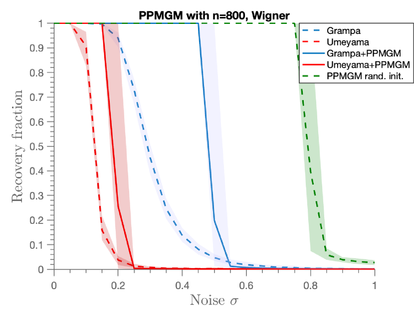
(a) Performance of PPMGM as a refinement of Grampa and Umeyama algorithms, compared with PPM with a random initialization $x^{(0)}$, such that $\operatorname{overlap}(x^{(0)},x^{*})=0.1$. The lines represent the average fraction of recovery over $25$ Monte Carlo runs. The shaded area contains $90\%$ of the Monte Carlo runs.

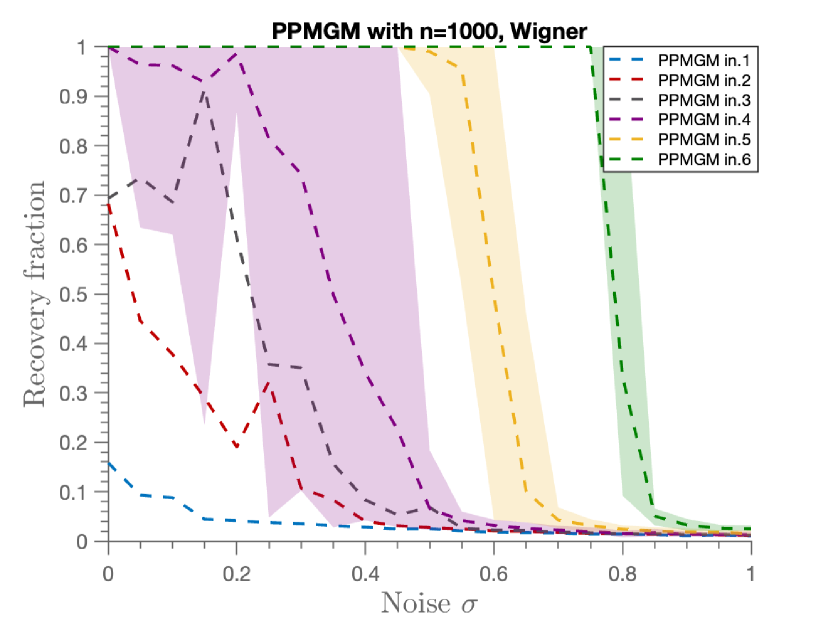
(b) Performance of PPMGM with different initializations. Here $in.1,in.2,in.3,in.4,in.5,in.6$ correspond to respective overlaps of $0.04,0.0425,0.045,0.05,0.06$,$0.1$ of $x^{(0)}$ with the ground truth. We shade the area with $90\%$ of Monte Carlo runs for $in.4,in.5$ and $in.6$ (for the rest, the variance is too high).

Figure 2: We plot the performance of PPMGM as a refinement (post-processing) method of seedless graph matching algorithms, and with random initializations (uniform on different Frobenius spheres ).

In Figure 3 we illustrate the performance of PPMGM, when is used as a refinement of the seedless algorithm QPADMM, which solves (5.1) via the alternating direction method of multipliers (ADMM). This setting has also been considered in the numerical experiments in (Ding et al., 2021; Fan et al., 2019). We plot the average performance over $25$ Monte Carlo runs of the methods QPADMM and QPADMM+PPMGM (its refinement), and we include the performance of Grampa and Grampa+PPMGM for comparison. As before, the shaded area contains $90\%$ of the Monte Carlo runs. It is clear that QPADMM+PPMGM outperforms the rest which is a consequence of the good quality of the seed of QPADMM. The caveat is that QPADMM takes much longer to run than Grampa. In our experiments, for $n=200$, it is $2.5$ times slower on average, although in (Fan et al., 2019) a larger gap is reported for $n=1000$. This shows the scalability issues of QPADMM which is not surprising considering that general purpose convex solvers are usually much slower than first order methods.

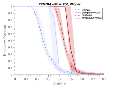
Figure 3: Performance of PPMGM used as a refinement (post-processing) of QPADMM for $n=200$ and $25$ Monte Carlo runs. We include the results of Grampa and its refinement for comparison purposes.

Varying the number of iterations $N$.

We experimentally evaluate the performance of PPMGM when varying the number of iterations $N$ in Algorithm 2. In Figure 4 we plot the recovery rate of PPMGM, initialized with $x^{(0)}$, with an overlap of $0.1$ with the ground truth. In Fig. 4(a) we see that adding more iterations increases the performance of the algorithm for $n=500$; however the improvement is less pronounced in the higher noise regime. In other words, the number of iterations cannot make up for the fact that the initial seed is of poor quality (relative to the noise level). We use $N=1,2,4,8,30$ iterations and we observe a moderate gain between $N=8$ and $N=30$. In Fig. 4(b) we use a matrix of size $n=1000$ and we see that the difference between using $N=1$ and $N>1$ is even less pronounced ( we omit the case of $30$ iterations for readability purposes, as it is very similar to $N=8$). This is in concordance with our main results, as the main quantities used by our algorithm are getting more concentrated as $n$ grows. In the case of one iteration, Proposition 1 says that the probability that the diagonal elements of the gradient term $AXB$ are the largest in their corresponding row is increasing with $n$ (we recall that we can assume that the ground truth is the identity w.l.o.g), which means that the probability of obtaining exact recovery, after the GMWM rounding, is increasing with $n$. This is verified experimentally here (comparing the blue curve in Fig. 4(a) and Fig. 4(b)). An analogous reasoning follows from Lemmas 6 and 7 in the case of multiple iterations. Ultimately, when $n$ increases, the relative performance of PPMGM with $N=1$ increases and there is less room for improvement using more iterations (altough the improvement is still significant).

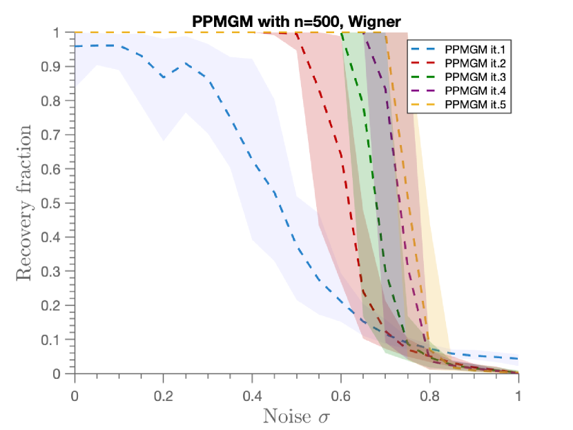
(a) PPMGM with an initialization such that $\operatorname{overlap}(x^{(0)},x^{*})=0.1$. Here $it.1,it.2,it.3,it.4,it.5$ corresponds to $1,2,4,8$ and $30$ iterations respectively.

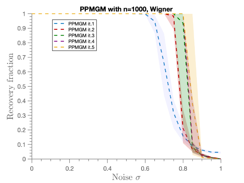
(b) Here $it.1,it.2,it.3,it.4$ corresponds to $1,2,4$ and $8$ iterations respectively.

Figure 4: Comparison of the performance of PPMGM with different values of $N$ (number of iterations).

5.2 Sparsification strategies

Here we run PPMGM using different input matrices which are all transformations of the Wigner correlated matrices $A,B$. Specifically, we compare PPMGM with $A,B$ as input with the application of PPMGM to three different pairs of input matrices ($A^{\operatorname{spar}_{1}},B^{\operatorname{spar}_{1}}$), ($A^{\operatorname{spar}_{2}},B^{\operatorname{spar}_{2}}$) and ($A^{\operatorname{spar}_{3}},B^{\operatorname{spar}_{3}}$) that are defined as follows.

$$A^{\operatorname{spar}_{1}}_{ij} =\mathbbm{1}_{|A_{ij}|<\tau};\enskip B^{\operatorname{spar}_{1}}_{ij}=\mathbbm{1}_{|B_{ij}|<\tau},$$

$$A^{\operatorname{spar}_{2}}_{ij} =A_{ij}\mathbbm{1}_{|A_{ij}|<\tau};\enskip B^{\operatorname{spar}_{2}}_{ij}=B_{ij}\mathbbm{1}_{|B_{ij}|<\tau},$$

$$A^{\operatorname{spar}_{3}}_{ij} =A_{ij}\mathbbm{1}_{|A_{ij}|\in\operatorname{top_{k}}(A_{i:})};\enskip B^{\operatorname{spar}_{2}}_{ij}=B_{ij}\mathbbm{1}_{|B_{ij}|\in\operatorname{top_{k}}(B_{i:})},$$

where $\tau>0$ and for $k\in\mathbb{N}$ and a $n\times n$ matrix $M$, $\operatorname{top_{k}}(M_{i:})$ is the set of the $k$ largest elements (breaking ties arbitrarily) of $M_{i:}$ (the $i$-th row of $M$). The choice of the parameter $\tau$ is mainly determined by the sparsity assumptions in (Mao et al., 2021, Thm.B), i.e., if $G,H$ are two CER graphs to be matched with connection probability $p$ (which is equal to $qs$ in the definition (1.1)), then the assumption is that

$$(1+\epsilon)\frac{\log n}{n}\leq p\leq n^{\frac{1}{R\log\log n}-1}$$ (5.2)

where $\epsilon>0$ is arbitrary and $R$ is an absolute constant. We refer the reader to (Mao et al., 2021) for details. For each $p$ in the range defined by (5.2) we solve the equation

$$\mathbb{P}(|A_{ij}|\leq\tau_{p})=2\Phi(-\tau_{p}\sqrt{n})=p$$ (5.3)

where $\Phi$ is the standard Gaussian cdf (which is bijective so $\tau_{p}$ is well defined). In our experiments, we solve (5.3) numerically. Notice that $A^{\operatorname{spar}_{1}}$ and $B^{\operatorname{spar}_{1}}$ are sparse CER graphs with a correlation that depends on $\sigma$. For the value of $k$ that defines $A^{\operatorname{spar}_{3}},B^{\operatorname{spar}_{3}}$ we choose $k=\Omega(\log n)$ or $k=\Omega(n^{o(1)})$, to maintain the sparsity degree in (5.2). In Figure 5 we plot the performance comparison between the PPMGM without sparsification, and the different sparsification strategies. We see in Figs. 5(a) and 5(b) (initialized with overlap $0.5$ and $0.1$) that the use of the full information $A,B$ outperforms the sparser versions in the higher noise regimes and for small overlap of the initialization. On the other hand, the performance tends to be more similar for low levels of noise and moderately large number of correct initial seeds. In theory, sparsification strategies have a moderate denoising effect (and might considerably speed up computations), but this process seems to destroy important correlation information.

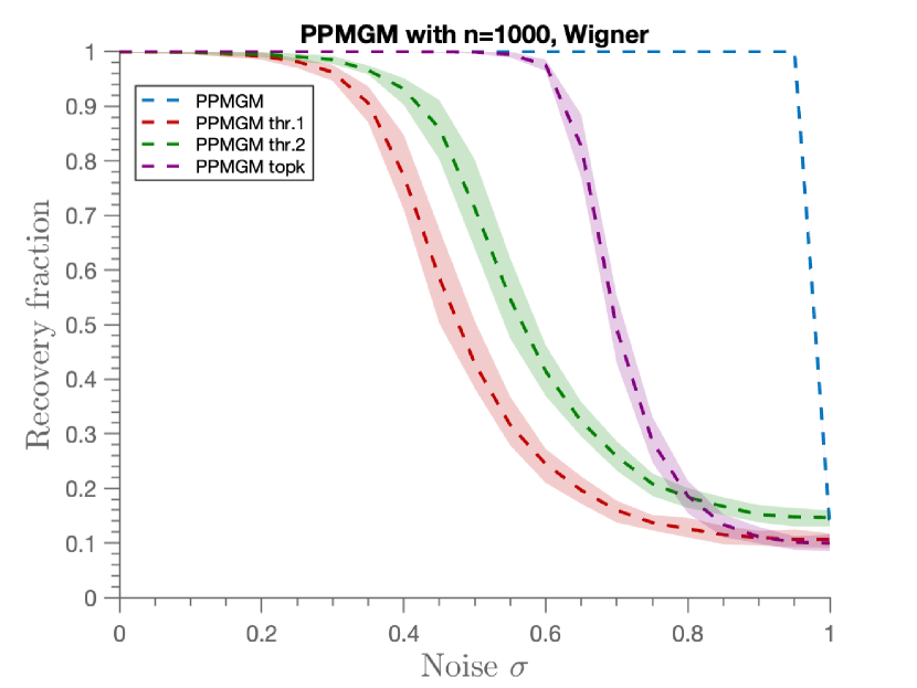
(a) Initial overlap is equal to $0.5$

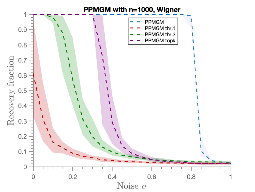
(b) Initial overlap is equal to $0.1$

Figure 5: Comparison between PPMGM with and without sparsification. Here $thr.1$ corresponds to the pair of matrices ($A^{\operatorname{spar}_{1}},B^{\operatorname{spar}_{1}}$), $thr.2$ corresponds to the pair ($A^{\operatorname{spar}_{2}},B^{\operatorname{spar}_{2}}$) and top $k$ corresponds to ($A^{\operatorname{spar}_{3}},B^{\operatorname{spar}_{3}}$)

5.2.1 Choice of the sparsification parameter $\tau$

Solving (5.3) for $p$ in the range (5.2) we obtain a range of possible values for the sparsification parameter $\tau$. To choose between them, we use a simple grid search where we evaluate the recovery rate for each sparsification parameter on graphs of size $n=1000$, and take the mean over $25$ independent Monte Carlo runs. In Fig. 6, we plot a heatmap with the results. We see that the best performing parameter in this experiment was for $\tau_{5}$ corresponding to a probability $p_{5}=51\times 10^{-3}$, although there is a moderate change between all the choices for $p$.

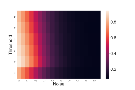
Figure 6: Heatmap for the recovery rate of PPMGM algorithm with input ($A^{\operatorname{spar}_{1}},B^{\operatorname{spar}_{1}}$) for different threshold values $\tau_{i}$($y$ axis); $i=1,\cdots,6$, and different values of $\sigma$ ($x$ axis). Here $\tau_{i}$ corresponds to the solution of (5.3) with $n=1000$ and $p_{i}$ for $i=1,2\cdots,6$ in a uniform grid between $p_{1}=42\times 10^{-3}$ and $p_{6}=54\times 10^{-3}$.

5.3 Real data

We evaluate the performance of PPMGM for the task of matching 3D deformable objects, which is fundamental in the field of computer vision. We use the SHREC’16 dataset (Lähner et al., 2016) which contains $25$ shapes of kids (that can be regarded as perturbations of a single reference shape) in both high and low-resolution, together with the ground truth assignment between different pairs of shapes. Each image is represented by a triangulation (a triangulated mesh graph) which is converted to a weighted graph by standard image processing methods (Peyré, 2008). More specifically, each vertex corresponds to a point in the image (its triangulation) and the edge weights are given by the distance between the vertices. We use the low-resolution dataset in which each image is codified by a graph whose size varies from $8608$ to $11413$ vertices and where the average number of edges is around $0.05\%$ (high degree of sparsity). The main objective in this section is to show experimental evidence that PPMGM improves the quality of a matching given by a seedless algorithm, and for that, the pipeline is as follows.

1. We first make the input graphs of the same size by erasing, uniformly at random, the vertices of the larger graph.

2. We run Grampa algorithm to obtain a matching.

3. We use the output of Grampa as the initial point for PPMGM.

We present an example of the results in Figure 7 where we choose two images and find a matching between them following the above steps. We choose these two images based on the fact that the sizes of the graphs that represent them are the most similar in the whole dataset ($11265$ and $11267$ vertices). We can see visually that the final matching obtained by PPMGM maps mostly similar parts of the body in the two shapes.

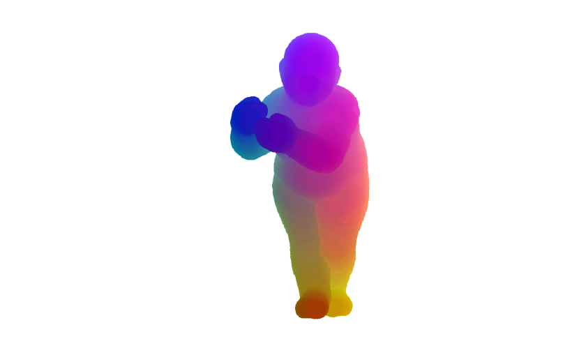
(a)

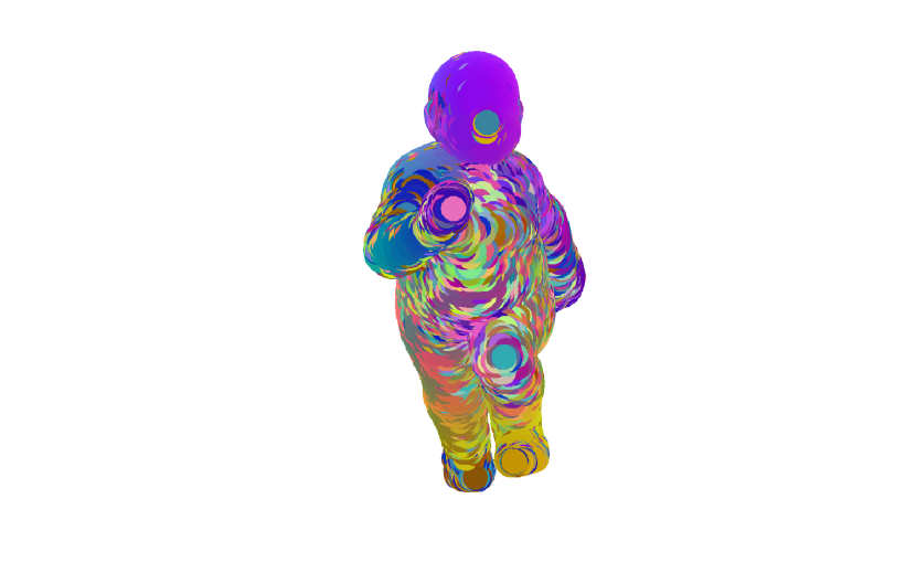
(b)

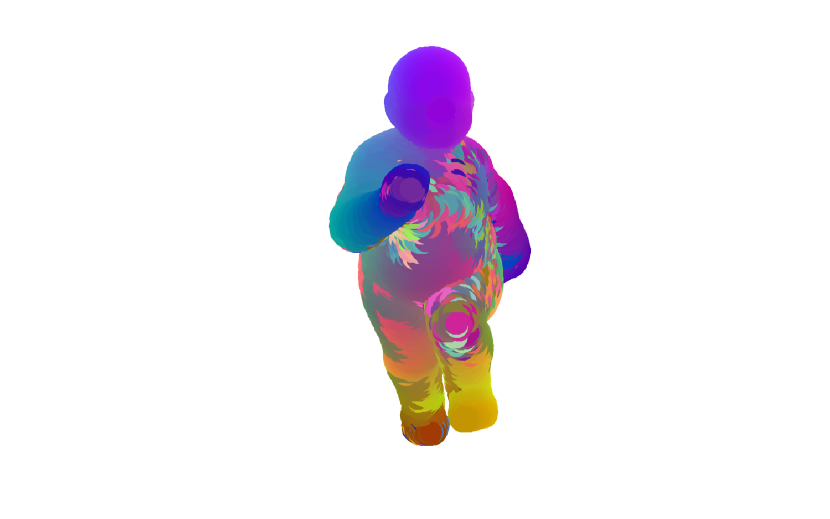
(c)

Figure 7: Visual representation of the performance of PPMGM (with $100$ iterations), improving the results of Grampa algorithm. Fig. 7(a) is the reference shape (graph $A$) where different colours are assigned to different parts of the body. Fig. 7(b) is the second shape (graph $B$) where the colours are assigned according to the matching given by Grampa algorithm; the accuracy is around $27\%$. Fig. 7(c) shows the results of PPMGM, taking as the initial point the output of Grampa in Fig. 7(b). The accuracy is improved to around $57\%$.

Following the experimental setting in (Yu et al., 2021b), we evaluate the performance of PPMGM using the Princeton benchmark protocol (Kim et al., 2011). Here we take all the pairs of shapes in the SHREC’16 dataset and apply the steps $1$ to $3$, of the pipeline described above, to them. Given graphs $A$ and $B$ (corresponding to two different shapes) we compute the normalized geodesic error as follows. For each node $i$ in the shape $A$, we compute $d_{B}(\hat{\pi}_{\operatorname{ppm}}(i),\pi^{*}(i))$, where $\hat{\pi}$ is the output of PPMGM, $\pi^{*}$ is the ground truth matching between $A$ and $B$ and $d_{B}$ is the geodesic distance on $B$ (computed as the weighted shortest path distance using the triangulation representation of the image (Peyré, 2008)). We then define the normalized error as $\varepsilon_{\operatorname{ppm}}(i):=d_{B}(\hat{\pi}_{\operatorname{ppm}}(i),\pi^{*}(i))/\sqrt{\operatorname{Area}(B)}$, where $\operatorname{Area}(B)$ is the surface area of $B$ (again computed using the triangulation representation). Then the cumulative distribution function (CDF) is defined as follows.

$$\operatorname{CDF}_{\operatorname{ppm}}(\epsilon)=\sum^{n_{A}}_{i=1}\mathbbm{1}_{\varepsilon_{\operatorname{ppm}}(i)\leq\epsilon},$$

where $n_{A}$ is the number of nodes of $A$.

In Figure 8 we compare $\operatorname{CDF}_{\operatorname{ppm}}$ with $\operatorname{CDF}_{\operatorname{grampa}}$, which is defined in an analogous way by using $\varepsilon_{\operatorname{grampa}}(i):=d_{B}(\hat{\pi}_{\operatorname{grampa}}(i),\pi^{*}(i))/\sqrt{\operatorname{Area}(B)}$ instead of $\varepsilon_{\operatorname{ppm}}$ (here $\hat{\pi}_{\operatorname{grampa}}$ is output of Grampa). We observe that the performance increases overall for all the values of $\epsilon\in[0,1]$. In particular, the average percentage of nodes correctly matched (corresponding to $\epsilon=0$) increases from less than $15\%$ in the Grampa baseline to more than $50\%$ with PPMGM. Compared to the results in (Yu et al., 2021b), the performance of PPMGM is similar to their $1$-hop algorithm (although here we used the weighted adjacency matrix). The performance of PPMGM is slightly worse than what they reported for the $2$-hop algorithm. Regarding the latter, it is worth noting that, although the iterated application of their $2$-hop algorithm performs well in their experiments, no theoretical guarantees are provided beyond the case of one iteration. It is possible that our analysis can be extended to the case of multiple iterations of the $2-$hop algorithm, but this is beyond the scope of the present paper.

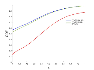
Figure 8: Average performance of PPMGM algorithm, with $N=30$ and $N=100$ iterations, when used to boost the performance of Grampa algorithm. The average is over all pairs of graphs (shapes) of the SHREC’16 database.

6 Concluding remarks

In this work, we analysed the performance of the projected power method (proposed in (Onaran and Villar, 2017)) as a seeded graph matching algorithm, in the correlated Wigner model. We proved that for a non-data dependent seed with $\mathcal{O}(\sqrt{n\log n})$ correctly pre-assigned vertices, the PPM exactly recovers the ground truth matching in one iteration. This is analogous to the state-of-the-art results for algorithms in the case of relatively sparse correlated Erdős-Rényi graphs. We additionally proved that the PPM can exactly recover the optimal matching in $\mathcal{O}(\log n)$ iterations for a seed that contains $\Omega\big{(}(1-\kappa)n\big{)}$ correctly matched vertices, for a constant $\kappa\in(0,1)$, even if the seed can potentially be dependent on the data. For the latter result, we extended the arguments of (Mao et al., 2021) from the (sparse) CER model to the (dense) CGW case, providing a uniform control on the error when the seed contains $\Omega\big{(}(1-\kappa)n\big{)}$ fixed points. This provides theoretical guarantees for the use of PPM as a refinement algorithm (or a post-processing step) for other seedless graph matching methods.

An open question is to find an efficient initialization method which outputs a permutation with order $(1-\kappa)n$ correctly matched vertices in regimes with higher $\sigma$ (say for $\sigma>1/2$). For those noise levels, spectral methods do not seem to perform well (at least in the experiments). An idea could be to adapt the results (Mao et al., 2021) from the sparse CER case to the CGW case. In that paper, the authors construct for each vertex a signature containing the neighborhood information of that vertex and which is encoded as tree. Then a matching is constructed by matching those trees. It is however unclear how to adapt those results (which heavily rely on the sparsity) to the CGW setting.

Appendix A Proof of Proposition 1

We divide the proof into two subsections. In Appendix A.1 we prove Lemma 4 and in Appendix A.2 we prove part $(ii)$ of Proposition 1. Before proceeding, let us introduce and recall some notation. Define $C^{\prime}:=AXA$ and $C^{\prime\prime}:=AXZ$, then $C=AXB=\sqrt{1-\sigma^{2}}C^{\prime}+\sigma C^{\prime\prime}$. Recall that for a permutation $x$, $S_{X}$ will denote the set of fixed points of $x$ (the set of non-zero diagonal terms of its matrix representation $X$) and we will often write $s_{x}=|S_{X}|/n=Tr(X)/n$. We will say that a real random variable $Y\sim\chi^{2}_{K}$ if it follows a central Chi-squared distribution with $K$ degrees of freedom.

A.1 Proof of Lemma 4

The proof of Lemma 4 mainly revolves around the use of concentration inequalities for quadratic forms of Gaussian random vectors. For that, it will be useful to use the following representation of the entries of $C$.

$$C_{ij}=\langle A_{:i},XA_{:j}\rangle$$ (A.1)

where we recall that $A_{:k}$ represents the $k$-th column of the matrix $A$.

Proof of Lemma 4.

High probability bound for $C_{ii}$.

Define $\tilde{a}_{i}$ to be a vector in $\mathbb{R}^{n}$ such that

$$\tilde{a}_{i}(k)=\begin{cases}A_{ki},\text{ for }k\notin{i,x^{-1}(i)},\\ \frac{1}{\sqrt{2}}A_{ii},\text{ for }k\in{i,x^{-1}(i)}.\end{cases}$$

Using representation (A.1) we have

$$C_{ii}=\langle\tilde{a}_{i},X\tilde{a}_{i}\rangle+\mathcal{Z}_{i}$$

where

$$\mathcal{Z}_{i}:=\frac{1}{2}A_{ii}\big{(}A_{x(i)i})+A_{x^{-1}(i)i}\big{)}.$$

It is easy to see that $\sqrt{n}\tilde{a}_{i}$ is a standard Gaussian vector. Using Lemma 14 we obtain

$$n\langle\tilde{a}_{i},X\tilde{a}_{i}\rangle\stackrel{{\scriptstyle d}}{{=}}\sum^{n_{1}}_{i=1}\mu_{i}g^{2}_{i}-\sum^{n_{2}}_{i=1}\nu_{i}g^{\prime 2}_{i}$$

where $(\mu_{i})^{n_{1}}_{i=1},(-\nu_{i})^{n_{2}}_{i=1}$, (with $\mu_{i}\geq 0$, $\nu_{i}\geq 0$ and $n_{1}+n_{2}=n$) is the sequence of eigenvalues of $\frac{1}{2}(X+X^{T})$ and $g=(g_{1},\cdots,g_{n_{1}})$, $g^{\prime}=(g^{\prime}_{1},\cdots,g^{\prime}_{n_{2}})$ are two independent sets of i.i.d standard Gaussians. Lemma 14 tell us in addition that $\|\mu\|_{1}-\|\nu\|_{1}=s_{x}n$, $\|\mu\|_{2}+\|\nu\|_{2}\leq\sqrt{2n}$ and $\|\mu\|_{\infty},\|\nu\|_{\infty}\leq 1$. Using Corollary 1 (D.2), we obtain

$$\mathbb{P}(n\langle\tilde{a}_{i},X\tilde{a}_{i}\rangle\leq s_{x}n-2\sqrt{2nt}-2t)\leq e^{-t}$$ (A.2)

for all $t\geq 0$. To obtain a concentration bound for $\mathcal{Z}_{i}$ we will distinguish two cases.

(a)Case $i\in S_{X}$. In this case, we have $\mathcal{Z}_{i}=a^{2}_{i}(i)$, which implies that $C_{ii}\geq\langle\tilde{a}_{i},X\tilde{a}_{i}\rangle$. Hence

$$\mathbb{P}(nC_{ii}\leq s_{x}n-2\sqrt{2nt}-2t)\leq 2e^{-t}.$$

Replacing $t=\overline{t}:=\frac{n}{2}(\sqrt{1+\frac{s_{x}}{2}}-1)^{2}$ in the previous expression, one can verify that $\overline{t}\geq\frac{n}{48}s_{x}^{2}$, for $s_{x}\in(0,1]$, hence

$$\mathbb{P}(C_{ii}\leq s_{x}/2)\leq 2e^{-\frac{s_{x}^{2}}{48}n}$$

which proves (4.2) in this case.

(b) Case $i\notin S_{X}$. Notice that in this case, $a_{i}(i)$ is independent from $(a_{i}(x(i))+a_{i}(x^{-1}(i))$, hence $n\mathcal{Z}_{i}\stackrel{{\scriptstyle d}}{{=}}g_{1}g_{2}$, where $g_{1},g_{2}$ are independent standard Gaussians. Using the polarization identity $g_{1}g_{2}=\frac{1}{4}(g_{1}+g_{2})^{2}-\frac{1}{4}(g_{1}-g_{2})^{2}$, we obtain

$$n\mathcal{Z}_{i}\stackrel{{\scriptstyle d}}{{=}}\frac{1}{2}(\tilde{g}^{2}_{1}-\tilde{g}^{2}_{2})$$

where $\tilde{g_{1}},\tilde{g_{2}}$ are independent standard Gaussians. By Corollary 1 we have

$$\mathbb{P}\Big{(}2n\mathcal{Z}_{i}\leq-4\sqrt{t}-2t\Big{)}\leq 2e^{-t}.$$ (A.3)

Using (A.2) and (A.3), we get

$$\mathbb{P}(nC_{ii}\leq s_{x}n-2(\sqrt{2n}+1)\sqrt{t}-3t)\leq 4e^{-t}$$

or, equivalently

$$\mathbb{P}\left(C_{ii}\leq s_{x}-2(\sqrt{2}+1/\sqrt{n})\sqrt{\frac{t}{n}}-3\frac{t}{n}\right)\leq 4e^{-t}.$$ (A.4)

Replacing $t=\overline{t}:=\frac{n}{36}\big{(}\sqrt{d^{2}+6s_{x}}-d\big{)}^{2}$, where $d=2(\sqrt{2}+1/\sqrt{n})$, in the previous expression and noticing that $\overline{t}\geq\frac{1}{6}s_{x}^{2}n$, we obtain the bound

$$\mathbb{P}(C_{ii}\leq s_{x}/2)\leq 4e^{-\frac{s^{2}_{x}}{6}n}.$$

High probability bound for $C_{ij}$, $i\neq j$.

Let us first define the vectors $\tilde{a}_{i},\tilde{a}_{j}\in\mathbb{R}^{n}$ as

$$\tilde{a}_{i}(k):=\begin{cases}A_{ki},\enskip\text{ for }k\notin\{j,x^{-1}(i)\},\\ 0,\enskip\text{ for }k\in\{j,x^{-1}(i)\},\\ \end{cases}$$

and

$$\tilde{a}_{j}(k):=\begin{cases}A_{kj},\enskip\text{ for }k\notin\{j,x^{-1}(i)\},\\ 0,\enskip\text{ for }k\in\{j,x^{-1}(i)\}.\\ \end{cases}$$

Contrary to $a_{i}$ and $a_{j}$ which share a coordinate, the vectors $\tilde{a}_{i}$ and $\tilde{a}_{j}$ are independent. With this notation, we have the following decomposition

$$C_{ij}=\langle\tilde{a}_{i},X\tilde{a}_{j}\rangle+A_{ji}\Big{(}A_{x(j)j}+A_{x^{-1}(i)i}\Big{)}.$$

For the first term, we will use the following polarization identity

$$\langle\tilde{a}_{i},X\tilde{a}_{j}\rangle=\|\frac{1}{2}(\tilde{a}_{i}+X\tilde{a}_{j})\|^{2}-\|\frac{1}{2}(\tilde{a}_{i}-X\tilde{a}_{j})\|^{2}.$$ (A.5)

By the independence of $\tilde{a}_{i}$ and $\tilde{a}_{j}$, it is easy to see that $\tilde{a}_{i}+X\tilde{a}_{j}$ and $\tilde{a}_{i}-X\tilde{a}_{j}$ are independent Gaussian vectors and $\mathbb{E}[\langle\tilde{a}_{i},X\tilde{a}_{j}\rangle]=0$. Using (A.5) and defining $\mathcal{Z}_{ij}:=A_{ji}\Big{(}A_{x(j)j}+A_{x^{-1}(i)i}\Big{)}n$, it is easy to see that

$$nC_{ij}\stackrel{{\scriptstyle d}}{{=}}\sum^{n-1}_{i=1}\mu_{i}g^{2}_{i}-\sum^{n-1}_{i=1}\nu_{i}g^{\prime 2}_{i}+\mathcal{Z}_{ij}$$ (A.6)

where $g_{1},\cdots,g_{n-1}$ and $g^{\prime}_{1},\cdots,g^{\prime}_{n-1}$ are two sets of independent standard Gaussian variables and $\mu_{i},\nu_{i}\in\{\frac{1}{2},\frac{3}{4},1\}$, for $i\in[n-1]$. The sequences $(\mu_{i})^{n-1}_{i=1},(\nu_{i})^{n-1}_{i=1}$ will be characterised below, when we divide the analysis into two cases $x(j)=i$ and $x(j)\neq i$. We first state the following claim about $\mathcal{Z}_{ij}$.

Claim 2.

For $i\neq j$, we have

$$\mathcal{Z}_{ij}\stackrel{{\scriptstyle d}}{{=}}\begin{cases}q_{ij}(\zeta_{1}-\zeta_{2})\enskip\text{ if }x(j)\neq i,\\ 2\zeta_{3}\enskip\text{ if }x(j)=i,\end{cases}$$

where $\zeta_{1},\zeta_{2}$ and $\zeta_{3}$ are independent Chi-squared random variables with one degree of freedom and

$$q_{ij}=\begin{cases}\sqrt{\frac{3}{2}}\enskip\text{ if }i\in S_{X},j\notin S_{X}\text{ or }i\notin S_{X},j\in S_{X},\\ \sqrt{2}\text{ if }i,j\in S_{X},\\ \frac{1}{\sqrt{2}}\text{ if }i,j\notin S_{X}.\end{cases}$$

We delay the proof of this claim until the end of this section. From the expression (A.6), we deduce that the vectors $g=(g_{1},\cdots,g_{n-1})$, $g^{\prime}=(g^{\prime}_{1},\cdots,g^{\prime}_{n-1})$ and $\mathcal{Z}_{ij}$ are independent. Hence, by Claim 2 the following decomposition holds

$$nC_{ij}\stackrel{{\scriptstyle d}}{{=}}\sum^{n}_{i=1}\mu_{i}g^{2}_{i}-\sum^{n}_{i=1}\nu_{i}g^{\prime 2}_{i}$$

where

$$\mu_{n}=\begin{cases}q_{ij}\text{ if }x(j)\neq i,\\ 2\text{ if }x(j)=i,\end{cases}\text{ and }\nu_{n}=\begin{cases}q_{ij}\text{ if }x(j)\neq i,\\ 0\text{ if }x(j)=i.\end{cases}$$

Let us define $\mu:=(\mu_{1},\cdots,\mu_{n})$ and $\nu:=(\nu_{1},\cdots,\nu_{n})$. We will now distinguish two cases.

(a) Case $x(j)\neq i$. In this case, we can verify that one of the $\mu_{1},\cdots,\mu_{n-1}$ is equal to $0$ (and the same is true for the values $\nu_{1},\cdots,\nu_{n-1}$). Assume without loss of generality that $\mu_{1}=\nu_{1}=0$. Also, one of the following situations must happen for the sequence $\mu_{2},\cdots,\mu_{n-1}$ (resp. $\nu_{2},\cdots,\nu_{n-1}$): either $n-3$ of the elements of the sequence are equal to $\frac{1}{2}$ and one is equal $1$ or $n-4$ are equal to $\frac{1}{2}$ and two are equal to $\frac{3}{4}$ or $n-3$ are equal to $\frac{1}{2}$ and one is equal to $\frac{3}{4}$. In either of those cases, the following is verified

$$\|\mu\|_{1}-\|\nu\|_{1} =0,$$

$$\|\mu\|_{2}+\|\nu\|_{2} \leq\sqrt{2n},$$

$$\|\mu\|_{\infty},\|\nu\|_{\infty} \leq\sqrt{2},$$

where the first equality comes from Lemma 3, the inequality on the norm $\|\cdot\|_{2}$ comes from the fact that in the worst case $\|\mu\|_{2}=\|\nu\|_{2}\leq\sqrt{\frac{n+1}{4}}$. The statement about the norm $\|\cdot\|_{\infty}$ can be easily seen by the definition of $\mu$ and $\nu$. Using (D.1), we obtain

$$\mathbb{P}(nC_{ij}\geq 4\sqrt{nt}+4t)\leq 2e^{-t}.$$

Replacing $t=\overline{t}:=\frac{n}{4}(\sqrt{1+\frac{s_{x}}{2}}-1)^{2}$ in the previous expression and noticing that $\overline{t}\geq\frac{1}{96}s_{x}^{2}n$ for $s_{x}\in(0,1]$ leads to the bound

$$\mathbb{P}(C_{ij}\geq s_{x}/2)\leq 2e^{-\frac{s_{x}^{2}}{96}n}.$$

(b) Case $x(j)=i$. In this case, we have that for the sequence $\mu_{1},\cdots,\mu_{n-1}$ (resp. $\nu_{1},\cdots,\nu_{n-1}$): either $n-2$ of the elements of the sequence are equal to $\frac{1}{2}$ and one is equal $1$ or $n-3$ are equal to $\frac{1}{2}$ and two are equal to $\frac{3}{4}$. In either case, the following holds

$$\|\mu\|_{1}-\|\nu\|_{1} =2,$$

$$\|\mu\|_{2}+\|\nu\|_{2} \leq 2\sqrt{n},$$

$$\|\mu\|_{\infty},\|\nu\|_{\infty} \leq 2.$$

Here, the inequalities for the norms $\|\cdot\|_{1},\|\cdot\|_{\infty}$ follow directly from the definition of $\mu$ and $\nu$, and the inequality for $\|\cdot\|_{2}$ follows by the fact that, in the worst case, $\|\mu\|_{2}+\|\nu\|_{2}=\sqrt{\frac{n+6}{4}}+\sqrt{\frac{n+2}{4}}$. Using (D.1), we get

$$\mathbb{P}(nC_{ij}\geq 2+4\sqrt{nt}+4t)\leq 2e^{-t}.$$

Replacing $t=\overline{t}:=\frac{n}{4}(\sqrt{1+\frac{s_{x}}{2}-\frac{2}{n}}-1)^{2}$ in the previous expression and noticing that $\overline{t}\geq\frac{1}{20}s_{x}^{2}n$ for $s_{x}\in(10/n,1]$ we get

$$\mathbb{P}(C_{ij}\geq s_{x}/2)\leq 2e^{-\frac{s_{x}^{2}}{20}+4/n}\leq 3e^{-\frac{s_{x}^{2}}{20}},$$

where we used that $n\geq 10$.

∎

Proof of Claim 2.

Observe that when $x(j)=i$ (or equivalently $x^{-1}(i)=j$) we have $\mathcal{Z}_{ij}=2nA^{2}_{ij}$. Given that $i\neq j$ by assumption, it holds $A^{2}_{ij}\sim\mathcal{N}(0,\frac{1}{n})$, which implies that $\mathcal{Z}_{ij}\stackrel{{\scriptstyle d}}{{=}}2\zeta_{3}$ for $\zeta_{3}\sim\chi^{2}_{1}$. In the case $x(j)\neq i$, let us define

$$\psi_{1}:=\sqrt{n}A_{ij},\enskip\psi_{2}:=\sqrt{n}A_{jx(j)},\enskip\psi_{3}:=\sqrt{n}A_{ix^{-1}(i)},$$

which are all independent Gaussians random variables. Moreover, $\psi_{1}\sim\mathcal{N}(0,1)$ and

$$\psi_{2}+\psi_{3}\sim\begin{cases}\mathcal{N}(0,2)\text{ if }i,j\notin S_{X},\\ \mathcal{N}(0,3)\text{ if }i\in S_{X},j\notin S_{X}\text{ or }i\notin S_{X},j\in S_{X},\\ \mathcal{N}(0,4)\text{ if }i,j\in S_{X}.\end{cases}$$

Consider the case $i,j\notin S_{X}$. In this case, it holds

$$\mathcal{Z}_{ij}=\sqrt{2}\psi_{1}\Big{(}\frac{\psi_{2}+\psi_{3}}{\sqrt{2}}\Big{)}=\frac{1}{\sqrt{2}}{\Big{(}\frac{\psi_{1}}{\sqrt{2}}+\frac{\psi_{2}+\psi_{3}}{2}\Big{)}}^{2}-\frac{1}{\sqrt{2}}{\Big{(}\frac{\psi_{1}}{\sqrt{2}}-\frac{\psi_{2}+\psi_{3}}{2}\Big{)}}^{2}.$$

Notice that $\frac{\psi_{1}}{\sqrt{2}}+\frac{\psi_{2}+\psi_{3}}{2}$ and $\frac{\psi_{1}}{\sqrt{2}}-\frac{\psi_{2}+\psi_{3}}{2}$ are independent standard normal random variables, hence $\mathcal{Z}_{ij}\stackrel{{\scriptstyle d}}{{=}}\frac{1}{\sqrt{2}}(\zeta_{1}-\zeta_{2})$, where $\zeta_{1}$ and $\zeta_{2}$ are independent $\chi^{2}_{1}$ random variables. The proof for the other cases is analogous. ∎

A.2 Proof of Proposition 1 part $(ii)$

Now we consider the case where $\sigma\neq 0$. It is easy to see that here the analysis of the noiseless case still applies (up to re-scaling by $\sqrt{1-\sigma^{2}}$) for the matrix $C^{\prime}=AXA$. We can proceed in an analogous way for the matrix $C^{\prime\prime}=AXZ$ which will complete the analysis (recalling that $C=\sqrt{1-\sigma^{2}}C^{\prime}+\sigma C^{\prime\prime}$).

Before we proceed with the proof, we explain how the tail analysis of entries of $C^{\prime}$ in Prop.1 part $(i)$ helps us with the tail analysis of $C^{\prime\prime}$. Observe that for each $i,j\in[n]$ we have

$$C^{\prime\prime}_{ij}=\sum_{k,k^{\prime}}A_{ik}X_{k,k^{\prime}}Z_{k^{\prime},j}=\sum^{n}_{k=1}A_{ik}Z_{x(k)j}=\langle A_{:i},XZ_{:j}\rangle.$$

The term $C^{\prime\prime}_{ij}$, for all $i,j\in[n]$, can be controlled similarly to the term $C^{\prime}_{i^{\prime}j^{\prime}}$ (when $i^{\prime}\neq j^{\prime}$). Indeed, we have the following

Lemma 11.

For $t\geq 0$ we have

$$\mathbb{P}(C^{\prime\prime}_{ij}\leq-4\sqrt{nt}-2t\big{)}=\mathbb{P}(C^{\prime\prime}_{ij}\geq 4\sqrt{nt}+2t\big{)}\leq 2e^{-t}.$$

Consequently,

$$\mathbb{P}(C^{\prime\prime}_{ij}\geq s_{x}/2)\leq 2e^{-\frac{s_{x}^{2}}{96}n}.$$

Proof.

We define $h_{1}:=\frac{1}{2}(A_{:i}+XZ_{:j})$ and $h_{2}:=\frac{1}{2}(A_{:i}-XZ_{:j})$. It is easy to see that $h_{1}$ and $h_{2}$ are two i.i.d Gaussian vectors of dimension $n$. By the polarization identity, we have

$$n\langle A_{:i},XZ_{:j}\rangle=n(\|h_{1}\|^{2}-\|h_{2}\|^{2})\stackrel{{\scriptstyle d}}{{=}}\sum^{n}_{i=1}\mu_{i}g^{2}_{i}-\sum^{n}_{i=1}\nu_{i}g^{\prime 2}_{i}$$

where $g=(g_{1},\cdots,g_{n})$ and $g^{\prime}=(g^{\prime}_{1},\cdots,g^{\prime}_{n})$ are independent standard Gaussian vectors and the vectors $\mu=(\mu_{1},\cdots,\mu_{n}),\nu=(\nu_{1},\cdots,\nu_{n})$ have positive entries that satisfy, for all $i\in[n]$, $\mu_{i},\nu_{i}\in\{\frac{1}{\sqrt{2}},\sqrt{\frac{3}{4}},1\}$. For $\mu_{i}$ (and the same is true for $\nu_{i}$) the following two cases can happen: either $n-1$ of its entries are $1/\sqrt{2}$ and one entry takes the value $1$ (when $i=j$) or $n-2$ of its entries are $1/\sqrt{2}$ and two entries take the value $\sqrt{3/4}$ (when $i\neq j$). In any of those cases, one can readily see that

$$\|\mu\|_{1}=\|\nu\|_{1},\enskip\|\mu\|_{2}+\|\nu\|_{2}\leq\sqrt{n},\enskip\|\mu\|_{\infty},\|\nu\|_{\infty}\leq 1.$$

Using Corollary 1 we obtain

$$\mathbb{P}\big{(}n(\|h_{1}\|^{2}-\|h_{2}\|^{2})\geq 4\sqrt{nt}+2t\big{)} \leq 2e^{-t},$$

$$\mathbb{P}\big{(}n(\|h_{1}\|^{2}-\|h_{2}\|^{2})\leq-4\sqrt{nt}-2t\big{)} \leq 2e^{-t}.$$

Arguing as in the proof of Proposition 1 part $(i)$ we obtain the bound

$$\mathbb{P}(C^{\prime\prime}_{ij}\geq s_{x}/2)\leq 2e^{-\frac{s_{x}^{2}}{96}n}.$$

∎

Now we introduce some definitions that will be used in the proof. We define $s_{\sigma,x}:=\frac{1}{2}\sqrt{1-\sigma^{2}}s_{x}$, and for $\delta>0$, $i,j\in[n]$, we define the following events

$$\mathcal{E}^{i}_{\delta}:=\{\sqrt{1-\sigma^{2}}C^{\prime}_{ii}\leq s_{\sigma,x}+\delta\}\cup\{\sigma C^{\prime\prime}_{ii}\leq-\delta\},$$

$$\mathcal{E}^{ij}:=\{\sqrt{1-\sigma^{2}}C^{\prime}_{ij}\geq s_{\sigma,x}/2\}\cup\{\sigma C^{\prime\prime}_{ij}\geq s_{\sigma,x}/2\}\enskip\text{, for }i\neq j.$$

One can easily verify that $\{C_{ii}\leq s_{\sigma,x}\}\subset\mathcal{E}^{i}_{\delta}$, hence it suffices to control the probability of $\mathcal{E}^{i}_{\delta}$. For that we use the union bound and the already established bounds in Lemmas 4 and 11. To attack the off-diagonal case, we observe that the following holds $\{C_{ij}\geq s_{\sigma,x}\}\subset\mathcal{E}^{ij}$. The following lemma allows us to bound the probability of the events $\mathcal{E}^{i}_{\delta}$ and $\mathcal{E}^{ij}$.

Lemma 12.

Let $\delta$ be such that $0\leq\delta\leq\frac{s_{x}}{2}\sqrt{1-\sigma^{2}}$. Then for $i,j\in[n]$ with $i\neq j$ have the following bounds

$$\mathbb{P}(\mathcal{E}^{i}_{\delta}) \leq 4e^{-\frac{1}{96}(\frac{s_{x}}{2}-\frac{\delta}{\sqrt{1-\sigma^{2}}})^{2}n}+2e^{-\frac{1}{96}(\frac{\delta}{\sigma})^{2}n}$$ (A.7)

$$\mathbb{P}(\mathcal{E}^{ij}) \leq 4e^{-\frac{1}{384}s_{x}^{2}(\frac{1-\sigma^{2}}{\sigma^{2}}\wedge 1)n}.$$ (A.8)

In particular, we have

$$\mathbb{P}(\mathcal{E}^{i}_{\delta_{\sigma,x}})\leq 6e^{-\frac{1}{384}s_{x}^{2}(\frac{1-\sigma^{2}}{1+2\sigma\sqrt{1-\sigma^{2}}})n}$$ (A.9)

where $\delta_{\sigma,x}=\frac{\sigma\sqrt{1-\sigma^{2}}}{\sigma+\sqrt{1-\sigma^{2}}}\frac{s_{x}}{2}$.

Proof.

Using (A.4), we have that

$$\mathbb{P}\Big{(}\sqrt{1-\sigma^{2}}C_{ii}\leq\sqrt{1-\sigma^{2}}\big{(}s_{x}-2(\sqrt{2}+1/\sqrt{n})\sqrt{\frac{t}{n}}-3\frac{t}{n}\big{)}\Big{)}\leq 4e^{-t}.$$

Replacing $t=\overline{t}:=\frac{n}{36}\big{(}\sqrt{d^{2}+{6s_{x}-\frac{12\delta}{\sqrt{1-\sigma^{2}}}}}-d\big{)}^{2}$ in the previous expression, where $d=2(\sqrt{2}+1/\sqrt{n})$, and observing that $\overline{t}\geq\frac{1}{6}(\frac{s_{x}}{2}-\frac{\delta}{\sqrt{1-\sigma^{2}}})^{2}$, which is valid for $0\leq\delta\leq\frac{s_{x}}{2}\sqrt{1-\sigma^{2}}$, we obtain

$$\mathbb{P}\Big{(}\sqrt{1-\sigma^{2}}C^{\prime}_{ii}\leq s_{\sigma,x}+\delta\Big{)}\leq 4e^{-\frac{1}{6}(\frac{s_{x}}{2}-\frac{\delta}{\sqrt{1-\sigma^{2}}})^{2}n}.$$

Using this and Lemma 11 we have

$$\mathbb{P}(\mathcal{E}^{i}_{\delta}) \leq\mathbb{P}(\sqrt{1-\sigma^{2}}C^{\prime}_{ii}\leq s_{\sigma,x}+\delta)+\mathbb{P}(\sigma C^{\prime\prime}_{ii}\leq-\delta)$$

$$\leq 4e^{-\frac{1}{6}(\frac{s_{x}}{2}-\frac{\delta}{\sqrt{1-\sigma^{2}}})^{2}n}+2e^{-\frac{1}{96}(\frac{\delta}{\sigma})^{2}n}.$$

Similarly, to prove (A.8) we verify that

$$\mathbb{P}(\mathcal{E}^{ij}) \leq\mathbb{P}(C^{\prime}_{ij}\geq\frac{s_{x}}{4})+\mathbb{P}(C^{\prime\prime}_{ij}\geq\frac{\sqrt{1-\sigma^{2}}}{\sigma}\frac{s_{x}}{4})$$

$$\leq 2e^{-\frac{1}{384}s_{x}^{2}n}+2e^{-\frac{1}{384}s_{x}^{2}(\frac{1-\sigma^{2}}{\sigma^{2}})n}$$

$$\leq 4e^{-\frac{1}{384}s_{x}^{2}(\frac{1-\sigma^{2}}{\sigma^{2}}\wedge 1)n}.$$

To prove (A.9) it suffices to use (A.7) with the choice of $\delta=\delta_{\sigma,x}=\frac{\sigma\sqrt{1-\sigma^{2}}}{\sigma+\sqrt{1-\sigma^{2}}}\frac{s_{x}}{2}$. ∎

With this we prove the diagonal dominance for each fixed row of $C$.

Proof of Prop. 1 part $(ii)$.

Define $\tilde{\mathcal{E}}_{j}:=\{C_{ii}\leq s_{\sigma,x}\}\cup\{C_{ij}\geq s_{\sigma,x}\}$, which clearly satisfies $\{C_{ii}\leq C_{ij}\}\subset\tilde{\mathcal{E}}_{j}$. Then by the union bound,

$$\mathbb{P}(\cup_{j\neq i}\tilde{\mathcal{E}}_{j}) \leq\mathbb{P}(C_{ii}\leq s_{\sigma,x})+\sum_{j\neq i}\mathbb{P}(C_{ij}\geq s_{\sigma,x})$$

$$\leq\mathbb{P}(\mathcal{E}^{i}_{\delta_{\sigma,x}})+\sum_{j\neq i}\mathbb{P}(\mathcal{E}^{ij})$$

$$\leq 6e^{-\frac{1}{384}s_{x}^{2}(\frac{1-\sigma^{2}}{1+2\sigma\sqrt{1-\sigma^{2}}})n}+4(n-1)e^{-\frac{1}{384}s_{x}^{2}(\frac{1-\sigma^{2}}{\sigma^{2}}\wedge 1)n}$$

$$\leq 5ne^{-\frac{1}{384}s_{x}^{2}(\frac{1-\sigma^{2}}{1+2\sigma\sqrt{1-\sigma^{2}}})n}$$

where in the third inequality we used Lemma 12, and in the last inequality we used the fact that $\frac{1-\sigma^{2}}{\sigma^{2}}\wedge 1\geq\frac{1-\sigma^{2}}{1+2\sigma\sqrt{1-\sigma^{2}}}$. ∎

Appendix B Proof of Lemma 5

The proof of Lemma 5 uses elements of the proof of Proposition 1. The interested reader is invited to read the proof of Proposition 1 first.

Proof of Lemma 5.

It will be useful to first generalize our notation. For that, we denote

$$C_{ij,x}=(AXB)_{ij},\enskip C^{\prime}_{ij,x}=(AXA)_{ij},\enskip C^{\prime\prime}_{ij,x}=(AXZ)_{ij}$$

for $x\in\mathcal{S}_{n}$, and

$$\mathcal{E}^{ij}_{x^{-1}}:=\{\sqrt{1-\sigma^{2}}C^{\prime}_{ij,x^{-1}}\geq s_{\sigma,x}/2\}\cup\{\sigma C^{\prime\prime}_{ij,x^{-1}}\geq s_{\sigma,x}/2\}$$

where $x^{-1}$ is the inverse permutation of $x$. The fact that $\mathbb{P}(C_{ii,x}<C_{ij,x})\leq 8e^{-c(\sigma)s_{x}^{2}n}$ follows directly from the bound for $\tilde{\mathcal{E}}_{j}$ derived in the proof of Proposition 1 part $(ii)$. To prove $\mathbb{P}(C_{ii,x}<C_{ji,x})$ notice that $C^{\prime}_{ji,x}=C^{\prime}_{ij,x^{-1}}$ and that $C^{\prime\prime}_{ji,x}\stackrel{{\scriptstyle d}}{{=}}C^{\prime\prime}_{ij,x^{-1}}$. On the other hand, notice that $s_{x}=s_{x^{-1}}$ (hence $s_{\sigma,x}=s_{\sigma,x^{-1}}$). Arguing as in Lemma 12 it is easy to see that

$$\mathbb{P}(C_{ii,x}<C_{ji,x})\leq 8e^{-c(\sigma)s_{x}^{2}n}.$$

The bound on $\mathbb{P}(\exists j,\text{ s.t }C_{ij,x}\vee C_{ji,x}>C_{ii,x})$ then follows directly by the union bound. ∎

Appendix C Proofs of Lemmas 1 and 2

Proof of Lemma 1.

By assumption $C$ is diagonally dominant, which implies that $\exists i_{1}$ such that $C_{i_{1}i_{1}}=\max_{i,j}C_{ij}$ (in other words, if the largest entry of $C$ is in the $i_{1}$-th row, then it has to be $C_{i_{1}i_{1}}$, otherwise it would contradict the diagonal dominance of $C$). In the first step of $\operatorname{GMWM}$ we select $C_{i_{1}i_{1}}$, assign $\pi(i_{1})=i_{1}$ and erase the $i_{1}$-th row and column of $C$. By erasing the $i_{1}$-th row and column of $C$ we obtain a matrix which is itself diagonally dominant. So by iterating this argument we see $\exists$ $i_{1},\cdots,i_{n}\subset[n]$ such that $\pi(i_{k})=i_{k}$, for all $k$, so $\pi$ has to be the identical permutation. This proves that if $C$ is diagonally dominant, then $\Pi=\operatorname{Id}$. By using the contrareciprocal, (3.1) follows. ∎

Proof of Lemma 2.

We argue by contradiction. Assume that for some $1\leq k\leq r$, we have $\pi(i_{k})\neq i_{k}$ (and $\pi^{-1}(i_{k})\neq i_{k}$). This means that at some some step $j$ the algorithm selects either $C^{(j)}_{i_{k}\pi(i_{k})}$ or $C^{(j)}_{\pi^{-1}(i_{k})\pi(i_{k})}$ as the largest entry, but this contradicts the row-column dominance of $i_{k}$. This proves that that if there exists a set of indices $I_{r}\subset[n]$ of size $r$ such that for all $i\in I_{r}$, $C_{ii}$ is row-column dominant, then that set is selected by the algorithm, which implies that $\pi(i)=i$ for $i\in I_{r}$, thus $\operatorname{overlap}(\pi,\operatorname{id})\geq r$. (3.3) follows by the contrareciprocal.

∎

Appendix D Additional technical lemmas

Here we gather some technical lemmas used throughout the paper.

D.1 General concentration inequalities

The following lemma corresponds to (Laurent and Massart, 2000, Lemma 1.1) and controls the tails of the weighted sums of squares of Gaussian random variables.

Lemma 13 (Laurent-Massart bound).

Let $X_{1},\cdots,X_{n}$ be i.i.d standard Gaussian random variables. Let $\mu=(\mu_{1},\cdots,\mu_{n})$ be a vector with non-negative entries and define $\zeta=\sum^{n}_{i=1}\mu_{i}(X^{2}_{i}-1)$. Then it holds for all $t\geq 0$ that

$$\mathbb{P}(\zeta\geq 2\|\mu\|_{2}\sqrt{t}+2\|\mu\|_{\infty}t)\leq e^{-t}$$

$$\mathbb{P}(\zeta\leq-2\|\mu\|_{2}\sqrt{t})\leq e^{-t}$$

An immediate corollary now follows.

Corollary 1.

Let $X_{1},\cdots,X_{n_{1}}$ and $Y_{1},\cdots,Y_{n_{2}}$ be two independent sets of i.i.d standard Gaussian random variables. Let $\mu=(\mu_{1},\cdots,\mu_{n_{1}})$ and $\nu=(\nu_{1},\cdots,\nu_{n_{2}})$ be two vectors with non-negative entries. Define $\zeta=\sum^{n_{1}}_{i=1}\mu_{i}X^{2}_{i}$ and $\xi=\sum^{n_{2}}_{i=1}\nu_{i}Y^{2}_{i}$. Then it holds for $t\geq 0$ that

$$\mathbb{P}\big{(}\zeta-\xi\geq\|\mu\|_{1}-\|\nu\|_{1}+2(\|\mu\|_{2}+\|\nu\|_{2})\sqrt{t}+2\|\mu\|_{\infty}t\big{)} \leq 2e^{-t},$$ (D.1)

$$\mathbb{P}\big{(}\zeta-\xi\leq\|\mu\|_{1}-\|\nu\|_{1}-2(\|\mu\|_{2}+\|\nu\|_{2})\sqrt{t}-2\|\nu\|_{\infty}t\big{)} \leq 2e^{-t}.$$ (D.2)

The next lemma give us a distributional equality for terms of the form $\langle g,Xg\rangle$ where $g$ is a standard Gaussian vector and $X$ is a permutation matrix.

Lemma 14.

Let $X\in\mathcal{P}_{n}$ and $g=(g_{1},\cdots,g_{n})$ be a standard Gaussian vector. Then is holds

$$\langle g,Xg\rangle\stackrel{{\scriptstyle d}}{{=}}\sum^{n}_{i=1}\lambda_{i}g^{\prime 2}_{i},$$

where $\lambda_{i}$ are the eigenvalues of $\frac{1}{2}(X+X^{T})$ and $g^{\prime}=(g_{1},\cdots,g_{n})$ is a vector of independent standard Gaussians. Moreover, if $|S_{X}|=s_{x}n$ for $s_{x}\in(0,1]$, $\mu\in\mathbb{R}^{n_{1}}$ is a vector containing the positive eigenvalues of $\frac{1}{2}(X+X^{T})$, and $-\nu\in\mathbb{R}^{n_{2}}$ is a vector containing the negative eigenvalues of $\frac{1}{2}(X+X^{T})$, then

$$\|\mu\|_{1}-\|\nu\|_{1} =s_{x}n,$$

$$\sqrt{n}\leq\|\mu\|_{2}+\|\nu\|_{2} \leq\sqrt{2n},$$

$$\|\mu\|_{\infty},\|\nu\|_{\infty} \leq 1.$$

Proof.

Notice that $\langle g,Xg\rangle=\langle g,\frac{1}{2}(X+X^{T})g\rangle$ and given the symmetry of the matrix $\frac{1}{2}(X+X^{T})$ all its eigenvalues are real. Take its SVD decomposition $\frac{1}{2}(X+X^{T})=V\Lambda V^{T}$. We have that

$$\langle g,\frac{1}{2}(X+X^{T})g\rangle =(V^{T}g)^{T}\Lambda V^{T}g\stackrel{{\scriptstyle d}}{{=}}\sum^{n}_{i=1}\lambda_{i}g^{\prime 2}_{i}$$

using the rotation invariance of the standard Gaussian vectors. Notice that

$$|S_{X}|=Tr(X)=Tr\left(\frac{1}{2}(X+X^{T})\right)=\sum^{n}_{i=1}\lambda_{i}$$

which leads to

$$\|\mu\|_{1}-\|\nu\|_{1}=\sum^{n}_{i=1}\lambda_{i}=|S_{X}|=s_{x}n.$$

The fact that $\|\mu\|_{\infty},\|\nu\|_{\infty}\leq 1$ follows easily since $X$ is a unitary matrix. The inequality $\|\mu\|_{2}+\|\nu\|_{2}\geq\sqrt{n}$ follows from the fact that $\|\mu\|_{2}^{2}+\|\nu\|_{2}^{2}=n$. From the latter, we deduce that $\|\mu\|_{2}+\|\nu\|_{2}\leq\sqrt{\|\mu\|^{2}_{2}}+\sqrt{n-\|\mu\|^{2}_{2}}\leq 2\sqrt{\frac{n}{2}}$, and the result follows. ∎

D.2 Concentration inequalities used in Theorem 3

In this section we provide proofs of Lemma’s 6 and 7 used to prove Theorem 3.

Proof of Lemma’s 6 and 7..

Recall that $B_{ij}=\sqrt{1-\sigma^{2}}A_{ij}+\sigma Z_{ij}$.

Step 1.

First let us consider the terms of the form $\langle A_{i:},A_{i:}\rangle$. We can write

$$\langle A_{i:},A_{i:}\rangle=\sum_{i=1}^{n-1}\mu_{i}g_{i}^{2}$$

where $g_{i}$ are independent standard Gaussian random variables and $\mu_{i}=1/n$ for all $i$. Observe that $||\mu||_{2}=\sqrt{\frac{n-1}{n^{2}}}$. By Lemma 13 we have for $i\in[n]$ and all $t>0$

$$\mathbb{P}\left(\langle A_{i:},A_{i:}\rangle\leq\frac{n-1}{n}-2\sqrt{\frac{t(n-1)}{n^{2}}}\right)\leq e^{-t}.$$

For the choice $t=5\log n$ we obtain

$$\langle A_{i:},A_{i:}\rangle\geq 1-O\left(\sqrt{\frac{\log n}{n}}\right)$$

with probability at least $1-e^{-5\log n}$.

Step 2.

Let us consider now terms of the form $\langle A_{i:},Z_{i:}\rangle$. We can write

$$\langle A_{i:},Z_{i:}\rangle=\frac{1}{n}\sum_{i=1}^{n-1}(g_{i}g_{i}^{\prime})=\frac{1}{n}G^{\top}G^{\prime}$$

where $G=(g_{i})_{i=1}^{n-1}$ and $G^{\prime}=(g^{\prime}_{i})_{i=1}^{n-1}$ are i.i.d. standard Gaussian random variables. We can write

$$G^{\top}G^{\prime}=\left\|{G}\right\|\left(\left(\frac{G}{\left\|{G}\right\|}\right)^{\top}G^{\prime}\right).$$

Since $G^{\prime}$ is invariant by rotation $(\frac{G}{\left\|{G}\right\|})^{\top}G^{\prime}$ is independent from $G$ and has distribution $\mathcal{N}(0,1)$. By Gaussian concentration inequality we hence have

$$\left(\frac{G}{\left\|{G}\right\|}\right)^{\top}G^{\prime}\leq C\sqrt{\log n}$$

with probability at least $1-e^{-5\log n}$ for a suitable choice of $C$. Similarly, by Lemma 13 we have

$$\left\|{G}\right\|\leq 2\sqrt{n}$$

with probability at least $1-e^{-5\log n}$. Hence with probability at least $1-2e^{-5\log n}$ we have

$$\frac{1}{n}G^{\top}G^{\prime}\leq 2C\sqrt{\frac{\log n}{n}}.$$

Step 3.

The same argument can be used to show that for $i\neq j$

$$\mathbb{P}\left(\langle A_{i:},A_{j:}\rangle\geq C\sqrt{\frac{\log n}{n}}\right)\leq e^{-5\log n}.$$

Conclusion.

We can conclude by using the identity $B_{ij}=\sqrt{1-\sigma^{2}}A_{ij}+\sigma Z_{ij}$ and taking the union bound over all indices $i\neq j$. ∎

References

- Aflalo et al. (2015) Yonathan Aflalo, Alexander Bronstein, and Ron Kimmel. On convex relaxation of graph isomorphism. Proceedings of the National Academy of Sciences, 112(10):2942–2947, 2015.
- Bernard et al. (2019) Florian Bernard, Johan Thunberg, Paul Swoboda, and Christian Theobalt. Hippi: Higher-order projected power iterations for scalable multi-matching. In 2019 IEEE/CVF International Conference on Computer Vision (ICCV), pages 10283–10292, 2019.
- Boumal (2016) Nicolas Boumal. Nonconvex phase synchronization. SIAM Journal on Optimization, 26, 01 2016.
- Burkard et al. (1998) Rainer Ernst Burkard, Eranda Dragoti-Cela, P.M. Pardalos, and L.S. Pitsoulis. The quadratic assignment problem, volume 2, pages 241–337. Kluwer Academic Publishers, Netherlands, 1998.
- Chen and Candès (2016) Yuxin Chen and Emmanuel Candès. The projected power method: An efficient algorithm for joint alignment from pairwise differences. Communications on Pure and Applied Mathematics, 71, 09 2016.
- Chi et al. (2019) Yuejie Chi, Yue Lu, and Yuxin Chen. Nonconvex optimization meets low-rank matrix factorization: An overview. IEEE Transactions on Signal Processing, PP:1–1, 08 2019.
- Conte et al. (2004) Dajana Conte, Pasquale Foggia, Carlo Sansone, and Mario Vento. Thirty years of graph matching in pattern recognition. International Journal of Pattern Recognition and Artificial Intelligence, 18(03):265–298, 2004.
- Cour et al. (2006) Timothee Cour, Praveen Srinivasan, and Jianbo Shi. Balanced graph matching. Advances in Neural Information Processing Systems, 19, 2006.
- Cullina and Kiyavash (2017) Daniel Cullina and Negar Kiyavash. Exact alignment recovery for correlated Erdös-Rényi graphs. arXiv:1711.06783, 2017.
- Ding et al. (2021) Jian Ding, Zongming Ma, Yihong Wu, and Jiaming Xu. Efficient random graph matching via degree profiles. Probability Theory and Related Fields, 179:29–115, 2021.
- Emmert-Streib et al. (2016) Frank Emmert-Streib, Matthias Dehmer, and Yongtang Shi. Fifty years of graph matching, network alignment and network comparison. Inf. Sci., 346(C):180–197, jun 2016.
- Fan et al. (2019) Zhou Fan, Cheng Mao, Yihong Wu, and Jiaming Xu. Spectral graph matching and the quadratic relaxation I: the Gaussian model. arXiv: 1907.08880v1, 2019.
- Feizi et al. (2020) Soheil Feizi, Gerald T. Quon, Mariana Recamonde‐Mendoza, Muriel Médard, Manolis Kellis, and Ali Jadbabaie. Spectral alignment of graphs. IEEE Transactions on Network Science and Engineering, 7:1182–1197, 2020.
- Ganassali and Massoulié (2020) Luca Ganassali and Laurent Massoulié. From tree matching to sparse graph alignment. Conference on Learning Theory, pages 1633–1665, 2020.
- Ganassali et al. (2022) Luca Ganassali, Marc Lelarge, and Laurent Massoulié. Spectral alignment of correlated gaussian matrices. Advances in Applied Probability, 54(1):279–310, 2022.
- Gao and Zhang (2022a) Chao Gao and Anderson Y. Zhang. Iterative algorithm for discrete structure recovery. The Annals of Statistics, 50(2):1066 – 1094, 2022a.
- Gao and Zhang (2022b) Chao Gao and Anderson Y Zhang. Optimal orthogonal group synchronization and rotation group synchronization. Information and Inference: A Journal of the IMA, 08 2022b.
- Gori et al. (2004) Marco Gori, Marco Maggini, and Lorenzo Sarti. Graph matching using random walks. In in IEEE Proceedings of the International Conference on Pattern Recongition, pages 394–397, 2004.
- H. Sun and Fei (2020) W. Zhou H. Sun and M. Fei. A survey on graph matching in computer vision. 2020 13th International Congress on Image and Signal Processing, BioMedical Engineering and Informatics (CISP-BMEI), pages 225–230, 2020.
- Hall and Massoulié (2022) Georgina Hall and Laurent Massoulié. Partial recovery in the graph alignment problem. Operations Research, Aug 2022.
- Journée et al. (2010) Michel Journée, Yurii Nesterov, Peter Richtárik, and Rodolphe Sepulchre. Generalized power method for sparse principal component analysis. Journal of Machine Learning Research, 11:517–553, 2010.
- Kazemi and Grossglauser (2016) Ehsan Kazemi and Matthias Grossglauser. On the structure and efficient computation of isorank node similarities. arXiv: 1602.00668, 2016.
- Kim et al. (2011) Vladimir G. Kim, Yaron Lipman, and Thomas Funkhouser. Blended intrinsic maps. ACM Trans. Graph., 30(4), jul 2011. ISSN 0730-0301. doi: 10.1145/2010324.1964974. URL https://doi.org/10.1145/2010324.1964974.
- Kunisky and Niles-Weed (2022) Dmitriy Kunisky and Jonathan Niles-Weed. Strong recovery of geometric planted matchings. Proceedings of the 2022 Annual ACM-SIAM Symposium on Discrete Algorithms, pages 834–876, 2022.
- Laurent and Massart (2000) Beatrice Laurent and Pascal Massart. Adaptive estimation of a quadratic functional by model selection. Annals of statistics, 28(5):1302–1338, 2000.
- Le Gall (2014) François Le Gall. Algebraic complexity theory and matrix multiplication. In Proceedings of the 39th International Symposium on Symbolic and Algebraic Computation, page 23, 2014.
- Ling (2021) Shuyang Ling. Generalized power method for generalized orthogonal procrustes problem: Global convergence and optimization landscape analysis. arXiv:2106.15493, 2021.
- Lubars and Srikant (2018) Joseph Lubars and R. Srikant. Correcting the output of approximate graph matching algorithms. IEEE conference on Computer Communications, pages 1745–1753, 2018.
- Lyzinski et al. (2016) Vince Lyzinski, Donniell E. Fishkind, Marcelo Fiori, Joshua T. Vogelstein, Carey E. Priebe, and Guillermo Sapiro. Graph matching: relax at your own risk. IEEE transactions on pattern analysis and machine intelligence, 38(1):60–73, 2016.
- Lähner et al. (2016) Zorah Lähner, Emanuele Rodolà, Michael M. Bronstein, Daniel Cremers, Oliver Burghard, Luca Cosmo, Andreas Dieckmann, Reinhard Klein, and Yusuf Sahillioglu. Matching of Deformable Shapes with Topological Noise. In Eurographics Workshop on 3D Object Retrieval, 2016.
- Makarychev et al. (2014) Konstantin Makarychev, Rajsekar Manokaran, and Maxim Sviridenko. Maximum quadratic assignment problem: Reduction from maximum label cover and lp-based approximation algorithm. ACM Trans. Algorithms, 10(4), 08 2014.
- Mao et al. (2021) Cheng Mao, Mark Rudelson, and Konstantin Tikhomirov. Exact matching of random graphs with constant correlation. arXiv:2110.05000, 2021.
- Mossel and Xu (2019) Elchanan Mossel and Jiaming Xu. Seeded graph matching via large neighborhood statistics. In Proceedings of the Thirtieth Annual ACM-SIAM Symposium on Discrete Algorithms, SODA ’19, page 1005–1014, 2019.
- Narayanan and Shmatikov (2009) A. Narayanan and V. Shmatikov. De-anonymizing social networks. 2009 30th IEEE Symposium on Security and Privacy, pages 173–187, 2009.
- Narayanan and Shmatikov (2006) Arvind Narayanan and Vitaly Shmatikov. Robust de-anonymization of large datasets (how to break anonymity of the netflix prize dataset). arXiv:cs/0610105, 2006.
- Onaran and Villar (2017) Efe Onaran and Soledad Villar. Projected power iteration for network alignment. In Wavelets and Sparsity XVII, volume 10394, page 103941C, 2017.
- Osman Emre Dai and Grosslglauser (2019) Negar Kiyavash Osman Emre Dai, Daniel Cullina and Matthias Grosslglauser. Analysis of a canonical labeling algorithm for the alignment of correlated erdős-rényi graphs. arXiv:1804.09758v2, 2019.
- Pedarsani and Grossglauser (2011) Pedram Pedarsani and Matthias Grossglauser. On the privacy of anonymized networks. In Proceedings of the 17th ACM SIGKDD international conference on Knowledge discovery and data mining, pages 1235–1243, 2011.
- Peyré (2008) Gabriel. Peyré. Numerical mesh processing, 2008. URL https://hal.archives-ouvertes.fr/hal-00365931.
- Rácz and Sridhar (2021) Miklós Z. Rácz and Anirudh Sridhar. Correlated stochastic block models: Exact graph matching with applications to recovering communities. 35th Conference on Neural Information Processing Systems, 34:22259–22273, 2021.
- Rohit Singh and Berger (2008) Jinbo Xu Rohit Singh and Bonnie Berger. Global alignment of multiple protein interaction networks with application to functional orthology detection. Proceedings of the National Academy of Sciences, 105(35):12763–12768, 2008.
- Schäcke (2004) Kathrin Schäcke. On the kronecker product, 2004. URL https://www.math.uwaterloo.ca/~hwolkowi/henry/reports/kronthesisschaecke04.pdf.
- Singh et al. (2009) Rohit Singh, Jinbo Xu, and Bonnie Berger. Global alignment of multiple protein interaction networks with application to functional orthology detection. Proceedings of the National Academy of Sciences, 105(35):12763–12768, 2009.
- Umeyama (1988) Shinji Umeyama. An eigendecomposition approach to weighted graph matching problems. IEEE transactions on pattern analysis and machine intelligence, 10(5):695–703, 1988.
- Wang et al. (2022a) Haoyu Wang, Yihong Wu, Jiaming Xu, and Israel Yolou. Random graph matching in geometric models: the case of complete graphs. arXiv:2202.10662, 2022a.
- Wang et al. (2021) Peng Wang, Huikang Liu, Zirui Zhou, and Anthony Man-Cho So. Optimal non-convex exact recovery in stochastic block model via projected power method. In Proceedings of the 38th International Conference on Machine Learning, volume 139, pages 10828–10838, Jul 2021.
- Wang et al. (2022b) Xiaolu Wang, Peng Wang, and Anthony Man-Cho So. Exact community recovery over signed graphs. In Proceedings of The 25th International Conference on Artificial Intelligence and Statistics, volume 151, pages 9686–9710, 28–30 Mar 2022b.
- Wu et al. (2021) Yihong Wu, Jiaming Xu, and H Yu Sophie. Settling the sharp reconstruction thresholds of random graph matching. 2021 IEEE International Symposium on Information Theory, pages 2714–2719, 2021.
- Xu et al. (2019) Hongteng Xu, Dixin Luo, and Lawrence Carin. Scalable gromov-wasserstein learning for graph partitioning and matching. Proceedings of the 33rd International Conference on Neural Information Processing Systems, 32(274):3052–3062, 2019.
- Yartseva and Grossglauser (2013) Lyudmila Yartseva and Matthias Grossglauser. On the performance of percolation graph matching. In Proceedings of the First ACM Conference on Online Social Networks, page 119–130, 2013.
- Yu et al. (2021a) Liren Yu, Jiaming Xu, and Xiaojun Lin. The power of d-hops in matching power-law graphs. Proc. ACM Meas. Anal. Comput. Syst., 5(2), jun 2021a.
- Yu et al. (2021b) Liren Yu, Jiaming Xu, and Xiaojun Lin. Graph matching with partially-correct seeds. Journal of Machine Learning Research, 22(2021):1–54, 2021b.
- Yu et al. (2018) Tianshu Yu, Junchi Yan, Yilin Wang, Wei Liu, and Baoxin Li. Generalizing graph matching beyond quadratic assignment model. Advances in Neural Information Processing Systems, 31(12):861–871, 2018.
- Zaslavskiy et al. (2009a) Mikhail Zaslavskiy, Francis Bach, and Jean-Philippe Vert. A path following algorithm for the graph matching problem. IEEE transactions on pattern analysis and machine intelligence, 31(12):60–73, 2009a.
- Zaslavskiy et al. (2009b) Mikhail Zaslavskiy, Francis Bach, and Jean-Philippe Vert. Global alignment of protein–protein interaction networks by graph matching methods. Bioinformatics, 25(12):1259–1267, 2009b.