Stochastic Gradient-based Fast Distributed Multi-Energy Management for an Industrial Park with Temporally-Coupled Constraints

Abstract

Contemporary industrial parks are challenged by the growing concerns about high cost and low efficiency of energy supply. Moreover, in the case of uncertain supply/demand, how to mobilize delay-tolerant elastic loads and compensate real-time inelastic loads to match multi-energy generation/storage and minimize energy cost is a key issue. Since energy management is hardly to be implemented offline without knowing statistical information of random variables, this paper presents a systematic online energy cost minimization framework to fulfill the complementary utilization of multi-energy with time-varying generation, demand and price. Specifically to achieve charging/discharging constraints due to storage and short-term energy balancing, a fast distributed algorithm based on stochastic gradient with two-timescale implementation is proposed to ensure online implementation. To reduce the peak loads, an incentive mechanism is implemented by estimating users’ willingness to shift. Analytical results on parameter setting are also given to guarantee feasibility and optimality of the proposed design. Numerical results show that when the bid-ask spread of electricity is small enough, the proposed algorithm can achieve the close-to-optimal cost asymptotically.

1 Introduction

Traditional industrial production burns a large amount of fossil fuels for energy generation, resulting in rapid consumption of fossil fuel and serious pollution. This motivates the research of energy systems about application reliability [1], battery management [2], energy balance [3], demand response [4] and distributed cooperation [5]. Many industrial parks in China have been or are under construction. These parks consume a large amount of electricity provided by power grids. Considering the limited power distribution of each factory, it is necessary to build photovoltaic panels and generators, such as combined heat and power (CHP) units in the parks. In addition, the production of industrial raw materials requires high-temperature and high-pressure steam, which is provided by boilers and CHP units. With the continuous expansion of production scale and the rapid growth of energy consumption, serious issues such as low energy efficiency and rising operating costs in industrial parks need to be solved urgently. To tackle these problems, energy hubs (EHs) including energy storages, CHP units, boilers and photovoltaic panels, are introduced into an industrial park. By transferring multi-energy supply and demand across time and space, EHs can obtain scheduling flexibility and complementarity, thereby improving energy revenue, reliability and efficiency [6].

A number of studies are conducted on energy management in multi-energy industrial parks to improve energy utilization based on the characteristics of multi-energy. For example, Gu et al. [7] establish a bi-level model that considers the gap of peak-valley demands and high penetration of distributed generation to minimize the operation cost of an industrial park, which, however, does not consider renewable energy generation. To quantitatively investigate the relationship between the planning cost and the renewable energy sources, Xu et al. [8] establish a demand response model with day-ahead pricing and an allocation method of a multi-energy system in industrial parks. Taking into account the impact of weather factors on the variation in loads and renewable energy, Zhu et al. [9] form typical weather scenarios to describe the uncertainty in these factors and propose an energy management strategy of regional integrated energy systems in industrial parks considering correspondence between the multi-energy demand and supply. To accurately evaluate the techno-economic-environmental of industrial parks, Guo et al. [10] focus on the coordinated operation of parks with electrical, thermal, cooling loads and demand response, which satisfies environmental and economic benefits. However, these studies focus on the interaction of multi-energy supply and demand, and few consider the combination of multi-energy generation, load and the energy storage balance, which is indispensable in the future multi-energy generation-storage-coordinated industrial production.

Due to the rapid growth of energy demand for industrial production, some industrial users are facing pressures such as insufficient energy supply, low energy utilization, and overload. To reduce the impact, peak load shifting is considered in energy management. For instance, an energy balance provider is involved to further improve the benefit and the energy allocation performance of the community microgrid based on the energy shifting [11]. Similarly, Le et al. [12] present a load shifting study to find the best schedule load shifting with reduced wind energy curtailment and minimized running costs. When energy storage is introduced to address the fluctuation of power system, Yan et al. [13] propose an allocative method to explore the model between peak-valley difference and hybrid energy storage capacity. However, the classic load shifting methods only consider total loads, instead of the possible demand reductions. To investigate the relationship between the capacity of generation sources and possible demand reductions, Gronier et al. [14] propose an iterative method with demand-side management to determine the sizing selection of photovoltaic panels and solar thermal collectors. Most of existing studies generally set the incentive price according to individual users’ energy data and other more information, which is not easy to obtain or unrealistic. Different from the existing studies, which adopt demand-side management methods, we propose a practical framework to determine the incentive price by indirectly estimating users’ willingness to shift based on the public energy data, which helps ensure model scalability and reduces the communication overhead.

In addition to peak load shifting, renewable energy source and energy storage can also help alleviate the imbalance between supply and demand. However, there is a key challenge to the stochastic characteristic of energy storage and renewable energy resources. Some studies tackle the energy scheduling issues considering the stochastic nature of renewable energy resources. For instance, a two-stage stochastic programming model equipped with renewable energy resources is presented to handle the uncertainties, which minimizes the imbalance cost online [15]. Likewise, a multi-stage stochastic structure is proposed to integrate flexibility of electrical vehicles into power systems and optimize the operation of electrical vehicles by near real-time optimization with high penetration of renewable energy [16]. The utilization of renewable energy and energy storage improves the energy utility [17, 18]. In [17], two-stage stochastic models are proposed to integrate energy storage systems and wind power producers into frequency regulation, which increase the profit in comparison with other operations. In [18], a strategy based on two-stage stochastic optimization and risk-constrained is addressed for the aggregation of renewable energy and energy storage. These studies mainly focus on two-stage stochastic scheduling of electrical load to address the uncertainties of energy storage and renewable energy. We further consider the difference in the characteristics of different energy types and reduce the energy costs by shifting peak load, and adopt two-stage stochastic optimization to achieve the energy storage stability and real-time load balancing. In addition, existing studies rarely consider the improvement of convergence rate, which is of great significance for online energy scheduling.

Although some studies [15, 16, 19] have contributed to the online energy management problem, they rely heavily on explicit predictions of future uncertainties, which is affected by inaccurate choices or models of prediction horizons. Other research attempts to integrate the online operation of energy storage into economical scheduling for ease of implementation. An online energy management is designed to improve the total economy by the coordination scheduling of generation, supercapacitor and battery [20]. A two-stage real-time energy management method is presented by updating the energy set-points of distributed energy resources and adjusting the flexibility injection of energy storage [21]. These online energy management methods are effective to a certain extent by matching the variation tend of renewable energy generation, demand and price, but it is not easy to be precise and adapt to the dynamic changes of the real situation.

Nowadays, one of the obstacles to multi-energy management in industrial parks is the difference in the timescale of the energy system. For instance, the inelastic loads (ILs), including industrial production demands and refrigerators, need to be satisfied in time, while the elastic loads (ELs), including air conditioners and electric vehicles, can be satisfied later, and the energy storage devices need stable operation for a long period. Considering the temporally-coupled of energy variables, we exploit a two-timescale optimization method to ensure the real-time load balancing on a fast timescale and energy storage stability on a slow timescale by a two-stage relaxation. In industrial production, the primary and secondary loads are generally not allowed to be interrupted, and part of the tertiary loads can be transferred according to the tightness of the power supply. Considering the pressure of energy supply during peak time, a mechanism is adopted to encourage users to shift partial tertiary loads, where a practical method is proposed to estimate users’ willingness to shift IL based on public energy data, instead of obtaining private information of each individual user. To solve the issue of energy management, a fast distributed algorithm is proposed to deal with temporally-coupled constraints and ensure real-time realization. Compared with other works, the main contributions of the paper are summarized as follow.

1. To satisfy the real-time demand for industrial production, a systematic online energy cost minimization framework for an industrial park is proposed to make full use of the delay-tolerant EL adjustment mechanism, the real-time IL compensation mechanism and the multi source-load-storage coordination mechanism with time-varying generation, demand and price.

2. To achieve two-timescale balances of energy storage on a slow timescale and real-time supply-demand on a fast timescale without knowing statistical information of random variables, a fast distributed algorithm based on dual decomposition and stochastic gradient is proposed to deal with temporally-coupled constraints and get the time-average cost arbitrarily close to the optimal value.

3. An incentive mechanism is introduced to shift peak load, where a practical method is proposed to estimate users’ willingness to shift IL only based on public energy data, instead of knowing energy usage of each individual user. Through performance analysis and real-data simulation, the feasibility and optimization of the proposed method are proved.

The rest of the paper is structured as follows. Sect. 2 introduces the system model of the multi-energy industrial park. Sect. 3 proposes a fast distributed optimization algorithm based on stochastic gradient and two-stage dual decomposition. Sect. 4 conducts the theoretical analysis of the proposed algorithm. Sect. 5 provides the simulation results and Sect. 6 gives the conclusion and further research.

2 System Model

In this paper, Fig. 1 shows that the industrial park includes EHs and users, where electricity and heat are supplied by power and gas company. The EHs are composed of CHP units, batteries, water tanks, photovoltaic panels and boilers. The CHP units generate heat and electricity with fixed ratio. Batteries and water tanks store electricity and heat, respectively. Photovoltaic panels harvest renewable energy. Boilers generate heat for users. The hot water in water tanks comes from CHP units and boilers. The heat generated by CHP units and boilers is used to meet the heat demands of users. When the electricity demands of users and the electricity price are high, the CHP units consumes natural gas to generate much electricity and heat. The excess heat will be stored in the water tanks in the form of hot water. The park has $\boldsymbol{K}=\{1,2,...,K\}$ EHs. The model of EHs $k$ will be given as follows, $k\in\boldsymbol{K}$.

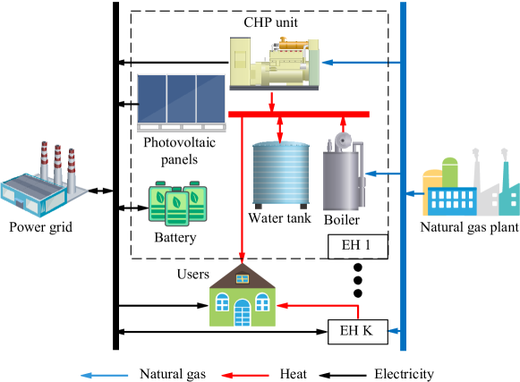
Figure 1: Energy flows of the industrial park

2.1 Energy Hub

In this subsection, the model of EH $k$, which consists of battery $k$, water tank $k$, CHP $k$ and boiler $k$, is given, where one time slot denotes one hour.

2.1.1 Battery and Water Tank

The battery $k$ and water tank $k$ are modeled as

$$B_{k}(t+1)=B_{k}(t)+\eta_{cke}C_{ke}(t)-\frac{1}{\eta_{dke}}D_{ke}(t)$$ (1)

$$W_{k}(t+1)=W_{k}(t)+\eta_{ckh}C_{kh}(t)-\frac{1}{\eta_{dkh}}D_{kh}(t)$$ (2)

$$B_{k,min}\leq B_{k}(t)\leq B_{k,max},W_{k,min}\leq W_{k}(t)\leq W_{k,max}$$ (3)

$$0\leq C_{ke}(t)\leq C_{ke,max},0\leq D_{ke}(t)\leq D_{ke,max}$$ (4)

$$0\leq C_{kh}(t)\leq C_{kh,max},0\leq D_{kh}(t)\leq D_{kh,max}$$ (5)

The battery power $B_{k}(t+1)$ at time slot $t+1$ is equal to the battery power $B_{k}(t)$ at time slot $t$ plus the charge amount $\eta_{cke}C_{ke}(t)$ minus the discharge amount $\frac{1}{\eta_{dke}}D_{ke}(t)$. The thermal energy of water tank $W_{k}(t+1)$ at time slot $t+1$ is equal to the thermal energy of water tank $W_{k}(t)$ at time slot $t$ plus the charge amount $\eta_{ckh}C_{kh}(t)$ minus the discharge amount $\frac{1}{\eta_{dkh}}D_{kh}(t)$.

2.1.2 CHP and Boiler

The models of CHP unit $k$ and boiler $k$ are expressed by

$$E_{kCHP}(t)=\eta_{kpg}G_{kCHP}(t),H_{kCHP}(t)=\eta_{khg}G_{kCHP}(t)$$ (6)

$$0\leq E_{kCHP}(t)\leq E_{kCHP,max},0\leq H_{kCHP}(t)\leq H_{kCHP,max}$$ (7)

$$H_{kb}(t)=\eta_{kbg}G_{kb}(t)$$ (8)

$$0\leq H_{kb}(t)\leq H_{kb,max}$$ (9)

CHP $k$ generates electricity $E_{kCHP}(t)$ and thermal energy $H_{kCHP}(t)$ by utilizing gas $G_{kCHP}(t)$. Boiler $k$ generates thermal energy $H_{kb}(t)$ by utilizing gas $G_{kb}(t)$. The corresponding conversion efficiencies are $\eta_{kpg}$, $\eta_{khg}$ and $\eta_{kbg}$.

2.2 Energy Trading with the Electricity and Gas Companies

The park purchases electricity $E(t)$ and gas $G(t)$ from utility companies to supply demand, respectively. When there is extra renewable energy, the excess electricity $E_{o}(t)$ can be sold to the company.

$$0\leq E(t)\leq E_{max},0\leq G(t)\leq G_{max},0\leq E_{o}(t)\leq E_{o,max}$$ (10)

2.3 Energy Load

The total available electricity $E_{tot}(t)$, heat $H_{tot}(t)$ and gas $G_{tot}(t)$ for industrial users is denoted as

$$E_{tot}(t)=\sum_{k\in\boldsymbol{K}}E_{kCHP}(t)+D_{ke}(t)-C_{ke}(t)+R_{k}(t)+E(t)-E_{o}(t)$$ (11a)

$$G_{tot}(t)=G(t)-\sum_{k\in\boldsymbol{K}}[G_{kCHP}(t)+G_{kb}(t)]$$ (11b)

$$H_{tot}(t)=\sum_{k\in\boldsymbol{K}}H_{kCHP}(t)+H_{kb}(t)+D_{kh}(t)-C_{kh}(t)$$ (11c)

The total electrical load is supplied by CHP units, batteries, renewable energy $R_{k}(t)$ and the power company. The total gas load is supplied by gas company. The total heat load is supplied by CHP units, boilers and water tanks.

The electrical loads include IL and EL. The IL, such as industrial production demands, refrigerators and illuminations, will not change easily over time. The EL, such as air conditioners, electric vehicles and gas water heaters, can be flexibly arranged. The number of IL users is $\boldsymbol{I}=\{1,2,...,I\}$ and the number of EL types is $\boldsymbol{Q}=\{1,2,...,Q\}$. The available energy of EH $k$ is expressed by:

$$0\leq x_{k}(t)\leq x_{k,max}$$ (12)

$$x_{k}(t)=\sum_{i\in\boldsymbol{I}}x_{ki}(t)+\sum_{q\in\boldsymbol{Q}}x_{kq}(t)$$ (13)

where $x_{k}(t)$ denotes the energy generation of EH $k$ with energy $x\in\boldsymbol{X}$, and $\boldsymbol{X}=\{E,H\}$, i.e., a set of electricity and heat. $x_{ki}(t)$ denote the IL of user $i$ supplied by EH $k$. $x_{kq}(t)$ denote the EL $q$ of users supplied by EH $k$.

2.4 Incentive Mechanism

Some electrical IL, such as illuminations and inefficient tertiary industrial demands, can be partially shifted when necessary, the industrial park will offer incentive price $p(t^{\prime})$ to shift electrical IL of user $i$ by an amount ${X}_{ir}(t^{\prime}-t)=r_{i}(p(t^{\prime}),(t^{\prime}-t)){X}_{i}(t)$ from $t$ to $t^{\prime}$ without compromising basic demand, where $r_{i}\leq\eta$ denotes the shifting probability of original electrical IL ${X}_{i}(t)$ of user $i$. The electrical IL of user $i$ shifted from $t$ is ${X}_{ir}(t)=\sum_{t^{\prime}\neq t}X_{ir}(t^{\prime}-t)=\sum_{t^{\prime}\neq t}r_{i}(p(t^{\prime}),(t^{\prime}-t)){X}_{i}(t)$.

Thus, the cost of offering incentive for the shifted electrical IL of user $i$ from $t$ is denoted as

$$\sum_{t^{\prime}\neq t}p(t^{\prime}){X}_{ir}(t^{\prime}-t)$$ (14)

To estimate the shifting functions, a form of given function with adjustable parameters is introduced [22]. The shifting function $r$ is regarded to exponentially decrease in time and increase in incentive amount:

$$r_{\alpha_{i}}(p,t)=C_{\alpha_{i}}\frac{p}{(t+1)^{\alpha_{i}}}$$ (15)

where $C_{\alpha_{i}}$ is a constant which depends on $\alpha_{i}$. The parameter $\alpha_{i}$ denotes the willingness of user $i$ to shift IL. The higher $\alpha_{i}$, the shorter the time user $i$ is willing to shift its demand. The shifting function can be an approximation of the nonlinear mode of user behavior.

To estimate $\alpha_{i}$ for each user, all $\alpha_{i}$ at a time slot are integrated in one integral shifting function, which sums the shifting functions of all users at that time slot, weighted based on the percentage of electricity consumed by each user. The integral shifting function at time slot $t$ is denoted as:

$$R(p,t)=\sum_{i\in\boldsymbol{I}}\beta_{i}r_{i}(p,t)$$ (16)

where $\beta_{i}$ is the percentage of electricity consumed by user $i$. The amount of electricity demand shifted from $t$ to $t^{\prime}$ is:

$$A_{t,t^{\prime}}=X_{IL}(t)R(p(t^{\prime}),(t^{\prime}-t))$$ (17)

where ${X}_{IL}(t)$ is the original electrical IL of all users at time slot $t$.

The difference $J_{t}$ between the original demand and the demand after offering incentive at time slot $t$, which can be obtained directly from historical data in large quantities, is denoted as:

$$J_{t}=\sum_{t^{\prime}\neq t}A_{t^{\prime},t}-A_{t,t^{\prime}}$$ (18)

Since $t=0,1,...,T-1$, each $J_{t}$ is denoted as a linear function of multiple $A_{t^{\prime},t}$. Based on the values from $J_{0}$ to $J_{T-1}$, these linear expressions can be solved for $A_{t,t^{\prime}}$.

According to $A_{t,t^{\prime}}=X_{IL}(t)\sum_{i\in\boldsymbol{I}}\beta_{i}C_{\alpha_{i}}\frac{p(t^{\prime})}{(t^{\prime}+1)^{\alpha_{i}}}$, we assume that $Y(t)=\sum_{i\in\boldsymbol{I}}\beta_{i}C_{\alpha_{i}}\frac{p(t)}{(t+1)^{\alpha_{i}}}$. The error sum of squares is denoted as

$$E_{Y}=\sum_{t^{\prime}\neq t}(Y(t^{\prime})-\sum_{i\in\boldsymbol{I}}\beta_{i}C_{\alpha_{i}}\frac{p(t^{\prime})}{(t^{\prime}+1)^{\alpha_{i}}})^{2}$$

Letting $y_{i}(t)=\frac{\beta_{i}C_{\alpha_{i}}}{(t^{\prime}+1)^{\alpha_{i}}}$, we have $\ln y_{i}(t)=\ln C_{\alpha_{i}}+\ln\beta_{i}-{\alpha_{i}}\ln(t+1)$. In real situation, when $p(t^{\prime})$ is set, $J_{t}$ and $X_{IL}(t)$ can be obtained from electric meter. Taking the derivative of $E_{Y}$ with respect to $y_{i}(t^{\prime})$,

$$\frac{\partial E_{Y}}{\partial y_{i}(t^{\prime})}=\sum_{t^{\prime}\neq t}2(Y(t^{\prime})-\sum_{i\in\boldsymbol{I}}y_{i}(t^{\prime})p(t^{\prime}))Ip(t^{\prime})$$ (19)

${y_{i}(t^{\prime})}$ can be obtained by setting the derivative (19) equal to zero. Then taking the derivative of $E_{y}=\sum_{i\in\boldsymbol{I}}(\ln y_{i}(t)-\ln C_{\alpha_{i}}-\ln\beta_{i}+{\alpha_{i}}\ln(t+1))^{2}$ with respect to $\alpha_{i}$ and $\ln\beta_{i}$, respectively

$$\frac{\partial E_{y}}{\partial\alpha_{i}}=\sum_{i\in\boldsymbol{I}}2(\ln y_{i}(t)-\ln C_{\alpha_{i}}-\ln\beta_{i}+{\alpha_{i}}\ln(t+1))\ln(t+1)$$ (20)

$$\frac{\partial E_{y}}{\partial\ln\beta_{i}}=\sum_{i\in\boldsymbol{I}}-2(\ln y_{i}(t)-\ln C_{\alpha_{i}}-\ln\beta_{i}+{\alpha_{i}}\ln(t+1))$$

By setting the derivative (20) equal to zero, we can obtain $\alpha_{i}$ and $\beta_{i}$ which give the shifting functions offline.

3 Solution Method

In this paper, a stochastic gradient-based scheduling method is adopted to minimize the time average cost. All random variables are integrated into $\boldsymbol{r}(t)=\{R(t),X(t)\}$, and all optimization variables are integrated into $\boldsymbol{M}(t)$={$x_{ki}(t)$, $x_{kq}(t)$, $x_{k}(t)$, $D_{ke}(t)$, $C_{ke}(t)$, $D_{kh}(t)$, $C_{kh}(t)$, $E_{o}(t)$, $E(t)$, $G(t)$, $p(t)$}. The total cost of the park at time slot $t$ is expressed as

$$\phi(t) =E(t)p_{e}(t)+G(t)p_{g}(t)-E_{o}(t)p_{o}(t)$$ (21)

$$+\sum_{i\in\boldsymbol{I}}(\sum_{t^{\prime}\neq t}p(t^{\prime}){X}_{ir}(t^{\prime}-t)-U_{i}(t))-\sum_{k\in\boldsymbol{K}}\sum_{q\in\boldsymbol{Q}}U_{kq}(t)$$

where $U_{i}(t)=a_{ii}(X_{i}(t)-{X}_{ir}(t))^{2}+b_{ii}(X_{i}(t)-{X}_{ir}(t))$ and $U_{kq}(t)=a_{kq}x_{kq}^{2}(t)+b_{kq}x_{kq}(t)$. $a_{ii}$, $b_{ii}$, $a_{kq}$ and $b_{kq}$ are the corresponding utility coefficients. $p_{e}(t)$ and $p_{g}(t)$ denote the electricity price and gas price of the companies, respectively. $p_{o}(t)$ denotes the electricity price sold to the power company. $U_{i}(t)$ and $U_{kq}(t)$ denote the satisfaction income of IL of user $i$ and EL $q$ provided by EH $k$.

The energy management problem of the park is to find a method to minimize the time average energy cost:

$$\min_{\boldsymbol{M}(t)}\lim_{T\rightarrow\infty}\frac{1}{T}\sum_{t=0}^{T-1}\mathbb{E}\{\phi(t)\}$$ (22)

$$\text{s.t. }(\ref{A1})-(\ref{eqdt})$$

where the expectation is taken for all uncertain variables.

Some methods in the following subsections are adopted to make the optimization problem easier to solve. Fig. 2 shows the problem-solving process.

Figure 2: Problem-solving process

3.1 Constraints Replacement

The optimization variables are coupled in the battery dynamics (1) and water tank dynamics (2), and cannot be obtained directly. Moreover, considering that it is causal for the knowledge of the random variable $\boldsymbol{r}(t)$, the optimization problem of cross-time coupling is usually difficult to tackle. To handle this issue, we replace the temporally-coupled constraints (1) and (2) with the time-average constraints.

According to (1)-(3), the average energy charge and discharge can be denoted by

$$\lim_{T\rightarrow\infty}\frac{1}{T}\sum_{t=0}^{T-1}\mathbb{E}\{C_{ke}(t)\}=\lim_{T\rightarrow\infty}\frac{1}{T}\sum_{t=0}^{T-1}\mathbb{E}\{D_{ke}(t)\}$$ (23a)

$$\lim_{T\rightarrow\infty}\frac{1}{T}\sum_{t=0}^{T-1}\mathbb{E}\{C_{kh}(t)\}=\lim_{T\rightarrow\infty}\frac{1}{T}\sum_{t=0}^{T-1}\mathbb{E}\{D_{kh}(t)\}$$ (23b)

where (23b) can guarantee that the charged energy is equal to the discharged energy for a long period. Based on (23b), the optimization problem (22) can be relaxed as

$$\min_{\boldsymbol{M}(t)}\lim_{T\rightarrow\infty}\frac{1}{T}\sum_{t=0}^{T-1}\mathbb{E}\{\phi(t)\}$$ (24)

$$\text{s.t. }(\ref{Cem})-(\ref{eqdt}),(\ref{sto1})$$

Compared with (22) , time-coupling constraints (1) and (2) are superseded by (23b). If the stochastic process $\boldsymbol{r}(t)$ is stationary, the time-invariant control strategy $\boldsymbol{M}:\boldsymbol{r}(t)\rightarrow\boldsymbol{M}(t)$ induces the solution $\boldsymbol{M}(t)=\boldsymbol{M}(\boldsymbol{r}(t))$, which can satisfy the constraint condition (4) - (13) and (23b), and achieve the optimal performance [23]. This means that all expectations of the limiting time-averaged in (24) produce the same result. Thus, the time-averaged can be removed. To deal with the coupling introduced by the expectation in (23b), the constraints (23b) are dualized and the dual decomposition method is used. After the dualization, the solution can be computed separately across time, which will be illustrated in the following section.

3.2 Stochastic Energy Optimization

First, Lagrangian multiplier method is used to deal with the coupling constraint (23b). The Lagrangian function about (24) is denote as

$$L(\boldsymbol{M}(t),\boldsymbol{\lambda}) =\mathbb{E}\{\phi(t)\}+\sum_{k\in\boldsymbol{K}}\mathbb{E}[\lambda_{ke}(C_{ke}(t)-D_{ke}(t))]$$ (25)

$$+\sum_{k\in\boldsymbol{K}}\mathbb{E}[\lambda_{kh}(C_{kh}(t)-D_{kh}(t))]$$

where $\lambda_{ke}$ and $\lambda_{kh}$ are the corresponding Lagrangian multipliers.

The corresponding Lagrangian dual function is denoted as

$$\Gamma(\boldsymbol{\lambda}) =\min_{\boldsymbol{M}(t)\in\widetilde{\boldsymbol{M}}(t)}L(\boldsymbol{M}(t),\boldsymbol{\lambda})$$ (26)

where $\widetilde{\boldsymbol{M}}(t)$ denotes the solution under constraints (4) - (13). The corresponding dual problem is expressed by

$$\max_{\boldsymbol{\lambda}}\Gamma(\boldsymbol{\lambda})$$ (27)

A gradient algorithm is introduced to obtain the optimal solution $\boldsymbol{\lambda}^{*}$ of problem (27). The Lagrangian multipliers $\boldsymbol{\lambda}(t+1)$ at time slot $t+1$ are expressed by

$$\lambda_{ke}(t+1)=\lambda_{ke}(t)+\rho(C_{ke}(t)-D_{ke}(t))$$ (28a)

$$\lambda_{kh}(t+1)=\lambda_{kh}(t)+\rho(C_{kh}(t)-D_{kh}(t))$$ (28b)

where $C_{ke}(t)$, $D_{ke}(t)$, $C_{kh}(t)$ and $D_{kh}(t)$ can be acquired by solving

$$\Phi^{*} =\min_{M(t)}\Phi(t)=\min_{M(t)}\phi(t)+\sum_{k\in\boldsymbol{K}}[\lambda_{ke}(t)(C_{ke}(t)$$ (29)

$$-D_{ke}(t))+\lambda_{kh}(t)(C_{kh}(t)-D_{kh}(t))]$$

$$\text{s.t. }(\ref{Cem})-(\ref{eqdt})$$

The stochastic iteration in (28b) and (29) has two advantages. First, the solution obtained by (29) approaches the solution to (24). Second, when initialized correctly, the solution of (29) can be feasible for original problem (22). These advantages will be elaborated in Section 4.

3.3 Fast Distributed Implementation

Although the original problem (22) is separated across time, it still requires a centralized method to solve the convex problem (29), which is challenging in the presence of a large number of variables. Therefore, it is necessary to obtain the optimal solution in a distributed algorithm [24], which aims to improve robustness and reduce computational complexity.

In this way, the dual decomposition method is introduced again to deal with the coupling between EL and IL for constraint (13) in (29). The IL should be satisfied immediately and the decision is real-time [25], so the fast distributed algorithm needs to run some iterations on mini-slots at each time slot. That is, the proposed algorithm runs on two timescales. The corresponding Lagrangian function on a fast timescale is expressed by

$$\overline{L}(\boldsymbol{M},\boldsymbol{\tau}):=\Phi(t)+\sum_{k\in\boldsymbol{K}}\tau_{k}(\sum_{i\in\boldsymbol{I}}x_{ki}+\sum_{q\in\boldsymbol{Q}}x_{kq}-x_{k})$$ (30)

where $\boldsymbol{\tau}=\{\tau_{1},...,\tau_{K}\}$ denotes the set of the corresponding Lagrangian multipliers, and the dual variable $\boldsymbol{\lambda}(t)$ in $\Phi(t)$ is updated on a slow timescale, i.e., $\boldsymbol{\lambda}(t)$ can be seen as constants to solve optimization problem (29). The corresponding dual function is expressed as

$$\overline{\Gamma}(\boldsymbol{\tau}):=\min_{\boldsymbol{M}\in\overline{\boldsymbol{M}}}\overline{L}(\boldsymbol{M},\boldsymbol{\tau})$$ (31)

where $\overline{\boldsymbol{M}}$ denotes the feasible solution under constraints (4) - (13). The corresponding dual problem is expressed by

$$\max_{\boldsymbol{\tau}}\overline{\Gamma}(\boldsymbol{\tau})$$ (32)

Unlike the dual problem (27), which implements stochastic estimation, (32) aims to schedule energy in a distributed manner for each EH and user. Next, two gradient-based methods will be used to solve the issue (32).

We first introduce the conventional gradient algorithm to find Lagrangian multipliers $\boldsymbol{\tau}$, and the iteration for $\boldsymbol{\tau}$ is expressed by

$$\boldsymbol{\tau}(n+1)=\boldsymbol{\tau}(n)+\sigma\nabla\overline{\Gamma}(\boldsymbol{\tau}(n))$$ (33)

where $n$ denotes the index of the mini-slot, and $\sigma$ denotes the stepsize. The gradient of ${\tau}_{k}(n)$ can be expressed as

$$\nabla\overline{\Gamma}(\tau_{k}(n))=\sum_{i\in\boldsymbol{I}}x_{ki}(n)+\sum_{q\in\boldsymbol{Q}}x_{kq}(n)-x_{k}(n)$$ (34)

Although conventional gradient algorithm has been universally used, it does not take advantage of the properties of the problem, i.e., the differentiability of the function and the Lipschitz continuity of the gradient, and its convergence rate is slow. To solve the problem online, a scheme is proposed to realize faster convergence than the conventional gradient algorithm based on a fast iterative algorithm [26].

Unlike the conventional gradient algorithm of (33), which only depends on the current iteration, the proposed fast method uses the memory of the previous iteration and constructs $\overline{\boldsymbol{\tau}}(n)$ by utilizing $\boldsymbol{\tau}(n)$ and $\boldsymbol{\tau}(n-1)$, which can be expressed as

$$\overline{\boldsymbol{\tau}}(n)=(1-\epsilon)\boldsymbol{\tau}(n)+\epsilon\boldsymbol{\tau}(n-1)$$ (35)

where $\epsilon=(1-\theta_{\tau}(n-1))/\theta_{\tau}(n)$, and $\theta_{\tau}(n)$ is updated as

$$\theta_{\tau}(n)=(1+\sqrt{1+4\theta^{2}_{\tau}(n-1)})/2$$ (36)

$\boldsymbol{\tau}(n)$ can be denoted using a gradient iteration about $\overline{\boldsymbol{\tau}}(n)$

$$\tau_{k}(n+1)=\overline{\tau}_{k}(n)+\sigma(\sum_{i\in\boldsymbol{I}}x_{ki}(n)+\sum_{q\in\boldsymbol{Q}}x_{kq}(n)-x_{k}(n))$$ (37)

According to (31), the optimal energy scheduling solution $\boldsymbol{M}(n)$ is obtained by solving

$$\min_{\boldsymbol{M}(n)} \,E(n)p_{e}(n)+G(n)p_{g}(n)-E_{o}(n)p_{o}(n)+\lambda_{ke}(n)(C_{ke}(n)-D_{ke}(n))$$ (38)

$$+\lambda_{kh}(n)(C_{kh}(n)-D_{kh}(n))-\tau_{k}(n)x_{k}(n)+\sum_{k\in\boldsymbol{K}_{i}}\tau_{k}(n)x_{ki}(n)$$

$$+\sum_{i\in\boldsymbol{I}}[\sum_{n^{\prime}\neq n}p(n^{\prime}){X}_{ir}(n^{\prime}-n)-U_{i}(n)]+\tau_{k}(n)x_{kq}(n)-U_{kq}(n)$$

$$\text{s.t. }(\ref{Cem})-(\ref{eqdt1})$$

According to the expression of $U_{i}(n)$,

$$\sum_{i\in\boldsymbol{I}}[\sum_{n^{\prime}\neq n}p(n^{\prime}){X}_{ir}(n^{\prime}-n)-U_{i}(n)]=\sum_{i\in\boldsymbol{I}}[\sum_{n^{\prime}\neq n}p(n^{\prime})X_{i}(n)r_{i}(p(n^{\prime}),(n^{\prime}-n))$$ (39)

$$-a_{ii}X^{2}_{i}(n)(1-\sum_{n^{\prime}\neq n}r_{i}(p(n^{\prime}),(n^{\prime}-n)))^{2}+b_{ii}X_{i}(n)(1-\sum_{n^{\prime}\neq n}r_{i}(p(n^{\prime}),(n^{\prime}-n)))]$$

For simplicity, $r_{i}(p(n^{\prime}),(n^{\prime}-n))$ is written as $r_{i}$. According to (15), $r_{i}$ and $p(n^{\prime})$ are linearly related, and $r_{i}=p(n^{\prime})\frac{\partial r_{i}}{\partial p(n^{\prime})}$. Taking the derivative of (38) with respect to $p(n^{\prime})$ yields

$$\sum_{i\in\boldsymbol{I}}[2p(n^{\prime})\frac{\partial r_{i}}{\partial p(n^{\prime})}X_{i}(n)+2a_{ii}X^{2}_{i}(n)(1-p(n^{\prime})\frac{\partial r_{i}}{\partial p(n^{\prime})})\frac{\partial r_{i}}{\partial p(n^{\prime})}$$ (40)

$$-b_{ii}X_{i}(n)\frac{\partial r_{i}}{\partial p(n^{\prime})}]=0$$

$p(n^{\prime})$ can be denoted by

$$p(n^{\prime})=\frac{\sum_{i\in\boldsymbol{I}}(X_{i}(n)\frac{\partial r_{i}}{\partial p(n^{\prime})})(2a_{ii}X_{i}(n)-b_{ii})}{\sum_{i\in\boldsymbol{I}}(X_{i}(n)\frac{\partial r_{i}}{\partial p(n^{\prime})})(2a_{ii}X_{i}(n)\frac{\partial r_{i}}{\partial p(n^{\prime})}-2)}$$

Considering that (29) satisfies the Slater condition and is convex, the solution obtained by (32) is feasible for the original problem (29). When $\rho$ is properly chosen, the iterations (33) and (37) will converge to the vicinity of $\boldsymbol{\tau}^{*}$, and the obtained solution can be made arbitrarily close to the optimal value [27].

The proposed fast method is shown in Algorithm 1, which incurs low complexity. Updating (28b) only requires complexity $\mathcal{O}(K)$, and the complexity of worst-case for solving (38) is $\mathcal{O}(I(I^{2}+K^{3}))$. By combining the two consecutive iterations, the constructed iteration $\overline{\tau}(n)$ achieves faster convergence by reducing the undesired fluctuation of the gradient ascent method without compromising accuracy. The convergence of Algorithm 1 needs to meet two conditions: 1) the dual function $\overline{\Gamma}(\boldsymbol{\tau})$ is differentiable; 2) the gradient $\nabla\overline{\Gamma}$ is Lipschitz continuous. In practice, marginal costs are usually monotonic, which guarantee that the cost function $\phi(t)$ is strongly convex about $\boldsymbol{M}(t)$. For a given $\boldsymbol{\tau}$, the Lagrangian function (30) has a unique minimizer. Therefore, the dual function $\overline{\Gamma}(\boldsymbol{\tau})$ is differentiable and the gradient $\nabla\overline{\Gamma}$ is Lipschitz continuous.

The detailed proof of condition 1) can be found in [28], and the detailed proof of condition 2) can be found in [29].

Algorithm 1 Fast Method

1:Initialize: $\boldsymbol{\tau}(0)$, $\boldsymbol{\tau}(1)$, $\theta_{\tau}(0)$ and $\sigma$.

2:for each mini-slot $n$ do

3:    Calculate $\theta_{\tau}(n)$ based on (36).

4:    Calculate $\overline{\boldsymbol{\tau}}(n)$ according to (35).

5:    EHs send $\overline{\boldsymbol{\tau}}(n)$ to users.

6:    Each user and EH obtain the solution $\boldsymbol{M}(n)$ using $\boldsymbol{\tau}=\overline{\boldsymbol{\tau}}$ according to (38).

7:    Update $\boldsymbol{\tau}(n+1)$ based on (37).

The proposed fast distributed algorithm, which combines the dual decomposition and the fast method, is shown in Fig. 3.

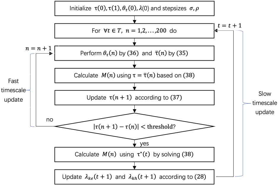
Figure 3: Flow chart of the proposed algorithm

4 Performance Analysis

To enable the proposed algorithm to generate feasible strategy for (22), the following properties are given:

Lemma 1. The charge and discharge of the battery satisfy: 1) When $\lambda_{ke}(t)>-{p}_{o}(t)$, $D_{ke}(t)={D}_{ke,max}$ ; 2) When $\lambda_{ke}(t)<-{p}_{e}(t)$, $C_{ke}(t)={C}_{ke,max}$. The equivalent thermal energy of charge and discharge of the water tank satisfy: 1) When $\lambda_{kh}(t)>0$, $D_{kh}(t)={D}_{kh,max}$; 2) When $\lambda_{kh}(t)<0$, $C_{kh}(t)={C}_{kh,max}$.

For brevity, the proof is omitted. Please refer to Ref. [30].

Lemma 1 states that the Lagrangian multiplier $\lambda_{ke}(t)$ can be regarded as a charge price. When $\lambda_{ke}(t)$ is low enough, the battery will charge as it can. When $\lambda_{ke}(t)$ is high enough, the battery will discharge as it can. According to Lemma 1, the result can be determined as follows:

Lemma 2. If $\rho\geq{\rho_{min}}$, where ${\rho}_{min}=\max_{k}\frac{{p}_{e,max}-{p}_{o,min}}{{B}_{k,max}-{B}_{k,min}-{D}_{ke,max}-{C}_{ke,max}}$, Lagrangian multipliers $\lambda_{ke}(t)$ and $\lambda_{kh}(t)$ satisfy $-{p}_{e,max}-\rho{D}_{ke,max}\leq\lambda_{ke}(t)\leq\rho{B}_{k,max}-\rho{B}_{k,min}-{p}_{e,max}-\rho{D}_{ke,max}$ and $-\rho{D}_{kh,max}\leq\lambda_{kh}(t)\leq\rho{W}_{k,max}-\rho{W}_{k,min}-\rho{D}_{kh,max}$.

The proof of this step is shown in Appendix A.

According to Lemma 2, when $B_{k}(t)=(\lambda_{ke}(t)+{p}_{e,max})/\rho+{B}_{k,min}+D_{ke,max}$ and $W_{k}(t)=\lambda_{kh}(t)/\rho+{W}_{k,min}+D_{kh,max}$, ${B}_{k,min}\leq{B}_{k}\leq{B}_{k,max}$ and ${W}_{k,min}\leq{W}_{k}\leq{W}_{k,max}$, i.e., the capacity constraints of the battery and water tank are always satisfied.

Based on Lemma 2, the performance of the fast distributed algorithm can be obtained.

Theorem 1. When the random state $\boldsymbol{r}(t)$ is i.i.d, $\lambda_{ke}(0)=\rho{B}_{k}(0)-\rho{B}_{k,min}-{p}_{e}(0)-\rho{D}_{ke,max}$, and $\rho\geq{\rho_{min}}$, the expected time-averaged cost under the fast distributed algorithm satisfies

$$\lim_{T\rightarrow\infty}\frac{1}{T}\sum_{t=0}^{T-1}\mathbb{E}\{\phi(t)\}\leq\phi^{*}+\rho F$$ (41)

where $\phi^{*}$ is the optimal cost of (22), and $F$ is defined by

$$F=\frac{1}{2}(\max({C}_{ke,max},{D}_{ke,max}))^{2}+\frac{1}{2}(\max(C_{kh,max},D_{kh,max}))^{2}$$ (42)

Proof: For brevity, the proof is omitted here. Please refer to Ref. [30].

Theorem 1 shows the gap between the performance of the fast distributed algorithm and the optimal performance. The gap increases with $\rho$. According to Lemma 2, it can be concluded that the smaller ${p}_{e,max}-{p}_{o,min}$, the smaller $\rho$. Similarly, the larger $B_{k,max}$ in Lemma 2, the smaller $\rho$. Therefore, when ${p}_{e,max}-{p}_{o,min}$ is made close to zero or $B_{k,max}$ is large, the stepsize $\rho$ will be small enough and the gap will be close to zero.

5 Case Studies

We give numerical results based on actual data to evaluate the performance of proposed algorithm .

5.1 Simulation Setup

Three factories and two EHs are considered in the industrial park. Each EH has a battery, a hot water tank, a CHP unit and a boiler. Each factory has one kind of electrical EL and IL, gas and heat loads, respectively. For simplicity, the three kinds of electrical EL in the three factories are calculated together and shown as a whole in the simulation figure. The coefficients of the same type of equipment and load are set to be the same. For example, energy conversion coefficients of two boilers are both $\eta_{kbg}=85\%$. The same assumption is available for batteries, water tanks, CHP units, ILs and ELs. The ratio of maximum electrical IL shifting is $\eta=0.15$, and the gas price is $p_{g}(t)=0.4$ ¥/kWh. Other relevant parameters are shown in Table 1, and the parameter settings are similar to Ref. [31]. The adjustment of the parameters will not affect the simulation results.

Table 1: Relevant Parameters

Parameter	Value	Parameter	Value
$B_{k,max}$,$W_{k,max}$	4MWh	$a_{ii}$,$a_{kq}$	-1
$C_{kh,max}$,$D_{kh,max}$	1MWh	$b_{ii}$	1
$C_{ke,max}$,$D_{ke,max}$	1MWh	$b_{kq}$	7
$\eta_{kpg}$	35%	$\eta_{khg}$	45%
$\eta_{cke}$,$\eta_{dke}$	98%	$\eta_{ckh}$,$\eta_{dkh}$	98%

Three different cases are used for comparison to evaluate the proposed algorithm: Case 1 is a stochastic optimization algorithm with two-timescale (denoted as TA), which is similar to the algorithm of [32], where there is no energy storage. Case 2 is an algorithm based on stochastic gradient without renewable energy resource (denoted as OA), which is similar to the algorithm of [33]. To verify the effectiveness of the incentive mechanism, Case 3, a censored version of the proposed algorithm (denoted as CA) without incentive mechanism, is utilized for comparison. Fig. 4 (a) shows the electricity price of JiangSu Electric Power Company [34]. Fig. 4 (b) shows the hourly load of factories from PJM [35].

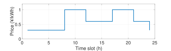
(a) Electricity price of the power company

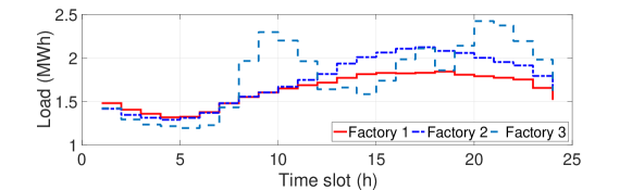
(b) Electrical load of factories

Figure 4: Data from website.

5.2 Performance Verification

In order to confirm the performance analyzed in Section 4, the following two situations need to be considered. Situation 1: When renewable energy is sufficient (assumed to be six times the original renewable energy), the industrial park will have excess energy to sell. In this situation, the adjusted sales price ${p_{o}(t)}$ is proportional to the purchase price ${p_{e}(t)}$. Table 2 shows that the smaller the $\frac{p_{e}(t)}{p_{o}(t)}$, the smaller the total cost. Situation 2: In current industrial production, there is no surplus energy in the industrial park to sell to the public utility company, and renewable energy cannot meet the total demand of factories at all time. In this situation, the purchase price ${p_{e}(t)}$ is adjusted. Table 2 shows that the smaller $p_{e,max}-p_{o,min}$, the smaller the total cost. These two situations are consistent with Lemma 2 and Theorem 1, where the cost gap increases with $\rho$.

Table 2: The impact of the price variance on the total cost (¥)

$\frac{p_{e}(t)}{p_{o}(t)}$	2	1.9	1.8	1.7	1.6	1.5	1.4	1.3	1.2	1.1	1
Cost ($*10^{3}$)	94.1	93.4	92.7	92.0	91.2	89.6	88.2	86.7	84.7	81.9	78.4

$p_{e,max}-p_{o,min}$	0.9	0.8	0.7	0.6	0.5	0.4	0.3	0.2	0.1
Cost ($*10^{3}$)	141.5	135.9	130.0	123.5	116.4	107.3	97.5	86.7	75.2

The following simulation settings follow the previous subsection. The convergence of the solution to problem (29) is shown in Table 3 and Fig. 5. Table 3 shows the number of iterations for different methods during 12 hours. The comparison of the cumulative distribution function (CDF) about the number of iterations for different methods at $t=1$ is shown in Fig. 5 (a). Then, the comparison time is increased to $T=360$ slots to further illustrate the results, and each time slot can only consider up to 200 mini-slots. The iteration will not be stopped until the difference between two iterations is less than 0.01 or the number of iteration for (29) is greater than 200. Both the fast method (37) and the conventional gradient algorithm (33) have an iterative stepsize of $\sigma=0.2$. According to Fig. 5 (b), the iteration number of the fast method is about 20, while the conventional gradient algorithm requires more than 40 iterations to converge in most cases. Therefore, by combining two previous iterations, the fast method reduces the undesired fluctuations of the gradient iteration to realize rapid convergence.

Table 3: The number of iterations for different methods during 12 hours

$t(h)$	1	2	3	4	5	6	7	8	9	10	11	12
Fast Method	15	20	24	18	24	17	21	23	22	22	22	15
Gradient	42	40	49	37	50	33	41	73	70	70	70	29

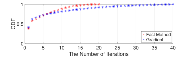
(a) The comparison of CDF about the number of iterations.

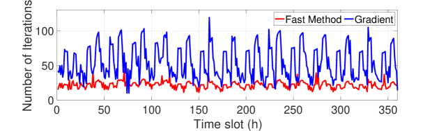
(b) The number of iterations for different methods across 360 time slots.

Figure 5: Comparison for different methods.

Table 4 shows the comparison of the total costs for different methods. Fig. 6 shows the comparison of the costs across 24 time slots for different methods. The cost of the proposed algorithm is lower than that of TA, OA and CA. Due to the lack of energy storage, TA needs to purchase more electricity instead of discharging during peak periods and is sensitive to the high electricity price and renewable energy consumption. Due to the lack of incentive mechanism and EL, CA is sensitive to changes in prices, renewable energy and loads. Therefore, the park needs to pay higher costs under TA/CA. The effect of OA approaches the proposed algorithm during 0:00-6:00 and 20:00-24:00, but it needs to buy more energy in daytime due to the lack of renewable energy in OA. Since TA, OA and CA need to purchase more high-priced electricity from the grid during peak demand, their costs are higher. The comparison of total costs between the proposed algorithm and TA shows that the cost is improved 6.17% by the energy storage, and the comparison of total costs between the proposed algorithm and OA shows that the cost is improved 7.23% through introducing renewable energy resource, and the comparison of total costs between the proposed algorithm and CA shows that the cost is improved 8.16% by incentive mechanism. Therefore, the proposed fast distributed algorithm takes full advantage of incentive mechanism and the characteristic of loads to coordinate multi-energy, and utilizes batteries, water tanks and distributed energy generation to minimize the total cost of the industrial park online.

Table 4: Comparison of total costs for different methods (¥)

Methods	Proposed algorithm	TA	OA	CA
Cost ($*10^{3}$)	138.5	147.6	149.3	150.8

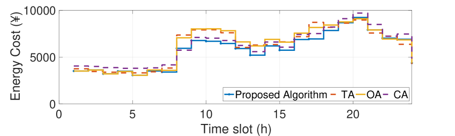
Figure 6: Comparison of costs across 24 time slots for different methods.

Figs.  7-9 show the energy generation/discharging and consumption/charging of the park, where the data of photovoltaic systems is provided by Renewables.ninja [36]. As the price of electricity sold by the power company changes over time, the CHP units are introduced to output electricity rather than buying the high-priced electricity, and supplying heat to the industrial park at the same time, as shown in Figs.  7-9. Fig. 7 shows that the batteries are discharged when the electricity price is high, such as 8:00, 9:00 and 17:00, and charged when the electricity price is low, such as 12:00, 14:00 and 21:00. In addition, according to Fig. 7, users have less EL under high electricity price. When the heat generated by CHP units cannot meet the demand, the boilers meet the unmet demand, as shown in Figs. 8 and 9. Figs. 7-9 show that the proposed fast distributed algorithm achieves energy transactions with power and gas companies, multi-energy demand shift, and flexible supply of energy through energy storage. Therefore, the proposed algorithm can realize the time-average cost that is close to the optimal cost and ensure real-time coordination and fast convergence.

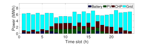
(a) Power generation/discharging

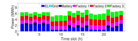
(b) Power consumption/charging

Figure 7: Power distribution profiles of the park.

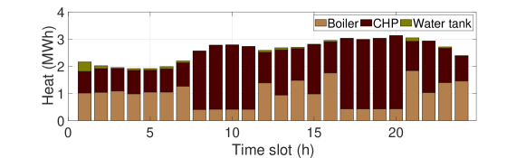
(a) Heat generation/discharging

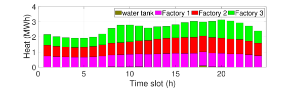
(b) Heat consumption/charging

Figure 8: Heat distribution profiles of the park.

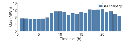
(a) Gas purchase

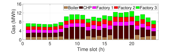
(b) Gas consumption

Figure 9: Gas distribution profiles of the park.

6 Conclusion

In this paper, the energy management problem of a multi-energy industrial park is investigated, which is an imperative issue of today’s industrial production. A systematic online energy cost minimization framework composed of energy hubs and users is presented, which makes full use of the adjustment mechanism of elastic load, the compensation mechanism of inelastic load and the coordination mechanism of multi source-load-storage. An incentive mechanism is implemented by estimating users’ willingness to shift peak loads without knowing information of each individual user. The energy scheduling issue is constructed as a two-timescale optimization problem, which can further consider the temporal and spatial changes of renewable energy, load and electricity prices, to achieve energy storage balancing and real-time load balancing while respecting energy constraints. A fast distributed algorithm based on two-stage dual decomposition is proposed to deal with temporally-coupled constraints and ensure real-time coordination of instantaneous scheduling. Finally, the performance and feasibility of the proposed algorithm are verified by theoretical analysis and case studies.

In this paper, an industrial park consists of two energy hubs and three factories. According to actual industrial scenarios, a park can have many generation plants and factories. Therefore, the scale and characteristics of the park need to be further considered. Investigating some diversified multi-energy management frameworks, such as Ref. [37], to solve the practical problems of multi-energy market is an important line of inquiry. Another line is to design some management schemes, like Ref. [38], to further explore the deployment of battery and thermal energy storage to improve energy efficiency.

Appendix A Proof of Lemma 2

The induction is used to prove Lemma 2. First, the conditions hold at time 0 and still hold at time $t$. Then, the following three cases are considered.

1. Case 1: $\lambda_{ke}(t)\in[-p_{o,min},\rho B_{k,max}-\rho B_{k,min}-p_{e,max}-\rho D_{ke,max}]$, where $p_{o,min}=\min\{p_{o}(t),\forall t\}$, and $p_{e,max}=\max\{p_{e}(t),\forall t\}$. In this case, according to Lemma 2, $C_{ke}(t)=0$ and $D_{ke}(t)=D_{ke,max}$. Since $-p_{e,max}<-p_{o,min}$, $\lambda_{ke}(t+1)=\lambda_{ke}(t)+\rho(C_{ke}(t)-D_{ke}(t))\in[-p_{e,max}-\rho D_{ke,max},\\ \rho B_{k,max}-\rho B_{k,min}-p_{e,max}-\rho D_{ke,max}]$.

2. Case 2: $\lambda_{ke}(t)\in[-p_{e,max},-p_{o,min}]$. In this case, since $\rho\geq\rho_{min}$, $\lambda_{ke}(t+1)=\lambda_{ke}(t)+\rho(C_{ke}(t)-D_{ke}(t))\in[-p_{e,max}-\rho D_{ke,max},-p_{o,min}+\rho C_{ke,max}]\subseteq[-p_{e,max}-\rho D_{ke,max},\rho B_{k,max}-\rho B_{k,min}-p_{e,max}-\rho D_{ke,max}]$.

3. Case 3: $\lambda_{ke}(t)\in[-p_{e,max}-\rho D_{ke,max},-p_{e,max}]$. In this case, according to Lemma 2, $C_{ke}(t)=C_{ke,max}$ and $D_{ke}(t)=0$. Since $-p_{e,max}<-p_{o,min}$ and $C_{ke,max}>0$, $\lambda_{ke}(t+1)=\lambda_{ke}(t)+\rho(C_{ke}(t)-D_{ke}(t))\in[-p_{e,max}-\rho D_{ke,max}+\rho C_{ke,max},-p_{e,max}+\rho C_{ke,max}]\subseteq[-p_{e,max}-\rho D_{ke,max}+\rho C_{ke,max},\\ -p_{o,min}+\rho C_{ke,max}]\subseteq[-p_{e,max}-\rho D_{ke,max},\rho B_{k,max}-\rho B_{k,min}-p_{e,max}-\rho D_{ke,max}]$.

It is similar to analyze $\lambda_{kh}(t)$.

References

- [1] Y. Liu, B. Xu, A. Botterud, N. Zhang and C. Kang, ”Bounding Regression Errors in Data-Driven Power Grid Steady-State Models,” IEEE Transactions on Power Systems, vol. 36, no. 2, pp. 1023-1033, March 2021.
- [2] J. Wu, Z. Wei, W. Li, Y. Wang, Y. Li, and D. U. Sauer, ”Battery Thermal- and Health-Constrained Energy Management for Hybrid Electric Bus Based on Soft Actor-Critic DRL Algorithm,” IEEE Transactions on Industrial Informatics, vol. 17, no. 6, pp. 3751-3761, June 2021.
- [3] C. Zhang, J. Wu, Y. Zhou, M. Cheng, and C. Long, ”Peer-to-Peer energy trading in a Microgrid,” Applied Energy, vol. 220, pp. 1-12, June 2018.
- [4] X. Zhang, S. Zhu, J. He, B. Yang and X. Guan, ”Credit Rating Based Real-time Energy Trading in Microgrids.” Applied Energy, vol. 236, pp.985-996, February 2019.
- [5] D. Zhu, B. Yang, Y. Liu, Z. Wang, K. Ma and X. Guan, ”Energy management based on multi-agent deep reinforcement learning for a multi-energy industrial park,” Applied Energy, vol. 311:118636, April 2022.
- [6] P. Li, W. Sheng, Q. Duan, Z. Li, C. Zhu and X. Zhang, ”A Lyapunov Optimization-Based Energy Management Strategy for Energy Hub With Energy Router,” IEEE Transactions on Smart Grid, vol. 11, no. 6, pp. 4860-4870, Nov. 2020.
- [7] D. Wu, J. Bai, W. Wei, L. Chen, and S. Mei, Optimal bidding and scheduling of AA-CAES based energy hub considering cascaded consumption of heat, Energy, vol. 233:121133, Oct. 2021.
- [8] W. Xu, D. Zhou, X. Huang, B. Lou, and D. Liu, Optimal allocation of power supply systems in industrial parks considering multi-energy complementarity and demand response, Applied Energy, vol. 275:115407, Oct. 2020.
- [9] X. Zhu, J. Yang, X. Pan, G. Li, and Y. Rao, Regional integrated energy system energy management in an industrial park considering energy stepped utilization, Energy, vol. 201:117589, April 2020.
- [10] Q. Guo, S. Nojavan, S. Lei, and X. Liang, Economic-environmental evaluation of industrial energy parks integrated with CCHP units under a hybrid IGDT-stochastic optimization approach, Journal of Cleaner Production, vol. 317:128364, July 2021.
- [11] Z. Wang, X. Yu, Y. Mu, H. Jia, Q. Jiang, and X. Wang, Peer-to-Peer energy trading strategy for energy balance service provider (EBSP) considering market elasticity in community microgrid, Applied Energy, vol. 303:117596, Dec. 2021.
- [12] K. Le, M. Huang, C. Wilson, N. Shah, and N. Hewitt, Tariff-based load shifting for domestic cascade heat pump with enhanced system energy efficiency and reduced wind power curtailment, Applied Energy, vol. 257:113976, Jan. 2020.
- [13] Z. Yan, Y. Zhang, R. Liang, and W. Jin, An allocative method of hybrid electrical and thermal energy storage capacity for load shifting based on seasonal difference in district energy planning, Energy, vol. 207:118139, Sep. 2020.
- [14] T. Gronier, J. Fito, E. Franquet, S. Gibout, and J. Ramousse, Iterative sizing of solar-assisted mixed district heating network and local electrical grid integrating demand-side management, Energy, vol. 238:121517, Jan. 2022.
- [15] M. Daneshvar, B. Mohammadi-Ivatloo, K. Zare and S. Asadi, Two-Stage Robust Stochastic Model Scheduling for Transactive Energy Based Renewable Microgrids, IEEE Transactions on Industrial Informatics, vol. 16, no. 11, pp. 6857-6867, Nov. 2020.
- [16] M. Daryabari, R. Keypour, and H. Golmohamadi, Stochastic energy management of responsive plug-in electric vehicles characterizing parking lot aggregators, Applied Energy, vol. 297:115751, Dec. 2020.
- [17] O. Lak, M. Rastegar, M. Mohammadi, S. Shafiee, and H. Zareipour, Risk-constrained stochastic market operation strategies for wind power producers and energy storage systems, Energy, vol. 215:119092, Jan. 2021.
- [18] I.L.R. Gomes, R. Melicio, V.M.F. Mendes, and H.M.I. Pousinho, Decision making for sustainable aggregation of clean energy in day-ahead market: Uncertainty and risk, Renewable Energy, vol. 133, pp. 692-702, April 2019.
- [19] Y. Lohr, D. Wolf, C. Pollerberg, A. Horsting, and M. Monnigmann, Supervisory model predictive control for combined electrical and thermal supply with multiple sources and storages, IEEE Transactions on Power Systems, vol. 290:116742, May 2021.
- [20] S. Li, H. He, and P. Zhao, Energy management for hybrid energy storage system in electric vehicle: A cyber-physical system perspective, Energy, vol. 230:120890, Sep. 2021.
- [21] M. Kalantar-Neyestanaki and R. Cherkaoui, Coordinating Distributed Energy Resources and Utility-Scale Battery Energy Storage System for Power Flexibility Provision Under Uncertainty, IEEE Transactions on Sustainable Energy, vol. 12, no. 4, pp. 1853-1863, Oct. 2021.
- [22] C. Joe-Wong, S. Sen, S. Ha and M. Chiang, Optimized Day-Ahead Pricing for Smart Grids with Device-Specific Scheduling Flexibility, IEEE Journal on Selected Areas in Communications, vol. 30, no. 6, pp. 1075-1085, July 2012.
- [23] M. J. Neely, Stochastic network optimization with application to communication and queueing systems, Synthesis Lectures Communication Networks, vol. 3, no 1, pp. 1–211, 2010.
- [24] H. Zhang, Y. Li, D. Gao, and J. Zhou, Distributed Optimal Energy Management for Energy Internet, IEEE Transactions on Industrial Informatics, vol. 13, no. 6, pp. 3081-3097, Dec. 2017.
- [25] Y. Guo, M. Pan and Y. Fang, Optimal Power Management of Residential Customers in the Smart Grid, IEEE Transactions on Parallel and Distributed Systems, vol. 23, no. 9, pp. 1593-1606, Sept. 2012.
- [26] A. Beck, and M. Teboulle, A Fast Iterative Shrinkage-Thresholding Algorithm for Linear Inverse Problems, SIAM Journal on Imaging Sciences, vol. 2, no.1, pp. 183–202, Jan. 2009.
- [27] D. Bertsekas, Convex Optimization Theory, Athena Scientific, 2009.
- [28] S. H. Low and D. E. Lapsley, Optimization flow control-I: Basic algorithm and convergence, IEEE/ACM Transactions on Networking, vol. 7, no. 6, pp. 861-874, Dec. 1999.
- [29] A. Beck, A. Nedic, A. Ozdaglar, and M. Teboulle, An O(1/k) gradient method for network resource allocation problems, IEEE Transactions on Control of Network Systems, vol. 1, no. 1, pp. 64-73, March 2014.
- [30] D. Zhu, B. Yang, Q. Liu, K. Ma, S. Zhu, C. Ma, and X. Guan, Energy trading in microgrids for synergies among electricity, hydrogen and heat networks, Applied Energy, vol. 272:115225, August 2020.
- [31] H. Wang and J. Huang, Incentivizing Energy Trading for Interconnected Microgrids, IEEE Transactions on Smart Grid, vol. 9, no. 4, pp. 2647-2657, July 2018.
- [32] L. Jia, Z. Yu, M. C. Murphy-Hoye, A. Pratt, E. G. Piccioli and L. Tong, Multi-scale stochastic optimization for Home Energy Management, 2011 4th IEEE International Workshop on Computational Advances in Multi-Sensor Adaptive Processing (CAMSAP), 2011, pp. 113-116.
- [33] R. Deng, Z. Yang, J. Chen, and M. Chow, Load scheduling with price uncertainty and temporally-coupled constraints in smart grids, IEEE Transactions on Power Systems, vol. 29, no. 6, pp. 2823-2834, Nov. 2014.
- [34] The electricity price of Jiangsu Electric Power Company, http://www.js.sgcc.com.cn/html.
- [35] Z. Wang, B. Yang, W. Wei, S. Zhu, X. Guan and D. Sun, Multi-Energy Microgrids: Designing, operation under new business models, and engineering practices in China, IEEE Electrification Magazine, vol. 9, no. 3, pp. 75-82, Sept. 2021.
- [36] The data of photovoltaic systems provided by Renewables.ninja, https://www.renewables.ninja.
- [37] Y. Zhou, W. Yu, S. Zhu, B. Yang, J. He, Distributionally robust chance-constrained energy management of an integrated retailer in the multi-energy market. Applied Energy, 286:116516, Sep. 2021.
- [38] Z. Li, Y. Xu, X. Feng, and Q. Wu, Optimal Stochastic Deployment of Heterogeneous Energy Storage in a Residential Multi-Energy Microgrid with Demand-Side Management, IEEE Transactions on Industrial Informatics, 17(2): 991-1004, Feb. 2021.