Second harmonic generation at the edge of a two-dimensional electron gas

Abstract

We show that driving a two-dimensional electron gas by an in-plane electric field oscillating at the frequency $\omega$ gives rise to an electric current at $2\omega$ flowing near the edge of the system. This current has both parallel and perpendicular to the edge components, which emit electromagnetic waves at $2\omega$ with different polarizations. We develop a microscopic theory of such an edge second harmonic generation and calculate the edge current at $2\omega$ in different regimes of electron transport and electric field screening. We also show that at high frequencies the spatial profile of the edge current contains oscillations caused by excitation of plasma waves.

I Introduction

Non-linear transport and optical phenomena in two-dimensional (2D) electron systems are at the core of modern research in solid-state physics Hendry2010 ; Glazov2014 ; Durnev2019 ; Calafell2021 . Of particular interest are the second-order effects comprising second harmonic generation (SHG) Zhang2020 ; Dean2009 ; Glazov2011 ; Mikhailov2011 ; Wang2016 ; Zhang2019 ; Bykov2012 ; Golub2014 ; Wehling2015 ; Ho2020 ; Wang2015 and generation of dc current by ac electric field of radiation Ivchenko_book ; Tarasenko2011 ; Drexler2013 ; Budkin2016 ; Kheirabadi2018 ; Quereda2018 ; IvchenkoGanichev2018 ; Kiemle2020 . Such effects in the leading electro-dipole electron-photon interaction occur in structures with broken space inversion symmetry and, therefore, have been established as a sensitive tool to probe structural inhomogeneity, crystalline symmetry, the staking and twist of 2D crystal flakes, etc. Dean2009 ; Bykov2013 ; Li2013 ; Mennel2019 ; Zhou2020 ; Stepanov2020 .

In small-size samples, the translational and inversion symmetry is naturally broken at the edges, which gives rise to additional (edge-related) sources of second-order nonlinearity. The corresponding photogalvanic currents flowing along the edges and controlled by the electromagnetic field polarization have been observed in single and bilayer graphene Karch2011 ; Candussio2020 ; Candussio2021 ; Candussio2021b . A kinetic theory of the edge photogalvanic effects has been developed for the intraband (Drude-like) optical transitions Karch2011 ; Candussio2020 ; Durnev_pssb2021 , inter-Landau level transitions Candussio2021 , interband one-photon Durnev2021 and two-photon absorption Candussio2021b in 2D Dirac materials. Edge effects in SHG response have been observed in 2D layers of transition metal dichalcogenides in the spectral range of interband transitions and attributed to the local modification of atomic and electronic structures at the edges Yin2014 ; Mishina2015 . The edge SHG induced by non-linear transport of 2D electron gas at the edge remains unexplored so far.

Here, we study SHG induced by high-frequency transport of 2D electrons at the edge of a semi-infinite sample. We show that driving the electrons back and forth by an in-plane ac electric field at the frequency $\omega$ gives rise to an electric response at $2\omega$. The current at the double frequency emerges near the edge in a narrow region determined by the dynamical screening of the electric field and the mean free path of electrons. The current at $2\omega$ has both parallel and perpendicular to the edge components which have specific dependences on the incident field polarization and emit the electromagnetic field at $2\omega$ with different polarizations. We develop a kinetic theory of such an edge SHG and calculate the current at $2\omega$ in different regimes of electron transport and electric field screening. At $\omega\tau_{1}>1$, where $\tau_{1}$ is the momentum relaxation time of electrons, the spatial profile of the current contains oscillations caused by excitation of plasma waves Volkov1988 ; Mikhailov2005 ; Zabolotnykh2019 ; Zagorodnev2021 .

II Second harmonic emission by edge currents

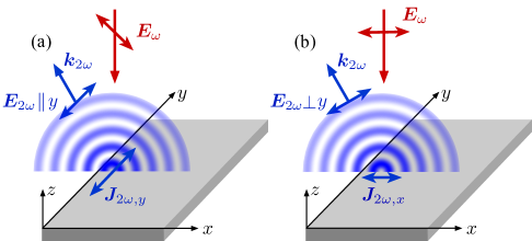
Figure 1: Second harmonic generation at the edge of 2DEG. Incident electromagnetic wave with the in-plane electric field $\bm{E}_{\omega}$ oscillating at the frequency $\omega$ induces the electric current $\bm{J}_{2\omega}$ at the double frequency in a narrow strip near the edge. In turn, the edge current $\bm{J}_{2\omega}$ emits outgoing electromagnetic wave at $2\omega$ with the electric field amplitude $\bm{E}_{2\omega}$. (a) The incident field $\bm{E}_{\omega}$ with both $x$ and $y$ components induces the current along the edge $J_{2\omega,y}\propto E_{\omega,x}E_{\omega,y}$ emitting the wave with $\bm{E}_{2\omega}\parallel y$. (b) For the incident field $\bm{E}_{\omega}\parallel x$, the edge current flows perpendicular to the edge, $J_{2\omega,x}\propto E_{\omega,x}^{2}$, and the outgoing wave is polarized with $\bm{E}_{2\omega}\perp y$.

Consider a semi-infinite 2DEG occupying the half-plane $x\geq 0$ at $z=0$ and irradiated by a plane electromagnetic wave with the electric field $\bm{E}_{\omega}(t)=\bm{E}_{\omega}\mathrm{e}^{-\mathrm{i}\omega t}+\bm{E}_{\omega}^{*}\mathrm{e}^{\mathrm{i}\omega t}$, where $\bm{E}_{\omega}$ is the incident field amplitude, see Fig. 1. As we calculate below, non-linearity of the field-induced ac electron transport at the edge results in the emergence of the current oscillating at the double frequency. This current has inhomogeneous density $\bm{j}_{2\omega}(x,t)=\bm{j}_{2\omega}(x)\mathrm{e}^{-2\mathrm{i}\omega t}+\bm{j}_{2\omega}^{*}(x)\mathrm{e}^{2\mathrm{i}\omega t}$ and is localized at the edge. The direction of the edge current depends on the incident field polarization. For the field polarized perpendicularly to the edge, $\bm{E}_{\omega}\perp y$ in Fig. 1b, the current $\bm{j}_{2\omega}$ is perpendicular to the edge. The field $\bm{E}_{\omega}$ with both parallel and perpendicular components induces also the current $\bm{j}_{2\omega}$ along the edge, Fig. 1a.

The edge current, in turn, emits electromagnetic waves with the frequency $2\omega$ and the vector potential $\bm{A}_{2\omega}(\bm{r},t)=\bm{A}_{2\omega}(\bm{r})\mathrm{e}^{-2\mathrm{i}\omega t}+\bm{A}_{2\omega}^{*}(\bm{r})\mathrm{e}^{2\mathrm{i}\omega t}$. The field $\bm{A}_{2\omega}(\bm{r})$ can be found from the wave equation Landau2

$$\Delta\bm{A}_{2\omega}+k_{2\omega}^{2}\bm{A}_{2\omega}=-\frac{4\pi}{c}\bm{j}_{2\omega}(x)\delta(z)\>,$$ (1)

where $k_{2\omega}=2\omega/c$ is the wave vector of the emitted wave and $\delta(z)$ is the Dirac delta-function. Translation invariance in the $y$ direction implies that $\bm{A}_{2\omega}$ is independent of $y$.

The Green function of the two-dimensional Helmholtz equation enables us to present the solution of Eq. (1) in the form

$$\bm{A}_{2\omega}(\bm{r})=\frac{\mathrm{i}\pi}{c}\int\bm{j}_{2\omega}(x^{\prime})\mathrm{H}_{0}^{(1)}\left(k_{2\omega}\sqrt{(x-x^{\prime})^{2}+z^{2}}\right)dx^{\prime},$$ (2)

where $\mathrm{H}_{0}^{(1)}$ is the Hankel function of the first kind.

Far from the edge, $\bm{A}_{2\omega}(\bm{r})$ represents the outgoing cylindrical wave. Its parameters can be found by analyzing the asymptotic of $\bm{A}_{2\omega}(\bm{r})$ at large $R=\sqrt{x^{2}+z^{2}}$. The asymptotic expansion of the Hankel function at large arguments has the form $\mathrm{H}_{0}^{(1)}(\xi)\approx\sqrt{2/(\pi\xi})\exp(\mathrm{i}\xi-\mathrm{i}\pi/4)$. Then, in the far field zone, i.e., at $R\gg 2\pi/k_{2\omega}$, and in the dipole approximation Landau2 , which suggests $k_{2\omega}l\ll 2\pi$, where $l$ is the width of the stripe where the edge current flows, the field is given by

$$\bm{A}_{2\omega}(\bm{r})=\frac{\mathrm{i}\sqrt{2\pi}}{c\sqrt{k_{2\omega}R}}\exp\left[\mathrm{i}\left(k_{2\omega}R-\frac{\pi}{4}\right)\right]\bm{J}_{2\omega}\>,$$ (3)

where

$$\bm{J}_{2\omega}=\int_{0}^{+\infty}\bm{j}_{2\omega}(x)dx$$ (4)

is the total electric current at $2\omega$ flowing at the edge.

The magnetic and electric fields of the outgoing wave are related to the vector potential as

$$\bm{H}_{2\omega}=\mathrm{i}\bm{k}_{2\omega}\times\bm{A}_{2\omega}\>,~{}~{}~{}\bm{E}_{2\omega}=\bm{H}_{2\omega}\times\frac{\bm{k}_{2\omega}}{k_{2\omega}}\,,$$ (5)

where $\bm{k}_{2\omega}=(x/R,0,z/R)k_{2\omega}$. The current $\bm{J}_{2\omega}$ flowing along the edge emits the electromagnetic waves with the field $\bm{E}_{2\omega}$ parallel to the edge, whereas the edge current flowing perpendicularly to the edge induces the wave with the field $\bm{E}_{2\omega}$ lying in the $(x,z)$ plane, see Fig. 1.

III Kinetic theory

Now we calculate the edge current $\bm{J}_{2\omega}$. In the kinetic approach, the response of an electron system to an external field is described by the Boltzmann equation for the electron distribution function $f$. In our case $f=f(\bm{p},x,t)$, and the Boltzmann equation has the form Candussio2020 ; Durnev_pssb2021

$$\frac{\partial f}{\partial t}+v_{x}\frac{\partial f}{\partial x}+e\bm{\mathcal{E}}\cdot\frac{\partial f}{\partial\bm{p}}=\mathrm{St}f\>,$$ (6)

where $\bm{p}$ is the electron momentum, $\bm{v}=\bm{p}/m$ is the electron velocity, $m$ is the effective mass, $\bm{\mathcal{E}}(x,t)$ is the total electric field in the 2D layer acting on electrons, and $\mathrm{St}f$ is the collision integral. The collision integral describes the relaxation of electrons in the bulk of 2D layer. Additionally, we assume that electrons are reflected specularly at the edge, which implies the boundary condition $f(p_{x},p_{y},x=0)=f(-p_{x},p_{y},x=0)$.

The field $\bm{\mathcal{E}}(x,t)$ is the sum of the incident field $\bm{E}_{\omega}(t)$ and the field induced by oscillating electric charge near the edge Volkov1988

$$\mathcal{E}_{x}(x,t)=E_{\omega,x}(t)+\int\limits_{0}^{+\infty}\frac{2\rho(x^{\prime},t)dx^{\prime}}{x-x^{\prime}}\>,~{}~{}\mathcal{E}_{y}(t)=E_{\omega,y}(t)\>,$$ (7)

where $\rho(x,t)$ is the charge density given by $\rho(x,t)=e\nu\sum_{\bm{p}}(f-f_{0})$, $\nu$ is the factor of spin and valley degeneracy, $f_{0}$ is the equilibrium distribution function, and the principal value of the integral in Eq. (7) is calculated. The charge density depends on the $x$ coordinate only, therefore the $y$ component of the electric field remains unscreened. Note, that we neglect electromagnetic retardation assuming that $\sigma_{0}/{2\pi}\ll c$, where $\sigma_{0}$ is the two-dimensional conductivity of the electron gas Volkov1988 ; Zagorodnev2021 . In fact, the same inequality justifies the dipole approximation used in Eq. (3).

Since the external field is harmonic, we solve Eqs. (6) and (7) by expanding the distribution function $f$ and the electric field $\bm{\mathcal{E}}$ in the Fourier series as follows

$$f(\bm{p},x,t)=f_{0}+[f_{1}(\bm{p},x)\mathrm{e}^{-\mathrm{i}\omega t}+\mathrm{c.c.}]+[f_{2}(\bm{p},x)\mathrm{e}^{-2\mathrm{i}\omega t}+\mathrm{c.c.}]\>,$$

$$\bm{\mathcal{E}}(x,t)=[\bm{\mathcal{E}}_{\omega}(x)\mathrm{e}^{-\mathrm{i}\omega t}+\mathrm{c.c.}]+[\bm{\mathcal{E}}_{2\omega}(x)\mathrm{e}^{-2\mathrm{i}\omega t}+\mathrm{c.c.}]\>,$$ (8)

where $f_{1},\mathcal{E}_{\omega}\propto E_{\omega}$ and $f_{2},\mathcal{E}_{2\omega}\propto E_{\omega}^{2}$ in the lowest order in the incident field amplitude. Note, that $f(\bm{p},x,t)$ [as well as $\mathcal{E}_{x}(x,t)$] also contains time-independent non-equilibrium corrections $\propto E_{\omega}^{2}$. These corrections determine static edge polarization and dc edge currents Candussio2020 ; Durnev_pssb2021 . However, they are not relevant for SHG and are omitted.

Equations for the corrections $f_{1}$ and $f_{2}$ read

$$-\mathrm{i}\omega f_{1}+v_{x}\frac{\partial f_{1}}{\partial x}+e\bm{{\cal E}}_{\omega}\cdot\frac{\partial f_{0}}{\partial\bm{p}}=\mathrm{St}f_{1}\>,$$ (9)

$$-2\mathrm{i}\omega f_{2}+v_{x}\frac{\partial f_{2}}{\partial x}+e\bm{{\cal E}}_{\omega}\cdot\frac{\partial f_{1}}{\partial\bm{p}}+e\bm{{\cal E}}_{2\omega}\cdot\frac{\partial f_{0}}{\partial\bm{p}}=\mathrm{St}f_{2}\>,$$ (10)

where

$$\mathcal{E}_{n\omega,x}(x)=E_{\omega,x}\delta_{n,1}+\int\limits_{0}^{+\infty}\frac{2\rho_{n\omega}(x^{\prime})dx^{\prime}}{x-x^{\prime}}\,,$$ (11)

$\mathcal{E}_{n\omega,y}=E_{\omega,y}\delta_{n,1}$, and $\rho_{n\omega}(x)=e\nu\sum_{\bm{p}}f_{n}(\bm{p},x)$.

The amplitude of the local current density oscillating at $2\omega$ is determined by the correction $f_{2}$ as follows

$$\bm{j}_{2\omega}(x)=e\nu\sum\limits_{\bm{p}}\bm{v}f_{2}(\bm{p},x)$$ (12)

and the total current is given by Eq. (4). Below we solve Eqs. (9)-(11) and calculate the current components parallel and perpendicular to the edge.

IV Current along the edge

Consider first the $y$ component of the edge current. Multiplying Eq. (10) by $v_{y}$ and summing up over $\bm{p}$ we obtain

$$\sum_{\bm{p}}v_{x}v_{y}\frac{\partial f_{2}}{\partial x}+e\sum_{\bm{p}}v_{y}\left(\mathcal{E}_{\omega,x}\frac{\partial f_{1}}{\partial p_{x}}+E_{\omega,y}\frac{\partial f_{1}}{\partial p_{y}}\right)$$

$$+e\sum_{\bm{p}}v_{y}\mathcal{E}_{2\omega,x}\frac{\partial f_{0}}{\partial p_{x}}=(2\mathrm{i}\omega-\tau_{1}^{-1})\sum_{\bm{p}}v_{y}f_{2}\>,$$ (13)

where $\tau_{1}$ is the momentum relaxation time defined as $\sum_{\bm{p}}v_{\alpha}\mathrm{St}f=-\tau_{1}^{-1}\sum_{\bm{p}}v_{\alpha}f$. Taking into account that $\sum_{\bm{p}}v_{y}\partial f_{n}/\partial p_{x}=0$ and $\sum_{\bm{p}}v_{y}\partial f_{n}/\partial p_{y}=-(1/m)\sum_{\bm{p}}f_{n}$ we obtain the current density

$$j_{2\omega,y}=-\frac{e\nu\tau_{1}}{1-2\mathrm{i}\omega\tau_{1}}\left[\sum\limits_{\bm{p}}v_{x}v_{y}\frac{\partial f_{2}}{\partial x}-\frac{eE_{\omega,y}}{m}\sum\limits_{\bm{p}}f_{1}\right]\>.$$ (14)

The total current $J_{2\omega,y}$ given by Eq. (4) is found by integrating Eq. (14) over $x$. Using the relation $\sum_{\bm{p}}f_{1}=-(\mathrm{i}/\omega)\sum_{\bm{p}}v_{x}\partial f_{1}/\partial x$, which follows from Eq. (9), we obtain

$$J_{2\omega,y}=-\frac{e\nu\tau_{1}}{1-2\mathrm{i}\omega\tau_{1}}\sum\limits_{\bm{p}}v_{x}v_{y}\left[f_{2}(\bm{p},+\infty)-f_{2}(\bm{p},0)\right]\\ -\frac{\mathrm{i}e^{2}\nu\tau_{1}E_{\omega,y}}{m\omega(1-2\mathrm{i}\omega\tau_{1})}\sum\limits_{\bm{p}}v_{x}\left[f_{1}(\bm{p},+\infty)-f_{1}(\bm{p},0)\right]\>.$$ (15)

Equation (15) is general and does not rely on particular type of boundary conditions. It shows that the current at $2\omega$ emerges if the field-induced corrections to the electron distribution at the edge and the 2D bulk are different.

To proceed further, we note that $\sum_{\bm{p}}v_{x}f_{1}(\bm{p},0)=0$ since the current through the edge does not flow. The sum $\sum_{\bm{p}}v_{x}v_{y}f_{2}(\bm{p},0)$ also vanishes for the specular reflection of electrons from the edge. Therefore, the edge current $J_{2\omega,y}$ is determined by the corrections to the distribution function far from the edge, where the electric field is unscreened, i.e. $\bm{\mathcal{E}}_{\omega}=\bm{E}_{\omega}$ and $\bm{\mathcal{E}}_{2\omega}=0$, and the electron distribution is homogeneous.

The term $\sum_{\bm{p}}v_{x}f_{1}(\bm{p},+\infty)$ describes ac electric current and can be expressed via the bulk conductivity as follows

$$e\nu\sum_{\bm{p}}\bm{v}f_{1}(\bm{p},+\infty)=\sigma_{\omega}\bm{E}_{\omega}\>,$$ (16)

where $\sigma_{\omega}=\sigma_{0}/(1-\mathrm{i}\omega\tau_{1})$ is the conductivity at frequency $\omega$, $\sigma_{0}=n_{e}e^{2}\tau_{1}/m$ is the static conductivity, and $n_{e}$ is the carrier density. The term $\sum_{\bm{p}}v_{x}v_{y}f_{2}(\bm{p},+\infty)$ is calculated by multiplying Eq. (10) by $v_{x}v_{y}$ and summing up the result over $\bm{p}$, which gives

$$\sum\limits_{\bm{p}}v_{x}v_{y}f_{2}(\bm{p},+\infty)=\frac{e\tau_{2}}{m(1-2\mathrm{i}\omega\tau_{2})}\\ \times\sum_{\bm{p}}f_{1}(\bm{p},+\infty)\left(v_{x}E_{\omega,y}+v_{y}E_{\omega,x}\right),$$ (17)

where $\tau_{2}$ is the relaxation time of the second angular harmonic, $1/\tau_{2}=-\sum_{\bm{p}}v_{x}v_{y}\mathrm{St}f/\sum_{\bm{p}}v_{x}v_{y}f$.

Finally, taking into account Eqs. (15), (16), and (17), we obtain the current along the edge

$$J_{2\omega,y}=-\frac{\mathrm{i}e\sigma_{0}\tau_{1}(1-4\mathrm{i}\omega\tau_{2})}{m\omega(1-\mathrm{i}\omega\tau_{1})(1-2\mathrm{i}\omega\tau_{1})(1-2\mathrm{i}\omega\tau_{2})}E_{\omega,x}E_{\omega,y}\>.$$ (18)

The current $J_{2\omega,y}$ is proportional to $E_{\omega,x}E_{\omega,y}$. It reaches maxima for the field $\bm{E}_{\omega}$ linearly polarized at the angle $\pm\pi/4$ with respect to the edge and for circularly polarized field. The current vanishes for the field $\bm{E}_{\omega}$ polarized along or perpendicular to the edge.

Figure 2 shows the frequency dependence of the current $J_{2\omega,y}$. The current is calculated after Eq. (18) for linearly polarized incident field $\bm{E}_{\omega}$ and different ratio between the relaxation times $\tau_{2}$ and $\tau_{1}$. Since $J_{2\omega,y}$ is complex, both the modulus and the argument of $J_{2\omega,y}$ are plotted. We consider two cases: $\tau_{2}=\tau_{1}$, which corresponds to electron scattering by short-range impurities, and $\tau_{2}\ll\tau_{1}$, which corresponds to the hydrodynamic regime when frequent electron-electron collisions destroy the second angular harmonic of the distribution function. In the latter case, the first contribution to the edge current in Eq. (15) vanishes. Figure 2 shows that $J_{2\omega,y}$ is weakly sensitive to the $\tau_{2}/\tau_{1}$ ratio. The current $\propto 1/\omega$ and $\propto 1/\omega^{3}$ at low and high frequencies, respectively.

Figure 2: Frequency dependence of the edge current at $2\omega$ flowing parallel to the edge. The dashed line corresponds to short-range scattering with $\tau_{1}=\tau_{2}$, the solid line stands for the hydrodynamic regime with $\tau_{2}\ll\tau_{1}$. The main graph and the inset show the modulus $|J_{2\omega,y}|$ and the argument $\mathrm{arg}(J_{2\omega,y})$ of the complex-value current $J_{2\omega,y}$, respectively. The current is measured in $J_{0}=2e\sigma_{0}\tau_{1}^{2}E_{\omega,x}E_{\omega,y}/m$.

Figure 3 shows the spatial distributions of the current density $j_{2\omega,y}(x)$ near the edge. Different curves correspond to different $\omega\tau_{1}$. The distributions are obtained from Eq. (14) for $\tau_{2}\ll\tau_{1}$, when the first term in Eq. (14) is negligible. The second term is then found by numerical calculations of the charge density $\rho_{\omega}(x)=e\nu\sum_{\bm{p}}f_{1}$ in the local response approximation (see next section for details). In this approximation, the decay of the edge current $j_{2\omega,y}(x)$ in the 2D bulk is determined by the length of dynamical screening $l_{\rm scr}=\sigma_{0}/\omega$. Hence, the current profile narrows with the frequency increase. At large $\omega\tau_{1}$, $\mathrm{arg}(j_{2\omega,y})$ exhibits spatial oscillations, i.e., the currents $j_{2\omega,y}$ at different $x$ are phase-shifted and flow in the opposite directions in the nearby regions. These oscillations are caused by excitation of the edge plasmons, see App. A for details.

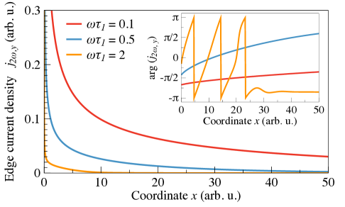
Figure 3: Spatial profile of the edge current density $j_{2\omega,y}(x)$ induced by linearly polarized field $E_{\omega,x}=E_{\omega,y}$. The main graph and the inset show the modulus $|j_{2\omega,y}|$ and the argument $\mathrm{arg}(j_{2\omega,y})$ of the complex-value current $j_{2\omega,y}$, respectively. The current density is calculated numerically in the local response approximation.

V Current normal to the edge

Now consider the $x$ component of the edge current. Multiplying Eq. (10) by $v_{x}$, summing up over $\bm{p}$, and taking into account that $\sum_{\bm{p}}v_{x}\partial f_{1}/\partial p_{y}=0$ and $\sum_{\bm{p}}v_{x}\partial f_{n}/\partial p_{x}=-(1/m)\sum_{\bm{p}}f_{n}$, we obtain

$$j_{2\omega,x}=\frac{-e\nu\tau_{1}}{1-2\mathrm{i}\omega\tau_{1}}\left[\sum\limits_{\bm{p}}v_{x}^{2}\frac{\partial f_{2}}{\partial x}-\frac{e\mathcal{E}_{\omega,x}}{m}\sum\limits_{\bm{p}}f_{1}\right]+\sigma_{2\omega}\mathcal{E}_{2\omega,x}\>,$$ (19)

where $\sigma_{2\omega}=\sigma_{0}/(1-2\mathrm{i}\omega\tau_{1})$ is the conductivity at double frequency.

The total current is obtained from Eq. (19) by integrating over $x$. Using the relation $\sum_{\bm{p}}f_{1}=-(\mathrm{i}/\omega)\sum_{\bm{p}}v_{x}\partial f_{1}/\partial x$, we obtain

$$J_{2\omega,x}=-\frac{e\nu\tau_{1}}{1-2\mathrm{i}\omega\tau_{1}}\sum\limits_{\bm{p}}v_{x}^{2}\left[f_{2}(\bm{p},+\infty)-f_{2}(\bm{p},0)\right]\\ -\frac{\mathrm{i}e^{2}\nu\tau_{1}E_{\omega,x}}{m\omega(1-2\mathrm{i}\omega\tau_{1})}\sum\limits_{\bm{p}}v_{x}[f_{1}(\bm{p},+\infty)-f_{1}(\bm{p},0)]\\ +\frac{\mathrm{i}e^{2}\nu\tau_{1}}{m\omega(1-2\mathrm{i}\omega\tau_{1})}\int\frac{d{\cal E}_{\omega,x}}{dx}\sum\limits_{\bm{p}}\ v_{x}f_{1}\,dx+\sigma_{2\omega}\int\mathcal{E}_{2\omega,x}(x)dx\>.$$ (20)

Comparing Eqs. (15) and (20) one observes that the current perpendicular to the edge contains two additional contributions which are not proportional to a difference between the distribution function at the edge and in the 2D bulk. Evaluation of these terms requires the knowledge of the distribution function corrections $f_{1}$ and $f_{2}$ and the electric field $\mathcal{E}_{x}$ in the whole half-space $x>0$. The corrections and the field can be found numerically from Eqs. (9)-(11). However, solving Eqs. (9)-(11) self-consistently is, in general, a challenging task. Therefore, in what follows we consider two approximations.

Note that symmetry consideration of the edge SHG allows the current $J_{2\omega,x}$ to be induced by $E_{\omega,x}^{2}$ and $E_{\omega,y}^{2}$. However, the analysis of Eqs. (19), (9), and (10) shows that, for specular reflection of electrons from the edge, $J_{2\omega,x}\propto E_{\omega,x}^{2}$, i.e., the current $J_{2\omega,x}$ vanishes for the field $\bm{E}_{\omega}$ polarized along the edge. This result also holds in the local response approximation considered below.

V.1 Strong screening. Local response approximation

In the absence of high-$\varepsilon$ dielectric environment, Coulomb interaction in 2D systems is dominant and, therefore, drift currents induced by local electric fields prevail over diffusion currents. In the local response approximation Mikhailov2005 , terms with the spatial gradients in equations for the current density are neglected. As a result, equations for the current density at $\omega$ and $2\omega$ assume the form

$$j_{\omega,x}(x)=\sigma_{\omega}\mathcal{E}_{\omega,x}(x)\>$$ (21)

and

$$j_{2\omega,x}(x)=\frac{e\tau_{1}\rho_{\omega}(x)\mathcal{E}_{\omega,x}(x)}{m(1-2\mathrm{i}\omega\tau_{1})}+\sigma_{2\omega}\mathcal{E}_{2\omega,x}(x)\>.$$ (22)

The latter follows directly from Eq. (19).

To find the spatial profile of the current density $j_{2\omega,x}(x)$ and the total current $J_{2\omega,x}$ we solve Eqs. (21) and  (22) self-consistently with Eqs. (11) for $\mathcal{E}_{n\omega,x}(x)$ and the continuity equations $-\mathrm{i}n\omega\rho_{n\omega}+dj_{n\omega,x}/dx=0$, see Appendix A for details. The absence of the current through the edge implies the boundary conditions $j_{n\omega,x}(0)=0$.

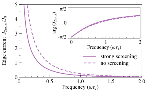
Figure 4: Frequency dependence of the edge current at $2\omega$ flowing perpendicular to the edge. The solid line corresponds to the local response approximation in the regime of strong screening. The dashed line is calculated in the hydrodynamic regime with $\tau_{2}\ll\tau_{1}$ and neglecting screening. The main graph and the inset show the modulus $|J_{2\omega,x}|$ and the argument $\mathrm{arg}(J_{2\omega,x})$ of the complex-value current $J_{2\omega,x}$, respectively. The current is measured in $J_{0}=e\sigma_{0}\tau_{1}^{2}E_{\omega,x}^{2}/m$.

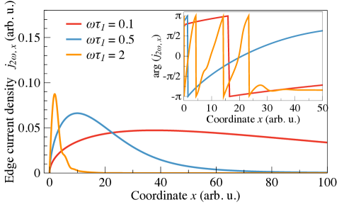
Figure 5: Spatial profile of the edge current density $j_{2\omega,x}(x)$ induced by linearly polarized field $\bm{E}_{\omega}\parallel x$. The main graph and the inset show the modulus $|j_{2\omega,x}|$ and the argument $\mathrm{arg}(j_{2\omega,x})$ of the complex-value current $j_{2\omega,x}$, respectively. The current density is calculated numerically in the local response approximation, Eq. (22).

Figure 4 shows the frequency dependence of the current $J_{2\omega,x}$. The solid line shows the current calculated numerically in the local response approximation for linearly polarized incident field $\bm{E}_{\omega}\parallel x$. The dependence closely follows the one for $J_{2\omega,y}$ shown in Fig. 2, and the phase shift between $J_{2\omega,x}$ and $J_{2\omega,y}$ for linearly polarized incident field is close to zero.

Figure 5 shows the spatial distributions of the current density $j_{2\omega,x}(x)$ near the edge. Different curves correspond to different $\omega\tau_{1}$. Similarly to the current along the edge $j_{2\omega,y}$, the current $j_{2\omega,x}$ decays in the 2D bulk on the scale of the screening length $l_{\rm scr}=\sigma_{0}/\omega$ and its profile narrows with the frequency increase. In contrast to $j_{2\omega,y}$, the current $j_{2\omega,x}$ vanishes at $x=0$ as set by boundary conditions. Similarly to $j_{2\omega,y}$, the profile of $j_{2\omega,x}$ exhibits spatial oscillations at large $\omega\tau_{1}$ caused by the excitation of edge plasmons.

V.2 Negligible screening

The opposite case of weak screening is realized if the 2D layer is surrounded by a high-$\varepsilon$ dielectric medium and one can neglect the back action of an in-plane electric field produced by charge oscillations. In this case, the total electric field $\bm{\mathcal{E}}$ acting upon the electrons coincides with the incident field $\bm{E}_{\omega}$ and the last line in Eq. (20) vanishes. To calculate the other contributions to $J_{2\omega,x}$ we need to find the difference between the distribution functions at the edge and in the bulk by solving Eqs. (9) and (10) with ${\mathcal{E}}_{\omega,x}=E_{\omega}$, ${\mathcal{E}}_{\omega,y}=0$, and $\bm{\mathcal{E}}_{2\omega}=0$. We do it analytically for $\tau_{2}\ll\tau_{1}$, which corresponds to the hydrodynamic regime of electron flow, and $\omega\tau_{2}\ll 1$. In this regime, one can retain only the zeroth and first angular harmonics in the distribution function corrections $f_{1}$ and $f_{2}$.

The functions $f_{n}(\bm{p},x)$ ($n=1,2$) can be searched in the form $f_{n}(\bm{p},x)=a_{n}(p,x)+v_{x}b_{n}(p,x)$. The absence of the current through the edge, the current at $2\omega$ in the bulk, and the charge/energy oscillations at $\omega$ in the bulk implies $b_{n}(p,0)=0$, $b_{2}(p,+\infty)=0$, and $a_{1}(p,+\infty)=0$, respectively. Solution of Eq. (9) with these boundary conditions has the form

$$a_{1}=e\lambda_{\omega}^{-1}E_{\omega,x}f_{0}^{\prime}\mathrm{e}^{-\lambda_{\omega}x},\;b_{1}=-e\tau_{\omega}E_{\omega,x}f_{0}^{\prime}\left(1-\mathrm{e}^{-\lambda_{\omega}x}\right),$$ (23)

where

$$\tau_{\omega}=\frac{\tau_{1}}{1-\mathrm{i}\omega\tau_{1}}\>,\;\;\lambda_{\omega}=(1-\mathrm{i})\sqrt{\frac{m\omega}{2\varepsilon\tau_{\omega}}}\>,$$ (24)

$\varepsilon=p^{2}/2m$, and $(...)^{\prime}=\partial(...)/\partial\varepsilon$. Equation (10) leads to the system of coupled differential equations

$$-2\mathrm{i}m\omega a_{2}+\varepsilon\frac{\partial b_{2}}{\partial x} = -eE_{\omega,x}(b_{1}\varepsilon)^{\prime},$$

$$\frac{\partial a_{2}}{\partial x}+(\tau_{1}^{-1}-2\mathrm{i}\omega)b_{2} = -eE_{\omega,x}a_{1}^{\prime}\>.$$ (25)

Its solution has the form

$$a_{2} = A+B\mathrm{e}^{-\lambda_{\omega}x}+Cx\mathrm{e}^{-\lambda_{\omega}x}-D\mathrm{e}^{-\lambda_{2\omega}x}/(\lambda_{2\omega}\tau_{2\omega})\>,$$

$$b_{2} = D\left(\mathrm{e}^{-\lambda_{\omega}x}-\mathrm{e}^{-\lambda_{2\omega}x}\right)+Fx\mathrm{e}^{-\lambda_{\omega}x}\>,$$ (26)

where $\tau_{2\omega}$ and $\lambda_{2\omega}$ are given by Eq. (24) with $\omega\to 2\omega$, and the constants $A$, $B$, $C$, $D$, $F$ are found from Eq. (V.2).

Further, we note that

$$e\nu\sum_{\bm{p}}v_{x}f_{1}(\bm{p},+\infty)=\sigma_{\omega}E_{\omega,x}\>,~{}\sum_{\bm{p}}v_{x}f_{1}(\bm{p},0)=0\>,$$

and

$$\sum_{\bm{p}}v_{x}^{2}[f_{2}(\bm{p},+\infty)-f_{2}(\bm{p},0)]=\frac{1}{2m}\sum_{\bm{p}}\varepsilon[a_{2}(p,+\infty)-a_{2}(p,0)]\,.$$

By solving Eq. (V.2) we find

$$\sum_{\bm{p}}\varepsilon[a_{2}(p,+\infty)-a_{2}(p,0)]=\frac{\mathrm{i}\sigma_{\omega}E_{\omega,x}^{2}}{\nu\,\omega}\\ \times\frac{2\tau_{\omega}^{2}+4\tau_{2\omega}\tau_{\omega}-\tau_{2\omega}^{2}+(3/4)\sqrt{2\tau_{\omega}}\sqrt{\tau_{2\omega}}(\tau_{2\omega}-6\tau_{\omega})}{(\tau_{2\omega}-2\tau_{\omega})^{2}}\>,$$ (27)

where the sign of $\sqrt{\tau_{n\omega}}$ is chosen so that $\mathrm{Re}\sqrt{\tau_{n\omega}}>0$.

Finally, Eq. (20) for the current $J_{2\omega,x}$ yields

$$J_{2\omega,x}=-\frac{\mathrm{i}e\sigma_{0}\tau_{1}E_{\omega,x}^{2}}{m\omega(1-\mathrm{i}\omega\tau_{1})(1-2\mathrm{i}\omega\tau_{1})}F(\omega)\>,$$ (28)

where

$$F(\omega)=\frac{3[8\tau_{\omega}^{2}+\sqrt{2\tau_{\omega}}\sqrt{\tau_{2\omega}}(\tau_{2\omega}-6\tau_{\omega})]}{4(\tau_{2\omega}-2\tau_{\omega})^{2}}\>.$$ (29)

The frequency dependence of the current $J_{2\omega,x}$ given by Eq. (28) is shown in Fig. 4 by the dashed line. Comparing the dashed and solid lines we see that the currents at $2\omega$ calculated in the regimes of strong and negligible screening are close in magnitude.

We recall that Eq. (28) is obtained in the hydrodynamic regime with $\tau_{2}\ll\tau_{1},\omega^{-1}$. Within the same approximation, the current along the edge $J_{2\omega,y}$ is given by Eq. (18) with $\tau_{2}=0$. In this regime, the ratio $J_{2\omega,x}/J_{2\omega,y}$ is determined by the incident field polarization and the function $F(\omega)$. The absolute value of $F(\omega)$ lies in the range $0.7-0.8$ and its argument is close to zero in the whole frequency range. The latter suggests that the ac current $\bm{J}_{2\omega}$ is linearly polarized for linearly polarized field $\bm{E}_{\omega}$.

VI Summary

To summarize, we have studied theoretically second harmonic generation (SHG) emerging at the edge of a two-dimensional (2D) electron gas. It has been shown that ac in-plane electric field oscillating at frequency $\omega$ induces ac electric current at frequency $2\omega$ near the edge. The current is formed in the edge region determined by the dynamical screening of the electric field and the mean free path of electrons. The edge current $\bm{J}_{2\omega}$ has both parallel and perpendicular to the edge components, $J_{2\omega,\parallel}\propto E_{\omega,\parallel}E_{\omega,\perp}$ and $J_{2\omega,\perp}\propto E_{\omega,\perp}^{2}$, respectively, where $\bm{E}_{\omega}$ is the driving electric field amplitude. The currents $J_{2\omega,\parallel}$ and $J_{2\omega,\perp}$ emit electromagnetic fields at $2\omega$ with different polarizations and different radiation patterns. We have developed the kinetic theory of high-frequency nonlinear edge transport which takes into account the screening of the in-plane electric field by 2D electrons. The parallel current $J_{2\omega,\parallel}$ is calculated analytically in a quite general case whereas the perpendicular current $J_{2\omega,\perp}$ is calculated in the limiting cases of strong and negligible screening. At $\omega\tau_{1}>1$, where $\tau_{1}$ is the momentum relaxation time, the spatial profile of the current density contains oscillations caused by the excitation of edge plasmons. The SHG spectroscopy can be used to visualize edges and spatial inhomogeneities in doped 2D materials and heterostructures.

Appendix A Profiles of electric field, charge, and current in the local response approximation

Here, we calculate the spatial distributions of the electric field, charge, and electric current at the edge of a 2D electron gas in the local response approximation. To this end, we solve Eqs. (11), (21), and (22) together with the continuity equations

$$-\mathrm{i}n\omega\rho_{n\omega}+\frac{dj_{n\omega,x}}{dx}=0$$ (30)

inside a strip of the width $2a$ occupying $-a\leq x\leq a$.

Equation (11) for the strip assumes the form

$$\mathcal{E}_{n\omega,x}(x)=E_{\omega,x}\delta_{n,1}+\int\limits_{-a}^{a}\frac{2\rho_{n\omega}(x^{\prime})dx^{\prime}}{x-x^{\prime}}\>.$$ (31)

This integral equation can be inverted to express $\rho_{n\omega}$ via $\mathcal{E}_{n\omega,x}$. Taking into account that $\rho_{n\omega}$ is infinite at $x=\pm a$ and $\int_{-a}^{a}\rho_{n\omega}(x)dx=0$, we obtain Polyanin_book

$$\rho_{n\omega}(x)=\frac{xE_{\omega,x}\delta_{n,1}}{2\pi\sqrt{a^{2}-x^{2}}}\\ -\frac{1}{2\pi^{2}}\int\limits_{-a}^{a}\frac{\sqrt{a^{2}-x^{\prime 2}}\mathcal{E}_{n\omega,x}(x^{\prime})dx^{\prime}}{\sqrt{a^{2}-x^{2}}(x-x^{\prime})}\>.$$ (32)

Note that the first term in the right-hand side of Eq. (32) at $n=1$ gives the distribution of charge density induced by the static electric field, i.e., in the limit $\omega\rightarrow 0$, when the $x$ component of the field inside the strip is completely screened so that $\mathcal{E}_{\omega,x}=0$.

Equations (30) and (32) yield

$$\frac{-\mathrm{i}}{n\omega}\frac{dj_{n\omega,x}}{dx}=\frac{xE_{\omega,x}\delta_{n,1}}{2\pi\sqrt{a^{2}-x^{2}}}\\ -\frac{1}{2\pi^{2}}\int\limits_{-a}^{a}\frac{\sqrt{a^{2}-x^{\prime 2}}\mathcal{E}_{n\omega,x}(x^{\prime})dx^{\prime}}{\sqrt{a^{2}-x^{2}}(x-x^{\prime})}\>.$$ (33)

First, we analyze the linear response and calculate the distributions $\mathcal{E}_{\omega,x}(x)$, $\rho_{\omega}(x)$, and $j_{\omega,x}(x)$. By integrating Eq. (33) from $-a$ to $x$ and using Eq. (21) together with the boundary condition $j_{\omega,x}(-a)=0$ we obtain

$$\frac{\mathrm{i}l_{\rm scr}\mathcal{E}_{\omega,x}}{1-\mathrm{i}\omega\tau_{1}}=\frac{\sqrt{a^{2}-x^{2}}E_{\omega,x}}{2\pi}\\ +\int\limits_{-a}^{x}\frac{dx^{\prime\prime}}{2\pi^{2}}\int\limits_{-a}^{a}\frac{\sqrt{a^{2}-x^{\prime 2}}\mathcal{E}_{\omega,x}(x^{\prime})dx^{\prime}}{\sqrt{a^{2}-x^{\prime\prime 2}}(x^{\prime\prime}-x^{\prime})}\>.$$ (34)

Equation (34) is simplified further by introducing the variables $\alpha$ and $\beta$ as follows: $x=a\cos\alpha$ and $x^{\prime}=a\cos\beta$. Taking into account that

$$\int\limits_{-a}^{x}\frac{dx^{\prime\prime}}{\sqrt{a^{2}-x^{\prime\prime 2}}(x^{\prime}-x^{\prime\prime})}=\frac{1}{a\sin\beta}\ln\left(\frac{\sin\frac{\alpha+\beta}{2}}{|\sin\frac{\alpha-\beta}{2}|}\right),$$ (35)

we finally obtain the integral equation for $\mathcal{E}_{\omega,x}$

$$\frac{\mathrm{i}l_{\rm scr}\mathcal{E}_{\omega,x}(\alpha)}{a(1-\mathrm{i}\omega\tau_{1})}=\frac{E_{\omega,x}\sin\alpha}{2\pi}\\ -\frac{1}{2\pi^{2}}\int\limits_{0}^{\pi}\ln\left(\frac{\sin\frac{\alpha+\theta}{2}}{|\sin\frac{\alpha-\beta}{2}|}\right)\sin\beta~{}\mathcal{E}_{\omega,x}(\beta)d\beta\>.$$ (36)

Equation (36) can be solved by decomposing the electric field $\mathcal{E}_{\omega,x}(\alpha)$ in the Fourier series

$$\mathcal{E}_{\omega,x}(\alpha)=\sum\limits_{m=1}\mathcal{E}_{\omega}^{(m)}\sin m\alpha\>.$$ (37)

The integrals in Eq. (36) are calculated analytically,

$$\int\limits_{0}^{\pi}\ln\left(\frac{\sin\frac{\alpha+\beta}{2}}{|\sin\frac{\alpha-\beta}{2}|}\right)\sin m\alpha~{}d\alpha=\frac{\pi}{m}\sin m\beta\>.$$ (38)

This procedure allows us to reduce the integral Eq. (36) to the set of linear equations

$$\frac{\mathrm{i}l_{\rm scr}\pi\mathcal{E}_{\omega}^{(m)}}{a(1-\mathrm{i}\omega\tau_{1})}+\frac{1}{\pi}\sum\limits_{m^{\prime}=1}^{\infty}\mathcal{K}_{mm^{\prime}}\mathcal{E}_{\omega}^{(m^{\prime})}=\frac{E_{\omega,x}}{2}\delta_{m,1}\>,$$ (39)

where

$$\mathcal{K}_{mm^{\prime}}=-\dfrac{2[1+(-1)^{m+m^{\prime}}]m^{\prime}}{m^{\prime 4}+(m^{2}-1)^{2}-2m^{\prime 2}(m^{2}+1)}\>.$$ (40)

The Fourier components $\mathcal{E}_{\omega}^{(m)}$ can be readily found from the numerical solution of the equation set (39).

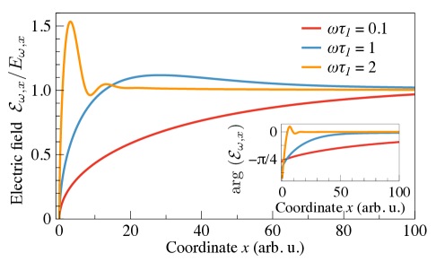
Figure 6: Spatial profiles of the electric field $\mathcal{E}_{\omega,x}(x)$ at the edge of 2D electron gas subject to the incident electric field $E_{\omega,x}$. The main graph and the inset show the modulus $|\mathcal{E}_{\omega,x}|$ and the argument $\mathrm{arg}(\mathcal{E}_{\omega,x})$ of the complex-value field $\mathcal{E}_{\omega,x}$, respectively. The field profile is calculated numerically in the local response approximation.

Figure 6 shows the spatial profiles of the electric field $\mathcal{E}_{\omega,x}(x)$ at the edge of 2D electron gas calculated after Eqs. (37), (39) for different frequencies of the incident field $E_{\omega,x}$. The $x$ coordinate in Fig. 6 is counted from the left edge of the wide strip. The calculations are done for the strip width $a\gg l_{\rm scr}$ when field profiles at the edge do not depend on $a$. Figure 6 reveals that the electric field is efficiently screened in the region $x\sim l_{\rm scr}=\sigma_{0}/\omega$ near the edge ($\mathcal{E}_{\omega,x}\sim\sqrt{x}$ at small $x$), whereas far from the edge the field is unscreened and coincides with $E_{\omega,x}$. With the frequency increase, the screening length decreases and the region of field screening narrows. At large $\omega\tau_{1}$, the profile $\mathcal{E}_{\omega,x}(x)$ contains oscillations caused by excitation of plasmons with the wave vectors $q\sim\omega^{2}/(2\pi n_{e}e^{2})=\omega\tau_{1}/(2\pi l_{\rm scr})$ Mikhailov2005 ; Zabolotnykh2019 .

Now we calculate $j_{2\omega,x}(x)$. By integrating Eq. (33) with $n=2$ over $x$ from $-a$ to $x$ and using the boundary condition $j_{2\omega,x}(-a)=0$ and Eq. (22), one obtains

$$-\frac{\mathrm{i}l_{\rm scr}j_{2\omega,x}(\alpha)}{2a(1-2\mathrm{i}\omega\tau_{1})}=\frac{1}{2\pi^{2}}\int\limits_{0}^{\pi}\ln\left(\frac{\sin\frac{\alpha+\beta}{2}}{|\sin\frac{\alpha-\beta}{2}|}\right)\sin\beta\\ \times\left[j_{2\omega,x}(\beta)-\Lambda\mathcal{E}_{\omega,x}(\beta)\frac{d\mathcal{E}_{\omega,x}}{dx}(\beta)\right]d\beta\>,$$ (41)

where

$$\Lambda=-\frac{\mathrm{i}e\sigma_{0}\tau_{1}}{m\omega(1-\mathrm{i}\omega\tau_{1})(1-2\mathrm{i}\omega\tau_{1})}$$ (42)

and $\mathcal{E}_{\omega,x}$ is the field at $\omega$ calculated above.

Decomposing the current $j_{2\omega,x}(\alpha)$ in the Fourier series,

$$j_{2\omega,x}(\alpha)=\sum\limits_{m=1}j_{2\omega}^{(m)}\sin m\alpha\>,$$ (43)

and using Eqs. (37) and (38), we reduce the integral Eq. (41) to the set of linear equations

$$\frac{\mathrm{i}l_{\rm scr}\pi j_{2\omega}^{(m)}}{2a(1-2\mathrm{i}\omega\tau_{1})}+\frac{1}{\pi^{2}}\sum\limits_{m^{\prime}=1}^{\infty}\mathcal{K}_{mm^{\prime}}j_{2\omega}^{(m^{\prime})}=\\ =-\frac{\Lambda}{4a}\left[\sum_{m^{\prime}=1}^{m-1}\frac{m^{\prime}}{m}\mathcal{E}_{\omega}^{(m^{\prime})}\mathcal{E}_{\omega}^{(m-m^{\prime})}-\sum_{m^{\prime}=m+1}^{\infty}\mathcal{E}_{\omega}^{(m^{\prime})}\mathcal{E}_{\omega}^{(m^{\prime}-m)}\right]\>.$$ (44)

The total current flowing near the left edge is found as

$$J_{2\omega,x}=\int_{-a}^{0}j_{2\omega,x}dx=a\sum_{m>1}\frac{m\cos(\pi m/2)}{m^{2}-1}j_{2\omega}^{(m)}\>.$$ (45)

The profile of the edge current calculated after Eqs. (43)-(44) is shown in Fig. 5 of the main text. The total current $J_{2\omega,x}$ is shown in Fig. 4 by the solid line.

References

• (1) E. Hendry, P. J. Hale, J. Moger, A. K. Savchenko, and S. A. Mikhailov, Coherent nonlinear optical response of graphene, Phys. Rev. Lett. 105, 097401 (2010).
• (2) M. Glazov and S. Ganichev, High-frequency electric field induced nonlinear effects in graphene, Phys. Rep. 535, 101 (2014).
• (3) M. V. Durnev and S. A. Tarasenko, High-frequency nonlinear transport and photogalvanic effects in 2D topological insulators, Ann. Phys. (Berlin) 531, 1800418 (2019).
• (4) I. A. Calafell, L. A. Rozema, D. A. Iranzo, A. Trenti, P. K. Jenke, J. D. Cox, A. Kumar, H. Bieliaiev, S. Nanot, C. Peng, D. K. Efetov, J.-Y. Hong, J. Kong, D. R. Englund, F. J. Garcia de Abajo, F. H. L. Koppens, and P. Walther, Giant enhancement of third-harmonic generation in graphene-metal heterostructures, Nat. Nanotechnol. 16, 318 (2021).
• (5) J. Zhang, W. Zhao, P. Yu, G. Yang, and Z. Liu, Second harmonic generation in 2D layered materials, 2D Mater. 7, 042002 (2020).
• (6) J. J. Dean and H. M. van Driel, Second harmonic generation from graphene and graphitic films, Appl. Phys. Lett. 95, 261910 (2009).
• (7) M. M. Glazov, Second harmonic generation in graphene, JETP Lett. 93, 366 (2011).
• (8) S. A. Mikhailov, Theory of the giant plasmon-enhanced second-harmonic generation in graphene and semiconductor two-dimensional electron systems, Phys. Rev. B 84, 045432 (2011).
• (9) Y. Wang, M. Tokman, and A. Belyanin, Second-order nonlinear optical response of graphene, Phys. Rev. B 94, 195442 (2016).
• (10) Y. Zhang, D. Huang, Y. Shan, T. Jiang, Z. Zhang, K. Liu, L. Shi, J. Cheng, J. E. Sipe, W.-T. Liu, and S. Wu, Doping-induced second-harmonic generation in centrosymmetric graphene from quadrupole response, Phys. Rev. Lett. 122, 047401 (2019).
• (11) A. Y. Bykov, T. V. Murzina, M. G. Rybin, and E. D. Obraztsova, Second harmonic generation in multilayer graphene induced by direct electric current, Phys. Rev. B 85, 121413 (2012).
• (12) L.E. Golub and S.A. Tarasenko, Valley polarization induced second harmonic generation in graphene, Phys. Rev. B 90, 201402(R) (2014).
• (13) T. O. Wehling, A. Huber, A. I. Lichtenstein, and M. I. Katsnelson, Probing of valley polarization in graphene via optical second-harmonic generation, Phys. Rev. B 91, 041404(R) (2015).
• (14) Y. W. Ho, H. G. Rosa, I. Verzhbitskiy, M. J. L. F. Rodrigues, T. Taniguchi, K. Watanabe, G. Eda, V. M. Pereira, and J. C. Viana-Gomes, Measuring valley polarization in two-dimensional materials with second-harmonic spectroscopy, ACS Photonics 7, 925 (2020).
• (15) G. Wang, X. Marie, I. Gerber, T. Amand, D. Lagarde, L. Bouet, M. Vidal, A. Balocchi, and B. Urbaszek, Giant enhancement of the optical second-harmonic emission of ${\mathrm{WSe}}_{2}$ monolayers by laser excitation at exciton resonances, Phys. Rev. Lett. 114, 097403 (2015).
• (16) E. L. Ivchenko, Optical Spectroscopy of Semiconductor Nanostructures (Alpha Science International, Oxford, UK, 2005).
• (17) S.A. Tarasenko, Direct current driven by ac electric field in quantum wells, Phys. Rev. B 83, 035313 (2011).
• (18) C. Drexler, S. A. Tarasenko, P. Olbrich, J. Karch, M. Hirmer, F. Müller, M. Gmitra, J. Fabian, R. Yakimova, S. Lara-Avila, S. Kubatkin, M. Wang, R. Vajtai, P. M. Ajayan, J. Kono, and S. D. Ganichev, Magnetic quantum ratchet effect in graphene, Nature Nanotechnol. 8, 104 (2013).
• (19) G.V. Budkin and S.A. Tarasenko, Ratchet transport of a two-dimensional electron gas at cyclotron resonance, Phys. Rev. B 93, 075306 (2016).
• (20) N. Kheirabadi, E. McCann, and V. I. Fal’ko, Cyclotron resonance of the magnetic ratchet effect and second harmonic generation in bilayer graphene, Phys. Rev. B 97, 075415 (2018).
• (21) J. Quereda, T. S. Ghiasi, J.-S. You, J. van den Brink, B. J. van Wees, and C. H. van der Wal, Symmetry regimes for circular photocurrents in monolayer MoSe2, Nat. Commun. 9, 3346 (2018).
• (22) E.L. Ivchenko and S.D. Ganichev, Spin photogalvanics, in Spin Physics in Semiconductors (second edition), ed. M.I. Dyakonov (Springer, 2018).
• (23) J. Kiemle, Ph. Zimmermann, A. W. Holleitner, and Ch. Kastl, Light-field and spin-orbit-driven currents in van der Waals materials, Nanophotonics 9, 2693 (2020).
• (24) A. Y. Bykov, P. S. Rusakov, E. D. Obraztsova, T. V. Murzina, Probing structural inhomogeneity of graphene layers via nonlinear optical scattering, Opt. Lett. 38, 4589 (2013).
• (25) Y. Li, Y. Rao, K. F. Mak, Y. You, S. Wang, C. R. Dean, and T. F. Heinz, Probing symmetry properties of few-layer MoS2 and h-BN by optical second-harmonic generation, Nano Lett. 13, 3329 (2013).
• (26) L. Mennel, M. Paur, and T. Mueller, Second harmonic generation in strained transition metal dichalcogenide monolayers: MoS2 , MoSe2, WS2, and WSe2, APL Photonics 4, 034404 (2019).
• (27) L. Zhou, H. Fu, T. Lv, C. Wang, H. Gao, D. Li, L. Deng, and W. Xiong, Nonlinear optical characterization of 2D materials, Nanomaterials 10, 2263 (2020).
• (28) E. A. Stepanov, S. V. Semin, C. R. Woods, M. Vandelli, A. V. Kimel, K. S. Novoselov, and M. I. Katsnelson, Direct observation of incommensurate – commensurate transition in graphene-hBN heterostructures via optical second harmonic generation, ACS Appl. Mater. Interfaces 12, 27758 (2020).
• (29) J. Karch, C. Drexler, P. Olbrich, M. Fehrenbacher, M. Hirmer, M. M. Glazov, S. A. Tarasenko, E. L. Ivchenko, B. Birkner, J. Eroms, D. Weiss, R. Yakimova, S. Lara-Avila, S. Kubatkin, M. Ostler, T. Seyller and S. D. Ganichev, Terahertz radiation driven chiral edge currents in graphene, Phys. Rev. Lett. 107 276601 (2011).
• (30) S. Candussio, M. V. Durnev, S. A. Tarasenko, J. Yin, J. Keil, Y. Yang, S.-K. Son, A. Mishchenko, H. Plank, V. V. Bel’kov, S. Slizovskiy, V. Fal’ko, S. D. Ganichev, Edge photocurrent driven by terahertz electric field in bilayer graphene, Phys. Rev. B 102, 045406 (2020).
• (31) S. Candussio, M. V. Durnev, S. Slizovskiy, T. Jötten, J. Keil, V. V. Bel’kov, J. Yin, Y. Yang, S.-K. Son, A. Mishchenko, V. Fal’ko, and S. D. Ganichev Edge photocurrent in bilayer graphene due to inter-Landau-level transitions, Phys. Rev. B 103, 125408 (2021).
• (32) S. Candussio, L. E. Golub, S. Bernreuter, T. Jötten, T. Rockinger, K. Watanabe, T. Taniguchi, J. Eroms, D. Weiss, and S. D. Ganichev, Nonlinear intensity dependence of edge photocurrents in graphene induced by terahertz radiation, Phys. Rev. B 104, 155404 (2021).
• (33) M. V. Durnev and S. A. Tarasenko, Rectification of ac electric current at the edge of 2D electron gas, Phys. Stat. Sol. (b) 258, 2000291 (2021).
• (34) M.V. Durnev and S.A. Tarasenko, Edge photogalvanic effect caused by optical alignment of carrier momenta in two-dimensional Dirac materials, Phys. Rev. B 103, 165411 (2021).
• (35) X. Yin, Z. Ye, D. A. Chenet, Y. Ye, K. O’Brien, J. C. Hone, and X. Zhang, Edge nonlinear optics on a MoS2 atomic monolayer, Science 344, 488 (2014).
• (36) E. D. Mishina, N. E. Sherstyuk, A. P. Shestakova, S. D. Lavrov, S. V. Semin, A. S. Sigov, A. Mitioglu, S. Anghel, and L. Kulyuk, Edge effects in second-harmonic generation in nanoscale layers of transition-metal dichalcogenides, Semicond. 49, 791 (2015).
• (37) V. A. Volkov and S. A. Mikhailov, Edge magnetoplasmons: low frequency weakly damped excitations in inhomogeneous two-dimensional electron system, Sov. Phys. JETP 67, 1639 (1988).
• (38) S. A. Mikhailov and N. A. Savostianova, Microwave response of a two-dimensional electron stripe, Phys. Rev. B 71, 035320 (2005).
• (39) A. A. Zabolotnykh and V. A. Volkov, Interaction of gated and ungated plasmons in two-dimensional electron systems, Phys. Rev. B 99, 165304 (2019).
• (40) I. V. Zagorodnev, D. A. Rodionov, and A. A. Zabolotnykh, Effect of retardation on the frequency and linewidth of plasma resonances in a two-dimensional disk of electron gas, Phys. Rev. B 103, 195431 (2021).
• (41) L. D. Landau and E. M. Lifshitz, The Classical Theory of Fields. Vol. 2, (Pergamon Press, 1977).
• (42) A. D. Polyanin, A. V. Manzhirov, Handbook of Integral Equations: Exact Solutions, (Faktorial, Moscow 1998).