The Power of Filling in Balanced Allocations

Abstract

We introduce a new class of balanced allocation processes which are primarily characterized by “filling” underloaded bins. A prototypical example is the Packing process: At each round we only take one bin sample, if the load is below the average load, then we place as many balls until the average load is reached; otherwise, we place only one ball. We prove that for any process in this class the gap between the maximum and average load is $\mathcal{O}(\log n)$ w.h.p. for any number of balls $m\geqslant 1$. For the Packing process, we also provide a matching lower bound. Additionally, we prove that the Packing process is sample-efficient in the sense that the expected number of balls allocated per sample is strictly greater than one. Finally, we also demonstrate that the upper bound of $\mathcal{O}(\log n)$ on the gap can be extended to the Memory process studied by Mitzenmacher, Prabhakar and Shah (2002).

Keywords— Balls-into-bins, balanced allocations, potential functions, heavily loaded, gap bounds, maximum load, memory, two-choices, weighted balls.
AMS MSC 2010— 68W20, 68W27, 68W40, 60C05

1 Introduction

We consider the sequential allocation of $m$ balls (jobs or data items) to $n$ bins (servers or memory cells), by allowing each ball to choose from a set of randomly sampled bins. The goal is to allocate balls efficiently, while also keeping the load distribution balanced. The balls-into-bins framework has found numerous applications in hashing, load balancing, routing, but is also closely related to more theoretical topics such as randomized rounding or pseudorandomness (we refer to the surveys [30] and [36] for more details).

A classical algorithm is the $d$-Choice process introduced by Azar, Broder, Karlin & Upfal [3] and Karp, Luby & Meyer auf der Heide [18], where for each ball to be allocated, we sample $d\geqslant 1$ bins uniformly and then place the ball in the least loaded of the $d$ sampled bins. It is well-known that for the One-Choice process ($d=1$), the gap between the maximum and average load is $\Theta\bigr{(}\sqrt{m/n\cdot\log n}\bigr{)}$ w.h.p., when $m\geqslant n\log n$. In particular, this gap grows significantly as $m\gg n$. For $d=2$, [3] proved that the gap is only $\log_{2}\log n+\mathcal{O}(1)$ w.h.p. for $m=n$. This result was generalized by Berenbrink, Czumaj, Steger & Vöcking [6] who proved that the same guarantee also holds for $m\geqslant n$, which is called the heavily loaded case. This means that the gap between the maximum and average load remains a slowly growing function in $n$ that is independent of $m$. This dramatic improvement of Two-Choice over One-Choice is widely known as the “power of two choices”.

It is natural to investigate allocation processes that are less powerful than Two-Choice in their ability to sample two bins, sample uniformly or distinguish between the load of the sampled bins. Such processes make fewer assumptions than Two-Choice and can thus be regarded as more sample-efficient and robust. As noted in [24], communication is a shortcoming of Two-Choice in some real-word systems:

More importantly, the [Two-Choice] algorithm requires communication between dispatchers and processors at the time of job assignment. The communication time is on the critical path, hence contributes to the increase in response time. (1.1)

One example of such an allocation process is the $(1+\beta)$-process analyzed by Peres, Talwar & Wieder [32], where each ball is allocated using One-Choice with probability $1-\beta$ and otherwise is allocated using Two-Choice. The authors proved that for any $\beta\in(0,1]$, the gap is $\mathcal{O}\big{(}\frac{\log n}{\beta}+\frac{\log(1/\beta)}{\beta}\big{)}$ w.h.p.; thus for any $\beta=\Omega(\operatorname{poly}(1/n))$, the gap is $\mathcal{O}\big{(}\frac{\log n}{\beta}\big{)}$. Hence, only a “small” fraction of Two-Choice rounds are enough to inherit the property of Two-Choice that the gap is independent of $m$. A similar class of adaptive sampling schemes (where, depending on the loads of the samples so far, the ball may or may not sample another bin) was analyzed by Czumaj and Stemann [9], but their results hold only for $m=n$.

Another important process is Two-Thinning, which was studied in [17, 12]. In this process, each ball first samples a bin uniformly and based on some criterion (e.g., a threshold on the load) decides whether to allocate the ball there or not. If not, the ball is placed into a second bin sample, without inspecting its load. In [12], the authors proved that for $m=n$, there is a Two-Thinning process which achieves a gap of $\mathcal{O}\big{(}{\scriptstyle\sqrt{\frac{\log n}{\log\log n}}}\big{)}$ w.h.p.. A protocol is introduced and analyzed in [2] which utilizes $d$ adaptive bin samples (on average) and improves significantly on the gap bound of $d$-Choice. These results present a vast improvement over One-Choice, however the total number of samples is greater than one per ball. Similar threshold processes have been studied in queuing [11], [28, Section 5] and discrepancy theory [10]. For values of $m$ sufficiently larger than $n$, [13] and [20] prove some lower and upper bounds for a more general class of adaptive thinning protocols (here, adaptive means that the choice of the threshold may depend on the load configuration). Related to this line of research, the authors of [20] also analyze a so-called Quantile-process, which is a version of Two-Thinning where the ball is placed into a second sample only if the first bin has a load which is at least the median load.

Finally, we mention the Memory process analyzed by Mitzenmacher, Prabhakar & Shah [29], which is essentially a version of the Two-Choice process with a cache. At each round, we take a uniform bin sample but we also have access to a cache. Then the ball is placed in the least loaded of the sampled and the cached bin, and after that the cache is updated if needed. It was shown in [29] that for $m=n$, the process achieves an asymptotically better gap than Two-Choice. In this work we prove (to the best of our knowledge) the first $\mathcal{O}(\log n)$ bound on the gap in the heavily loaded case. Later, in [22], the authors of this paper improved this to the asymptotically tight $\mathcal{O}(\log\log n)$ bound. Luczak & Norris [25] analyzed the related “supermarket” model with memory, in the queuing setting.

From a more technical perspective, apart from analyzing a large class of natural allocation processes, an important question is to understand how sensitive the gap is to changes in the allocation probability vector. To this end, [32] formulated general conditions on the probability vector, which, when satisfied in all rounds, imply a small gap bound. These were then later applied not only to the $(1+\beta$)-process, but also to analyze a “graphical” allocation model where a pair of bins is sampled by picking an edge of a graph uniformly at random.

Wieder [35] studied the $d$-Choice process with an $(a,b)$-biased sampling vector $s$, meaning that the probability of sampling bin $i$ is $\frac{1}{an}\leqslant s_{i}\leqslant\frac{b}{n}$. They showed that for the $d$-Choice process there exist constants $A:=A(d),B:=B(d)$, so that for every $(a,b)$-biased sampling vector with $a<A$ and $b<B$, the process maintains the $\mathcal{O}(\log\log n)$ gap bound, otherwise, there are sampling vectors, for which the process has an $\Omega(\sqrt{\frac{m}{n}\cdot\log n})$ gap for $m\gg n$.

Several variants of balls-into-bins have been studied, including allocations on graphs [19, 4] and hypergraphs [15, 16], balls-into-bins with correlated choices [35], balls-into-bins with hash functions [7] and balls-into-bins with deletions [5, 8].

Brief Summary of Our Results

In this work, we address the shortcoming of Two-Choice observed in [24] (see the quote (1.1) above), by studying processes that can allocate more than one balls to a sampled bin. While most of the allocation processes studied before are based on a “sampling bias” towards underloaded bins, our new class consists of processes with very weak sampling requirements (e.g., uniform sampling like in One-Choice suffices). However, our class is based on a so-called “filling operation”, meaning in the most basic form means that once an undeloaded bin is found, it is filled with balls until the average load is reached. This avoids the use of a second sample (like in Two-Choice, $(1+\beta)$-process or Thinning) and also does not require the allocator to hold and compare the load of two sampled bins (like in Two-Choice or $(1+\beta)$-process). Therefore, due to the reduced sampling and communication costs, this operation seems well suited to scenarios where an allocator needs to quickly assign a large number of jobs to a set of servers.

In order to capture not only the prototypcial Packing process but also a variety of other processes, we formulate two conditions, $\mathcal{P}$ and $\mathcal{W}$, which give rise to a broader class of allocation processes with this “filling” behavior, we call these Filling processes. Very roughly, $\mathcal{P}$ stipulates that a procedure is used to sample a single bin in each round that is not more biased towards overloaded bins than the uniform distribution. Again, very roughly, $\mathcal{W}$ states that if we sample an underloaded bin then we allocate the amount of balls that would bring that bin up to the average load, however we may distribute them almost arbitrarily over the underloaded bins; otherwise, we allocate one ball.

As our first main result (3.1), we prove that if $\mathcal{P}$ and $\mathcal{W}$ both hold, then w.h.p. for any round $m$, a gap bound of $\mathcal{O}(\log n)$ follows. Note that from here on, we will generally use $m$ to denote the number of rounds, which may be different (i.e., smaller than) the number of total balls allocated. While it is easy to show that Packing meets the two conditions, some care is needed to apply the framework to Memory due to its use of the cache, which creates strong correlations between the allocation of any two consecutive balls. The ability to allocate the balls arbitrarily among underloaded bins, means that the framework directly captures versions of the Packing process augmented with simple heuristics. For example, if the bins are uniformly accessed but also locally networked, then a bin could spread the balls it receives in a round to neighboring underloaded bins.

We also show that any process satisfying $\mathcal{P}$ and $\mathcal{W}$ allocates $1+c$ balls (for some constant $c>0$) per round in expectation (3.2). A direct consequence of this is that Packing is more sample efficient than One-Choice, while still achieving an $\mathcal{O}(\log n)$ gap. This matches the gap bound of the $(1+\beta)$-process for constant $\beta\in(0,1)$, which requires strictly more than one sample per ball, demonstrating the “power of filling” in balanced allocations. We further investigate this phenomenon by analyzing two variants of Packing: $(i)$ Tight-Packing, where the filling balls are adversarially allocated to the highest underloaded bins and $(ii)$ Packing with an $(a,b)$-biased sampling vector, where the bins may be selected using a sampling vector that majorizes One-Choice. We show that in contrast to $d$-Choice, for arbitrary $a,b>1$ being functions of $n$, the gap of this process is independent of $m$.

For Packing, we also prove a matching lower bound on the gap of $\Omega(\log n)$ for any $m=\Omega(n\log n)$. Our results on the gap are summarized in Table 1.1. We note that this work first appeared as part of the conference paper [21], the results on Non-Filling processes from [21] have also subsequently been refined [23].

Process	Lightly Loaded Case $m=\mathcal{O}(n)$				Heavily Loaded Case $m\geqslant n$
	Lower Bound		Upper Bound		Lower Bound		Upper Bound
$(1+\beta)$-process with $\beta=1/2$	[14]$\qquad\quad\;\,\frac{\log n}{\log\log n}\qquad\quad\;\,$[33]				[23]$\qquad\quad\;\,\ \log n\qquad\quad\;\,$[32]
Memory	[12]$\qquad\quad\log\log n\quad\qquad$[29]				$\log\log n$	[22]	$\log n$	(Thm 3.1)
							$\log\log n$	[22]
Packing	$\frac{\log n}{\log\log n}$	(Lem 6.1)	$\frac{\log n}{\log\log n}$	(Obs 3.4)	$\log n$	(Lem 3.6)	$\log n$	(Thm 3.1)
Tight-Packing	$\frac{\log n}{\log\log n}$	(Lem 6.1)	$\frac{\log n}{\log\log n}$	(Obs 3.4)	$\frac{\log n}{\log\log n}$	(Lem 6.1)	$\log n$	(Thm 3.1)

need to keep the table separate from caption

Table 1.1: Overview of the Gap achieved (with probability at least $1-n^{-1}$ for upper bounds and at least a positive constant for lower bounds), by different allocation processes considered in this work (and others). All stated bounds hold asymptotically; upper bounds hold for all values of $m$, while lower bounds may only hold for certain values of $m$. Cells shaded in  Green  are results proved in this paper.

Proof Overview & Ideas

To prove an upper bound on the gap for Filling processes, we consider an exponential potential function $\Phi^{t}$ with parameter $\alpha>0$ (a variant of the one used in [32, 34]). This potential function considers only bins that are overloaded by at least two balls; thus it is blind to the load configuration across underloaded bins. We upper bound $\mathbf{E}\left[\,\Phi^{t+1}\,\mid\,\Phi^{t}\,\right]$ by an expression that is maximized if the process uses the uniform distribution for picking a bin (see Lemma 4.1). We then use this upper bound to deduce that: $(i)$ in many rounds, the potential drops by a factor of at least $1-\Omega(\frac{\alpha}{n})$, and $(ii)$ in other rounds, the potential increases by a factor of at most $1+\mathcal{O}(\frac{\alpha^{2}}{n})$ (see Lemma 4.2). Taking $\alpha$ sufficiently small and constructing a suitable super-martingale, we conclude that $\mathbf{E}\left[\,\Phi^{t}\,\right]=\mathcal{O}(n)$ for all rounds $t\geqslant 0$. The desired gap bound is then implied by Markov’s inequality. There are several challenges in extending the potential function approach of [32]. The conditions in [32] do not cover allocating a varying number of balls (dependent on the load distribution) in a single round, and some care is needed as in our processes the load of underloaded bins can change by more than a constant amount in each round. Additionally, for the processes considered in [32], the potential drops in expectation in each round regardless of the load configuration. However, for our processes this is not the case (see Section B of the appendix for a concrete configuration which causes the potential to increase in expectation).

Organization

In Section 2 we define some basic mathematical notation needed for our analysis and introduce some previously studied balanced allocation processes related to our work. In Section 3 we present our framework for Filling processes and state our $\mathcal{O}(\log n)$ gap bound and sample efficiency bounds for Packing. Following this we apply these general results to the Packing, Tight-Packing, and Memory processes. In Section 4, we prove an $\mathcal{O}(\log n)$ bound on the gap for Filling processes and a bespoke bound for Packing with an $(a,b)$-biased probability vector (which is not a Filling process). In Section 5 we prove the gap bound for the so-called “unfolding” of a Filling process, and then we prove that this applies to Memory. The derivation of the lower bounds is given in Section 6. Our bounds on the sample-efficiency (and a related quantity called throughput) of Filling processes are then proved in Section 7. In Section 8 we empirically compare the gaps of the different processes. Finally, in Section 9 we conclude by summarizing our main results and pointing to some open problems.

2 Notation and Preliminaries

Let $x^{t}$ denote load vector of the $n$ bins at round $t=0,1,2,\ldots$ (the state after $t$ rounds have been completed). So in particular, $x^{0}:=(0,\ldots,0)$. In many parts of the analysis, we will assume an arbitrary labeling of the $n$ bins so that their loads at round $t$ are ordered non-increasingly, i.e.,

$$x_{1}^{t}\geqslant x_{2}^{t}\geqslant\cdots\geqslant x_{n}^{t}.$$

We now give a formal definition of the classical $d$-Choice process [3, 18] for reference.

$d$-Choice Process:
Iteration: For each $t\geqslant 0$, sample $d$ bins $i_{1},\ldots,i_{d}$ with replacement, independently and uniformly. Place a ball in a bin $i_{\min}$ satisfying $x_{i_{\min}}^{t}=\min_{1\leqslant j\leqslant d}x_{i_{j}}^{t}$, breaking ties arbitrarily.

Mixing One-Choice with Two-Choice rounds at a rate $\beta$, one obtains the $(1+\beta)$-process [32]:

$(1+\beta)$-Process:
Parameter: A probability $\beta\in(0,1]$.
Iteration: For each $t\geqslant 0$, with probability $\beta$ allocate one ball via the Two-Choice process, otherwise allocate one ball via the One-Choice process.

Unlike the standard balls-into-bins processes, some of our processes may allocate more than one ball in a single round. To this end we define $W^{t}:=\sum_{i\in[n]}x_{i}^{t}$ as the total number of balls that are allocated by round $t$ (for $d$-Choice we allocate one ball per round, so $W^{t}=t$; however our processes may allocate more than one ball in each round, that is $W^{t}\geqslant t$). Formally, an allocation process satisfies that $(x_{i}^{t+1}-x_{i}^{t})\in\mathbb{N}$ for any bin $i\in[n]$ (we only add balls) and $W^{t+1}\geqslant W^{t}+1$ (we allocate at least one ball) at any round $t\geqslant 0$. For some processes, it makes sense to define $S^{t}$ as the number of bins sampled after $t$ rounds, thus for Packing we have $S^{t}=t$ for all $t\geqslant 0$.

We define the gap as $\operatorname{Gap}(t):=\max_{i\in[n]}x_{i}^{t}-\frac{W^{t}}{n}$, which is the difference between the maximum load and average load at round $t$. When referring to the gap of a specific process $P$, we write $\operatorname{Gap}_{P}(t)$ but may simply write $\operatorname{Gap}(t)$ if the process under consideration is clear from the context. Finally, we define the normalized load of a bin $i$ as:

$$y_{i}^{t}:=x_{i}^{t}-\frac{W^{t}}{n}.$$

Further, let $B_{+}^{t}:=\left\{i\in[n]\colon y_{i}^{t}\geqslant 0\right\}$ be the set of overloaded bins, and $B_{-}^{t}:=[n]\setminus B_{+}^{t}$ be the set of underloaded bins.

Similarly to [32], some of the allocation processes we study, sample a bin $i^{t}$ in each round $t$, using a probability vector $p^{t}$, where $p_{j}^{t}$ is the probability that the process samples the $j$-th most heavily loaded bin in round $t$. We denote this sampling a according $p^{t}$ by $i^{t}\in_{p^{t}}[n]$. A special case of a probability vector is the uniform vector of One-Choice, which is $p_{i}^{t}=p_{i}=\frac{1}{n}$ for all $i\in[n]$ and $t\geqslant 0$. A probability vector is called $(a,b)$-biased for $a,b\geqslant 1$ if $\frac{1}{an}\leqslant p_{i}\leqslant\frac{b}{n}$ for all $i\in[n]$. For two probability vectors $p$ and $q$ (or analogously, for two sorted load vectors), we say that $p$ majorizes $q$ if for all $1\leqslant k\leqslant n$, $\sum_{i=1}^{k}p_{i}\geqslant\sum_{i=1}^{k}q_{i}.$

We define $\mathfrak{F}^{t}$ as the filtration corresponding to the first $t$ allocations of the process (so in particular, $\mathfrak{F}^{t}$ reveals $x^{t}$ and $i^{t-1}$). In general, with high probability (w.h.p.) refers to probability of at least $1-n^{-c}$ for some constant $c>0$. For random variables $Y,Z$ we say that $Y$ is stochastically smaller than $Z$ (or equivalently, $Y$ is stochastically dominated by $Z$) if $\mathbf{Pr}\left[\,Y\geqslant x\,\right]\leqslant\mathbf{Pr}\left[\,Z\geqslant x\,\right]$ for all real $x$. Throughout the paper, we often make use of statements and inequalities which hold only for sufficiently large $n$. For simplicity, we do not state this explicitly.

3 Our Results on Filling Processes

In this section we shall present our main results. In the first subsection we present the framework for Filling processes, then state the gap bound (3.1) and finally show they are sample-efficient (3.2) under the additional assumption of sampling each bin uniformly. In Section 3.2 we introduce the Packing process, which is our prototypical example of a Filling process, and give a lower bound showing our general gap bound is essentially best possible. The Tight-Packing process is also introduced as an example of a more adversarial process that nevertheless still fits our framework, and thus also has a logarithmic gap. Finally in Section 3.3 we introduce the Memory process and a method we call “unfolding” that can extend the applicability of our gap result. In particular, although Memory is not a Filling process we show that it is an unfolding of a suitable Filling process, and thus we obtain a gap bound for Memory for a polynomial number of balls. Finally in Section 3.4 we analyze the Packing process with an $(a,b)$-biased probability vector, which is not a Filling process but highlights the power of filling, as the gap is still independent of $m$.

3.1 Filling Processes

We now formally define the main class of processes studied in this paper. Recall that $B_{-}^{t}:=\left\{i\in[n]\colon y_{i}^{t}<0\right\}$ is the set of underloaded bins after $t$ rounds have been completed.

Filling Processes:
For each round $t\geqslant 0$, we sample a bin $i=i^{t}$ and then place a certain number of balls to $i$ (or other bins). More formally:

Condition $\mathcal{P}$: For each round $t\geqslant 0$, pick an arbitrary labeling of the $n$ bins such that $y_{1}^{t}\geqslant y_{2}^{t}\geqslant\cdots\geqslant y_{n}^{t}$. Then let $i=i^{t}\in_{p^{t}}[n]$, where $p^{t}$ is any probability vector which is majorized by the uniform distribution (One-Choice).

Condition $\mathcal{W}$: For each round $t\geqslant 0$, with $i$ being the bin chosen above:

• If $y_{i}^{t}\geqslant 0$ then allocate a single ball to bin $i$.

• If $y_{i}^{t}<0$ then allocate exactly $\lceil-y_{i}^{t}\rceil+1\geqslant 2$ balls to underloaded bins such that there can be at most two bins $k_{1},k_{2}\in B_{-}^{t}$ where:

  1. $k_{1}\in B_{-}^{t}$ receives $\lceil-y_{k_{1}}^{t}\rceil+1$ balls (i.e., $x_{k_{1}}^{t+1}=\big{\lceil}\frac{W^{t}}{n}\big{\rceil}+1$),

  2. $k_{2}\in B_{-}^{t}$ receives $\lceil-y_{k_{2}}^{t}\rceil$ balls (i.e., $x_{k_{2}}^{t+1}=\big{\lceil}\frac{W^{t}}{n}\big{\rceil}$),

  3. each $j\in B_{-}^{t}\backslash\{k_{1},k_{2}\}$ receives at most $\lceil-y_{j}^{t}\rceil-1$ balls (i.e., $x_{j}^{t+1}\leqslant\big{\lceil}\frac{W^{t}}{n}\big{\rceil}-1$).

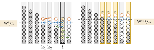
Figure 3.1: Illustration of one round for a Filling process. After the underloaded bin $i$ is picked, $\lceil-y_{i}^{t}\rceil+1=6$ balls are allocated. Only one bin $k_{1}$ receives $\lceil-y_{k_{1}}^{t}\rceil+1$ balls and only one bin $k_{2}$ receives $\lceil-y_{k_{2}}^{t}\rceil$ balls, i.e., at most one allocated bin attains a load in the orange region and at most one in the blue region. All other bins $j$ receive at most $\lceil-y_{j}^{t}\rceil-1$ balls.

See Figure 3.1 for an illustration of the effect of condition $\mathcal{W}$, if an underloaded bin is chosen.

We emphasize that in condition $\mathcal{P}$, the distribution $p^{t}$ may not only be time-dependent, but may also depend on the entire history of the process until round $t$, that is, the filtration $\mathfrak{F}^{t}$. We point out that condition $\mathcal{W}$ seems both a bit technical and arbitrary. For clarity, observe that within one round condition $\mathcal{W}$ can make at most two formerly unloaded bins overloaded; one bin by at most two balls (case $(a)$) and one bin by at most one ball (case $(b)$). This could be further relaxed (and generalized) by allowing a constant number of bins to become overloaded by a constant number of balls. However, this would come at the cost of making the analysis more tedious, while the specific choice of condition $\mathcal{W}$ already suffices to cover the processes defined later in this section.

Also, the allocation used in $\mathcal{W}$ may depend on the filtration $\mathfrak{F}^{t}$. Thus the framework also applies in the presence of an adaptive adversary, which directs all the $\lceil-y_{i}^{t}\rceil+1$ balls to be allocated in round $t$ towards the “most loaded” underloaded bins (see Tight-Packing in Section 3.2). At the other end of the spectrum, there are natural processes which have a propensity to place these balls into “less loaded” underloaded bins. One specific, more complex example is the Memory process, where due to the update of the cache after each single ball, the allocation is more skewed towards “less loaded” underloaded bins. However, as we shall discuss shortly, Memory only satisfies $\mathcal{P}$ and $\mathcal{W}$ after a suitable “folding” of rounds.

Our main result is that Filling processes have gap of order $\log n$ with high probability.

Theorem 3.1.

There exists a constant $C>0$, such that for any allocation process satisfying conditions $\mathcal{P}$ and $\mathcal{W}$, and any round $m\geqslant 1$, we have

$$\mathbf{Pr}\left[\,\operatorname{Gap}(m)\leqslant C\log n\,\right]\geqslant 1-n^{-2}.$$

This result is proven in Section 4 by analyzing a variant of the exponential potential function $\Phi$ over the overloaded bins and eventually establishing that for any $m\geqslant 1$, $\mathbf{E}\left[\,\Phi^{m}\,\right]=\mathcal{O}(n).$ Then a simple application of Markov’s inequality yields the desired result for the gap.

Recall that $W^{t}=\sum_{i\in[n]}x_{i}^{t}$ is the total number of balls allocated by round $t$. The throughput of a Filling process at round $t$ is defined as

$$\mu^{t}:=\frac{W^{t}}{t},$$

this is the average balls placed per bins sampled during the first $t$ rounds. The following theorem bounds the expected throughput for Filling processes.

Theorem 3.2.

There exist constants $c,C>0$ such that for any allocation process satisfying conditions $\mathcal{P}$ and $\mathcal{W}$ and round $m\geqslant 2$, we have

$$\mathbf{E}[\,\mu^{m}\,]\geqslant 1+c,$$

and if additionally the probability vector of the allocation process is uniform at each round (this still satisfies $\mathcal{P}$), then for any round $m\geqslant 2$,

$$1+c\leqslant\mathbf{E}[\,\mu^{m}\,]\leqslant C.$$

Further, recall that $S^{t}$ is the number of bins sampled by round $t$. We define the sample efficiency by

$$\eta^{t}=\frac{W^{t}}{S^{t}},$$

this is the average balls placed per bin sampled during the first $t$ rounds. Observe that for any $t\geqslant 1$ we have $\eta^{t}=1$ for One-Choice and $\eta^{t}=1/2$ for Two-Choice deterministically. For Packing, $S^{t}=t$ and so $\eta^{t}=\mu^{t}$. Therefore, 3.2 implies that Packing is more sample-efficient than One-Choice by a constant factor in expectation.

Corollary 3.3.

There exist constants $c,C>0$ (given by 3.2) such that for any round $m\geqslant 2$, the the Packing process satisfies

$$1+c\leqslant\mathbf{E}\left[\,\eta^{m}\,\right]\leqslant C.$$

The key idea in the proof of 3.2 is the observation that within any window of $n$ rounds, in a constant proportion of the rounds there is either a large number of underloaded bins or the absolute value potential function is linear. If the first event holds in a round, then we pick an underloaded bin with constant probability, thus conditional on this event the expected number of balls increases by more than one since we allocate at least two balls to an underloaded bin. The increase in the expected number of balls allocated conditional on the second event comes from a direct relationship between the number of balls allocated in a round and the absolute value potential.

For the lightly loaded case $m=n$, we can obtain a tighter upper bound on the gap, by observing that for a bin to have a gap of $g$ it must be chosen as an overloaded bin at least $g-2$ times. Hence, by the maximum load of One-Choice for $m=n$ (e.g., [31, Lemma 5.1]), we get:

Observation 3.4.

For any allocation process satisfying conditions $\mathcal{P}$ and $\mathcal{W}$ we have

$$\mathbf{Pr}\left[\,\operatorname{Gap}(n)\leqslant 3\cdot\frac{\log n}{\log\log n}\,\right]\geqslant 1-n^{-1}.$$

In Lemma 6.1 we prove a matching lower bound for any process which samples one bin uniformly in each round.

3.2 The Packing Process

A natural example of a process satisfying $\mathcal{P}$ and $\mathcal{W}$ is Packing, which places “greedily” as many balls as possible into an underloaded bin (i.e., a bin with load below average).

Packing Process:
Iteration: For each $t\geqslant 0$, sample a uniform bin $i$, and update its load:

$$x_{i}^{t+1}=\begin{cases}x_{i}^{t}+1&\mbox{if $x_{i}^{t}\geqslant\frac{W^{t}}{n}$},\\ \left\lceil\frac{W^{t}}{n}\right\rceil+1&\mbox{if $x_{i}^{t}<\frac{W^{t}}{n}$}.\end{cases}$$

See Figure 3.2 for an illustration of Packing. It is simple to show that this is a Filling process.

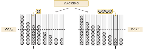
Figure 3.2: Illustration of the two different possibilities in a single round of the Packing process: (left) allocating a single ball to an overloaded bin and (right) filling an underloaded bin.

Lemma 3.5.

The Packing process satisfies conditions $\mathcal{P}$ and $\mathcal{W}$.

Proof.

The Packing process picks a uniform bin $i$ at each round $t$, thus it satisfies $\mathcal{P}$. Furthermore, if $y_{i}^{t}<0$, it allocates exactly $\lceil-y_{i}^{t}\rceil+1$ balls to bin $i$; otherwise, it allocates one ball to $i$, and thus $\mathcal{W}$ is also satisfied. ∎

The Packing process is quite similar to One-Choice in that it samples one bin per round, however, Theorem 3.1 shows that it has a $\mathcal{O}(\log n)$ gap. We also prove the following lower bound which shows that the upper bound is essentially best possible.

Theorem 3.6.

There exists a constant $\kappa>0$ such that for any $m\geqslant\kappa n\log n$ the Packing process satisfies

$$\mathbf{Pr}\left[\,\operatorname{Gap}(m)\geqslant\frac{\sqrt{\kappa}}{20}\cdot\log n\,\right]\geqslant\frac{1}{2}.$$

The Packing process arises naturally when one is trying to achieve a small gap from few bin queries or random samples. In contrast, the following process is rather contrived, as whenever an underloaded bin is chosen, balls can be placed into (possibly different) underloaded bins that have the highest load. However, it is interesting that even this process achieves a small gap, as we shall show it is a Filling process. Furthermore, experiments suggest that this process frequently leads to load configurations where the lightest bin has a normalized load of $-\omega(\log n)$. We leave it as an open problem to establish this theoretically. If this is the case then it would show that the hyperbolic cosine potential with constant smoothing parameter used in [32] cannot be used directly to deduce an $\mathcal{O}(\log n)$ gap bound for Filling processes.

Tight-Packing Process:
Iteration: For each $t\geqslant 0$, sample a uniform bin $i$, and update:

$$\left\{\!\!\!\begin{tabular}[]{ l l }$x_{i}^{t+1}=x_{i}^{t}+1$&\mbox{\phantom{shift}if $x_{i}^{t}\geqslant\frac{W^{t}}{n}$},\vspace{.25cm }\\ \text{allocate $\lceil-y_{i}^{t}\rceil+1$ balls one by one into the bins $\ell$}&\hbox{\multirowsetup\mbox{\phantom{shift}if $x_{i}^{t}<\frac{W^{t}}{n}$,}}\\ \text{with highest loads such that $x_{\ell}^{t+1}<\frac{W^{t}}{n}$, except for}&\\ \text{one bin $j$ that gets $x_{j}^{t+1}=\big{\lceil}\frac{W^{t}}{n}\big{\rceil}+1$.}&\end{tabular}\right.$$

An equivalent (and more formal) description of Tight-Packing is the following: Assume the bin loads are decreasingly sorted $x_{1}^{t}\geqslant x_{2}^{t}\geqslant\cdots\geqslant x_{n}^{t}$. If the selected bin $i\in[n]$ is overloaded, then we allocate one ball in $i$. Otherwise, we update the load of the maximally loaded underloaded bin $j\in[n]$ at round $t$ to $x_{j}^{t+1}=\big{\lceil}\frac{W^{t}}{n}\big{\rceil}+1$. Then the remaining $(\lceil-y_{i}^{t}\rceil+1)-(\lceil-y_{j}^{t}\rceil+1)=\lceil-y_{i}^{t}\rceil-\lceil-y_{j}^{t}\rceil\geqslant 0$ balls (if there are any), are allocated to bins $j+1,j+2,\ldots,j+\ell$ for some integer $\ell\geqslant 0$, such that all bins $k\in[j+1,j+\ell-1]$ have $x_{k}^{t+1}=\big{\lceil}\frac{W^{t}}{n}\big{\rceil}-1$ and $x_{j+\ell}^{t+1}\in[x_{j+\ell}^{t},\big{\lceil}\frac{W^{t}}{n}\big{\rceil})$. See Figure 3.3 for an illustration of the Tight-Packing process.

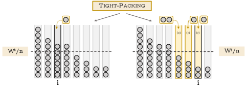
Figure 3.3: Illustration of the two different possibilities in a single round of the Tight-Packing process: (left) allocating a single ball to an overloaded bin and (right) allocating as many balls as the underload of the selected bin, to the most underloaded bins. Note that only one of the three bins where balls were allocated, attains a load of $\geqslant\lceil W^{t}/n\rceil$.

As promised we now show that this is also a Filling process.

Lemma 3.7.

The Tight-Packing process satisfies conditions $\mathcal{P}$ and $\mathcal{W}$.

Proof.

The Tight-Packing process picks a uniform bin $i$ at each round $t$, thus it satisfies $\mathcal{P}$. Further, the allocation satisfies the following properties regarding the allocation of balls.

First, in case of $y_{i}^{t}<0$, then: $(i)$ we allocate exactly $\lceil-y_{i}^{t}\rceil+1$ balls, $(ii)$ one bin receives $\lceil-y_{j}^{t}\rceil+1$ balls (satisfying $(a)$), and $(iii)$ every other bin $j$ receives a number of balls between $[0,\lceil-y_{j}^{t}\rceil-1]$ (satisfying $(c)$).

Secondly, in case of $y_{i}^{t}\geqslant 0$ we place one ball to $i$. Thus $\mathcal{W}$ is also satisfied. ∎

3.3 Memory and Unfolding

The Memory process was introduced by Mitzenmacher, Prabhakar & Shah [29] and works under the assumption that the address $b$ of a single bin can be stored or “cached”. The process is essentially a Two-Choice process where the second sample is replaced by the bin in the cache.

Memory Process:
Iteration: For each $t\geqslant 0$, sample a uniform bin $i$, and update its load (or of cached bin $b$):

$$\begin{cases}x_{i}^{t+1}=x_{i}^{t}+1&\mbox{if $x_{i}^{t}<x_{b}^{t}$}\qquad\mbox{(also update cache $b=i$)},\\ x_{i}^{t+1}=x_{i}^{t}+1&\mbox{if $x_{i}^{t}=x_{b}^{t}$},\\ x_{b}^{t+1}=x_{b}^{t}+1&\mbox{if $x_{i}^{t}>x_{b}^{t}$}.\end{cases}$$

See Figure 3.4 for an illustration of the Memory process.

As mentioned above, Memory does not satisfy conditions $\mathcal{P}$ and $\mathcal{W}$ directly. The issue is that Memory allocates only one ball at each round whereas, due to condition $\mathcal{W}$, a Filling process may place several balls into underloaded bins in a single round. To overcome this issue, we define a so-called unfolding of a Filling process. The Filling process proceeds in rounds $0,1,\ldots$, whereas the unfolding is a coupled process, which is encoded as a sequence of atomic allocations (each allocation places exactly one ball into a bin). Using this unfolding along with the gap bound for a Filling process satisfying $\mathcal{P}$ and $\mathcal{W}$, we can then bound the number of atomic allocations with a large gap.

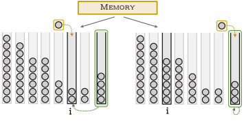
Figure 3.4: Illustration of the two different possibilities in a single round of the Memory process: (left) allocating to the sampled bin and (right) updating the cache or allocating to the cache (shown in green).

First, we define unfolding formally: Let $x^{t}$ be the load vector of a Filling process $P$, and $\widehat{x}^{\,t}$ be the load vector of the unfolding of $P$ called $U=U(P)$. Initialize $x^{0}:=\widehat{x}^{\,0}$ as the all-zero vector, corresponding to the empty load configuration. For every round $t\geqslant 1$, where $P$ has allocated $W^{t-1}$ balls in the previous rounds, we create atomic allocations $A(t):=\{W^{t-1}+1,\ldots,W^{t}\}$ for the process $U$, where $W^{t}=W^{t-1}+\min\left\{\lceil-y_{i}^{t}\rceil+1,\;1\right\}$, such that for each $s\in A(t)$ a single ball is allocated in the process $U$. Additionally, we have $x^{t}:=\widehat{x}^{\,W^{t}}$, i.e., the load distribution of $P$ after round $t$ corresponds to load distribution of $U$ after atomic allocation $W^{t}\geqslant t$. Note that the unfolding of a process is not (completely) unique, as the allocations in $[W^{t-1}+1,W^{t}]$ of $U(P)$ can be permuted arbitrarily.

The next result shows that Memory can be considered as a filling process after it has been “unfolded”.

Lemma 3.8.

There is an allocation process $P$ satisfying conditions $\mathcal{P}$ and $\mathcal{W}$, such that for a suitable unfolding $U=U(P)$, the allocation process $U$ is an instance of Memory.

Now, applying 3.1 to the unfolding of a Filling process, and exploiting that in a balanced load configuration not too many atomic allocations can be created through unfolding, we obtain the following result:

Lemma 3.9.

Fix any constant $c>0$. Then for any allocation process $P$ satisfying conditions $\mathcal{P}$ and $\mathcal{W}$, there is a constant $C=C(c)>0$ such that for any number of atomic allocations $m\geqslant 1$, with probability at least $1-n^{-2}$, any unfolding $U=U(P)$ satisfies

$$\bigl{|}\left\{t\in[m]\colon\operatorname{Gap}_{U}(t)\geqslant C\cdot\log n\right\}\bigr{|}\leqslant n^{-c}\cdot m\log m.$$

Hence for any $m$, all but a polynomially small fraction of the first $m$ atomic allocations in any unfolding of a Filling process (e.g., Memory) have a logarithmic gap. This behavior matches the one of the original Filling process, under the limitation that we cannot prove a small gap that holds for an arbitrarily large fixed atomic allocation $m$. However, if $m$ is polynomial in $n$, that is, $m\leqslant n^{c}$ for some constant $c>0$, then Lemma 3.9 implies directly that with high probability, the gap at atomic allocation $m$ (and at all atomic allocations before) is logarithmic.

We note however that for the specific case of Memory, a $\mathcal{O}(\log n)$ gap bound is not tight. Since this paper was submitted, the authors proved a $\mathcal{O}(\log\log n)$ gap bound for the Memory process which holds w.h.p. for any number $m\geqslant 1$ of balls [22].

3.4 The Packing Process with a Biased Probability Vector

Finally, we also consider the Packing process with an $(a,b)$-biased sampling vector $p$, meaning that the probability of sampling bin $i$ satisfies $\frac{1}{an}\leqslant p_{i}\leqslant\frac{b}{n}$. Such a vector could even have a bias to place towards overloaded bins. For Packing the sampling vector coincides with the probability vector, so we will refer to it as probability vector from this point forward.

Packing process with an $(a,b)$-biased probability vector $p^{t}$:
Parameter: At any step $t$, probability vector $p^{t}:=p(\mathfrak{F}^{t})$ satisfying $\frac{1}{an}\leqslant p_{i}^{t}\leqslant\frac{b}{n}$ for all $i\in[n]$.
Iteration: For each $t\geqslant 0$, sample a bin $i\in_{p}[n]$, and update its load:

$$x_{i}^{t+1}=\begin{cases}x_{i}^{t}+1&\mbox{if $x_{i}^{t}\geqslant\frac{W^{t}}{n}$},\\ \Big{\lceil}\frac{W^{t}}{n}\Big{\rceil}+1&\mbox{if $x_{i}^{t}<\frac{W^{t}}{n}$}.\end{cases}$$

Note that this process is not necessarily a Filling process as its probability vector may not be majorized by the uniform distribution. Such probability vectors may occur, for instance, if the load information is noisy or outdated. Next we show that as long as $a,b$ are functions of $n$, the Packing process has a gap bound that is independent of $m$.

Proposition 3.10.

Consider the Packing process with any $(a,b)$-biased probability vector with $a:=a(n)>1$ and $b:=b(n)>1$. Then, for any round $m\geqslant 1$, we have

$$\mathbf{E}\left[\,\Delta^{m}\,\right]\leqslant 6an^{3},$$

and hence,

$$\mathbf{Pr}\left[\,\operatorname{Gap}(m)\leqslant 6an^{4}\,\right]\geqslant 1-n^{-1}.$$

This result is very simple to prove and we do not claim that the bound is tight (as it only makes use of the lower bound on the $p_{i}$’s), however we include it as it illustrates the power of filling. In particular, in [35] it was shown that for Two-Choice for sufficiently large constants $a,b>1$ (taking $a,b=10$ suffices), there exist $(a,b)$-biased sampling distributions, for which the gap will grow at least as fast as One-Choice, that is $\operatorname{Gap}(m)=\Omega(\sqrt{\frac{m}{n}\log n})$ w.h.p. for $m\gg n$. However, the Packing process has also the power to “fill” underloaded bins, and it is this power that allows it to have a bounded gap – despite the best efforts of its unruly probability vector.

4 Upper Bounds on the Gap

In this section we prove our upper bounds on the gap. We begin in Section 4.1 by defining the exponential potential function and analyzing its behavior (depending on some other constraints). Then in Section 4.2 we use a super-martingale argument to show that the exponential potential function decreases, which eventually yields the desired gap bound in 3.1. Finally in Section 4.3 we bound the gap of the Packing with an $(a,b)$-biased probability vector, by considering the absolute value potential.

4.1 Potential Function Analysis

We consider a version of the exponential potential function $\Phi$ which only takes bins into account whose load is at least two above the average load. This is defined for any round $t\geqslant 0$ by

$$\Phi^{t}:=\Phi^{t}(\alpha):=\sum_{i:y_{i}^{t}\geqslant 2}\exp\left(\alpha\cdot y_{i}^{t}\right)=\sum_{i=1}^{n}\exp\left(\alpha\cdot y_{i}^{t}\right)\cdot\mathbf{1}_{\{y_{i}^{t}\geqslant 2\}},$$

where we recall that $y_{i}^{t}=x_{i}^{t}-\frac{W^{t}}{n}$ is the normalized load of bin $i$ at round t and $\alpha>0$ is a sufficiently small constant to be fixed later. Let $\Phi^{t}_{i}=\exp\left(\alpha\cdot y_{i}^{t}\right)\cdot\mathbf{1}_{\{y_{i}^{t}\geqslant 2\}}$ and thus $\Phi^{t}=\sum_{i=1}^{n}\Phi^{t}_{i}$. We will also use the absolute value potential: for any round $t\geqslant 0$,

$$\Delta^{t}:=\sum_{i=1}^{n}\left|y_{i}^{t}\right|.$$

The next lemma provides a useful upper bound on the expected change of $\Phi$ over one round. It establishes that to bound $\mathbf{E}[\,\Phi^{t+1}\mid\mathfrak{F}^{t}\,]$ from above, we may assume the probability vector $p^{t}$ is uniform.

Lemma 4.1.

Consider any allocation process satisfying conditions $\mathcal{P}$ and $\mathcal{W}$. Then, for $\Phi:=\Phi(\alpha)$ with any $\alpha>0$ and for any round $t\geqslant 0$,

$$\mathbf{E}[\,\Phi^{t+1}\mid\mathfrak{F}^{t}\,]\leqslant\frac{1}{n}\sum_{i=1}^{n}\Phi_{i}^{t}\cdot\left(\sum_{j\colon y_{j}^{t}<1}e^{\frac{-\alpha(\lceil-y_{j}^{t}\rceil+1)}{n}}+e^{-\frac{\alpha}{n}}\cdot(|B_{\geqslant 1}^{t}|-1)+e^{\alpha-\frac{\alpha}{n}}\right)+e^{3\alpha},$$

where $B_{\geqslant 1}^{t}$ denotes the set of bins with load at least $1$.

Proof.

Recall that the filtration $\mathfrak{F}^{t}$ reveals the load vector $x^{t}$. Throughout this proof, we consider the labeling chosen by the process in round $t$ such that $x_{1}^{t}\geqslant x_{2}^{t}\geqslant\cdots\geqslant x_{n}^{t}$ and $p^{t}$ being majorized by One-Choice (according to $\mathcal{P}$). We emphasize that for this labeling, it is quite possible that $x_{i}^{t+1}$ will not be non-increasing in $i\in[n]$.

To begin, using $\Phi_{i}^{t+1}=e^{\alpha y_{i}^{t+1}}\cdot\mathbf{1}_{\{y_{i}^{t+1}\geqslant 2\}}$, we can split $\Phi^{t+1}$ over the $n$ bins as follows,

$$\mathbf{E}\left[\,\Phi^{t+1}\,\mid\,\mathfrak{F}^{t}\,\right]=\sum_{j=1}^{n}\mathbf{E}\left[\,\Phi_{j}^{t+1}\,\mid\,\mathfrak{F}^{t}\,\right].$$

Now consider the effect of picking bin $i$ for the allocation in round $t$ to the potential $\Phi^{t+1}$. Note that bin $i$ is chosen with probability equal to $p_{i}^{t}$. Observe that if bin $i$ satisfies $y_{i}^{t}<1$, then it receives at most $\lceil-y_{i}^{t}\rceil+1$ balls in round $t$, thus $y_{i}^{t+1}\geqslant 2$ if and only if $y_{i}^{t}\geqslant 1$. Using condition $\mathcal{W}$, we distinguish between the following three cases based on how allocating to $i$ changes $\Phi_{j}^{t}$ for $j\neq i$ and for $j=i$:

Case 1.A [$y_{i}^{t}<1$, $j\neq i$, $y_{j}^{t}<1$]. We will allocate $\lceil-y_{i}^{t}\rceil+1$ many balls to bins $k$ with $y_{k}^{t}<1$ (not necessarily to $i$) subject to $\mathcal{W}$. This increases the average load by $(\lceil-y_{i}^{t}\rceil+1)/n$. Since $y_{j}^{t}<1$, $\Phi_{j}^{t}=0$. Further, by condition $\mathcal{W}$ we can increase the load of $y_{j}^{t}$ by at most $\lceil-y_{j}^{t}\rceil+1$, hence, $\Phi_{j}^{t+1}=0$. Therefore, $\Phi_{j}^{t+1}=\Phi_{j}^{t}\cdot e^{\frac{-\alpha(\lceil-y_{i}^{t}\rceil+1)}{n}}$ for $j\neq i$.

Case 1.B [$y_{i}^{t}<1$, $j\neq i$, $y_{j}^{t}\geqslant 1$]. As in Case 1a, we will allocate $\lceil-y_{i}^{t}\rceil+1$ many balls to bins $k$ with $y_{k}^{t}<1$ (not necessarily to $i$) subject to $\mathcal{W}$, which increases the average load by $(\lceil-y_{i}^{t}\rceil+1)/n$. Additionally, bin $j$ will receive no balls (by condition $\mathcal{W}$), thus $\Phi_{j}^{t+1}=\Phi_{j}^{t}\cdot e^{\frac{-\alpha(\lceil-y_{i}^{t}\rceil+1)}{n}}$ for $j\neq i$.

Case 2 [$y_{i}^{t}\geqslant 1$, $j\neq i$]. We allocate one ball to $i$, which increases the average load by $1/n$, and thus $\Phi_{j}^{t+1}=\Phi_{j}^{t}\cdot e^{-\frac{\alpha}{n}}$ for $j\neq i$, which again also holds for bins $j$ that do not contribute.

Case 3 [$j=i$]. Finally, we consider the effect on $\Phi_{i}^{t+1}$. Again if $y_{i}^{t}<1$, then $\Phi_{i}^{t}=0$ and $\Phi_{i}^{t+1}=0$. Otherwise, we have $y_{i}^{t}\geqslant 1$ and we allocate one ball to $i$, and thus

$$\Phi_{i}^{t+1}=e^{\alpha\cdot(y_{i}^{t}+1)-\frac{\alpha}{n}}\mathbf{1}_{\{y_{i}^{t+1}\geqslant 2\}}=e^{\alpha\cdot y_{i}^{t}}\mathbf{1}_{\{y_{i}^{t+1}\geqslant 2\}}\cdot e^{\alpha-\frac{\alpha}{n}}\leqslant(e^{\alpha\cdot y_{i}^{t}}\mathbf{1}_{\{y_{i}^{t}\geqslant 2\}}+e^{2\alpha})\cdot e^{\alpha-\frac{\alpha}{n}},$$

where the $+e^{2\alpha}$ is added to account for the case where $1\leqslant y_{i}^{t}<2$ and so $\Phi_{i}^{t}=0$ but $0<\Phi_{i}^{t+1}\leqslant e^{3\alpha-\alpha/n}$. Thus in this case, $\Phi_{i}^{t+1}\leqslant\Phi_{i}^{t}e^{\alpha-\frac{\alpha}{n}}+e^{3\alpha-\frac{\alpha}{n}}\leqslant\Phi_{i}^{t}e^{\alpha-\frac{\alpha}{n}}+e^{3\alpha}.$

By aggregating the three cases above, and observing that $\sum_{i=1}^{n}p_{i}^{t}\cdot e^{3\alpha}=e^{3\alpha}$ , we see that

$$\sum_{j=1}^{n}\mathbf{E}[\,\Phi_{j}^{t+1}\mid\mathfrak{F}^{t}\,] =\sum_{i=1}^{n}p_{i}^{t}\sum_{j=1}^{n}\mathbf{E}[\,\Phi_{j}^{t+1}\mid\mathfrak{F}^{t},\;\text{Bin $i$ is selected at round $t$}\,]$$

$$\leqslant\sum_{i=1}^{n}p_{i}^{t}\cdot\mathbf{1}_{\{y_{i}^{t}<1\}}\sum_{j=1}^{n}\Phi_{j}^{t}\cdot e^{\frac{-\alpha(\lceil-y_{i}^{t}\rceil+1)}{n}}+\sum_{i=1}^{n}p_{i}^{t}\cdot\mathbf{1}_{\{y_{i}^{t}\geqslant 1\}}\sum_{j\neq i}\Phi_{j}^{t}\cdot e^{-\frac{\alpha}{n}}$$

$$\qquad+\sum_{i=1}^{n}p_{i}^{t}\cdot\mathbf{1}_{\{y_{i}^{t}\geqslant 1\}}\cdot\Phi_{i}^{t}\cdot e^{\alpha-\frac{\alpha}{n}}+e^{3\alpha}.$$ (4.1)

We will now rewrite (4.1) in order to establish that it is maximized if $p$ is the uniform distribution. Adding $\sum_{i=1}^{n}p_{i}^{t}\cdot\mathbf{1}_{\{y_{i}^{t}\geqslant 1\}}\cdot\Phi_{i}^{t}\cdot e^{-\frac{\alpha}{n}}$ to the middle sum (corresponding to Case 2) in (4.1) and subtracting it from the last sum (corresponding to Case 3) transforms (4.1) into

$$\sum_{i=1}^{n}p_{i}^{t}\mathbf{1}_{\{y_{i}^{t}<1\}}\sum_{j=1}^{n}\Phi_{j}^{t}e^{\frac{-\alpha(\lceil-y_{i}^{t}\rceil+1)}{n}}+\sum_{i=1}^{n}p_{i}^{t}\mathbf{1}_{\{y_{i}^{t}\geqslant 1\}}\sum_{j=1}^{n}\Phi_{j}^{t}e^{-\frac{\alpha}{n}}+\sum_{i=1}^{n}p_{i}^{t}\Phi_{i}^{t}\mathbf{1}_{\{y_{i}^{t}\geqslant 1\}}e^{-\frac{\alpha}{n}}\left(e^{\alpha}-1\right)+e^{3\alpha}$$

$$=\sum_{i=1}^{n}p_{i}^{t}\!\left(\!\!\Bigg{(}\underbrace{\mathbf{1}_{\{y_{i}^{t}<1\}}e^{\frac{-\alpha(\lceil-y_{i}^{t}\rceil+1)}{n}}+\mathbf{1}_{\{y_{i}^{t}\geqslant 1\}}\cdot e^{-\frac{\alpha}{n}}}_{g(i)}\Bigg{)}\!\sum_{j=1}^{n}\Phi_{j}^{t}+\underbrace{\Phi_{i}^{t}\cdot\mathbf{1}_{\{y_{i}^{t}\geqslant 1\}}e^{-\frac{\alpha}{n}}\left(e^{\alpha}-1\right)}_{f(i)}\right)+e^{3\alpha}.$$

Recall that $y_{1}^{t}\geqslant y_{2}^{t}\geqslant\cdots\geqslant y_{n}^{t}$, which implies $\Phi_{1}^{t}\geqslant\Phi_{2}^{t}\geqslant\cdots\geqslant\Phi_{n}^{t}\geqslant 0$. Thus $f(i)$ and $g(i)$ are non-negative and non-increasing in $i$ and $\sum_{j=1}^{n}\Phi_{j}^{t}\geqslant 0$. Consequently, the function $h(i)=f(i)+g(i)\cdot\sum_{j=1}^{n}\Phi_{j}^{t}$ is non-negative and non-increasing in $i$. Note that by condition $\mathcal{P}$, for any $k\in[n]$ it holds that $\sum_{i=1}^{k}p_{i}^{t}\leqslant\frac{k}{n}$. Thus we can apply Lemma A.1 which implies $\sum_{i=1}^{n}p_{i}^{t}\cdot h(i)\leqslant\sum_{i=1}^{n}\frac{1}{n}\cdot h(i)$. Applying this to the above, rearranging, and splitting $f(i)$ gives

$$\mathbf{E}[\,\Phi^{t+1}\mid\mathfrak{F}^{t}\,] \leqslant\frac{1}{n}\sum_{i=1}^{n}\mathbf{1}_{\{y_{i}^{t}<1\}}e^{\frac{-\alpha(\lceil-y_{i}^{t}\rceil+1)}{n}}\sum_{j=1}^{n}\Phi_{j}^{t}+\frac{1}{n}\sum_{i=1}^{n}\mathbf{1}_{\{y_{i}^{t}\geqslant 1\}}\cdot e^{-\frac{\alpha}{n}}\sum_{j=1}^{n}\Phi_{j}^{t}$$ (4.2)

$$\qquad-\frac{1}{n}\sum_{i=1}^{n}\mathbf{1}_{\{y_{i}^{t}\geqslant 1\}}\Phi_{i}^{t}\cdot e^{-\frac{\alpha}{n}}+\frac{1}{n}\sum_{i=1}^{n}\mathbf{1}_{\{y_{i}^{t}\geqslant 1\}}\Phi_{i}^{t}\cdot e^{\alpha-\frac{\alpha}{n}}+e^{3\alpha}$$

Now observe that combining the second and third terms above gives

$$\frac{1}{n}\sum_{i=1}^{n}\mathbf{1}_{\{y_{i}^{t}\geqslant 1\}}\cdot e^{-\frac{\alpha}{n}}\sum_{j=1}^{n}\Phi_{j}^{t}-\frac{1}{n}\sum_{i=1}^{n}\mathbf{1}_{\{y_{i}^{t}\geqslant 1\}}\Phi_{i}^{t}\cdot e^{-\frac{\alpha}{n}}$$

$$\qquad=\frac{1}{n}\cdot e^{-\frac{\alpha}{n}}\cdot\sum_{i=1}^{n}\sum_{j=1}^{n}\mathbf{1}_{\{y_{i}^{t}\geqslant 1\}}\cdot\Phi_{j}^{t}\cdot\mathbf{1}_{\{j\neq i\}}$$

$$\qquad=\frac{1}{n}\cdot e^{-\frac{\alpha}{n}}\cdot\sum_{i=1}^{n}\Phi_{i}^{t}\sum_{j=1}^{n}\mathbf{1}_{\{y_{j}^{t}\geqslant 1\}}\cdot\mathbf{1}_{\{j\neq i\}}$$

$$\qquad=\frac{1}{n}\cdot e^{-\frac{\alpha}{n}}\cdot\sum_{i=1}^{n}\Phi_{i}^{t}\cdot(|B_{\geqslant 1}^{t}|-1),$$ (4.3)

where the last line follows since $\Phi_{i}^{t}=e^{\alpha y_{i}^{t}}\cdot\mathbf{1}_{\{y_{i}^{t}\geqslant 2\}}$.

Now, substituting (4.3) into (4.2), exchanging the first double summation and using the bound $\mathbf{1}_{\{y_{i}^{t}\geqslant 1\}}\leqslant 1$ on the last sum, and finally grouping terms gives the following

$$\mathbf{E}[\,\Phi^{t+1}\mid\mathfrak{F}^{t}\,]\leqslant\frac{1}{n}\sum_{i=1}^{n}\Phi_{i}^{t}\left(\sum_{j=1}^{n}\mathbf{1}_{\{y_{j}^{t}<1\}}e^{\frac{-\alpha(\lceil-y_{j}^{t}\rceil+1)}{n}}+(|B_{\geqslant 1}^{t}|-1)e^{-\frac{\alpha}{n}}+e^{\alpha-\frac{\alpha}{n}}\right)+e^{3\alpha},$$

as claimed. ∎

Let $\mathcal{G}^{t}$ be the event that at round $t\geqslant 0$ either there are at least $n/20$ underloaded bins or there is a an absolute value potential of at least $n/10$. In symbols this is given by

$$\mathcal{G}^{t}:=\left\{B_{-}^{t}\geqslant n/20\right\}\cup\left\{\Delta^{t}\geqslant n/10\right\}.$$ (4.4)

The next lemma provides two estimates on the expected exponential potential $\Phi^{t+1}$ in terms of $\Phi^{t}$. The first estimate holds for any round and it establishes that the process does not perform worse than One-Choice, meaning that the potential increases by a factor of at most $(1+\mathcal{O}(\alpha^{2}/n))$. The second estimate is stronger for rounds where we have a lot of underloaded bins or a large value of the absolute value potential. This stronger estimate states that the potential decreases by a factor of $(1-\Omega(\alpha/n))$ in those rounds. Note that as we show in B.1, the potential may increase in expectation for certain load configurations, so it seems hard to prove a decrease without looking at several rounds.

Lemma 4.2.

There exist constants $c_{1},c_{2}>0$ such that for any $0<\alpha<1/100$, if $\Phi:=\Phi(\alpha)$ is the potential of any allocation process satisfying conditions $\mathcal{P}$ and $\mathcal{W}$, then for any round $t\geqslant 0$

$$(i) \qquad\mathbf{E}\left[\,\Phi^{t+1}\,\mid\,\mathfrak{F}^{t}\,\right]\leqslant\left(1+\frac{c_{1}\alpha^{2}}{n}\right)\cdot\Phi^{t}+e^{3\alpha},$$

$$(ii) \qquad\mathbf{E}\left[\,\Phi^{t+1}\,\mid\,\mathfrak{F}^{t},\mathcal{G}^{t}\,\right]\leqslant\left(1-\frac{c_{2}\alpha}{n}\right)\cdot\Phi^{t}+e^{3\alpha}.$$

Proof.

Recall that, as before, we fix the labeling chosen by the process in round $t$ such that $x_{1}^{t}\geqslant x_{2}^{t}\geqslant\cdots\geqslant x_{n}^{t}$, thus it is possible that $x_{i}^{t+1}$ may not be non-increasing in $i\in[n]$ and $p^{t}$ being majorized by One-Choice (according to $\mathcal{P}$).

Let $A_{i}$ be the bracketed term in the expression for $\mathbf{E}[\,\Phi^{t+1}\mid\mathfrak{F}^{t}\,]$ in Lemma 4.1, given by

$$A_{i}=\sum_{j\colon y_{j}^{t}<1}e^{\frac{-\alpha(\lceil-y_{j}^{t}\rceil+1)}{n}}+(|B_{\geqslant 1}^{t}|-1)\cdot e^{-\frac{\alpha}{n}}+e^{\alpha-\frac{\alpha}{n}}.$$ (4.5)

Observe that $-\alpha(\lceil-y_{j}^{t}\rceil+1)\leqslant-\alpha$ whenever $y_{j}^{t}<1$ and thus

$$A_{i}\leqslant\sum_{j\colon y_{j}^{t}<1}e^{-\frac{\alpha}{n}}+(|B_{\geqslant 1}^{t}|-1)\cdot e^{-\frac{\alpha}{n}}+e^{\alpha-\frac{\alpha}{n}}=e^{-\frac{\alpha}{n}}\cdot\left[n-1+e^{\alpha}\right].$$

Applying the Taylor estimate $e^{z}\leqslant 1+z+z^{2}$, which holds for any $z\leqslant 1$, twice gives

$$A_{i} \leqslant\left(1-\frac{\alpha}{n}+\frac{\alpha^{2}}{n^{2}}\right)\left(n+\alpha+\alpha^{2}\right)$$

$$=n\cdot\left(1-\frac{\alpha}{n}+\frac{\alpha^{2}}{n^{2}}\right)\left(1+\frac{\alpha}{n}+\frac{\alpha^{2}}{n}\right)$$

$$\leqslant n\cdot\left(1+\frac{c_{1}\alpha^{2}}{n}\right),$$

for some constant $c_{1}>0$. The first statement in the lemma now follows as Lemma 4.1 gives

$$\mathbf{E}[\,\Phi^{t+1}\mid\mathfrak{F}^{t}\,] \leqslant\frac{1}{n}\sum_{i=1}^{n}\Phi_{i}^{t}\cdot A_{i}+e^{3\alpha}$$

$$\leqslant\frac{1}{n}\cdot n\left(1+\frac{c_{1}\alpha^{2}}{n}\right)\cdot\sum_{i=1}^{n}\Phi_{i}^{t}+e^{3\alpha}$$

$$\leqslant\left(1+\frac{c_{1}\alpha^{2}}{n}\right)\Phi^{t}+e^{3\alpha}.$$

We shall now show the second statement of the lemma. By splitting sums in (4.5) we have

$$A_{i} =\sum_{j\in B_{-}^{t}}e^{\frac{-\alpha(\lceil-y_{j}^{t}\rceil+1)}{n}}+\sum_{j\colon 0\leqslant y_{j}^{t}<1}e^{\frac{-\alpha(\lceil-y_{j}^{t}\rceil+1)}{n}}+(|B_{\geqslant 1}^{t}|-1)\cdot e^{-\frac{\alpha}{n}}+e^{\alpha-\frac{\alpha}{n}}$$

$$=\sum_{j\in B_{-}^{t}}e^{\frac{-\alpha(\lceil-y_{j}^{t}\rceil+1)}{n}}+(|B_{+}^{t}|-1)\cdot e^{-\frac{\alpha}{n}}+e^{\alpha-\frac{\alpha}{n}}$$ (4.6)

$$\leqslant|B_{-}^{t}|\cdot e^{-\frac{2\alpha}{n}}+(|B_{+}^{t}|-1)\cdot e^{-\frac{\alpha}{n}}+e^{\alpha-\frac{\alpha}{n}}.$$ (4.7)

We shall now first assume that $|B_{-}^{t}|\geqslant n/20$. Recall the bound $e^{x}\leqslant 1+x+0.6\cdot x^{2}$ which holds for any $x\leqslant 1/2$. If $\alpha<1/2$, we can apply this bound to (4.7), giving

$$A_{i} \leqslant e^{-\frac{\alpha}{n}}\cdot\left(|B_{-}^{t}|\cdot\left(1-\frac{\alpha}{n}+\frac{6\alpha^{2}}{10n^{2}}\right)+(|B_{+}^{t}|-1)+1+\alpha+\frac{6\alpha^{2}}{10}\right)$$

$$\leqslant\left(1-\frac{\alpha}{n}+\frac{6\alpha^{2}}{10n^{2}}\right)\cdot n\left(1-\frac{\alpha}{20n}+\frac{6\alpha^{2}}{200n^{2}}+\frac{\alpha}{n}+\frac{6\alpha^{2}}{10n}\right)$$

$$=n\cdot\left(1-\frac{\alpha(1-12\alpha)}{20n}+\mathcal{O}\!\left(\frac{\alpha^{2}}{n^{2}}\right)\right).$$ (4.8)

We now assume that $|\Delta^{t}|\geqslant n/10$. Observe that by Schur-convexity (see Lemma A.4) and the assumption on $|\Delta^{t}|$ we have

$$\sum_{j\in B_{-}^{t}}e^{\frac{-\alpha(\lceil-y_{j}^{t}\rceil+1)}{n}} \leqslant e^{-\frac{\alpha}{n}}\sum_{j\in B_{-}^{t}}e^{\frac{\alpha y_{j}^{t}}{n}}$$

$$\leqslant e^{-\frac{\alpha}{n}}\cdot\left((|B_{-}^{t}|-1)\cdot e^{-\frac{\alpha}{n}\cdot 0}+1\cdot e^{\frac{\alpha}{n}\cdot\sum_{j\in B_{-}^{t}}y_{i}^{t}}\right)$$

$$\leqslant(|B_{-}^{t}|-1)\cdot e^{-\frac{\alpha}{n}}+e^{-\alpha/20},$$

where we used the fact that $\sum_{j\in B_{-}^{t}}y_{i}^{t}=-\frac{1}{2}\Delta^{t}$. Applying this and the bound $e^{x}\leqslant 1+x+0.6\cdot x^{2}$, for $x\leqslant 1/2$, to (4.6) gives

$$A_{i} \leqslant(|B_{-}^{t}|-1)\cdot e^{-\frac{\alpha}{n}}+e^{-\alpha/20}+(|B_{+}^{t}|-1)\cdot e^{-\frac{\alpha}{n}}+e^{\alpha}$$

$$=(n-2)\cdot e^{-\frac{\alpha}{n}}+e^{-\alpha/20}+e^{\alpha}$$

$$\leqslant(n-2)\cdot\left(1-\frac{\alpha}{n}+\frac{6\alpha^{2}}{10n^{2}}\right)+\left(1-\frac{\alpha}{20}+\frac{6\alpha^{2}}{4000}\right)+\left(1+\alpha+\frac{6\alpha^{2}}{10}\right)$$

$$=n\left(1-\frac{\alpha(200-2406\alpha)}{4000n}+\mathcal{O}\!\left(\frac{\alpha^{2}}{n^{2}}\right)\right).$$ (4.9)

Thus we see by (4.8) and (4.9) that if $\mathcal{G}^{t}$ holds and we take $\alpha<1/100$ and $n$ sufficiently large, then there exists some constant $c_{2}>0$ such that $A_{i}\leqslant n(1-c_{2}\alpha/n)$. Thus Lemma 4.1 gives

$$\mathbf{E}[\,\Phi^{t+1}\mid\mathfrak{F}^{t},\mathcal{G}^{t}\,] \leqslant\frac{1}{n}\sum_{i=1}^{n}\Phi_{i}^{t}\cdot A_{i}+e^{3\alpha}$$

$$\leqslant\frac{1}{n}\cdot n\left(1-\frac{c_{2}\alpha}{n}\right)\cdot\sum_{i=1}^{n}\Phi_{i}^{t}+e^{3\alpha}$$

$$\leqslant\left(1-\frac{c_{2}\alpha}{n}\right)\Phi^{t}+e^{3\alpha},$$

as claimed. ∎

The next lemma shows that the event $\mathcal{G}^{t}$ given by (4.4) holds for sufficiently many rounds.

Lemma 4.3.

Consider any allocation process satisfying conditions $\mathcal{P}$ and $\mathcal{W}$. For every integer $t_{0}\geqslant 1$, there are at least $n/40$ rounds $t\in[t_{0},t_{0}+n]$ with $(i)$ $\Delta^{t}\geqslant n/10$ or $(ii)$ $|B_{-}^{t}|\geqslant n/20$.

Proof.

We claim that if $\Delta^{s}\leqslant n/10$ for some round $s$, then for each round $t\in[s+n/5,s+9n/40]$ we have $|B_{-}^{t}|\geqslant n/20$ (deterministically). The lemma follows from this claim, since then we either have $\Delta^{t}\geqslant n/10$ for all $t\in[t_{0},t_{0}+n/40]$, or, thanks to the claim there is a $s\in[t_{0},t_{0}+n/40]$ such that for all $t\in[s+n/5,s+9n/40]$ (this interval has length $n/40$) we have $|B_{-}^{t}|\geqslant n/20$.

To establish the claim, assume we are at any round $s$ where $\Delta^{s}\leqslant n/10$. Then at most $n/2$ bins $i$ satisfy $|y_{i}^{s}|\geqslant 1/5$, and so at least $n/2$ bins satisfy $|y_{i}^{s}|<1/5$; let us call this latter set of bins $\mathcal{B}:=\left\{i\in[n]:|y_{i}^{s}|<1/5\right\}.$ In the rounds $[s,s+9n/40]$, we can choose at most $9n/40$ bins in $\mathcal{B}$ that are overloaded (at the time when chosen), and then we place exactly one ball into them. Furthermore, in each round $t\in[s,s+9n/40]$ we can take at most two bins in $\mathcal{B}$ which are underloaded at round $t$ and make them overloaded. Hence it follows that at least $n/2-2\cdot 9n/40=n/20$ of the bins in $\mathcal{B}$ are not chosen in the interval $[s,s+9n/40]$. Consequently, these bins must be all underloaded in the interval $[s+n/5,s+9n/40]$. ∎

4.2 Completing the Proof of Theorem 3.1

We now introduce a new potential function $\widetilde{\Phi}^{t}$ which is the product of $\Phi^{t}$ with two additional terms (and an additive centering term). These multiplying terms have been chosen based on the one round increments in the two statements in Lemmas 4.2 and 4.3. The purpose of this is that using Lemmas 4.2 and 4.3 we can show that $\widetilde{\Phi}^{t}$ is a super-martingale. We then use the super-martingale property to bound the exponential potential at an arbitrary round.

Recall the event $\mathcal{G}^{t}:=\left\{B_{-}^{t}\geqslant n/20\right\}\cup\left\{\Delta^{t}\geqslant n/10\right\}$ from (4.4). Now fix an arbitrary round $t_{0}\geqslant 0$. Then, for any $s>t_{0}$, let $G_{t_{0}}^{s}$ be the number of rounds $r\in[t_{0},s)$ satisfying $\mathcal{G}^{r}$, and let $B_{t_{0}}^{s}:=(s-t_{0})-G_{t_{0}}^{s}$. Further, let the constants $c_{1},c_{2}>0$ be as in Lemma 4.2, let $c_{3}:=2e^{3\alpha}\exp(c_{2}\alpha)>0$, and then define the sequence $(\widetilde{\Phi}^{s})_{s\geqslant t_{0}}:=(\widetilde{\Phi}^{s})_{s\geqslant t_{0}}(\alpha,t_{0})$ with $\widetilde{\Phi}^{t_{0}}:=\Phi^{t_{0}}(\alpha)$, and for any $s>t_{0}$,

$$\widetilde{\Phi}^{s}:=\Phi^{s}(\alpha)\cdot\exp\left(+\frac{c_{2}\alpha}{n}\cdot G_{t_{0}}^{s-1}\right)\cdot\exp\left(-\frac{c_{1}\alpha^{2}}{n}\cdot B_{t_{0}}^{s-1}\right)-c_{3}\cdot(s-t_{0}).$$ (4.10)

The next lemma proves that the sequence $(\widetilde{\Phi}^{s})_{s\geqslant t_{0}}$, forms a super-martingale:

Lemma 4.4.

Let $0<\alpha<1/100$ be an arbitrary but fixed constant, and $t_{0}\geqslant 0$ be an arbitrary integer. Then, for the potential $\widetilde{\Phi}:=\widetilde{\Phi}(\alpha,t_{0})$ and any $s\in[t_{0},t_{0}+n]$ we have

$$\mathbf{E}[\,\widetilde{\Phi}^{s+1}\mid\mathfrak{F}^{s}\,]\leqslant\widetilde{\Phi}^{s}.$$

Proof.

First, using the definition $\widetilde{\Phi}^{s}$ from (4.10), we rewrite $\mathbf{E}[\,\widetilde{\Phi}^{s+1}\mid\mathfrak{F}^{s}\,]$ to give

$$\mathbf{E}[\,\widetilde{\Phi}^{s+1}\mid\mathfrak{F}^{s}\,]$$

$$=\mathbf{E}[\,\Phi^{s+1}\mid\mathfrak{F}^{s}\,]\cdot\exp\left(\frac{c_{2}\alpha}{n}\cdot G_{t_{0}}^{s}\right)\cdot\exp\left(-\frac{c_{1}\alpha^{2}}{n}\cdot B_{t_{0}}^{s}\right)-c_{3}\cdot(s+1-t_{0})$$

$$=\mathbf{E}[\,\Phi^{s+1}\mid\mathfrak{F}^{s}\,]\cdot\exp\left(\frac{\alpha}{n}\cdot(c_{2}\cdot\mathbf{1}_{\mathcal{G}^{s}}-c_{1}\alpha\cdot(1-\mathbf{1}_{\mathcal{G}^{s}}))\right)$$

$$\qquad\cdot\exp\left(\frac{c_{2}\alpha}{n}\cdot G_{t_{0}}^{s-1}\right)\cdot\exp\left(-\frac{c_{1}\alpha^{2}}{n}\cdot B_{t_{0}}^{s-1}\right)-c_{3}-c_{3}\cdot(s-t_{0}).$$

We claim that it suffices to prove

$$\mathbf{E}[\,\Phi^{s+1}\mid\mathfrak{F}^{s}\,]\cdot\exp\left(\frac{\alpha}{n}\cdot(c_{2}\cdot\mathbf{1}_{\mathcal{G}^{s}}-c_{1}\alpha\cdot(1-\mathbf{1}_{\mathcal{G}^{s}})\right) \leqslant\Phi^{s}+c_{3}\cdot\exp\left(-c_{2}\alpha\right).$$ (4.11)

Indeed, observe that $G_{t_{0}}^{s-1}\leqslant s-t_{0}\leqslant n$, and so assuming (4.11) holds we have

$$\mathbf{E}[\,\widetilde{\Phi}^{s+1}\mid\mathfrak{F}^{s}\,] \leqslant\left(\Phi^{s}+c_{3}\cdot\exp\left(-c_{2}\alpha\right)\right)\cdot\exp\left(\frac{c_{2}\alpha}{n}\cdot G_{t_{0}}^{s-1}\right)\cdot\exp\left(-\frac{c_{1}\alpha^{2}}{n}\cdot B_{t_{0}}^{s-1}\right)$$

$$\qquad-c_{3}-c_{3}\cdot(s-t_{0})$$

$$=\Phi^{s}\cdot\exp\left(\frac{c_{2}\alpha}{n}\cdot G_{t_{0}}^{s-1}\right)\cdot\exp\left(-\frac{c_{1}\alpha^{2}}{n}\cdot B_{t_{0}}^{s-1}\right)$$

$$\qquad+c_{3}\cdot\exp\left(-\frac{c_{1}\alpha^{2}}{n}\cdot B_{t_{0}}^{s-1}\right)-c_{3}-c_{3}\cdot(s-t_{0})$$

$$\leqslant\widetilde{\Phi}^{s}.$$

To show (4.11), we consider two cases based on whether $\mathcal{G}^{s}$ holds.

Case 1 [$\mathcal{G}^{s}$ holds]. By Lemma 4.2 $(ii)$ we have

$$\mathbf{E}[\,\Phi^{s+1}\mid\mathfrak{F}^{s},\mathcal{G}^{s}\,]\leqslant\Phi^{s}\cdot\left(1-\frac{c_{2}\alpha}{n}\right)+e^{3\alpha}\leqslant\Phi^{s}\cdot\exp\left(-\frac{c_{2}\alpha}{n}\right)+e^{3\alpha}.$$

Hence, if $\mathcal{G}^{s}$ holds then the left hand side of (4.11) is equal to

$$\mathbf{E}[\,\Phi^{s+1}\mid\mathfrak{F}^{s},\mathcal{G}^{s}\,]\cdot\exp\left(\frac{\alpha}{n}\cdot c_{2}\right) \leqslant\left(\Phi^{s}\cdot\exp\left(-\frac{c_{2}\alpha}{n}\right)+e^{3\alpha}\right)\cdot\exp\left(\frac{\alpha}{n}\cdot c_{2}\right)$$

$$\leqslant\Phi^{s}+2e^{3\alpha}$$

$$=\Phi^{s}+c_{3}\cdot\exp\left(-c_{2}\alpha\right),$$

where the last line holds by definition of $c_{3}=2e^{3\alpha}\exp(c_{2}\alpha)$.

Case 2 [$\mathcal{G}^{s}$ does not hold]. Lemma 4.2 $(i)$ gives the unconditional bound

$$\mathbf{E}[\,\Phi^{s+1}\mid\mathfrak{F}^{s},\neg\mathcal{G}^{s}\,]\leqslant\Phi^{s}\cdot\left(1+\frac{c_{1}\alpha^{2}}{n}\right)+e^{3\alpha}\leqslant\Phi^{s}\cdot\exp\left(\frac{c_{1}\alpha^{2}}{n}\right)+e^{3\alpha}.$$

Thus, if $\mathcal{G}^{s}$ does not hold the left hand side of (4.11) is at most

$$\mathbf{E}[\,\Phi^{s+1}\mid\mathfrak{F}^{s},\neg\mathcal{G}^{s}\,]\cdot\exp\left(\frac{\alpha}{n}\cdot(-c_{1}\alpha)\right)\leqslant\Phi^{s}+e^{3\alpha}\leqslant\Phi^{s}+c_{3}\cdot\exp\left(-c_{2}\alpha\right),$$

which establishes (4.11) and the proof is complete. ∎

Combining Lemma 4.3, which shows that a constant fraction of rounds satisfy $\mathcal{G}^{t}$, with Lemma 4.4 establishes a multiplicative drop of $\mathbf{E}\left[\,\Phi^{s}\,\right]$ (unless it is already linear), thus $\mathbf{E}\left[\,\Phi^{m}\,\right]=\mathcal{O}(n)$. This is formalized in the proof below.

Lemma 4.5.

There exists a constant $c_{6}>0$, such that for any allocation process satisfying conditions $\mathcal{P}$ and $\mathcal{W}$, and any round $m\geqslant 1$, we have $\mathbf{E}\left[\,\Phi^{m}\,\right]\leqslant c_{6}\cdot n.$

Proof.

For any integer $t_{0}\geqslant 1$, first consider rounds $[t_{0},t_{0}+n]$. We will now fix the constant $\alpha:=\min\{1/101,1/20\cdot c_{2}/c_{1}\}$ in the exponential potential function $\Phi^{t}$ (thus this is also fixed in $\widetilde{\Phi}^{t})$. By Lemma 4.4, $\widetilde{\Phi}$ forms a super-martingale over $[t_{0},t_{0}+n]$, and thus

$$\mathbf{E}\left[\,\widetilde{\Phi}^{t_{0}+n}\;\Big{|}\;\mathfrak{F}^{t_{0}}\,\right]\leqslant\widetilde{\Phi}^{t_{0}}=\Phi^{t_{0}}.$$ (4.12)

Recalling the the definition (4.10) of $\widetilde{\Phi}$ and $c_{3}:=2e^{3\alpha}\exp(c_{2}\alpha)>0$, we see that (4.12) implies

$$\mathbf{E}\left[\,\Phi^{t_{0}+n}\cdot\exp\left(+\frac{c_{2}\alpha}{n}\cdot G_{t_{0}}^{t_{0}+n-1}\right)\cdot\exp\left(-\frac{c_{1}\alpha^{2}}{n}\cdot B_{t_{0}}^{t_{0}+n-1}\right)-c_{3}\cdot n\;\,\bigg{|}\,\;\mathfrak{F}^{t_{0}}\,\right]\leqslant\Phi^{t_{0}}.$$

Rearranging this, and using that by Lemma 4.3, $G_{t_{0}}^{t_{0}+n-1}\geqslant n/40$ holds deterministically, we obtain for any $t_{0}\geqslant 1$

$$\mathbf{E}\left[\,\Phi^{t_{0}+n}\,\mid\,\mathfrak{F}^{t_{0}}\,\right] \leqslant\left(\Phi^{t_{0}}+c_{3}\cdot n\right)\cdot\exp\left(-c_{2}\alpha\cdot\frac{1}{40}+c_{1}\alpha^{2}\cdot\frac{39}{40}\right),$$

and now using $$\alpha=\min\{1/101,(1/40)\cdot c_{2}/c_{1}\} c_{4}:=c_{2}/40^{2}$$ and defining yields

$$\mathbf{E}\left[\,\Phi^{t_{0}+n}\,\mid\,\mathfrak{F}^{t_{0}}\,\right] \leqslant\left(\Phi^{t_{0}}+c_{3}\cdot n\right)\cdot\exp\left(-c_{4}\alpha\right)$$

$$=\Phi^{t_{0}}\cdot\exp\left(-c_{4}\alpha\right)+c_{3}\exp(-c_{4}\alpha)\cdot n.$$

It now follows by the second statement in Lemma A.5 with $a:=\exp(-c_{4}\alpha)<1$ and $b:=c_{3}\exp(-c_{4}\alpha)\cdot n$ that for any integer $k\geqslant 1$,

$$\mathbf{E}\left[\,\Phi^{n\cdot k}\,\right] \leqslant\Phi^{0}\cdot\exp\left(-c_{4}\alpha\cdot k\right)+\frac{c_{3}\exp(-c_{4}\alpha)\cdot n}{1-\exp(-c_{4}\alpha)}\leqslant c_{5}\cdot n,$$ (4.13)

for some constant $c_{5}>0$ as $\Phi^{0}\leqslant n$ holds deterministically.

Hence for any number of rounds $t=k\cdot n+r$, where $k\geqslant 0$ and $1\leqslant r<n$, we use Lemma 4.2 (first statement) iteratively to conclude that

$$\mathbf{E}\left[\,\Phi^{n\cdot k+r}\,\right] =\mathbf{E}\left[\,\mathbf{E}\left[\,\Phi^{n\cdot k+r}\,\mid\,\mathfrak{F}^{n\cdot k}\,\right]\,\right]$$

$$\leqslant\mathbf{E}\left[\,\Phi^{n\cdot k}\,\right]\cdot\left(1+\frac{c_{1}\alpha^{2}}{n}\right)^{r}+n\cdot\left(1+\frac{c_{1}\alpha^{2}}{n}\right)^{n}\cdot e^{3\alpha}$$

$$\leqslant c_{5}\cdot n\cdot\exp(c_{1}\alpha^{2})+n\cdot\exp(c_{1}\alpha^{2})\cdot e^{3\alpha}$$

$$\leqslant c_{6}\cdot n,$$

for some constant $c_{6}:=c_{6}(c_{1},c_{2})>0$, as claimed. ∎

Having established $\mathbf{E}\left[\,\Phi^{m}\,\right]=\mathcal{O}(n)$ in the previous lemma, proving the gap bound is simple

See 3.1

Proof.

It follows directly from Lemma 4.5 and Markov’s inequality that for any $m\geqslant 1$,

$$\mathbf{Pr}\left[\,\Phi^{m}\leqslant c_{6}\cdot n^{3}\,\right]\geqslant 1-n^{-2}.$$

Since $\Phi^{m}\leqslant c_{6}\cdot n^{3}$ implies $\operatorname{Gap}(m)=\mathcal{O}(\log n)$, the proof is complete. ∎

In addition to a gap bound that holds w.h.p. in $n$ (the number of bins) we also obtain the following bound which holds w.h.p. in $m$ (the number of balls). A similar guarantee with an exceptional probability given as a function of the number of balls was recently given by [5].

Theorem 4.1.

There exists a constant $C>0$ such that for any allocation process satisfying conditions $\mathcal{P}$ and $\mathcal{W}$, and any round $m\geqslant n$, we have

$$\mathbf{Pr}\left[\,\operatorname{Gap}(m)\leqslant C\log m\,\right]\geqslant 1-m^{-2},$$

and further, this implies that

$$\mathbf{Pr}\left[\,\bigcap_{m\in[n,\infty)}\left\{\operatorname{Gap}(m)\leqslant C\cdot\log m\right\}\,\right]\geqslant 1-\frac{1}{2}n^{-1}.$$

Proof.

It follows directly from Lemma 4.5 and Markov’s inequality that for any $m\geqslant n$,

$$\mathbf{Pr}\left[\,\Phi^{m}\leqslant c_{6}\cdot n\cdot m^{2}\,\right]\geqslant 1-m^{-2}.$$

Since $\Phi^{m}\leqslant c_{6}\cdot n\cdot m^{2}\leqslant c_{6}\cdot m^{3}$ implies $\operatorname{Gap}(m)=\mathcal{O}(\log m)$, the first statement follows.

For the second statement, by taking the union bound over all steps $n,n+1,\ldots$, we have that

$$\mathbf{Pr}\left[\,\bigcap_{m\in[n,\infty)}\left\{\operatorname{Gap}(m)\leqslant C\cdot\log m\right\}\,\right]\geqslant 1-\sum_{m\in[n,\infty)}t^{-2}\geqslant 1-\int_{n-1}^{\infty}t^{-2}\,\mathrm{dt}\geqslant 1-\frac{1}{2}n^{-1},$$

using that the function $f(t)=t^{-2}$ is convex for $t>0$. ∎

4.3 Proof of Proposition 3.10

The Packing process with a non-uniform probability vector is not a Filling process and so our general $\mathcal{O}(\log n)$ gap bound does not apply. Thus we now give a short and basic proof that the bound does not diverge with $m$.

See 3.10

Proof.

We will analyze the change of the absolute value potential over an arbitrary round $t$. We consider two cases based on the load of the sampled bin $i\in[n]$:

Case 1 [$y_{i}^{t}\geqslant 0$]: When an overloaded bin is allocated to, then it contributes $+1$ to the absolute value potential and each underloaded bin contributes $1/n$. So, since there are at most $n-1$ underloaded bins

$$\Delta^{t+1}-\Delta^{t}\leqslant 1+\frac{1}{n}\cdot(n-1)\leqslant 2.$$

Case 2 [$y_{i}^{t}<0$]: When an underloaded bin is allocated to, then the sampled bin $i$ contributes at most $-\lceil-y_{i}^{t}\rceil+3$ to the change in potential. In addition, the average changes by $(\lceil-y_{i}^{t}\rceil+1)/n$. As a result (of the average change alone), each overloaded bin contributes $-(\lceil-y_{i}^{t}\rceil+1)/n$ and each underloaded bin contributes $(\lceil-y_{i}^{t}\rceil+1)/n$. Since there is always at least one overloaded bin (that will also remain overloaded after the change of the average), the aggregate change when allocating to an underloaded bin can be bounded as follows,

$$\Delta^{t+1}-\Delta^{t}\leqslant-\lceil-y_{i}^{t}\rceil+3-\frac{\lceil-y_{i}^{t}\rceil+1}{n}+(n-1)\cdot\frac{\lceil-y_{i}^{t}\rceil+1}{n}=2\cdot\frac{y_{i}^{t}}{n}+4-\frac{2}{n}\leqslant\frac{2y_{i}^{t}}{n}+4.$$

Hence, by combining these two cases, the expected change of the absolute value potential is given by

$$\mathbf{E}\left[\,\Delta^{t+1}-\Delta^{t}\mid x^{t}\,\right]\leqslant\sum_{i:y_{i}^{t}\geqslant 0}2\cdot p_{i}^{t}+\sum_{i:y_{i}^{t}<0}\Big{(}\frac{2y_{i}^{t}}{n}+4\Big{)}\cdot p_{i}^{t}\leqslant-\frac{\Delta^{t}}{an^{3}}+6,$$

using that $p_{i}^{t}\geqslant\frac{1}{an}$ and for the bin $i$ with the minimum load at round $t$, $y_{i}^{t}\leqslant-\frac{\Delta^{t}}{2n}$. Using induction, we show that $\mathbf{E}\left[\,\Delta^{t}\,\right]\leqslant 6an^{3}$. As $\Delta^{0}=0$ and assuming $\mathbf{E}\left[\,\Delta^{t}\,\right]\leqslant 6an^{3}$, we have

$$\mathbf{E}\left[\,\Delta^{t+1}\,\right]=\mathbf{E}\left[\,\mathbf{E}\left[\,\Delta^{t+1}\mid\Delta^{t}\,\right]\,\right]\leqslant\mathbf{E}\left[\,\Delta^{t}\,\right]\cdot\Big{(}1-\frac{1}{an^{3}}\Big{)}+6\leqslant 6an^{3}-\frac{6an^{3}}{an^{3}}+6=6an^{3}.$$

The final part of the result now follows from an application of Markov’s inequality and using that $\operatorname{Gap}(m)\leqslant\Delta^{m}$. ∎

5 Unfolding General Filling Processes

In this section, we prove our results on (general) unfoldings of Filling processes, though first we will recall the definition of the unfolding of a process from Page 3.4:

Let $x^{t}$ be the load vector of a Filling process $P$, and $\widehat{x}^{\,t}$ be the load vector of the unfolding of $P$ called $U=U(P)$. Initialize $x^{0}:=\widehat{x}^{\,0}$ as the all-zero vector, corresponding to the empty load configuration. For every round $t\geqslant 1$, where $P$ has allocated $W^{t-1}$ balls in the previous rounds, we create atomic allocations $A(t):=\{W^{t-1}+1,\ldots,W^{t}\}$ for the process $U$, where $W^{t}=W^{t-1}+\min\left\{\lceil-y_{i}^{t}\rceil+1,\;1\right\}$, such that for each $s\in A(t)$ a single ball is allocated in the process $U$. Additionally, we have $x^{t}:=\widehat{x}^{\,W^{t}}$, i.e., the load distribution of $P$ after round $t$ corresponds to load distribution of $U$ after atomic allocation $W^{t}\geqslant t$.

We now show that our notion of “unfolding” can be applied to capture the Memory process.

See 3.8

Proof.

As in the definition of unfolding, we denote the load vector of $P$ after round $t$ by $x^{t}$, and the load vector of a suitable unfolding $U(P)$ after the $s$-th atomic allocation by $\widehat{x}^{\,s}$. We also denote the corresponding normalized load vectors by $y^{t}$ and $\widehat{y}^{\,s}$ respectively.

We will construct by induction, a coupling between a suitable allocation process $P$, satisfying $\mathcal{P}$ and $\mathcal{W}$, and an unfolding $U(P)$ which follows the distribution of Memory. That is for every round $t\geqslant 0$ of $P$, there exists a (unique) atomic allocation $s=a(t)\geqslant t$ in $U(P)$, such that $x^{t}=\widehat{x}^{\,a(t)}$, and $U(P)$ is an instance of Memory.

Assume that for a suitable unfolding of the process $P$, the load configuration of $P$ after round $t$ equals the load configuration of $U(P)$ after atomic allocation $s=a(t)$, i.e., $x^{t}=\widehat{x}^{\,a(t)}$. In case the cache is empty (which happens only at the first round $s=0$), Memory will sample a uniform bin $i$ (which satisfies $\mathcal{P}$). If the cache is not empty, Memory will take as bin $i$ the least loaded of the bin in the cache and a uniformly chosen bin. This produces a distribution vector that is majorized by One-Choice (thus satisfies $\mathcal{P}$, again). Thus we may couple the two instances such that process $P$ samples the same bin $i$ in round $t$ and atomic allocation $a(t)$, respectively. We continue with a case distinction concerning the load of bin $i$ at round $t$:

Case 1 [The bin $i$ is overloaded, i.e., $y_{i}^{t}=\widehat{y}_{i}^{\,a(t)}\geqslant 0$]. Then Memory and $P$ both place one ball into bin $i$, satisfying $\mathcal{W}$. Further, $P$ proceeds to the next round and $U(P)$ proceeds to the next atomic allocation, which means that the coupling is extended.

Case 2 [The bin $i$ is underloaded, i.e., $y_{i}^{t}=\widehat{y}_{i}^{\,a(t)}<0$]. Then we can deduce by definition of Memory that it will place the next $\big{\lceil}-y_{i}^{a(t)}\big{\rceil}+1$ balls in some way that it deterministically satisfies the following conditions: $(i)$ the first $\big{\lceil}-y_{i}^{a(t)}\big{\rceil}$ balls are placed into bins which have a normalized load $<0$ at the atomic allocation $a(t)$, $(ii)$ one ball is placed into a bin with normalized load $<1$ at the atomic allocation $a(t)$. This follows since bin $i$ gets stored in the cache and at each atomic allocation $j=W^{t-1}+1,\dots,W^{t}$ the process has access to a cached bin with normalized load at most $y_{i}^{a(t)}+j-1$. This satisfies $\mathcal{W}$ so we can continue the coupling.

We have thus constructed a process $P$, such that some unfolding $U=U(P)$ of $P$ is an instance of Memory. ∎

We now restate and prove the general gap bound for the unfolding of the processes.

See 3.9

Proof.

We will re-use the constants $\alpha\in(0,1)$ and $c_{6}>0$ given by Lemma 4.5. To begin, define

$$\mathcal{B}:=\left|\left\{t\in[1,m]\colon\Phi^{t}\geqslant c_{6}\cdot n^{6+c}\right\}\right|,$$

which is the number of “bad” rounds of the Filling process $P$. Let $w^{t}:=W^{t+1}-W^{t}$ denote the number of balls allocated in round $t$. We continue with a case distinction for each round $t$ whether $t\in\mathcal{B}$ holds:

• Case 1 [$t\not\in\mathcal{B}$]. By definition, for a round $t\not\in B$ we have $\Phi^{t}<c_{6}n^{6+c}$. Further, $\Phi^{t}<c_{6}n^{6+c}$ implies $\operatorname{Gap}_{P}(t)<2\cdot\frac{6+c}{\alpha}\cdot\log n$, for sufficiently large $n$. Now let $a(t),a(t)+1,\ldots,a(t)+w^{t}-1$, $w^{t}:=\lceil-y_{i}^{t}\rceil+1$ be the atomic allocations in $U(P)$ corresponding to round $t$ in $P$. Since all allocations of $U(P)$ are to bins with normalized load at most $1$ before the allocation, we conclude $\operatorname{Gap}_{U(P)}(s)\leqslant\max\{\operatorname{Gap}_{P}(t),2\}<2\cdot\frac{6+c}{\alpha}\cdot\log n$ for all $s\in[a(t),a(t)+w^{t}-1]$.

• Case 2 [$t\in\mathcal{B}$]. We will use that for any $0<\alpha<1$ and $t\geqslant 0$ we have

  $$\Delta^{t}\leqslant 2n\cdot\left(\frac{1}{\alpha}\log\Phi^{t}+1\right).$$

  To see this, observe that $\sum_{i\in B_{+}^{t}}y_{i}^{t}=-\sum_{i\in B_{-}^{t}}y_{i}^{t}$ and thus

  $$\Delta^{t}\leqslant 2\sum_{i\in B_{+}^{t}}y_{i}^{t}\leqslant 2\sum_{i\in B_{+}^{t}}y_{i}^{t}\mathbf{1}_{y_{i}^{t}\geqslant 2}+2n.$$ (5.1)

  Now, note that since $\Phi^{t}=\sum_{i\in[n]:y_{i}^{t}\geqslant 2}\exp\left(\alpha\cdot y_{i}^{t}\right)$, if $\Phi^{t}\leqslant\lambda$ then $y_{i}^{t}\leqslant\frac{1}{\alpha}\cdot\log\lambda$ for all $i\in[n]$ with $y_{i}^{t}\geqslant 2$. Thus by (5.1) we have $\Delta^{t}\leqslant 2n\cdot(1/\alpha)\log\Phi^{t}+2n$ as claimed.

  So for a round $t\in\mathcal{B}$, we have

  $$w^{t}\leqslant\Delta^{t}+1\leqslant\frac{2n}{\alpha}\log\Phi^{t}+2n+1\leqslant c_{\alpha}n\log\Phi^{t},$$ (5.2)

  which holds deterministically for some constant $c_{\alpha}>0$. Again, every such round $t\in\mathcal{B}$ of $P$ corresponds to the atomic allocations $a(t),a(t)+1,\ldots,a(t)+w^{t}-1$ in $U(P)$, and we will (pessimistically) assume that the gap in all those rounds is large, i.e., at least $2\cdot\frac{6+c}{\alpha}\cdot\log n$.

Let $C:=2\cdot\frac{6+c}{\alpha}$. Then, by the above case distinction and (5.2), we can upper bound the number of rounds $s$ in $[1,m]$ of $U(P)$ where $\operatorname{Gap}_{U(P)}(s)<C\cdot\log n$ does not hold as follows:

$$\left|\left\{s\in[1,m]\colon\operatorname{Gap}_{U(P)}(s)\geqslant C\cdot\log n\right\}\right|\leqslant\sum_{t=1}^{m}\mathbf{1}_{t\in\mathcal{B}}\cdot w^{t}\leqslant c_{\alpha}n\cdot\sum_{t=1}^{m}\mathbf{1}_{t\in\mathcal{B}}\cdot\log\Phi^{t}.$$ (5.3)

Next define the sum of the exponential potential function over rounds $1$ to $m$ as

$$\Phi:=\sum_{t=1}^{m}\Phi^{t}.$$

Then by Lemma 4.5, there is a constant $c_{6}>0$ such that $\mathbf{E}\left[\,\Phi^{t}\,\right]\leqslant c_{6}\cdot n$, and hence

$$\mathbf{E}\left[\,\Phi\,\right]=\sum_{t=1}^{m}\mathbf{E}\left[\,\Phi^{t}\,\right]\leqslant m\cdot c_{6}\cdot n.$$

By Markov’s inequality,

$$\mathbf{Pr}\left[\,\Phi\leqslant m\cdot c_{6}\cdot n^{3}\,\right]\geqslant 1-n^{-2}.$$ (5.4)

Note that conditional on the above event occurring, the following bound holds deterministically:

$$|\mathcal{B}|\leqslant\frac{mc_{6}n^{3}}{c_{6}n^{6+c}}\leqslant m\cdot n^{-3-c}.$$ (5.5)

Also observe that we have

$$\sum_{t=1}^{m}\mathbf{1}_{t\in\mathcal{B}}\cdot\log\Phi^{t}=\sum_{t\in\mathcal{B}}\log\Phi^{t}\leqslant\sum_{t\in\mathcal{B}}\log\Phi\leqslant|\mathcal{B}|\cdot\log\Phi.$$ (5.6)

Thus, if the event $\Phi\leqslant m\cdot c_{6}\cdot n^{3}$ occurs, then by (5.3), (5.5) and (5.6) we have

$$\left|\left\{s\in[1,m]\colon\operatorname{Gap}_{U(P)}(s)\geqslant C\cdot\log n\right\}\right| \leqslant c_{\alpha}n\cdot|\mathcal{B}|\cdot\log\Phi$$

$$\leqslant c_{\alpha}n\cdot(m\cdot n^{-3-c})\cdot\log\left(m\cdot c_{6}\cdot n^{3}\right)$$

$$\leqslant c_{\alpha}^{\prime}m\cdot n^{-2-c}\cdot\left(\log m+\log n\right)$$

$$\leqslant m\cdot n^{-c}\cdot\log m,$$

where the third inequality is for some constant $c^{\prime}_{\alpha}$ depending on $\alpha$ and the last inequality holds since $\alpha>0$ is a small but fixed constant thus $c_{\alpha}^{\prime}$ is constant. Since the inequality holds for any unfolding of $P$, once the event in (5.4) occurs, we obtain the result. ∎

6 Lower Bounds on the Gap

In this section we shall prove several lower bounds for Filling processes. In Section 6.1, we prove an $\Omega(\frac{\log n}{\log\log n})$ lower bound for the Packing and Tight-Packing processes for $m=\mathcal{O}(n)$ rounds. In Section 6.2, for the Packing process, we prove a tight $\Omega(\log n)$ lower bound for any $m=\Omega(n\log n)$ (see Table 1.1 for a concise overview of our lower and upper bounds).

6.1 Lower Bound for Uniform Processes

Since Packing and Tight-Packing use a uniform probability vector, the result below immediately yields a gap bound of $\Omega(\frac{\log n}{\log\log n})$ for these processes for $m=\mathcal{O}(n)$ rounds.

Lemma 6.1.

For any allocation process with a uniform probability vector that satisfies condition $\mathcal{W}$ we have

$$\mathbf{Pr}\left[\,\operatorname{Gap}\left(\frac{n}{2}\right)\geqslant\frac{1}{2}\cdot\frac{\log n}{\log\log n}\,\right]\geqslant 1-o(1).$$

Proof.

We begin with the simple observation that for any round $t\leqslant n/2$, we have $W^{t}\leqslant 2t-1$ (so in particular, $W^{n/2}\leqslant n$, i.e., at round $n/2$ we have at most $n$ balls allocated in total.) For $t=1$, the statement is true, since the sampled bin is overloaded and so we allocate exactly one ball. Assuming $W^{t}\leqslant 2t-1$ holds for some $t\leqslant n/2-1$, then at the beginning of round $t+1$, the average load is at most $(2t-1)/n<1$. Hence even if we sample an empty bin $i\in[n]$, then $\lceil-y_{i}^{t}\rceil\leqslant 1$, so we can allocate at most $\lceil-y_{i}^{t}\rceil+1\leqslant 2$ balls. Hence, $W^{t+1}\leqslant W^{t}+2\leqslant 2(t+1)-1$, which completes the induction.

Next note that in the first $n/4$ rounds, whenever we sample an empty bin $i^{t}$, we turn at least one underloaded bin (which may be different from $i^{t}$) into an overloaded bin, and the bin remains overloaded at least until round $n/2$. Using a standard concentration inequality (e.g., Method of Bounded Differences), it follows that with probability $1-n^{-\omega(1)}$, we create at least $n/16$ overloaded bins during the first $n/4$ rounds. In the following, let us denote such a set of bins $\mathcal{B}$, and w.l.o.g. assume $|\mathcal{B}|=n/16$.

Consider now the rounds $n/4+1,n/4+2,\ldots,n/2$. Whenever a bin from $\mathcal{B}$ is sampled, its load is incremented by $1$. Further, with probability $|\mathcal{B}|/n=1/16$, a bin from $\mathcal{B}$ is sampled. Using a Chernoff bound, with probability $1-n^{-\omega(1)}$, we sample a bin from $\mathcal{B}$ in the rounds $n/4+1,\ldots,n/2$ at least $n/128$ times. Thus with probability $1-2n^{-\omega(1)}$, we can couple the allocations of at least $n/128$ balls with a One-Choice process with $n/128$ balls into $n/16$ bins.

By e.g., [33, Theorem 1], in the One-Choice process with $n/128$ balls into $n/16$ bins, with probability at least $1-o(1)$ there is a bin $i\in[n]$ which will receive at least $\frac{2}{3}\cdot\frac{\log n}{\log\log n}$ balls. Hence, at the end of round $n/2$, with probability at least $1-o(1)$, we have that

$$\operatorname{Gap}(n/2)\geqslant\frac{2}{3}\cdot\frac{\log n}{\log\log n}-\frac{W^{n/2}}{n}\geqslant\frac{2}{3}\cdot\frac{\log n}{\log\log n}-1\geqslant\frac{1}{2}\cdot\frac{\log n}{\log\log n},$$

as claimed. ∎

The next lower bound applies to a class of allocation processes, where $(i)$ balls can only be allocated to the (uniformly) sampled bin, but $(ii)$ the number of allocated balls is allowed to depend on $\mathfrak{F}^{t}$ (as well as the bin sample).

Lemma 6.2.

Consider any allocation process, which at each round $t\geqslant 0$, picks a bin $i^{t}$ uniformly at random. Furthermore, assume that at any round $t\geqslant 0$ the allocation process increments the load of bin $i^{t}$ by some function $f^{t}\geqslant 1$, which may depend on $\mathfrak{F}^{t}$ and $i^{t}$. Then,

$$\mathbf{Pr}\left[\,\operatorname{Gap}\left(\frac{n}{2}\right)\geqslant\frac{1}{10}\cdot\frac{\log n}{\log\log n}\,\right]\geqslant 1-o(1).$$

Proof.

Recall the fact (see, e.g., [33, Theorem 1]) that in a One-Choice process with $n/2$ balls into $n$ bins, with probability at least $1-o(1)$ there is a bin $i\in[n]$ which will be chosen at least $\kappa\cdot\frac{\log n}{\log\log n}$ times during the first $n/2$ allocations, where we can take $\kappa=1/5$. Hence in our process

$$x_{i}^{n/2}\geqslant\left(\kappa\cdot\frac{\log n}{\log\log n}\right)\cdot 1,$$

for some $i\in[n]$ w.h.p. as at least one ball is allocated at each round.

Let us define $f^{*}:=\max_{1\leqslant t\leqslant n/2}f^{t}$ to be the largest number of balls allocated in one round. Then, clearly, $W^{n/2}\leqslant(n/2)\cdot f^{*}$. Furthermore, there must be at least one bin $j\in[n]$ which receives $f^{*}$ balls in one of the first $n/2$ rounds. Thus for any such bin,

$$x_{j}^{n/2}\geqslant f^{*},$$

and therefore the gap is lower bounded by

$$\operatorname{Gap}(n/2) \geqslant\max\left\{x_{i}^{n/2},x_{j}^{n/2}\right\}-\frac{W^{n/2}}{n}\geqslant\max\left\{\kappa\cdot\frac{\log n}{\log\log n},f^{*}\right\}-\frac{f^{*}}{2}.$$

If $f^{*}\geqslant\kappa\cdot\frac{\log n}{\log\log n}$, then the lower bound is $\frac{1}{2}f^{*}\geqslant\frac{\kappa}{2}\cdot\frac{\log n}{\log\log n}$. Otherwise, $f^{*}<\kappa\cdot\frac{\log n}{\log\log n}$, and the lower bound is at least $\kappa\cdot\frac{\log n}{\log\log n}-\frac{\kappa}{2}\cdot\frac{\log n}{\log\log n}=\frac{\kappa}{2}\cdot\frac{\log n}{\log\log n}$, where we recall $\kappa=1/5$. ∎

6.2 An Improved Lower Bound for Packing

In this section we prove a lower bound that is tight up to a multiplicative constant for the Packing process when $m=\Omega(n\log n)$. The result is proven using the following two technical lemmas that will also be useful when proving the upper bound in Theorem 3.2, the result on the throughput of a process. The first lemma concerns the absolute value potential $\Delta^{t}$.

Lemma 6.3.

There exists a constant $\widetilde{c}>0$, such that for any allocation process satisfying conditions $\mathcal{P}$ and $\mathcal{W}$, and any round $t\geqslant 1$, we have $\mathbf{E}\left[\,\Delta^{t}\,\right]\leqslant\widetilde{c}n$.

Proof.

We will be using the exponential potential $\Phi:=\Phi(\alpha)$ with $\alpha:=\min\{1/101,1/20\cdot c_{2}/c_{1}\}$ where $c_{1},c_{2}>0$ are the constants defined in Lemma 4.2. Recall that

$$\Phi^{t}=\sum_{i:y_{i}^{t}\geqslant 2}e^{\alpha y_{i}^{t}}.$$

Hence, using that $e^{z}\geqslant 1+z$ for any $z$,

$$\Phi^{t}\geqslant\sum_{i:y_{i}^{t}\geqslant 2}(1+\alpha y_{i}^{t})\geqslant\sum_{i:y_{i}^{t}\geqslant 2}\alpha y_{i}^{t}\geqslant\sum_{i:y_{i}^{t}\geqslant 0}\alpha(y_{i}^{t}-2)\geqslant\alpha\cdot\Big{(}\frac{\Delta^{t}}{2}-2n\Big{)}.$$ (6.1)

By Lemma 4.5 there exists some constant $c_{6}>0$ such that for any $t\geqslant 0$,

$$\mathbf{E}\left[\,\Phi^{t}\,\right]\leqslant c_{6}\cdot n.$$

Rearranging (6.1) and using this bound on $\mathbf{E}\left[\,\Phi^{t}\,\right]$ implies that

$$\mathbf{E}\left[\,\Delta^{t}\,\right]\leqslant\frac{2}{\alpha}\cdot\mathbf{E}\left[\,\Phi^{t}\,\right]+4n\leqslant\frac{2c_{6}}{\alpha}\cdot n+4n=:\widetilde{c}n,$$

with the constant $\widetilde{c}:=\frac{2c_{6}}{\alpha}+4$, as claimed. ∎

For the second lemma, recall that $W^{t}$ is the number of balls allocated up to round $t$.

Lemma 6.4.

Let $\widetilde{c}>0$ be the constant from Lemma 6.3. Then, for any allocation process satisfying conditions $\mathcal{P}$ and $\mathcal{W}$, and any round $m\geqslant t_{0}\geqslant 0$, we have

$$\mathbf{E}[\,W^{m}-W^{t_{0}}\,]\leqslant(\widetilde{c}+2)\cdot(m-t_{0}).$$

Proof.

For any $t_{0}\geqslant 0$, we fix $\widetilde{W}^{t_{0}}:=0$, and for any $t>t_{0}$ we let

$$\widetilde{W}^{t}:=W^{t}-W^{t_{0}}-2\cdot(t-t_{0})-\frac{1}{n}\cdot\sum_{s=t_{0}+1}^{t}\Delta^{s}.$$ (6.2)

We shall show that $\widetilde{W}^{t}$ is a supermartingale. Taking expectations over one round for $t>0$ gives,

$$\mathbf{E}\left[\,\widetilde{W}^{t}\,\,\left|\,\,\mathfrak{F}^{t-1}\right.\,\right] =W^{t-1}-W^{t_{0}}+\sum_{i:y_{i}^{t-1}\geqslant 0}p_{i}+\sum_{i:y_{i}^{t-1}<0}p_{i}\cdot(1+\left\lceil-y_{i}^{t-1}\right\rceil)$$

$$\qquad-2\cdot(t-t_{0})-\frac{1}{n}\cdot\sum_{s=t_{0}+1}^{t}\Delta^{s}.$$

Now, since $p_{i}=1/n$ and

$$\sum_{i\colon y_{i}^{t-1}<0}\lceil-y_{i}^{t-1}\rceil\leqslant\sum_{i\colon y_{i}^{t-1}<0}(-y_{i}^{t-1}+1)\leqslant\Delta^{t-1}/2+|B_{-}^{t-1}|,$$

we have

$$\mathbf{E}\left[\,\widetilde{W}^{t}\,\,\left|\,\,\mathfrak{F}^{t-1}\right.\,\right] \leqslant W^{t-1}-W^{t_{0}}+|B_{+}^{t-1}|\cdot\frac{1}{n}+2\cdot|B_{-}^{t-1}|\cdot\frac{1}{n}+\frac{\Delta^{t-1}/2}{n}$$

$$\qquad-2\cdot(t-t_{0})-\frac{1}{n}\cdot\sum_{s=t_{0}+1}^{t}\Delta^{s}$$

$$\leqslant W^{t-1}-W^{t_{0}}+2+\frac{\Delta^{t-1}}{n}-2\cdot(t-t_{0})-\frac{1}{n}\cdot\sum_{s=t_{0}+1}^{t}\Delta^{s}$$

$$=W^{t-1}-W^{t_{0}}-2\cdot(t-t_{0}-1)-\frac{1}{n}\cdot\sum_{s=t_{0}+1}^{t-1}\Delta^{s}$$

$$=\widetilde{W}^{t-1},$$

proving $\widetilde{W}^{t}$ is a supermartingale. Thus, since $\widetilde{W}^{t_{0}}=0$, for any $m\geqslant t_{0}$ we have

$$\mathbf{E}\left[\,\widetilde{W}^{m}\,\right]\leqslant\widetilde{W}^{t_{0}}=0.$$

Finally, recalling that $\mathbf{E}\left[\,\Delta^{t}\,\right]\leqslant\widetilde{c}n$ for any $t\geqslant 0$ by Lemma 6.3, we have

$$\mathbf{E}\left[\,W^{m}-W^{t_{0}}\,\right]\leqslant\frac{1}{n}\cdot\mathbf{E}\left[\,\sum_{s=t_{0}+1}^{m}\Delta^{s}\,\right]+2\cdot(m-t_{0})\leqslant(\widetilde{c}+2)\cdot(m-t_{0}),$$

by (6.4) for the constant $\widetilde{c}>0$ given by Lemma 6.3.∎

We are now ready to restate and prove the main result in this section.

See 3.6

Proof.

Recall that for any $m\geqslant t_{0}\geqslant 0$ we have $\mathbf{E}\left[\,W^{m}-W^{t_{0}}\,\right]\leqslant(\widetilde{c}+2)\cdot(m-t_{0})$ by Lemma 6.4. Since $W^{m}\geqslant W^{t_{0}}$ holds deterministically, we can apply Markov’s inequality to give

$$\mathbf{Pr}\left[\,W^{m}\leqslant W^{t_{0}}+4\cdot(\widetilde{c}+2)\cdot(m-t_{0})\,\right]\geqslant\frac{3}{4}.$$ (6.3)

Recall that $\mathbf{E}\left[\,\Delta^{t_{0}}\,\right]\leqslant\widetilde{c}n$ for any $t_{0}\geqslant 0$ by Lemma 6.3. Then, using Markov’s inequality

$$\mathbf{Pr}\left[\,\Delta^{t_{0}}\leqslant 8\widetilde{c}n\,\right]\geqslant\frac{7}{8}.$$ (6.4)

Fix $t_{0}:=m-\kappa n\log n\geqslant 0$, for some constant $\kappa>0$ to be defined shortly, and define the set

$$\mathcal{B}:=\left\{i\in[n]:y_{i}^{t_{0}}\geqslant-128\cdot\widetilde{c}\right\}.$$

Note that any $i\in\mathcal{B}$ satisfies $x_{i}^{t_{0}}\geqslant\frac{W^{t_{0}}}{n}-128\widetilde{c}$. Further, if $\{\Delta^{t_{0}}\leqslant 8\cdot\widetilde{c}n\}$ holds, then $|\mathcal{B}|\geqslant(15/16)n$ holds deterministically. By a coupling with the One-Choice process with $\widetilde{m}:=\kappa n\log n$ balls and $n$ bins, with probability at least $1-o(1)$ there is a bin that is sampled at least $\frac{\sqrt{\kappa}}{10}\cdot\log n$ times (e.g., [33]). By symmetry, with probability $15/16$, this maximally chosen bin is in $\mathcal{B}$. Since each time a bin is sampled by Packing, it gets at least one ball, thus

$$\mathbf{Pr}\left[\,\bigcup_{i\in[n]}\left\{x_{i}^{m}\geqslant\frac{W^{t_{0}}}{n}+\frac{\sqrt{\kappa}}{10}\cdot\log n-128\widetilde{c}\right\}\cap\left\{\Delta^{t_{0}}\leqslant 8\widetilde{c}n\right\}\,\right] \geqslant 1-o(1)-\frac{1}{8}-\frac{1}{16}\geqslant\frac{3}{4}.$$ (6.5)

Assuming that the events

$$\bigcup_{i\in[n]}\left\{x_{i}^{m}\geqslant\frac{W^{t_{0}}}{n}+\frac{\sqrt{\kappa}}{10}\cdot\log n-128\widetilde{c}\right\},$$

and

$$\left\{W^{m}\leqslant W^{t_{0}}+4\cdot(\widetilde{c}+2)\cdot(m-t_{0})\right\},$$

hold, then by choosing $\kappa:=(\frac{1}{100\cdot(\widetilde{c}+2)})^{2}$, there exists some $i\in[n]$ such that

$$y_{i}^{m}\geqslant\frac{W^{t_{0}}}{n}+\frac{\sqrt{\kappa}}{10}\cdot\log n-128\widetilde{c}-\frac{W^{m}}{n}\geqslant\frac{\sqrt{\kappa}}{10}\cdot\log n-\kappa\cdot 4\cdot(\widetilde{c}+2)\cdot\log n-128\widetilde{c}\geqslant\frac{\sqrt{\kappa}}{20}\cdot\log n.$$

Taking the union bound over (6.3) and (6.5),

$$\mathbf{Pr}\left[\,\operatorname{Gap}(m)\geqslant\frac{\sqrt{\kappa}}{20}\cdot\log n\,\right]\geqslant\frac{3}{4}-\frac{1}{4}=\frac{1}{2},$$

as claimed. ∎

7 Throughput and Sample-Efficiency of Filling Processes

Recall that $W^{t}:=\sum_{i\in[n]}x_{i}^{t}$ is the total number of balls allocated by round $t$. In this section, we will bound the expectation of the throughput $\mu^{t}$ of a Filling process at an arbitrary round $t\geqslant 0$, which was defined as

$$\mu^{t}=\frac{W^{t}}{t}.$$

See 3.2

Note that for processes which make one sample per round, i.e., $S^{t}=t$, such as the Packing process, throughput coincides with the sample efficiency $\eta^{t}$ of the process, i.e., $\mu^{t}=\eta^{t}$, where

$$\eta^{t}=\frac{W^{t}}{S^{t}}.$$

Therefore, 3.2 implies that Packing is more sample-efficient than One-Choice by a constant factor in expectation.

See 3.3

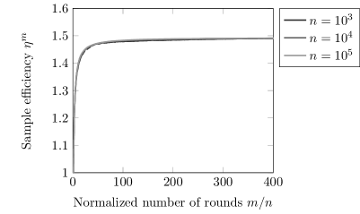
Figure 8.3: Sample efficiency for the Packing process versus the number of rounds over the number of bins $n$ for $n\in\{10^{3},10^{4},10^{5}\}$. The sample efficiency seems to converge to $1.5$.

The empirical results of Figure 8.3 strongly support this, suggesting that the sample efficiency of Packing is around $3/2$ on average.

Proof of 3.2.

We start with the following general expression for the expected number of balls allocated in an arbitrary round $t$,

$$\mathbf{E}\left[\,W^{t+1}-W^{t}\;\big{|}\;\mathfrak{F}^{t}\,\right]=\sum_{i:y_{i}^{t}\geqslant 0}1\cdot p_{i}+\sum_{i:y_{i}^{t}<0}\left(1+\left\lceil-y_{i}^{t}\right\rceil\right)\cdot p_{i}=1+\sum_{i:y_{i}^{t}<0}\left\lceil-y_{i}^{t}\right\rceil\cdot p_{i}.$$ (7.1)

Let $i^{*}$ be the smallest index such that $y_{i^{*}}^{t}<0$ and observe that the sequence $\left\lceil-y_{n}^{t}\right\rceil,\dots,\left\lceil-y_{i^{*}}^{t}\right\rceil$ is non-negative and non-increasing. Additionally, $\sum_{i=1}^{k}1/n\geqslant\sum_{i=1}^{k}p_{i}$ for all $k\in[n]$ by condition $\mathcal{P}$, and thus $\sum_{i=k}^{n}1/n\leqslant\sum_{i=k}^{n}p_{i}$ for any $i^{*}\leqslant k\leqslant n$. Hence, by Lemma A.1, we have

$$\sum_{i:y_{i}^{t}<0}\left\lceil-y_{i}^{t}\right\rceil\cdot p_{i}=\sum_{i=i^{*}}^{n}\left\lceil-y_{i}^{t}\right\rceil\cdot p_{i}\geqslant\sum_{i=i^{*}}^{n}\left\lceil-y_{i}^{t}\right\rceil\cdot\frac{1}{n}=\sum_{i:y_{i}^{t}<0}\left\lceil-y_{i}^{t}\right\rceil\cdot\frac{1}{n}.$$

Therefore, it follows from (7.1) that

$$\mathbf{E}\left[\,W^{t+1}-W^{t}\;\big{|}\;\mathfrak{F}^{t}\,\right]=1+\sum_{i:y_{i}^{t}<0}\left\lceil-y_{i}^{t}\right\rceil\cdot p_{i}\geqslant 1+\sum_{i:y_{i}^{t}<0}\left\lceil-y_{i}^{t}\right\rceil\cdot\frac{1}{n}.$$ (7.2)

Since $\Delta^{t}=\sum_{i=1}^{n}|y_{i}^{t}|$ and $\sum_{i=1}^{n}y_{i}^{t}=0$, we have $\mathbf{E}[\,W^{t+1}-W^{t}\mid\mathfrak{F}^{t}\,]\geqslant 1+\frac{\Delta^{t}}{2n}$ by (7.2). Thus,

$$\mathbf{E}\left[\,W^{t+1}-W^{t}\;\big{|}\;\mathfrak{F}^{t}\,\right]\cdot\mathbf{1}_{\{\Delta^{t}\geqslant n/10\}}\geqslant\left(1+\frac{1}{20}\right)\cdot\mathbf{1}_{\{\Delta^{t}\geqslant n/10\}}.$$ (7.3)

Recall that $B_{-}^{t}$ is the number of underloaded bins at time $t$. Thus by (7.2) we have

$$\mathbf{E}\left[\,W^{t+1}-W^{t}\;\big{|}\;\mathfrak{F}^{t}\,\right]\cdot\mathbf{1}_{\{|B_{-}^{t}|\geqslant n/20\}} \geqslant\left(1+\frac{n}{20}\cdot\frac{1}{n}\right)\cdot\mathbf{1}_{\{|B_{-}^{t}|\geqslant n/20\}}$$ (7.4)

$$=\left(1+\frac{1}{20}\right)\cdot\mathbf{1}_{\{|B_{-}^{t}|\geqslant n/20\}}.$$

For any $t_{0}\geqslant 1$, $t\in[t_{0},t_{0}+n]$, define $A$ to be the (random) set of times $t\in[t_{0},t_{0}+n]$ where the event $\mathcal{E}_{t}=\{\Delta^{t}\geqslant n/10\}\cup\{|B_{-}^{t}|\geqslant n/20\}$ holds. By (7.3) and (7.4) we have $\mathbf{E}\left[\,W^{t+1}-W^{t}\;\big{|}\;\mathfrak{F}^{t}\,\right]\mathbf{1}_{\mathcal{E}_{t}}\geqslant 1+1/20$. Then, since $W^{t+1}-W^{t}\geqslant 1$ for any $t$, for any $t_{0}\geqslant 1$,

$$\mathbf{E}\left[\,W^{t_{0}+n}-W^{t_{0}}\,\right] =\mathbf{E}\left[\,\sum_{t=t_{0}}^{t_{0}+n}\mathbf{E}\left[\,W^{t+1}-W^{t}\;\big{|}\;\mathfrak{F}^{t}\,\right]\mathbf{1}_{t\in\mathcal{E}_{t}}+\mathbf{E}\left[\,W^{t+1}-W^{t}\;\big{|}\;\mathfrak{F}^{t}\,\right]\mathbf{1}_{t\notin\mathcal{E}_{t}}\,\right]$$

$$\geqslant\mathbf{E}\left[\,|A|\cdot\left(1+\frac{1}{20}\right)+(n-|A|)\,\right].$$

Now, by Lemma 4.3 for any $t_{0}\geqslant 1$ we have $\mathbf{Pr}\left[\,|A|\geqslant n/40\,\right]=1$ and so

$$\mathbf{E}\left[\,W^{t_{0}+n}-W^{t_{0}}\,\right]\geqslant\mathbf{E}\left[\,\frac{n}{40}\cdot\left(1+\frac{1}{20}\right)+\frac{39n}{40}\,\right]=n\left(1+\frac{1}{800}\right).$$ (7.5)

Since the bound from (7.5) holds for any $t_{0}\geqslant 1$ the result follows for any $t>n$ (more details given below) however we must first consider the case $2\leqslant t\leqslant n$ separately.

Observe that in the first round we place one ball. Then, until $n$ balls have been placed we place two balls if we sample an underloaded bin and this is the most we can place in any round. We have little control how these are placed but certainly for any round $r\leqslant\lfloor n/3\rfloor$ there are at least $n-1-2\cdot(\lfloor n/3\rfloor-1)\geqslant\lceil n/3\rceil$ underloaded (empty) bins when we sample a bin. It follows from condition $\mathcal{P}$ that for any $r\leqslant\lfloor n/3\rfloor$ the number of underloaded bins sampled in the first $r$ rounds (excluding the first) stochastically dominates a $\operatorname{Bin}(r-1,1/3)$ random variable, which has median at least $\lfloor(r-1)/3\rfloor$. Thus, with probability at least $1/2$, at least $\lfloor(r-1)/3\rfloor$ of the first $r$ rounds contribute two balls. This is not greater than $0$ for $r\leqslant 6$, however for $2\leqslant r\leqslant 6$ at most $1+2\cdot 6=13$ bins are occupied. Thus for any $2\leqslant r\leqslant 6$ two balls are assigned in $r-1\geqslant 1$ of the first $r$ rounds (all rounds but the first) with probability at least $1-5\cdot(13/n)\geqslant 1/2$ by the union bound, since we assume throughout that $n$ is sufficiently large. Thus for any $2\leqslant r\leqslant\lfloor n/3\rfloor$ we have

$$\mathbf{E}\left[\,W^{r}\,\right]\geqslant r+\frac{1}{2}\cdot\max\left\{\lfloor(r-1)/3\rfloor,1\right\}\geqslant r\cdot\left(1+\frac{1}{12}\right).$$

If we assume (pessimistically) that only one ball is allocated at any round $t>\lfloor n/3\rfloor$, then for any $t\leqslant n$ we have

$$\mathbf{E}\left[\,W^{t}\,\right]\geqslant\mathbf{E}\left[\,W^{\min\{t,\lfloor n/3\rfloor\}}\,\right]+\min\{0,t-\lfloor n/3\rfloor\}\geqslant t\cdot\left(1+\frac{1}{50}\right).$$

Hence for any $2\leqslant t\leqslant n$ we have $\mathbf{E}[\,\mu^{t}\,]\geqslant\mathbf{E}\left[\,W^{t}\,\right]/t>1+1/50$. Also for any $t>n$ we have

$$\mathbf{E}[\,\mu^{t}\,] \geqslant\frac{1}{t}\cdot\left(\sum_{i=1}^{\lfloor(t-1)/n\rfloor}\mathbf{E}\left[\,W^{i\cdot n+1}-W^{(i-1)\cdot n+1}\,\right]+\left(t-\left\lfloor\frac{t-1}{n}\right\rfloor\cdot n\right)\right)$$

$$\geqslant\frac{1}{t}\cdot\left(t+\frac{1}{800}\left\lfloor\frac{t-1}{n}\right\rfloor\cdot n\right)\geqslant 1+\frac{1}{1600},$$

by (7.5). Thus taking $c=1+\frac{1}{1600}$ gives the lower bound on $\mathbf{E}[\,\mu^{t}\,]$.

For the upper bound, by Lemma 6.4, there exists a constant $\widetilde{c}>0$ such that for any $m\geqslant t_{0}\geqslant 0$,

$$\mathbf{E}\left[\,W^{m}-W^{t_{0}}\;\Big{|}\;\mathfrak{F}^{t_{0}}\,\right]\leqslant(\widetilde{c}+2)\cdot(m-t_{0}).$$

We now choose $m=t$ and $t_{0}=0$, and using $\mathbf{E}[\,W^{0}\,]=0$, we conclude

$$\mathbf{E}\left[\,W^{t}\,\right]\leqslant(\widetilde{c}+2)\cdot t.$$

Using this, and since for any process satisfying $\mathcal{P}$ and $\mathcal{W}$, we conclude that

$$\mathbf{E}[\,\mu^{t}\,]=\mathbf{E}\left[\frac{W^{t}}{t}\right]=\frac{\mathbf{E}\left[\,W^{t}\,\right]}{t}\leqslant\frac{(\widetilde{c}+2)\cdot t}{t}:=C,$$

for the constant $C=\widetilde{c}+2$. ∎

8 Experimental Results

In this section, we present some empirical results for the Packing, Tight-Packing and Memory processes (Figure 8.2 and Table 8.1) and compare their load with that of a $(1+\beta)$-process with $\beta=0.5$, a $\textsc{Quantile}(1/2)$ process, and the Two-Choice process.

$n$	$(1+\beta)$ for $\beta=1/2$	Packing	Tight-Packing	$\textsc{Quantile}(1/2)$	Memory	Two-Choice
$10^{3}$	12 :  5% 13 : 15% 14 : 31% 15 : 21% 16 : 15% 17 :  5% 18 :  4% 19 :  2% 20 :  1% 21 :  1%	6 :  3%  7 : 14%  8 : 30%  9 : 23% 10 : 15% 11 :  8% 12 :  4% 13 :  1% 14 :  1% 15 :  1%	5 : 23% 6 : 50% 7 : 15% 8 : 10% 9 :  1% 10 :  1%	3 :  1%  4 : 11%  5 : 46%  6 : 33%  7 :  6%  8 :  2% 10 :  1%	2 : 67% 3 : 33%	2 : 93% 3 :  7%
$10^{4}$	16 :  3% 17 : 21% 18 : 19% 19 : 10% 20 : 23% 21 : 11% 22 : 10% 23 :  2% 24 :  1%	9 :  2% 10 : 17% 11 : 28% 12 : 14% 13 : 22% 14 : 11% 15 :  3% 16 :  2% 17 :  1%	6 :  3% 7 : 24% 8 : 45% 9 : 23% 10 :  5%	6 : 14%  7 : 42%  8 : 25%  9 : 15% 10 :  2% 11 :  1% 12 :  1%	2 :  5% 3 : 95%	2 : 46% 3 : 54%
$10^{5}$	20 :  2% 21 :  7% 22 :  9% 23 : 26% 24 : 27% 25 : 14% 26 :  6% 27 :  3% 28 :  4% 29 :  1% 34 :  1%	12 :  2% 13 : 16% 14 : 20% 15 : 28% 16 : 23% 17 :  5% 18 :  3% 19 :  1% 20 :  2%	8 :  4% 9 : 33% 10 : 40% 11 : 17% 12 :  5% 13 :  1%	8 : 28%  9 : 42% 10 : 18% 11 :  7% 12 :  3% 14 :  1% 15 :  1%	3 : 100%	3 : 100%

Table 8.1: Summary of observed gaps for $n\in\{10^{3},10^{4},10^{5}\}$ bins and $m=1000\cdot n$ number of balls, for $100$ repetitions. The observed gaps are in bold and next to that is the $\%$ of runs where this was observed.

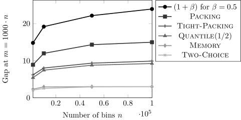
Figure 8.2: Average Gap vs. $n\in\{10^{3},10^{4},5\cdot 10^{4},10^{5}\}$ for the experimental setup of Table 8.1.

9 Conclusions

In this work, we introduced a new class of allocation processes we call Filling processes. Roughly speaking, these processes have a probability vector majorized by One-Choice, they allocate one ball when they sample an overloaded bin, but when they sample an underloaded bin they can allocate the number of missing balls to some arbitrary underloaded bins. We proved that any Filling process achieves an $\mathcal{O}(\log n)$ gap at an arbitrary round w.h.p. (3.1) and, for some constant $c>0$, allocates at least $1+c$ balls in each round in expectation (3.2).

Our prototype Filling process is Packing, which selects at each round a random bin, and if the bin is overloaded, allocates a single ball; otherwise it “fills” the underloaded bin with balls up until it becomes overloaded. For the Packing process we proved that the general upper bound of $\mathcal{O}(\log n)$ is tight for any sufficiently large $m$ (3.6). A consequence of 3.2 is that, in contrast to other processes with a gap that does not depend on the number of balls such as Two-Choice, $(1+\beta)$-process and $\textsc{Quantile}(1/2)$, Packing is more sample-efficient than One-Choice. Additionally we showed that, unlike Two-Choice, Packing can also handle arbitrarily biased distributions.

We also prove that our results for Filling processes can be extended to the Memory process by Mitzenmacher, Prabhakar and Shah [29]. Using this extension we prove the first $\mathcal{O}(\log n)$ gap bound for the Memory process with a polynomial number of balls.

There are several possible extensions to this work. One is to explore stronger versions of the conditions on the probability vector which imply $o(\log n)$ gap bounds. For example, it might be interesting to explore a version of Packing where the bin is sampled using Two-Choice.

At the opposite end, one might investigate probability vectors with weaker guarantees. In Section 3.4, we showed that for the Packing process with an arbitrarily $(a,b)$-biased sampling vector (which may even majorize One-Choice) the gap is w.h.p. at most $a\cdot\operatorname{poly}(n)$, i.e., still independent of $m$. This demonstrates the “power of filling” in balanced allocations.

Appendix A Auxiliary Inequalities

We provide an elementary proof of the following lemma for completeness; our proof is similar to that of [14, Lemma A.1]. This inequality also appears in [27, Ch. XII] where the authors state that it is a consequence of Abel’s transformation (summation by parts).

Lemma A.1.

Let the real sequences $(a_{k})_{k=1}^{n}$ and $(b_{k})_{k=1}^{n}$ be non-negative, and $(c_{k})_{k=1}^{n}$ be non-negative and non-increasing. If $\sum_{k=1}^{i}a_{k}\leqslant\sum_{k=1}^{i}b_{k}$ holds for all $1\leqslant i\leqslant n$ then,

$$\sum_{k=1}^{n}a_{k}\cdot c_{k}\leqslant\sum_{k=1}^{n}b_{k}\cdot c_{k}.$$ (A.1)

Proof.

We shall prove (A.1) holds by induction on $n\geqslant 1$. The base case $n=1$ follows immediately from the fact that $a_{1}\leqslant b_{1}$ and $c_{1}\geqslant 0$. Thus we assume $\sum_{k=1}^{n-1}a_{k}\cdot c_{k}\leqslant\sum_{k=1}^{n-1}b_{k}\cdot c_{k}$ holds for all sequences $(a_{k})_{k=1}^{n-1},(b_{k})_{k=1}^{n-1}$ and $(c_{k})_{k=1}^{n-1}$ satisfying the conditions of the lemma.

For the inductive step, suppose we are given sequences $(a_{k})_{k=1}^{n}$, $(b_{k})_{k=1}^{n}$ and $(c_{k})_{k=1}^{n}$ satisfying the conditions of the lemma. If $c_{2}=0$ then, since $(c_{k})_{k=1}^{n}$ is non-increasing and non-negative, $c_{k}=0$ for all $k\geqslant 2$. Thus as $a_{1}\leqslant b_{1}$ and $c_{1}\geqslant 0$ by the precondition of the lemma, we conclude

$$\sum_{k=1}^{n}a_{k}\cdot c_{k}=a_{1}\cdot c_{1}\leqslant b_{1}\cdot c_{1}=\sum_{k=1}^{n}b_{k}\cdot c_{k}.$$

We now treat the case $c_{2}>0$. Define the non-negative sequences $(a_{k}^{\prime})_{k=1}^{n-1}$ and $(b_{k}^{\prime})_{k=1}^{n-1}$ as follows:

• $a^{\prime}_{1}=\frac{c_{1}}{c_{2}}\cdot a_{1}+a_{2}$ and $a^{\prime}_{k}=a_{k+1}$ for $2\leqslant k\leqslant n-1$ ,

• $b^{\prime}_{1}=\frac{c_{1}}{c_{2}}\cdot b_{1}+b_{2}$ and $b^{\prime}_{k}=b_{k+1}$ for $2\leqslant k\leqslant n-1$,

Then as the inequalities $c_{1}\geqslant c_{2}$, $a_{1}\leqslant b_{1}$ and $\sum_{i=1}^{n}a_{k}\leqslant\sum_{i=1}^{n}b_{k}$ hold by assumption, we have

$$\sum_{k=1}^{n-1}a_{k}^{\prime}=\left(\frac{c_{1}}{c_{2}}-1\right)a_{1}+\sum_{k=1}^{n}a_{k}\leqslant\left(\frac{c_{1}}{c_{2}}-1\right)b_{1}+\sum_{k=1}^{n}b_{k}=\sum_{k=1}^{n-1}b_{k}^{\prime}.$$

Thus if we also let $(c_{k}^{\prime})_{k=1}^{n-1}=(c_{k+1})_{k=1}^{n-1}$, which is positive and non-increasing, then

$$\sum_{k=1}^{n-1}a_{k}^{\prime}\cdot c_{k}^{\prime}\leqslant\sum_{k=1}^{n-1}b_{k}^{\prime}\cdot c_{k}^{\prime},$$

by the inductive hypothesis. However

$$\sum_{k=1}^{n-1}a_{k}^{\prime}\cdot c_{k}^{\prime}=\left(\frac{c_{1}}{c_{2}}\cdot a_{1}+a_{2}\right)c_{2}+\sum_{k=2}^{n-1}a_{k+1}\cdot c_{k+1}=\sum_{k=1}^{n}a_{k}\cdot c_{k},$$

and likewise $\sum_{k=1}^{n-1}b_{k}^{\prime}\cdot c_{k}^{\prime}=\sum_{k=1}^{n}b_{k}\cdot c_{k}$. The result follows. ∎

Again, for completeness, we define Schur-convexity (see [26]) and state two basic results:

Definition A.2.

A function $f:\mathbb{R}^{n}\to\mathbb{R}$ is Schur-convex if for any non-decreasing $x,y\in\mathbb{R}^{n}$, if $x$ majorizes $y$ then $f(x)\geqslant f(y)$. A function $f$ is Schur-concave if $-f$ is Schur-convex.

Lemma A.3.

Let $g:\mathbb{R}\to\mathbb{R}$ be a convex (resp. concave) function. Then, the function $g(x_{1},\ldots,x_{n}):=\sum_{i=1}^{n}g(x_{i})$ is Schur-convex (resp. Schur-concave).

Lemma A.4.

For any $\alpha>0$, for any $\beta\in\mathbb{R}$ and any $\Delta\in\mathbb{R}$, consider the function

$$f(x_{1},x_{2},\ldots,x_{k})=\sum_{j=1}^{k}\exp\left(-\alpha x_{j}\right),$$

where $\sum_{j=1}^{k}x_{j}\geqslant\Delta$ and $x_{j}\geqslant\beta$ for all $1\leqslant j\leqslant k$. Then,

$$f(x_{1},x_{2},\ldots,x_{k})\leqslant(k-1)\cdot\exp\left(-\alpha\cdot\beta\right)+1\cdot\exp\left(-\alpha\cdot\left(\Delta-(k-1)\cdot\beta\right)\right).$$

Proof.

Note that by Lemma A.3, it follows that $f(x_{1},\ldots,x_{n})=\sum_{i=1}^{n}g(x_{i})$ is Schur-concave, since $g(z)=e^{-\alpha z}$ is concave for $\alpha>0$. As a consequence, the function attains its maximum if the values $(x_{1},x_{2},\ldots,x_{k})$ are as “spread out” as possible, i.e., if any prefix sum of the values ordered non-increasingly is as large as possible. ∎

Lemma A.5.

Consider any sequence $(z_{i})_{i\in\mathbb{N}}$ such that, for some $a>0$ and $b>0$, for every $i\geqslant 1$,

$$z_{i}\leqslant z_{i-1}\cdot a+b.$$

Then for every $i\in\mathbb{N}$,

$$z_{i}\leqslant z_{0}\cdot a^{i}+b\cdot\sum_{j=0}^{i-1}a^{j}.$$

Further, if $a<1$, then

$$z_{i}\leqslant z_{0}\cdot a^{i}+\frac{b}{1-a}.$$

Proof.

We will prove the first claim by induction. For $i=0$, $z_{0}\leqslant z_{0}$. Assume the induction hypothesis holds for some $i\geqslant 0$, then since $a>0$,

$$z_{i+1}\leqslant z_{i}\cdot a+b\leqslant\Big{(}z_{0}\cdot a^{i}+b\cdot\sum_{j=0}^{i-1}a^{j}\Big{)}\cdot a+b=z_{0}\cdot a^{i+1}+b\cdot\sum_{j=0}^{i}a^{j}.$$

Hence, the first claim follows. The second part of the claim is immediate, since for $a\in(0,1)$, $\sum_{j=0}^{\infty}a^{j}=\frac{1}{1-a}$. ∎

Appendix B Counterexample for the Exponential Potential Function

In this section, we present a configuration for which the exponential potential function $\Phi$ (such as the one defined in Section 4), increases by a multiplicative factor in expectation, in a round $t$ where the “good event” $\mathcal{G}^{t}$ does not hold.

Claim B.1.

For any constant $\alpha>0$ and for sufficiently large $n$, consider the (normalized) load configuration,

$$y^{t}=(\sqrt{n},\underbrace{0,\ldots,0}_{n-\sqrt{n}-1\text{ bins}},\underbrace{-1,\ldots,-1}_{\sqrt{n}\text{ bins}}).$$

Then, for the Packing process, the potential function $\Phi^{t}:=\sum_{i:y_{i}^{t}\geqslant 0}e^{\alpha y_{i}^{t}}$ will increase in expectation, i.e.,

$$\mathbf{E}[\,\Phi^{t+1}\mid\mathfrak{F}^{t}\,]\geqslant\Phi^{t}\cdot\Big{(}1+0.1\cdot\frac{\alpha^{2}}{n}\Big{)}.$$

Proof.

Consider the contribution of bin $i=1$, with $y_{1}^{t}=\sqrt{n}$.

$$\mathbf{E}[\,\Phi_{1}^{t+1}\mid\mathfrak{F}^{t}\,]$$

$$\quad=e^{\alpha\sqrt{n}}\cdot\Big{(}1+\frac{1}{n}\cdot(e^{\alpha-\alpha/n}-1)+\frac{n-\sqrt{n}-1}{n}\cdot(e^{-\alpha/n}-1)+\frac{\sqrt{n}}{n}\cdot(e^{-2\alpha/n}-1)\Big{)}.$$

Now using a Taylor estimate $e^{z}\geqslant 1+z+0.3z^{2}$ for $z\geqslant-1.5$,

$$\mathbf{E}[\,\Phi_{1}^{t+1}\mid\mathfrak{F}^{t}\,] \geqslant e^{\alpha\sqrt{n}}\cdot\Big{(}1+\frac{1}{n}\cdot\Big{(}\alpha-\frac{\alpha}{n}+0.3\cdot\Big{(}\alpha-\frac{\alpha}{n}\Big{)}^{2}\Big{)}$$

$$\qquad+\frac{n-\sqrt{n}-1}{n}\cdot\Big{(}-\frac{\alpha}{n}+0.3\cdot\frac{\alpha^{2}}{n^{2}}\Big{)}+\frac{\sqrt{n}}{n}\cdot\Big{(}-\frac{2\alpha}{n}+1.2\cdot\frac{\alpha^{2}}{n^{2}}\Big{)}\Big{)}$$

$$=e^{\alpha\sqrt{n}}\cdot\Big{(}1+\frac{\alpha+0.3\cdot\alpha^{2}}{n}-\frac{\alpha}{n}+o(n^{-1})\Big{)}$$

$$=e^{\alpha\sqrt{n}}\cdot\Big{(}1+0.3\cdot\frac{\alpha^{2}}{n}+o(n^{-1})\Big{)}$$

$$\geqslant e^{\alpha\sqrt{n}}\cdot\Big{(}1+0.2\cdot\frac{\alpha^{2}}{n}\Big{)}.$$

At round $t$, the contribution of the rest of the bins is at most $n$, i.e., $\sum_{i>1,y_{i}^{t}\geqslant 0}\Phi^{t}\leqslant n$. Note that since $\alpha$ is a constant for sufficiently large $n$, we have $n\cdot(1+0.1\cdot\frac{\alpha^{2}}{n})<0.1\cdot\alpha^{2}\cdot e^{\alpha\sqrt{n}}$. Hence,

$$\mathbf{E}[\,\Phi^{t+1}\mid\mathfrak{F}^{t}\,] \geqslant e^{\alpha\sqrt{n}}\cdot\Big{(}1+0.2\cdot\frac{\alpha^{2}}{n}\Big{)}=e^{\alpha\sqrt{n}}\cdot\Big{(}1+0.1\cdot\frac{\alpha^{2}}{n}\Big{)}+0.1\cdot\frac{\alpha^{2}}{n}\cdot e^{\alpha\sqrt{n}}$$

$$\geqslant\Phi_{1}^{t}\cdot\Big{(}1+0.1\cdot\frac{\alpha^{2}}{n}\Big{)}+n\cdot(1+0.1\cdot\frac{\alpha^{2}}{n})$$

$$\geqslant\Phi_{1}^{t}\cdot\Big{(}1+0.1\cdot\frac{\alpha^{2}}{n}\Big{)}+\left(\sum_{i>1,y_{i}^{t}\geqslant 0}\Phi^{t}\right)\cdot\Big{(}1+0.1\cdot\frac{\alpha^{2}}{n}\Big{)}$$

$$=\Phi^{t}\cdot\Big{(}1+0.1\cdot\frac{\alpha^{2}}{n}\Big{)},$$

as claimed. ∎

References

- [1]
- Augustine et al. [2016] John Augustine, William K. Moses Jr., Amanda Redlich, and Eli Upfal. Balanced Allocation: Patience is not a Virtue. In 27th Annual ACM-SIAM Symposium on Discrete Algorithms (SODA’16). SIAM, 655–671. doi
- Azar et al. [1999] Yossi Azar, Andrei Z. Broder, Anna R. Karlin, and Eli Upfal. Balanced allocations. SIAM J. Comput. 29, 1 (1999), 180–200. doi
- Bansal and Feldheim [2022] Nikhil Bansal and Ohad N. Feldheim. The power of two choices in graphical allocation. In 54th Annual ACM Symposium on Theory of Computing (STOC’22). ACM, 52–63. doi
- Bansal and Kuszmaul [2022] Nikhil Bansal and William Kuszmaul. Balanced Allocations: The Heavily Loaded Case with Deletions. In 63rd Annual IEEE Symposium on Foundations of Computer Science (FOCS’22). IEEE, 801–812. doi
- Berenbrink et al. [2006] Petra Berenbrink, Artur Czumaj, Angelika Steger, and Berthold Vöcking. Balanced allocations: the heavily loaded case. SIAM J. Comput. 35, 6 (2006), 1350–1385. doi
- Celis et al. [2011] L. Elisa Celis, Omer Reingold, Gil Segev, and Udi Wieder. Balls and Bins: Smaller Hash Families and Faster Evaluation. In 52nd Annual IEEE Symposium on Foundations of Computer Science (FOCS’11). IEEE, 599–608.
- Cole et al. [1998] Richard Cole, Alan Frieze, Bruce M. Maggs, Michael Mitzenmacher, Andréa W. Richa, Ramesh Sitaraman, and Eli Upfal. On balls and bins with deletions. In 2nd International Workshop on Randomization and Computation (RANDOM’98), Vol. 1518. Springer, Berlin, 145–158. doi
- Czumaj and Stemann [2001] Artur Czumaj and Volker Stemann. Randomized allocation processes. Random Structures & Algorithms 18, 4 (2001), 297–331. doi
- Dwivedi et al. [2019] Raaz Dwivedi, Ohad N. Feldheim, Ori Gurel-Gurevich, and Aaditya Ramdas. The power of online thinning in reducing discrepancy. Probab. Theory Related Fields 174, 1-2 (2019), 103–131. doi
- Eager et al. [1986] Derek L. Eager, Edward D. Lazowska, and John Zahorjan. Adaptive load sharing in homogeneous distributed systems. IEEE Transactions on Software Engineering SE-12, 5 (1986), 662–675. doi
- Feldheim and Gurel-Gurevich [2021] Ohad N. Feldheim and Ori Gurel-Gurevich. The power of thinning in balanced allocation. Electron. Commun. Probab. 26 (2021), Paper No. 34, 8. doi
- Feldheim et al. [pear] Ohad N. Feldheim, Ori Gurel-Gurevich, and Jiange Li. Long-term balanced allocation via thinning. The Annals of Applied Probability (to appear), arXiv:2110.05009.
- Friedrich et al. [2012] Tobias Friedrich, Martin Gairing, and Thomas Sauerwald. Quasirandom Load Balancing. SIAM J. Comput. 41, 4 (2012), 747–771. doi
- Godfrey [2008] P. Brighten Godfrey. Balls and bins with structure: balanced allocations on hypergraphs. In 19th Annual ACM-SIAM Symposium on Discrete Algorithms (SODA’08). ACM, 511–517.
- Greenhill et al. [2023] Catherine Greenhill, Bernard Mans, and Ali Pourmiri. Balanced allocation on hypergraphs. J. Comput. System Sci. 138 (2023), 103459. doi
- Iwama and Kawachi [2005] Kazuo Iwama and Akinori Kawachi. Approximated Two Choices in Randomized Load Balancing. In Algorithms and Computation. Springer Berlin Heidelberg, 545–557.
- Karp et al. [1996] Richard M. Karp, Michael Luby, and Friedhelm Meyer auf der Heide. Efficient PRAM simulation on a distributed memory machine. Algorithmica 16, 4-5 (1996), 517–542. doi
- Kenthapadi and Panigrahy [2006] Krishnaram Kenthapadi and Rina Panigrahy. Balanced allocation on graphs. In 17th Annual ACM-SIAM Symposium on Discrete Algorithms (SODA’06). ACM, 434–443. doi
- Los and Sauerwald [2022] Dimitrios Los and Thomas Sauerwald. Balanced Allocations with Incomplete Information: The Power of Two Queries. In 13th Innovations in Theoretical Computer Science Conference (ITCS’22), Vol. 215. Schloss Dagstuhl - Leibniz-Zentrum für Informatik, 103:1–103:23. doi
- Los et al. [2022] Dimitrios Los, Thomas Sauerwald, and John Sylvester. Balanced Allocations: Caching and Packing, Twinning and Thinning. In 33rd Annual ACM-SIAM Symposium on Discrete Algorithms (SODA’22). SIAM, 1847–1874. doi
- Los et al. [2023a] Dimitrios Los, Thomas Sauerwald, and John Sylvester. Balanced Allocations with Heterogeneous Bins: The Power of Memory. In 34th Annual ACM-SIAM Symposium on Discrete Algorithms (SODA’23). SIAM, 4448–4477. doi
- Los et al. [2023b] Dimitrios Los, Thomas Sauerwald, and John Sylvester. 2023b. Mean-Biased Processes for Balanced Allocations. arXiv:2308.05087 [math.PR]
- Lu et al. [2011] Yi Lu, Qiaomin Xie, Gabriel Kliot, Alan Geller, James R. Larus, and Albert G. Greenberg. Join-Idle-Queue: A novel load balancing algorithm for dynamically scalable web services. Perform. Evaluation 68, 11 (2011), 1056–1071. doi
- Luczak and Norris [2013] M. J. Luczak and J. R. Norris. Averaging over fast variables in the fluid limit for Markov chains: application to the supermarket model with memory. Ann. Appl. Probab. 23, 3 (2013), 957–986. doi
- Marshall et al. [2011] Albert W. Marshall, Ingram Olkin, and Barry C. Arnold. 2011. Inequalities: theory of majorization and its applications (second ed.). Springer, New York. doi
- Mitrinović et al. [1993] D. S. Mitrinović, J. E. Pečarić, and A. M. Fink. 1993. Classical and new inequalities in analysis. Mathematics and its Applications (East European Series), Vol. 61. Kluwer Academic Publishers Group, Dordrecht. doi
- Mitzenmacher [1999] M. Mitzenmacher. On the analysis of randomized load balancing schemes. Theory Comput. Syst. 32, 3 (1999), 361–386. doi
- Mitzenmacher et al. [2002] Michael Mitzenmacher, Balaji Prabhakar, and Devavrat Shah. Load Balancing with Memory. In 43rd Annual IEEE Symposium on Foundations of Computer Science (FOCS’02). IEEE, 799–808. doi
- Mitzenmacher et al. [2001] Michael Mitzenmacher, Andréa W. Richa, and Ramesh Sitaraman. 2001. The power of two random choices: a survey of techniques and results. In Handbook of randomized computing, Vol. I, II. Comb. Optim., Vol. 9. Kluwer Acad. Publ., Dordrecht, 255–312. doi
- Mitzenmacher and Upfal [2017] Michael Mitzenmacher and Eli Upfal. 2017. Probability and computing (second ed.). Cambridge University Press, Cambridge. Randomization and probabilistic techniques in algorithms and data analysis.
- Peres et al. [2015] Yuval Peres, Kunal Talwar, and Udi Wieder. Graphical balanced allocations and the -choice process. Random Structures & Algorithms 47, 4 (2015), 760–775. doi
- Raab and Steger [1998] Martin Raab and Angelika Steger. 1998. “Balls into bins”—a simple and tight analysis. In Proceedings of 2nd International Workshop on Randomization and Approximation Techniques in Computer Science (RANDOM’98). Vol. 1518. Springer, 159–170. doi
- Spencer [1977] Joel Spencer. Balancing games. J. Combinatorial Theory Ser. B 23, 1 (1977), 68–74. doi
- Wieder [2007] Udi Wieder. Balanced allocations with heterogenous bins. In 19th Annual ACM Symposium on Parallel Algorithms and Architectures (SPAA’07). ACM, 188–193. doi
- Wieder [2017] Udi Wieder. Hashing, Load Balancing and Multiple Choice. Found. Trends Theor. Comput. Sci. 12, 3-4 (2017), 275–379. doi