Transformation-Invariant Learning of Optimal Individualized Decision Rules with Time-to-Event Outcomes

Abstract

In many important applications of precision medicine, the outcome of interest is time to an event (e.g., death, relapse of disease) and the primary goal is to identify the optimal individualized decision rule (IDR) to prolong survival time. Existing work in this area have been mostly focused on estimating the optimal IDR to maximize the restricted mean survival time in the population. We propose a new robust framework for estimating an optimal static or dynamic IDR with time-to-event outcomes based on an easy-to-interpret quantile criterion. The new method does not need to specify an outcome regression model and is robust for heavy-tailed distribution. The estimation problem corresponds to a nonregular M-estimation problem with both finite and infinite-dimensional nuisance parameters. Employing advanced empirical process techniques, we establish the statistical theory of the estimated parameter indexing the optimal IDR. Furthermore, we prove a novel result that the proposed approach can consistently estimate the optimal value function under mild conditions even when the optimal IDR is non-unique, which happens in the challenging setting of exceptional laws. We also propose a smoothed resampling procedure for inference. The proposed methods are implemented in the R-package QTOCen. We demonstrate the performance of the proposed new methods via extensive Monte Carlo studies and a real data application.

KEY WORDS: Exceptional laws, individualized decision rule, inference, precision medicine, robust method, time-to-event data.

1 Introduction

The problem of estimating the optimal individualized decision rule (IDR) has recently received substantial attention in precision medicine and other domains. A treatment can be a drug, a therapy, or any other actionable choice (or a sequence of such choices) such as a policy or program. The goal of optimal IDR estimation is to determine a decision rule that assigns a subject to one of the treatment options based on individual information available each decision point such that some functional of the potential outcome distribution is optimized.

For completely observed data, several successful approaches exist for estimating the optimal IDR, including Q-learning (Watkins and Dayan,, 1992; Murphy, 2005b, ; Chakraborty et al.,, 2010; Song et al.,, 2015), A-learning (Robins et al.,, 2000; Murphy,, 2003; Murphy, 2005a, ; Moodie and Richardson,, 2010), model-free or policy search methods (Robins and Rotnitzky,, 2008; Orellana and Robins,, 2010; Zhang et al.,, 2012; Zhao et al.,, 2012; Zhao et al., 2015b, ), the interpretation-enhanced tree or list-based methods (Laber and Zhao,, 2015; Cui et al.,, 2017; Zhu et al.,, 2017; Zhang et al.,, 2018) among others. See also the books of Chakraborty and Moodie, (2013) and Kosorok and Moodie, (2016) for a general introduction and additional references.

The focus of this paper is on estimating the optimal static (one-stage) or dynamic (multi-stage) IDR for time-to-event or survival data, where the outcome is possibly censored. Several new challenges arise when analyzing such data compared with the complete data case. Censoring occurs when an individual drops out from the study or the study ends before the subject experiences the event of interest. The distribution of survival time (e.g., time to death, onset of disease) is often highly skewed. The situation gets even more complicated for estimating the optimal dynamic IDR, where the data are collected longitudinally. Consider the setting where the treatment decisions for a patient are made at $k$ pre-specified decision points. Each decision is allowed to depend on the patient’s characteristics (e.g., gender, age) and treatment history (e.g., disease progression status and how the individual responds to previous treatments) up to that decision point. The patient may be censored at any stage of treatment. Direct application of existing complete-data techniques could result in severe bias, as demonstrated in the Monte Carlo studies in Section 5.

Several authors have recently investigated estimating the optimal IDR with survival data, see Goldberg and Kosorok, (2012), Xu et al., (2016), Jiang et al., 2017a , Jiang et al., 2017b , Bai et al., (2017), Hager et al., (2018), Xu et al., (2016), Díaz et al., (2018), Simoneau et al., (2020), among others. For time-to-event outcomes, new criterion is needed to evaluate the effectiveness of an IDR. Of crucial importance is that such a criterion can be reliably estimated under censoring. The existing work have been mostly focused on maximizing the restricted mean survival time in the population.

We consider time-to-event outcomes and propose a new robust framework for estimating the optimal IDR using an alternative criterion based on the marginal quantile of the potential outcome distribution. The new optimality criterion is easy to interpret. Median survival time has already been popularly used clinically to evaluate the success of cancer treatment. It can be reliably estimated even under relatively heavy censoring (e.g., the censoring rate is more than 50% in the real data example of this paper). The resulted optimal IDR is invariant under monotone-transformation of the outcome. We develop robust estimation methods for both static and dynamic optimal IDRs. The robust approach circumvents the difficulty of specifying a reliable outcome regression model, especially for the dynamic setting which demands a sequence of generative regression models.

We consider estimating the optimal IDR in a class of candidate decision rules indexed by a finite-dimensional parameter. The estimation problem corresponds to a challenging non-regular M-estimation problem with both finite and infinite-dimensional nuisance parameters, due to the unknown censoring distribution. For the optimal static IDR, we rigorously establish the cube-root convergence rate for the estimated parameter by employing modern empirical processes techniques. We prove that its asymptotic distribution corresponds to the maximizer of a centered Gaussian process with a parabolic drift. It is worth emphasizing that the nonstandard asymptotics is due to the intrinsic nature of the decision problem, which relates to a sharp edge effect in the decision function. Due to the nature of nonstandard asymptotics, the problem is substantially harder than regular M-estimation problem with infinite-dimensional nuisance parameters.

Moreover, we establish a useful novel result that shows the optimal value can be consistently estimated under weak conditions for the challenging setting of exceptional laws. Under exceptional laws, there exists a subgroup of patients for whom the treatment is neither beneficial nor harmful. In this case, the optimal IDR is non-unique, see for example, the discussions in Robins and Rotnitzky, (2014) and Luedtke and van der Laan, (2016).

Theoretically, our work complements existing results and significantly enhances the knowledge about optimal IDR estimation with survival data. The existing results have been mostly focused on prediction error bounds and have not studied the properties of the estimated parameter indexing the optimal IDR. Furthermore, to the best of our knowledge, existing work on optimal IDR estimation with survival outcomes assume non-exceptional laws and thus avoid the problem of optimal value estimation under exceptional laws.

The rest of the paper is organized as follows. Section 2 introduces the new framework and the robust method for estimating an optimal static IDR with survival data, with theoretical properties developed in Section 3. Section 4 presents the estimation method and the theory for the dynamic IDR setting. In Section 5, we report results from extensive Monte Carlo studies. In Section 6, we illustrate the application on the analysis of a breast cancer data set. The proposed methods are implemented in the R-package QTOCen. The regularity conditions are given in the Appendix. The technical derivations and additional numerical results are given in the online supplement.

2 Robust estimation for static optimal IDR

2.1 Preliminaries

We first consider the single-stage setting. Let $A\in\{0,1\}$ denote the binary treatment, ${\bm{X}}\in\mathbb{R}^{p}$ denote the vector of covariates with support $\mathcal{X}$, and $T\in\mathbb{R}^{+}$ denote the time to the event of interest (or a transformation thereof). We often refer to $T$ as survival time. Without loss of generality, we assume that a larger value of $T$ indicates better treatment effect. The outcome $T$ may not be observed due to censoring. Let $C\in\mathbb{R}^{+}$ denote the censoring variable and $\Delta=I(T\leq C)$. If the observation is censored (i.e., $\Delta=0$), then we only observe $C$. Let $Y=\min\{T,C\}$ be the observed outcome. The observed data consist of $\big{\{}{\bm{X}}_{i},A_{i},Y_{i},\Delta_{i}\big{\}}$, $i=1,\ldots,n$, which are independent copies of $\big{(}{\bm{X}},A,Y,\Delta\big{)}$.

To assess the treatment effect, we adopt the potential outcome framework (Neyman,, 1923; Rubin,, 1978) in causal inference. The $i$-th subject has two potential outcomes: ${T^{\ast}_{i}\big{(}0\big{)}}$ and ${T^{\ast}_{i}\big{(}1\big{)}}$, where $T_{i}^{*}(0)$ is the survival time had the subject received treatment 0 and $T_{i}^{*}(1)$ is defined similarly, $i=1,...,n$. In practice, a subject receives one and only one of the two possible treatments. Under the stable unit treatment value assumption (Rubin, (1986)), we have $T_{i}=A_{i}{T^{\ast}_{i}\big{(}1\big{)}}+\big{(}1-A_{i}\big{)}{T^{\ast}_{i}\big{(}0\big{)}}.$ That is, the survival time of the $i$th subject is the potential survival time corresponding to the treatment that subject actually received. Furthermore, we assume the no unmeasured confounders assumption (Rosenbaum and Rubin,, 1983) is satisfied, i.e., $\{T_{i}^{*}(0),T_{i}^{*}(1)\}$ are independent of $A_{i}$ conditional on ${\bm{X}}_{i}$. This is a common assumption in causal inference and is automatically satisfied for a randomized trial. Mathematically, an IDR $d({\bm{X}})$ is a mapping from the space of covariates $\mathcal{X}$ to the space of candidate treatments $\{0,1\}$. The potential outcome associated with $d({\bm{X}})$ is denoted by ${T^{\ast}\big{(}d({\bm{X}})\big{)}}$. We have ${T^{\ast}\big{(}d({\bm{X}})\big{)}}={T^{\ast}\big{(}1\big{)}}d\big{(}{\bm{X}}\big{)}+{T^{\ast}\big{(}0\big{)}}\big{[}1-d\big{(}{\bm{X}}\big{)}\big{]}.$

2.2 New optimality criterion for evaluating IDR with time-to-event outcome

Different from the completely observed data case, the mean of the outcome is usually difficult to estimate accurately at the presence of censoring. The most popular criterion in the existing literature for time-to-event data is the restricted mean survival time $\mbox{E}\{\min\big{(}{T^{\ast}\big{(}d({\bm{X}})\big{)}},L\big{)}\}$, where $L$ is a user-supplied cut-off time. In this paper, we consider an alternative criterion for comparing IDRs for time-to-event outcomes based on the marginal quantile treatment effect. The new criterion enjoys three appealing properties: easy to interpret, robust to long-tailed survival distribution, and invariant to the monotone transformation of survival time. The marginal $\tau$-th quantile ($0<\tau<1$) of the potential outcome ${T^{\ast}\big{(}d({\bm{X}})\big{)}}$ is defined as

$$Q_{\tau}\big{\{}{T^{\ast}\big{(}d({\bm{X}})\big{)}}\big{\}}=\inf\Big{\{}t\in\mathbb{R}:P\big{\{}{T^{\ast}\big{(}d({\bm{X}})\big{)}}\leq t\big{\}}\geq\tau\Big{\}},$$

where $P$ denotes the marginal distribution of ${T^{\ast}\big{(}d({\bm{X}})\big{)}}$. In IDR estimation problems, $Q_{\tau}\big{\{}{T^{\ast}\big{(}d({\bm{X}})\big{)}}\big{\}}$ is referred to as the value function. We sometimes use the short-hand notation $Q_{\tau}\{T^{\ast}(d)\}$. Given a class $\mathcal{D}$ of candidate IDRs, the optimal IDR is defined as

$$d_{opt}({T^{\ast}\big{(}d({\bm{X}})\big{)}})=\underset{d\in\mathcal{D}}{\arg\max}\ Q_{\tau}\big{\{}{T^{\ast}\big{(}d({\bm{X}})\big{)}}\big{\}}.$$ (1)

As an example, the above optimal IDR with $\tau=0.5$ will lead to the maximal median of the potential survival time if each individual in the population follows the treatment recommended. In some other applications (e.g., distributing aid in a social welfare program), we may target improving the lower quantile by considering a smaller value of $\tau$. For an arbitrary monotone transformation $h(\cdot)$, it is known that $h\big{(}Q_{\tau}\{h({T^{\ast}\big{(}d\big{)}})\}\big{)}=Q_{\tau}\{h({T^{\ast}\big{(}d\big{)}})\}$ (Koenker,, 2005). Hence, the same decision will be reached no matter the analysis is based on the original survival time or its monotonic transformation.

For complete data, quantile criterion was studied in Wang et al., (2018) but their work is not applicable to survival data, which is also theoretically substantially harder with the presence of an infinite-dimensional nuisance parameter due to censoring. Wahed, (2009) studied estimating the survival quantiles in two-stage randomization designs with fixed IDRs but had not investigated the more challenging problem of optimal IDR estimation.

In practice, $\mathcal{D}$ is usually chosen to be a class of IDRs indexed by a Euclidean parameter for interpretability. Same as Zhang et al., (2012) and others, we focus on the class of index rules $\mathcal{D}=\Big{\{}{d_{{\bm{\beta}}}\big{(}{\bm{X}}\big{)}}=\mbox{I}\big{(}{\bm{\beta}}^{{T}}{\bm{X}}>0\big{)}:\ \ |\beta_{1}|=1,\ \widetilde{{\bm{\beta}}}\in\mathbb{B}\Big{\}},$ where ${\bm{\beta}}=(\beta_{1},...,\beta_{p})^{T}=(\beta_{1},\widetilde{\bm{\beta}}^{T})^{T}$, $\mathbb{B}$ is a compact subset of $\mathbb{R}^{p-1}$ and $\mbox{I}(\cdot)$ denotes the indicator function. For identifiability, we assume there exists a continuous covariate whose coefficient has absolute value one. Without loss of generality, we assume $|\beta_{1}|=1$. The population parameter ${\bm{\beta}}_{0}=(\beta_{01},...,\beta_{0p})^{T}$ indexing the optimal IDR is

$${\bm{\beta}}_{0}=\underset{{\bm{\beta}}\in\mathbb{B}^{o}}{\arg\max}Q_{\tau}\{{T^{\ast}\big{(}d({\bm{X}})\big{)}}\},$$

where $\mathbb{B}^{o}=\{{\bm{\beta}}\in\mathbb{R}^{p}:|\beta_{1}|=1,\ \tilde{{\bm{\beta}}}\in\mathbb{B}\}$.

2.3 A robust estimation procedure

Based on the observations $\big{\{}{\bm{X}}_{i},A_{i},Y_{i},\Delta_{i}\big{\}}$, $i=1,\ldots,n$, our goal is to estimate the population parameter ${\bm{\beta}}_{0}$ indexing the optimal IDR. It is known that a misspecified generative regression model can result in severe bias in estimating the optimal treatment (Qian and Murphy,, 2011; Zhang et al.,, 2012; Zhao et al.,, 2012; Zhao et al., 2015a, ). We introduce a robust estimator that accounts for censoring while at the same time circumvents the difficulty of specifying a reliable generative regression model.

Given an IDR $d_{{\bm{\beta}}}({\bm{X}})$, the treatment it would recommend to subject $i$ may or may not coincide with the treatment the subject actually received. Even if $A_{i}=d_{{\bm{\beta}}}({\bm{X}}_{i})$, we may not observe ${T^{\ast}_{i}\{d_{{\bm{\beta}}}\big{(}{\bm{X}}_{i}\big{)}\}}$ if the subject is censored. To obtain a consistent estimator for $Q_{\tau}\{{T^{\ast}_{i}\{d_{{\bm{\beta}}}\big{(}{\bm{X}}_{i}\big{)}\}}\}$, we adapt the induced missing data framework in Zhang et al., (2012) to time-to-event data. Specifically, we consider an artificial missing data structure with the missing data indicator ${R_{i}\big{(}{\bm{\beta}}\big{)}}=\big{[}A_{i}{d_{{\bm{\beta}}}\big{(}{\bm{X}}_{i}\big{)}}+\big{(}1-A_{i}\big{)}\big{\{}1-{d_{{\bm{\beta}}}\big{(}{\bm{X}}_{i}\big{)}}\big{\}}\big{]}\Delta_{i}.$ The observed outcome $Y_{i}$ is equal to the potential outcome ${T^{\ast}_{i}\{d_{{\bm{\beta}}}\big{(}{\bm{X}}_{i}\big{)}\}}$ only if ${R_{i}\big{(}{\bm{\beta}}\big{)}}=1$. In this framework, the “full data” that we may not completely observe consist of $\{{\bm{X}}_{i},{T^{\ast}_{i}\{d_{{\bm{\beta}}}\big{(}{\bm{X}}_{i}\big{)}\}}\}_{i=1}^{n}$, and the observed data consist of $\big{\{}{\bm{X}}_{i},{R_{i}\big{(}{\bm{\beta}}\big{)}},{R_{i}\big{(}{\bm{\beta}}\big{)}}{T^{\ast}_{i}\{d_{{\bm{\beta}}}\big{(}{\bm{X}}_{i}\big{)}\}}\big{\}}=\big{\{}{\bm{X}}_{i},{R_{i}\big{(}{\bm{\beta}}\big{)}},{R_{i}\big{(}{\bm{\beta}}\big{)}}Y_{i}\big{\}}_{i=1}^{n}$.

Let $\pi_{A}({\bm{X}}_{i})=P(A_{i}=1|{\bm{X}}_{i})$ be the propensity score; and let ${G_{C}}\big{(}t|{\bm{X}},A\big{)}=P\big{(}C>t|{\bm{X}},A\big{)}$ denote the conditional survival function of $C$ given $\{{\bm{X}},A\}$. Let $\pi_{i}\big{(}{\bm{\beta}}\big{)}={P}\bigl{\{}{R_{i}\big{(}{\bm{\beta}}\big{)}}=1\mid{\bm{X}}_{i},{T^{\ast}_{i}\big{(}1\big{)}},{T^{\ast}_{i}\big{(}0\big{)}}\bigr{\}}$ be the probability of missingness conditional on the full data. We observe

$$\pi_{i}\big{(}{\bm{\beta}}\big{)}$$

$$=\ \pi_{A}({\bm{X}}_{i}){d_{{\bm{\beta}}}\big{(}{\bm{X}}_{i}\big{)}}{P}\bigl{[}\Delta_{i}=1\mid{\bm{X}}_{i},{T^{\ast}_{i}\big{(}1\big{)}},{T^{\ast}_{i}\big{(}0\big{)}},A_{i}=1\bigr{]}$$

$$+(1-\pi_{A}({\bm{X}}_{i}))(1-{d_{{\bm{\beta}}}\big{(}{\bm{X}}_{i}\big{)}}){P}\bigl{[}\Delta_{i}=1\mid{\bm{X}}_{i},{T^{\ast}_{i}\big{(}1\big{)}},{T^{\ast}_{i}\big{(}0\big{)}},A_{i}=0\bigr{]}$$

$$=\ \big{\{}\pi_{A}({\bm{X}}_{i}){d_{{\bm{\beta}}}\big{(}{\bm{X}}_{i}\big{)}}+(1-\pi_{A}({\bm{X}}_{i}))(1-{d_{{\bm{\beta}}}\big{(}{\bm{X}}_{i}\big{)}})\big{\}}{G_{C}}\Big{(}{T^{\ast}_{i}\{d_{{\bm{\beta}}}\big{(}{\bm{X}}_{i}\big{)}\}}\big{|}{\bm{X}},A_{i}={d_{{\bm{\beta}}}\big{(}{\bm{X}}_{i}\big{)}}\Big{)}.$$

Note that for the complete cases (corresponding to ${R_{i}\big{(}{\bm{\beta}}\big{)}}=1$), we have $Y_{i}={T^{\ast}_{i}\{d_{{\bm{\beta}}}\big{(}{\bm{X}}_{i}\big{)}\}}$ and the corresponding

$$\pi_{i}\big{(}{\bm{\beta}}\big{)}=\ \big{[}\pi_{A}({\bm{X}}_{i}){d_{{\bm{\beta}}}\big{(}{\bm{X}}_{i}\big{)}}+\big{(}1-\pi_{A}({\bm{X}}_{i})\big{)}\big{(}1-{d_{{\bm{\beta}}}\big{(}{\bm{X}}_{i}\big{)}}\big{)}\big{]}{G_{C}}\big{(}Y_{i}\big{|}{\bm{X}},A_{i}\big{)}.$$

To estimate ${\bm{\beta}}_{0}$, we propose the following two-step estimator. First, we estimate ${Q_{\tau}\big{\{}T^{\ast}\big{(}d_{{\bm{\beta}}}({\bm{X}})\big{)}\big{\}}}$ by the following inverse probability weighted estimator

$${\widehat{Q}_{\tau}\big{\{}T^{\ast}\big{(}d_{{\bm{\beta}}}({\bm{X}})\big{)}\big{\}}}=\arg\min\limits_{\begin{subarray}{c}b\end{subarray}}\sum_{i=1}^{n}\frac{\ R_{i}\big{(}{\bm{\beta}}\big{)}}{\widehat{\pi}_{i}}\rho_{\tau}\big{(}Y_{i}-b\big{)},$$ (2)

where $\widehat{\pi}_{i}$ is an estimate of $\pi_{i}({\bm{\beta}})$ and $\rho_{\tau}\big{(}u\big{)}=u\{\tau-I\big{(}u<0\big{)}\}$ is the quantile loss function (Koenker,, 2005). By convention, we define $0/0=0$. Next, employing the policy-search idea, we estimate ${\bm{\beta}}_{0}$ by

$$\widehat{{\bm{\beta}}}_{n}=\ \underset{{\bm{\beta}}\in\mathbb{B}^{o}}{\arg\max}{\widehat{Q}_{\tau}\big{\{}T^{\ast}\big{(}d_{{\bm{\beta}}}({\bm{X}})\big{)}\big{\}}}.$$ (3)

The above estimator can be computed using the genetic algorithm in R package rgenoud (Mebane Jr and Sekhon,, 2011). The estimate of the optimal IDR is $d_{\widehat{{\bm{\beta}}}_{n}}\big{(}{\bm{X}}\big{)}=I\big{(}\widehat{{\bm{\beta}}}_{n}^{T}{\bm{X}}>0\big{)}$.

Remark 1. A key quantity in estimating $\pi_{i}\big{(}{\bm{\beta}}\big{)}$ is the conditional survival function of the censoring variable ${G_{C}}\big{(}t|{\bm{X}},A\big{)}=P\big{(}C>t|{\bm{X}},A\big{)}$. There are several approach for estimating ${G_{C}}\big{(}t|{\bm{X}},A\big{)}$. For clarity of presentation, as in Goldberg and Kosorok, (2012) and Jiang et al., 2017a , we assume that $C\perp\{{T^{\ast}\big{(}0\big{)}},{T^{\ast}\big{(}1\big{)}},A,{\bm{X}}\}$ in the theoretical development. This is often satisfied in real applications where administrative censoring occurs. In this case, ${G_{C}}\big{(}t|{\bm{X}},A\big{)}$ can be estimated by $\widehat{G}_{C}(\cdot)$, the classical Kaplan-Meier estimator applied to $\{(Y_{i},1-\Delta_{i}),i=1,2,...,n\}$. When necessary, we can relax the independent censoring assumption to the conditionally independent censoring assumption $C\perp\{{T^{\ast}\big{(}0\big{)}},{T^{\ast}\big{(}1\big{)}}\}\big{|}\{{\bm{X}},A\}$ and employs the local Kaplan-Meier estimator. Without loss of generality, we assume that the first $n_{1}$ subjects receive treatment $A=0$, and the other $(n-n_{1})$ subjects receive treatment $A=1$. The local Kaplan-Meier estimator Gonzalez-Manteiga and Cadarso-Suarez, (1994) for ${G_{C}}\big{(}\cdot|{\bm{X}},A=0\big{)}$ is given by

$$\widehat{G}_{C}\big{(}\cdot\mid{\bm{X}},A=0\big{)}=\prod_{j=1}^{n_{1}}\Big{\{}1-\dfrac{B_{n_{1}j}\big{(}{\bm{X}}\big{)}}{\sum_{k=1}^{n_{1}}I\big{(}C_{k}\geq C_{j}\big{)}B_{n_{1}k}\big{(}{\bm{X}}\big{)}}\Big{\}}^{\eta_{j}(t)},$$ (4)

where $\eta_{j}(t)=I\big{(}C_{j}\leq t,\Delta_{j}=0\big{)}$, and $\big{\{}B_{n_{1}k}\big{(}{\bm{X}}\big{)},k=1,...,n_{1}\big{\}}$ is a sequence of non-negative weights adding up to 1. A popular choice is the Nadaraya-Watson’s type weights for univariate covariate: $B_{nk}\big{(}X\big{)}=\big{[}\sum_{i=1}^{n}K\big{(}h_{n}^{-1}(X-X_{i})\big{)}\big{]}^{-1}K\big{(}h_{n}^{-1}(X-X_{i})\big{)}$, where $K(\cdot)$ is a positive kernel function and $h_{n}$ is a sequence of bandwidths converging to zero as $n\rightarrow\infty$. We can obtain $\widehat{G}_{C}\big{(}\cdot\mid{\bm{X}},A=1\big{)}$ similarly. A third approach is to estimate the conditional survival function using a working model, such as the Cox proportional hazards regression model, as investigated in Zhao et al., 2015a .

Remark 2. The Kaplan-Meier estimator ${\widehat{G}_{C}}$ in (2) is sometimes unstable at the tail of the distribution. Practically, a simple approach to improve the stability is by employing an artificial censoring technique in Zhou, (2006), based on the intuition that any alteration of a random variable’s distribution beyond the quantile of interest would have no impact on the quantile. Specifically, assume there exists a large positive constant $M\in\mathbb{R}$ such that $\sup_{{\bm{\beta}}}{Q_{\tau}\big{\{}T^{\ast}\big{(}d_{{\bm{\beta}}}\big{)}\big{\}}}<M$ and $\sup\{t:G_{C}(t)>0\}>M$. The first requirement means the largest achievable $\tau$th quantile using IDRs belonging to $\mathcal{D}$ is smaller than $M$; and the second one ensures every data point has a positive probability of not being censored. Note that these conditions are weak, especially if we are interested in lower quantiles. Let $Y^{M}=Y\land M$ and $\Delta^{M}=\Delta+\big{(}1-\Delta\big{)}I\big{(}Y\geq M\big{)}$. Then it is straightforward to show that $\widehat{{\bm{\beta}}}^{M}_{n}$ obtained using the transformed data set $\big{(}{\bm{X}}_{i},A_{i},Y^{M}_{i},\Delta^{M}_{i}\big{)}$, $i=1,\ldots,n$, is the same as $\widehat{{\bm{\beta}}}_{n}$ in (3).

Remark 3. As the optimization problem is nonconcave and nonsmooth, multiple local optimal may exist. Popular algorithms based on derivatives do not work for this challenging setting. At the same time, it is impractical to exhaustively enumerate all possible solutions and pick the best one. In our numerical experiments, we utilize the genetic algorithm in the R package rgenoud, which is useful in such a challenging setting when the objective function is nonconcave and the derivatives do not exist. The genetic algorithm (a type of evolutionary algorithm) is inspired from the biological evolution process. In a genetic algorithm, the problem is encoded in a series of bit strings that are manipulated by the algorithm. It is a stochastic, population-based algorithm that searches randomly by mutation and crossover among population members. It is based on searching for the best solutions using inheritance and strengthening of useful features of multiple objects of a specific application in the process of imitation of their evolution. We refer to Mitchell, (1998) and Mebane Jr and Sekhon, (2011) for more detailed description of the algorithm and other references. In our numerical experience, the algorithm provides high-quality solutions with desirable statistical properties.

3 Asymptotic theory

In this section, we present two results regarding the asymptotic properties of the estimated optimal IDR with survival data.

• First, we show that the estimated parameter indexing the optimal IDR has nonstandard asymptotics, which is characterized by the cube-root convergence rate and the non-normal limiting distribution.

• Second, we show that under rather weak conditions, which do not require the optimal IDR to be unique at the population or sample level, the theoretically optimal value can be estimated at a near $n^{-1/2}$-rate.

Both results are novel for optimal IDR estimation with time-to-event outcomes. The first result corresponds to a nonstandard estimation problem with both finite-dimensional and infinite-dimensional estimation problem. The second result deals with the challenging setting of exceptional law where the optimal IDR is nonunique.

3.1 Asymptotic distribution of the estimated parameter indexing the optimal IDR

Write ${\bm{X}}=(X_{1},...,X_{p})^{T}\equiv(X_{1},\tilde{X}^{T})^{T}$. Let ${G_{C}}(\cdot)$ denote the survival function of $C$. Let $F_{T^{\ast}(0)}(t|{\bm{X}})$ and $F_{T^{\ast}(1)}(t|{\bm{X}})$ be the cumulative distribution functions of the potential survival times $T^{\ast}\big{(}0\big{)}$ and $T^{\ast}\big{(}1\big{)}$, respectively; and let $f_{0}(t|{\bm{X}})$ and $f_{1}(t|{\bm{X}})$ be the corresponding conditional density functions. Given any ${\bm{\beta}}\in\mathbb{B}^{p}$, let $f_{{T^{\ast}\big{(}d_{{\bm{\beta}}}\big{)}}}(\cdot)$ denote the marginal density function of the distribution of the potential survival time $T^{\ast}({d_{{\bm{\beta}}}\big{(}{\bm{X}}\big{)}})$.

To avoid complications irrelevant to the main results of the paper, we consider data collected from a randomized study where $\pi_{A}({\bm{X}}_{i})=0.5$, but the results can be extended to observational data under mild assumptions. The estimator $\widehat{Q}_{\tau}\big{(}{T^{\ast}\big{(}d_{{\bm{\beta}}}\big{)}}\big{)}$ in (2) simplifies to

$$\widehat{Q}_{\tau}\big{(}{\bm{\beta}};{\widehat{G}_{C}}\big{)}=\arg\min\limits_{\begin{subarray}{c}b\end{subarray}}\sum_{i=1}^{n}\frac{\ R_{i}\big{(}{\bm{\beta}}\big{)}\ \rho_{\tau}\big{(}Y_{i}-b\big{)}}{0.5{\widehat{G}_{C}}\big{(}Y_{i}\big{)}},$$ (5)

where ${\widehat{G}_{C}}(\cdot)$ is the classical Kaplan-Meier estimator of ${G_{C}}(\cdot)$. We then estimate ${\bm{\beta}}_{0}$ by $\widehat{{\bm{\beta}}}_{n}=\underset{{\bm{\beta}}\in\mathbb{B}^{o}}{\arg\max}\widehat{Q}_{\tau}\big{(}{\bm{\beta}};{\widehat{G}_{C}}\big{)}$. Write $\widehat{{\bm{\beta}}}_{n}=(\widehat{\beta}_{n1},\widetilde{{\bm{\beta}}}_{n}^{T})^{T}$, where $\widehat{\beta}_{n1}$ satisfies the identifiability condition $|\widehat{\beta}_{n1}|=1.$ In the proof of Theorem 1 in the online supplement, it was shown that $\widehat{{\bm{\beta}}}_{n}$ is consistent for ${\bm{\beta}}_{0}$. Hence, we have $\widehat{\beta}_{n1}=\beta_{01}$ with probability approaching one. Theorem 1 below states the nonstandard convergence rate and non-normal limiting distribution of $\widehat{{\bm{\beta}}}_{n}$.

Theorem 1.

Suppose conditions (C1)-(C4) are satisfied. Then as $n\rightarrow\infty$,

$$n^{1/3}\big{(}\widetilde{{\bm{\beta}}}_{n}-\widetilde{{\bm{\beta}}}_{0}\big{)}\rightarrow\arg\max\limits_{\begin{subarray}{c}t\end{subarray}}\big{\{}\Psi(t)+\mathbb{W}(t)\big{\}}$$ (6)

in distribution, where $\Psi(t)$ is a deterministic function whose form is given in (17) of the online supplement and $\mathbb{W}(t)$ is a mean-zero Gaussian process with covariance function given in (19) in the online supplement.

The proof of Theorem 1 is given in the online supplement. Theoretical analysis of the asymptotic distribution of $\widehat{{\bm{\beta}}}_{n}$ in (5) is challenging, as it is defined via a bilevel optimization problem. The proof involves reformulating $\widehat{{\bm{\beta}}}_{n}$ as an $M$-estimator with a nonsmooth objective function that has two nuisance parameters: a finite dimensional nuisance parameter $m_{0}$ and an infinite dimensional nuisance parameter ${G_{C}}(\cdot)$. The nonstandard asymptotics arise from the so-called sharp-edge effect, see Kim and Pollard, (1990) for an informative example of the shorth estimator that illustrates this phenomenon. It is worth noting that the theory in Kim and Pollard, (1990) can only handle a finite dimensional nuisance parameter, hence is not applicable in our setting.

Remark 4. Our results are related to recent work on non-standard estimation problem in Banerjee and McKeague, (2007), Sen et al., (2010), Matsouaka et al., (2014), Wang et al., (2018), Shi et al., (2018), Patra et al., (2018) and Banerjee et al., (2019). However, none of the above work involves an infinite-dimensional nuisance parameter as we face in the current setting. In fact, our estimation method involves both finite-dimensional and infinite-dimensional nuisance parameters, the role of the latter is for estimating the censoring distribution. Due to the nature of nonstandard asymptotics, the problem is different from and much harder than regular M-estimation problem with infinite-dimensional nuisance parameters. Advanced empirical process techniques from van der Vaart and Wellner, (1996), Kosorok, (2008) and Delsol and Van Keilegom, (2020) were adapted here to help deal with the theoretical challenges.

3.2 Estimating the optimal value with possibly non-unique optimal IDR

Besides the optimal IDR itself, a quantity of interest is the optimal value, defined as

$$V_{opt}=\underset{{\bm{\beta}}\in\mathbb{B}^{o}}{\sup}\ {Q_{\tau}\big{\{}T^{\ast}\big{(}d_{{\bm{\beta}}}({\bm{X}})\big{)}\big{\}}}.$$ (7)

This quantity is the maximally achievable marginal $\tau$-th quantile of the potential distribution of all IDRs in the given class of candidate rules. It is an important measure of the performance of the optimal IDR. A natural estimator of this quantity is $\widehat{V}_{n}=\widehat{Q}_{\tau}\big{(}\widehat{{\bm{\beta}}}_{n};\widehat{G}_{C}\big{)}$.

Theorem 2 shows that under rather weak conditions, $\widehat{V}_{n}$ provides a near $n^{-1/2}$-rate estimator for $V_{opt}$. To avoid the requirement of a unique optimal IDR, the derivation of this result is based on recognizing that the following equivalent expressions:

$$V_{opt}=\sup\Big{\{}v:\underset{{\bm{\beta}}\in\mathbb{B}^{o}}{\sup}Pg\big{(}\cdot,{\bm{\beta}},v,{G_{C}}\big{)}\geq 1-\tau\Big{\}},$$ (8)

$$\widehat{V}_{n}=\sup\Big{\{}v:\underset{{\bm{\beta}}\in\mathbb{B}^{o}}{\sup}P_{n}g\big{(}\cdot,{\bm{\beta}},v,{\widehat{G}_{C}}\big{)}\geq 1-\tau\Big{\}},$$ (9)

where

$$g\big{(}\cdot,{\bm{\beta}},v,{G_{C}}\big{)}=\frac{R({\bm{\beta}})}{0.5{G_{C}}(Y)}I(Y-v>0).$$ (10)

The function $g\big{(}\cdot,{\bm{\beta}},v,{G_{C}}\big{)}$ is motivated by the first-order optimization condition of the estimator $\widehat{Q}_{\tau}\big{(}{\bm{\beta}};\widehat{G}_{C}\big{)}$. A careful inspection reveals that (7) and (8) are equivalent. To see this, we observe that for a given ${\bm{\beta}}$, $g\big{(}\cdot,{\bm{\beta}},v,G\big{)}$ is a monotonically decreasing function of $v$, and $Pg\big{(}\cdot,{\bm{\beta}},v,G\big{)}\geq 1-\tau$ when $v\leq{Q_{\tau}\big{\{}T^{\ast}\big{(}d_{{\bm{\beta}}}\big{)}\big{\}}}$. Correspondingly, ${\bm{\beta}}_{0}$ is the parameter indexing the IDR that achieves this $V_{opt}$.

Theorem 2.

Suppose conditions (C1) is satisfied. We have $\widehat{V}_{n}=V_{opt}+o_{p}(n^{-1/2+\gamma_{0}}),$ for an arbitrary $\gamma_{0}>0$.

Remark 5. It is worth emphasizing that Theorem 2 requires much weaker conditions than Theorem 1 does. In particular, it does not require the optimal IDR to be unique at the population or sample level. This corresponds to a well known challenging situation where there exists a subpopulation who responds similarly to the two treatment options. If one is willing to assume unique optimal IDR, then the above result can be strengthened to parametric convergence rate, i.e., ${n}^{-1/2}$ rate.

3.3 Smoothed resampling inference

Statistical inference for $\widetilde{{\bm{\beta}}}_{0}$ is challenging due to the nonstandard asymptotic distribution. A natural idea is to use bootstrap. However, the standard nonparametric bootstrap procedure is generally inconsistent for cube-root $M$-estimators (e.g., Abrevaya and Huang, (2005), Léger and MacGibbon, (2006)) even for the relatively simpler setting without nuisance functions. As a remedy, $m$-out-of-$n$ bootstrap (Bickel et al.,, 2012), which draws subsamples of size $m$ from the original sample of size $n$ with replacement, has been shown to be consistent for $M$-estimators with a cube root convergence rate in some settings (Delgado et al.,, 2001). Theoretically, $m$ depends on $n$, tends to infinity with $n$, and satisfies $m=o(n)$. Practically, choosing an optimal $m$ is not a simple task. Several data-driven approaches for selecting $m$ were investigated but require intensive computation (e.g.,Banerjee and McKeague, (2007), Bickel and Sakov, (2008), Chakraborty et al., (2013), Qian et al., (2021)).

In this subsection, we consider an alternative smoothed resampling-based procedure which is computationally more convenient. This approach is motivated by the alternative expression of ${\bm{\beta}}_{0}$ (see the derivation of Lemma 1 in the online supplement), given by

$${\bm{\beta}}_{0}=\underset{{\bm{\beta}}\in\mathbb{B}^{o}}{\arg\max}~{}Pg(\cdot,{\bm{\beta}},V_{opt},{G_{C}}),$$

where $V_{opt}$ is the optimal value and $g\big{(}\cdot,{\bm{\beta}},v,{G_{C}}\big{)}$ is defined in (10). That is, ${\bm{\beta}}_{0}$ is the parameter indexing the IDR that achieves the optimal value $V_{opt}$. This naturally leads to an alternative representation of $\widehat{{\bm{\beta}}}_{n}$, given by $\widehat{{\bm{\beta}}}_{n}=\underset{{\bm{\beta}}\in\mathbb{B}^{o}}{\arg\max}~{}n^{-1}\sum_{i=1}^{n}g\left(\cdot,{\bm{\beta}},\widehat{V}_{n},{\widehat{G}_{C}}\right).$

To implement the smoothed resampling-based inference, we first obtain the estimator $\widehat{{\bm{\beta}}}_{n}$ and then estimate the optimal value function by $\widehat{V}_{n}=\arg\min\limits_{\begin{subarray}{c}b\end{subarray}}\sum_{i=1}^{n}\frac{\ R_{i}\big{(}\widehat{{\bm{\beta}}}_{n}\big{)}\ \rho_{\tau}\big{(}Y_{i}-b\big{)}}{0.5{\widehat{G}_{C}}\big{(}Y_{i}\big{)}}.$ Motivated by Wu and Wang, (2021) for mean-optimal treatment regime with complete data, we consider the following smoothed estimator

$$\overline{{\bm{\beta}}}_{n}=\underset{{\bm{\beta}}\in\mathbb{B}^{o}}{\arg\max}~{}\frac{1}{n}\sum_{i=1}^{n}\left(2A_{i}-1\right)\frac{\Delta_{i}I\left(Y_{i}>\widehat{V}_{n}\right)}{G_{C}\left(Y_{i}\right)}K\left(\frac{{\bm{X}}_{i}^{T}{\bm{\beta}}}{h_{n}}\right),$$

where $K(\cdot)$ is a kernel function and $h_{n}$ is a bandwidth. The kernel function $K(\cdot)$ is only required to satisfy some general conditions, for example, we can take it to be the cumulative distribution function of the standard normal distribution. Replacing the indicator function in the treatment regime by the kernel function helps alleviates the sharp edge effect. Write $\overline{{\bm{\beta}}}_{n}=(\overline{\beta}_{n1},\overline{\widetilde{{\bm{\beta}}}}_{n}^{T})^{T}$ Similarly as in Wu and Wang, (2021), it is expected that $\sqrt{nh}\left(\overline{\widetilde{{\bm{\beta}}}}-\widetilde{\beta}_{0}\right)$ is asymptotically normal. Note that $\overline{{\bm{\beta}}}_{n}$ minimizes the loss function $-n^{-1}\sum_{i=1}^{n}\left(2A_{i}-1\right)\frac{\Delta_{i}I\left(Y_{i}>\widehat{V}_{n}\right)}{G_{C}\left(Y_{i}\right)}K\left(\frac{{\bm{X}}_{i}^{T}{\bm{\beta}}}{h_{n}}\right)$, which is a smoothed estimator of a weighted mis-classification error. We choose $h_{n}$ by five-fold cross-validation based on this loss function.

The asymptotic covariance matrix is complex and involves unknown counter-factual distributions. For inference, we consider the following perturbed smoothed estimator

$$\overline{{\bm{\beta}}}_{n}^{*}=\underset{{\bm{\beta}}\in\mathbb{B}^{o}}{\arg\max}~{}\frac{1}{n}\sum_{i=1}^{n}\xi_{i}\left(2A_{i}-1\right)\frac{\Delta_{i}I\left(Y_{i}>\widehat{V}_{n}\right)}{G_{C}\left(Y_{i}\right)}K\left(\frac{{\bm{X}}_{i}^{T}{\bm{\beta}}}{h_{n}}\right),$$

where $\xi_{1},\cdots,\xi_{n}$ are positive random weights independent of the data, with mean one and variance one. To obtain the bootstrap distribution of $\overline{{\bm{\beta}}}_{n}^{*}$, we repeatedly generate independent random weights and solve for the smoothed estimator. Write $\overline{{\bm{\beta}}}_{n}=(\overline{\beta}_{n1},\overline{\beta}_{n2},\ldots,\overline{\beta}_{np})$, and $\overline{{\bm{\beta}}}_{n}^{*}=(\overline{\beta}_{n1}^{*},\overline{\beta}_{n2}^{*},\ldots,\overline{\beta}_{np}^{*})$, where $|\overline{\beta}_{n1}^{*}|=1$. For $j=2,\ldots,p$, let $\eta_{j}^{*(\alpha/2)}$ and $\eta_{j}^{*(1-\alpha/2)}$ be the $(\alpha/2)$-th and $(1-\alpha/2)$-th quantile of the bootstrap distribution of $(nh_{n})^{1/2}(\overline{\beta}_{nj}^{*}-\overline{\beta}_{nj})$, respectively, where $\alpha$ is a small positive number. We can estimate $\eta_{j}^{*(\alpha/2)}$ and $\eta_{j}^{*(1-\alpha/2)}$ from a large number of bootstrap samples. An asymptotic $100(1-\alpha)\%$ bootstrap confidence interval for $\beta_{0j}$, $j=2,\ldots,p$, is given by $\big{\{}\overline{\beta}_{nj}-(nh_{n})^{-1/2}\eta_{j}^{*(1-\alpha/2)},\overline{\beta}_{nj}-(nh_{n})^{-1/2}\eta_{j}^{*(\alpha/2)}\big{\}}.$.

4 Estimation of optimal dynamic IDR with censored data.

In this section, we consider the extension to the dynamic decision problem which involves multiple decision points. The decision at a later stage can depend on baseline covariates, treatment history, and intermediate variables such as how the subject responds to earlier treatment(s). For survival data, complications arise as the subject may be censored anytime before the end of the study, which results in an incomplete trajectory of treatments.

4.1 Potential outcome framework

For clarity, we focus on a two-stage dynamic decision problem with random right censoring. We consider a setup similar as Jiang et al., 2017a but will define the potential outcome more carefully. At the beginning of a study (time point 0), baseline covariates ${\bm{X}}_{1}$ of patients would be collected, and each of them is assigned one of two first-stage treatment options, say $A_{1}$ and $A_{2}$. Then the second stage starts from a prespecified time $s$ with $s>0$. Additional intermediate covariates ${\bm{X}}_{2}$ reflecting the reaction to first stage treatment up to time $s$ would be collected if applicable, and those subjects who remain at risk at time $s$ is assigned one of two first-stage treatment options, say $B_{1}$ and $B_{2}$. $\{B_{1},B_{2}\}$ may not overlap with $\{A_{1},A_{2}\}$. For example, in making decisions for cancer patients, $\{A_{1},A_{2}\}$ could be induction treatments, while $\{B_{1},B_{2}\}$ may represent maintenance treatment or salvage treatment.

Similarly as in the one-stage setting, the potential survival time is defined when censoring is absent, and we would like to estimate the optimal dynamic IDR with a criterion based on this potential survival time when the real data is complicated by censoring. Let $D_{i}$ denote the random treatment at stage $i$ when the subject is eligible. Note that $D_{2}$ may not exist if the patient is not at risk at time $s$. Consider a sequential IDR $\bm{d}=(d_{1},d_{2})$, where $d_{1}({\bm{X}}_{1})\in\{A_{1},A_{2}\}$ and $d_{2}\left({\bm{X}}_{1},D_{1},{\bm{X}}_{2}\right)\in\{B_{1},B_{2}\}$. A subject is considered to be consistent with $\bm{d}$ if he/she receives a first treatment $D_{1}$ that equals $d_{1}({\bm{X}}_{1})$ and a second treatment $D_{2}$ which equals $d_{2}({\bm{X}}_{1},D_{1},{\bm{X}}_{2})$ (full compliance); or receives treatment $D_{1}$ complying with the rule $d_{1}$ at stage one but does not survive long enough to be eligible for stage two treatment. Let $\dot{R}(d_{1})=I\Big{(}{\dot{T}\left(d_{1},\emptyset\right)}>s\Big{)}$ indicate the subject’s eligibility status for stage two treatment when complying with rule $d_{1}$, where ${\dot{T}\left(d_{1},\emptyset\right)}$ is shorthand notation of $\dot{T}(d_{1}({\bm{X}}_{1}),\emptyset)$, which represents the potential survival time if the subject receives $d_{1}$ without stage-two action. Let ${\dot{T}\left(d_{1},d_{2}\right)}$ be the potential survival time if the subject receives the full sequence of treatments $(d_{1},d_{2})$. Implicitly, ${\dot{T}\left(d_{1},d_{2}\right)}>s$. Let $T^{\ast}(\bm{d})$ be the potential survival time if the subject is consistent with the treatment sequence $\bm{d}$. We can write

$$T^{\ast}(\bm{d})={\dot{T}\left(d_{1},\emptyset\right)}\big{(}1-\dot{R}(d_{1})\big{)}+{\dot{T}\left(d_{1},d_{2}\right)}\dot{R}(d_{1}).$$ (11)

We are interested in estimating the optimal sequential decision $\bm{d}=(d_{1},d_{2})$ in some class $\mathcal{D}$, that is, $\bm{d}_{opt}=\arg\max_{\bm{d}\in\mathcal{D}}Q_{\tau}(\bm{d})$.

Define $H_{1}=\{{\bm{X}}_{1}\}$, and define $H_{2}^{\ast}(d_{1})=\left\{{\bm{X}}_{1},d_{1},{\bm{X}}_{2}^{\ast}(d_{1})\right\}$, where ${\bm{X}}_{2}^{\ast}(d_{1})$ denotes the potential intermediate information between decision 1 and decision 2 had the subject started with treatment $d_{1}({\bm{X}}_{1})$ and given $\dot{R}(d_{1})=1$. Denote the set of potential outcomes as

$$O^{\ast}(\bm{d})=\left\{{\dot{T}\left(d_{1},\emptyset\right)},\ \dot{R}(d_{1}),\ \dot{R}(d_{1}){\bm{X}}_{2}^{\ast}(d_{1}),\ \dot{R}(d_{1})d_{2}\big{(}H_{2}^{\ast}(d_{1})\big{)},\ T^{\ast}(\bm{d})\right\}.$$

4.2 Robust estimation of optimal IDR

When censoring is absent, for a given subjects, we would observe the first stage treatment $D_{1}$ and the corresponding $\dot{R}(D_{1})$. The consistency assumption for causal inference, similar as in the one-stage setting, ensures that the observed survival time $T$ would satisfy

$$T=\begin{cases}\sum_{j\in\{1,2\}}I\{D_{1}=A_{j}\}\dot{T}(A_{j},\emptyset),&\mbox{if }\dot{R}=0\\ \sum_{j\in\{1,2\},\ k\in\{1,2\}}I\{D_{1}=A_{j},D_{2}=B_{k}\}\dot{T}\big{(}A_{j},B_{k}\big{)}&\mbox{if }\dot{R}=1.\end{cases}$$ (12)

Due to censoring, we may not observe $T$. Denote the actually observed survival time under possible censoring as $Y=\min\{T,C\}$, and let $\Delta=I(T\leq C)$ be the censoring indicator. Further, let $\Gamma=I(C>s)$ denote whether censoring occurs in the first stage. As a result of censoring, only those subjects that survived longer than $s$ and are not censored before $s$ are eligible for the second-stage treatment, for whom the trajectory observed up to time $s$ is $H_{2}=\big{\{}{\bm{X}}_{1},D_{1},{\bm{X}}_{2}\big{\}}$. When the trial ends, the observed data is

$$\left\{{\bm{X}}_{i1},D_{1},\ \dot{R}_{i},\ \Gamma_{i},\ \dot{R}_{i}\Gamma_{i}{\bm{X}}_{i2},\ \dot{R}_{i}\Gamma_{i}D_{2},\ Y_{i},\ \Delta_{i}\right\},\mbox{ for }i=1,\ldots,n.$$ (13)

Based on the observed data, our goal is to estimate the optimal sequential decision rule within a given class $\mathcal{D}$. Extending the one-stage formulation, we consider sequential IDR of the form $\bm{d}_{\bm{\xi}}=\big{\{}d_{1,{\bm{\beta}}}(H_{1}),d_{2,\bm{\zeta}}(H_{2})\big{\}}$, where $d_{1,{\bm{\beta}}}(H_{1})=d_{1,{\bm{\beta}}}({\bm{X}}_{1})=I\big{(}{\bm{X}}_{1}^{T}{\bm{\beta}}>0\big{)}$, $d_{2,\bm{\zeta}}(H_{2})=d_{2,\bm{\zeta}}({\bm{X}}_{1},D_{1},{\bm{X}}_{2})=I\big{(}H_{2}^{T}\bm{\zeta}>0\big{)}$ and $\bm{\xi}=({\bm{\beta}}^{T},\bm{\zeta}^{T})^{T}$. Without loss of generality, we assume that if $d_{1,{\bm{\beta}}}({\bm{X}}_{1})=0$, then the recommended first-stage treatment is $A_{1}$, otherwise is $A_{2}$; and if $d_{2,\bm{\zeta}}(H_{2})=0$, then the recommended second-stage treatment is $B_{1}$, otherwise is $B_{2}$. For identifiability, we assume ${\bm{\beta}}$ and $\bm{\zeta}$ satisfy $|\beta_{1}|=1$ and $|\zeta_{1}|=1$. Hence $\mathcal{D}=\big{\{}\bm{d}_{\bm{\xi}}:\bm{\xi}\in\widetilde{\mathbb{C}}\big{\}}$ where $\widetilde{\mathbb{C}}=\{-1,1\}\times\widetilde{\mathbb{B}}\times\{-1,1\}\times\widetilde{\mathbb{Z}}$, with $\widetilde{\mathbb{B}}$ being a compact subset of $\mathbb{R}^{p_{1}-1}$, $\widetilde{\mathbb{Z}}$ being a compact subset of $\mathbb{R}^{p_{2}-1}$; $p_{1}$ is the dimension of ${\bm{X}}_{1}$, and $p_{2}$ is the dimension of $({\bm{X}}_{1}^{T},D_{1},{\bm{X}}_{2}^{T})^{T}$. The parameter $\bm{\xi}_{0}$ indexing the optimal dynamic IDR in $\mathcal{D}$ is defined by:

$$\bm{\xi}_{0}=\underset{\bm{\xi}\in\widetilde{\mathbb{C}}}{\arg\max\ }Q_{\tau}\big{\{}T^{\ast}\big{(}\bm{d}_{\bm{\xi}}\big{)}\big{\}},$$

where $Q_{\tau}\{\cdot\}$ denotes the marginal $\tau$th quantile ($0<\tau<1$), and $T^{\ast}(\bm{d}_{\bm{\xi}})$ is obtained by setting $\bm{d}=\bm{d}_{\bm{\xi}}$ in (11). To extend the policy-search method to estimate $\bm{\xi}_{0}$, we define

$$\widetilde{R}(\bm{d}_{\bm{\xi}})=\Delta I\big{(}D_{1}=d_{1,{\bm{\beta}}}({\bm{X}}_{1})\big{)}\ \big{[}I(Y\leq s)+I(Y>s)I\big{(}D_{2}=d_{2,\bm{\zeta}}(H_{2})\big{)}\big{]}.$$

For subjects with $\widetilde{R}(\bm{d}_{\bm{\xi}})=1$, we observe the potential survival time of interest, that is, $Y=T^{\ast}(\bm{d}_{\bm{\xi}})$.

For simplicity in presentation, we assumed that the data are from a sequential multiple assignment randomized trial (SMART, (Lavori and Dawson,, 2000; Murphy,, 2008)), where the randomization probabilities at each stage are known by design. That is, at stage one, $P(D_{1}=A_{2})=1-P(D_{1}=A_{1})=\pi_{1}$, while at stage two $P(D_{2}=B_{2}|Y_{i}>s,C_{i}>s)=1-P(D_{2}=B_{1}|Y_{i}>s,C_{i}>s)=\pi_{2}$. Given $\bm{d}=(d_{1},d_{2})\in\mathcal{D}$, let $\pi_{d_{1}}({\bm{X}}_{i1})=\pi_{1}d_{1}({\bm{X}}_{i1})+(1-\pi_{1})\{1-d_{1}({\bm{X}}_{i1})\}$ denote the probability of compliance to $d_{1}$ at stage one; and let $\pi_{d_{2}}(H_{i2})=\pi_{2}d_{2}(H_{i2})+(1-\pi_{2})\{1-d_{2}(H_{i2})\}$ denote the probability of compliance to $d_{2}$ at stage two, given that stage one’s target potential data is observed and also $Y>s,C>s$. Overall, the probability to observe $T^{\ast}(\bm{d})$ is

$$\widetilde{w}_{\bm{d},i}=\ P\left(\widetilde{R}_{i}(\bm{d})=1\mid{\bm{X}}_{i1},O^{\ast}_{i}\big{(}\bm{d}\big{)}\right)=\pi_{d_{1}}({\bm{X}}_{i1}){G_{C}}(Y_{i})\big{\{}I(Y_{i}\leq s)+\pi_{d_{2}}(H_{i2})I(Y_{i}>s)\big{\}}.$$ (14)

We estimate $Q_{\tau}\big{\{}T^{\ast}(\bm{d})\big{\}}$ by

$$\widehat{Q}_{\tau}\big{(}T^{\ast}(\bm{d});{\widehat{G}_{C}}\big{)}=\underset{b}{\arg\min}\sum_{i=1}^{n}\frac{\ \widetilde{R}_{i}(\bm{d})\rho_{\tau}\big{(}Y_{i}-b\big{)}}{\widehat{w}_{\bm{d},i}},$$

where $\widehat{w}^{(2)}_{\bm{d},i}$ is obtained by plugging in the Kaplan-Meier estimator for $G_{C}$ in (14). For brevity, we use the shorthand notation $\widehat{Q}_{\tau}\big{(}\bm{\xi};{\widehat{G}_{C}}\big{)}$ for $\widehat{Q}_{\tau}\big{(}T^{\ast}(\bm{d}_{\bm{\xi}});{\widehat{G}_{C}}\big{)}$.

Let $L$ denote the end of the study. Assume there exists a constant $\eta>0$ such that ${G_{C}}(L)>\eta>0$. Furthermore, assume $C$ has a continuously differentiable density function which is bounded away from infinity on $(0,L)$. Also, $m^{\prime}_{0}\triangleq\sup_{\bm{\xi}\in\widetilde{\mathbb{C}}}Q_{\tau}\{T^{\ast}(\bm{d}_{\bm{\xi}})\}<L$. Consider an arbitrary treatment sequence $\bm{d}=(d_{1},d_{2})$, with $d_{1}(H_{1})\in\{A_{1},A_{2}\}$ and $d_{2}(H_{2})\in\{B_{1},B_{2}\}$. Marginally, ${\dot{T}\left(d_{1},\emptyset\right)}$ and ${\dot{T}\left(d_{1},d_{2}\right)}$ have continuous distributions with continuously differentiable density functions. $\forall\bm{\xi}\in\widetilde{\mathbb{C}}$, let $f_{T^{\ast}(\bm{d}_{\bm{\xi}})}(\cdot)$ denote the marginal density function of the distribution of the potential survival time $T^{\ast}(d_{\bm{\xi}})$. There exist positive constants $\kappa_{1}$ and $\delta$, such that $\inf_{\bm{\xi}\in\widetilde{\mathbb{C}}}\ \inf_{|m-m^{\prime}_{0}|\leq\delta}f_{T^{\ast}(d_{\bm{\xi}})}(m)\geq\kappa_{1}$.

The following lemma states the consistency of $\widehat{Q}_{\tau}\big{(}\bm{\xi};{\widehat{G}_{C}}\big{)}$ for the marginal quantile of $T^{\ast}(\bm{d}_{\bm{\xi}})$.

Lemma 1.

For all $d_{\bm{\xi}}\in\mathcal{D}$, we have $\widehat{Q}_{\tau}\big{(}\bm{\xi};{\widehat{G}_{C}}\big{)}\rightarrow Q_{\tau}\{T^{\ast}(\bm{d}_{\bm{\xi}})\}$ in probability.

Hence, an estimator of the parameter $\bm{\xi}_{0}$ is

$$\widehat{\bm{\xi}}_{n}=\underset{\bm{\xi}\in\widetilde{\mathbb{C}}}{\arg\max\ }\widehat{Q}_{\tau}\big{\{}T^{\ast}\big{(}\bm{d}_{\bm{\xi}}\big{)};{\widehat{G}_{C}}\big{\}}.$$ (15)

The optimal value function, the maximally achievable marginal $\tau$-th quantile of the potential outcome distribution considering all IDRs in $\mathcal{D}$, is given by $V_{opt}=\underset{\bm{\xi}\in\widetilde{\mathbb{C}}}{\sup\ }Q_{\tau}\big{\{}T^{\ast}(d_{\bm{\xi}})\big{\}}.$ An estimator of this quantity is $\widehat{V}_{n}=\ \widehat{Q}_{\tau}\big{(}\widehat{\bm{\xi}}_{n},{\widehat{G}_{C}}\big{)}$. Similarly as the one-stage setting, we can re-express $\widehat{V}_{n}$ as

$$\widehat{V}_{n}=\sup\left\{m:\underset{\bm{\xi}\in\widetilde{\mathbb{C}}}{\sup\ }n^{-1}\sum_{i=1}^{n}g\left(\cdot,\bm{\xi},m,{\widehat{G}_{C}}\right)\right\}$$ (16)

where $g\left(\cdot,\bm{\xi},m,{G_{C}}\right)=\frac{\widetilde{R}(\bm{d})I(Y-m>0)}{\widetilde{w}_{\bm{d}}}.$ The following theorem shows that in the dynamic setting, the optimal value function can be estimated with a near parametric rate.

Theorem 3.

For the estimator $\widehat{V}_{n}$ defined in (16), we have $\widehat{V}_{n}=V_{opt}+o_{p}(n^{-1/2+\gamma_{0}})$ for an arbitrary $\gamma_{0}>0$.

It is worth noting that the above result does not require the optimal IDR to be unique. Similar nonregular asymptotic distribution for $\widehat{\bm{\xi}}_{n}$ can also be established using the same idea as in Section 3 but more complex notations.

Remark 6. The method we propose for the dynamic setting is different from the Q-learning approach, which searches for optimal treatment regimes starting from the last stage and moving backward. The Q-learning approach was extended to censored data by Goldberg and Kosorok, (2012). There exist several distinct differences between these two methods. First, the proposed method is model-free in the sense that it does not require to specify an outcome regression model. The Q-learning approach is model-based and requires a survival time model that incorporates both the covariate effects and treatment-covariate interaction effects. Second, the proposed method considers a quantile-optimal criterion while Goldberg and Kosorok, (2012) adopts a restricted mean criterion. Finally, from a theoretical perspective, this work focuses on the statistical properties of the estimated parameters indexing the optimal IDR while Goldberg and Kosorok, (2012) focuses on the finite sample bound of the generalization error of the estimated optimal IDR.

5 Numerical studies

5.1 Monte Carlo simulations

We report simulation results for three different settings. In the first example, we estimate one-stage optimal treatment under random censoring; in the second example, we estimate one-stage optimal treatment under covariate-dependent censoring; while in the third example, we consider a two-stage dynamic optimal IDR estimation problem.

Example 1 (random censoring). We generate the random sample $\{{\bm{X}}_{i},A_{i},Y_{i},\Delta_{i}\}$, $i=1,2,...,n$, from the model: $X_{1}\sim U(0,1)$, ${T^{\ast}\big{(}0\big{)}}\big{|}X_{1}\sim\mbox{Weibull}(\mbox{shape}=1,\mbox{scale}=1)+1$, ${T^{\ast}\big{(}1\big{)}}\big{|}X_{1}\sim\mbox{Weibull}(\mbox{shape}=3,\mbox{scale}=0.5+X_{1})+2X_{1}$, $A\big{|}X,{T^{\ast}\big{(}0\big{)}},{T^{\ast}\big{(}1\big{)}}\sim\mbox{Bernoulli}(0.5)$. The response variable in the absence of censoring is generated by $T={T^{\ast}\big{(}0\big{)}}\left(1-A\right)+{T^{\ast}\big{(}1\big{)}}A$. The censoring time $C$ has a constant density function $0.22$ on $(0,2)$ and a constant density function $0.07$ on $[2,10)$. The observed response is $Y=\min\{T,C\}$ and the censoring indicator is $\Delta=I\left\{T\leq C\right\}$. This setup achieves an overall censoring rate of 35%.

To illustrate the heterogeneous treatment effects, we split $X_{1}$ into two strata: $\left[0,0.5\right]$ and $\left(0.5,1\right]$. Figure 1 displays the histograms of ${T^{\ast}\big{(}0\big{)}}$ and ${T^{\ast}\big{(}1\big{)}}$ in each stratum. This plot provides strong evidence that $X_{1}$ has a qualitative interaction with the treatment. Intuitively, the optimal IDR should depend on $X_{1}$. We will apply the proposed method to estimate the quantile-optimal IDR for $\tau=0.25$ and $\tau=0.5$, respectively. We consider the following class of IDRs $\mathcal{D}=\left\{{d_{{\bm{\beta}}}\big{(}{\bm{X}}\big{)}}=\mbox{I}\left(X_{1}\beta_{1}+\beta_{2}>0\right):|\beta_{1}|=1,\beta_{2}\in\mathbb{R}\right\}.$ Denote the parameter indexing the $\tau$th quantile optimal IDR in $\mathcal{D}$ by ${\bm{\beta}}_{0}^{(\tau)}$. For each $\tau$, we use a large Monte Carlo data set of size $n=10^{7}$ to estimate ${\bm{\beta}}_{0}^{(\tau)}$ and the $\tau$th quantile of the potential outcome in the above class of IDRs (denoted by $Q_{\tau}$) and treat the results as population parameter values, see Table 1. Consider, for example, the row corresponding to $\tau=0.5$. We apply the 0.5-quantile optimal IDR to assign treatment in a large independent Monte Carlo sample. Assume everyone in the population follows the recommended treatment and records his/her outcome. The median of the potential outcome distribution is 2.258, the first quartile of the potential outcome distribution is 1.587.

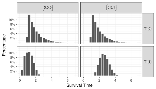
Figure 1: Histograms of ${T^{\ast}\big{(}0\big{)}}$ and ${T^{\ast}\big{(}1\big{)}}$ stratified by $X_{1}$

We compare the proposed estimator (denoted by New) with the naive estimator (denoted by Naive), which ignores censoring and pretends all observations are complete (Wang et al.,, 2018). We conduct the simulation experiment with 400 replications for sample size $n=$ 300, 500, and 1000. In this experiment, we observed that New always correctly estimates the sign of $\beta_{01}$ for both $\tau=0.25$ and $\tau=0.5$, while Naive has 4%, 2%, and 1% error rate for $n=300,500$ and $1000$ respectively in estimating the sign of $\beta_{01}$ for $\tau=0.25$ (0% error rate for $\tau=0.5$). Consideration this phenomenon, we conservatively compare the estimates for $\beta_{02}$ for the two methods in cases where $\hat{\beta}_{01}=1$. Table 2 summarizes the bias (with standard deviation in the parenthesis) of New and Naive for estimating ${\bm{\beta}}_{0}^{(\tau)}$ and $Q_{\tau}$ for different combinations of $\tau$ and $n$. To estimate $Q_{\tau}$, New plugs $\widehat{{\bm{\beta}}}_{n}$ into the formula of $\widehat{Q}_{\tau}\left(\cdot;{\widehat{G}_{C}}\right)$ in (5); and Naive does plugs-in similarly pretending all observation were complete. We observe that New has satisfactory performance, while Naive exhibits substantial bias for estimating both ${\bm{\beta}}_{0}^{(\tau)}$ and $Q_{\tau}$.

Table 1: Example 1: Parameters indexing the quantile-optimal IDRs ($\tau=0.25$ and $0.5$) in $\mathcal{D}$ and the $\tau$th quantile of the potential outcome distribution (denoted by $Q_{\tau}$), based on a Monte Carlo experiment ($n=10^{7}$).

$\tau$	${\beta}_{01}^{(\tau)}$	${\beta}_{02}^{(\tau)}$	${Q}_{0.25}$	${Q}_{0.5}$
0.25	1	-0.428	1.658	2.215
0.50	1	-0.552	1.587	2.258

Table 2: Bias (with standard deviation in the parenthesis) of New and Naive for estimating ${\bm{\beta}}_{0}^{(\tau)}$ and $Q_{\tau}$ for Example 1.

$\tau$	$n$	New			Naive
		$\beta_{02}^{(\tau)}$	$Q_{\tau}$		$\beta_{02}^{(\tau)}$	$Q_{\tau}$
0.25	300	0.005(0.066)	0.056(0.113)		-0.025(0.204)	-0.555(0.057)
	500	-0.001(0.054)	0.027(0.082)		-0.043(0.213)	-0.568(0.050)
	1000	0.001(0.043)	0.020(0.055)		-0.048(0.202)	-0.585(0.031)
0.50	300	0.002(0.098)	0.048(0.124)		0.129(0.082)	-0.618(0.078)
	500	0.003(0.080)	0.023(0.101)		0.122(0.064)	-0.617(0.065)
	1000	-0.002(0.051)	0.022(0.061)		0.134(0.051)	-0.649(0.049)

Finally, we demonstrate the smoothed resampling procedure in Section 3.3 for inference. We consider 90% and 95% confidence intervals for $\beta_{02}$ for $\tau=0.25$ and 0.5, respectively. The empirical coverage probabilities and average confidence interval lengths are reported in Table 3 for $n=1000$ based on 400 bootstrap samples. The observed empirical coverage probabilities are close to the nominal levels with reasonable lengths.

Table 3: Confidence intervals for $\beta_{02}$ using smoothed resampling

		90% CI			95% CI
$n$	$\tau$	coverage	length		coverage	length
500	$\tau=0.5$	0.89	0.17		0.92	0.21
	$\tau=0.25$	0.91	0.29		0.95	0.34
1000	$\tau=0.5$	0.88	0.13		0.93	0.16
	$\tau=0.25$	0.88	0.14		0.93	0.16

Example 2 (covariate-dependent censoring). Let ${\bm{X}}_{i}=\left(X_{i1},1,X_{i2}\right)^{T}$, where $X_{i1}$, $X_{i2}$ are independent $\mbox{Uniform}\left(0,1\right)$ random variables. The binary treatment $A_{i}$ is independent of ${\bm{X}}_{i}$ and satisfies $P(A_{i}=1)=0.5$. The distribution of censoring variable $C_{i}$ is

$$C_{i}=\begin{cases}4+\left(2-X_{i1}\right)\omega_{i},&\mbox{if }A_{i}=0\\ 2+I\left(X_{i1}<0.5\cup X_{i2}<0.5\right)+\omega_{i},&\mbox{if }A_{i}=1\end{cases},$$

where the $\omega_{i}$’s are independent $N(0,1)$ random variables. The survival time $T_{i}$ is generated by

$$T_{i}=1+X_{i1}+X_{i2}+A_{i}\left(3-3X_{i1}-1.5X_{i2}\right)+\left[0.5+A_{i}\left(1+X_{i1}+X_{i2}\right)\right]\epsilon_{i},$$ (17)

where the $\epsilon_{i}$’s are independent normal random variables with mean zero and standard deviation 0.5. The observed response is $Y_{i}=\min\left\{T_{i},C_{i}\right\}$. This configuration yields a 30% censoring rate. We consider estimating the $\tau$th quantile optimal IDR ($\tau$=0.1 and 0.25) within the class $\mathbb{D}=\big{\{}\mbox{I}\left(\beta_{1}X_{1}+\beta_{2}+\beta_{3}X_{2}>0\right):|\beta_{1}|=1,\left(\beta_{2},\beta_{3}\right)^{T}\in{\mathbb{R}^{2}}\big{\}}$. Similarly as for example 1, the parameters indexing the quantile-optimal IDRs ($\tau=0.1$ and $0.25$) and the the maximally achievable $\tau$th quantile of the potential outcome (denoted by $Q_{\tau}$) in $\mathbb{D}$ were estimated based on a large Monte Carlo experiment with sample size $n=10^{7}$ and treated as population parameter values, see Table 4.

To incorporate covariate-dependent censoring, we adopt the local Kaplan-Meier estimator (with bandwidth $h_{n}=0.08,0.1,0.12,0.14$) described in Remark 1 of Section 2 to estimate the propensity score. Table 5 summarizes the simulation results for New and Naive for $n=500$ based on 300 replications. We observe that New has satisfactory performance and its performance is stable with respect to different choices of the bandwidth $h$. In contrast, Naive exhibits substantial bias for estimating ${\bm{\beta}}_{02}^{(\tau)}$ and $Q_{\tau}$.

Table 4: Parameters indexing the quantile-optimal IDRs ($\tau=0.1$ and $0.25$) and the the maximally achievable $\tau$th quantile of the potential outcome (denoted by $Q_{\tau}$) in $\mathbb{D}$ in Example 1, based on a Monte Carlo experiment ($n=10^{7}$).

$\tau$	$\beta_{01}^{(\tau)}$	$\beta_{02}^{(\tau)}$	$\beta_{03}^{(\tau)}$	$Q_{\tau}({\bm{\beta}})$
0.10	-1	0.896	-0.774	1.853
0.25	-1	1.140	-0.825	2.247

Table 5: Bias (with standard deviation in the parenthesis) of New and Naive for estimating ${\bm{\beta}}_{0}^{(\tau)}$ and $Q_{\tau}$ for Example 2.

	$\tau=0.1$				$\tau=0.25$
Method	$\beta_{02}^{(\tau)}$	$\beta_{03}^{(\tau)}$	$Q_{\tau}$		$\beta_{02}^{(\tau)}$	$\beta_{03}^{(\tau)}$	Bias for $Q_{\tau}$
Naive	-0.107(0.150)	0.007(0.295)	-0.169(0.065)		-0.177(0.13)	0.035(0.215)	-0.206(0.048)
New ($h_{n}=0.08$)	-0.022(0.094)	0.020(0.162)	0.025(0.059)		-0.024(0.175)	-0.035(0.265)	-0.029(0.064)
New ($h_{n}=0.10$)	-0.016(0.091)	0.029(0.165)	0.030(0.058)		0.019(0.200)	-0.055(0.294)	-0.031(0.067)
New ($h_{n}=0.12$)	-0.009(0.086)	0.020(0.157)	0.027(0.058)		-0.014(0.195)	-0.046(0.277)	-0.008(0.065)
New ($h_{n}=0.14$)	-0.020(0.094)	0.035(0.170)	0.038(0.054)		0.002(0.187)	-0.029(0.275)	0.003(0.069)

Example 3 (Two-stage dynamic individualized decision rule). The simulation setup is motivated by the example in Jiang et al., 2017a . The censoring time $C\sim\mbox{Unif}\left(0,C_{0}\right)$, where $C_{0}$ is a positive constant. Let $s=1$. Generate the data up to time $s$, $\big{\{}X_{1},D_{1},\mathsf{Z}^{C}=\mbox{I}\big{(}\min\big{(}T_{1},C\big{)}>s\big{)}\big{\}},$ from the following distributions: $X_{1}\sim\mbox{Unif}\left(0,4\right)$, $D_{1}\mid X_{1}\sim\mbox{Bernoulli}(0.5)$ and $T_{1}\mid X_{1},D_{1}\sim\mbox{Exp}\big{(}\lambda_{1}(X_{1},D_{1})\big{)}$ where $\lambda_{1}(\cdot)$ is a rate function to be specified later, and $\mathsf{Z}^{C}$ is an auxiliary variable that equals the product of $\dot{R}$ and $\Gamma$ in observed data model (13).

If $\mathsf{Z}^{C}=1$, then the simulated patient is eligible for stage-two treatment. We generate the intermediate covariate $X_{2}$, second stage treatment $D_{2}$ and time $T_{2}$, representing the survival time after time $s$ according to: $e\sim\mbox{Unif}\left(0,2\right)$, $X_{2}\mid X_{1},D_{1}=0.5X_{1}-0.4\big{(}D_{1}-0.5\big{)}+e$, $D_{2}\mid X_{1},D_{1},X_{2}\sim\mbox{Bernoulli}(0.5)$, $T_{2}\mid X_{1},D_{1},X_{2},D_{2}\sim\mbox{Exp}\big{(}\lambda_{2}(X_{1},D_{1},X_{2},D_{2})\big{)}$, where $\lambda_{2}(\cdot)$ is a rate function to be specified later. For $\mathsf{Z}^{C}=1$, the observed survival time and censoring status are $Y=\min\{(s+T_{2}),C\}$ and $\Delta=\mbox{I}\{(s+T_{2})\leq C\}$, respectively; for $\mathsf{Z}^{C}=0$, the observed survival time and censoring status are $Y=\min\{T_{1},C\}$ and $\Delta=\mbox{I}\{T_{1}\leq C\}$, respectively. Let $H_{1}=\{X_{1}\}$ and $H_{2}=\{X_{1},D_{1},X_{2}\}$. For rate functions for $T_{1}$ and $T_{2}$, consider three scenarios:

1. $\lambda_{1}(H_{1},D_{1})=0.5\exp\big{(}1.75(D_{1}-0.5)(X_{1}-2)\big{)}$,
   $\lambda_{2}(H_{2},D_{2})=0.3\exp\big{(}2.5(D_{2}-0.4)(X_{2}-2)-D_{1}(X_{1}-2)\big{)}$

2. $\lambda_{1}(H_{1},D_{1})=0.2\exp\big{(}2(D_{1}-0.5)(-X_{1}+2)\big{)}$,
   $\lambda_{2}(H_{2},D_{2})=0.2\exp\big{(}1.5(D_{2}-0.5)(X_{2}-2)+0.3X_{1}+0.3X_{2}\big{)}$

3. $\lambda_{1}(H_{1},D_{1})=0.3\exp\big{(}3(D_{1}-0.3)(X_{1}-3)\big{)}$,
   $\lambda_{2}(H_{2},D_{2})=0.3\exp\big{(}2(D_{2}-0.5)(X_{2}-2)-0.5(D_{1}-0.3)(X_{1}-3)\big{)}$

For each scenario, we consider two different choice of $C_{0}$ to achieve 15% and 40% overall censoring rate, respectively.

In this setup, $T_{1}$ serves as the underlying $\sum_{j\in\{1,2\}}\mbox{I}\{D_{1}=A_{j}\}\dot{T}(A_{j},\emptyset)$ in equation (12); $T_{2}$ is the survival time after initiation of the second stage treatment conditional on $\mathsf{Z}^{C}=1$, hence $T_{2}+s$ serves as $\sum_{j\in\{1,2\},\ k\in\{1,2\}}\mbox{I}\{D_{1}=A_{j},D_{2}=B_{k}\}\dot{T}\big{(}A_{j},B_{k}\big{)}$ in (12). By the interaction between $D_{2}$ and $H_{2}$ in $\lambda_{2}(\cdot)$ functions, the three scenarios share the same true optimal second-stage strategy for patients with $\mathsf{Z}^{C}=1$, which is $d_{2}^{opt}(H_{2})=\mbox{I}(-X_{2}+2>0)$. Suppose the class of IDRs is $\mathcal{D}=\big{\{}\bm{d}_{\bm{\xi}}=(d_{1,{\bm{\beta}}},d_{2,\bm{\zeta}}):d_{1,{\bm{\beta}}}(X_{1})=\mbox{I}\{\beta_{1}X_{1}+\beta_{2}>0\},d_{2,\bm{\zeta}}(X_{2})=\mbox{I}\{\zeta_{1}X_{2}+\zeta_{2}>0\},|\beta_{1}|=1,|\zeta_{1}|=1\big{\}}$. Thus, $d_{2}^{opt}(H_{2})$ is contained in $\mathcal{D}$, and the parameter indexing $d_{2}^{opt}(H_{2})$ in $\mathcal{D}$ is ${\zeta_{01}=-1,\zeta_{02}=2}$. However, for all three cases, the true value for ${\bm{\beta}}_{0}$ indexing the optimal first-stage treatment in $\mathcal{D}$ does not have close form representations. We used grid-search with sample size $n=10^{7}$ for ${\bm{\beta}}\in\{-1\}\times[0,4]\cup\{1\}\times[-4,0]$ to obtain ${\bm{\beta}}_{0}$ in these cases, where the search space is the largest set of identifiable ${\bm{\beta}}$ since $X_{1}$ has support $[0,4]$.

With the above setup, we generate a random sample $\{X_{i1},D_{i1},Z^{C}_{i}X_{i2},Z^{C}_{i}D_{i2},Y_{i},\Delta_{i}\}$, $i=1,\ldots,n$, where $n=300,500$ and 1000 are considered. We assume the randomization probability $\pi_{1}$ and $\pi_{2}$ are known, and applied the proposed method to estimate the optimal IDR with $\tau=0.3$. Table 6 reports the simulation estimates of bias and standard deviations of the parameter indexing the quantile optimal dynamic regime $\widehat{\bm{\xi}}_{n}$. It also reports estimates of bias and standard deviation of the plug-in estimator of maximal achievable 0.3-quantile, $\widehat{Q}_{0.3}\{T^{\ast}(\bm{d}_{\widehat{\bm{\xi}}_{n}})\}$. We observe the proposed method reliably estimated the optimal two-stage IDR. The average biases and standard deviations of $\hat{\beta}_{02}$ and $\hat{\zeta}_{02}$ decrease as sample size increases. The lower censoring rate corresponds to better performance.

Table 6: Simulation Results about the bias (standard deviation of the estimates given in the parentheses) of $\widehat{\bm{\xi}}_{n}$ relative to $\bm{\xi}_{0}$ and of $\widehat{Q}_{0.3}\big{(}\widehat{\bm{\xi}}\big{)}$ relative to ${Q}_{0.3}\big{(}{\bm{\xi}_{0}}\big{)}$. We used 400 replicates. The results for $\hat{\beta}_{1}$ and $\hat{\zeta}_{1}$ were omitted, since they ought to be from the set $\{-1,1\}$ by the normalization method and our estimator correctly estimate them in each run. True value can be found in Table 7.

Case	n	C%	Bias in ${\beta}_{02}$	Bias in ${\zeta}_{02}$	Bias in ${Q}_{0.3}\big{(}{\bm{\xi}_{0}}\big{)}$
(a)	300	40	-0.052(0.499)	0.035(0.391)	0.525(0.445)
	500	40	-0.036(0.416)	0.031(0.339)	0.353(0.358)
	1000	40	-0.005(0.317)	0.043(0.282)	0.206(0.220)
	300	15	0.016(0.402)	-0.008(0.356)	0.331(0.345)
	500	15	0.010(0.329)	0.006(0.303)	0.247(0.262)
	1000	15	-0.008(0.255)	0.001(0.230)	0.139(0.187)
(b)	300	40	-0.030(0.648)	-0.023(0.371)	0.280(0.225)
	500	40	-0.031(0.581)	-0.015(0.344)	0.181(0.149)
	1000	40	-0.016(0.429)	-0.013(0.279)	0.120(0.105)
	300	15	-0.031(0.600)	0.005(0.332)	0.235(0.178)
	500	15	-0.037(0.485)	0.012(0.314)	0.155(0.137)
	1000	15	0.006(0.414)	-0.004(0.260)	0.101(0.090)
(c)	300	40	-0.084(0.433)	-0.009(0.342)	0.484(0.396)
	500	40	-0.056(0.372)	0.001(0.299)	0.380(0.347)
	1000	40	0.003(0.277)	0.008(0.250)	0.198(0.231)
	300	15	-0.074(0.404)	0.002(0.304)	0.379(0.329)
	500	15	-0.029(0.336)	-0.012(0.254)	0.261(0.286)
	1000	15	-0.015(0.249)	0.001(0.229)	0.150(0.167)

Table 7: True values of $\bm{\xi}_{0}=({\bm{\beta}}_{0}^{T},\bm{\zeta}_{0}^{T})^{T}$ indexing the 0.3 quantile-optimal DTR

	$\bm{\beta}_{0}$	$\bm{\zeta}_{0}$	$Q_{0.3}\big{(}\bm{\xi}_{0}\big{)}$
Case (a)	$\big{(}-1,2.00\big{)}^{T}$	$\big{(}-1,2\big{)}^{T}$	1.524
Case (b)	$\big{(}1,-1.95\big{)}^{T}$	$\big{(}-1,2\big{)}^{T}$	1.566
Case (c)	$\big{(}-1,2.94\big{)}^{T}$	$\big{(}-1,2\big{)}^{T}$	2.132

6 Analysis of GBSG2 study data

To illustrate the proposed method, we analyze the data from the GBSG2 study conducted by the German Breast Cancer Study Group (Schumacher et al.,, 1994; Schmoor et al.,, 1996). The study investigated the efficacy of four combinations of treatments: three versus six cycles of chemotherapy with or without the adjuvant hormonal therapy with Tamoxifen. The outcome of interest is the recurrence-free survival time in days. The dataset, available in the R package TH.data (Hothorn,, 2017), contains information on 686 patients of whom 56% had censored outcomes. The covariates include the age at diagnosis, the menopausal status, tumour size, tumour grade, the number of positive lymph nodes, estrogen receptor (ER) and progesterone receptor (PR) expression level in the tumour tissue. Earlier work on this study provided strong evidence that six cycles of chemotherapy is not superior to three cycles with respect to recurrence-free survival. Our analysis therefore focuses on IDRs regarding the assignment of adjuvant Tamoxifen therapy. Figure 2 depicts the estimated Kaplan-Meier curves for the groups of patients with and without Tamoxifen therapy.

Figure 2: Plot of the Kaplan-Meier estimator of survival functions of $T$ for $A=0,1$ respectively

First, we estimate the probability of receiving Tamoxifen. In this study, about two thirds of the recruited patients were randomized, and those who were not randomized chose the treatment by personal or professional preference. Because the randomization status is masked in the anonymous version of this data, we consider a working propensity score model by logistic regression. We observe that the randomization status is not significantly associated with the survival (Schmoor et al.,, 1996). Let $A$ denote the hormonal therapy status ($A=0$: did not receive; $A=1$: received). We first fit a logistic regression model using $A$ as the response and all available covariates. We then perform a best subset selection using the R package bestglm (McLeod and Xu,, 2010), and obtained the model $\mbox{logit}\{\pi_{A}\left({\bm{X}};\bm{\gamma}\right)\}=\gamma_{0}+\gamma_{1}\mbox{MNST}$, where MNST is the binary menopausal status of patients. Using this selected model, we obtain the estimated propensity score 0.203 for premenopausal patients, and 0.472 for postmenopausal patients. The dependency of propensity score on MNST is mostly due to a modification on the protocol for randomization starting from the third year of GBSG2 recruitment. We also tried the propensity score model with all covariates and found that it leads to almost the same recommendations as measured by the match ratio (percentage of times two decision rules make the same treatment recommendations), which is above 98% for both of the two classes of regimes under consideration.

Motivated by the extensive work in the medical literature on Tamoxifen’s molecular level mechanism and its clinical long-term effects, we consider IDRs that depend on the following three variables.

1. ER: The role of estrogen receptor expression as a predictive factor guiding the allocation of tamoxifen is well recognized. A large meta-analysis of randomized clinical trials demonstrated that high-ER patients respond better to Tamoxifen compared with low-ER patients (Group et al.,, 1998).

2. PR: Progesterone receptor expression is routinely measured for breast cancer patients as an important prognostic factor. However, its predictive power for the efficacy of Tamoxifen is still not well understood. It was observed that breast cancer patients with both high ER and high PR (‘double positive’) have the best chance of surviving (Bardou et al.,, 2003).

3. Age: Age is an important risk factor in breast cancer. We speculate that it may also contribute to how well patients respond to the adjuvant Tamoxifen therapy.

Because ER and PR are both highly skewed and have the minimal value 0 in this dataset, we adopt the transformation $\mbox{LER}=\log_{10}(\mbox{ER}+1)$ and $\mbox{LPR}=\log_{10}(\mbox{PR}+1)$. Age is linearly normalized to be between 0 and 1, and is denoted by NAGE.

We first consider the class of IDRs $\mathcal{D}_{1}$ that depend on all three variables:

$$\mathcal{D}_{1}=\big{\{}\mbox{I}\big{(}\beta_{1}\mbox{LER}+\beta_{2}+\beta_{3}\mbox{LPR}+\beta_{4}\mbox{NAGE}>0\big{)}:\beta_{1}=1,\beta_{2},\beta_{3},\beta_{4}\in\mathbb{R}\big{\}}.$$

We restrict the sign of ER to be positive based on evidence from the clinical practice (Hammond et al.,, 2010). We estimate the IDR in the class $\mathcal{D}_{1}$ that maximizes the first quartile ($\tau=0.25$) of the recurrence-free survival time. We examine the dependence of the censoring time $C$ on $A$ and all seven prognostic factors by Cox regression and conclude that the independent censoring assumption is plausible. Furthermore, since GBSG2 has a high censoring rate and relatively short follow-up time, hereafter we use the artificial censoring technique (with $M$ being set as 1550 days)in Remark 2 in Section 2.3 to improve stability of the proposed method.

Table 8: Estimated parameters indexing the quartile-optimal IDR and 90% $m$-out-of-$n$ bootstrap confidence intervals for the GBSG2 study

Regimes	$\beta_{2}$	$\beta_{3}$	$\beta_{4}$
$\mathcal{D}_{1}$	-1.23	0.94	-0.14
	(-3.39, -0.88)	(0.87, 2.02 )	(-1.21, 2.39 )
$\mathcal{D}_{2}$	-1.26	0.97	/
	(-2.41, -1.07)	(0.43, 2.01)	/

The estimated parameter indexing the quartile-optimal IDR is $\widehat{{\bm{\beta}}}_{n,\mathcal{D}_{1}}=\left(1,-1.23,0.94,-0.14\right)^{T}$. This regime leads to an estimated quartile survival time of $\widehat{Q}_{0.25}\left(\widehat{{\bm{\beta}}}_{n,\mathcal{D}_{1}}\right)=1246$ days with approximately 81.6% of patients being recommended to treatment. In contrast, the Kaplan-Meier estimator of the first quartile of the observed survival time is 727 (90% confidence interval $=(622,805)$). The first row in Table 8 reported the 90% smoothed bootstrap confidence interval (Section 3.3) for each coefficient except $\beta_{1}$ based on 400 bootstrap samples. The coefficient of NAGE, $\beta_{4}$, is insignificant at the 0.1 level, which suggests that age may not be an important variable for determining Tamoxifen.

Next, we estimate quartile-optimal IDR in the following simplified class of IDRs to obtain a concise rule,

$$\mathcal{D}_{2}=\left\{\mbox{I}\left(\beta_{1}\mbox{LER}+\beta_{2}+\beta_{3}\mbox{LPR}>0\right):\right.\left.\beta_{1}=1,\beta_{2},\beta_{3}\in\mathbb{R}\right\}.$$

The estimated parameter indexing the quartile-optimal IDR in $\mathcal{D}_{2}$ is $\widehat{{\bm{\beta}}}_{n,\mathcal{D}_{2}}=\left(1,-1.26,0.97\right)^{T}$, which leads to an estimated quartile survival time of $\widehat{Q}_{0.25}\left(\widehat{{\bm{\beta}}}_{n,\mathcal{D}_{2}}\right)=1246$ days with approximately 82.3% of patients being recommended to treatment. The second row of Table 8 reported the 90% smoothed bootstrap confidence intervals for $\beta_{2}$ and $\beta_{3}$. The coefficient for LPR is significant. Also, because the estimated $\hat{\beta}_{3}$ for LPR is about 1, we conclude that LPR is as important as the well-established predictive factor LER in developing an IDR that optimizes the first quartile survival time.

Appendix: Regularity Conditions

We introduce below a set of regularity conditions needed to establish the statistical theory. The proof of the theory is given in the online supplement.

C1

Let $L$ denote the end of the study. The censoring variable $C$ has a continuously differentiable density function which is bounded away from infinity on $\big{(}0,L\big{)}$. There exists a constant $\eta>0$ such that ${G_{C}}(L)>\eta>0$. The densities $f_{0}(t|{\bm{X}})$ and $f_{1}(t|{\bm{X}})$ are uniformly bounded away from infinity, almost surely in ${\bm{X}}$; and $\sup_{{\bm{\beta}}\in{\mathbb{B}^{o}}}{Q_{\tau}\big{\{}T^{\ast}\big{(}d_{{\bm{\beta}}}\big{)}\big{\}}}<L$. There exist positive constants $\kappa_{1}$ and $\delta$, such that $\inf_{{\bm{\beta}}\in{\mathbb{B}^{o}}}\inf_{|m-m_{0}|\leq\delta}f_{{T^{\ast}\big{(}d_{{\bm{\beta}}}\big{)}}}(m)\geq\kappa_{1}$, where $m_{0}=\sup_{{\bm{\beta}}\in{\mathbb{B}^{o}}}{Q_{\tau}\big{\{}T^{\ast}\big{(}d_{{\bm{\beta}}}\big{)}\big{\}}}$.

C2

The probability density function of $X_{1}$ conditional on $\tilde{{\bm{X}}}$ is continuously differentiable. The angular component of ${\bm{X}}$, considered as a random element of the sphere $\mathbb{S}\in\mathbb{R}^{p}$, has a bounded and continuous density.

C3

The population parameter ${\bm{\beta}}_{0}=(\beta_{01},\widetilde{{\bm{\beta}}}^{T})^{T}$ indexing the optimal IDR is unique in $\mathbb{B}^{o}$.

C4

The $(p-1)\times(p-1)$ matrix $\Lambda(\widetilde{{\bm{\beta}}},h)|_{\widetilde{{\bm{\beta}}}=\widetilde{{\bm{\beta}}}_{0},h=h_{0}},$ defined in the proof of Lemma 1 in the online supplement, is negative definite.

Remark. Condition (C1) is common in survival analysis, where $L$ is the maximum follow-up time. The survival time is not observed if it exceeds $L$. Condition (C2) has to do with population parameter identifiability, as discussed in Section 2.2. We assume after a possible rearranging of elements in ${\bm{X}}$, the density of $X_{1}$ conditional on $\tilde{{\bm{X}}}$ is continuously differentiable for every $\tilde{{\bm{X}}}$ almost surely. If all covariates are discrete, the problem of estimating an optimal IDR actually becomes simpler in some sense as there are finite many decision rules. One can directly compare the estimated value functions. Condition (C3) is standard for index models. Condition (C4) is needed for evaluating the Hessian matrix when establishing the limiting distribution of $\widehat{{\bm{\beta}}}_{n}$. See pages - of IDR_rev2_supp_names.pdf

References

- Abrevaya and Huang, (2005) Abrevaya, J. and Huang, J. (2005). On the bootstrap of the maximum score estimator. Econometrica, 73(4):1175–1204.
- Bai et al., (2017) Bai, X., Tsiatis, A. A., Lu, W., and Song, R. (2017). Optimal treatment regimes for survival endpoints using a locally-efficient doubly-robust estimator from a classification perspective. Lifetime Data Analysis, 23(4):585–604.
- Banerjee et al., (2019) Banerjee, M., Durot, C., Sen, B., et al. (2019). Divide and conquer in nonstandard problems and the super-efficiency phenomenon. The Annals of Statistics, 47(2):720–757.
- Banerjee and McKeague, (2007) Banerjee, M. and McKeague, I. W. (2007). Confidence sets for split points in decision trees. The Annals of Statistics, 35(2):543–574.
- Bardou et al., (2003) Bardou, V.-J., Arpino, G., Elledge, R. M., Osborne, C. K., and Clark, G. M. (2003). Progesterone receptor status significantly improves outcome prediction over estrogen receptor status alone for adjuvant endocrine therapy in two large breast cancer databases. Journal of Clinical Oncology, 21(10):1973–1979.
- Bickel et al., (2012) Bickel, P. J., Götze, F., and van Zwet, W. R. (2012). Resampling fewer than observations: gains, losses, and remedies for losses. In Selected works of Willem van Zwet, pages 267–297. Springer.
- Bickel and Sakov, (2008) Bickel, P. J. and Sakov, A. (2008). On the choice of m in the m out of n bootstrap and confidence bounds for extrema. Statistica Sinica, 18:967–985.
- Chakraborty et al., (2013) Chakraborty, B., Laber, E. B., and Zhao, Y. (2013). Inference for optimal dynamic treatment regimes using an adaptive m-out-of-n bootstrap scheme. Biometrics, 69(3):714–723.
- Chakraborty and Moodie, (2013) Chakraborty, B. and Moodie, E. E. (2013). Statistical Methods for Dynamic Treatment Regimes: Reinforcement Learning, Causal Inference, and Personalized Medicine. Springer Science & Business Media.
- Chakraborty et al., (2010) Chakraborty, B., Murphy, S., and Strecher, V. (2010). Inference for non-regular parameters in optimal dynamic treatment regimes. Statistical Methods in Medical Research, 19(3):317–343.
- Cui et al., (2017) Cui, Y., Zhu, R., and Kosorok, M. (2017). Tree based weighted learning for estimating individualized treatment rules with censored data. Electronic journal of statistics, 11(2):3927.
- Delgado et al., (2001) Delgado, M. A., Rodrıguez-Poo, J. M., and Wolf, M. (2001). Subsampling inference in cube root asymptotics with an application to manski’s maximum score estimator. Economics Letters, 73(2):241–250.
- Delsol and Van Keilegom, (2020) Delsol, L. and Van Keilegom, I. (2020). Semiparametric m-estimation with non-smooth criterion functions. Annals of the Institute of Statistical Mathematics, 72(2):577–605.
- Díaz et al., (2018) Díaz, I., Savenkov, O., and Ballman, K. (2018). Targeted learning ensembles for optimal individualized treatment rules with time-to-event outcomes. Biometrika, 105(3):723–738.
- Goldberg and Kosorok, (2012) Goldberg, Y. and Kosorok, M. R. (2012). Q-learning with censored data. Annals of Statistics, 40(1):529.
- Gonzalez-Manteiga and Cadarso-Suarez, (1994) Gonzalez-Manteiga, W. and Cadarso-Suarez, C. (1994). Asymptotic properties of a generalized kaplan-meier estimator with some applications. Communications in Statistics-Theory and Methods, 4(1):65–78.
- Group et al., (1998) Group, E. B. C. T. C. et al. (1998). Tamoxifen for early breast cancer: an overview of the randomised trials. The Lancet, 351(9114):1451–1467.
- Hager et al., (2018) Hager, R., Tsiatis, A. A., and Davidian, M. (2018). Optimal two-stage dynamic treatment regimes from a classification perspective with censored survival data. Biometrics, 74(4):1180–1192.
- Hammond et al., (2010) Hammond, M. E. H., Hayes, D. F., Dowsett, M., Allred, D. C., Hagerty, K. L., Badve, S., Fitzgibbons, P. L., Francis, G., Goldstein, N. S., Hayes, M., et al. (2010). American society of clinical oncology/college of american pathologists guideline recommendations for immunohistochemical testing of estrogen and progesterone receptors in breast cancer (unabridged version). Archives of Pathology & Laboratory Medicine, 134(7):e48–e72.
- Hothorn, (2017) Hothorn, T. (2017). TH.data: TH’s Data Archive. https://cran.r-project.org/web/packages/TH.data/.
- (21) Jiang, R., Lu, W., Song, R., and Davidian, M. (2017a). On estimation of optimal treatment regimes for maximizing t-year survival probability. Journal of the Royal Statistical Society: Series B, 79(4):1165–1185.
- (22) Jiang, R., Lu, W., Song, R., Hudgens, M. G., Naprvavnik, S., et al. (2017b). Doubly robust estimation of optimal treatment regimes for survival data with application to an hiv/aids study. The Annals of Applied Statistics, 11(3):1763–1786.
- Kim and Pollard, (1990) Kim, J. K. and Pollard, D. (1990). Cube root asymptotics. The Annals of Statistics, 18:191–219.
- Koenker, (2005) Koenker, R. (2005). Quantile Regression. Cambridge University Press.
- Kosorok, (2008) Kosorok, M. R. (2008). Introduction to Empirical Processes and Semiparametric Inference. Springer, New York.
- Kosorok and Moodie, (2016) Kosorok, M. R. and Moodie, E. E. (2016). Adaptive Treatment Strategies in Practice: Planning Trials and Analyzing Data for Personalized Medicine. ASA-SIAM Series on Statistics and Applied Probability, SIAM, Philadelphia, ASA, Alexandria, VA.
- Laber and Zhao, (2015) Laber, E. and Zhao, Y. (2015). Tree-based methods for individualized treatment regimes. Biometrika, 102(3):501–514.
- Lavori and Dawson, (2000) Lavori, P. W. and Dawson, R. (2000). A design for testing clinical strategies: biased adaptive within-subject randomization. Journal of the Royal Statistical Society: Series A, 163:29–38.
- Léger and MacGibbon, (2006) Léger, C. and MacGibbon, B. (2006). On the bootstrap in cube root asymptotics. Canadian Journal of Statistics, 34(1):29–44.
- Luedtke and van der Laan, (2016) Luedtke, A. and van der Laan, M. J. (2016). Statistical inference for the mean outcome under a possibly non-unique optimal treatment strategy. The Annals of Statistics, 44(2):713–742.
- Matsouaka et al., (2014) Matsouaka, R. A., Li, J., and Cai, T. (2014). Evaluating marker-guided treatment selection strategies. Biometrics, 70(3):489–499.
- McLeod and Xu, (2010) McLeod, A. and Xu, C. (2010). bestglm: Best subset glm. https://cran.r-project.org/web/packages/bestglm/.
- Mebane Jr and Sekhon, (2011) Mebane Jr, W. R. and Sekhon, J. S. (2011). Genetic optimization using derivatives: the rgenoud package for r. Journal of Statistical Software, 42:1–26.
- Mitchell, (1998) Mitchell, M. (1998). An Introduction to Genetic Algorithms. MIT press.
- Moodie and Richardson, (2010) Moodie, E. E. and Richardson, T. S. (2010). Estimating optimal dynamic regimes: Correcting bias under the null. Scandinavian Journal of Statistics, 37(1):126–146.
- Murphy, (2003) Murphy, S. A. (2003). Optimal dynamic treatment regimes. Journal of the Royal Statistical Society: Series B, 65(2):331–366.
- (37) Murphy, S. A. (2005a). An experimental design for the development of adaptive treatment strategies. Statistics in medicine, 24(10):1455–1481.
- (38) Murphy, S. A. (2005b). A generalization error for q-learning. Journal of Machine Learning Research, 6:1073–1097.
- Murphy, (2008) Murphy, S. A. (2008). An experimental design for the development of adaptive treatment strategies. Statistics in Medicine, 24:1455–1481.
- Neyman, (1923) Neyman, J. (1923). Sur les applications de la théorie des probabilités aux experiences agricoles: Essai des principes. Roczniki Nauk Rolniczych, 10:1–51.
- Orellana and Robins, (2010) Orellana, L., R. A. and Robins, J. (2010). Dynamic regime marginal structural mean models for estimation of optimal dynamic treatment regimes, part i: Main content. The International Journal of Biostatistics, 6.
- Patra et al., (2018) Patra, R. K., Seijo, E., and Sen, B. (2018). A consistent bootstrap procedure for the maximum score estimator. Journal of Econometrics, 205(2):488–507.
- Qian et al., (2021) Qian, M., Chakraborty, B., Maiti, R., and Cheung, Y. K. (2021). A sequential significance test for treatment by covariate interactions. Statistica Sinica. In press.
- Qian and Murphy, (2011) Qian, M. and Murphy, S. A. (2011). Performance guarantees for individualized treatment rules. The Annals of Statistics, 39(2):1180–1210.
- Robins et al., (2000) Robins, J., Hernan, M., and Brumback, B. (2000). Marginal structural models and causal inference in epidemiology. Epidemiology, 11:550–560.
- Robins and Rotnitzky, (2014) Robins, J. and Rotnitzky, A. G. (2014). Discussion of “dynamic treatment regimes: Technical challenges and applications”. Electronic Journal of Statistics, 8:1273–1289.
- Robins and Rotnitzky, (2008) Robins, J.M., O. L. and Rotnitzky, A. (2008). Estimation and extrapolation of optimal treatment and testing strategies. Statistics in Medicine, 27:4678–4721.
- Rosenbaum and Rubin, (1983) Rosenbaum, P. R. and Rubin, D. B. (1983). The central role of the propensity score in observational studies for causal effects. Biometrika, 70:41–55.
- Rubin, (1978) Rubin, D. B. (1978). Bayesian inference for causal effects: The role of randomization. The Annals of statistics, 6(1):34–58.
- Rubin, (1986) Rubin, D. B. (1986). Which ifs have causal answers. Journal of the American Statistical Association, 81:961–962.
- Schmoor et al., (1996) Schmoor, C., Olschewski, M., and Schumacher, M. (1996). Randomized and non-randomized patients in clinical trials: experiences with comprehensive cohort studies. Statistics in Medicine, 15(3):263–271.
- Schumacher et al., (1994) Schumacher, M., Bastert, G., Bojar, H., Huebner, K., Olschewski, M., Sauerbrei, W., Schmoor, C., Beyerle, C., Neumann, R., and Rauschecker, H. (1994). Randomized 2 x 2 trial evaluating hormonal treatment and the duration of chemotherapy in node-positive breast cancer patients. german breast cancer study group. Journal of Clinical Oncology, 12(10):2086–2093.
- Sen et al., (2010) Sen, B., Banerjee, M., Woodroofe, M., et al. (2010). Inconsistency of bootstrap: The grenander estimator. The Annals of Statistics, 38(4):1953–1977.
- Shi et al., (2018) Shi, C., Lu, W., and Song, R. (2018). A massive data framework for m-estimators with cubic-rate. Journal of the American Statistical Association, 113(524):1698–1709.
- Simoneau et al., (2020) Simoneau, G., Moodie, E. E., Nijjar, J. S., Platt, R. W., Investigators, S. E. R. A. I. C., et al. (2020). Estimating optimal dynamic treatment regimes with survival outcomes. Journal of the American Statistical Association, 115:1531–1539.
- Song et al., (2015) Song, R., Wang, W., Zeng, D., and Kosorok, M. (2015). Penalized q-learning for dynamic treatment regimens. Statistica Sinica, 25:901–920.
- van der Vaart and Wellner, (1996) van der Vaart, A. W. and Wellner, J. A. (1996). Weak Convergence and Empirical Processes with Applications to Statistics. Springer-Verlag, New York.
- Wahed, (2009) Wahed, A. S. (2009). Estimation of survival quantiles in two-stage randomization designs. Journal of Statistical Planning and Inference, 139(6):2064–2075.
- Wang et al., (2018) Wang, L., Zhou, Y., Song, R., and Sherwood, B. (2018). Quantile-optimal treatment regimes. Journal of the American Statistical Association, 113(523):1243–1254.
- Watkins and Dayan, (1992) Watkins, C. and Dayan, P. (1992). Q-learning. Machine Learning, 8:279–292.
- Wu and Wang, (2021) Wu, Y. and Wang, L. (2021). Resampling-based confidence intervals for model-free robust inference on optimal treatment regimes. Biometrics, 77(2):465–476.
- Xu et al., (2016) Xu, Y., Müller, P., Wahed, A. S., and Thall, P. F. (2016). Bayesian nonparametric estimation for dynamic treatment regimes with sequential transition times. Journal of the American Statistical Association, 111(515):921–950.
- Zhang et al., (2012) Zhang, B., Tsiatis, A. A., Laber, E. B., and Davidian, M. (2012). A robust method for estimating optimal treatment regimes. Biometrics, 68(4):1010–1018.
- Zhang et al., (2018) Zhang, Y., Laber, E., Davidian, M., and Tsiatis, A. (2018). Estimation of optimal treatment regimes using lists. 113:1541–1549.
- (65) Zhao, Y., Zeng, D., Laber, E. B., Song, R., Yuan, M., and Kosorok, M. R. (2015a). Doubly robust learning for estimating individualized treatment with censored data. Biometrika, 102(1):151–168.
- Zhao et al., (2012) Zhao, Y., Zeng, D., Rush, A. J., and Kosorok, M. R. (2012). Estimating individualized treatment rules using outcome weighted learning. Journal of the American Statistical Association, 107(499):1106–1118.
- (67) Zhao, Y. Q., Zeng, D., Laber, E. B., and Kosorok, M. R. (2015b). New statistical learning methods for estimating optimal dynamic treatment regimes. Journal of the American Statistical Association, 110:583–598.
- Zhou, (2006) Zhou, L. (2006). A simple censored median regression estimator. Statistica Sinica, 16(3):1043–1058.
- Zhu et al., (2017) Zhu, R., Zhao, Y.-Q., Chen, G., Ma, S., and Zhao, H. (2017). Greedy outcome weighted tree learning of optimal personalized treatment rules. Biometrics, 73(2):391–400.