A study of 1000 galaxies with unusually young and massive stars in the SDSS: a search for hidden black holes

Abstract

We select 1076 galaxies with extinction-corrected H$\alpha$ equivalent widths too large to be explained with a Kroupa (2001) IMF, and compare these with a control sample of galaxies that is matched in stellar mass, redshift and 4000 Å break strength, but with normal H$\alpha$ equivalent widths. Our goal is to study how processes such as black hole growth and energetic feedback processes from massive stars differ between galaxies with extreme central H$\alpha$ emission and galaxies with normal young central stellar populations. The stellar mass distribution of H$\alpha$ excess galaxies is peaked at $3\times 10^{10}M_{\odot}$ and almost all fall well within the star-forming locus in the [OIII]/H$\beta$ versus [NII]/H$\alpha$ BPT disgram. H$\alpha$ excess galaxies are twice as likely to exhibit H$\alpha$ line asymmetries and 1.55 times more likely to be detected at 1 GHz in the VLA FIRST survey compared to control sample galaxies. The radio luminosity per unit stellar mass decreases with the stellar age of the system. Using stacked spectra, we demonstrate that [NeV] emission is not present in the very youngest of the radio-quiet H$\alpha$ excess galaxies with detectable Wolf-Rayet features, suggesting that black hole growth has not yet commenced in such systems. [NeV] emission is detected in H$\alpha$ excess galaxies with radio detections and the strength of the line correlates with the radio luminosity. This is the clearest indication for a population of black holes that may be forming in a subset of the H$\alpha$ excess population.

1 Introduction

The majority of accreting black holes identified through their UV/optical emission appear to be accreting at sub-Eddington rates, both in the local Universe (Kauffmann & Heckman 2009) and at redshifts $z$=1-2 (Aird et al 2011). The existence of very luminous quasars at $z\sim 6-7$ that are likely powered by accretion onto black holes of masses of at least $10^{9}M_{\odot}$ (Fan et al 2003) implies a separate channel of “seed” black hole formation in the early Universe (Volonteri 2010) to allow black holes to reach very high masses less than a gigayear after the Big Bang.

The physics governing the formation of seed black holes is still highly speculative. Many theoretical models have been presented in the literature with varying assumptions and complexity. The models generally fall into two categories: 1) direct collapse of low angular momentum gas clouds (e.g. Loeb & Rasio (1994), Bromm & Loeb (2003), Begelman, Volonteri & Rees (2006), Lodato & Natarajan (2006,), 2) mergers and accretion in dense stellar clusters (e.g. Portegies Zwart et al 2004, Devecchi & Volonteri 2009).

Most observational work has focused on detecting a remnant population of seed black holes of masses $10^{4}-10^{6}M_{\odot}$ (often termed imtermediate mass black holes – IMBHs for short) in present-day galaxies (see Mezcua 2017 for a detailed review). There have been observational campaigns focused on the detection of IMBHs through stellar kinematic studies of globular clusters, or via signatures of gas accretion at X-ray wavelengths in nearby galaxies.

Much recent activity has also been devoted to identifying subsets of dwarf galaxies that are likely to harbour low mass black holes. Out of a sample of 44,594 galaxies with stellar masses less than $3\times 10^{9}M_{\odot}$ in the Sloan Digital Sky Survey, Reines et al (2013) identify a subsample of 151 galaxies with emission line spectra indicative of ionization by an AGN (i.e 0.3 % of the parent sample). Twenty-five of these objects exhibit broad emission lines, and the width of these lines, together with the assumption that the ionized gas is in virial equilibrium within the potential well of the black hole, provide upper limits on the black hole masses of $\sim 10^{5}M_{\odot}$. The detection of hard X-ray emission spatially coincident with core radio emission in a subset of these dwarf galaxies (Reines et al. 2011, 2016; Reines & Deller 2012; Baldassare et al. 2015) provides futher strong evidence for the existence of accreting black holes in these systems.

Observational studies that focus on identifying IMBHs in the local galaxy population do not necessarily shed light on the processes by which they formed. The majority of present-day galaxies are relatively quiescent and processes such as gas accretion or runaway stellar mergers that formed the IMBHs may have occurred quite far in the past. We note however that follow-up observations of one of the brightest known ultra-luminous X-ray sources ESO 243-49 HLX-1 in the SOa galaxy ESO 243-49 revealed the presence of a surrounding young stellar population of age $\sim$13 Myr (Farrell et al 2012).

Another possible route to studying the formation of IMBHs is to search for evidence of accreting black holes in young star clusters. Motivated by evidence that the stars near the Milky Way’s center have IMFs with an excess of massive stars (e.g. Lu et al 2013, Hosek et al 2019), Kauffmann (2021) carried out a search for galaxies in the range $10^{10}-10^{11}M_{\odot}$ with central stellar populations indicative of an initial mass function (IMF) flatter than Salpeter at high stellar masses. 15 face-on galaxies with stellar masses in the range $10^{10}-10^{11}M_{\odot}$ were identified in the 2nd public data release of the Mapping Nearby Galaxies at APO (MaNGA) survey (Bundy et al 2015) where the 4000 Å break was either flat or rising towards the centre of the galaxy, indicating that the central regions host evolved stars, but where the H$\alpha$ equivalent width was also steeply rising to extremely high values in the central regions. The ionization parameter was low in these unusual Galactic Centres, indicating that ionizing sources were primarily stellar rather than AGN. Wolf-Rayet features characteristic of hot young stars were also often found in the spectra and these tended to get progressively stronger at smaller galactocentric radii. Finally, a large fraction of these objects (8 out of 15) were detected at radio wavelengths.

There are a number of other suggestions from observations that the stellar initial mass function (IMF) in environments with high stellar densities may differ from the canonical Kroupa (2001) IMF. Globular clusters in the Andromeda galaxy exhibit a trend between metallicity and mass-to-light ratio that only a non-canonical, top-heavy IMF could explain (Haghi et al. 2017) and ultra-compact dwarf galaxies have large dynamical mass-to-light ratios and appear to contain an overabundance of luminous X-ray binary sources (Dabringhausen et al. 2009). As pointed out in a recent theoretical paper by Weatherford et al. (2021), star clusters that have formed with a top heavy IMF are expected not only to produce more black holes, but also to produce many more binary black hole mergers and intermediate mass black holes. Natarajan (2021) also point out that gas accretion during the initial formation of the cluster can lead to extremely rapid growth, scaling a stellar mass remnant seed black hole up to intermediate mass black hole range. If the star-forming bulge already contains a pre-existing central supermassive black hole, its mass is also likely to be growing significantly if surrounded by starburst with a top-heavy IMF.

Kauffmann (2021) highlighted one galaxy out of the sample of 15 as a possible candidate for a “transition” object with a black hole in the process of formation or rapid new growth. This galaxy is among those with the strongest Wolf Rayet signatures. It was unusual in that it showed the strongest Wolf-Rayet signatures, significant central HeII$\lambda$4686 emission and clear non-Gaussian H$\alpha$ profiles in the centre of the galaxy.

In this paper, we return to the full sample of galaxies with single-fibre spectroscopy from Sloan Digital Sky Survey observations. We select all galaxies with extinction-corrected H$\alpha$ equivalent widths well above the range that can be explained with a Kroupa (2001) IMF, and compare these objects with a control sample of galaxies that is exactly matched in stellar mass, redshift and 4000 Å break strength, but with “normal” H$\alpha$ equivalent widths. Our goal is to use the much larger samples to investigate more systematically how processes such as black hole growth and energetic feedback processes from massive stars may differ between galaxies with extremely strong central H$\alpha$ emission and galaxies with “normal” young central stellar populations. We also use stacked spectra to investigate the presence of “hidden” AGN in galaxies where the strongest emission lines are dominated by emission from HII regions.

In section 2, we describe the selection of the two samples and discuss their distributions of physical properties such as stellar mass, $r$-band light concentration index, mean stellar age, and their locations in the Baldwin, Philipps & Terlevich (1981) (BPT) emission line ratio diagrams. We also present the quantities that are measured directly from the galaxy spectra. In section 3, we analyze non-Gaussian H$\alpha$ line profiles, blue and red bump Wolf Rayet features in the two samples, as well as correlations between these quantities and the global properties of the host galaxies. A cross-match with the VLA FIRST catalogue (Condon et al 1998) allows us to analyze the radio properties of the samples. In section 4, we analyze stacked spectra constructed from H$\alpha$ excess galaxies with radio and Wolf Rayet feature detections. In section 5, we summarize our results and discuss the future prospects of this work.

2 Sample selection and derived quantities

We begin with two publically-available value-added galaxy catalogues distributed through the SDSS Science Archive Server (SAS). The first is the Wisconsin catalogue of PCA-Based Stellar Masses and Velocity Dispersions (Chen et al 2012), which contains estimates of star formation history parameters (mean stellar age and burst mass fraction), metallicity, dust extinction and velocity dispersion, based on a library of model spectra for which principal components have been identified. In this paper, we make use of the stellar masses and mean stellar ages estimated using Bruzual & Charlot (2003) stellar population synthesis models with a Kroupa (2001) IMF to generate the principal components.

The second is the catalogue of Portsmouth Stellar Kinematics and Emission Line Fluxes (Thomas et al 2013). The Penalized PiXel Fitting (pPXF, Cappellari & Emsellem 2004) and Gas and Absorption Line Fitting code (GANDALF v1.5; Sarzi et al. 2006) is used to calculate stellar kinematics and to derive the emission line properties of galaxies. The stellar population models from Maraston & Strömbäck (2011) based on the MILES stellar library (Sánchez-Blázquez et al. 2006), augmented with theoretical spectra at wavelengths $<$ 3500 Å  from Maraston et al. (2009), based on the theoretical library UVBLUE (Rodríguez-Merino et al. 2005) are adopted as templates for stellar continuum fitting. In this paper, we make use of the H$\alpha$ flux and equivalent width measurements, as well as the strong line fluxes H$\beta$, [OIII]$\lambda$5007 and [NII]$\lambda$6584 to examine the location of galaxies in the standard BPT line diagnostic diagram.

We select two galaxy samples on the basis of their H$\alpha$ equivalent widths. Following the procedure adopted in Kauffmann (2021), when calculating the H$\alpha$ equivalent width, the H$\alpha$ line flux is corrected for dust attenuation using the measured Balmer decrement using the formula $A_{V}=1.9655R_{V}\log(H\alpha/H\beta/2.87)$, where $R_{V}=3.1$ and the Calzetti (2001) attenuation curve has been adopted. The stellar continuum measurements are not corrected for dust attenuation. This simplifying assumption is motivated by the finding by Wild et al (2011) that there is a strong increase in emission-line-to-continuum dust attenuation with the specific star formation rate of the galaxy. The samples are limited in redshifts to $z<0.37$ to ensure that H$\alpha$ lies well within the wavelength range where secure measurements of the H$\alpha$ equivalent width are possible, and to galaxies with $M_{*}>10^{9}M_{\odot}$.

The first sample is selected to have EQW(H$\alpha$/Å)$>800$. As shown in Kauffmann et al (2201), this is the maximum H$\alpha$ equivalent achievable for a single stellar population of age $\sim 10^{6}$ yr. This sample is termed the H$\alpha$ excess sample and consists of 1076 galaxies selected out of a total of 857493 galaxies in the same redshift and stellar mass range (i.e. 0.125% of the parent sample). The second sample is selected to have $80<$EQW(H$\alpha$/Å)$<300$ and consists of 10710 galaxies. In Figure 1, red and blue histograms show how this samples and the H$\alpha$ excess sample are distributed as a function of a variety of different quantities. These include 1)stellar mass $M_{*}$, 2)redshift, 3)4000 Å break strength (we use the narrow definition in Balogh et al (1999), which we term D_n(4000)), 4)mean stellar age, 5)concentration index of the $r$-band light, defined as the ratio of the aperture enclosing 90% of the total light to the aperture enclosing 50% of the light, 6)half-light radius of the galaxy in arcsecond, 7)Balmer decrement H$\alpha$/H$\beta$, and 8)the two BPT line ratios [OIII]/H$\beta$ and [NII]/H$\alpha$.

The H$\alpha$ excess sample shown by red histograms is clearly offset to higher stellar masses, redshifts and Balmer decrement values compared to the sample with normal H$\alpha$ EQW values, shown by blue histograms. Interestingly, the stellar mass distribution of the H$\alpha$ excess sample peaks at $\log(M_{*}/M_{\odot})\sim 10.5$, which is the mass where the galaxy population transitions from predominantly star-forming to predominantly passive, with little ongoing star formation (Kauffmann et al 2003a). Only 25% of the H$\alpha$ excess sample have stellar masses less than $10^{10}M_{\odot}$ compared to 60% of the sample with lower H$\alpha$ equivalent widths. This shows that the H$\alpha$ excess phenomenon is not confined to low mass galaxies. The median redshift of the galaxies in the H$\alpha$ excess sample is $\sim 0.2$ and the galaxies typically have half-light radii less than 2 arcseconds. The SDSS fiber diameter is 1.5”. In very low redshift galaxies, it will sample light mainly from the inner bulge, but this is not the case for the galaxies under study here. We note that the median redshift of the sample studied by Kauffmann (2021) was 0.05. We will come back to the implications of the mismatch in physical scales for the interpretation of the results in this paper in the final discussion section of this paper.

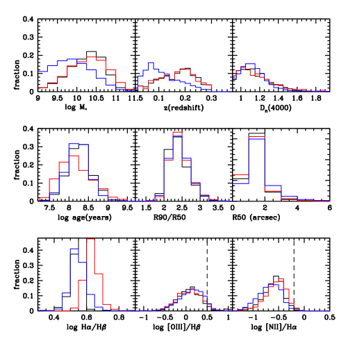
Figure 1: Red and black histograms show how the H$\alpha$ excess and control samples are distributed as a function of stellar mass $M_{*}$, redshift, 4000 Å break strength, mean stellar age, $r$-band concentration index, half-light radius in arcseconds, Balmer decrement and the two BPT line ratios [OIII]/H$\beta$ and [NII]/H$\alpha$. Blue histograms show the distribution for the full sample with 80$<$ EQW(H$\alpha$/Å)$<$300 (i.e. before matching by stellar mass, redshift and D_n(4000))

Table 1: Table of catalog quantities for the H$\alpha$ excess sample. The columns are as follows: 1) SDSS identifier, Plate ID, 2) SDSS identifier, MJD, 3) SDSS indentifier, fibre ID, 4) right ascension (J2000), 5) declination (J2000), 6) redshift, 7) logarithm of the stellar mass (M_⊙), 8) 4000 Å  break (narrow definition), 9) logarithm of the stellar age (years), 10) H$\alpha$ equivalent width, 11) H$\alpha$ equivalent width (extinction corrected), 12) log H$\alpha$/H$\beta$, 13) log [OIII]/H$\beta$, 14)log [NII]/H$\alpha$

plate id	mjd	fibre id	RA	DEC	z	log M∗	Dn(4000)	log age	EQW(H$\alpha$)	EQW(H$\alpha_{c}$)	log H$\alpha$/H$\beta$	log [OIII]/H$\beta$	log [NII]/H$\alpha$
266	51602	521	146.386	1.147	0.270	10.246	1.080	8.614	227.77	1249.76	3.941	-9.000	-0.832
267	51608	493	148.146	0.249	0.082	10.400	1.371	8.618	140.73	1223.52	4.299	0.105	-0.535
270	51909	224	152.409	-0.160	0.138	10.059	1.005	7.885	150.51	816.37	3.933	0.273	-0.604

We have also created a matched control sample by selecting galaxies from the lower EQW(H$\alpha$) sample so that the two samples match in stellar mass, redshift and 4000 Å break strength. This sample is shown as a black histogram in Figure 1. As can be seen, a larger fraction of the H$\alpha$ excess sample has mean stellar ages less than $10^{8}$ years compared to the control sample. The H$\alpha$ excess sample also has higher Balmer decrements, but has similar morphological parameters and BPT line ratio distributions compared to the control sample. Figure 2 shows the location of the galaxies in the H$\alpha$ excess and control samples in the two-dimensional [OIII]/H$\beta$ versus [NII]/H$\alpha$ BPT diagrams. As can be seen, almost all the galaxies in both samples fall below the Kauffmann et al (2003b) demarcation between star-forming galaxies and AGN/composite systems and none fall in the region of the diagram occupied by Seyferts or LINERs. The excitation of the strong emission lines in both samples appears to be radiation from young stars. Figure 3 shows the location of both samples in the plane of mean stellar age versus stellar mass. Mean stellar age increases with stellar mass in both samples. Galaxies with stellar masses of $\sim 10^{9}M_{\odot}$ have mean stellar ages of a few $\times 10^{7}M_{\odot}$, increasing to a few $\times 10^{8}M_{\odot}$ at a stellar mass of $\sim 10^{11}M_{\odot}$. The relation is somewhat steeper for the H$\alpha$ excess sample, but the differences between the relations for the two samples are quite small, suggesting that the two samples may be indicative of different phases of a single type of starburst. Note that all references to the control sample from now on, refer to the sample that is matched in stellar mass, redshift and 4000 Å break strength. Table 1 provides a list of catalogue quantities for all galaxies in the H$\alpha$ excess sample. A corresponding table for the control sample galaxies is also provided as part of the online supplementary material that accompanies this paper.

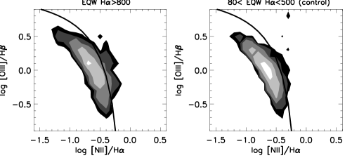
Figure 2: Location of the H$\alpha$ excess sample (left) and control sample (right) in the [OIII]/H$\beta$ versus [NII]/H$\alpha$ BPT diagrams. The solid curve shows the Kauffmann et al (2003b) demarcation between star-forming galaxies and AGN/composite systems.

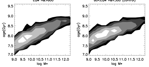
Figure 3: Location of the H$\alpha$ excess sample (left) and control sample (right) in the plane of mean stellar age versus stellar mass.

2.1 H$\alpha$ line profile analysis

By construction, the H$\alpha$ line in the spectra of the galaxies in both samples is always very strong and hence amenable to a detailed line profile analysis. Most of the standard SDSS spectral pipelines fit simple Gaussian profiles to a list of strong emission lines after subtracting a linear combination of template spectra that provides the best fit to the stellar continuum over the wavelength interval from $\sim$3500 to $\sim$7000 Å. In this analysis, we look at the deviations of the observed spectrum from the best single Gaussian fit.

We extract the observed and the best-fit model spectra obtained using the FIREFLY code (Wilkinson et al. 2017; Comparat et al 2017) for the galaxies in the H$\alpha$ excess and control samples. The left panels in Figure 4 show three example spectra plotted over the wavelength range from 6530 to 6600 Å, which includes the H$\alpha$ line at 6563 Å, as well as the [NII] lines at 6584 and 6548 Å. The right panels show the spectra after subtraction of the FIREFLY continuum fit. We first fit the two [NII] lines over the wavelength range shown as red curves in each panel. The width of the weaker 6548 Å line is fixed to be the same as that of the 6584 Å  line. The best-fit single Gaussian profiles are subtracted and we then fit the H$\alpha$ line. The best single Gaussian fit is shown in cyan in each panel in the right column of the plot. The results shown in the top right panel indicate that a good fit to H$\alpha$ is obtained with a single Gaussian. The fits shown in the middle and bottom right panels reveal significant residual flux away from the line centre. In the middle right panel, the residual flux is found redwards of the H$\alpha$ line centroid and in the bottom right panel, residual flux is found on both sides of the line.

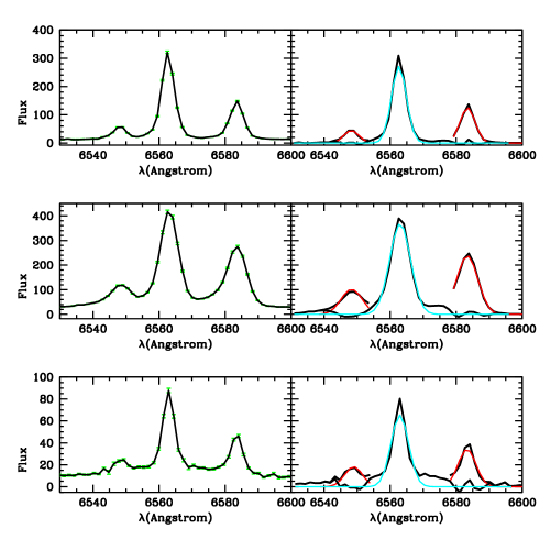
Figure 4: Three example spectra plotted over the wavelength range from 6530 to 6600 Å. The left panels show the observed spectrum in black with errors indicated as green errorbars. In the right panels, the black curves show the spectra after subtraction of the FIREFLY continuum fit. The two [NII] lines are fit over the wavelength range shown as red curves in each panel.The best single Gaussian fit to the H$\alpha$ line after subtracting the Gaussian fits to the two [NII] lines is shown in cyan in each panel.

We calculate the summed residual flux as the sum of the difference between the observed flux and the single Gaussian model fit over each spectral bin. The residuals are calculated separately on the red and blue side of the line centroids. If a positive summed residual flux is detected with a $S/N$ greater than 5 on either the blue or the red side of the H$\alpha$ line centroids, we classify the galaxy as having an H$\alpha$ asymmetry. We calculate $V_{80}({\rm blue})$ and $V_{80}({\rm red})$ in units of km/s by measuring the wavelength difference between the centroid of the single Gaussian fit to the H$\alpha$ line and the wavelength enclosing 80% of the summed residual flux on both sides of the line centre.

We note that our procedure differs from that used in other studies (e.g. Förster-Schreiber et al 2019), who fit three broad Gaussian components to H$\alpha$ and the two [NII] lines. Their sample includes many classical AGN with high [NII]/H$\alpha$ ratios, whereas the [NII] lines are always relatively weak in comparison to H$\alpha$ in our samples. In our sample, it is reasonable to ascribe the bulk of the detected residual flux to the H$\alpha$ line. We have also checked our single-Gaussian fits to the [OIII] lines and we almost never find excess flux at large velocity separations, suggesting that the gas that we detect at large separation is cool. Finally, as we show in section 4, the high velocity gas traced by H$\alpha$ is found in conjunction with significant shifts in the Na I $\lambda\lambda$ 5890, 5896 (Na D) absorption lines with respect to galaxies that do not exhibit H$\alpha$ line profile asymmteries. The NaD absorption lines are believed to trace the neutral gas component of galaxies (Heckman & Lehnert 2000).

Finally, we note that the H$\alpha$ line fitting procedure is not applied to galaxies where more than 10% of the spectral bins over the wavelength range shown in Figure 4 are flagged as problematic. This reduces the size of the analyzed sample from 1076 to 340 galaxies located at lower redshifts where contamination by sky lines are less severe.

2.2 Identification of Wolf-Rayet Features

The procedure we adopt is similar to that described in Brinchmann, Kunth & Durret (2008). We adopt the continuum and central bandpass definitions for the blue and red Wolf-Rayet features given in Table 1 of this paper. The central passband used to probe the blue feature extends over the wavelength range 4655-4755 Å. This definition assumes that the blue Wolf Rayet feature is dominated by broad HeII$\lambda$4686 from WN stars and [FeIII]$\lambda$4658 from O stars and that the WC stars that contribute to CIII $\lambda$4650 at the edge of the blue central band are sub-dominant. The red feature central bandpass assumes that it is dominated by CIV $\lambda$5808 from early WC stars, rather than CIII $\lambda$5696 which dominates in late WC stars and forms part of the continuum band. The definitions are optimized for metal poor populations where WN stars dominate over WC stars and where early WC stars are relatively common and late WC stars are rare/absent. We will discuss the limitations of, and possible changes to, this approach in the final section of the paper.

Because the galaxy spectra are quite complex over the wavelength range of the blue and red bump features, we rescale the FIREFLY stellar continuum model fits so that the average flux computed in the two continuum bands in the observed spectra and in the model fits match exactly. Unlike Brinchmann et al, we do not attempt to fit indivdual lines within the central bandpass – instead, we define an integrated equivalent width for the summed flux over the full wavelength range. This allows us to calculate the error on the Wolf Rayet “bump” detection in a much more straightforward way. We select all galaxies with a positive equivalent width measurement with a signal-to-noise greater than 3 as Wolf-Rayet galaxy candidates. Because the features are weak in most of the galaxies, the analysis in this paper will focus on the analysis of stacked spectra of subsets of these candidates.

In Figure 5, we plot examples of three blue bump Wolf Rayet candidates from the H$\alpha$ excess sample where the central bandpass excess is detected with $S/N>10$. In the plot, the central bandpass is delineated by blue lines and the two continuum bandpasses by red lines. In the bottom panel, we plot the stacked spectrum of all the blue bump Wolf Rayet candidates. Only in the stacked spectrum is the broadened HeII line at 4686 Å clearly visible. There is also a weak NIII$\lambda$4640 line visible in the stacked spectrum. We return to a discussion of this in section 3.2. Although our methodology does pick up some red bump Wolf Rayet candidates (Figure 6), individual emission lines cannot be distinguished within the red bump window even in the stack. In particular the CIV$\lambda$5808 line is not clearly detected even in the stacked spectrum.

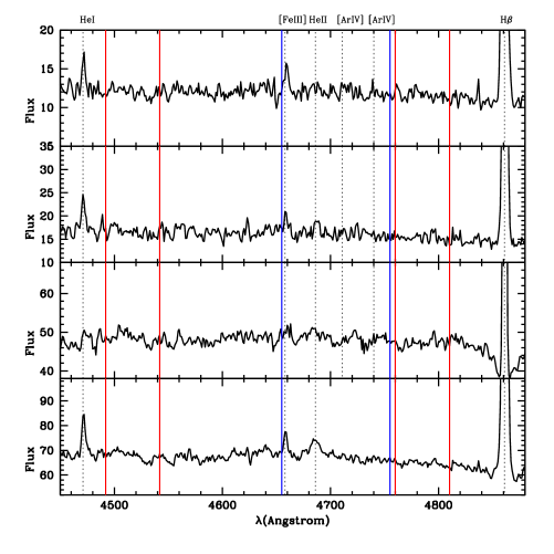
Figure 5: The top three panels show examples of three blue bump Wolf Rayet candidates with $S/N>10$ from the H$\alpha$ excess sample. The central bandpass is delineated by blue lines and the two continuum bandpasses by red lines. The bottom panel shows the stacked spectrum of all candidates of similar $S/N$ where a broadened HeII line at 4686 Å is clearly visible.

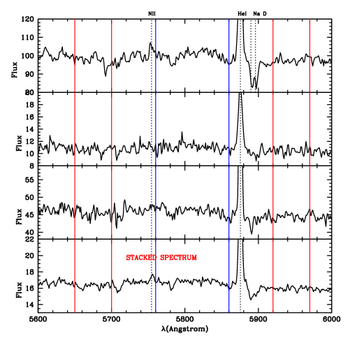
Figure 6: The top three panels show examples of red bump Wolf Rayet candidates with $S/N>10$ from the H$\alpha$ excess sample. The central bandpass is delineated by blue lines and the two continuum bandpasses by red lines. The bottom panel shows the stacked spectrum of all candidates of similar $S/N$.

In a few MaNGA galaxies with red Wolf Rayet features studied by Kauffmann (2021), a narrow CIV$\lambda$5808 emission line was clearly detected in the red bump window and the the strength of the feature increased strongly towards the central regions of the galaxy. The CIV$\lambda$5808 line was narrow indicating an O star rather than Wolf Rayet star origin. Nevertheless, an increase in emission from massive young stars combined with a flat or centrally rising 4000 Å break strength is difficult to reconcile with a universal IMF, so the study of the line emission in this wavelength interval is of potential interest in constraining the relative fractions of the very most massive stars that form in the very central regions of these galaxies.

These MaNGA galaxies were typically located at redshifts 0.02-0.05, whereas the galaxies in this sample are at median redshift $z=0.2$ where the 3 arcsec diameter SDSS fibres enclose stars out to a radius of 5 kpc, which is typically well within the disk. If the CIV$\lambda$5808 emission is mainly confined to the central stellar populations within galactic bulges, it is not surprising that it is considerably diluted in the spectra of more distant galaxies.

2.3 Radio-loud subset

We have cross-matched the H$\alpha$ excess and control samples with the source catalog from the Faint Images of the Radio Sky at Twenty-Centimeters (FIRST) survey carried out at the VLA (Condon et al. 1998), The SDSS and FIRST positions are required to be within 3 arc seconds of each other (see for example, Best et al 2005). We recover 208 VLA FIRST survey cross-matches in the H$\alpha$ excess sample, compared to 134 in the control sample, i.e. a 55% higher detection rate.

Table 2 provides the main derived quantities analyzed in this paper for the H$\alpha$ excess sample. A corresponding table for the control sample galaxies is also provided as part of the online supplementary material that accompanies this paper.

Table 2: Table of derived quantities for the H$\alpha$ excess sample. The columns are as follows: 1) SN_B(H$\alpha$), signal-to-noise of H$\alpha$ asymmetric flux detection on blue side, 2) F_B(H$\alpha$), fraction of total blue side H$\alpha$ flux in asymmetric component, 3) V80_B(H$\alpha$), wavelength enclosing 80% of the total blue side asymmetric flux, 4) SN_R(H$\alpha$), signal-to-noise of H$\alpha$ asymmetric flux detection on red side, 5) F_R(H$\alpha$), fraction of total red side H$\alpha$ flux in asymmetric component, 6) V80_R(H$\alpha$), wavelength enclosing 80% of the total red side asymmetric flux, 7) logarithm of radio power (Watts/Hz), 8) signal-to-noise of Wolf Wayet blue feature detection, 9) equivalent width of Wolf Rayet blue feature

SNB(H$\alpha$)	FB(H$\alpha$)	V80B(H$\alpha$)	SNR(H$\alpha$)	FR(H$\alpha$)	V80R(H$\alpha$)	log P (Watts/Hz)	SN WRB	EQW WRB
0.000	0.000	0.000	0.000	0.000	0.000	0.000	0.000	0.000
0.748	0.000	0.000	4.518	0.046	6576.753	0.000	0.000	0.000
0.000	0.000	0.000	0.000	0.000	0.000	0.000	0.000	0.000

3 Results for individual galaxies

In the section we compare the fraction of galaxies with H$\alpha$ line asymmetries, Wolf Rayet features and radio detections in the H$\alpha$ excess and control samples. We also study the correlations between these quantities with a variety of different host galaxy properties.

3.1 H$\alpha$ emission line profile asymmetries

We find that 126 out of 340 galaxies in the H$\alpha$ excess sample have detectable asymmetries, compared to 69 out of 340 galaxies in the control sample, i.e. the rate is 80% higher in the H$\alpha$ excess sample.

In Figure 7, we present the properties of the narrow H$\alpha$ line emission. The left panel shows the wavelength of the centroid of the single-Gaussian fit. This is strongly peaked at 6562.8 Å with only handful of galaxies showing centroid line shifts of greater than 0.5 Å. The right panel shows the distribution of the Gaussian width of the lines; the majority of galaxies have $\sigma$ in the range 100-150 km/s. The instrumental resolution of the SDSS spectrograph is 70 km/s, so these measurements correspond to true gas velocity dispersions in the range 70-130 km/s. These results show that narrow-line H$\alpha$ emission is detected in all the galaxies in the sample – there are no galaxies where the corrected single component line width is greater than 240 km/s. The fact that we are able to detect and quantify residual emission components is due to the fact that the lines are extremely strong and are detected with very high $S/N$.

Figure 7: The left panel shows the wavelength of the centroid of the single-Gaussian fit. The dotted line indicates a wavelength of 6562.8 ÅṪhe right panel shows the distribution of the Gaussian width $\sigma$ (uncorrected for instrumental resolution) of the lines.

In Figure 8, we plot 1)F(H$\alpha$), the fraction of the total H$\alpha$ flux in the offset line components and 2)V80, the velocity separation enclosing 80% of the asymmetric flux, as a function the stellar mass and the mean stellar age of the galaxies in the H$\alpha$ excess sample. If excess flux is detected on both the blue and the red side of the H$\alpha$ line centroid, we plot the maximum of the two measurements. Later on we will explore whether there are differences between the H$\alpha$ emission bluewards and redwards of the line centroid.

Figure 8: The top panels show V80, the velocity separation enclosing 80% of the asymmetric flux, as a function the stellar mass and the mean stellar age of the galaxies in the H$\alpha$ excess sample. The bottom panels show F(H$\alpha$), the fraction of the total H$\alpha$ flux in the offset line components as a function of the same. The Pearson correlation coefficient is given in the two bottom panels.

Figure 8 shows that F(H$\alpha$) varies between 0.05 and 0.25, with fairly strong dependence on stellar mass, but no dependence on mean stellar age. In contrast, in the sample of high redshift galaxies and AGN studied by Förster-Schreiber at al (2019), the flux in the broad components often exceeded the flux in the narrow component by a factor of two at the highest stellar masses and in the AGN. Our measurements of V80 appear to be divided into two well-separated classes – galaxies where the excess emission is offset by less than 200 km/s from the systemic velocity and those where the excess emission extends beyond 500 km/s. The latter class are almost always found in galaxies with stellar masses greater than $10^{10}M_{\odot}$ and the former class are found uniformly across the entire stellar mass range. V80 also does not depend on the mean stellar age of the galaxy. Figure 9 shows the same two quantities as a function of the Balmer decrement H$\alpha$/H$\beta$ and the extinction corrected H$\alpha$ equivalent width. F(H$\alpha$) shows a significant correlation with the Balmer decrement and a weaker dependence on EQW(H$\alpha$). There is a tendency for systems with large V80 to have higher Balmer decrements, but this is not as pronounced as the stellar mass dependence shown in Figure 8.

Figure 9: The top panels show V80, the velocity separation enclosing 80% of the asymmetric flux, as a function the Balmer decrement and the logarithm of the extinction corrected H$\alpha$ equivalent width of the galaxies in the H$\alpha$ excess sample. The bottom panels show F(H$\alpha$), the fraction of the total H$\alpha$ flux in the offset line components as a function of the same. The Pearson correlation coefficient is given in the two bottom panels.

Why is the distribution of the V80 parameter separated into two distinct peaks? In Figure 10, we have divided H$\alpha$ excess sample with detectable H$\alpha$ line asymmetries into three separate classes. In the figure red points show galaxies where the excess flux is on the red side of the H$\alpha$ line centrod, blue points show galaxies where it is on the blue side and green points show galaxies where excess emission is found on both sides of the line. We show the location of these three classes in a number of diagnostic plots. Blue side systems always have V80 less than 200 km/s. In red side systems, the excess emission usually extends to velocities of 500 km/s or greater. Red side systems also have higher Balmer decrement values than blue side systems, particularly for lower ionization ([OIII]/H$\beta$ ratio) systems Interestingly, the average F(H$\alpha$) values for blue and red side systems are the same ($\sim$ 0.1).

We also note that there appears to be a third, sparsely populated class of galaxies with V80$\sim$1000 km/s and where galaxies with both blue and red side components are found. These galaxies, shown as green points, have the highest [OIII]/H$\beta$ ratios and a significant fraction are found in the region of the BPT diagram occupied by AGN and composite galaxies.

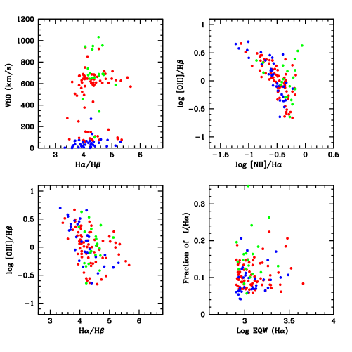
Figure 10: The top left panel shows V80, the velocity separation enclosing 80% of the asymmetric flux as a function the Balmer decrement. The top right panel shows the [OIII]/H$\beta$ versus [NII]/H$\alpha$ BPT diagram. The bottom left panel shows [OIII]/H$\beta$ versus the Balmer decrement. the bottom right panel shows the F(H$\alpha$) as a function of the logarithm of the extinction corrected H$\alpha$ equivalent width.

We note that Concas et al (2019) studied the incidence of neutral and ionized gas outflows in typical samples of galaxies in the local Universe and found that extended high-velocity H$\alpha$ emission was only found in AGN and not in the normal star-forming galaxy population. Förster-Schreiber et al (2019) studied H$\alpha$ line profile properties in a sample of typical galaxies at redshifts 0.6-2.7 and found that extended H$\alpha$ emission was found in both star-forming galaxies and AGN, but that there was a strong dichotomy in the velocity extent of the H$\alpha$ emission between star-forming galaxies and AGN. Here we have selected a subset of the most strongly star-forming galaxies (as traced by their H$\alpha$ emission) in the local Universe. The galaxies plotted in green in Figure 10 with the highest values of F(H$\alpha$) and V80 appear to be the closest analogues of the AGN studied by Concas et al (2019) and Förster-Schreiber et al (2019). AGN are only apparent in a very small minority of our H$\alpha$ excess sample, but insofar as they are found, they do seem to exhibit high velocity outflows of ionized gas.

It is then reasonable to speculate that the blue-shifted, low velocity H$\alpha$ components correspond to outflows generated by young stars and that broadened components appear on the blue side of the line, because the emission on the red side of the line is preferentially absorbed by dust. What then are the red-shifted, intermediate velocity (500-600 km/s) components? One possibility is that we are seeing inflowing rather than outflowing material that is triggering the formation of the very massive star population. Further study of well-resolved nearby systems using IFU data would be very useful to investigate these issues in more detail.

Finally, in Figure 11 we compare the relations between V80 and F(H$\alpha$) and stellar mass $M_{*}$ for galaxies with detected line asymmetries in the H$\alpha$ excess (red) and control sample (black). As we previously noted, there are many fewer such galaxies in the control sample. They appear to be shifted to somewhat higher stellar masses, but have similar distributions of V80 and F(H$\alpha$) at fixed $M_{*}$.

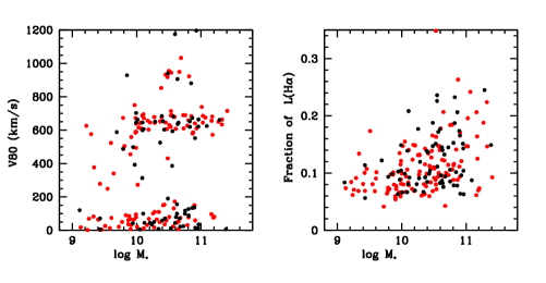
Figure 11: The relations between V80 and F(H$\alpha$) and stellar mass $M_{*}$ for galaxies with detected line asymmetries are plotted for galaxies in the H$\alpha$ excess (red) and control samples (black).

3.2 Wolf Rayet features

Our procedure for selecting candidate Wolf Rayet galaxies identified 62 blue bump and 69 red bump objects in the H$\alpha$ excess sample, and 54 blue bump and 52 red bump objects in the control sample. The distribution of $S/N$ values for the detections is shown in Figure 12. The average $S/N$ of the blue bump detections in the control sample is higher than in the H$\alpha$ excess sample. In section 4, we will explain the cause of this using stacked spectra. The $S/N$ values for the red bump detections in the H$\alpha$ excess sample is slightly higher than in the control sample, but the difference is quite small.

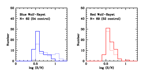
Figure 12: Left: The solid and dashed blue histograms show the $S/N$ distribution of the blue bump detections for the H$\alpha$ excess and control samples. Right: The solid and dashed red histograms show the $S/N$ distribution of the red bump detections for the H$\alpha$ excess and control samples.

In summary, the H$\alpha$ excess sample contains 15-20% more galaxies with suspected Wolf Rayet features compared to the control sample. This is considerably smaller than the factor 2-3 boost that was quoted in Kauffmann (2021). This likely indicates that Wolf Rayet signatures become more strongly diluted if the spectra include additional light from the outer galaxy. As we will show in the next section, physical information about the stellar populations of blue bump Wolf Rayet galaxies can still be extracted from the stacked spectra of galaxies at $z\sim 0.2$.

In the top panels of Figure 13, we plot mean stellar age as a function of stellar mass (left) and the Balmer decrement (right) for all galaxies from the H$\alpha$ excess sample (small black points), for blue bump Wolf Rayet candidates with $S/N>4$ (blue points) and for red bump Wolf Rayet candidates with $S/N>4$ (red points). In the bottom panels we plot the metallity indicator O3N2 as a function of the same two quantities. The O3N2 index depends on two (strong) emission line ratios and was first introduced and defined by Alloin et al. (1979) as O3N2=log([OIII]$\lambda$5007/H$\beta$-log([NII$\lambda$6583/H$\alpha$). Figure 13 shows that the blue and red bump Wolf Rayet candidates separate fairly strongly by stellar mass and metallicity, with the blue bump objects located mainly in galaxies with stellar masses less than $10^{10}M_{\odot}$ and the red bump objects distributed fairly uniformly across the whole mass range from $10^{9}-10^{11}M_{\odot}$.

We will show in the next section that our blue bump detections are confirmed as true Wolf Rayet galaxies in stacked spectra by the detection of a clearly broadened HeII$\lambda$4686 line, but the same is not true for our red bump detections. We thus caution the reader against reading too much into these findings at this stage. We also note that the Wolf Rayet candidates have somewhat younger mean stellar age estimates at fixed stellar mass than the underlying sample, but the age shift is rather weak and is only apparent for more massive galaxies. There is no offset in mean stellar age at fixed Balmer decrement H$\alpha$/H$\beta$. The weak shifts in mean stellar age may indicate that the youngest stars are only a very small fraction of the total stellar mass probed by the fibre. Alternatively, the light from many of the youngest stars may be heavily attenuated by dust. We will discuss this in more detail in the final section of the paper.

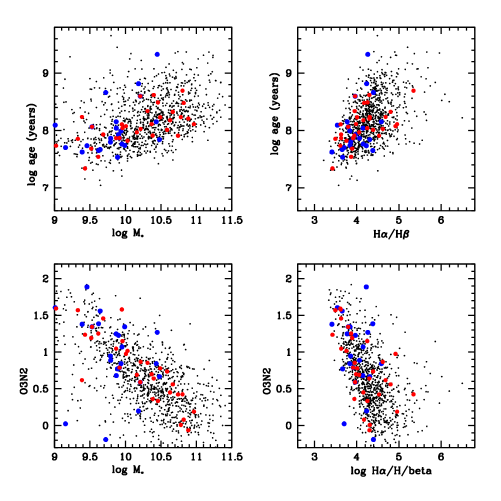
Figure 13: Top panels: mean stellar age is plotted as a function of stellar mass (left) and the Balmer decrement (right) for all galaxies from the H$\alpha$ excess sample (small black points), for blue bump Wolf Rayet candidates with $S/N>4$ (blue points) and for red bump Wolf Rayet candidates with $S/N>4$ (red points). Bottom panels: the metallity indicator O3N2 is plotted as a function of the same two quantities.

3.3 Radio detections

We recover 208 VLA FIRST survey cross-matches in the H$\alpha$ excess sample, compared to 134 in the control sample, i.e. a 55% higher detection rate. Figure 14 shows histograms of the stellar masses and mean stellar ages of the galaxies in the radio-loud subsamples compared to their parent samples. In the left panels, we compare the radio-loud subsample extracted from the H$\alpha$ excess sample (solid histograms) with the parent H$\alpha$ excess sample (dotted histograms). The radio-loud samples are shifted to higher stellar masses and older mean stellar ages. In the middle panels, we compare the radio-loud subsample extracted from the control samples and find a similar shift to larger stellar masses and older ages. In the right panels, we compare the radio loud subsamples from the H$\alpha$ excess and control samples with each other, finding a shift towards younger stellar populations for radio-loud galaxies from the H$\alpha$ excess sample in comparison to the radio-loud control galaxies. These controlled comparisons yield evidence that the higher level of radio activity amongst the H$\alpha$ excess galaxies may be tied to the presence of young stars.

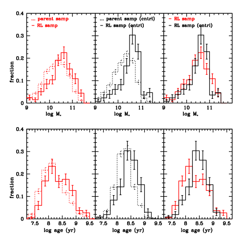
Figure 14: Histograms of the stellar masses and mean stellar ages of the galaxies in the radio-loud subsamples compared to their parent samples. Left panels: the radio-loud subsample extracted from the H$\alpha$ excess sample (solid histograms) and the parent H$\alpha$ excess sample (dotted histograms). Middle panels: the radio-loud subsample extracted from the control samples (solid) and the full control sample (dotted). Right panels: the radio loud subsamples from the H$\alpha$ excess (red solid) and control samples (black solid). Error bars on the histograms are computed via a standard bootstrap resampling technique.

Figure 15 explores relations between the radio luminosities of the galaxies with VLA FIRST detections in the H$\alpha$ excess sample (red points) and in the control sample (black points) with different host galaxy properties. The top left panel shows that there is a strong correlation between radio power P and stellar mass in both samples, with the control sample galaxies shifted to higher stellar masses as indicated in Figure 14. In the next three panels, we scale out the stellar mass dependence and plot the ratio of radio power to stellar mass as a function of H$\alpha$ equivalent width, Balmer decrement and mean stellar age. The quantity $\log P/M_{*}$ only shows a fairly strong residual dependence with mean stellar age. $P/M_{*}$ is on average a factor of 10 larger for galaxies with mean stellar ages of a few$\times 10^{7}$ years than it is for galaxies with stellar ages of $\sim 10^{9}$ years. This again provides evidence that the radio emission is linked to the presence of young stars.

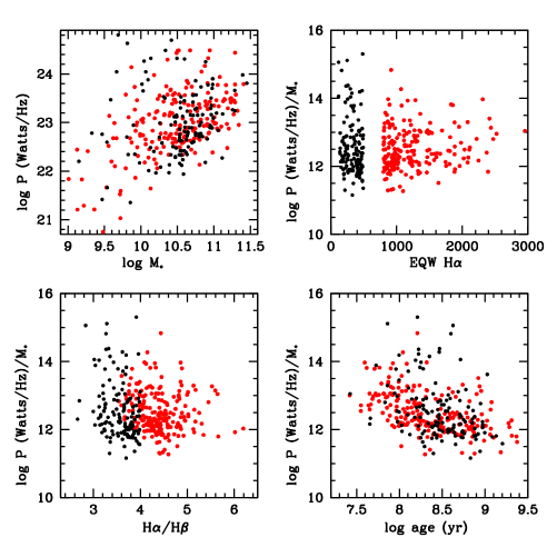
Figure 15: Top left: correlation between radio power P and stellar mass. VLA FIRST detections in the H$\alpha$ excess sample are plotted as red points and in the control sample as black points. Top right: the ratio of radio power to stellar mass ( $\log P/M_{*}$) as a function of H$\alpha$ equivalent width. Bottom left: $\log P/M_{*}$ as a function of Balmer decrement. Bottom right: $\log P/M_{*}$ as function of mean stellar age.

FIRST cut-out images of the most radio-luminous galaxies in the sample to see if there is any evidence for AGN-powered jets in these galaxies and we find that the majority are unresolved point sources. There are a handful of galaxies where more than one point source is detected and these are usually merging/interacting systems. The brightest source in the sample with $\log(P/{\rm WattsHz}^{-1})>25$ does exhibit a classical jet-lobe morphology. Since it is the only one in the sample and the most extreme object, we remove it when carrying out the spectral stacking analysis described in the next section.

4 A search for additional physical information using stacked spectra

We now utilize stacked spectra as a way of gaining further insight into the main physical processes that could be at work in the H$\alpha$ excess sample. As outlined in section 1, it is of particular interest to investigate whether galaxies with evidence for unusual populations of young, massive stars may also be sites for the formation of intermediate mass black holes, or whether efficient accretion onto existing black holes may be occuring in such systems.

We have shown that the majority of galaxies fall well within the star-forming locus in the canonical [OIII]/H$\beta$ versus [NII]/H$\alpha$ BPT diagram, so any AGN contribution to the [OIII] line is heavily swamped by emission from the HII regions in these galaxies. Higher ionization lines, such as [NeV]$\lambda$3345 and [NeV]$\lambda$3425 provide possible AGN diagnostics where ionization from young stars is likely to be much less important. It has been shown that highly obscured, Compton thick (column density $N_{H}>10^{24}-10^{25}$ sm^-2) AGN hosted in massive star-forming galaxies sometimes show strong [NeV] emission (Gilli et al 2010; Lanzuisi et al 2018). We note that the detection of [NeV] is not, in and of itself, an existence proof of an accreting black hole. Izotov, Thuan & Privon (2012) have identified [NeV] emission lines in a number of blue compact dwarf galaxies and favour an explanation where the emission arises from fast, radiative shocks associated with the starburst itself.

In this analysis, we have split the full H$\alpha$ excess sample into sub-samples according to properties such as 1) radio luminosity, 2) presence or absence of H$\alpha$ line asymmetries extending to high velocities, and 3) presence or absence of Wolf Rayet signatures. We create stacked spectra for each of these subsamples and investigate key spectral regions for systematic trends. For example, if the strength of the [NeV] line were found to scale with the radio luminosity of the system, this might provide evidence that shocks induced by a relativistically expanding jet were responsible for both the radio emission and the excitation of the hard ionizing radiation.

4.1 Spectra stacked by radio luminosity

Figure 16 shows spectra stacked according their radio properties – we plot spectra for H$\alpha$ excess sample galaxies with no radio detection in black, for all galaxies with a VLA FIRST radio detection in green, for galaxies with $22.5<\log(P/{\rm WattsHz}^{-1})<23.5$ in blue, and for galaxies with $23.5<\log P/{\rm WattsHz}^{-1})<24.5$ in red. The top right panel shows the spectral range covering the [NeV]$\lambda$3345 and [NeV]$\lambda$3425 emission lines. There is no detectable [NeV] emission for the sample without radio detections. Only for the two highest radio luminosity bins are there clear detections of [NeV]$\lambda$3425. The line is broadened in comparsion to the [OIII] lines shown in the bottom left panel of the figure. The [NeV]$\lambda$3425 line exhibits a hint of a double-peaked profile, which has been proposed as a signature of jet-interstellar medium interactions in galaxies (e.g. Rubinur & Kharb 2019, Kharb et al 2021).

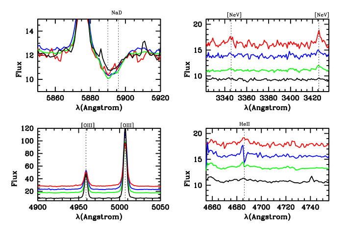
Figure 16: Spectra stacked according their radio properties. The stacked spectrum for H$\alpha$ excess sample galaxies with no radio detection is plotted in black, for all galaxies with a VLA FIRST radio detection in green, for galaxies with $22.5<\log P/{\rm WattsHz}^{-1})<23.5$ in blue, and for galaxies with $23.5<\log(P/{\rm WattsHz}^{-1})<24.5$ in red. The top left panel shows the region of the spectrum around the Na I $\lambda\lambda$5890, 5896 (Na D) aborption line doublet (The position of the doublet is marked using dotted lines.) The top right panel shows the spectral range covering the [NeV]$\lambda$3345 and [NeV]$\lambda$3425 emission lines. The bottom left panel shows the spectral range covering the [OIII]$\lambda$4959 and [OIII]$\lambda$5007 emission lines. The bottom right panel shows the spectral region around HeII$\lambda$4686.

The bottom right panel of Figure 16 shows the spectral region around HeII$\lambda$4686, another high ionization emission line. The stacked spectrum of the strongest radio sources again shows a broadened, double-peaked line. Interestingly, HeII$\lambda$4686 in the stacked spectrum of the intermediate luminosity sources with $22.5<\log(P/{\rm WattsHz}^{-1})<23.5$ exhibits a clear inverse P-Cygni profile, with one component in emission bluewards of the expected line centre, and another component in absorption on the red ride of the line. Inverse P-Cygni profiles are believed to be a diagnostic of infalling gas. They are a characteristic feature of molecular line observations of protostars. The same line profile shape is still visible for the stack of the full sample of radio-loud galaxies plotted in green, but the emission and absorption components are much weaker. The stacked spectrum of galaxies without radio detections does not exhibit HeII emission.

The two right panels of Figure 16 demonstrate that very high ionization emission lines are strongest for the most luminous radio sources in the H$\alpha$ excess sample. Comparison of the [OIII]$\lambda$4959 and [OIII]$\lambda$5007 emission lines for stacked spectra with different radio luminosities show that the opposite is true. These lines get progressively weaker at high radio luminosities. The [OIII] lines are also very regular with no clear broadened components or asymmetries. This suggests that these lines trace very different gas components. Unfortunately there is no information from single fibre spectra about the spatial scale of the emission, but one might hypothesize from the regularity of the line profiles that the [OIII]-emitting gas is in virial equilibrium with the stars in the galaxy, whereas the higher ionization lines come from more localized sources.

Why are lines traced by the global galaxy gas component weaker in the radio-loud systems? The top left panel of Figure 16 shows the region of the spectrum around the Na I $\lambda\lambda$5890, 5896 (Na D) sborption line doublet. This absorption line has been used as a probe of the kinematics of cool, neutral gas in galaxies (Chen et al 2010; Concas et al 2018). In normal star-forming galaxies, the lines can be separated into two components: a quiescent disk-like component at the galaxy systemic velocity and a blue-shifted outflow component, which becomes stronger in galaxies with higher star formation surface densities and dust content. The galaxies in the H$\alpha$ excess sample are found to have rather irregular morphologies on average, so it is perhaps not surprising that the NaD doublets in the stacked spectra appear more blended that in previous studies of normal star-forming galaxies. Nevertheless. Figure 16 shows a clear bluewards shift of the absorption line profile for the radio-loud galaxies compared to the galaxies with no radio detections. This is an indication of more neutral outflowing gas in the radio-loud sample. However, there is no clear correlation of line shift with radio luminosity – all the radio-loud subsamples have approximately the same NaD absorption line profiles. This suggests that the main energy source for the outflows is not the same as for the radio emission, and is most likely star formation.

4.2 Spectra stacked according to the presence of high-velocity H$\alpha$ line components

In this section, we examine stacked spectra of two subsets of the H$\alpha$ excess sample: 1) those with no detectable H$\alpha$ line profile asymmetries, 2)those with “fast” outflows with $V80>500$ km/s. In Figure 17, the stacked spectrum of subsample (1) is plotted in blue and that of subsample (2) in red over the same wavelength ranges as in Figure 16.

Figure 17 shows that high ionization lines are weak in both spectral stacks and show no differences according to whether or not high-velocity H$\alpha$ line components are detected. The [OIII] line is somewhat weaker in the stack with high velocity H$\alpha$ components and the NaD absorption feature shows a stronger blueshift. These trends are consistent with the hypothesis that the high-velocity H$\alpha$ components trace outflowing gas from the galaxy.

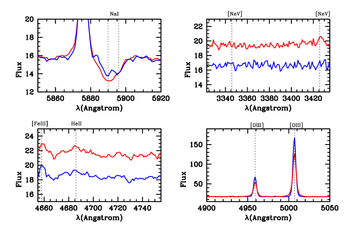
Figure 17: As in Figure 16, but for spectra stacked according to whether or not aysymmetric H$\alpha$ line components with $V80>500$ km/s are found. The stacked spectrum for H$\alpha$ excess sample galaxies with high velocity H$\alpha$ components is plotted in red, and for H$\alpha$ excess sample galaxies with no detectable line asymmetries in blue.

4.3 Spectra stacked according to the blue and red bump detections

Figure 18 compares the stacked spectra of galaxies from the H$\alpha$ excess and control samples with blue bump detections with $S/N>4$. The procedures for measuring the blue and red bumps have been outlined in Section 2.2. The HeII$\lambda 4686$ emission line is strong in both the H$\alpha$ excess and the control sample stacked spectra. In the H$\alpha$ excess stack, HeII$\lambda$ 4686 line is broader than the higher ionization [FeIII]$\lambda$4658 line (FWHM$\sim$ 15 Åfor HeII compared to 3 Å for [FeIII]). This is suggestive of a late WN population (Crowther & Walborn 2011). In the control sample stack, the HeII $\lambda$4686 line is similar in width to H$\beta$, suggesting a nebular origin. HeI is stronger in the H$\alpha$ excess stack and the high ionization [ArIV] lines are stronger in the control sample stack.

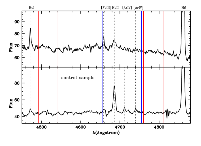
Figure 18: Stacked spectra of galaxies from the H$\alpha$ excess (top) and control samples (bottom) with blue bump detections with $S/N>4$ over the spectral region covering the blue bump. The central bandpass is delineated by blue lines and the two continuum bandpasses by red lines.

Figure 19 shows the same comparison for galaxies with red bump detections in the two samples. The stack from the H$\alpha$ excess sample is characterized by strong interstellar absorption features. The strongest of these is the NaD doublet marked in the figure. In many starburst galaxies, the only narrow emission line that is usually detected in red bump identifications is [NII]$\lambda$5755 (see Figure 2 of López-Sánchez & Esteban (2018)). This line is clearly visible in our H$\alpha$ excess stack, but not in the control sample stack.

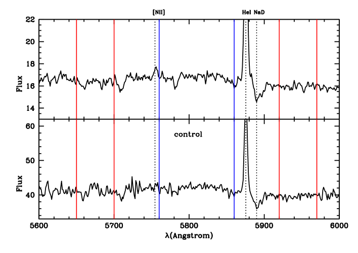
Figure 19: Stacked spectra of galaxies from the H$\alpha$ excess (top) and control samples (bottom) with red bump detections with $S/N>4$ over the spectral region covering the red bump. The central bandpass is delineated by blue lines and the two continuum bandpasses by red lines.

In Figure 20, we examine the spectral region covering [NeV]$\lambda$3345 and [NeV]$\lambda$3425 (left panels) and [NeIII]$\lambda$3869 and [NeIII]$\lambda$3967 (right panels) for the 4 sets of stacked spectra shown in Figures 18 and 19. The [NeV] lines are not detected in either of the H$\alpha$ excess stacks. Strong [NeV] lines are detected only in the control sample stack. The lines are similar in width and shape to the HeII$\lambda$ 4686 line shown in the bottom panel of Figure 18, so it is likely that the source of ionization is the same for both. Tha ratio HeII$\lambda 4686$/H$\beta$ in this stack is 0.34, which would classify them as AGN in the HeII emission line diagnostic diagram introduced by Shirazi & Brinchmann (2012). These authors showed that HeII-strong AGN were found mainly in star-forming galaxies on the blue cloud and on the main sequence where ionization from star formation is most likely to mask AGN emission in the BPT lines. In follow-up work, Bär et al (2017) cross-matched a sample of 234 He II-only AGN candidates with the Chandra Source Catalog (Evans et al. 2010). Among 12 objects with X-ray detections, five objects were confirmed as AGN based on their X-ray luminosity and power-law nature; of the remaining seven objects, six objects had X-ray luminosity upper limits consistent with being AGN.

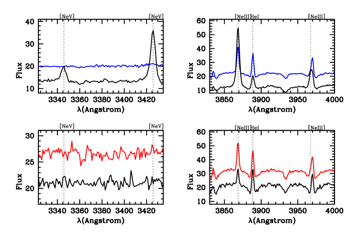
Figure 20: The spectral region covering [NeV]$\lambda$3345 and [NeV]$\lambda$3425 (left panels) and [NeIII]$\lambda$3869 and [NeIII]$\lambda$3967 (right panels) for the 4 sets of stacked spectra shown in Figures 18 and 19. The blue bump and control stacks are shown in the top panels, plotted in blue and black. The red bump and control stacks are shown in the top panels, plotted in red and black.

We have postulated that our control sample galaxies represent a later stage of a stong star-forming episode compared to the H$\alpha$ excess galaxies. In the H$\alpha$ excess sample, the HeII$\lambda 4686$ emission is found to be produced by Wolf Rayet stars and in the control sample, the HeII$\lambda 4686$ is likely produced by an accreting black hole. It is thus very tempting to speculate that there is an evolutionary sequence from an environment that is very rich in massive stars to an environment that contains one or more black holes in formation.

5 Summary of findings and future perspectives

We have selected two samples from the SDSS main galaxy sample on the basis of their extinction-corrected H$\alpha$ equivalent widths. The first sample is selected to have EQW(H$\alpha$/Å)$>800$ and is called the H$\alpha$ excess sample, because EQW(H$\alpha$) is too high to be explained by ionization by a young stellar population with a normal initial mass function (IMF). We create a control sample where galaxies are matched to each H$\alpha$ excess galaxy in stellar mass, redshift and 4000 Å break strength, but where the H$\alpha$ EQW is in the range 80-300 Å, typical of strongly star-forming galaxies with a normal IMF.

We carry out a systematic comparison of the two samples, with the following main findings:

• The H$\alpha$ excess galaxies have median stellar mass of $2\times 10^{10}M_{\odot}$. They have younger mean stellar ages and more dust than the control sample galaxies. Almost all galaxies in both samples lie within the star-forming locus in the [OIII]/H$\beta$ versus [NII]/H$\alpha$ BPT diagram.

• H$\alpha$ excess galaxies are twice as likely to exhibit H$\alpha$ line profile asymmetries compared to control sample galaxies.

• The fraction of the total H$\alpha$ flux in the asymmetric components ranges between 0.05 and 0.25 and is larger for more massive galaxies and galaxies with higher dust extinction.

• Two distinct types of H$\alpha$ line profile asymmetries are identified: a) Blue-shifted H$\alpha$ components that extend over velocity separations of less than 200 km/s from the systemic redshift b) Red-shifted H$\alpha$ components that extend to velocities of 500 km/s or greater. The galaxies with the highest velocity H$\alpha$ components ($>1000$ km/s) have BPT line ratios indicative of AGN ionization.

• H$\alpha$ excess galaxies are 1.55 times as likely to have radio detections in the VLA FIRST catalogue compared to control sample galaxies. In the H$\alpha$ excess sample, radio luminosity per unit stellar mass is a factor of 10 larger for galaxies with stellar ages $\sim 10^{7.5}$ yr compared to galaxies with stellr ages $\sim 10^{9}$ yr.

• The stacked spectra of H$\alpha$ excess galaxies with the highest radio luminosities exhibit high ionization [NeV]$\lambda$3345, [NeV]$\lambda$3425 and HeII$\lambda$4686 emission. The line shapes of the high ionization lines are complex: they are sometimes broadened and they sometimes exhibit inverse P-cygni profiles indicative of gas inflow.

• We search for emission from very young Wolf Rayet stars by looking for excess emission over the wavelength ranges 4665-4755 Å and 5760-5860 Å. Similar numbers of candidates are found for both the H$\alpha$ excess and control samples. The stacked spectrum of WR candidates from the H$\alpha$ excess sample reveals a broadened HeII$\lambda$4686 line characteristic of WN star emission and no high-ionization [NeV] lines. In contrast, the stacked spectrum of WR candidates from the control sample reveals a narrow HeII$\lambda$4686 line and strong [NeV]$\lambda$3345 and [NeV]$\lambda$3425 emission characteristic of AGN.

In summary, we have utilized a diverse range of indicators to probe the H$\alpha$ excess sample for hidden populations of accreting black holes. We find a strong correlation between radio luminosity per unit stellar mass and mean stellar age such that log P/$M_{*}$ increases for the systems with the youngest stellar populations. We also find that the [NeV] emission line strength correlates with radio luminosity in the H$\alpha$ excess sample. [NeV] emission is not present in the very youngest radio-quiet H$\alpha$ excess galaxies with detectable Wolf-Rayet features. Although correlations of the kind presented in this paper suggest a causal connection between star formation, black hole formation/accretion and the generation of radio jets, a campaign to spatially map the emission from representative samples of such objects is required to establish a true picture of what is happening within these very dense star-forming regions.

Our study has also revealed the promise of spectral stacking as a way of pulling out the weaker line emission associated with short-lived, high mass stars. Synthetic spectra of the most massive stars calculated from model atmospheres which account for non-LTE, spherical expansion and and metal line blanketing (Hamman & Gräfener 2004) can be incorporated into stellar population synthesis codes. The HR-pyPopStar model (Millán-Irgoyen et al 2021) provides a complete set of high resolution spectral energy distributions of single stellar populations. The model incorporates high wavelength-resolution theoretical atmosphere libraries for main sequence, post-AGB/planetary nebulae and Wolf-Rayet stars and is an update of the models presented in Mollá, García-Vargas & Bressan (2009). Figure 21 shows HR-pyPopStar SSPs plotted over the wavelength range that includes the main blue Wolf Rayet features. The spectra have been smoothed to 2 Åresolution to be more directly comparable to our SDSS spectra. Results are shown for solar metallicity models and a Chabrier (2003) IMF at six different times from $10^{6}-10^{7}$ years. The development of a broad feature around the HeII $\lambda$4686 line commences at an age of 3$\times 10^{6}$ years and is over by an age of 5$\times 10^{6}$, i.e. it is a very short phase in the evolution of a simple stellar population. The [FeIII]$\lambda$4658 line is present in emission until a time of 3$\times 10^{6}$ yr. The blue spectrum plotted in the left middle panel of Figure 21 shows the HR-pyPopStar SSP for a 0.4 solar model for comparison. [FeIII]$\lambda$4658 emission is not present at this lower metallicity. In Figure 22, we overplot HR-pyPopStar solar metallicity SSPs at time $\log(t/{\rm yr})=6.48$ (red solid lines) and $\log(t/{\rm yr})=6.54$ (red dotted lines) on the stacked spectrum of H$\alpha$ excess sample galaxies with blue bump detections (black solid lines). Both SSPs fit the [FeIII]$\lambda$4658 line. The width of the broad HeII $\lambda$4686 is in good agreement with the data, but the amplitude of the feature is too low to match the observations.

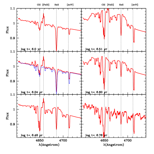
Figure 21: HR-pyPopStar SSPs plotted over the wavelength range that includes the main blue Wolf Rayet features. The spectra have been smoothed to 2 Åresolution to be more directly comparable to our SDSS spectra. Results are shown for solar metallicity models and a Chabrier (2003) IMF at six different times from $10^{6}-10^{7}$ years. The blue spectrum plotted in the left middle panel of Figure 21 shows the HR-pyPopStar SSP for a 0.4 solar model for comparison.

Past work has also found that SSP models underpredict blue optical Wolf Rayet bumps. Sidoli et al (2006) analyzed the spectrum of the giant HII region Tol89 in NGC5398, inferring the O star content from the stellar continuum and using STARBURST99 models to predict optical WR features using the grids from Smith et al. (2002). They found that the models underpredict the WR features and attributed this failure to the neglect of rotational mixing in evolutionary models. Evolutionary mixing increases the lifetimes of WR phases as a result of the increased duration of the H-rich phase, and lowers the initial mass limit for the formation of WR stars. This compromises the use of the WR features as diagnostics of other physical parameters such as stellar IMF or recent star formation history.

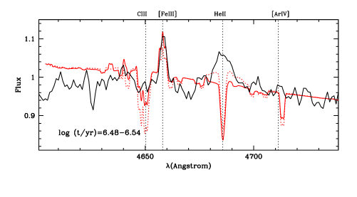
Figure 22: HR-pyPopStar solar metallicity SSPs at times $\log(t/{\rm yr})=6.48$ (red solid lines) and $\log(t/{\rm yr})=6.54$ (red dotted lines) are overplotted on the stacked spectrum from the H$\alpha$ excess sample with blue bump detections (black solid lines).

It is possible that by constructing grids of stacked empirical spectra from large galaxy samples drawn from IFU surveys such as MaNGA, and by studying how Wolf Rayet and continuum features scale with each other in a variety of galactic environments, insights may be obtained that serve to better constrain both stellar models and the possibly changing nature of young stellar populations in dense stellar environments. This will be the subject of future work.

Finally we note that many of the galaxies in the H$\alpha$ excess sample are quite highly reddened. This can be seen very clearly in Figure 22 from the negative offset in the observed continuum compared to the model continuum on the blue side of the wavelength window. Correcting for the effect of dust on spectral lines requires a model for the spatial distribution of the dust in HII regions. Simple models, e.g. Charlot & Fall (2000), may break down in very extreme galactic environments and follow-up near-infrared observations (e.g. Crowther et al 2006, Rosslowe & Crowther 2018) can serve to better constrain the true content of Wolf-Rayet stars in galaxies.

Acknowledgments
GK thanks Selma de Mink for helpful discussions related to this work.

Data Availability
The data underlying this article are available in the article and in its online supplementary material.

References

- Aird et al. (2012) Aird J., Coil A. L., Moustakas J., Blanton M. R., Burles S. M., Cool R. J., Eisenstein D. J., et al., 2012, ApJ, 746, 90. doi:10.1088/0004-637X/746/1/90
- Alloin et al. (1979) Alloin D., Collin-Souffrin S., Joly M., Vigroux L., 1979, A&A, 78, 200
- Bär et al. (2017) Bär R. E., Weigel A. K., Sartori L. F., Oh K., Koss M., Schawinski K., 2017, MNRAS, 466, 2879. doi:10.1093/mnras/stw3283
- Baldwin, Phillips & Terlevich (1981) Baldwin J. A., Phillips M. M., Terlevich R., 1981, PASP, 93, 5
- Balogh, et al. (1999) Balogh M. L., Morris S. L., Yee H. K. C., Carlberg R. G., Ellingson E., 1999, ApJ, 527, 54
- Baldassare et al. (2015) Baldassare V. F., Reines A. E., Gallo E., Greene J. E., 2015, ApJL, 809, L14. doi:10.1088/2041-8205/809/1/L14
- Begelman, Volonteri, & Rees (2006) Begelman M. C., Volonteri M., Rees M. J., 2006, MNRAS, 370, 289. doi:10.1111/j.1365-2966.2006.10467.x
- Best et al. (2005) Best P. N., Kauffmann G., Heckman T. M., Ivezić Ž., 2005, MNRAS, 362, 9. doi:10.1111/j.1365-2966.2005.09283.x
- Brinchmann, Kunth & Durret (2008) Brinchmann J., Kunth D., Durret F., 2008, A&A, 485, 657
- Bromm & Loeb (2003) Bromm V., Loeb A., 2003, ApJ, 596, 34. doi:10.1086/377529
- Bruzual & Charlot (2003) Bruzual G., Charlot S., 2003, MNRAS, 344, 1000. doi:10.1046/j.1365-8711.2003.06897.x
- Bundy et al. (2015) Bundy K., Bershady M. A., Law D. R., Yan R., Drory N., MacDonald N., Wake D. A., et al., 2015, ApJ, 798, 7. doi:10.1088/0004-637X/798/1/7
- Calzetti (2001) Calzetti D., 2001, PASP, 113, 1449. doi:10.1086/324269
- Cappellari & Emsellem (2004) Cappellari M., Emsellem E., 2004, PASP, 116, 138. doi:10.1086/381875
- Chabrier (2003) Chabrier G., 2003, PASP, 115, 763. doi:10.1086/376392
- Charlot & Fall (2000) Charlot S., Fall S. M., 2000, ApJ, 539, 718. doi:10.1086/309250
- Chen et al. (2012) Chen Y.-M., Kauffmann G., Tremonti C. A., White S., Heckman T. M., Kovač K., Bundy K., et al., 2012, MNRAS, 421, 314. doi:10.1111/j.1365-2966.2011.20306.x
- Comparat et al. (2017) Comparat J., Maraston C., Goddard D., Gonzalez-Perez V., Lian J., Meneses-Goytia S., Thomas D., et al., 2017, arXiv, arXiv:1711.06575
- Concas et al. (2019) Concas A., Popesso P., Brusa M., Mainieri V., Thomas D., 2019, A&A, 622, A188. doi:10.1051/0004-6361/201732152
- Condon et al. (1998) Condon J. J., Cotton W. D., Greisen E. W., Yin Q. F., Perley R. A., Taylor G. B., Broderick J. J., 1998, AJ, 115, 1693. doi:10.1086/300337
- Crowther et al. (2006) Crowther P. A., Hadfield L. J., Clark J. S., Negueruela I., Vacca W. D., 2006, MNRAS, 372, 1407. doi:10.1111/j.1365-2966.2006.10952.x
- Crowther & Walborn (2011) Crowther P. A., Walborn N. R., 2011, MNRAS, 416, 1311. doi:10.1111/j.1365-2966.2011.19129.x
- Dabringhausen, Kroupa, & Baumgardt (2009) Dabringhausen J., Kroupa P., Baumgardt H., 2009, MNRAS, 394, 1529. doi:10.1111/j.1365-2966.2009.14425.x
- Devecchi & Volonteri (2009) Devecchi B., Volonteri M., 2009, ApJ, 694, 302. doi:10.1088/0004-637X/694/1/302
- Evans et al. (2010) Evans I. N., Primini F. A., Glotfelty K. J., Anderson C. S., Bonaventura N. R., Chen J. C., Davis J. E., et al., 2010, ApJS, 189, 37. doi:10.1088/0067-0049/189/1/37
- Fan et al. (2003) Fan X., Strauss M. A., Schneider D. P., Becker R. H., White R. L., Haiman Z., Gregg M., et al., 2003, AJ, 125, 1649. doi:10.1086/368246
- Farrell et al. (2012) Farrell S. A., Servillat M., Pforr J., Maccarone T. J., Knigge C., Godet O., Maraston C., et al., 2012, ApJL, 747, L13. doi:10.1088/2041-8205/747/1/L13
- Förster Schreiber, et al. (2018) Förster Schreiber N. M., et al., 2018, ApJS, 238, 21
- Gilli et al. (2010) Gilli R., Vignali C., Mignoli M., Iwasawa K., Comastri A., Zamorani G., 2010, A&A, 519, A92. doi:10.1051/0004-6361/201014039
- Haghi et al. (2017) Haghi H., Khalaj P., Hasani Zonoozi A., Kroupa P., 2017, ApJ, 839, 60. doi:10.3847/1538-4357/aa6719
- Hamann & Gräfener (2003) Hamann W.-R., Gräfener G., 2003, A&A, 410, 993. doi:10.1051/0004-6361:20031308
- Heckman & Lehnert (2000) Heckman T. M., Lehnert M. D., 2000, ApJ, 537, 690. doi:10.1086/309086
- Hosek et al. (2019) Hosek M. W., Lu J. R., Anderson J., Najarro F., Ghez A. M., Morris M. R., Clarkson W. I., et al., 2019, ApJ, 870, 44. doi:10.3847/1538-4357/aaef90
- Izotov, Thuan, & Privon (2012) Izotov Y. I., Thuan T. X., Privon G., 2012, MNRAS, 427, 1229. doi:10.1111/j.1365-2966.2012.22051.x
- Kauffmann et al. (2003a) Kauffmann G., Heckman T. M., White S. D. M., Charlot S., Tremonti C., Peng E. W., Seibert M., et al., 2003, MNRAS, 341, 54. doi:10.1046/j.1365-8711.2003.06292.x
- Kauffmann, et al. (2003b) Kauffmann G., et al., 2003, MNRAS, 346, 1055
- Kauffmann (2021) Kauffmann G., 2021, MNRAS, 506, 727. doi:10.1093/mnras/stab1750
- Kauffmann & Heckman (2009) Kauffmann G., Heckman T. M., 2009, MNRAS, 397, 135. doi:10.1111/j.1365-2966.2009.14960.x
- Kharb et al. (2021) Kharb P., Subramanian S., Das M., Vaddi S., Paragi Z., 2021, ApJ, 919, 108. doi:10.3847/1538-4357/ac0c82
- Kroupa (2001) Kroupa P., 2001, MNRAS, 322, 231
- Lanzuisi et al. (2018) Lanzuisi G., Civano F., Marchesi S., Comastri A., Brusa M., Gilli R., Vignali C., et al., 2018, MNRAS, 480, 2578. doi:10.1093/mnras/sty2025
- Lodato & Natarajan (2006) Lodato G., Natarajan P., 2006, MNRAS, 371, 1813. doi:10.1111/j.1365-2966.2006.10801.x
- Loeb & Rasio (1994) Loeb A., Rasio F. A., 1994, ApJ, 432, 52. doi:10.1086/174548
- López-Sánchez & Esteban (2010) López-Sánchez Á. R., Esteban C., 2010, A&A, 516, A104. doi:10.1051/0004-6361/200913434
- Lu et al. (2013) Lu J. R., Do T., Ghez A. M., Morris M. R., Yelda S., Matthews K., 2013, ApJ, 764, 155. doi:10.1088/0004-637X/764/2/155
- Maraston et al. (2009) Maraston C., Nieves Colmenárez L., Bender R., Thomas D., 2009, A&A, 493, 425. doi:10.1051/0004-6361:20066907
- Maraston & Strömbäck (2011) Maraston C., Strömbäck G., 2011, MNRAS, 418, 2785. doi:10.1111/j.1365-2966.2011.19738.x
- Mezcua (2017) Mezcua M., 2017, IJMPD, 26, 1730021. doi:10.1142/S021827181730021X
- Millán-Irigoyen et al. (2021) Millán-Irigoyen I., Mollá M., Cerviño M., Ascasibar Y., García-Vargas M. L., Coelho P. R. T., 2021, MNRAS, 506, 4781. doi:10.1093/mnras/stab1969
- Mollá, García-Vargas, & Bressan (2009) Mollá M., García-Vargas M. L., Bressan A., 2009, MNRAS, 398, 451. doi:10.1111/j.1365-2966.2009.15160.x
- Natarajan (2021) Natarajan, P.: 2021, Monthly Notices of the Royal Astronomical Society 501, 1413. doi:10.1093/mnras/staa3724.
- Portegies Zwart, Dewi, & Maccarone (2004) Portegies Zwart S. F., Dewi J., Maccarone T., 2004, MNRAS, 355, 413. doi:10.1111/j.1365-2966.2004.08327.x
- Reines et al. (2011) Reines A. E., Sivakoff G. R., Johnson K. E., Brogan C. L., 2011, Natur, 470, 66. doi:10.1038/nature09724
- Reines & Deller (2012) Reines A. E., Deller A. T., 2012, ApJL, 750, L24. doi:10.1088/2041-8205/750/1/L24
- Reines, Greene, & Geha (2013) Reines A. E., Greene J. E., Geha M., 2013, ApJ, 775, 116. doi:10.1088/0004-637X/775/2/116
- Rubinur, Das, & Kharb (2019) Rubinur K., Das M., Kharb P., 2019, MNRAS, 484, 4933. doi:10.1093/mnras/stz334
- Rodríguez-Merino et al. (2005) Rodríguez-Merino L. H., Chavez M., Bertone E., Buzzoni A., 2005, ApJ, 626, 411. doi:10.1086/429858
- Rosslowe & Crowther (2018) Rosslowe C. K., Crowther P. A., 2018, MNRAS, 473, 2853. doi:10.1093/mnras/stx2103
- Sánchez-Blázquez et al. (2006) Sánchez-Blázquez P., Peletier R. F., Jiménez-Vicente J., Cardiel N., Cenarro A. J., Falcón-Barroso J., Gorgas J., et al., 2006, MNRAS, 371, 703. doi:10.1111/j.1365-2966.2006.10699.x
- Sarzi et al. (2006) Sarzi M., Falcón-Barroso J., Davies R. L., Bacon R., Bureau M., Cappellari M., de Zeeuw P. T., et al., 2006, MNRAS, 366, 1151. doi:10.1111/j.1365-2966.2005.09839.x
- Shirazi & Brinchmann (2012) Shirazi M., Brinchmann J., 2012, MNRAS, 421, 1043. doi:10.1111/j.1365-2966.2012.20439.x
- Sidoli, Smith, & Crowther (2006) Sidoli F., Smith L. J., Crowther P. A., 2006, MNRAS, 370, 799. doi:10.1111/j.1365-2966.2006.10504.x
- Smith, Norris, & Crowther (2002) Smith L. J., Norris R. P. F., Crowther P. A., 2002, MNRAS, 337, 1309. doi:10.1046/j.1365-8711.2002.06042.x
- Thomas et al. (2013) Thomas D., Steele O., Maraston C., Johansson J., Beifiori A., Pforr J., Strömbäck G., et al., 2013, MNRAS, 431, 1383. doi:10.1093/mnras/stt261
- Volonteri (2010) Volonteri M., 2010, A&ARv, 18, 279. doi:10.1007/s00159-010-0029-x
- Weatherford et al. (2021) Weatherford N. C., Fragione G., Kremer K., Chatterjee S., Ye C. S., Rodriguez C. L., Rasio F. A., 2021, ApJL, 907, L25. doi:10.3847/2041-8213/abd79c
- Wild et al. (2011) Wild V., Charlot S., Brinchmann J., Heckman T., Vince O., Pacifici C., Chevallard J., 2011, MNRAS, 417, 1760. doi:10.1111/j.1365-2966.2011.19367.x
- Wilkinson, et al. (2017) Wilkinson D. M., Maraston C., Goddard D., Thomas D., Parikh T., 2017, MNRAS, 472, 4297