Local and non-local properties of the entanglement Hamiltonian
for two disjoint intervals

Abstract

We consider free-fermion chains in the ground state and the entanglement Hamiltonian for a subsystem consisting of two separated intervals. In this case, one has a peculiar long-range hopping between the intervals in addition to the well-known and dominant short-range hopping. We show how the continuum expressions can be recovered from the lattice results for general filling and arbitrary intervals. We also discuss the closely related case of a single interval located at a certain distance from the end of a semi-infinite chain and the continuum limit for this problem. Finally, we show that for the double interval in the continuum a commuting operator exists which can be used to find the eigenstates.

I Introduction

In entanglement studies, one divides a quantum system into two parts and determines how they are coupled in the chosen state. This information is encoded in the reduced density matrix $\rho$ of one of the subsystems or, writing $\rho=\exp(-\mathcal{H})/Z$, in the operator $\mathcal{H}$. The latter has therefore been called the entanglement Hamiltonian, while in quantum field theory the name modular Hamiltonian is often used Bisognano/Wichmann75 ; Bisognano/Wichmann76 ; Hislop/Longo82 ; Haag-book . Its form depends on the quantum state in question as well as on the type of partition but also shows certain universal features and it has been the topic of various studies in recent years. For a review, see Dalmonte/Eisler/Falconi/Vermersch22 .

In one dimension, which we consider here, there are two standard partitions: a division of a chain (or line) into two halves or into a segment (or interval) and the remainder. In both cases, there is a simple analytical result for $\mathcal{H}$ if the chain is infinite and one is dealing with a continuous critical system in its ground state. Then

$$\mathcal{H}\,=\,2\pi\int_{A}\textrm{d}x\,\beta(x)\,T_{00}(x)\,,$$ (1)

where the integration runs over the subsystem $A$, $T_{00}(x)$ is the energy density in the physical Hamiltonian and $\beta(x)$ is a weight function. For a half-infinite subsystem occupying the region $x>0$, it varies linearly, $\beta(x)=x$, while for critical systems and an interval between $x=a$ and $x=b$, it is given by the parabola $\beta(x)=(x-a)(b-x)/(b-a)$. The first result is due to Bisognano and Wichmann Bisognano/Wichmann75 ; Bisognano/Wichmann76 and the second one can be obtained from it by a conformal mapping, see Hislop/Longo82 ; Casini/Huerta/Myers11 ; Wong_etal13 ; Cardy/Tonni16 . This expression has two characteristic features: $\mathcal{H}$ contains only local terms as the physical Hamiltonian and it is inhomogeneous. More precisely, the terms are large in the interior of the subsystem and small near its boundary where the factor $\beta(x)$ vanishes linearly.

For discrete systems, the situation is somewhat more complicated. For free fermions on a lattice, one finds for the interval a dominant nearest-neighbour hopping in $\mathcal{H}$ which does not quite vary parabolically, but also hopping to more distant neighbours with smaller amplitudes Peschel/Eisler09 ; Eisler/Peschel17 . Thus the entanglement Hamiltonian is not strictly local. However, it has been shown numerically Arias_etal17_1 and also analytically Eisler/Tonni/Peschel19 that in the continuum limit one recovers the conformal result for $\beta(x)$ by properly including the longer-range terms. For free massless bosons in the form of coupled harmonic oscillators, the same was found through a numerical approach DiGiulio/Tonni19 , and a similar analysis was carried out in higher dimensions for a spherical domain Javerzat/Tonni21 .

An intriguing new feature appears if the subsystem consists of two (or more) disjoint intervals. This was discovered by Casini and Huerta in a study of massless Dirac fermions, i.e. free fermions in the continuum Casini/Huerta09 and later investigated further in Longo/Martinetti/Rehren09 ; Rehren/Tedeco13 ; Arias_etal17_1 ; Arias_etal18 ; Wong19 . One then finds a peculiar long-range coupling between each point in one interval and one single partner in the other interval. Mathematically, it results from the form of the eigenfunctions of the correlation kernel from which one can construct the entanglement Hamiltonian. They show spatial oscillations $\mathrm{exp}(\textrm{i}pw(x))$ in a variable $w(x)$ which depends logarithmically on $x$, and as a result a function $\delta^{\prime}(w(x)-w(y))$ appears in the expression for $\mathcal{H}$ which gives contributions not only for $y=x$ but also for a point $y=x_{\textrm{\tiny c}}$ located in the other interval. The locus of the coupled points is a hyperbola in the $(x,y)$ plane while the amplitude of the coupling varies with $x$ and is given by a function $\tilde{\beta}(x)$ resembling the $\beta(x)$ for the local terms.

The situation on the lattice is again more complicated. To some extent, it was studied in Arias_etal17_1 for slightly off-critical systems. Here we will investigate it in more detail and strictly for the critical case. In $\mathcal{H}$ one then finds hopping between a site and many others in the other interval. In the Hamiltonian matrix, this corresponds to characteristic regions of elements which are larger than those in the surrounding and do not scale with the size of the intervals. The shape of the regions is reminiscent of the hyperbolae in the continuum. We show that, in analogy with the short-range hopping, a continuum limit can be taken in which they combine and give the continuum result for $\tilde{\beta}(x)$. This is done first for a half-filled system and symmetric intervals and then generalized to other fillings and unequal intervals.

We also treat a geometry which corresponds to some extent to one-half of the symmetric double interval, namely a single interval located at some distance from the boundary of a half-infinite chain. Its continuum version for Dirac fermions was studied recently in Mintchev/Tonni21 , and it turned out that a long-range coupling also exists there, but now inside the single interval. On the lattice, this is a certain drawback since now the usual longer-range terms and the new ones appear in the same region of the entanglement Hamiltonian matrix. Nevertheless, we were able to separate them by a proper choice of the summations in the continuum limit. Thus we could reobtain the continuum weight factor $\tilde{\beta}(x)$ also in this case, although only for half filling.

Finally, we consider an aspect which plays a considerable role in the treatment of single intervals in free-fermion chains. Namely, a simple operator exists in a number of cases which commutes with the correlation matrix (or kernel) and thus has the same eigenfunctions, see Eisler/Peschel13 ; Eisler/Peschel18 ; CNV19 ; CNV20 . For the hopping model, this operator first led to the logarithmic oscillations of these functions Peschel04 and later to analytical expressions for the matrix elements in $\mathcal{H}$ Eisler/Peschel17 . Here we show that such an operator also exists in the continuum case for both a single and a double interval. In the first case, it is a simple first-order differential operator, and in the second case it contains an additional difference term. A similar operator can also be found for an interval on the half line.

The layout of the paper is as follows. In section 2 we describe the setting and the models and give some known results for the double interval. In section 3 we consider the hopping model and present numerical results for the matrix elements in $\mathcal{H}$ for rather large intervals, obtained as usual from high-precision diagonalizations of the reduced correlation matrix. In section 4 we describe the continuum limit for the non-local terms in $\mathcal{H}$ and compare with the continuum result. In section 5, after presenting some numerical results, we do the same for a single interval in a half-infinite hopping chain. In section 6 we present the commuting operator. Finally, in section 7, we sum up our findings and give some outlook. In two appendices we construct the eigenfunctions of the commuting differential operator and derive its form for the interval on the half line.

II Setting

We describe here the two situations for which we consider the entanglement Hamiltonian.

II.1 Continuum results

The case of one-dimensional Dirac fermions with zero mass has been treated repeatedly in the past. One then is dealing with right- and left-moving particles described by field operators $\psi_{\textrm{\tiny R}}(x)$ and $\psi_{\textrm{\tiny L}}(x)$ and the Hamiltonian can be written

$$\hat{H}=\int\textrm{d}x\,T_{00}(x)\,,$$ (2)

with the energy density $T_{00}(x)$ given by

$$T_{00}(x)\,\equiv\,\,\frac{\textrm{i}}{2}:\!\!\Big{[}\Big{(}\psi^{\dagger}_{\textrm{\tiny R}}\,(\partial_{x}\psi_{\textrm{\tiny R}})-(\partial_{x}\psi^{\dagger}_{\textrm{\tiny R}})\,\psi_{\textrm{\tiny R}}\Big{)}(x)-\Big{(}\psi^{\dagger}_{\textrm{\tiny L}}\,(\partial_{x}\psi_{\textrm{\tiny L}})-(\partial_{x}\psi^{\dagger}_{\textrm{\tiny L}})\,\psi_{\textrm{\tiny L}}\Big{)}(x)\Big{]}\!\!:\;.$$ (3)

In the ground state, all levels with negative energy are occupied and the correlation function for the right-movers is

$$C_{\textrm{\tiny R}}(x,y)=\langle\psi^{\dagger}_{\textrm{\tiny R}}(x)\psi_{\textrm{\tiny R}}(y)\rangle=\int_{-\infty}^{0}\frac{\textrm{d}q}{2\pi}\,\mathrm{exp}(-\textrm{i}q(x-y)+q\epsilon)=\frac{\pi}{2}\delta(x-y)+\frac{\textrm{i}}{x-y}\,,$$ (4)

and similarly for the left-movers.

The entanglement Hamiltonian can then be obtained from the eigenfunctions of these integral kernels Mush-book as sketched below for the discrete case. For a double interval $A=A_{1}\cup A_{2}$ consisting of two disjoint intervals $A_{1}=(a_{1},b_{1})$ and $A_{2}=(a_{2},b_{2})$, it was found in Casini/Huerta09 that

$$\mathcal{H}\,=\,\mathcal{H}_{\textrm{\tiny loc}}+\mathcal{H}_{\textrm{\tiny bi-loc}}\,,$$ (5)

with the local term as in (1) and the bi-local term given by

$$\mathcal{H}_{\textrm{\tiny bi-loc}}\,=\,2\pi\int_{A}\textrm{d}x\,\tilde{\beta}(x)\,T_{\textrm{\tiny bi-loc}}(x,x_{\textrm{\tiny c}})\,,$$ (6)

where $T_{\textrm{\tiny bi-loc}}$ is the following operator

$$T_{\textrm{\tiny bi-loc}}(x,y)\,\equiv\,\frac{\textrm{i}}{2}\;\bigg{\{}\!:\!\!\Big{[}\,\psi^{\dagger}_{\textrm{\tiny R}}(x)\,\psi_{\textrm{\tiny R}}(y)-\psi^{\dagger}_{\textrm{\tiny R}}(y)\,\psi_{\textrm{\tiny R}}(x)\,\Big{]}\!\!:-:\!\!\Big{[}\,\psi^{\dagger}_{\textrm{\tiny L}}(x)\,\psi_{\textrm{\tiny L}}(y)-\psi^{\dagger}_{\textrm{\tiny L}}(y)\,\psi_{\textrm{\tiny L}}(x)\,\Big{]}\!\!:\!\bigg{\}}\;.$$ (7)

The conjugate point $x_{\textrm{\tiny c}}$ in (6) is defined in terms of $x$ as

$$x_{\textrm{\tiny c}}\,\equiv\,\frac{(b_{1}b_{2}-a_{1}a_{2})\,x+(b_{1}+b_{2})a_{1}a_{2}-(a_{1}+a_{2})b_{1}b_{2}}{(b_{1}+b_{2}-a_{1}-a_{2})\,x+a_{1}a_{2}-b_{1}b_{2}}\,=\,x_{0}-\frac{R^{2}}{x-x_{0}}\,,$$ (8)

where

$$x_{0}\equiv\frac{b_{1}b_{2}-a_{1}a_{2}}{b_{1}-a_{1}+b_{2}-a_{2}}\,,\;\;\;\;\qquad\;\;\;\;R^{2}\equiv\,\frac{(b_{1}-a_{1})\,(b_{2}-a_{2})\,(b_{2}-a_{1})\,(a_{2}-b_{1})}{(b_{1}-a_{1}+b_{2}-a_{2})^{2}}\,,$$ (9)

and lies in $A_{2}$ if $x$ is in $A_{1}$ and vice versa. It has a simple geometrical meaning, namely $x_{\textrm{\tiny c}}$ is the reflection of $x$ on a circle with radius $R$ around $x_{0}$ plus a reflection with respect to $x_{0}\in\left(b_{1},a_{2}\right)$.

In order to write down the weight functions $\beta(x)$ and $\tilde{\beta}(x)$ occurring in the local term (1) and in the bi-local term (6), respectively, it is convenient to use the function

$$w(x)\,=\,\ln\!\left[-\frac{(x-a_{1})\,(x-a_{2})}{(x-b_{1})\,(x-b_{2})}\right]\,,$$ (10)

which occurs in the solution of the eigenvalue problem and has the property $w(x_{\textrm{\tiny c}})=w(x)$, which actually defines $x_{\textrm{\tiny c}}$. In terms of (10) one has

$$\beta(x)=\frac{1}{w^{\prime}(x)}\,,\;\;\;\;\qquad\;\;\;\;\tilde{\beta}(x)\,=\,\frac{\beta(x_{\textrm{\tiny c}})}{x-x_{\textrm{\tiny c}}}\,.$$ (11)

In the special case of the symmetric configuration $A_{1}=(-b,-a),\,A_{2}=(a,b)$, where $b>a>0$, all formulae simplify. Then $x_{0}=0$ and $R^{2}=ab$, the conjugate point becomes $x_{\textrm{\tiny c}}=-\tilde{x}$ where $\tilde{x}=ab/x$ and the functions in (11) are

$$\beta(x)=\frac{(b^{2}-x^{2})\,(x^{2}-a^{2})}{2\,(b-a)\,(a\,b+x^{2})}\,,$$ (12)

and

$$\tilde{\beta}(x)=\frac{a\,b}{x\,(a\,b+x^{2})}\,\,\beta(x)\,.$$ (13)

Note that $\beta(x)$ is related to the corresponding quantities for the single intervals $A_{1}$ and $A_{2}$ via $1/\beta=1/\beta_{1}+1/\beta_{2}$. In the following, we will compare the lattice results to these expressions and in the course of this also show graphs of them.

II.2 Lattice model

On the lattice, we will study an infinite fermionic hopping chain with Hamiltonian

$$\hat{H}=-\sum_{n}t\,(c^{{\dagger}}_{n}c_{n+1}+c^{{\dagger}}_{n+1}c_{n})+\mu\sum_{n}c^{{\dagger}}_{n}c_{n}\,,$$ (14)

with fermionic creation/annihilation operators $c_{n}^{\dagger}$ and $c_{n}$ and chemical potential $\mu$. Setting $t=1/2$ and $\mu=\cos q_{F}$, the ground state is a Fermi sea with occupied momenta $q\in\left[-q_{F},q_{F}\right]$. Similarly to the continuum case, we consider two disjoint segments $A_{1}$ and $A_{2}$ containing $N_{1}$ and $N_{2}$ lattice sites, respectively, and separated by a distance of $D$ sites. The entanglement Hamiltonian for the combined subsystem $A=A_{1}\cup A_{2}$ is then a quadratic expression in the fermionic operators Peschel03 ; Peschel/Eisler09

$$\mathcal{H}=\sum_{i,j\in A}\,H_{i,j}\,c^{{\dagger}}_{i}c_{j}\,,$$ (15)

where the matrix $H$ is given by

$$H_{i,j}=\sum_{k=1}^{N_{1}+N_{2}}\,\phi_{k}(i)\;\varepsilon_{k}\;\phi_{k}(j)\,,\;\;\;\;\qquad\;\;\;\;\varepsilon_{k}=\ln\frac{1-\zeta_{k}}{\zeta_{k}}\,,$$ (16)

via the eigenvalues $\zeta_{k}$ and eigenvectors $\phi_{k}(i)$ of the reduced correlation matrix $C_{A}$. This is composed of matrix elements $C_{i,j}=\langle c_{i}^{\dagger}c_{j}\rangle$ given explicitly by

$$C_{i,j}=\frac{\sin[q_{F}(i-j)]}{\pi(i-j)}\,,$$ (17)

with indices restricted to $i,j\in A$. Due to the two subintervals, $C_{A}$ and $H$ have a block structure, which for the latter can be represented as

$$H=\left(\begin{array}[]{c|c}H^{\textrm{\tiny(1)}}&H^{\textrm{\tiny(1,2)}}\\ \hline\cr H^{\textrm{\tiny(2,1)}}&H^{\textrm{\tiny(2)}}\end{array}\right).$$ (18)

The diagonal blocks $H^{\textrm{\tiny(1)}}$ and $H^{\textrm{\tiny(2)}}$ describe hopping within the corresponding segment, whereas the off-diagonal ones contain long-range hopping terms between the two segments and satisfy $H^{\textrm{\tiny(2,1)}}_{i,j}=H^{\textrm{\tiny(1,2)}}_{j,i}$.

In the following, we present the results of numerical calculations of $H$ for rather large subsystems with values of $N_{1}$ and $N_{2}$ up to 160. As is well known, this requires an extreme accuracy in the diagonalization procedure and amounts to working with up to several hundreds of decimal places in Mathematica.

III Entanglement Hamiltonian on the lattice

To get a first impression of the detailed structure of $H$, we visualize its matrix elements using color coded plots in Fig. 1. For simplicity, we consider a half-filled chain and equal intervals of size $N_{1}=N_{2}=100$ separated by a distance $21,51$ and $101$ respectively. On the left hand side of Fig. 1, a 2D-plot of the full matrix $H$ is shown, where each dot corresponds to a matrix element and its magnitude is encoded by a color scale shown by the bars. The various blocks in (18) are separated by grey lines. As expected, the dominant (large negative) entries correspond to nearest-neighbour hopping in the diagonal blocks. These are accompanied by subdominant matrix elements corresponding to long-range hopping within each segment, reminiscent to the structure observed for the single interval case Eisler/Peschel17 .

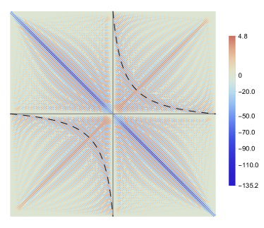
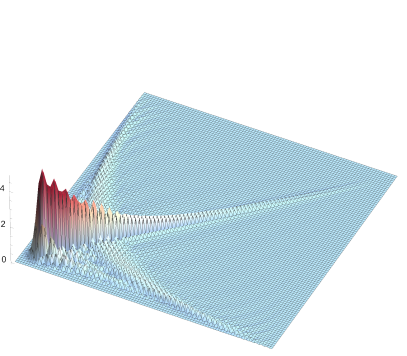
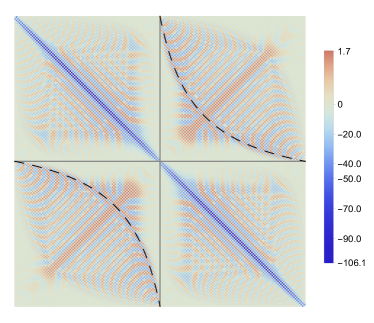
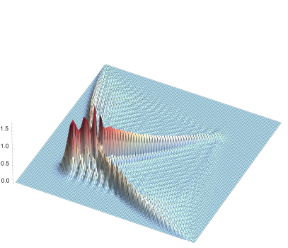
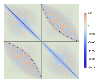
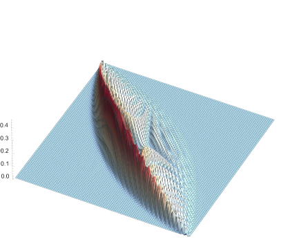
Figure 1: Left: Visualization of the matrix elements in $H$ for equal intervals of size $N=100$ and separations $21,51,101$, from top to bottom, with the color code representing the amplitudes. The four blocks in (18) are separated by grey lines, and the black dashed lines in the off-diagonal blocks indicate the hyperbolae $x_{\textrm{\tiny c}}(x)$ in (8). Right: 3D plots of the off-diagonal block $H^{\textrm{\tiny(1,2)}}$, with the absolute values of the matrix elements shown. The color coding differs from that on the left.

The novel feature is the structure in the off-diagonal blocks, which was visible in Ref. Arias_etal17_1 but not further studied there. According to the continuum results of Sec. II.1, the off-diagonal block should contain only single hopping terms between the conjugate sites, which lie on a hyperbola as indicated by the dashed black lines in Fig. 1. On the lattice one obtains a more complicated structure, however, one can still recognize the location of the hyperbolae from the color-coded plots. To better visualize the structure of the off-diagonal block, we also give 3D-plots on the right of Fig. 1, showing the absolute values of the matrix elements. Here the hyperbolic shape is even more evident, one has, however, an additional structure along the antidiagonal as the distance between the segments decreases. For large distances the hyperbola moves towards the diagonal and the structure becomes increasingly more peaked with decreasing amplitude.

One should emphasise that the dominant amplitudes in the diagonal blocks are two orders of magnitude larger than those in the off-diagonal ones. Furthermore, the former show an extensive scaling with $N$, as one would expect from the local weight function (12), which has a dimension of length. In contrast, the matrix elements in the off-diagonal block do not scale with $N$, as the corresponding bi-local weight (13) is dimensionless. However, in order to recover the functions $\beta(x)$ and $\tilde{\beta}(x)$ from the lattice data, one needs some further considerations. Indeed, it was already argued in Ref. Arias_etal17_1 that the longer-range hopping terms on the lattice should be included properly to recover the local weight function. Moreover, for a single interval the continuum limit can even be carried out analytically, recovering the CFT expression Eisler/Tonni/Peschel19 . In the following we shall demonstrate how the continuum limit works for the double interval, both for the local as well as bi-local weights.

IV Continuum limit

The continuum limit provides a relation between the entanglement Hamiltonian on the lattice and the one obtained for the Dirac fermion theory. It amounts to introduce a lattice spacing $s\to 0$ and consider the thermodynamic limit $N_{\sigma}\to\infty$ such that $N_{\sigma}s=\ell_{\sigma}$ is fixed, with $\sigma=1,2$. Due to the block structure (18) for the double interval, one should distinguish between the diagonal and off-diagonal blocks of the entanglement Hamiltonian. As expected, the former one shall reproduce the local kinetic term (1), whereas the latter one corresponds to the bi-local contribution (6).

We first consider the diagonal blocks and proceed similarly as in the case of a single interval Eisler/Tonni/Peschel19 . Namely, we rewrite the entanglement Hamiltonian as an inhomogeneous long-range hopping model

$$\mathcal{H}^{\textrm{\tiny$(\sigma)$}}=-\sum_{i\in A_{\sigma}}t_{0}(i)\,c_{i}^{\dagger}c_{i}-\sum_{i\in A_{\sigma}}\sum_{r\geq 1}t_{r}(i+r/2)\Big{(}c_{i}^{\dagger}c_{i+r}+c_{i+r}^{\dagger}c_{i}\Big{)}\,,$$ (19)

where the hopping amplitude satisfies

$$t_{r}(i+r/2)=\Bigg{\{}\,\begin{array}[]{ll}-H^{\textrm{\tiny$(\sigma)$}}_{i,i+r}&i,i+r\in A_{\sigma}\,,\\ 0&\mathrm{otherwise}\,.\end{array}$$ (20)

Note that the argument of the $r$-th neighbour amplitude corresponds to the midpoint of the sites involved and we assume it to vary slowly in the variable $i$. We then introduce the continuous coordinate $x=i\,s$, and apply the usual substitution for the fermion operators

$$c_{i}\;\longrightarrow\;\sqrt{s}\,\Big{(}e^{\textrm{i}q_{F}x}\,\psi_{\textrm{\tiny R}}(x)+e^{-\textrm{i}q_{F}x}\,\psi_{\textrm{\tiny L}}(x)\Big{)}\,,$$ (21)

thus rewriting them in terms of right- and left-moving fields. The phase factors are needed to account for the quick oscillations on the lattice. In turn, the substitution (21) amounts to linearizing the dispersion and shifting the Fermi points to $q=0$, thus reproducing the relativistic dispersion.

Carrying out the continuum limit is then rather straightforward. Substituting (21) into (19), Taylor expanding the fields as well as the hopping amplitude $t_{r}(i+r/2)\to t_{r}(x)+r\,s\,t_{r}^{\prime}(x)/2$ to first order in $s$, and dropping oscillatory terms, one arrives at the following expression Eisler/Tonni/Peschel19

$$\mathcal{H}^{\textrm{\tiny$(\sigma)$}}\;\longrightarrow\;\int_{A_{\sigma}}\textrm{d}x\,\Big{[}v(x)\,T_{00}(x)-\mu(x)\,N(x)\Big{]}\,,$$ (22)

where $T_{00}(x)$ is given by (3) and $N(x)$ is the number operator

$$N(x)=\psi^{\dagger}_{\textrm{\tiny R}}(x)\,\psi_{\textrm{\tiny R}}(x)+\psi^{\dagger}_{\textrm{\tiny L}}(x)\,\psi_{\textrm{\tiny L}}(x)\,,$$ (23)

while the functions $\mu(x)$ and $v(x)$ are defined as

$$v(x)\equiv\,2s\sum_{r=1}^{\infty}r\,\sin(rq_{F}s)\,t_{r}(x)\,,\;\qquad\;\mu(x)\equiv t_{0}(x)+2\sum_{r=1}^{\infty}\cos(rq_{F}s)\,t_{r}(x)\,.$$ (24)

The result (22) is an inhomogeneous Dirac theory with velocity parameter $v(x)$ and a chemical potential $\mu(x)$. Hence, contrary to naive expectations, the Fermi velocity in the continuum does not simply correspond to the nearest-neighbour hopping on the lattice, but is rather modified by the presence of long-range hopping. Furthermore, in order to get a finite result for the velocity $v(x)$, the hopping terms $t_{r}(x)$ should scale with the size $N_{\sigma}$ of the segment, which is indeed the case as pointed out in sec. III. In contrast to the single interval case Eisler/Peschel17 , however, we have no analytical results on $t_{r}(x)$ and the sums in (24) must be evaluated numerically. In particular, to recover the local piece $\mathcal{H}_{\textrm{\tiny loc}}=\mathcal{H}^{\textrm{\tiny(1)}}+\mathcal{H}^{\textrm{\tiny(2)}}$ one needs to find $v(x)=2\pi\beta(x)$ and $\mu(x)=0$.

Let us now consider the off-diagonal blocks in (18). Using the symmetry of the matrix, one could define the corresponding piece of the entanglement Hamiltonian as

$$\mathcal{H}^{\textrm{\tiny(1,2)}}\,=\,\frac{1}{2}\sum_{\begin{subarray}{c}i\in A_{1}\\ j\in A_{2}\end{subarray}}\!H^{\textrm{\tiny(1,2)}}_{i,j}\Big{(}c^{{\dagger}}_{i}c_{j}+c^{{\dagger}}_{j}c_{i}\Big{)}\,.$$ (25)

We would like to reproduce the bi-local term (6) by an appropriate continuum limit, we thus fix $is=x$ and look for the contributions around the conjugate site $js\approx x_{\textrm{\tiny c}}$. Since the matrix elements in the off-diagonal block do not scale with the segment size, it is enough to keep the zeroth order term in the expansion of the fields. This is given by

$$c_{i}^{\dagger}c_{j}+c^{{\dagger}}_{j}c_{i} \longrightarrow s\;\Big{[}\,\mathrm{e}^{\textrm{i}q_{F}s(j-i)}\psi^{\dagger}_{\textrm{\tiny R}}(x)\,\psi_{\textrm{\tiny R}}(x_{\textrm{\tiny c}})+\mathrm{e}^{-\textrm{i}q_{F}s(j-i)}\psi^{\dagger}_{\textrm{\tiny L}}(x)\,\psi_{\textrm{\tiny L}}(x_{\textrm{\tiny c}})$$ (26)

$$\hskip 5.69046pt+\,\mathrm{e}^{\textrm{i}q_{F}s(j+i)}\psi^{\dagger}_{\textrm{\tiny L}}(x)\,\psi_{\textrm{\tiny R}}(x_{\textrm{\tiny c}})+\mathrm{e}^{-\textrm{i}q_{F}s(j+i)}\psi^{\dagger}_{\textrm{\tiny R}}(x)\,\psi_{\textrm{\tiny L}}(x_{\textrm{\tiny c}})+\textrm{h.c.}\,\Big{]}\,.$$

Note that in the above expression each term has an oscillatory factor with a large argument. In fact, it is not clear a priori, which one of these term provides a proper continuum limit, i.e. a smooth function of $i$. Since for the infinite chain the left- and right-moving fermions are not supposed to mix, we will consider the exponentials with the $j-i$ factors and will provide further justification later. The bi-local piece of the entanglement Hamiltonian then reads

$$\mathcal{H}^{\textrm{\tiny(1,2)}}\;\longrightarrow\;\int_{A_{1}}\mathrm{d}x\,\Big{[}\,\mathcal{S}(x)\,T_{\textrm{\tiny bi-loc}}(x,x_{\textrm{\tiny c}})+\mathcal{C}(x)\,\tilde{T}_{\textrm{\tiny bi-loc}}(x,x_{\textrm{\tiny c}})\,\Big{]}\,,$$ (27)

where $T_{\textrm{\tiny bi-loc}}(x,x_{\textrm{\tiny c}})$ is the operator defined in (7) and

$$\tilde{T}_{\textrm{\tiny bi-loc}}(x,x_{\textrm{\tiny c}})=\frac{1}{2}\left[\,\psi^{\dagger}_{\textrm{\tiny R}}(x)\,\psi_{\textrm{\tiny R}}(x_{\textrm{\tiny c}})+\psi^{\dagger}_{\textrm{\tiny L}}(x)\,\psi_{\textrm{\tiny L}}(x_{\textrm{\tiny c}})+\textrm{h.c.}\,\right].$$ (28)

The corresponding weight functions with $x_{i}=i\,s$ are given by

$$\mathcal{S}(x_{i})=\sum_{j\in A_{2}}\sin[q_{F}s(j-i)]\,H^{\textrm{\tiny(1,2)}}_{i,j}\,,\;\;\qquad\;\;\mathcal{C}(x_{i})=\sum_{j\in A_{2}}\cos[q_{F}s(j-i)]\,H^{\textrm{\tiny(1,2)}}_{i,j}\,.$$ (29)

The same procedure can be carried out for the piece $\mathcal{H}^{\textrm{\tiny(2,1)}}$ with indices $i$ and $j$ in (25) interchanged. The continuum limit is the same as (27) with the integral running over $A_{2}$, and the sums in (29) running over $A_{1}$.

IV.1 Equal intervals at half filling

We start with the simplest case of equal intervals $N_{1}=N_{2}=N$ at half filling $q_{F}\,s=\pi/2$, setting $A_{2}=\left[d+1,d+N\right]$ and $A_{1}=\left[-(d+N),-(d+1)\right]$ such that the distance between the intervals is $2d+1$. The coordinates of the endpoints in the continuum description must be chosen as $a=ds$ and $b=(d+N)s$, such that $b-a=\ell$. Due to particle-hole symmetry, $H$ has a checkerboard structure with $H_{i,i+2p}=0$, which immediately yields $\mu(x)=0$, whereas $v(x)$ has to be determined numerically. Due to the extensive scaling of the diagonal blocks, it is useful to introduce the rescaled hopping

$$h_{i-p,i+p+1}=-H_{i-p,i+p+1}/N=\,t_{2p+1}(i)/N\,.$$ (30)

Using this in (24) with $x_{i}=i\,s$ and fixing the scale as $Ns=\ell=1$, the velocity reads

$$v(x_{i})=2\sum_{p=0}^{P}(-1)^{p}\,(2p+1)\,h_{i-p,i+p+1}\,,$$ (31)

where we introduced a cutoff $P<N/2$. Note that for a fixed $i\in\left[d+1,d+N-1\right]$ the sums are carried out perpendicular to the main diagonal of the matrix.

The convergence of $v(x_{i})$ as a function of the cutoff is shown in Fig. 2 for $N=80$ and $d=10,20$. The case $P=0$ is simply the scaled nearest-neighbour hopping and one observes that as the distance between the segments becomes smaller, it deviates more and more from the continuum limit prediction $2\pi\beta(i/N)$, shown by the red lines. Indeed, the data for $P=0$ lies well above the red line with its maximum shifted towards the center of the chain, and a good overlap is found only close to the boundaries. Increasing the value of $P$ one finds a slow convergence towards the continuum limit and already for $P=10$ one has an almost perfect overlap.

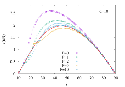
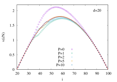
Figure 2: Convergence of the velocity parameter (31) in the continuum limit of the entanglement Hamiltonian for a double interval with $N=80$ and $d=10,20$. The red solid line shows the function $2\pi\beta(i/N)$ from (12) setting $a=d/N$ and $b=1+d/N$. Note that the figures always show the right segment.

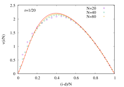
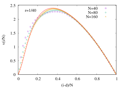
Figure 3: Convergence of $v(x_{i})$ for a fixed ratio $r=d/N$ and increasing values of $N$, plotted against $(i-d)/N$. The red solid lines show the weight function $2\pi\beta(r+y)$ in (12) as a function of $y$, setting $a=r$ and $b=1+r$.

In the above examples the ratio $r=d/N$ between the distance and segment size is large enough to ensure a very good convergence already for moderate $N$. The situation becomes more complicated for small ratios $r$, as shown in Fig. 3. Here the velocity $v(x_{i})$ is calculated using the maximal cutoff $P=N/2-1$ for various $d$ and $N$, keeping their ratio fixed. One finds that for $r=1/20$ already $N=80$ is sufficient to converge the data, whereas for $r=1/40$ the data set $N=160$ still shows some visible deviations. Obviously, this is because the number of sites $2d+1=9$ between the segments is still too small to ensure a reasonable continuum limit. Nevertheless, Fig. 3 convincingly demonstrates that the limit is approached smoothly for $N\to\infty$.

Finally, we consider the off-diagonal scaling functions in (29). Note that here the range of the lattice variable is $i\in\left[d+1,d+N\right]$ and we chose $a=ds$ and $b=(d+N)s$ for the boundaries in the continuum case. Since the weight function must vanish exactly at $x=b$, it is useful to slightly shift the discretized coordinates $x_{i}=(i-1/2)s$ to get a better overlap with the continuum results. At half filling the function $\mathcal{C}(x_{i})=0$ vanishes identically, while $\mathcal{S}(x_{i})$ simplifies to

$$\mathcal{S}(x_{i})=\sum_{j\in A_{1}}(-1)^{(j-i-1)/2}H_{i,j}\,,\;\;\;\;\qquad\;\;\;\;x_{i}\in(a,b)\,.$$ (32)

In contrast to the local term, this definition involves an alternating row-wise sum of the matrix elements. The result is shown in Fig. 4 for increasing segment sizes $N$ and fixed ratios $r=1/5$ and $r=1/10$. In both cases one obtains a very good convergence towards the bi-local weight $2\pi\tilde{\beta}(x)$, shown by the red lines. This function is more concentrated near the left end of the segment than $2\pi\beta(x)$ due to the factor $1/x$ in (13), and the effect increases for smaller distances. Note that the relation $\mathcal{S}(-x_{i})=-\,\mathcal{S}(x_{i})$ follows by symmetry arguments. One should also remark that keeping the terms in (26) with $i+j$ would lead to another sum that is simply related to (32) by $(-1)^{i}\mathcal{S}(x_{i})$. Obviously, this is an alternating expression which vanishes in the continuum limit, thus justifying our choice of dropping these terms.

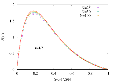
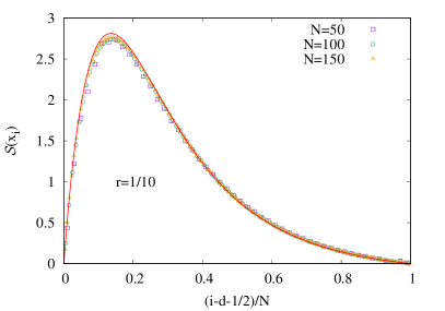
Figure 4: Bi-local weight function $\mathcal{S}(x_{i})$ at half filling for increasing segment sizes $N$ and two different ratios $r=d/N$, shown against the variable $x_{i}-r$. The red lines show the continuum result $2\pi\tilde{\beta}(x)$ for comparison.

IV.2 Arbitrary filling

We now move to the case of arbitrary filling, choosing equal intervals for simplicity. For a single interval one can actually show analytically, that the continuum limit leads to the exact same expressions as in the half-filled case Eisler/Tonni/Peschel19 . This proof uses the analytical expressions for $t_{r}(x)$, which are nonzero for both even and odd $r$ Eisler/Peschel17 , to evaluate the sums in (24). In the present case, where the sums are carried out numerically, this leads to some complications as the hopping profiles (20) on the lattice are associated to integer and half-integer sites for even and odd $r$, respectively. Thus, analogously to the odd sums as in (31) for the half-filled case, one could define an even sum, albeit with coordinates assigned as $x_{i}=(i-1/2)s$. The even and odd sums can then be added by summing the $i$-th term of the odd sequence with the average of the $i$-th and $(i+1)$-th terms of the even sequence. Alternatively, one could also define the row-wise sums with $x_{i}=(i-1/2)s$

$$v(x_{i})\,=\!\sum_{j\in A_{2}}\sin[q_{F}s(j-i)]\,(j-i)h_{i,j}\,,\;\;\;\qquad\;\;\;\mu(x_{i})\,=\,-\!\sum_{j\in A_{2}}\cos[q_{F}s(j-i)]\,H_{i,j}\,,$$ (33)

which also give only corrections of order $s^{2}$ that vanish in the continuum limit. Note that the factor of two as compared to (24) is now missing, since the sums run over an entire row of the matrix and not only in the upper diagonal part.

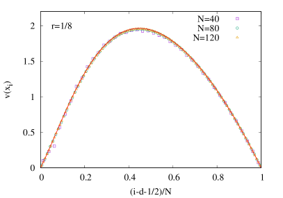
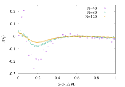
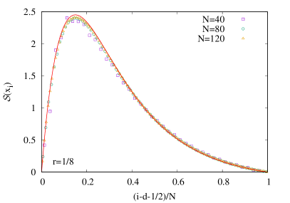
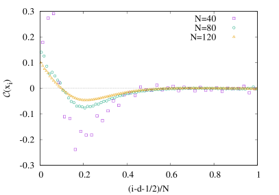
Figure 5: Top panel: velocity $v(x_{i})$ (left) and chemical potential $\mu(x_{i})$ (right) from (33) at $1/3$ filling with a ratio $r=1/8$. The red solid line shows the result $2\pi\beta(x)$. Bottom panel: bi-local weight functions $\mathcal{S}(x_{i})$ (left) and $\mathcal{C}(x_{i})$ (right) from (29). The red solid line shows the result $2\pi\tilde{\beta}(x)$.

We observed that the row-wise sums yield a smoother convergence towards the expected weight functions. This is essentially due to the large oscillations as a function of $i$ in the even/odd diagonal sums, which do not cancel perfectly when following the averaging process described above. The row-wise sums (33) are shown in the top panel of Fig. 5 for $1/3$ filling (corresponding to $q_{F}s=\pi/3$) for a ratio $r=1/8$ and increasing $N$. For $v(x_{i})$ on the left hand side, the convergence towards $2\pi\beta(x)$ is excellent already for the moderate segment sizes used. The chemical potential on the right shows a much slower convergence towards zero. However, this is a result of rather nontrivial cancellations in the sums (33), since the definition of $\mu(x_{i})$ involves the unscaled $H_{i,j}$. We also show the results for the bi-local weight functions (29), given by row-wise sums for generic fillings, in the bottom panel of Fig. 5. The comparison of $\mathcal{S}(x_{i})$ against $2\pi\tilde{\beta}(x)$ shows a very good agreement, with only tiny deviations visible around the maximum. Similarly to $\mu(x_{i})$, the bi-local weight $\mathcal{C}(x_{i})$ defined with the cosine function goes towards zero as it should.

IV.3 Unequal intervals

As a final example, we discuss the case of unequal intervals in a half-filled chain. Due to translational invariance, one can make the choice $A_{1}=\left[1,N_{1}\right]$ and $A_{2}=\left[N_{1}+D+1,N_{1}+D+N_{2}\right]$ for the intervals of size $N_{1}$ and $N_{2}$, separated by $D$ sites. The matrix plot in Fig. 6 shows that the main features are similar to the symmetric case, and the hyperbola $x_{\textrm{\tiny c}}(x)$ can again be recognized. However, the fine structure in the off-diagonal block differs from the one in Fig. 1, with a curved structure appearing also along the antidiagonal.

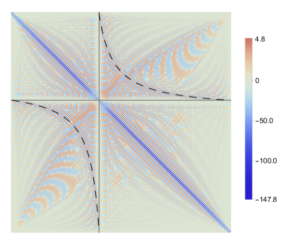
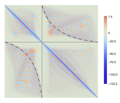
Figure 6: Matrix elements in $H$ for the case of unequal segments with $N_{1}=80$, $N_{2}=120$ and $D=21$ (left) and $51$ (right).

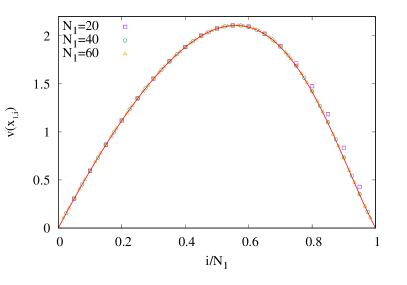
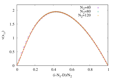
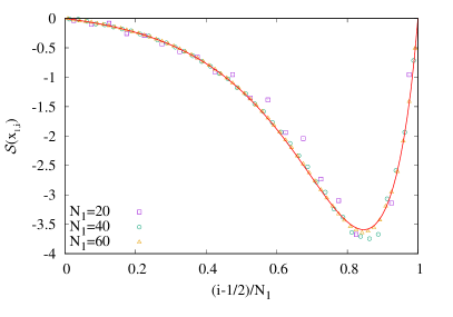
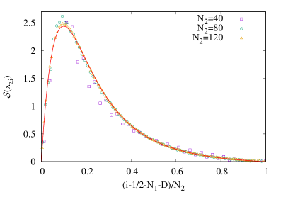
Figure 7: Continuum limit for unequal intervals. Top panel: $v(x_{\sigma,i})$ for the left and right intervals, respectively, compared to $2\pi\beta(x)$. Bottom panel: $\mathcal{S}(x_{\sigma,i})$ for the left and right intervals, compared to $2\pi\tilde{\beta}(x)$. The data is shown for various segment sizes, with the ratios $N_{1}/N_{2}=1/2$ and $D/N_{2}=1/8$ kept fixed.

Clearly, there are now two scales in the problem and by taking the continuum limit one has to fix $N_{\sigma}s=\ell_{\sigma}$, with the boundary coordinates given by $a_{1}=0$, $b_{1}=N_{1}s$, $a_{2}=(N_{1}+D)s$ and $b_{2}=(N_{1}+N_{2}+D)s$. Furthermore, the diagonal blocks also scale with the corresponding segment size and the densities can be introduced as

$$h^{\textrm{\tiny$(\sigma)$}}_{i-p,i+p+1}\,=\,-\,H^{\textrm{\tiny$(\sigma)$}}_{i-p,i+p+1}/N_{\sigma}\,.$$ (34)

However, the quantities $\beta(x)/\ell_{\sigma}$ and $\tilde{\beta}(x)$ are dimensionless and scale invariant, i.e. they remain unchanged under a rescaling of each length in the functions. This property can be used to fix either the length scale $\ell_{1}=1$ for the left interval or $\ell_{2}=1$ for the right one, leading to the definition

$$v(x_{\sigma,i})=2\sum_{p=0}^{P}(-1)^{p}(2p+1)\,h^{\textrm{\tiny$(\sigma)$}}_{i-p,i+p+1}\,,\;\;\;\qquad\;\;\;x_{\sigma,i}=i/N_{\sigma}\,.$$ (35)

The parameters of the corresponding $\beta(x)$ function must be scaled accordingly, and can be shown to depend only on the two ratios $\nu=N_{1}/N_{2}$ and $r=D/N_{2}$. In particular, for the right interval one has $a_{1}=0$, $b_{1}=\nu$, $a_{2}=\nu+r$ and $b_{2}=\nu+r+1$, whereas the parameters for the left interval read $a_{1}=0$, $b_{1}=1$, $a_{2}=1+r/\nu$ and $b_{2}=1+(1+r)/\nu$. The same arguments apply also for the bi-local weight, which is defined analogously to (32), with arguments $x_{\sigma,i}=(i-1/2)/N_{\sigma}$.

The scaling functions of the local $v(x_{\sigma,i})$ and bi-local $\mathcal{S}(x_{\sigma,i})$ weights are shown in Fig. 7 for increasing segment sizes, keeping the ratios $\nu=1/2$ and $r=1/8$ fixed. The results for the right interval are shifted such that they also fall within the interval $(0,1)$. As in the previous examples, one can see a very good convergence towards the expected continuum result. The only sizable deviations occur for the shortest segments considered, corresponding to a distance of only $D=5$ lattice sites. It is straightforward to generalize the calculation to arbitrary fillings, where one obtains again a very good agreement with the same weight functions.

V Interval on the half line

Another important example where the entanglement Hamiltonian takes the form (5) corresponds to the bipartition of the half line $x\geqslant 0$ where $A=(a,b)$ is an interval in a generic position.

V.1 Continuum results

For the massless Dirac field, the most general boundary condition ensuring the global energy conservation corresponds to imposing the vanishing of the energy flow, $T_{10}(x=0)=0$, through the boundary Cardy84 ; Cardy86 ; Cardy89 . This boundary condition can be satisfied in two inequivalent ways, corresponding to a vector and an axial $U(1)$ symmetry Liguori/Mintchev98 . Here we discuss only the former case, which corresponds to the following boundary condition on the fields

$$\psi_{\textrm{\tiny R}}(0)=\textrm{e}^{\textrm{i}\alpha}\,\psi_{\textrm{\tiny L}}(0)\,,$$ (36)

with a scattering phase $\alpha\in[0,2\pi)$. Thus, the boundary condition at $x=0$ provides a scale invariant coupling of the fields having different chirality.

The entanglement Hamiltonian of an interval $A=(a,b)$ on the half line $x\geqslant 0$ has been found in Mintchev/Tonni21 and it takes the form (5). In particular, the local term is still given by (1) with the weight function (12) and the energy density $T_{00}$ defined in (3). Instead, the bi-local term in (5) is

$$\mathcal{H}_{\textrm{\tiny bi-loc}}\,=\,2\pi\int_{a}^{b}\textrm{d}x\,\tilde{\beta}(x)\,T_{\textrm{\tiny bi-loc}}(x,\tilde{x};\alpha)\,,$$ (37)

where the weight function coincides with (13), but the bi-local operator is defined as

$$T_{\textrm{\tiny bi-loc}}(x,\tilde{x};\alpha)\equiv\frac{\textrm{i}}{2}\;\!:\!\!\Big{[}\,\textrm{e}^{\textrm{i}\alpha}\,\psi^{\dagger}_{\textrm{\tiny R}}(x)\,\psi_{\textrm{\tiny L}}(\tilde{x})-\textrm{e}^{-\textrm{i}\alpha}\,\psi^{\dagger}_{\textrm{\tiny L}}(x)\,\psi_{\textrm{\tiny R}}(\tilde{x})+\textrm{h.c.}\,\Big{]}\!\!:\;,$$ (38)

which depends on the phase occurring in the boundary condition (36), and $\tilde{x}=ab/x$ is the point conjugate to $x$ inside $A$. It is related to the conjugate point (8) for two disjoint intervals in the symmetric configuration where $(a_{1},b_{1})=(-b,-a)$ and $(a_{2},b_{2})=(a,b)$.

V.2 Lattice results

Consider now the lattice model given by a semi-infinite fermionic hopping chain, whose Hamiltonian is (14) with the sums over $n$ restricted to $n\geqslant 1$, and the subsystem $A=\left[d+1,d+N\right]$ made by $N$ consecutive sites and separated by $d$ sites from the boundary of the chain. The open half-chain is the simplest realization of the Dirac theory with a boundary, corresponding to the choice $\alpha=\pi$. As suggested by the continuum results above, the entanglement Hamiltonian should be very closely related to the case of the symmetric double interval. We first derive the exact correspondence on the lattice level.

Let us consider the symmetric double interval on the infinite chain, composed of $A_{2}=\left[d+1,d+N\right]$ and its reflection to negative sites $A_{1}=\left[-\,d-N,-\,d-1\right]$, as in Sec. IV.1. The eigenvalues $\zeta_{k}$ and eigenvectors $\phi_{k}$ of the $2N\times 2N$ reduced correlation matrix with elements (17) then follow from the equations

$$\begin{array}[]{l}C_{i^{\prime},\,j^{\prime}}\,\phi^{\textrm{\tiny(1)}}_{k}(j^{\prime})+C_{i^{\prime},j}\,\phi^{\textrm{\tiny(2)}}_{k}(j)\,=\,\zeta_{k}\,\phi^{\textrm{\tiny(1)}}_{k}(i^{\prime})\,,\\ C_{i,\,j^{\prime}}\,\phi^{\textrm{\tiny(1)}}_{k}(j^{\prime})+C_{i,j}\,\phi^{\textrm{\tiny(2)}}_{k}(j)\,=\,\zeta_{k}\,\phi^{\textrm{\tiny(2)}}_{k}(i)\,,\end{array}$$ (39)

where $i,j\in A_{2}$ and $i^{\prime},j^{\prime}\in A_{1}$ and the $k$-th eigenvector has been decomposed into two vectors corresponding to amplitudes on the left/right interval, respectively:

$$\phi_{k}=\Bigg{(}\begin{array}[]{c}\phi^{\textrm{\tiny(1)}}_{k}\\ \phi^{\textrm{\tiny(2)}}_{k}\end{array}\Bigg{)}\,.$$ (40)

Due to the reflection symmetry of the geometry, the eigenvectors are either even or odd, $\phi^{\textrm{\tiny(1)}}_{k}(-i)=\pm\phi^{\textrm{\tiny(2)}}_{k}(i)$. Using this property and introducing $j^{\prime}=-j$, $i^{\prime}=-i$, the eigenvalue equations (39) can be decomposed into two sets

$$C^{\pm}_{i,j}\phi^{\textrm{\tiny(2)}}_{k}(j)\,=\,\zeta^{\pm}_{k}\,\phi^{\textrm{\tiny(2)}}_{k}(j)\,,$$ (41)

where the $N\times N$ correlation matrices $C^{\,\pm}$ with elements $i,j\in A_{2}$ are defined as

$$C^{\pm}_{i,j}=\frac{\sin[q_{\textrm{\tiny F}}(i-j)]}{\pi(i-j)}\pm\frac{\sin[q_{\textrm{\tiny F}}(i+j)]}{\pi(i+j)}\,.$$ (42)

In fact, the piece containing $i+j$ originates from the terms $C_{i,-j}$ and $C_{-i,j}$ in (39) after making the above substitutions, whereas $C_{-i,\,-j}=C_{i,j}$. Note that the above observations are independent of the distance $d$.

Remarkably, the correlation matrices $C^{\pm}$ in (42) are nothing but the ones corresponding to a half-chain with Dirichlet or Neumann boundary conditions. They can be obtained by replacing the plane-wave basis of the infinite chain with appropriate standing-wave bases as

$$C^{+}_{i,j}=\frac{2}{\pi}\int_{0}^{q_{\textrm{\tiny F}}}\!\cos(q\,i)\,\cos(q\,j)\,\textrm{d}q\,,\;\;\qquad\;\;C^{-}_{i,j}=\frac{2}{\pi}\int_{0}^{q_{\textrm{\tiny F}}}\!\sin(q\,i)\,\sin(q\,j)\,\textrm{d}q\,.$$ (43)

Hence, the eigenvalue equation (41) simply tells us, that the even/odd eigenvectors and corresponding eigenvalues of the double interval problem are, up to normalization, identical to the ones for the half-chain with Dirichlet/Neumann boundary conditions.

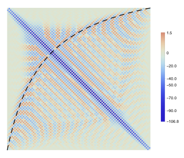
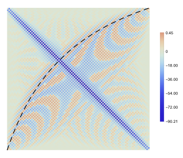
Figure 8: Entanglement Hamiltonian matrix for a block of consecutive sites in the semi-infinite chain with Dirichlet boundary conditions and at half filling. Left: $(d,N)=(25,100)$. Right: $(d,N)=(50,100)$. The panels should be compared to the middle and bottom panel on the left of Fig. 1.

The above observations can be used directly in the entanglement Hamiltonians $H^{\pm}$ of the chains with corresponding boundary conditions. These are defined analogously to (16) as

$$H^{\pm}_{i,j}=2\sum_{k=1}^{N}\,\phi^{\pm}_{k}(i)\;\varepsilon^{\pm}_{k}\;\phi^{\pm}_{k}(j)\,,\;\;\;\;\qquad\;\;\;\;i,j\in A_{2}\,,$$ (44)

such that they are composed of only the even/odd eigenvectors $\phi^{\pm}_{k}$ of the double interval problem, with the factor two resulting from the different normalization. Comparing now to the block matrix (18), one can see immediately that $H^{+}_{i,j}+H^{-}_{i,j}=2H^{\textrm{\tiny(2)}}_{i,j}$, as well as $H^{+}_{i,j}-H^{-}_{i,j}=2H^{\textrm{\tiny(2,1)}}_{i,-j}$. In other words, the entanglement Hamiltonians for the half-chain with Dirichlet/Neumann boundary conditions can be written as

$$H^{\pm}_{i,j}=H^{\textrm{\tiny(2)}}_{i,j}\pm{H}^{\textrm{\tiny(2,1)}}_{i,-j}\;,$$ (45)

in terms of the diagonal and off-diagonal blocks in the symmetric double interval.

In Fig. 8 we show $H^{-}$ corresponding to a block of $N=100$ sites and for two different values of the distance $d$ from the boundary of the open semi-infinite chain, in the special case of half filling. These plots should be compared to the middle and bottom left panels of Fig. 1, displaying the symmetric double interval with the corresponding $d$. One can immediately recognize that the matrix $H^{-}$ for the open half-chain is indeed a kind of superposition of the diagonal and off-diagonal blocks for the double interval, as dictated by (45). In particular, one can see that the hyperbola is now reflected and appears at $\tilde{x}=ab/x$, as shown by the black dashed lines in Fig. 8.

The result (45) already makes it clear that the relation between the half-chain problem and the double interval is completely analogous to the continuum case in sec. V.1. However, it remains to understand the difference between the bi-local operators (38) and (7), by considering the continuum limit of $H^{\pm}$. We first apply the substitutions (21), where the left/right-moving fields are coupled via the boundary condition (36) at $x=0$. This coupling can be made explicit by writing the mode expansion of the fields $\psi_{\textrm{\tiny L}}(x)$ and $\psi_{\textrm{\tiny R}}(x)$, where the parameter $\alpha$ enters as a relative phase between the left/right propagating Fourier components. In our case here $H^{+}$ and $H^{-}$ correspond to the choice $\alpha=0$ and $\alpha=\pi$, respectively. The change of the bi-local operator is due to the fact that the corresponding matrix component in (45) is mirrored. As pointed out already below (26), it is not a priori clear which phase factors give a proper continuum limit in this expansion. Due to the appearance of ${H}^{\textrm{\tiny(2,1)}}_{i,-j}$, it is now clear that for the half-chain one has to choose the terms with $i+j$. This leads to the following expression

$$\mathcal{H}^{\pm}_{\textrm{\tiny bi-loc}}=\pm\int_{A}\mathrm{d}x\,\Big{[}\,\mathcal{C}(x)\,T_{\textrm{\tiny bi-loc}}^{\textrm{\tiny$(1)$}}(x,\tilde{x})+\mathcal{S}(x)\,T_{\textrm{\tiny bi-loc}}^{\textrm{\tiny$(2)$}}(x,\tilde{x})\,\Big{]}\,,$$ (46)

where the operators are defined as

$$T_{\textrm{\tiny bi-loc}}^{\textrm{\tiny$(1)$}}(x,\tilde{x}) = \frac{1}{2}\left[\,\psi^{\dagger}_{\textrm{\tiny R}}(x)\,\psi_{\textrm{\tiny L}}(\tilde{x})+\psi^{\dagger}_{\textrm{\tiny L}}(x)\,\psi_{\textrm{\tiny R}}(\tilde{x})+\textrm{h.c.}\,\right],$$ (47)

$$\rule{0.0pt}{19.91684pt}T_{\textrm{\tiny bi-loc}}^{\textrm{\tiny$(2)$}}(x,\tilde{x}) = \frac{\mathrm{i}}{2}\left[\,\psi^{\dagger}_{\textrm{\tiny R}}(x)\,\psi_{\textrm{\tiny L}}(\tilde{x})-\psi^{\dagger}_{\textrm{\tiny L}}(x)\,\psi_{\textrm{\tiny R}}(\tilde{x})+\textrm{h.c.}\,\right],$$ (48)

and the bi-local weights are given by

$$\mathcal{C}(x_{i})=\sum_{j\in A}\cos[q_{F}s(j+i)]\,H^{\textrm{\tiny(2,1)}}_{i,-j}\;,\;\;\;\qquad\;\;\;\mathcal{S}(x_{i})=-\sum_{j\in A}\sin[q_{F}s(j+i)]\,H^{\textrm{\tiny(2,1)}}_{i,-j}\;.$$ (49)

Interchanging $j\to-j$, one clearly arrives at the same definition of the weights as in (29) for the double interval. Hence, in the limit $N\to\infty$, one has $\mathcal{S}(x_{i})\to 2\pi\tilde{\beta}(x)$ as well as $\mathcal{C}(x_{i})\to 0$, perfectly reproducing the result (37)-(38) for the boundary Dirac theory with $\alpha=0,\pi$.

The case $0<\alpha<\pi$ can also be studied on the lattice by introducing a chemical potential at the first site, i.e. adding the term $\mu_{1}c_{1}^{\dagger}c_{1}$ to the Hamiltonian with $\mu_{1}>0$. The eigenvectors are then cosine functions with a phase shift

$$\Phi(n)=\sqrt{\frac{2}{\pi}}\cos[qn+\delta(q)]\,,\;\;\;\qquad\;\;\;\tan\delta(q)=\frac{1+2\mu_{1}\cos q}{2\mu_{1}\sin q}\,.$$ (50)

The parameter of the continuum theory then corresponds to the relative phase at the Fermi level, $\alpha=2\delta(q_{F})$. It is easy to see that the correlation matrix has the form

$$C^{\alpha}_{i,j}=\frac{\sin[q_{\textrm{\tiny F}}(i-j)]}{\pi(i-j)}+\int_{0}^{q_{F}}\frac{\mathrm{d}q}{\pi}\cos[q(i+j)+2\delta(q)]\,,$$ (51)

and the corresponding $H^{\alpha}$ can be evaluated numerically. However, in contrast to (45), for generic $\alpha$ it is not clear how to separate the local and bi-local contributions that are superimposed in the matrix $H^{\alpha}$.

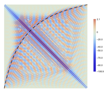
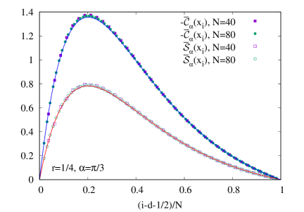
Figure 9: Left: matrix plot for $d=25$, $N=100$ and $\alpha=\pi/3$. Right: bi-local weights from (53) for ratio $r=d/N=1/4$ and $\alpha=\pi/3$. The red and blue lines show the expected continuum limit results in (54).

Here we propose such a method for the half-filled case. Inserting the full matrix into the definition of the bi-local weights,

$$\mathcal{C}_{\alpha}(x_{i})=\sum_{j\in A}\cos\!\big{(}\tfrac{\pi}{2}(j+i)\big{)}\,H^{\alpha}_{i,j}\,,\;\;\;\qquad\;\;\;\mathcal{S}_{\alpha}(x_{i})=-\sum_{j\in A}\sin\!\big{(}\tfrac{\pi}{2}(j+i)\big{)}\,H^{\alpha}_{i,j}\,,$$ (52)

the local contribution in $H^{\alpha}_{i,j}$ does not yield a proper continuum limit, since the sum contains the phase factors with $i+j$. Indeed, one can argue that this term has an alternating form $(-1)^{i}f(x_{i})$ with some smooth function $f(x_{i})$. In order to get rid of this unwanted contribution, we define

$$\bar{\mathcal{S}}_{\alpha}(x_{i})=\mathcal{S}_{\alpha}(x_{i})/2+\big{[}\mathcal{S}_{\alpha}(x_{i-1})+\mathcal{S}_{\alpha}(x_{i+1})\big{]}/4\;,$$ (53)

and similarly for $\bar{\mathcal{C}}_{\alpha}(x_{i})$. In other words, we combine the terms $i$ and $i\pm 1$, such that the alternating piece cancels up to second order corrections in the lattice spacing. In order to reproduce the continuum result, one expects

$$\bar{\mathcal{C}}_{\alpha}(x_{i})\,\to\,-\,2\pi\sin(\alpha)\,\tilde{\beta}(x)\,,\;\;\;\qquad\;\;\;\bar{\mathcal{S}}_{\alpha}(x_{i})\,\to\,2\pi\cos(\alpha)\,\tilde{\beta}(x)\,,$$ (54)

to hold. For a generic scattering phase $\alpha$, the checkerboard structure of the matrix $C^{\alpha}$ in (51) as well as of $H^{\alpha}$ is lost, and both of the sums in (52) are nonzero. This is demonstrated in Fig. 9, where we show the results for $\alpha=\pi/3$ by choosing the value of $\mu_{1}$ accordingly. The matrix plot on the left is more blurred due to the presence of nonzero elements $H^{\alpha}_{i,j}$ with even $j-i$, and on the right one can see a very good convergence towards (54) for both bi-local weight factors. We note that the local weights can be extracted analogously, inserting $H^{\alpha}$ into (33) and then defining the averages which now kill the bi-local contributions. As expected, we find $\bar{v}_{\alpha}(x_{i})\to 2\pi\beta(x_{i})$ and $\bar{\mu}_{\alpha}(x_{i})\to 0$ independently of $\alpha$.

VI Commuting operators

In the following we consider the integral operators whose kernels are the correlation functions restricted to a subsystem $A$ and discuss differential operators that commute with them.

VI.1 Single interval

We consider a single interval $A=(a,b)$ when the entire system is either on the line and in its ground state, or on the circle and in its ground state, or on the line and in a thermal state.

The integral operator associated with the correlation function $G(x,y)$ restricted to $A$ is

$$\mathcal{I}_{A}[f](x)\equiv\int_{A}\textrm{d}y\;G(x,y)\,f(y)\,,$$ (55)

and depends both on $G(x,y)$ and on the spatial domain. Consider now the following first-order differential operator

$$\mathcal{D}_{A}\equiv t(x)\,\frac{d}{dx}+\frac{1}{2}\,t^{\prime}(x)\,,$$ (56)

with a function $t(x)$ still to be determined and evaluate the action of the operators (55) and (56) on a generic function $f$ in the two possible orders, namely

$$\mathcal{D}_{A}\,\mathcal{I}_{A}[f](x)\,=\int_{A}\textrm{d}y\big{[}\mathcal{D}_{A,x}\,G(x,y)\big{]}f(y)\,=\int_{A}\textrm{d}y\left[t(x)\,\frac{d}{dx}G(x,y)+\frac{1}{2}\,t^{\prime}(x)\,G(x,y)\right]f(y)\,,$$ (57)

and

$$\mathcal{I}_{A}\big{[}\mathcal{D}_{A}f\big{]}(x)\,=\int_{A}\textrm{d}y\left\{-\,\frac{d}{dx}\big{[}G(x,y)\,t(y)\big{]}+\frac{1}{2}\,G(x,y)\,t^{\prime}(y)\right\}f(y)\,=\,-\int_{A}\textrm{d}y\big{[}\mathcal{D}_{A,y}\,G(x,y)\big{]}f(y)\,,$$ (58)

with $\mathcal{D}_{A,x}$ denoting the operator (56), while $\mathcal{D}_{A,y}$ is (56) written in terms of the variabile $y$ instead of $x$. In (58), an integration by parts has been performed with the assumption that $t(x)$ vanishes at the endpoints of $A$, i.e.

$$t(a)=t(b)=0\,.$$ (59)

One then sees that the operators (55) and (56) commute

$$\big{[}\,\mathcal{I}_{A}\,,\mathcal{D}_{A}\,\big{]}\,=\,0\,,$$ (60)

provided that

$$\big{(}\mathcal{D}_{A,x}+\mathcal{D}_{A,y}\big{)}G(x,y)=0\,.$$ (61)

Consider now the case of an infinite line with the system in its ground state. Then the kernel is given by (4)

$$G(x,y)=\frac{\textrm{i}}{x-y}\,,$$ (62)

and the condition (61) becomes explicitly

$$\frac{t(x)-t(y)}{(x-y)^{2}}-\frac{t^{\prime}(x)+t^{\prime}(y)}{2(x-y)}=0\,.$$ (63)

This functional equation is satisfied by an arbitrary quadratic function $t(x)$. The boundary condition (59) then gives, up to a prefactor,

$$t(x)=(x-a)(b-x)\,.$$ (64)

For this choice of $t(x)$, the differential operator (56) commutes with the integral kernel and thus has the same eigenfunctions. We note that $t(x)$ is proportional to the quantity $\beta(x)$ appearing in the entanglement Hamiltonian (1).

With this result, one can easily obtain the solution for a system on a circle with circumference $L$ in its ground state. The kernel then is

$$G(x,y)=\frac{\textrm{i}}{\sin[\pi(x-y)/L]}\,,$$ (65)

and one can check that the generalization of (64) to sine functions

$$t(x)=\sin[\pi(x-a)/L]\,\sin[\pi(b-x)/L]\,,$$ (66)

again satisfies (61). Finally, if the system is on a line but in a thermal state with inverse temperature $\beta$, one has

$$G(x,y)=\frac{\textrm{i}}{\sinh[\pi(x-y)/\beta]}\,,$$ (67)

and (61) holds if one substitutes hyperbolic sine functions in (64)

$$t(x)=\sinh[(x-a)/\beta]\,\sinh[(b-x)/\beta]\,.$$ (68)

The common eigenfunctions of $\mathcal{I}_{A}$ and $\mathcal{D}_{A}$ are easy to obtain from $\mathcal{D}_{A}$, since this is a first-order differential operator. In all three cases one has

$$\phi_{s}(x)\,=\,C\,\,\frac{\textrm{e}^{\textrm{i}sw(x)}}{\sqrt{t(x)}}\,,$$ (69)

with eigenvalue $\textrm{i}s$ and $w(x)$ given by

$$w(x)=\int\frac{\textrm{d}x}{t(x)}\,.$$ (70)

For $t(x)$ given by (64), $w(x)$ is proportional to $\ln[(x-a)/(b-x)]$ and the exponential factor describes the logarithmic oscillations found previously in Peschel04 ; Arias_etal17_1 .

VI.2 Modular flow

It was noted above that the function $t(x)$ in (64) is proportional to the weight factor $\beta(x)$ in the entanglement Hamiltonian. In fact, the whole operator $\mathcal{D}_{A}$ of the previous subsection also occurs in connection with $\mathcal{H}$, namely in the analysis of the modular flow of the chiral components of the massless Dirac field. This is their unitary evolution via the (modular) Hamiltonian $\mathcal{H}$ according to

$$\psi(x,\tau)\equiv\,\textrm{e}^{-\textrm{i}\mathcal{H}\tau}\,\psi(x)\,\textrm{e}^{\textrm{i}\mathcal{H}\tau}\,,$$ (71)

where $\psi(x)$ corresponds to the field operator at $\tau=0$ and we dropped the index $R,L$ at $\psi(x)$.

The equation of motion then is

$$\textrm{i}\,\partial_{\tau}\psi(x,\tau)=\left[\,\mathcal{H},\psi(x,\tau)\right]\,,$$ (72)

and inserting the expression for $\mathcal{H}$ given in (1) leads to the partial differential equation Casini/Huerta09 ; Mintchev/Tonni21

$$\frac{1}{2\pi}\,\partial_{\tau}\psi(x,\tau)\,=\,\pm\,\mathcal{D}_{A}\,\psi(x,\tau)\,,$$ (73)

where $\mathcal{D}_{A}$ is given by (56) with $t(x)\equiv\beta(x)$ and $\pm$ corresponds to the right and left chirality, respectively. The expression on the right is the same as the one for finding the eigenfunctions $\phi(x)$ of the kernel of $\mathcal{H}$ which have to be the same as those of the correlation kernel. Therefore, with the knowledge of $\mathcal{H}$, one could have found the commuting operator from (72). However, in analogy to other cases Peschel04 ; Eisler/Peschel13 ; Eisler/Peschel18 ; CNV19 ; CNV20 , where $\mathcal{H}$ is not known in closed form, our aim in Sec. VI.1 was to determine it directly from the correlation function.

VI.3 Two disjoint intervals

It is possible to extend the considerations of Sec. VI.1 to the case where $A$ is the union of two disjoint intervals on the line. When the entire system is in its ground state, the correlation kernel is again given by (62) and one has to find an operator which takes into account the non-local effects. This is somewhat difficult to guess, but one can invoke the equation of motion (72), since $\mathcal{H}$ is again known. In this way, one is lead to consider

$$\tilde{\mathcal{D}}_{A}\,f(x)\equiv\left(t(x)\,\frac{d}{dx}+\frac{1}{2}\,t^{\prime}(x)\right)f(x)-\tilde{t}(x)\,f(x_{\textrm{\tiny c}})\,,$$ (74)

where the first piece is the operator $\mathcal{D}_{A}$ introduced in (56) and the second one is an additional term where $f$ is evaluated at $x_{\textrm{\tiny c}}$, which is a function of $x$. For the moment, we leave the functions $t(x)$, $\tilde{t}(x)$ and $x_{\textrm{\tiny c}}(x)$ open, except for the condition that $t(x)$ must now vanish at the endpoints of the two intervals. To obtain the commutator of $\tilde{\mathcal{D}}_{A}$ and $\mathcal{I}_{A}$, one only has to consider the additional term, which gives

$$\tilde{\mathcal{D}}_{A}\,\mathcal{I}_{A}[f](x)\rightarrow\int_{A}\textrm{d}y\left[\,-\tilde{t}(x)\,G(x_{\textrm{\tiny c}},y)\,\right]f(y)\,,$$ (75)

and in reverse order

$$\mathcal{I}_{A}\big{[}\tilde{\mathcal{D}}_{A}f\big{]}(x)\rightarrow\int_{A}\textrm{d}y\left[\,-\,G(x,y_{\textrm{\tiny c}})\,\tilde{t}(y_{\textrm{\tiny c}})\,\frac{dy_{\textrm{\tiny c}}}{dy}\,\right]f(y)\,,$$ (76)

where the integrand is the result of the change of integration variable $y\to y_{\textrm{\tiny c}}$ (with $y_{\textrm{\tiny c}}(y)$ defined analogously to $x_{\textrm{\tiny c}}(x)$) and followed by a renaming of the integration variable. If one now assumes that

$$\tilde{t}(x_{\textrm{\tiny c}})\,\frac{dx_{\textrm{\tiny c}}}{dx}\,=\,-\,\tilde{t}(x)\,,$$ (77)

this simplifies to

$$\mathcal{I}_{A}\big{[}\tilde{\mathcal{D}}_{A}f\big{]}(x)\rightarrow\int_{A}\textrm{d}y\left[\,\tilde{t}(y)\,G(x,y_{\textrm{\tiny c}})\,\right]f(y)\,,$$ (78)

which corresponds to (75) but with the action on $y$ instead of $x$. Therefore, the additional terms can be combined with the others and the condition for the vanishing of the commutator is completely analogous to (61)

$$\big{(}\tilde{\mathcal{D}}_{A,x}+\tilde{\mathcal{D}}_{A,y}\big{)}G(x,y)=0\,.$$ (79)

It then remains to show that this relation holds for

$$t(x)=\beta(x)\,,\;\;\;\;\qquad\;\;\;\;\tilde{t}(x)=\tilde{\beta}(x)\,,$$ (80)

where both quantities are given explicitly in (12) and (13) for a symmetric double interval. Then $t(x)$ vanishes correctly at the boundaries $x=\pm a,\,\pm b$ and with $x_{\textrm{\tiny c}}=-ab/x$ one can verify easily that (77) holds. The expression (79) is more involved. The piece containing the function $t$ is explicitly

$$\frac{t(x)-t(y)}{(x-y)^{2}}-\frac{t^{\prime}(x)+t^{\prime}(y)}{2(x-y)}\,=\,\frac{(x^{2}-y^{2})}{2(b-a)}\,\frac{ab(a+b)^{2}(ab-xy)}{(x^{2}+ab)^{2}(y^{2}+ab)^{2}}\,,$$ (81)

and does not vanish because $t(x)$ is not a quadratic function here, but it turns out that it is compensated exactly by the contributions from $\tilde{t}$. Thus $\tilde{\mathcal{D}}_{A}$, which might be called a functional differential operator, commutes with the integral operator and can be used again to find the common eigenfunctions. This is sketched in Appendix A.

The commuting operator for the interval on the half line is discussed in Appendix B.

VII Discussion

We studied the entanglement Hamiltonian for two disjoint intervals in the hopping chain. The diagonal part of the matrix, containing the hopping within each segment, has a similar structure as for a single interval, with dominant nearest-neighbour terms. However, their profile deviates increasingly from the expected weight function $\beta(x)$ as the distance between the intervals becomes smaller. In complete analogy to the single interval case, the continuum result could be obtained by considering a proper continuum limit and including the longer-range hopping into the definition of the local Fermi velocity. The hopping between the segments is expected to have some relation to a bi-local term in the continuum model that couples only to a single conjugate point. On the lattice, however, the landscape of the hopping amplitudes is again more involved, with a clear ridge along the expected hyperbola but showing also some extra features, see Fig. 1. Here, the continuum result for the bi-local weight was recovered by a proper row-wise sum of the matrix elements multiplied by an oscillatory factor. Our numerical results show perfect agreement for arbitrary values of the filling and of the segment sizes.

We also considered the problem of a single interval at some distance from the boundary of a half-infinite chain. In the continuum, this setting is closely related to the case of two symmetric intervals, and we find analogous relations for an open chain. Nontrivial boundary conditions were implemented by a local chemical potential, and our continuum limit perfectly reproduced the bi-local terms of the Dirac theory that depend on the scattering phase.

The continuum limit obtained for the bi-local terms could be used in a number of other situations. In particular, one could apply it directly to the so-called negativity Hamiltonian Murciano/Vitale/Dalmonte/Calabrese22 , that is the analogous (albeit non-hermitian) object related to the partially time-reversed density matrix for two disjoint intervals Shapourian/Shiozaki/Ryu17 . The continuum weight functions then follow by applying a partial transposition as in Calabrese/Cardy/Tonni12 to the double interval result. One could also study bi-local terms in the entanglement Hamiltonian of inhomogeneous chains, the simplest example being the case of a defect Mintchev/Tonni21-def . For slowly varying inhomogeneities, the continuum entanglement Hamiltonian for a single interval can be obtained Tonni/Rodriguez-Laguna/Sierra17 via the curved-space CFT approach Dubail/Stephan/Viti/Calabrese17 . Recently it has been shown that the continuum limit can be generalized to recover the local terms for the domain-wall melting problem Rottoli/Scopa/Calabrese22 . It would be interesting to check whether this treatment could be extended to the bi-local terms in case of two intervals. Further examples where non-local terms are expected even for a single interval include the case of finite temperature and volume Hollands19 ; Blanco/Perez-Nadal19 ; Fries/Reyes19 , systems with zero-modes Klich/Vaman/Wong15 ; Klich/Vaman/Wong15-long , finite mass Arias_etal17_1 ; Eisler/DiGiulio/Tonni/Peschel20 ; Longo/Morsella20 or systems driven out of equilibrium DiGiulio/Arias/Tonni19 .

One can also ask, how well the exact lattice entanglement Hamiltonian can be approximated by a simpler one that does not contain all the long-range hopping terms. For single intervals, one can simply replace the nearest-neighbour hopping amplitudes by the properly discretized weights $\beta(x_{i})$, which gives a very accurate approximation of the exact reduced density matrix Zhang/Calabrese/Dalmonte/Rajabpour20 . The question then is how such an approximation would work for two intervals and how to include the bi-local weights $\tilde{\beta}(x_{i})$. Studying these aspects, e.g. by variational methods as in Kokailetal21 , could shed some light on the role of these peculiar long-range couplings.

Somewhat related to this is the question of operators commuting with the correlation kernel (or correlation matrix), which we also considered. In the continuum, a simple first-order differential operator could be given for a single interval, whereas for the double interval an additional long-range coupling appeared. It would be quite interesting to know whether such a quantity also exists in the lattice problem.

Appendix A Eigenfunctions of $\tilde{\mathcal{D}}_{A}$

The commuting operator $\tilde{\mathcal{D}}_{A}$ for the double interval is not a simple object and leads to a functional differential equation for its eigenfunctions. We show here that these can nevertheless be obtained with modest effort.

Using the single interval result $\phi_{s}(x)$ in (69), it is convenient to write them in the form

$$\phi_{\pm}(x)=m_{\pm}(x)\,\phi_{s}(x)=m_{\pm}(x)\,\frac{C}{\sqrt{t(x)}}\;\mathrm{e}^{\mathrm{i}sw(x)}\,,$$ (82)

where we anticipated that they will turn out to be doubly degenerate, i.e. $\phi_{\pm}(x)$ both belong to the eigenvalue $\mathrm{i}s$. In order to ensure orthogonality, one has the condition

$$\int_{A}\mathrm{d}x\,\phi_{+}(x)\,\phi^{*}_{-}(x)=0\,.$$ (83)

With $t(x)>0$, this implies that $m_{+}(x)m_{-}(x)$ must change sign on the two intervals, and we shall assume $m_{+}(x)>0$ as well as $m_{-}(x)\sim\mathrm{sign}(x-x_{0})$. Using the conjugate point, (83) can be written as an integral on $A_{1}$ as

$$\int_{A_{1}}\mathrm{d}x\,\left[\phi_{+}(x)\,\phi^{*}_{-}(x)+\phi_{+}(x_{\textrm{\tiny c}})\,\phi^{*}_{-}(x_{\textrm{\tiny c}})\,\frac{dx_{\textrm{\tiny c}}}{dx}\right]=0\,.$$ (84)

This vanishes if

$$\frac{\phi_{+}(x_{\textrm{\tiny c}})}{\phi_{+}(x)}\;\frac{\phi^{*}_{-}(x_{\textrm{\tiny c}})}{\phi^{*}_{-}(x)}=-\left(\frac{dx_{\textrm{\tiny c}}}{dx}\right)^{-1}=-\frac{(x-x_{0})^{2}}{R^{2}}\,.$$ (85)

Note that since $w(x)=w(x_{\textrm{\tiny c}})$, the exponential factors cancel (see (82)). Owing to the degeneracy of the eigenfunctions, there should be some freedom in factorizing the above condition. A simple consistent choice turns out to be

$$\frac{\phi_{+}(x_{\textrm{\tiny c}})}{\phi_{+}(x)}=1\,,\;\;\;\;\qquad\;\;\;\;\frac{\phi^{*}_{-}(x_{\textrm{\tiny c}})}{\phi^{*}_{-}(x)}=-\frac{(x-x_{0})^{2}}{R^{2}}\,.$$ (86)

Using the ansatz (82) in the differential equation, we obtain

$$t(x)m^{\prime}_{\pm}(x)\phi_{s}(x)=\tilde{t}(x)\phi_{\pm}(x_{\textrm{\tiny c}})\,,$$ (87)

which can be rewritten as

$$\frac{m^{\prime}_{\pm}(x)}{m_{\pm}(x)}=c(x)\,\frac{\phi_{\pm}(x_{\textrm{\tiny c}})}{\phi_{\pm}(x)}\,,$$ (88)

where we have introduced (for general disjoint intervals)

$$c(x)=\frac{\tilde{t}(x)}{t(x)}=\frac{R^{2}}{(x-x_{0})\left[(x-x_{0})^{2}+R^{2}\right]}\,.$$ (89)

Let us first consider the eigenfunction $\phi_{+}(x)$ and substitute the corresponding ratio (86) into (88). The equation can then be integrated as

$$\ln\left[m_{+}(x)\right]=\int\mathrm{d}x\,c(x)=\frac{1}{2}\ln\left[\frac{(x-x_{0})^{2}}{(x-x_{0})^{2}+R^{2}}\right],$$ (90)

such that one has

$$m_{+}(x)=\frac{|x-x_{0}|}{\sqrt{(x-x_{0})^{2}+R^{2}}}\,.$$ (91)

Using the property

$$\frac{t(x_{\textrm{\tiny c}})}{t(x)}=-\frac{x_{\textrm{\tiny c}}-x_{0}}{x-x_{0}}=\frac{R^{2}}{(x-x_{0})^{2}}\,,$$ (92)

as well as $w(x_{\textrm{\tiny c}})=w(x)$, it is easy to verify that the ratio indeed gives one

$$\frac{\phi_{+}(x_{\textrm{\tiny c}})}{\phi_{+}(x)}=\frac{m_{+}(x_{\textrm{\tiny c}})}{m_{+}(x)}\,\sqrt{\frac{t(x)}{t(x_{\textrm{\tiny c}})}}=1\,.$$ (93)

Analogously, for the other ratio in (86) one can also easily integrate (88) with the result

$$m_{-}(x)=\frac{\mathrm{sign}(x-x_{0})\,R}{\sqrt{(x-x_{0})^{2}+R^{2}}}\,,$$ (94)

where the sign function ensures that the ratio $\phi_{-}(x_{\textrm{\tiny c}})/\phi_{-}(x)$ is indeed negative. The functions $m_{\pm}(x)$ are the same ones as found in Casini/Huerta09 ; Mush-book ; Arias_etal18 after orthogonalization.

The choice made in (86) is the simplest one that leads to real-valued $m_{\pm}(x)$. One can also see what happens if one assigns the ratios symmetrically

$$\frac{\phi_{+}(x_{\textrm{\tiny c}})}{\phi_{+}(x)}=\,\textrm{i}\,\frac{x-x_{0}}{R}\,,\;\;\;\;\qquad\;\;\;\;\frac{\phi^{*}_{-}(x_{\textrm{\tiny c}})}{\phi^{*}_{-}(x)}=\,\textrm{i}\,\frac{x-x_{0}}{R}\,.$$ (95)

Note that in order to have linearly independent solutions, we now need to work with complex functions $m_{\pm}(x)$. The equation (88) can again be integrated and for $x>x_{0}$ yields

$$\ln[m_{+}(x)]=\,\textrm{i}\,\arctan\frac{x-x_{0}}{R}\,.$$ (96)

Using the identity

$$\textrm{i}\,\arctan z=\frac{1}{2}\ln\frac{1+\textrm{i}\,z}{1-\textrm{i}\,z}=\ln\frac{1+\textrm{i}\,z}{\sqrt{1+z^{2}}}\,,$$ (97)

one arrives at

$$m_{+}(x)=\frac{\textrm{i}\,|x-x_{0}|+\mathrm{sign}(x-x_{0})R}{\sqrt{(x-x_{0})^{2}+R^{2}}}\,.$$ (98)

This is clearly just a simple linear combination of the eigenfunctions found before. It is easy to check that it satisfies $m_{+}(x_{\textrm{\tiny c}})/m_{+}(x)=\textrm{i}\,\mathrm{sign}(x-x_{0})$ as it should, and $m_{-}(x)=m^{*}_{+}(x)$.

Appendix B Commuting operator for the interval on the half line

Following the discussion of Sec. VI, we construct here a commuting operator corresponding to the interval $A=(a,b)$ on the half line $x\geqslant 0$.

The non-vanishing two point functions for the free massless Dirac field on the half line can be organised in a $2\times 2$ matrix, which depends on the boundary condition (see Mintchev/Tonni21 ). This correlation matrix leads us to consider the integral operator

$$\mathcal{I}_{A}[\boldsymbol{f}](x)\equiv\int_{a}^{b}\textrm{d}y\;\Bigg{(}\begin{array}[]{cc}G_{-}(x,y)&\textrm{e}^{\textrm{i}\alpha}\,G_{+}(x,y)\\ -\,\textrm{e}^{-\textrm{i}\alpha}\,G_{+}(x,y)&-\,G_{-}(x,y)\end{array}\Bigg{)}\Bigg{(}\begin{array}[]{c}f_{1}(y)\\ f_{2}(y)\end{array}\Bigg{)}\,,\;\;\qquad\;\;G_{\mp}(x,y)\equiv\frac{\textrm{i}}{x\mp y}\,,$$ (99)

where $\alpha$ is the parameter entering in the boundary condition (36) and $\boldsymbol{f}(x)$ denotes a vector whose components are two generic functions $f_{1}(x)$ and $f_{2}(x)$. Furthermore, from the modular flow for this case studied in Mintchev/Tonni21 we introduce the following vectorial functional differential operator

$$\mathcal{D}_{A}\,\boldsymbol{f}(x)\,\equiv\,\left(\begin{array}[]{c}\displaystyle\left(t(x)\,\frac{d}{dx}+\frac{1}{2}\,t^{\prime}(x)\right)f_{1}(x)-\textrm{e}^{\textrm{i}\alpha}\,\tilde{t}(x)\,f_{2}(\tilde{x})\\ \rule{0.0pt}{22.76228pt}\displaystyle\textrm{e}^{-\textrm{i}\alpha}\,\tilde{t}(x)\,f_{1}(\tilde{x})-\left(t(x)\,\frac{d}{dx}+\frac{1}{2}\,t^{\prime}(x)\right)f_{2}(x)\end{array}\right),$$ (100)

in terms of the functions $t(x)$, $\tilde{t}(x)$ and $\tilde{x}(x)$, to determine under the condition $t(a)=t(b)=0$.

From a computation similar to the one discussed in Sec. VI.3 for two disjoint intervals on the line, we find that the operators (99) and (100) commute provided that $\tilde{x}(x)=ab/x$, that

$$\tilde{t}(\tilde{x})\,\frac{d\tilde{x}}{dx}\,=\,-\,\tilde{t}(x)\,,$$ (101)

and

$$\left[\,t(x)\,\frac{d}{dx}+\frac{1}{2}\,t^{\prime}(x)+t(y)\,\frac{d}{dy}+\frac{1}{2}\,t^{\prime}(y)\,\right]G_{-}(x,y)+\tilde{t}(x)\,G_{+}(\tilde{x},y)-\tilde{t}(y)\,G_{+}(x,\tilde{y})=0\,,$$ (102)

which is equivalent to (79) specialised to the case of two equal intervals on the line placed symmetrically with respect to the origin. Thus, the operators (99) and (100) commute when $t(x)=\beta(x)$ and $\tilde{t}(x)=\tilde{\beta}(x)$ are the weight functions (12) and (13), respectively.

References

References

- (1) Bisognano J and Wichmann E 1975 On the duality condition for a hermitian scalar field, J. Math. Phys. 16 985
- (2) Bisognano J and Wichmann E 1976 On the duality condition for quantum fields J. Math. Phys. 17 303.
- (3) Hislop P D and Longo R 1982 Modular structure of the local algebras associated with the free massless scalar field theory Commun. Math. Phys. 84 71
- (4) Haag R 1992 Local Quantum Physics, Springer
- (5) Dalmonte M, Eisler V, Falconi M and Vermersch B Entanglement Hamiltonians-from field theory to lattice models and experiments arXiv:2202.05045
- (6) Casini H, Huerta M and Myers R C 2011 Towards a derivation of holographic entanglement entropy JHEP 05 036
- (7) Wong G, Klich I, Zayas L A P and Vaman D 2013 Entanglement temperature and entanglement entropy of excited states JHEP 12 020
- (8) Cardy J and Tonni E 2016 Entanglement Hamiltonians in two-dimensional conformal field theory J. Stat. Mech. P123103
- (9) Peschel I 2003 Calculation of reduced density matrices from correlation functions J. Phys. A: Math. Gen. 36 L205
- (10) Peschel I and Eisler V 2009 Reduced density matrices and entanglement entropy in free lattice models J. Phys. A: Math. Theor. 42 504003
- (11) Eisler V and Peschel I 2017 Analytical results for the entanglement Hamiltonian of a free-fermion chain J. Phys. A: Math. Theor. 50 284003
- (12) Arias R E, Blanco D D, Casini H and Huerta M 2017 Local temperatures and local terms in modular Hamiltonians Phys. Rev. D 95 065005
- (13) Eisler V, Tonni E and Peschel I 2019 On the continuum limit of the entanglement Hamiltonian J. Stat. Mech. P073101
- (14) Di Giulio G and Tonni E 2020 On entanglement Hamiltonians of an interval in massless harmonic chains J. Stat. Mech. P033102
- (15) Javerzat N and Tonni E 2022 On the continuum limit of the entanglement Hamiltonian of a sphere for the free massless scalar field JHEP 02 086
- (16) Casini H and Huerta M 2009 Reduced density matrix and internal dynamics for multicomponent regions Class. Quant. Grav. 26 185005
- (17) Muskhelishvili N 1977 Singular Integral Equations: Boundary problems of functions theory and their applications to mathematical physics, Springer
- (18) Longo R, Martinetti P and Rehren K-H 2010 Geometric modular action for disjoint intervals and boundary conformal field theory Rev. Math. Phys. 22 331
- (19) Arias R E, Casini H, Huerta M and Pontello D 2018 Entropy and modular Hamiltonian for a free chiral scalar in two intervals Phys. Rev. D 98 125008
- (20) Rehren K-H and Tedesco G 2013 Multilocal fermionization Lett. Math. Phys. 103 no. 1, 19
- (21) Wong G 2019 Gluing together modular flows with free fermions JHEP 04 045
- (22) Mintchev M and Tonni E 2021 Modular Hamiltonian for the massless Dirac field in the presence of a boundary JHEP 03 204
- (23) Eisler V and Peschel I 2013 Free-fermion entanglement and spheroidal functions J. Stat. Mech. P04028
- (24) Eisler V and Peschel I 2018 Properties of the entanglement Hamiltonian for finite free-fermion chains J. Stat. Mech. 104001
- (25) Crampé N, Nepomechie R I, and Vinet L 2019 Free-Fermion entanglement and orthogonal polynomials J. Stat. Mech. 093101
- (26) Crampé N, Nepomechie R I, and Vinet L 2020 Entanglement in Fermionic Chains and Bispectrality arXiv:2001.10576
- (27) Peschel I 2004 On the reduced density matrix for a chain of free electrons J. Stat. Mech. P06004
- (28) Cardy J 1984 Conformal Invariance and Surface Critical Behavior Nucl. Phys. B 240 514
- (29) Cardy J 1986 Effect of Boundary Conditions on the Operator Content of Two-Dimensional Conformally Invariant Theories Nucl. Phys. B 275 200
- (30) Cardy J 1989 Boundary Conditions, Fusion Rules and the Verlinde Formula Nucl. Phys. B 324 581
- (31) Liguori A and Mintchev M 1998 Quantum field theory, bosonization and duality on the half line Nucl. Phys. B. 522 345
- (32) Murciano S, Vitale V, Dalmonte M and Calabrese P 2022 The Negativity Hamiltonian: An operator characterization of mixed-state entanglement Phys. Rev. Lett. 128 140502
- (33) Shapourian H, Shiozaki K and Ryu S 2017 Partial time-reversal transformation and entanglement negativity in fermionic systems Phys. Rev. B 95 165101
- (34) Calabrese P, Cardy J and Tonni E 2012 Entanglement negativity in quantum field theory Phys. Rev. Lett. 109 130502
- (35) Mintchev M and Tonni E 2021 Modular Hamiltonian for the massless Dirac field in the presence of a defect JHEP 03 205
- (36) Tonni E, Rodriguez-Laguna J and Sierra G 2018 Entanglement hamiltonian and entanglement contour in inhomogeneous 1D critical systems J. Stat. Mech. 043105
- (37) Dubail J, Stephan J-M, Viti J and Calabrese P 2017 Conformal Field Theory for Inhomogeneous One-dimensional Quantum Systems: the Example of Non-Interacting Fermi Gases SciPost Phys. 2 002
- (38) Rottoli F, Scopa S and Calabrese P 2022 Entanglement Hamiltonian during a domain wall melting in the free Fermi chain arXiv:2202.04380
- (39) Hollands S 2021 On the modular operator of mutli-component regions in chiral CFT Commun. Math. Phys. 384 2, 785-828
- (40) Blanco D and Perez-Nadal G 2019 Modular Hamiltonian of a chiral fermion on the torus Phys. Rev. D 100 025003
- (41) Fries P and Reyes I 2019 Entanglement Spectrum of Chiral Fermions on the Torus Phys. Rev. Lett. 123 211603
- (42) Klich I, Vaman D and Wong G 2017 Entanglement Hamiltonians for chiral fermions with zero modes Phys. Rev. Lett. 119 120401
- (43) Klich I, Vaman D and Wong G 2018 Entanglement Hamiltonians and entropy in 1+1D chiral fermion systems Phys. Rev. B 98 035134
- (44) Longo R and Morsella G 2020 The massive modular Hamiltonian arXiv:2012.00565
- (45) Eisler V, Di Giulio G, Tonni E and Peschel I 2020 Entanglement Hamiltonians for non-critical quantum chains J. Stat. Mech. 103102
- (46) Di Giulio G, Arias R and Tonni E 2019 Entanglement hamiltonians in 1D free lattice models after a global quantum quench J. Stat. Mech. P123103
- (47) Zhang J, Calabrese P, Dalmonte M and Rajabpour M A 2020 Lattice Bisognano-Wichmann modular Hamiltonian in critical quantum spin chains SciPost Phys. Core 2 007
- (48) Kokail C , Sundar B, Zache T V, Elben A, Vermersch B, Dalmonte M, van Bijnen R and Zoller P 2021 Quantum Variational Learning of the Entanglement Hamiltonian Phys. Rev. Lett. 127 170501