RubCSG at SemEval-2022 Task 5: Ensemble learning for identifying misogynous MEMEs

Abstract

This work presents an ensemble system based on various uni-modal and bi-modal model architectures developed for the SemEval 2022 Task 5: MAMI-Multimedia Automatic Misogyny Identification. The challenge organizers provide an English meme dataset to develop and train systems for identifying and classifying misogynous memes. More precisely, the competition is separated into two sub-tasks: sub-task A asks for a binary decision as to whether a meme expresses misogyny, while sub-task B is to classify misogynous memes into the potentially overlapping sub-categories of stereotype, shaming, objectification, and violence. For our submission, we implement a new model fusion network and employ an ensemble learning approach for better performance. With this structure, we achieve a 0.755 macro-average F1-score (11th) in sub-task A and a 0.709 weighted-average F1-score (10th) in sub-task B.

RubCSG at SemEval-2022 Task 5: Ensemble learning for identifying misogynous MEMEs

Wentao Yu, Benedikt Boenninghoff, Jonas Roehrig, Dorothea Kolossa Institute of Communication Acoustics, Ruhr University Bochum, Germany {wentao.yu, benedikt.boenninghoff, jonas.roehrig, dorothea.kolossa}@rub.de

1 Introduction

Hate speech against women remains rampant despite many efforts at education, prevention and blocking. Misogyny takes place online and offline. Especially on social media platforms, misogyny appears in different forms and has serious implications Chetty and Alathur (2018). Currently, automated detection and filtering seem to be the most effective way to prevent hate speech online. However, over the past few years, the rising popularity of memes brought misogyny to a new multi-modal form, which may be more likely to go viral due to their often surprising combinations of text and image that may strike viewers as funny and hence, as eminently shareable.

The multi-modality of memes also makes automatic detection more challenging. Some memes express their hatred implicitly or through juxtaposition, so they may even appear harmless when considering the text or the image in isolation. SemEval-5 2022 Multimedia Automatic Misogyny Identification (MAMI) Fersini et al. (2022) aims to identify and classify English misogynous memes.

In recent years, the Transformer model Vaswani et al. (2017) has been widely used in natural language processing (NLP) and image processing. Transfer learning Torrey and Shavlik (2010) with a pre-trained Transformer model can save training resources and increase efficiency with less training data Wang et al. (2020).

Therefore, in this work, we consider transfer learning to customize three uni-modal models based on the Transformer model: i) fine-tuning a pre-trained RoBERTa model for classification (BERTC) Liu et al. (2019); ii) training a graph convolutional attention network (GCAN) using the pre-trained RoBERTa model for word embedding; iii) fine-tuning a pre-trained image model, the Vision Transformer (ViT) Dosovitskiy et al. (2020). Based on these three uni-modal models, four bi-modal models are trained through our proposed model fusion network, namely BERTC-ViT, GCAN-ViT, BERTC-GCAN, and BERTC-GCAN-ViT. All models are evaluated with 10-fold cross-validation. The macro-average and weighted-average F1-scores are employed as the metrics for the sub-tasks. Ultimately, the ensemble strategy is applied on both the dataset- and the model-level (detailed in Section 3.3) for better performance.

The remainder of the paper is structured as follows: Section 2 introduces the MAMI challenge and related solutions to the task. Our ensemble model is described in Section 3, followed by the experimental setup in Section 4. Finally, our results are shown and conclusions are drawn in Sections 5 and 6.

2 Background

The MAMI dataset contains 10,000 memes as the training and 1,000 memes as the test set; all of these are given together with the text transcription as obtained through optical character recognition (OCR). The reference labels are obtained by manual annotation via a crowdsourcing platform.

The challenge is composed of two sub-tasks: Sub-task A represents a binary classification task and focuses on the identification of misogynous memes, so each meme should be classified as not misogynous (noMis) or misogynous (Mis). Sub-task B, in contrast, presents a multi-label classification task, where the misogynous memes should be grouped further, into four potentially overlapping categories. The dataset class distribution is illustrated in Table 1.

Table 1: MAMI-22 dataset class distribution. Mis: misogynous; Shm: shaming; Ste: stereotype; Obj: objectification; Vio: violence.

Sets	Mis	Shm	Ste	Obj	Vio
training set	5000	1274	2810	2202	953
test set	500	146	350	348	153

Since the provided dataset contains two modalities (namely, images and texts), an automated approach requires integrating the information from the images with the textual information. However, the OCR-based transcriptions are quite error prone, while the images are often hard to recognize for automatic systems, due, among other reasons, to overlaid text and to the popularity of further changes, such as the composition of multiple sub-images. Consequently, it is challenging to identify the pertinent information of the respective modalities, in order to merge it into a joint classification decision.

Some researchers have already worked on meme datasets. For example, Sabat et al. (2019) created a hateful memes database, using the BERT model to extract a contextual text representation and the VGG-16 convolutional neural network Simonyan and Zisserman (2014) for image features. Then, text and image representations are concatenated to obtain a multi-modal representation. Facebook also organized a challenge for the identification of hateful memes in 2020 Kiela et al. (2020). The winner of this challenge adopted an ensemble system with four different visual-linguistic transformer architectures Zhu (2020).

The Transformer model has shown excellent performance in many tasks, and it also shows promising results in the above studies, based on its use of the attention mechanism to extract the contextual information within a text. However, its ability to capture global information about the vocabulary of a language remains limited Lu et al. (2020), and we hypothesize that this is even more of an issue in the task at hand, due to the very short texts in the given challenge.

For this reason, we combine a Transformer model with a graph convolutional network (GCN) Yao et al. (2019), which may help to address this issue. GCNs can be understood as a generalization of CNNs, where the data has graph structure and locality is defined by the connectivity of the graph. As input, a GCN receives features that connect to a set of nodes. From layer to layer, the features of a node are updated as weighted combinations of its neighbors'  features. In our case, the graph is defined as follows: There is a node for every word in the vocabulary and for every document. The collection of nodes is $V=\left\{D_{1},D_{2}\cdots D_{n_{D}},W_{1},W_{2},\cdots W_{n_{w}}\right\}$, where $D_{i}$ and $W_{i}$ indicate the document and word nodes, respectively. $n_{D}$ is the number of documents and $n_{W}$ is the number of unique words in the corpus. The edges between word nodes are weighted with the word co-occurrence, the edges between document-word pairs are weighted with the term frequency-inverse document frequency (TF-IDF).

A fixed-size sliding window with step size 1 is used to gather the word co-occurrence information through the entire dataset. The point-wise mutual information (PMI) is employed to measure the relationship between the words i and j as follows:

$$\begin{matrix}\textrm{PMI}(i,j)=\textrm{log}\frac{p(i,j)}{p(i)p(j)},\\ p(i,j)=\frac{N(i,j)}{N},\\ p(i)=\frac{N(i)}{N},\end{matrix}$$ (1)

where $N(i)$ counts the sliding windows in the training set that contain word $i$, $N(i,j)$ is the number of sliding windows that carry both words $i$ and $j$, and $N$ is the total number of sliding windows in the corpus. As described in Yao et al. (2019), a positive PMI value indicates a high semantic correlation of words in corpus and vice versa.

The adjacency matrix A of the graph is then computed elementwise, as follows:

$$A_{i,j}=\left\{\begin{matrix}\textrm{PMI}(i,j)&i,j\textrm{ are word nodes, }\textrm{PMI}(i,j)>0;\\ &n_{D}<i,j\leqslant n_{D}+n_{W}\\ \textrm{TF-IDF}_{i,j}&\textrm{document node }i\textrm{ and word node }j;\\ &i\leqslant n_{D};n_{D}<j\leqslant n_{D}+n_{W}\\ 1&i=j\\ 0&\textrm{otherwise}\end{matrix}\right.$$ (2)

Since the graph is undirected, the adjacency matrix is symmetric. Finally, the adjacency matrix is normalized by $\stackrel{{\scriptstyle\sim}}{{\smash{\textbf{{A}}}\rule{0.0pt}{4.73611pt}}}=\textbf{{D}}^{-\frac{1}{2}}\textbf{{A}}\textbf{{D}}^{-\frac{1}{2}}$, where D is the degree matrix of A. The normalized adjacency matrix $\stackrel{{\scriptstyle\sim}}{{\smash{\textbf{{A}}}\rule{0.0pt}{4.73611pt}}}$ is used to weight the graph node features, cf. Section 3.1. A PyTorch implementation based on Text-GCN Yao et al. (2019), as provided on GitHub, was used for the implementation.

3 System Overview

In this section, we specify our uni- and bi-modal models.

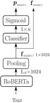
(a) BERTC

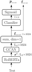
(b) GCAN

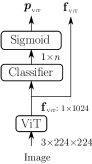
(c) ViT

Figure 1: Uni-modal models, where $\textrm{L}_{S}$ is the sequence length, which depends on the RoBERTa tokenizer.

Figure 1 depicts the three uni-modal models BERTC (1(a)), GCAN (1(b)), and ViT (1(c)), which form the basis of our further experiments. The bi-modal models are constructed based on trained uni-modal models and our proposed model fusion network, which is further detailed in Section 3.2. Finally, we apply soft and hard voting ensembles on the trained candidate models.

3.1 Uni-modal models

As illustrated in Figure 1, every uni-modal model has two outputs: the classification probabilities $\textbf{{p}}_{\textrm{{i}}}$ and the classification features $\textrm{{f}}_{\textrm{{i}}}$. All classifier blocks in our models have the following, identical structure: a fully connected layer reduces the feature dimension to half the input dimension, followed by a ReLU activation and a dropout layer. Ultimately, an output layer projects the features to the output dimension $n$, and a sigmoid function squashes the range of the output vector components to $(0,1)$, allowing for an interpretation as a vector of label probabilities, with possible overlap in categories.

BERTC: We fine-tune a pre-trained large RoBERTa language model (roberta-large) for classification. The text input is encoded by the RoBERTa model with the embedding dimension 1024. The Pooler layer returns the first classification token [cls] embedding $\textrm{{f}}_{\textrm{{BERTC}}}$ and feeds it into the classifier to obtain the probabilities $\textbf{{p}}_{\textrm{{BERTC}}}$.

GCAN: Again, a pre-trained RoBERTa model extracts contextual text information. Each token is considered as a word node and each meme is a document node. Thus the word node representation is given by the corresponding RoBERTa word embedding vector. We denote the input embedding sequence of document $k$ as $\textbf{{x}}^{k}=[\textbf{{x}}_{1}^{k},\textbf{{x}}_{2}^{k},\cdots\textbf{{x}}_{\textrm{L}_{S}}^{k}]$, where $\textbf{{x}}_{i}^{k}$, $i\in\{1,\ldots,\textrm{L}_{S}\}$ is a 1024-dimensional embedding vector of the $i$-th token. As depicted in Figure 1(b), $\textbf{{x}}^{k}$ is an $\textrm{L}_{S}\times$1024 matrix. The first classification token [cls] embedding represents the document classification information. Thus, we use the document-word co-occurrence information TF-IDF as the edge weights for the [cls] embedding. All other token embeddings are weighted with the word co-occurrence information PMI.

For each document $k$, we extract its specific adjacency matrix ${\stackrel{{\scriptstyle\sim}}{{\smash{\textbf{{A}}}\rule{0.0pt}{4.73611pt}}}}_{k}$ from the complete adjacency matrix ${\stackrel{{\scriptstyle\sim}}{{\smash{\textbf{{A}}}\rule{0.0pt}{4.73611pt}}}}$ by reducing it to rows and columns of all the document and word nodes ($i$ and $j$ in Equation 2) that are present in this document. The extracted document adjacency matrix ${\stackrel{{\scriptstyle\sim}}{{\smash{\textbf{{A}}}\rule{0.0pt}{4.73611pt}}}}_{k}$ is an $\textrm{L}_{S}\times\textrm{L}_{S}$ matrix.

The GCAN block in Figure 1(b) adopts the multi-head self-attention mechanism in 3 successive GCAN layers to embed the node representations. The queries Q, keys K and values V are identical and set to the respective layer input. The first layer input is given by the RoBERTa word embeddings $\textbf{{x}}^{k}$ of the input text. The attention of head $j$ is obtained by

$$\bm{\alpha}_{j}=\textrm{softmax}\left(\frac{\left(\textbf{W}_{j}^{Q}\textbf{Q}^{T}\right)^{T}\left(\textbf{W}_{j}^{K}\textbf{K}^{T}\right)}{\sqrt{d_{k}}}\right)\left(\textbf{W}_{j}^{V}\textbf{V}^{T}\right)^{T}$$ (3)

where $\textbf{W}_{j}^{\ast}$ are learned parameters for the queries Q, keys K, and values V, respectively. A superscript $T$ denotes the transpose; $d_{k}=\frac{d_{att}}{h}$, $d_{att}$ is the attention dimension and $h$ is the number of attention heads. Having computed the multi-head self-attention, each attention head output is multiplied by the document adjacency matrix ${\stackrel{{\scriptstyle\sim}}{{\smash{\textbf{{A}}}\rule{0.0pt}{4.73611pt}}}}_{k}$

$$\overset{\sim}{\bm{{\alpha}}}_{j}={\stackrel{{\scriptstyle\sim}}{{\smash{\textbf{{A}}}\rule{0.0pt}{4.73611pt}}}}_{k}\bm{\alpha}_{j}.$$ (4)

Equation 5 describes the output $\bm{\alpha}$ of the GCAN layer: The weighted outcomes all heads are concatenated (concat), and a fully connected layer (FC) projects the representation to the attention dimension. Inspired by Veličković et al. (2017), instead of concatenating the weighted attention head outputs, we employ averaging (avg) to fuse these weighted outputs in the last GCAN layer. A fully connected layer again projects the final representation to the attention dimension. Thus, after the GCAN block, the text representation is still an $\textrm{L}_{S}\times$1024 matrix. The document classification feature vector $\textrm{{f}}_{\textrm{{GCAN}}}$ is obtained by summing all node representations.

$$\bm{\alpha}=\left\{\begin{matrix}\textrm{FC}\left(\textrm{concat}\left(\overset{\sim}{\bm{{\alpha}}}_{1},\cdots\overset{\sim}{\bm{{\alpha}}}_{h}\right)\right)&\textrm{not in last layer}\\ \textrm{FC}\left(\textrm{avg}\left(\overset{\sim}{\bm{{\alpha}}}_{1},\cdots\overset{\sim}{\bm{{\alpha}}}_{h}\right)\right)&\textrm{in last layer}\\ \end{matrix}\right.$$ (5)

ViT: To extract the visual contextual information, we utilize the pre-trained ViT model vit-large-patch16-224 to encode the input image. For this purpose, the input image is split into fixed-size patches, and a linear projection of the flattened patches is used to obtain the patch embedding vectors. The Transformer encoder transforms the embedding vectors. Finally, the embedding $\textrm{{f}}_{\textrm{{ViT}}}$ of the first classification token, [cls], is fed to the classifier to obtain the prediction probabilities $\textbf{{p}}_{\textrm{{ViT}}}$.

3.2 Bi-modal models

Figure 2 shows our fusion model structure.

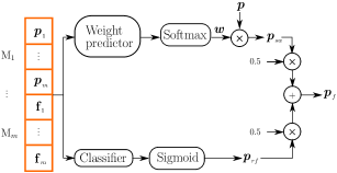
Figure 2: Fusion model structure

Each model $\textrm{M}_{i}$ has two outputs: the vector of its classification probabilities $\textbf{{p}}_{i}$ and the classification features $\textrm{{f}}_{i}$. We concatenate the model classification probabilities and features as a multi-modal representation to make the final decision.

Two fusion strategies—stream-weighting-based decision fusion and representation fusion—are considered. The weight predictor and the classifier in Figure 2 both have the same structure as the classifier block in Figure 1. The weight predictor output dimension is the number $m$ of candidate models for fusion. The stream weighting probability $\textbf{{p}}_{sw}$ is obtained through a weighted combination of the class probability vectors of all uni-modal model outcome probabilities, i.e.

$$\textbf{{p}}_{sw}=\sum_{i}\textbf{{p}}_{i}\cdot w_{i}.$$ (6)

The classifier output dimension is the same as the number of classes $n$. A sigmoid function computes the representation fusion probabilities $\textbf{{p}}_{rf}$ from the combined multi-modal representation. Finally, we average the stream weighting and the representation fusion probabilities. The following model combinations are attempted, where $\textrm{M}_{i}$, $i\in{\{1,2,3\}}$ is the $i$-th pre-trained uni-modal model.

Bi-modal model	$\textrm{M}_{1}$	$\textrm{M}_{2}$	$\textrm{M}_{3}$
BERTC-ViT	BERTC	ViT	-
GCAN-ViT	GCAN	ViT	-
BERTC-GCAN	BERTC	GCAN	-
BERTC-GCAN-ViT	BERTC	GCAN	ViT

3.3 Ensemble learning

Having established a number of possible uni-modal and bi-modal models, we now combine these trained models into ensembles. It has been reported in many studies that ensemble learning can enhance performance in comparison to single learners Onan et al. (2016); Zhu (2020); Gomes et al. (2017). Therefore, we consider soft and hard voting ensemble approaches.

We use the Python sklearn package for 10-fold cross-validation. Thus, each model structure was trained ten times with different inner test sets. Finally, these ten models are used to evaluate the official test set and deliver ten predictions for every sample. The soft voting ensemble method is implemented as follows: $\textbf{{p}}_{\textrm{M}_{i}}$, the ensemble probabilities that are used in the overall class decisions, are computed via

$$\textbf{{p}}_{\textrm{M}_{i}}=\sum_{j=0}^{9}w_{\textrm{M}_{i}}^{j}\cdot\textbf{{p}}_{\textrm{M}_{i}}^{j}.$$ (7)

Here, $\textbf{{p}}_{\textrm{M}_{i}}^{j}$ denotes the probabilities of model $\textrm{M}_{i}$ in the $j$-th fold. The weights $w_{\textrm{M}_{i}}^{j}$ are computed by

$$w_{\textrm{M}_{i}}^{j}=\frac{\textrm{F1}_{\textrm{M}_{i}}^{j}}{\sum_{f}\textrm{F1}_{\textrm{M}_{i}}^{f}}.$$ (8)

$\textrm{F1}_{\textrm{M}_{i}}^{j}$ corresponds with the best F1-score of model $\textrm{M}_{i}$ over all epochs, computed on the inner test set in fold $j$. This soft voting ensemble, using the same model structure, but with the multiple outcomes from 10-fold cross-validation, is referred to as a dataset-level ensemble in the following.

The second type of ensemble—the model-level ensemble—is constructed from the dataset-level ensemble results of each model. We use a hard voting strategy with seven candidate models (BERTC, GCAN, ViT, BERTC-ViT, GCAN-ViT, BERTC-GCAN, and BERTC-GCAN-ViT). In this approach, we set the final prediction for a data point to one, if at least half of the considered models vote one, making it a simple majority-voting strategy.

4 Experimental Setup

In this section, we describe our data processing and training pipeline in more detail.

4.1 Data pre-processing

The challenge dataset provides a transcription text stream that was obtained via OCR. Via image captioning, we derive a second text stream that contains a description of the image in a few words.

For the OCR text, we first use the Python ftfy package to fix the garbled sequences that result from unexpected encodings (the mojibake) like "පටà·". Next, all "@", "#" symbols and website addresses are removed from the text. The emojis are converted to text form by the Python emoji package. Finally, we remove non-English characters and convert the text to lowercase.

For image captioning, we utilize a pre-trained encoder-decoder attention model Xu et al. (2016). Although the translation from image to text is not very accurate, most likely owing to issues like the overlaid meme text, it was nonetheless beneficial for our classification task. We found that the description becomes more precise, when we split the memes into their constituent sub-images where applicable. In that case, the image caption is extracted over every sub-image as well as the entire meme. Finally, the image captions are combined with the word "and" and then concatenated with the OCR text, separated by ". ". With this rule, the final text of the meme in Figure 3 is: "mgo ci aindo make make me sandwich!!. a couple of baseball players standing next to each other and a woman holding a sign in front of a sign and a woman standing next to a group of people."

(a) a woman holding a sign in front of a sign

(b) a couple of baseball players standing next to each other

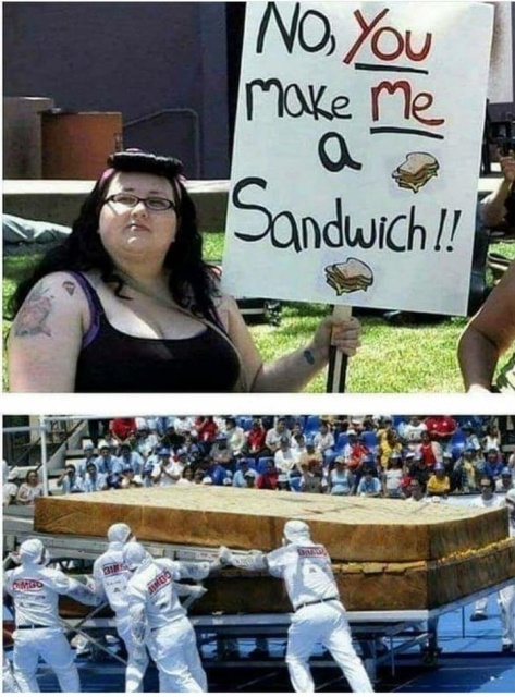
(c) a woman standing next to a group of people

Figure 3: In (a) and (b), we see "sub-images" and corresponding captions. (c) shows the meme and its caption (when not considering the sub-image structure).

We use the entire meme as the image input for ViT. All memes are first resized to 256$\times$256 and center-cropped to 224$\times$224 dimensions. The ViT model uses all 3 RGB channels, so we retain the RGB structure, thus the input image dimension is 3$\times$224$\times$224. We regularize the entire image database to range 0 to 1, then normalize each individual image to have zero mean and unit variance.

4.2 Loss function

We decided to use the binary cross-entropy (BCE) loss for both subtasks.

Due to the imbalance in the class distributions (see Table 1), in sub-task B, we weighted the class-specific loss terms by their support as follows:

$$w_{c}=\frac{\frac{\textrm{NoS}}{\textrm{NoS}(c)}}{\sum_{c^{\prime}}\frac{\textrm{NoS}}{\textrm{NoS}(c^{\prime})}},c\in[\textrm{Shm},\textrm{Ste},\textrm{Obj},\textrm{Vio}]$$ (9)

where NoS is the total number of samples in the training set and $\textrm{NoS}(c)$ represents the number of true instances for class $c$. The loss is then computed through the weighted combination of the single BCE terms:

$$\mathcal{L}_{1}=\sum_{c}w_{c}\cdot\textrm{BCE}(\textbf{{p}}_{c}^{B},\textbf{{y}}_{c}^{B}).$$ (10)

Here, $\textbf{{p}}_{c}^{B}$ represents the system’s output probability of class $c$ and $\textbf{{y}}_{c}^{B}$ is the binary ground truth for sub-task B.

Additionally, we employ a teacher forcing loss to connect both subtasks. The idea is that an instance should be identified as misogynous and possibly grouped into sub-categories simultaneously. The teacher forcing loss is defined as:

$$\mathcal{L}_{2}=\lVert\textbf{{p}}^{A}-\textbf{{y}}^{A}\rVert,$$ (11)

where the system’s output probability for sub-task A is determined as:

$$\textbf{{p}}^{A}=\textrm{max}\big{(}\textbf{{p}}_{{}_{\textrm{Shm}}}^{B},\textbf{{p}}_{{}_{\textrm{Ste}}}^{B},\textbf{{p}}_{{}_{\textrm{Obj}}}^{B},\textbf{{p}}_{{}_{\textrm{Vio}}}^{B}\big{)}.$$ (12)

The final loss is computed by

$$\mathcal{L}=0.7\cdot\mathcal{L}_{1}+0.3\cdot\mathcal{L}_{2}.$$ (13)

4.3 Model training

All models are trained using the PyTorch library Paszke et al. (2019) for 50 epochs. The AdamW optimizer Loshchilov and Hutter (2017) is used for backpropagation, using a linear learning rate scheduler with a warm-up to adapt the learning rate during the first four epochs in the training stage. The dropout rate is 0.5. The RoBERTa model parameters in the BERTC and the GCAN model are optimized separately.

In our GCAN model, the adjacency matrix is computed with a sliding window of length 10. An 8-head self-attention is applied over 3 GCAN layers with an attention dimension of 1024.

For all uni-modal models, the batch size is 16 and the initial learning rate is $2\cdot 10^{-5}$. The RoBERTa and ViT block parameters in Figure 1 are also fine-tuned. The bi-modal models are trained based on the pre-trained uni-modal models. Here, we choose the batch size as 32, the initial learning rate is $5\cdot 10^{-6}$. As the RoBERTa and ViT block parameters in Figure 1 are already updated during the uni-modal training stage, we froze these parameters in bi-modal re-training.

To avoid overfitting, we adopt early stopping to exit the training process when the computed F1-score on the inner test set does not increase over 4 epochs. Inspired by Huang et al. (2017), we finally averaged those two epoch-wise model parameters, which had the highest validation F1-score during the training stage.

The models have the same structure for sub-tasks A and B. The only differences are that in sub-task A, the classifier output dimension $n$ is $1$, and the BCE is used as the loss function (Setup A), whereas in sub-task B, the classifier output dimension $n$ equals $4$ and training uses the weighted BCE with teacher forcing (Equation 13) as the loss function (Setup B). All models are trained using NVIDIA’s Volta-based DGX-1 multi-GPU system, using 3 Tesla V100 GPUs with 32 GB memory each.

5 Results

In summary, we investigated two configurations, displayed in Table 2. Setup A represents the binary classification for sub-task A, resulting in an output dimension $n=1$. Setup B additionally deals with the multi-label classification of sub-task B, returning an output of dimension $n=4$. All results are evaluated on the official test set.

Setup	Task	Dimension	Loss
Setup A	sub-task A	$n=1$	BCE
Setup B	sub-tasks A/B	$n=4$	Weighted BCE & Teacher Forcing

Table 2: Summary of the considered configurations.

5.1 Results for Setup A (Sub-task A)

In the first stage, we trained three different uni-modal models (i.e., BERTC, GCAN, and ViT). In the second stage, we optimized the bi-modal models (i.e., BERTC-ViT, GCAN-ViT, BERTC-GCAN, and BERTC-GCAN-ViT). The evaluation results in terms of the macro-average F1-score are displayed in Figure 4 and Table 3, showing the performance in identifying misogynous memes. To assess the statistical significance of performance differences, we applied a 10-fold cross validation and computed the Mann-Whitney-U test Mann and Whitney (1947).

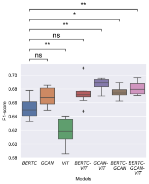
Figure 4: Macro-average F1-scores for sub-task A based on 10-fold cross validation. Asterisks indicate a statistically significant difference, where ** denotes 1e-04 < p <= 1e-03, * corresponds to 1e-02 < p <= 5e-02, and ns indicates results where p > 5e-02.

As we can see, the text-only models (BERTC and GCAN) generally show a superior performance compared to the image-only model (ViT). The results in Figure 4 clearly indicate robust performance for our bi-modal models. They are more accurate and robust. In summary, the GCAN-ViT model yields the best results w.r.t. the reported median F1-score.

Model	Ensemble	Model	Ensemble
BERTC	0.663	GCAN-ViT	0.707
GCAN	0.674	BERTC-GCAN	0.677
ViT	0.619	BERTC- GCAN-ViT	0.689
BERTC-ViT	0.697	-	-

Table 3: Macro-average F1-scores of soft voting ensembles for sub-task A.

Table 3 lists the averaged F1-scores for soft voting ensembles, obtained by combining all learned models from the 10-fold cross-validations. The results show that our GCAN-ViT model outperforms all other models, achieving an F1-score of 0.707.

5.2 Results for Setup B (Sub-tasks A/B)

Next, we addressed sub-task B, i.e. to classify the misogynous memes into four, potentially overlapping, categories. Similar to Setup A, we trained the same uni- and bi-modal models, but incorporating a different loss (see Table 2). For sub-task B, the weighted-average F1-score is applied. The results are presented in Figure 5.

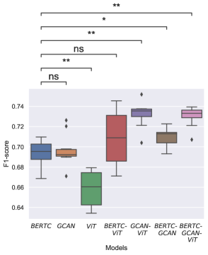
(a) Results for sub-task A.

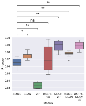
(b) Results for sub-task B.

Figure 5: Performance for Setup B. The notation is defined in Figure 4.

Interestingly, the models optimized for sub-task B also perform better for sub-task A. In this case, we set the estimated label "misogynous" to 1 if at least one of the labels for "shaming", "stereotype", "objectification", or "violence" is 1.

Figure 5(a) depicts the sub-task A results while Figure 5(b) shows the corresponding performance for sub-task B. Again, we see that the bi-modal model GCAN-ViT outperforms all other models.

In addition, Tables 4 and 5 show the results for soft and hard voting ensembles. By comparing Table 4 with Table 3 (both tables represent soft voting results), we observe significantly improved F1-scores for Setup B.

Model	Sub-task A	Sub-task B
BERTC	0.714	0.684
GCAN	0.725	0.695
ViT	0.666	0.641
BERTC-ViT	0.746	0.692
GCAN-ViT	0.758	0.704
BERTC-GCAN	0.724	0.696
BERTC-GCAN-ViT	0.755	0.704

Table 4: F1-scores of soft voting ensembles for Setup B (sub-tasks A and B).

Combination	Sub-task A	Sub-task B
Three uni-modal models	0.728	0.698
Four bi-modal models	0.752	0.709
All seven models	0.755	0.706
Oracle model combination	0.762	0.716

Table 5: Model-level hard voting ensemble performance with Setup B for sub-task A and B.

As a last experiment, we applied hard voting on the ensembles. Again, sub-task A results are derived from sub-task B.

Table 5 shows the results of different combinations. Generally, the combination of the four bi-modal models in the 2nd row outperforms a combination of three uni-modal models in the 1st row. If we combine all uni- and bi-modal models (3rd row), the F1-score is 0.755 for sub-task A, and 0.706 for sub-task B.

The results in bold print represent our submitted approaches for both sub-tasks, showing an F1-score of 0.755 for sub-task A and 0.709 for sub-task B.

After the challenge ended, we again evaluated all possible subset combinations of the seven candidate models. The followed combinations give the best achievable results by knowing the official test set reference labels: ViT, BERTC-GCAN-ViT, BERTC-ViT, GCAN-ViT achieves an F1-score of 0.762 for sub-task A, while an ensemble consisting of BERTC-ViT and BERTC-GCAN-ViT yields an F1-score 0.716 on sub-task B. These results are shown for comparison in the final row of Table 5 as oracle results.

6 Conclusion

This paper presents our ensemble-based approach to address two sub-tasks of the SemEval-2022 MAMI competition. The challenge aims to identify misogynous memes and classify them into—potentially overlapping—categories. We train different text models, an image model, and via our proposed fusion network, we combine these in a number of different bi-modal models.

Among the uni-modal systems, all text models show a far better performance than the image model. As expected, our proposed graph convolutional attention network (GCAN), which also considers the graph structure of the input data while using pre-trained RoBERTa word embeddings as node features, consistently outperforms the pre-trained RoBERTa model.

The proposed fusion network further improves the performance by combining the ideas of stream-weighting and representation fusion. We additionally adopt 10-fold cross-validation and use a dataset-level soft voting ensemble to obtain better and more robust results. Finally, our model-level hard voting ensemble integrates the soft voting ensemble predictions of our best uni- and bi-modal models. Our experiments indicate that this layered ensemble approach can significantly improve the model accuracy. Ultimately, our submitted system results in an F1-score of 0.755 for sub-task A and 0.709 for sub-task B.

Overall, we believe that the identification of misogyny in memes is best addressed through bi-modal recognition, considering both textual and image information. Concerning the text-based classification, we found a graph convolutional attention neural network to be beneficial as an integrative model for Transformer embeddings. This helps in the text classification, when the documents are short, as for the given meme classification task.

To cope with the bi-modality of the task at hand, we have implemented a range of systems for integrating the information from both streams. An idea that proved to be effective here was that of bringing together the strengths of early fusion and decision fusion in a joint framework. This allowed us to dynamically adjust the contributions of the two modalities through dynamic stream weighting, while still being able to combine information at the feature level across the streams, thanks to the representation fusion branch of our bi-modal systems.

References

- Chetty and Alathur (2018) Naganna Chetty and Sreejith Alathur. 2018. Hate speech review in the context of online social networks. Aggression and violent behavior, 40:108–118.
- Dosovitskiy et al. (2020) Alexey Dosovitskiy, Lucas Beyer, Alexander Kolesnikov, Dirk Weissenborn, Xiaohua Zhai, Thomas Unterthiner, Mostafa Dehghani, Matthias Minderer, Georg Heigold, Sylvain Gelly, et al. 2020. An image is worth 16x16 words: Transformers for image recognition at scale. arXiv preprint arXiv:2010.11929.
- Fersini et al. (2022) Elisabetta Fersini, Francesca Gasparini, Giulia Rizzi, Aurora Saibene, Berta Chulvi, Paolo Rosso, Alyssa Lees, and Jeffrey Sorensen. 2022. SemEval-2022 Task 5: Multimedia automatic misogyny identification. In Proceedings of the 16th International Workshop on Semantic Evaluation (SemEval-2022). Association for Computational Linguistics.
- Gomes et al. (2017) Heitor Murilo Gomes, Jean Paul Barddal, Fabrício Enembreck, and Albert Bifet. 2017. A survey on ensemble learning for data stream classification. ACM Computing Surveys (CSUR), 50(2):1–36.
- Huang et al. (2017) Gao Huang, Yixuan Li, Geoff Pleiss, Zhuang Liu, John E. Hopcroft, and Kilian Q. Weinberger. 2017. Snapshot ensembles: Train 1, get M for free. In 5th International Conference on Learning Representations, ICLR 2017, Toulon, France, April 24-26, 2017, Conference Track Proceedings.
- Kiela et al. (2020) Douwe Kiela, Hamed Firooz, Aravind Mohan, Vedanuj Goswami, Amanpreet Singh, Pratik Ringshia, and Davide Testuggine. 2020. The hateful memes challenge: Detecting hate speech in multimodal memes. Advances in Neural Information Processing Systems, 33:2611–2624.
- Liu et al. (2019) Yinhan Liu, Myle Ott, Naman Goyal, Jingfei Du, Mandar Joshi, Danqi Chen, Omer Levy, Mike Lewis, Luke Zettlemoyer, and Veselin Stoyanov. 2019. Roberta: A robustly optimized bert pretraining approach. arXiv preprint arXiv:1907.11692.
- Loshchilov and Hutter (2017) I. Loshchilov and F. Hutter. 2017. Decoupled weight decay regularization. arXiv preprint arXiv:1711.05101.
- Lu et al. (2020) Zhibin Lu, Pan Du, and Jian-Yun Nie. 2020. VGCN-BERT: augmenting BERT with graph embedding for text classification. Advances in Information Retrieval, 12035:369.
- Mann and Whitney (1947) H. Mann and D. Whitney. 1947. On a test of whether one of two random variables is stochastically larger than the other. The annals of mathematical statistics, pages 50–60.
- Onan et al. (2016) Aytuğ Onan, Serdar Korukoğlu, and Hasan Bulut. 2016. Ensemble of keyword extraction methods and classifiers in text classification. Expert Systems with Applications, 57:232–247.
- Paszke et al. (2019) A. Paszke, S. Gross, F. Massa, A. Lerer, J. Bradbury, G. Chanan, T. Killeen, Z. Lin, N. Gimelshein, L. Antiga, et al. 2019. Pytorch: An imperative style, high-performance deep learning library. Advances in neural information processing systems.
- Sabat et al. (2019) Benet Oriol Sabat, Cristian Canton Ferrer, and Xavier Giro-i Nieto. 2019. Hate speech in pixels: Detection of offensive memes towards automatic moderation. arXiv preprint arXiv:1910.02334.
- Simonyan and Zisserman (2014) Karen Simonyan and Andrew Zisserman. 2014. Very deep convolutional networks for large-scale image recognition. arXiv preprint arXiv:1409.1556.
- Torrey and Shavlik (2010) Lisa Torrey and Jude Shavlik. 2010. Transfer learning. In Handbook of research on machine learning applications and trends: algorithms, methods, and techniques, pages 242–264. IGI global.
- Vaswani et al. (2017) Ashish Vaswani, Noam Shazeer, Niki Parmar, Jakob Uszkoreit, Llion Jones, Aidan N Gomez, Łukasz Kaiser, and Illia Polosukhin. 2017. Attention is all you need. In Advances in neural information processing systems, pages 5998–6008.
- Veličković et al. (2017) Petar Veličković, Guillem Cucurull, Arantxa Casanova, Adriana Romero, Pietro Lio, and Yoshua Bengio. 2017. Graph attention networks. arXiv preprint arXiv:1710.10903.
- Wang et al. (2020) Ling Wang, Chengyun Zhang, Renren Bai, Jianjun Li, and Hongliang Duan. 2020. Heck reaction prediction using a transformer model based on a transfer learning strategy. Chemical Communications, 56(65):9368–9371.
- Xu et al. (2016) Kelvin Xu, Jimmy Ba, Ryan Kiros, Kyunghyun Cho, Aaron Courville, Ruslan Salakhutdinov, Richard Zemel, and Yoshua Bengio. 2016. Show, attend and tell: Neural image caption generation with visual attention.
- Yao et al. (2019) Liang Yao, Chengsheng Mao, and Yuan Luo. 2019. Graph convolutional networks for text classification. In Proceedings of the AAAI conference on artificial intelligence, 01, pages 7370–7377.
- Zhu (2020) Ron Zhu. 2020. Enhance multimodal transformer with external label and in-domain pretrain: Hateful meme challenge winning solution. arXiv preprint arXiv:2012.08290.