Minimum Distance and Parameter Ranges of Locally Recoverable Codes with Availability from Fiber Products of Curves
Abstract
We construct families of locally recoverable codes with availability using fiber products of curves, determine the exact minimum distance of many families, and prove a general theorem for minimum distance of such codes. The paper concludes with an exploration of parameters of codes from these families and the fiber product construction more generally. We show that fiber product codes can achieve arbitrarily large rate and arbitrarily small relative defect, and compare to known bounds and important constructions from the literature.
1 Introduction
A code is broadly said to be locally recoverable if an erased symbol in any position in a codeword of can be recovered by consulting a small number of symbols in other (fixed) positions, called a recovery set for position . Locally recoverable codes have been widely studied in recent years for their potential applications in reliable and efficient cloud storage. For a survey on this topic, see [1].
A natural next property to look for in locally recoverable codes is the ability to recover more than one erasure. There are two main approaches to this question. First, one could ask that the single recovery set for each position allow for recovery of additional erasures within the set, introducing the parameter to recover erasures. Alternatively, one could ask that each position has multiple (usually disjoint) recovery sets, introducing the parameter to represent the number of recovery sets that each position has. Of course, these two approaches can also be blended, producing multiple recovery sets that each can recover multiple erasures. While this work focuses on the second approach for simplicity, the main construction can be adapted to blend with the first approach.
The Tamo-Barg method [10, 11] of constructing locally recoverable codes is based on building a particular linear space of functions on an evaluation set . The set is partitioned into extended recovery sets based on algebraic or geometric relationships between the points in , and functions in are chosen so that they restrict to polynomials of a single variable of bounded degree on each extended recovery set. If the value of the function at any point in an extended recovery set is erased, it can be recovered through single variable polynomial interpolation using the values of the function on the other points in the set. There is a large body of work building on this approach. In [2], the authors construct locally recoverable codes with availability based on fiber products of curves and propose a group-theoretic perspective on the construction. In [5], the authors generalize the fiber product construction to and refine the parameters of the resulting codes. The group-theoretic method of constructing locally recoverable codes with many recovery sets has also been studied, notably in [3]. The general approach of creating locally recoverable codes from rational maps is pursued in [7] and extended to algebraic curves defined by equations with separated variables in [8], but the general fiber product construction still requires more exploration.
This work is an extension of [5], with a goal of understanding the range of possibilities and limitations of this construction. For completeness, we include the relevant definitions and construction from [5]. In Section 2, we include some expository discussion on ways to think of the fiber product of curves and special cases of the construction. We then introduce the three families of codes which are the main examples of this paper. These three families are all centered on the well-studied Hermitian curve . The first main example family, introduced in Example 3.1 comes from the Hermitian curve, introduced as an example of a locally recoverable code with two recovery sets in [2]. The second, Example 3.2 is a novel code based on the fiber product of two Hermitian curves, and is designed to illustrate the flexibility of this method–one can select curves with appropriate maps and understand the fiber product, and therefore the parameters of the code, using geometry and the construction of [5]. The final example, Example 3.3, is a code from a fiber product of Artin-Schreier curves introduced by van der Geer and van der Vlugt. This example was introduced in [5] and is included as an example where can be as large as desired. When the construction is defined over , for a prime and a natural number, and we choose factor curves, the fiber product is again the Hermitian curve .
In Section 4, we calculate the exact minimum distance for the first family and for a large range of examples in the third family in Theorems 4.1 and 4.3. Incidentally, we also compute the exact minimum distance of a non-fiber product code introduced in [2] in Theorem 4.2. This is followed by Theorem 4.4 on minimum distance for codes defined using a fiber product. We apply Theorem 4.4 to particular examples in the second and third family in Examples 4.2 and 4.1.
Finally, in Section 5, we explore the parameter space and compare to some relevant bounds and constructions from the literature. We show in Corollary 5.1 that fiber product codes are not able to surpass the rate of the product code construction from [10], though some constructions are extremely close.
Acknowledgments
The authors would like to thank the organizers and participants in the Rethinking Number Theory workshop for creating a lauch pad for part of our research group, and helping us build an inclusive research environment that accommodated all researchers’ workloads and backgrounds. We particularly thank early group members Ernest Guico, Darleen Perez-Lavin, and Alexader Diaz-Lopez for their valuable contributions to our understanding. Author Kottler was supported by the Summer Collaborative Research Experience award from Colorado College. This material is based upon work supported by the National Science Foundation under Grant No. 2137661.
2 Preliminaries
2.1 Locally Recoverable Codes and Availability
Let be natural numbers, with . A linear code of length and dimension over the field is a -dimensional linear subspace of . The minimum distance of is the minimum number, , of coordinates in which two distinct elements of (referred to as codewords) must differ. The weight of a codeword is the number of non-zero coordinates it has, for the codeword , we denote this value by . As a vector space, the minimum distance of is equal to the minimum weight of the non-zero codewords. It is common to refer to such codes as -codes.
For an -code, the rate of the code is . The relative minimum distance is given by . When a Singleton-type upper bound on minimum distance is known, we define the defect of the code to be and the relative defect of the code to be .
We say is a locally recoverable code (LRC) with locality if for all there exists a set of indices and a function such that and for all codewords we have . The set is called the recovery set for the -th position. It may be desirable to have multiple disjoint recovery sets for each position to protect against multiple erasures or allow for simultaneous queries of heavily-accessed information. A locally recoverable code has availability with locality if for each there exists sets of indices such that
-
1.
for
-
2.
-
3.
For each there exists a function such that for all codewords we have .
We refer to an LRC with availability as an LRC(). The localities of an LRC() form a vector . When for all , we say that the code has uniform locality .
2.2 Evaluation Codes on Curves
Let be an algebraic variety defined over a finite field . Let be a subset of of cardinality , with points arbitrarily ordered as . Let be a linear subspace of the function field such that no function in has poles at any point in . For any , define the evaluation map
Then we define the evaluation code as
Reed-Solomon codes are evaluation codes where is the space of polynomials of bounded degree and are the values in a finite field, viewed as affine points on a projective line. Evaluation codes on the Hermitian curve have also been very well-studied. For any prime power , the Hermitian curve is defined over any extension of by the affine equation
The curve has genus and has points over including a single point at infinity.
2.3 Fiber Products of Curves
Let , , and be projective curves over , with maps that are separable, rational -morphisms for . The fiber product is a curve that is (abstractly) defined using the corresponding fiber product of schemes. More concretely, the -rational points of the fiber product are given by
The fiber product construction can be iterated and is seen to be (up to isomorphism) associative and commutative. Thus for any , we may without confusion construct the -fold fiber product of curves as follows. Let be projective curves over with separable -rational maps . The -points of the fiber product of over are then given by
A simple visualization of a 2-fold fiber product construction is given in Figure 2.1.
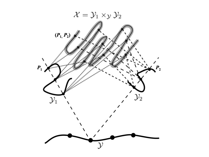
This construction induces natural projection maps
from the fiber product onto each factor curve. Let
be the fiber product of all curves except . Then we see that is isomorphic to , and we identify with the isomorphic factor in the original fiber product construction of . This gives complementary projection maps
We also define the map by for any .
Remark 2.1.
Simply speaking, the map “forgets” the information coming from the curve while retaining the data of the fiber product that come from the other curves.
The function field is isomorphic to the compositum of the function fields , where the function field is embedded into each as induced by the map . For ease of exposition, we identify each function field with its image inside , so for each . Further, we assume that is the full field of constants within each of these fields, and that
| (2.1) |
Remark 2.2.
If 2.1 holds and either each extension is Galois, or the degrees are pair-wise relatively prime, then these extensions are linearly disjoint and the degree of is the product of the degrees , i.e. . In this case, we have .
2.4 Locally Recoverable Code with Availability Construction from Fiber Product
The following general construction comes from [5], though for completeness we include it simplified notation here. Let so that . For each , , we choose so that , where is the root of an irreducible separable polynomial . Let be the degree of the function .
We now have that
The degree of must be equal to the degree of , denoted .
Now, choose such that
-
•
for all (i.e. all places in split completely in the extension ) and
-
•
for each , , the function has no poles at any point above in the extension .
Choose an effective divisor of degree on with , so functions in the Riemann-Roch space have no poles in . Let be a basis of the Riemann-Roch space . We require that so that for all , there exists some with . Let be the -vector space with basis
| (2.2) |
Then set
| (2.3) |
where an arbitrary ordering of elements is fixed on . Note that .
The code is locally recoverable with availability . Recall that we have fixed an ordering of the points in for the evaluation map . For any with and , set
Let
Consider a codeword for some function . Given an erasure in position of the codeword (associated with point ), each acts as a recovery set, because on the set the function is constant except in , so on it acts as , a polynomial of degree less than or equal to . The evaluation of on the points of therefore give rise to distinct pairs . Since any polynomial of this degree is determined by its values on points, these pairs are sufficient to determine the value of .
This construction gives rise to the following theorem.
Theorem 2.1.
One may easily calculate the rate of the constructed code. In the case that the extensions are linearly disjoint, we have an especially simple form.
Corollary 2.2.
If the extensions are linearly disjoint, then the rate of is
| (2.4) |
This is a simple application of the definition of rate, the fact that , and the fact that when the extensions are linearly disjoint, we have .
3 Simplified Framework and Featured Constructions
To gain some intuition, let us consider the simplest version of this fiber product construction: say with the unique point at infinity on this curve, and given by projection onto . In this case, the fiber product can be embedded into , with affine coordinates . Note that this fiber product, , is isomorphic to the intersection of hypersurfaces in -dimensional space. Further, if we take to be the divisor defining the Riemann-Roch space , then this fiber product construction results in a punctured subcode of the Reed-Muller code, with functions simply polynomials in and evaluation points a subset of points on the intersection of the -hypersurfaces created by considering the defining equations for the curves in . Explicitly, the functions leading to codewords are
General fiber product codes should be viewed as generalizations of these simple codes.
Let be an evaluation point of such a simple fiber product code, where . The -th recovery set for is the set of all evaluation points , where . That is, the -th recovery set is simply the set of all evaluation points which share all coordinate values but that of with .
We now introduce three important examples of fiber product codes within this simplified framework.
Example 3.1.
LRC(2)s on the Hermitian Curve Viewed as a Fiber Product As a first concrete example, we consider the Hermitian curve as a fiber product and intersection. Let , , and , and let be projection onto for . Then the fiber product is isomorphic to the curve . Indeed, the affine points of are given by
Hence this is isomorphic by the natural map to the intersection of the two hypersurfaces in with affine equations and , and also to the curve defined in by affine equation . The utility of the fiber product viewpoint on this curve is to highlight two natural maps which give rise to recovery sets. Codes using the fiber product construction of are developed in [2], where a lower bound is given on the minimum distance. Let be the LRC() presented in Proposition 5.1 of [2]. For this code, we take the curve with evaluation set We can check that . Then we let be the space of functions with basis The code is an LRC() where the two recovery sets for a point are given by the points , sharing the same -coordinate and those sharing the same -coordinate value as . These recovery sets are of size and , respectively.
In [2], the authors prove the following.
Theorem 3.1.
([2]) The code has length dimension and minimum distance
Applying the viewpoint of [5], we are able to tighten this bound.
Proposition 3.2.
The code has minimum distance satisfying
Proof.
First, we note that we may consider the Hermitian curve given as a fiber product as described above. Then is the set of all points of lying above points of that split completely in the extension . We obtain by letting be the zero divisor, so . Applying Theorem 2.1, we find that the minimum distance of is in fact bounded by
∎
In Theorem 4.1, we calculate exactly the minimum distance for this code.
Example 3.2.
LRC(2)s on the Fiber Product of two Hermitian Curves One can take the fiber product of any two curves with appropriate maps to the same base curve. As a simple example, we take a fiber product of two Hermitian curves. For a prime power, consider the Hermitian curves
From each of these there is a projection to via the coordinate, . Using these projections, we construct the fiber product .
Intuitively, the affine part of this fiber product is pairs of points on the Hermitian curve satisfying . Moreover
There is a single point at infinity for each Hermitian curve, so there is a single point at infinity for , which is totally ramified with ramification index in the extension .
Also, defining , we see that there are points of with -coordinate that are split completely in the extension (so have ramification index equal to ), and another points with -coordinate that ramify, but not completely; they have ramification index .
Since all ramification is tame in the extension , and , we can compute the arithmetic genus of the fiber product using Riemann-Hurwitz formula to get
Following the construction from [5], we now present a code with two recovery sets by the evaluation of the splitting points on . Let the set of points of that are above the points with -coordinate that split completely:
Let . Then the sets for are recovery sets for the position corresponding to . We have and .
We define
with .
Theorem 3.3.
For the fiber product with , and defined as above, the evaluation code is a locally recoverable -code over with availability and locality where
In Corollary 4.5, we calculate the minimum distance for this code.
Remark 3.1.
Here we give a concrete example of the preceding construction of . Let and , where , be the finite field with 9 elements. Let us consider the situation of Example 3.2, in which we have the fiber product of two Hermitian curves over :
along with the fiber product . In this case, , and we have 6 points on with first coordinate outside that split completely in . The maximum that can be chosen to get a non-trivial bound for is . Using this in Theorem 3.3, we get a LRC(2) of length , dimension and minimum distance over (an upper bound for the minimum distance is , see Section 5).
Example 3.3.
Artin–Schreier Fiber Product and LRC() In [5] the authors use a fiber product curve construction from van der Geer and van der Vlugt [13] to create codes with availability for arbitrary . Since we continue this example, we review the construction here.
The simplest of the van der Geer and van der Vlugt constructions is given in [13, Section 3, Method I]. Let be prime, a natural number, and . Let generate over . Then the curves
each have genus and have points over , with one point, , at infinity.
Let be an integer with and let . Then consider the natural map given by projection onto the coordinate, where represents the point at infinity on the projective line and . These are all degree- Artin–Schreier covers of , fully ramified above .
Define to be the fiber product of these curves over ; i.e.,
The corresponding maps are degree , ramified only above . Let be the single point above on .
As shown in [13, Theorem 3.1], the curve has genus and , making maximal over .
Note that the curve is naturally a subvariety of . It embeds in , however, by the map defined on affine points of via
From here, we identify with its image in . The affine points of are given by
| (3.1) |
For , the functions are given by
and the functions are given by
For each , the map has degree . For , the function has degree , since for each with and , there are points , where and .
Remark 3.2.
As observed in [5], when , we have that .
Applying the construction from [5], we can construct codes defined over with many recovery sets. Let . Then , the -th recovery set for the position corresponding to , is the set of positions corresponding to the points in We then have . On points corresponding to the positions in , any function in varies as a polynomial in of degree at most and can therefore be interpolated by knowing its values on any points.
Given as above, choose to ensure the evaluation map is injective. Note that the evaluation map may be injective for larger values of but that the given lower bound ensures that in the Theorem below. Let . Then is the set of polynomials in of degree at most , a vector space of dimension .
Theorem 3.4 ([5]).
Given the fiber product of the specified Artin–Schreier curves, with and as above, let , and as defined in Theorem 2.1. We define . Then is a locally recoverable -code over with availability and locality where
In Theorem 4.3, we compute the exact minimum distance of the code here for many values of .
4 Computing Minimum Distances
A standard technique for determining the minimum distance of an evaluation code is to first bound the minimum distance below using a geometric argument, then find an element in the space of functions that vanishes at the maximum number of points, all of which are contained in the evaluation set . Using the bounds from [5] and this technique, it is possible to find the exact minimum distance of some interesting codes from [2] and [5].
As a warm-up, we find the exact minimum distance of two LRCs on the Hermitian curve described in [2]. The first arises from a simpler rational map construction. Let be the code with locality described in Proposition 4.1 of [2], i.e., the evaluation code where is the Hermitian curve defined by , is the set of affine points in , and is the vector space of functions generated by for some fixed . Note that the recovery set for the position corresponding is the set of points
Theorem 4.1.
When , the code has minimum distance
Proof.
In [2], the authors prove that is a lower bound on the minimum distance of . Suppose . Considering the extension of fields to , let be the field trace map given by and let be the norm map given by . Since is the trace map, which is degree onto , we can write
Since is the norm map and so is degree onto , we can write
Define by
We see that has at most zeros. To show that has exactly that many zeros, we must show that no evaluation point of is sent to zero by more than one factor of . Suppose . Then , but by design hence Thus no evaluation point can be sent to zero by multiple factors, so has exactly zeros and has weight and the minimum distance is as given.
∎
Recall that is the LRC(2) on defined in [2]. We now determine the exact minimum distance of the code.
Theorem 4.2.
The code has minimum distance .
Proof.
Now let such that . Then let and . Because these come from the trace and norm respectively, we can write and . Then let be defined
The function has exactly zeros by the same argument as in the previous construction. Thus ∎
Next, we determine the exact minimum distance for many codes from the fiber product of Artin–Schreier curves constructed in Theorem 3.4.
Theorem 4.3.
Let be a prime and a prime power. For a fixed with , let be the LRC of Theorem 3.4, constructed using the fiber product of Artin–Schreier curves. Then has minimum distance
Proof.
Recall that the curves that we use to produce the fiber product are of the form
where . From Theorem 3.4, we have a lower bound for minimum distance, .
Let be defined by and be defined by the norm map . Choose values
and . Since is the norm map, , so . Thus we can write
By choice of , we have and since is a degree 2 extension, too. Then since we are working in characteristic and the trace map can be factored,
By the additive version of Hilbert’s Theorem 90, is nonempty. Notice that is separable of degree , so must, in fact, equal . We then write
Define the map by
Recall that , as in equation (3.1), is the evaluation set for polynomials in and is the length of . Certainly is at most . We wish to show that these values are equal by showing that has exactly this many zeros in by showing that no points in have component in and component in for all . Toward that end, suppose that such that .
Assume that for some . Then , so , by definition of . This equation has at most solutions, all of which are in the set . Since none of these are in , we have that .
Now suppose that for some we have . Then . Thus we have . Recall that is in the kernel of the trace map, so and so . Similarly . Substituting these values gives us the equality , so or , but and are elements of a basis for the kernel of over , so .
Thus has exactly zeros in , so the code has the desired minimum distance,
∎
4.1 A Condition for Exact Minimum Distance.
More generally, we may summarize the situation in which this technique will give the exact minimum distance of codes from the construction in Theorem 2.1.
Theorem 4.4.
Let be a locally recoverable code constructed as in Section 2.4, where has basis given by (2.2), is the evaluation set as in (2.3), and for . If it is possible to find sets such that
-
for all ,
-
,
-
for all ,
-
for all with there is no with -coordinate in and -coordinate in , and
-
for all with , the projection is not ramified over any point with
then the code has minimum distance
| (4.1) |
where is the length of the code.
Remark 4.1.
If , given by projection onto , and , as is the case in all examples in this paper, we have that for and is an unramified map above from the code construction.
Proof.
4.1.1 Examples of Applying Theorem 4.4
Here, we give two extremely concrete examples to illustrate the application of this general condition.
Example 4.1.
Let and , so and we work over . Let be a non-trivial fifth root of unity for which . Let and be generators of . Then we have explicit curves
Each of these curves has a projection onto via their -coordinate, which we will denote and . Consider their fiber product
which is a genus 36 curve. Each of the maps are degree 3 and ramified only above the point at infinity. We can realize the 729 affine points of to be the set
In order to satisfy the hypothesis of Theorem 4.4, it will suffice to find sets , , and with and , where . We choose and , each of which will eliminate possible values from entry into , as there are 10 points in with -coordinate and 10 with -coordinate . Thus values remain as possible elements of and hence we may use any value , to receive a code with the prescribed minimum distance, as in Theorem 4.4.
Example 4.2.
If we try to apply Theorem 4.4 to get the exact minimum distance for the code over constructed in Remark 3.1 we see that the sets , and cannot be built, so a minimum weight codeword cannot be constructed by this method and the miniumum distance cannot be determined by the theorem. Instead, let us consider the situation of Example 3.2 over the finite field , i.e. the fiber product , where we define and to be copies of the Hermitian curve with equations given by:
In this case, if is such that , then the finite ramified points in have first coordinate in , and we have 12 points on with first coordinate outside that split completely in .
The maximum that can be chosen to get a non-trivial bound for is . But we can not build a set with elements satisfying the hypothesis of Theorem 3.3. So we will build one using . Let be the set of 240 evaluation points in such that is the set of -coordinates. Defining , and , we can see that the hypothesis of Theorem 4.4 hold and therefore , i.e. the evaluation code of functions from
evaluated at points in , is an -locally recoverable code with availability 2. Every coordinate in a codeword can be recovered using two possible sets: one with 3 elements and another with 4 elements, giving a locality of .
The situation of the previous example can be generalized to compute the exact minimum distance for the code as follows.
Corollary 4.5.
Let and such that for all such that . For , the code of Theorem 3.3 over has minimum distance
Proof.
Let
| and | ||||
By construction, with , and . Also, if then , and . Therefore for . Moreover, if has -coordinate in then its -coordinate is not in for . In fact, if , then , so yields to a contradiction since in this case , and the same happens if . A similar argument shows that the other two cases can not occur either. Therefore, Theorem 4.4 holds. ∎
Remark 4.2.
Notice that for many examples, we can choose . Actually this is the case, for example, for . For we can use and for , satisfies the required hypothesis.
4.2 A Combinatorial Condition for Exact Minimum Distance
We apply a very simple counting argument to show that the conditions of Theorem 4.4 hold when the evaluation set is large enough in relation to the map degrees and the base curve of the fiber product is . Let be the set of points on lying below the points of , and let be the set of points of lying below the points of for each , . As a non-infinite point of the projective line, each point of corresponds to a value in .
Theorem 4.6.
Proof.
For each , , let be the set of values of the -coordinates of points in . Note that , and that . We will proceed by removing points from and values from as we build the sets . We will be successful in constructing the function in the proof of Theorem 4.4 if we construct all the sets without exhausting the sets and for any .
First, let be any set of elements of . Remove these elements from . For each , , each of these -values will be present in at most points in , which will cover a total of at most values of . Remove these values from for each . These values of will each appear in at most points of . Remove these points from . This accounts for at most points in for each , .
Beginning with , let consist of any values of which appear as coordinates in . These values of will appear in at most points in , which will lie above at most points in . Remove these points from , and these -values from . Note that by design, these values will not have been previously removed from . For each of these values of , there are at most points in with these -values, meaning at most values of across these points. Remove these points from and these values of from for all , , . There are a total of points with these values of in . By assumption, the sets were all large enough that this must be possible. Repeat for all , , building sets . This is possible as long as no set , , or is empty at any point in the process. By definition, the set must be non-empty as long as is non-empty. At each stage, we remove points from each for and points from . Since and , we always have enough points to do this. Thus all sets can be constructed this way.
∎
Example 4.3.
We know from Theorem 4.3 the exact minimum distance of for many values of . However, we apply Theorem to find the exact minimum distance of codes obtained from the curves of Example 3.3 over an extended base field. In particular, consider points on the base curve, factor curves, and fiber product defined over , where for simplicity we take to also be the number of factor curves . Since the curve is maximal over , it is also maximal over (upon consideration of the -function of the curve). Thus we can compute that has points over . Since each curve is covered by the maximal curve , is also maximal and thus has points over . Note that each -point corresponds to a place of degree 1 in the function field .
First we consider the lower Artin–Schreier extensions , corresponding to the maps from the curves to projective line by projection onto the -coordinate. These Artin–Schreier extensions of the projective line are described completely in [9, 3.7.8 and 6.4.1]. The extensions are Galois of degree . Each degree-one place in lies above a fully ramified or fully split place in . The only ramified place in this extension is the unique place at infinity. Thus the affine rational points of over arise from places in splitting completely.
Recall that the function field of the fiber product of curves is the compositum of the function fields of the curves. Extending [9, Proposition 3.9.6], we see that if a place of splits completely in each extension , then this place splits completely in the compositum extension . Since all non-infinite degree-one places of must lie above non-infinite degree-one places of , we have that all the non-infinite degree-one places of lie above places of which split completely in the degree extension . Since there are non-infinite degree-one places of , these lie above non-infinite degree-one places of which split fully in all extensions.
Applying the construction from Section 2.4, we may take the evaluation set to be the set of all affine points of and the divisor for any with for guaranteed positive minimum distance. By Theorem 2.1, we get a locally recoverable code with uniform locality , availability , length , dimension , and minimum distance .
Let be the points of corresponding to these fully split places below . Let be the points on lying above for each . We then have that .
5 Parameter Ranges and Comparison to Bounds
We find the following bounds on the parameters of LRC()s in the literature.
The proven rate bound in (5.1) is known to be tight for but no constructions have realized this bound for . Two constructions for general and should be mentioned here. First, in [10], Tamo and Barg consider a binary code which is the product of single-parity-check codes with message symbols each. This gives an LRC() with locality for each recovery set for arbitrary and . This product code construction gives an -code with rate . At the time, the authors stated that they believed this to be the largest rate attainable for a code with disjoint recovery sets, each with locality . This is very close to the bound rate from (5.1) when but diverges from the bound for larger . Second, in [14], Wang et al. devise a parity check matrix construction giving rise to LRC()s with rate for arbitrary and . These -codes have better rate than product codes but even smaller minimum distance. The authors state that they believe their construction yields optimal rate for . Our literature search has not found any locally recoverable codes with surpassing this rate. In what follows, we compare the rates and minimum distance of our most general example to these benchmarks. In some cases we also compute the relative defect.
Remark 5.1.
Remark 5.2.
Many more complicated bounds have been proven for minimum distance, many incorporating field size. See [12], for example, and the survey [1] for a more comprehensive list of proven bounds. Further, some interesting constructions have been proven rate-optimal in specific cases, or to surpass the rate of the Wang et al. construction in [14] for certain and (for example [6] and binary simplex codes).
This section attempts to shed some light on how different choices in code construction affect the parameters of the resulting codes, what parameters are attainable, and how these parameters compare to bounds and constructions in the literature.
5.1 General Heuristics
First, we consider the general code with parameters described in Theorem 2.1. Recall that is the degree of a divisor on , and is the dimension of the Riemann-Roch space . For a fixed evaluation set , it is clear that the dimension of increases (and the minimum distance of decreases) as increases up to its maximal value. The Riemann-Roch Theorem states that for a curve of genus , we have . The relationship of and depends on when , but when , we know that . Thus if all other parameters are fixed, the value of and therefore the dimension of will potentially be larger when is smaller. In our examples, we take , so and . Of course, and therefore are bounded by the number of points in , and increasing the genus of can allow a larger number of points in by the Hasse-Weil bound. Since , we may attain longer codes if is larger. If all other parameters are fixed, this will decrease the rate but increase minimum distance.
Considering rate, we observe the following,
Corollary 5.1.
In the setting of Theorem 2.1, if
-
•
the extensions are linearly disjoint, and
-
•
for all ,
then the rate satisfies
Proof.
If is the genus of the curve , then the Riemann-Roch theorem implies that
Since the construction demands so that the evaluation map is injective, . ∎
Therefore we see that when the fiber product construction is applied to yield codes with uniform locality , it is not possible to create codes with rate surpassing that of the product code construction for the same availability and locality. The fiber product code construction is flexible, however, to allow for codes with larger minimum distance and to create varying locality across the recovery sets.
In choosing curves and maps for the fiber product, we know that the locality of will be determined by . All other things being equal, we should prefer small locality. However, as we see in the formulas for parameters and the bounds above, this comes at a cost in rate and minimum distance. Thus small locality must be balanced against efficiency and effectiveness in the code. If the code is only to be used for local recovery, with global error correction never applied, large minimum distance is not useful, so we may wish to maximize rate given certain locality and availability conditions. However, in some situations it may be that relatively large minimum distance is desirable to recover from a catastrophic event by global error correction or erasure repair. Thus larger minimum distance may sometimes be desirable; in this case, larger relative minimum distance can be obtained by reducing the parameter to the minimum value of 0.
5.2 LRC(2)s on
We return to the codes defined over of Example 3.1 and Theorem 4.1. All parameters of these codes are dependent on the choice of . We determined the parameters of for when and . We compare to bounds on the minimum distance from (5.2) as well as the relative defect from this bound. This data is displayed in Table 5.1.
| () | upper bound on (5.2) | |||||
|---|---|---|---|---|---|---|
| 4 | (1, 2) | 6 | 2 | 4 | 4 | 0.0 |
| 16 | (3, 4) | 60 | 12 | 38 | 46 | 0.1333 |
| 64 | (7, 8) | 504 | 56 | 394 | 442 | 0.0952 |
| 256 | (15, 16) | 4080 | 240 | 3602 | 3826 | 0.0549 |
| 9 | (2, 3) | 24 | 6 | 14 | 17 | 0.1250 |
| 81 | (8, 9) | 720 | 72 | 578 | 641 | 0.0875 |
| 729 | (26, 27) | 19656 | 702 | 18254 | 18929 | 0.0343 |
| 6561 | (80, 81) | 531360 | 6480 | 518402 | 524801 | 0.0120 |
| 25 | (4, 5) | 120 | 20 | 82 | 97 | 0.1250 |
| 625 | (24, 25) | 15600 | 600 | 14402 | 14977 | 0.0369 |
| 15625 | (124, 125) | 1953000 | 15500 | 1922002 | 1937377 | 0.0079 |
| 390625 | (624, 625) | 244140000 | 390000 | 243360002 | 243749377 | 0.0016 |
| 49 | (6, 7) | 336 | 42 | 254 | 289 | 0.1042 |
| 2401 | (48, 49) | 117600 | 2352 | 112898 | 115201 | 0.0196 |
| 117649 | (342, 343) | 40353264 | 117306 | 40118654 | 40235617 | 0.0029 |
| 5764801 | (2400, 2401) | 13841284800 | 5762400 | 13829760002 | 13835520001 | 0.0004 |
We can also compute a formula for the defect and relative defect of . Recall that is a -code with availability and locality . Taking the bound (5.2), we find that , where
Thus we can compute the defect to be with a relative defect of , which approaches 0 as increases. Thus these codes on the Hermitian curve have asymptotically good minimum distance.
5.3 LRC(2) on
For the codes defined over of Example 4.2 and Theorem 3.3, we see that all parameters of these codes are also dependent on the choice of . In Table 5.2 we compare the parameters for over for different values of .
| bound from (5.2) | ||||||
| 0 | 12 | 142 | 226 | 0.35 | ||
| 1 | 24 | 122 | 209 | 0.3625 | ||
| 2 | 36 | 102 | 192 | 0.375 | ||
| 3 | 48 | 82 | 175 | 0.3875 | ||
| 4 | 60 | 62 | 158 | 0.4 | ||
| 20 | 392 | 577 | 0.3083 | |||
| 3 | 80 | 302 | 499 | 0.3283 | ||
| 5 | 120 | 242 | 447 | 0.3416 | ||
| 7 | 2352 | 0 | 42 | 1738 | 2305 | 0.2410 |
| 3 | 168 | 1570 | 2155 | 0.2487 | ||
| 7 | 336 | 1346 | 1955 | 0.2589 | ||
| 110 | 12014 | 14401 | 0.1643 | |||
| 5 | 660 | 11354 | 13791 | 0.1678 | ||
| 11 | 1320 | 10562 | 13059 | 0.1719 | ||
| 13 | 28392 | 0 | 156 | 24208 | 28225 | 0.1414 |
| 13 | 2184 | 21842 | 26015 | 0.1469 |
For , the dimension of these codes is and the minimun distance . Taking the bound from (5.2), we find that , and the relative defect is , which also approaches 0 as increases.
5.4 Parameters for LRC() on Fiber Product of Artin–Schreier curves
Here, we explore the parameter space of codes on the product of Artin–Schreier curves with points over and the maximum degree in of functions leading to codewords. This family of codes is chosen for exploration because it can attain arbitrarily large availability (if extension degree of field of definition over prime field is allowed to increase) and arbitrary large locality ( for any prime ). This example family is not as general with regard to locality and availability as the product code and Wang et al. constructions, which allow for any and without increasing field size, but it is more general than many other concrete geometric constructions. This example is not claimed to be optimal for the fiber product construction, only sufficiently adaptable to study parameters.
5.4.1 Smallest Concrete Examples with
The smallest non-trivial example in this case is a code of length 729 over the field . When is prime and , the smallest allowing to non-constant functions in each with is . Since , the smallest which allows multiple recovery sets is . Thus we may choose with to be sure of positive minimum distance. Theorem 4.3 gives the exact minimum distance for . In Table 5.3, we give the parameters for the cases , , and and compare to the minimum distance bound in [10].
| rate | bound on (5.1) | |||
|---|---|---|---|---|
| 0 | 4 | 0.006 | 669 | 725 |
| 60 | 244 | 0.334 | 129 | 305 |
| 74 | 300 | 0.412 | 3* | 207 |
Larger codes can be created by increasing , , and/or . Letting and we obtain codes over with length . Here we may choose with to be sure of positive minimum distance. Theorem 4.3 gives the exact minimum distance for . In Table 5.4, we give the parameters for the cases , , and and compare to the bounds in (5.1).
5.4.2 Maximizing Rate for
As mentioned above, it may be of greatest interest to maximize the rate of LRC()s for a given availability and locality. For , we construct codes with over field where , the minimum field extension allowing recovery sets in this method. To obtain codes of large rate, we choose the maximum so that the minimum distance is guaranteed to be positive. The parameters of the codes arising from these choices are given in Table 5.5. In each case, we give a range where the minimum distance must lie based on the lower bound from Theorem 3.4 and an upper bound from Theorem 4.3.
| range for | rate | rate bound (5.1) | |||||
|---|---|---|---|---|---|---|---|
| (3,2,74) | 81 | 2 | 729 | 300 | [3,129] | 0.415 | 0.533 |
| (3,3,700) | 729 | 2 | 19683 | 5608 | [27, 1539] | 0.285 | 0.457 |
| (3,4,6451) | 6561 | 2 | 531441 | 103232 | [54, 17793] | 0.194 | 0.406 |
| (5,2,593) | 625 | 4 | 15625 | 9504 | [20, 545] | 0.608 | 0.711 |
| (5,3,15398) | 15625 | 4 | 1953125 | 985536 | [25, 19025] | 0.505 | 0.656 |
| (5,4, 389122) | 390625 | 4 | 244140625 | 99615488 | [375, 626625] | 0.408 | 0.618 |
| (7,2, 2329) | 2401 | 6 | 117649 | 83880 | [28, 1449] | 0.712 | 0.791 |
| (7,3, 116911) | 117649 | 6 | 40353607 | 25252992 | [294, 101479] | 0.626 | 0.750 |
| (7,4, 5757938) | 5764801 | 6 | 13841287201 | 7462288944 | [343, 6593489] | 0.539 | 0.720 |
5.4.3 Maximizing Minimum Distance for
If instead it is of interest to maximize the minimum distance of LRC()s for a given availability and locality, this can be done by choosing . For , we construct codes with over field where , the minimum field extension allowing recovery sets in this method. The parameters of the codes arising from these choices are given in Table 5.6. In each case, we know the exact minimum distance from Theorem 4.3, which we compare to the bound on minimum distance from (5.1) and compute the relative defect.
| bound on (5.1) | |||||||
|---|---|---|---|---|---|---|---|
| 3 | 2 | 2 | 729 | 4 | 669 | 725 | 0.0768 |
| 3 | 3 | 2 | 19683 | 8 | 18927 | 19672 | 0.0378 |
| 3 | 4 | 2 | 531441 | 16 | 522585 | 531415 | 0.0166 |
| 5 | 2 | 4 | 15625 | 16 | 14845 | 15607 | 0.0488 |
| 5 | 3 | 4 | 1953125 | 64 | 1924775 | 1953044 | 0.0145 |
| 5 | 4 | 4 | 244140625 | 256 | 243201625 | 244140289 | 0.0038 |
| 7 | 2 | 6 | 117649 | 36 | 114149 | 117609 | 0.0294 |
| 7 | 3 | 6 | 40353607 | 216 | 40100767 | 40353352 | 0.0063 |
| 7 | 4 | 6 | 13841287201 | 1296 | 13824809481 | 13841285651 | 0.0012 |
5.4.4 Rate for Increasing and Fixed Locality
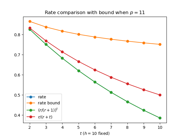
Let (and thus locality ) be fixed and set to maximize the number of recovery sets for each field size. For each , let take on the maximum value guaranteeing positive minimum distance in Theorem 3.4. In Figure 5.1 we graph the rates of codes over for , increasing field size as well as number of recovery sets. We also graph the proven and conjectured rate bounds for codes with this availability and locality from [10]. The lengths of the codes are quite large, so we omit the accompanying tables. We find that the rate of the constructed codes is close to the product code rate for all , growing extremely close as increases. When we examine the minimum distance of these codes, we find that, in all cases except , the minimum distance of the constructed code is larger than that of the corresponding product code and the Wang et al. construction. However, this minimum distance comes at a cost of greater length and working over a larger field.
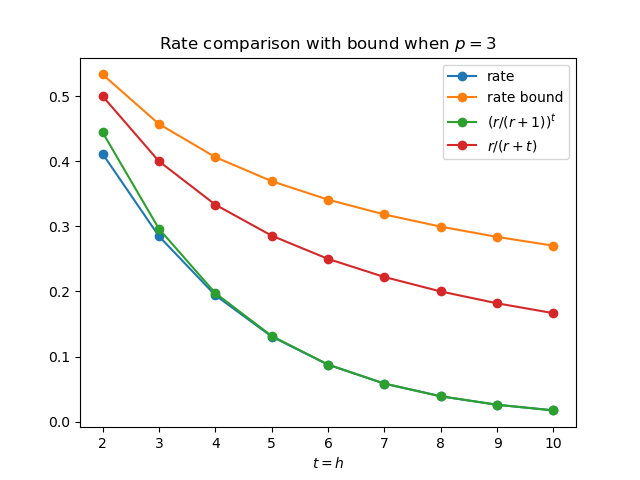
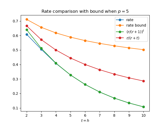
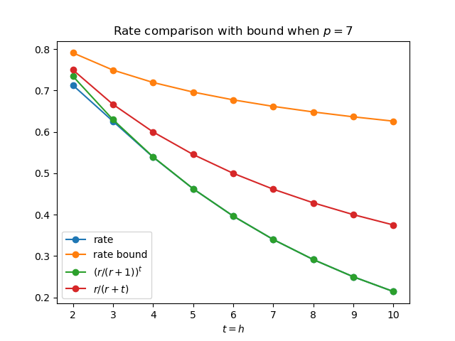
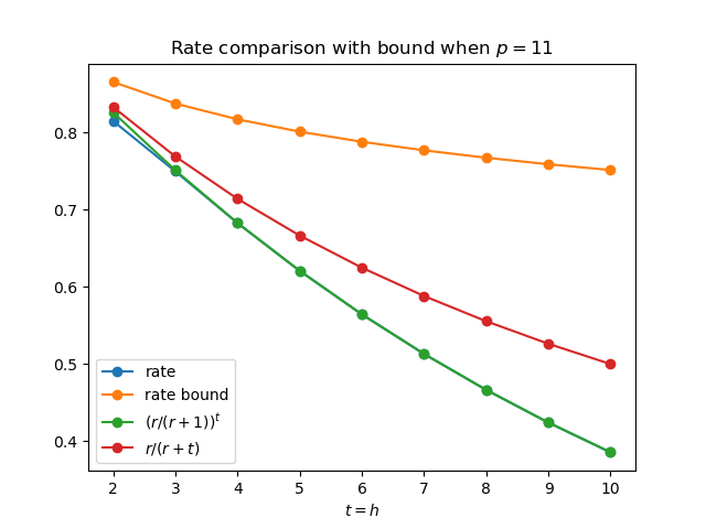
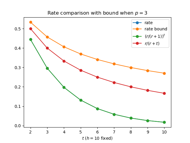
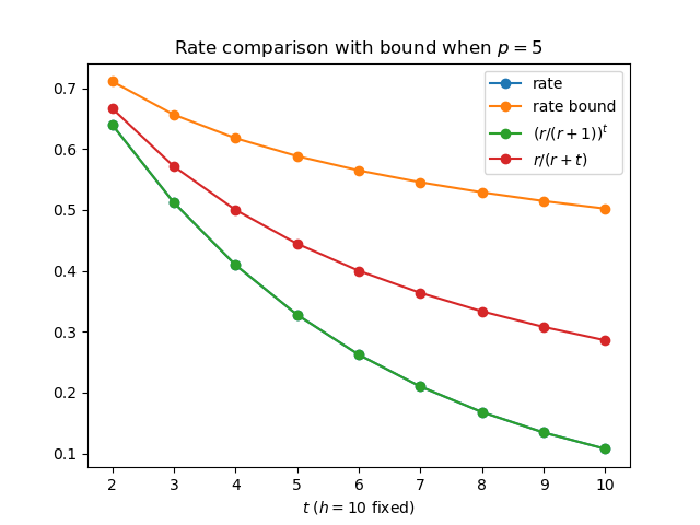
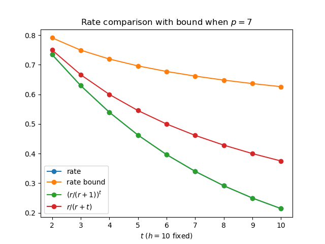
One might wonder what happens when field size and locality are fixed, but the number of factor curves (and recovery sets) is increased. In Figure 5.2, we graph the rate of the code over , where is maximized for guaranteed positive minimum distance, as well as the proven rate bound from (5.1) and the rates of the Tamo-Barg product construction and Wang et al. construction, for . The lengths of the codes are quite large, so we omit the accompanying tables. We find that the rate of the fiber product codes is extremely close to the product code construction bound, matching up to at least 4 decimal places in each case. The lower bound on minimum distances of these codes are also larger than that of the product code and Wang et al. construction when is not . This larger minimum distance comes at a cost of much greater length, however; the relative minimum distance of the fiber product codes is less than either of the other constructions.
5.4.5 Rate for Fixed as Locality Increases
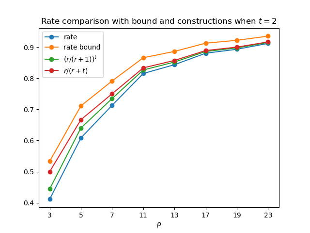
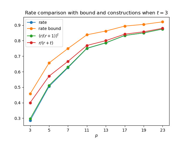
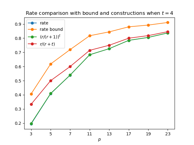
Finally, we consider the parameters of the codes for various fixed values of as the prime increases and is chosen to maximize rate while guaranteeing positive minimum distance. Notice that the field size in each case is so this increases with and . In Figure 5.3
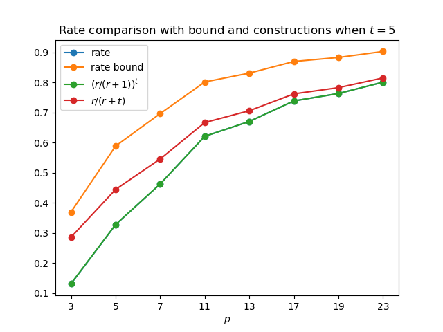
5.4.6 Comparison with Product Code Rate as Locality Increases
We now consider the actual formula for the rate of when is chosen for maximal rate with positive minimum distance. Recall that the length and dimension of are given by
With some simplification, this gives a rate at least
As increases, we see that
Thus at increases, the rate of approaches 1. Further, the rate of is asymptotically the same as the rate of the corresponding product code (here, , so the product code with matching locality and availability would have rate ). Asymptotically, the Wang et al. construction grows at the same rate as well. Again, the product code and Wang et al. constructions both have the advantage of smaller field size.
References
- [1] SB Balaji, M Nikhil Krishnan, Myna Vajha, Vinayak Ramkumar, Birenjith Sasidharan, and P Vijay Kumar. Erasure coding for distributed storage: An overview. Science China Information Sciences, 61(10):1–45, 2018.
- [2] Alexander Barg, Itzhak Tamo, and Serge Vlăduţ. Locally recoverable codes on algebraic curves. IEEE Transactions on Information Theory, 63(8):4928–4939, 2017.
- [3] Daniele Bartoli, Maria Montanucci, and Luciane Quoos. Locally recoverable codes from automorphism group of function fields of genus . IEEE Transactions on Information Theory, 66(11):6799–6808, 2020.
- [4] Sourbh Bhadane and Andrew Thangaraj. Unequal locality and recovery for locally recoverable codes with availability. In 2017 Twenty-third National Conference on Communications (NCC), pages 1–6, 2017.
- [5] Kathryn Haymaker, Beth Malmskog, and Gretchen L Matthews. Locally recoverable codes with availability t2 from fiber products of curves. Advances in Mathematics of Communications, 12(2):317, 2018.
- [6] Swanand Kadhe and Robert Calderbank. Rate optimal binary linear locally repairable codes with small availability. In 2017 IEEE International Symposium on Information Theory (ISIT), pages 166–170, 2017.
- [7] Carlos Munuera and Wanderson Tenório. Locally recoverable codes from rational maps. Finite Fields and Their Applications, 54:80–100, 2018.
- [8] Carlos Munuera, Wanderson Tenório, and Fernando Torres. Locally recoverable codes from algebraic curves with separated variables. Advances in Mathematics of Communications, 14(2):265–278, 2020.
- [9] Henning Stichtenoth. Algebraic function fields and codes, volume 254. Springer Science & Business Media, 2009.
- [10] Itzhak Tamo and Alexander Barg. Bounds on locally recoverable codes with multiple recovering sets. 2014 IEEE International Symposium on Information Theory, pages 691–695, 2014.
- [11] Itzhak Tamo and Alexander Barg. A family of optimal locally recoverable codes. IEEE Transactions on Information Theory, 60(8):4661–4676, 2014.
- [12] Itzhak Tamo, Alexander Barg, and Alexey Frolov. Bounds on the parameters of locally recoverable codes. IEEE Transactions on Information Theory, 62(6):3070–3083, 2016.
- [13] Gerard van der Geer and Marcel van der Vlugt. How to construct curves over finite fields with many points. In Arithmetic geometry, Symposia Mathematica XXXVII, pages 169–189, Cambridge, 1997. Cambridge University Press.
- [14] Anyu Wang, Zhifang Zhang, and Mulan Liu. Achieving arbitrary locality and availability in binary codes. In 2015 IEEE International Symposium on Information Theory (ISIT), pages 1866–1870, 2015.