MOA-2020-BLG-135Lb: A New Neptune-class Planet for the Extended MOA-II Exoplanet Microlens Statistical Analysis

Abstract

We report the light-curve analysis for the event MOA-2020-BLG-135, which leads to the discovery of a new Neptune-class planet, MOA-2020-BLG-135Lb. With a derived mass ratio of $q=1.52_{-0.31}^{+0.39}\times 10^{-4}$ and separation $s\approx 1$, the planet lies exactly at the break and likely peak of the exoplanet mass-ratio function derived by the MOA collaboration (Suzuki et al., 2016). We estimate the properties of the lens system based on a Galactic model and considering two different Bayesian priors: one assuming that all stars have an equal planet-hosting probability and the other that planets are more likely to orbit more massive stars. With a uniform host mass prior, we predict that the lens system is likely to be a planet of mass $m_{\mathrm{planet}}=11.3_{-6.9}^{+19.2}M_{\oplus}$ and a host star of mass $M_{\mathrm{host}}=0.23_{-0.14}^{+0.39}M_{\odot}$, located at a distance $D_{L}=7.9_{-1.0}^{+1.0}\;\mathrm{kpc}$. With a prior that holds that planet occurrence scales in proportion to the host star mass, the estimated lens system properties are $m_{\mathrm{planet}}=25_{-15}^{+22}M_{\oplus}$, $M_{\mathrm{host}}=0.53_{-0.32}^{+0.42}M_{\odot}$, and $D_{L}=8.3_{-1.0}^{+0.9}\;\mathrm{kpc}$. This planet qualifies for inclusion in the extended MOA-II exoplanet microlens sample.

latexA float is stuck

1 Introduction

Gravitational microlensing (Mao & Paczynski, 1991) has been solidified as one of the main techniques for detecting planets, being most sensitive to low-mass planets (Bennett & Rhie, 1996) that orbit at moderate to large distances from their host star (Gould & Loeb, 1992), typically from $0.5\text{-}10\,\text{AU}$, complementing other exoplanet detection methods (Bennett, 2008; Gaudi, 2012; Batista, 2018; Guerrero et al., 2021). The first planetary microlensing event was discovered in 2004 (Bond et al., 2004), and since then, more than 120 exoplanets have been discovered by the method of gravitational microlensing.

The most recent statistical analysis of planetary signals discovered using gravitational microlensing implied that cold Neptunes were likely to be the most common type of planets beyond the snow line (Suzuki et al., 2016). This inference was done by discovering a break and likely peak in the planet–to–host star mass-ratio function for a mass ratio $q\sim 10^{-4}$ when studying the MOA-II microlensing events from 2007 to 2012. At the time of that statistical analysis, it was possible to conclude that while the Suzuki et al. (2016) sample generally supported the predictions for the planet distribution from core accretion theory population synthesis models for planets beyond the snow line (Ida & Lin, 2004; Mordasini et al., 2009), the existence of this Neptune peak in the sample distribution actually added contradictions. These previous models for the planet distribution predicted the existence of a sub-Saturn mass planet desert, which conflicted with the microlensing observations (Suzuki et al., 2016, 2018). Only this year Ali-Dib et al. (2022) published their investigation into the origins of cold sub-Saturns, which concluded that these exoplanets may be more common than what was previously predicted. It is important to notice that the Suzuki et al. (2016) sample had only 30 exoplanets, which makes the expansion of this sample crucial for future investigations and, consequently, for a better understanding of the distribution of exoplanets.

In this paper, we present the analysis of the gravitational microlensing event MOA-2020-BLG-135 with a short-term planetary lensing signal in its light curve. This analysis leads us to the discovery of MOA-2020-BLG-135Lb, a new planet detected by MOA-II. This new exoplanet qualifies to be included in the upcoming statistical analysis of cold exoplanets detected by the MOA-II survey, which is the expansion of the Suzuki et al. (2016) sample analysis. This paper, presenting a complete study of this event, is organized as follows. First, we describe the observation of the event in Section 2, and how we obtain our best-fit models and explore the full parameter space in Section 3. Then, we explain the photometric calibration and how we retrieve the source size in Section 4, and present our methodology to estimate the lens’s physical properties in Section 5, and discuss them comparing with previous literature in Section 6. Finally, we conclude summarizing our results in Section 7.

2 Observations and Data

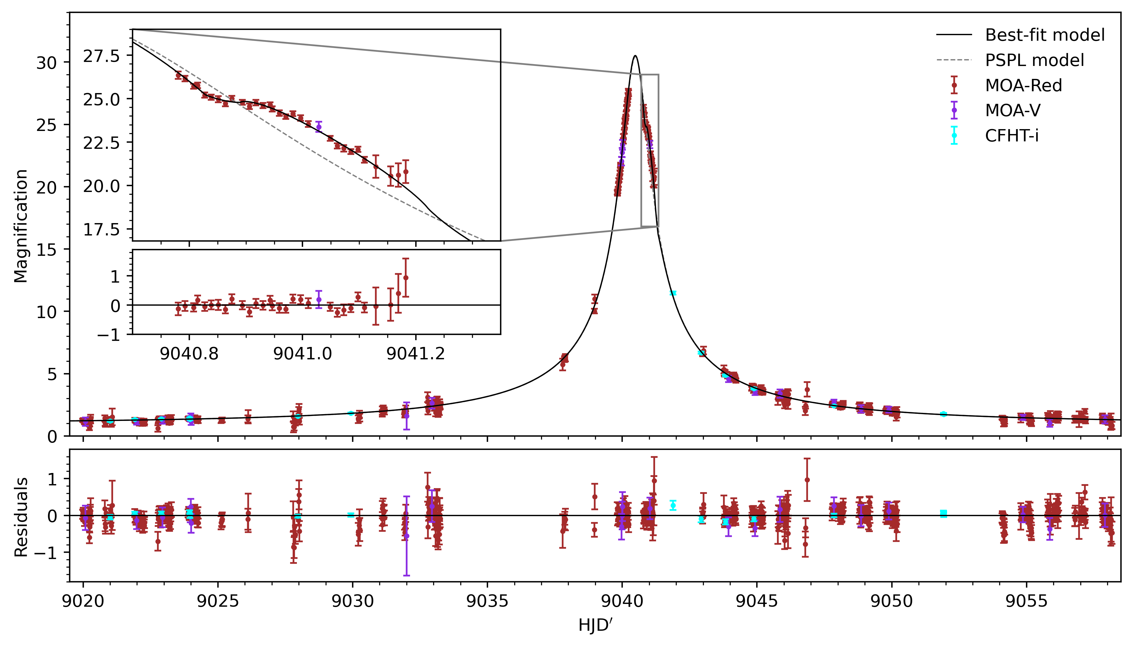
Figure 1: The best-fit model for the MOA-2020-BLG-135 light curve in a time ($\mathrm{HJD^{\prime}}=\mathrm{HJD}-2,450,000$) vs. magnification plot. The MOA-Red, MOA-V, and CFHT-i data are shown in brown, violet, and blue, respectively. The best single source planetary model 2L1S (i.e., two lenses and one source) $s>1$ is our best-fit model (see Section 3) and is displayed as a black solid line, while the Point-Source Point-Lens (PSPL) model is displayed as a dashed gray line. The main panel shows all the photometric data sets overlaid with the best-fit model. The upper left side of the Figure, zooming near the peak of the event, shows the planetary perturbation, which is well covered by the MOA-Red data set, and the corresponding residuals. The lower panel shows the residuals of the best-fit model for each instrument - see colored legend.

The microlensing event MOA-2020-BLG-135 was discovered by the Microlensing Observations in Astrophysics (MOA) collaboration and first alerted on 2020 July 7. This event was located at the J2000 equatorial coordinates $\left(\mathrm{R.A.,\ decl.}\right)=(17^{\mathrm{h}}\,53^{\mathrm{m}}\,41\overset{{}^{\mathrm{s}}}{.}64,\ -29\arcdeg 48\arcmin\,27\overset{\prime\prime}{.}\,24)$, and Galactic coordinates $(l,\,b)=(0.15598\arcdeg,\,-1.95678\arcdeg)$ in the MOA-II field ‘gb5’ (Sumi et al., 2013). The MOA observations were performed using the purpose-built 1.8m wide-field MOA telescope located at Mount John Observatory, New Zealand, and the observations of the field ‘gb5’ were taken with a 15-minute cadence using the MOA-Red filter. The MOA-Red filter corresponds to a customized wide-band similar to a sum of the Kron-Cousins R and I bands, from $600\;\mathrm{nm}$ to $900\;\mathrm{nm}$. Occasional observations from the MOA group were made in the visual band using the MOA-V filter. The photometry in these filters was initially performed in real-time by the MOA pipeline (Bond et al., 2001), based on the difference imaging method (Tomaney & Crotts, 1996). The data used in this paper are from a re-reduction done using the Bond et al. (2017) method, which performs a detrending process to correct for systematic errors and removes correlations in the data that may be present due to variations in the seeing and effects of differential refraction (Bennett et al., 2012; Bond et al., 2017). The Bond et al. (2017) method also provides photometry calibrated to the Optical Gravitational Lensing Experiment phase III project (OGLE-III) (Szymański et al., 2011).

The Canada–France–Hawaii Telescope (CFHT), located near the summit of Mauna Kea in Hawaii, United States, also observed the event in the SDSS $i$-band filter. From 2020 March to July, CFHT provided 1-2 supplementary observations per night toward the Korea Microlensing Telescope Network (KMTNet) high-cadence fields and follow-up observations for high-magnification events (Zang et al., 2021). The CFHT data contributes to the establishment of the baseline brightness of the source after the anomaly, and covers a two-day gap with a data point at $\mathrm{HJD}=2,459,041.9$. The CFHT data were reduced by a custom difference imaging analysis pipeline (Zang et al., 2018) based on the ISIS package (Alard & Lupton, 1998; Alard, 2000).

The MOA-2020-BLG-135 event was also alerted one day later by the Korea Microlensing Telescope Network (KMTNet) group as KMT-2020-BLG-0579. The KMTNet collaboration monitored this event with the 1.6m telescope located at the Siding Spring Observatory, Australia (Kim et al., 2016). Unfortunately, in addition to the KMTNet data not covering the anomaly, evidence of systematics was found in their data. Since the data would not improve the characterization of the main event and the planet, the KMTNet team suggested removing their data from the paper.

As a result of observatories’ shutdowns due to the COVID-19 pandemic, data from KMT Cerro Tololo Interamerican Observatory, in Chile, KMT South African Astronomical Observatory, in South Africa, and OGLE, in Chile, could not be taken. These observatories were closed when the microlensing event happened.

Figure 1 shows the three datasets used for the analysis of this event. MOA-Red data and the MOA-V data are displayed respectively in brown and violet colors, and the CFHT-i data are in blue.

3 Light-curve Models

The light curve for the MOA-2020-BLG-135 event (see Figure 1) looks similar to a Paczyński curve (Paczynski, 1986), except for the anomaly in the interval $\mathrm{HJD^{\prime}}=[9040.7,9041.5]$ observed by both MOA-Red and MOA-V (zoomed in Figure 1). The Paczyński curve assumes a model in which the lens consists of a single star and the radiant flux comes from a single source. We display this curve as a point-source point-lens (PSPL) model in Figure 1. This deviation indicates that the lens may be composed of two masses, in which the less massive lens component can be a planet-mass object. We call this a binary or planetary lens system, depending on the mass ratio, as there are two objects contributing gravitationally as lenses. In Section 3.1, we search for a lensing model explaining the three data sets presented in Section 2 (MOA-Red, MOA-V, and CFHT-i) by exploring the parameter space of possible binary lenses with a single source (2L1S) using the method described in Bennett (2010). In Section 3.2, we propose the lack of evidence for a binary-source model - with single lens (1L2S) or binary lens (2L2S) - after investigating the light curve using the method described in Bennett et al. (2018).

3.1 Single Source Scenario

The Bennett (2010) process uses the image-centered, ray-shooting method (Bennett & Rhie, 1996) combined with a custom version of the Metropolis algorithm (Metropolis et al., 1953), which yields a rapid convergence to a $\chi^{2}$ minima.

3.1.1 Fit Parameters

The parameters of our model are: the Einstein crossing time ($t_{\mathrm{E}}$); the time at which the separation of lens and source reaches the minimum ($t_{0}$); the minimum angular separation between source and lens as seen by the observer ($u_{0}$); the separation of the two masses of the binary lens system during the event ($s$); the counterclockwise angle between the lens-source relative motion projected onto the sky plane and the binary lens axis ($\alpha$); the mass ratio between the secondary lens and the primary lens ($q$); the source radius crossing time ($t_{*}$); the source flux for each instrument $i$ ($f_{s,i}$); and the blend flux per instrument $i$ ($f_{b,i}$).

The parameters $t_{\mathrm{E}}$, $t_{0}$ and $u_{0}$ are the common parameters for the single-lens model, while $s$, $\alpha$ and $q$ are the additional parameters for a binary lens system model. Both length parameters, $u_{0}$ and $s$, are normalized by the angular Einstein radius $\theta_{\mathrm{E}}$, defined by

$$\theta_{\mathrm{E}}=\sqrt{\frac{4GM_{L}}{c^{2}D_{S}}\left(\frac{D_{S}}{D_{L}}-1\right)},$$ (1)

where $G$ is the gravitational constant, $M_{L}$ is the mass of the lens system, $c$ is the speed of light, $D_{S}$ is the observer-source distance, and $D_{L}$ is the observer-lens distance. The source radius crossing time, $t_{*}$, is included in the lensing model to take account of finite source effects,

$$t_{*}=\rho\>t_{\mathrm{E}}=\frac{\theta_{*}}{\theta_{\mathrm{E}}}t_{\mathrm{E}},$$ (2)

where $\rho$ is the source angular radius in Einstein units, and $\theta_{*}$ is the source angular radius.

The other two parameters taken into account are the blend flux $f_{b,i}$ and the source flux $f_{s,i}$. As microlensing events are observed in crowded stellar fields, the source is usually blended with other unlensed stars. For this reason, we consider the blend flux. Since the observed brightness has a linear dependence on the blend flux and the source flux, they are treated differently from the other nonlinear fit parameters, as it follows. For every instrument and each set of the previously cited fit parameters, we can find a total flux that minimizes the $\chi^{2}$. The total flux $F_{i}(t)$ for time $t$ for instrument $i$ can be written as:

$$F_{i}(t)=A(t,\textbf{x})\>f_{s,i}+f_{b,i},$$ (3)

where $A(t,\textbf{x})$ is the magnification of the event at any given time and for any given set of nonlinear parameters $\textbf{x}=(t_{\mathrm{E}},t_{0},u_{0},s,\alpha,q,t_{*})$, $f_{s,i}$ is the unlensed source flux in a specific passband $i$, and $f_{b,i}$ is its excess flux. For many light curves reduced with difference imaging, the blend flux has an arbitrary normalization. Yet, the Bond et al. (2017) method normalizes the total flux to match the flux of the nearest star-like object in the reference frame, and it is the one used for the MOA data.

For this modeling, we do not consider parallax effects because this is a short ($t_{\mathrm{E}}\approx 17\;\mathrm{days}\ll 1\;\mathrm{month}$) and faint event. Additionally, its peak of magnification was reached on 2020 July 10, when the Earth’s instantaneous acceleration toward the projected position of the Sun projected into the lens plane was close to its minimum. These three factors make it very unlikely to detect asymmetric features in the light curve tails due to parallax effect. Therefore, we do not attempt a parallax measurement for this event.

3.1.2 Exploring the Full Parameter Space

Table 1: Best-fit Model Parameters for MOA-2020-BLG-135, and Corresponding Averages from the Posterior Distribution

Parameters	Units	2L1S $s<1$	2L1S $\mathbf{s>1}$	MCMC Averages	$2\sigma$ Range
$t_{\mathrm{E}}$	days	$16.905$	$16.791$	$16.85_{-0.27}^{+0.28}$	$16.30$-$17.41$
$t_{0}$	$\mathrm{HJD^{\prime}}$	$9040.48797$	$9040.48843$	$9040.4879_{-0.0019}^{+0.0020}$	$9040.4839$-$9040.4920$
$u_{0}$		$0.03260$	$0.03287$	$0.03275_{-0.00072}^{+0.00072}$	$0.03134$-$0.03421$
$s$		$0.95472$	$1.04509$	$0.997_{-0.054}^{+0.096}$	$0.916$-$1.126$
$\alpha$	radians	$2.38728$	$2.37731$	$2.383_{-0.013}^{+0.021}$	$2.360$-$2.433$
$q$	$10^{-4}$	$1.55314$	$1.13963$	$1.52_{-0.31}^{+0.39}$	$1.01$-$2.47$
$t_{*}$	days	$0.14661$	$0.14186$	$0.145_{-0.011}^{+0.018}$	$0.125$-$0.183$
$I_{S}$		$19.009$	$19.000$	$19.004_{-0.045}^{+0.045}$	$18.914$-$19.095$
$V_{S}$		$21.137$	$21.127$	$21.132_{-0.045}^{+0.045}$	$21.042$-$21.223$
fit $\chi^{2}$		$14819.9$	$14819.7$	…	…

We start modeling by systematically exploring the full parameter space with the grid-search approach described in Bennett (2010). For the first step, we do an initial condition grid search where $t_{\mathrm{E}}$, $t_{0}$, $u_{0}$, and $t_{*}$ are fixed, while $s$, $\alpha$, and $q$ are scanned. This is done so we can select the initial conditions. From there, we use the custom version of the Metropolis algorithm, as implemented by Bennett (2010), with initial positions coming from the 13 local solutions obtained from these initial scans. To ensure that no good model is missed in our analysis, we make sure that different mass ratios in the $q\in[10^{-5},10^{-1}]$ range are included in our set of initial conditions. Our customized Metropolis algorithm provides a full fit, in which all the parameters are free. Then, we select the best-fit model by looking for the lowest $\chi^{2}$, which indicates a model with $q\sim 10^{-4}$.

Interpreting a planetary lensing event with a planet signal is often subject to a close-wide degeneracy, in which a solution with a certain separation $s$ results in a similar model to another model presenting a solution with the same parameters’ values but with a separation given by $1/s$. This degeneracy arises from the symmetries in the lens equation (Griest & Safizadeh, 1998; Dominik, 1999). As discussed in Yee et al. (2021), the degeneracy appears even for resonant caustics, which are far from the $s\gg 1$ limit in which the symmetries were derived. Therefore, we carefully cover both the close ($s<1$) and the wide ($s>1$) solutions in our analysis.

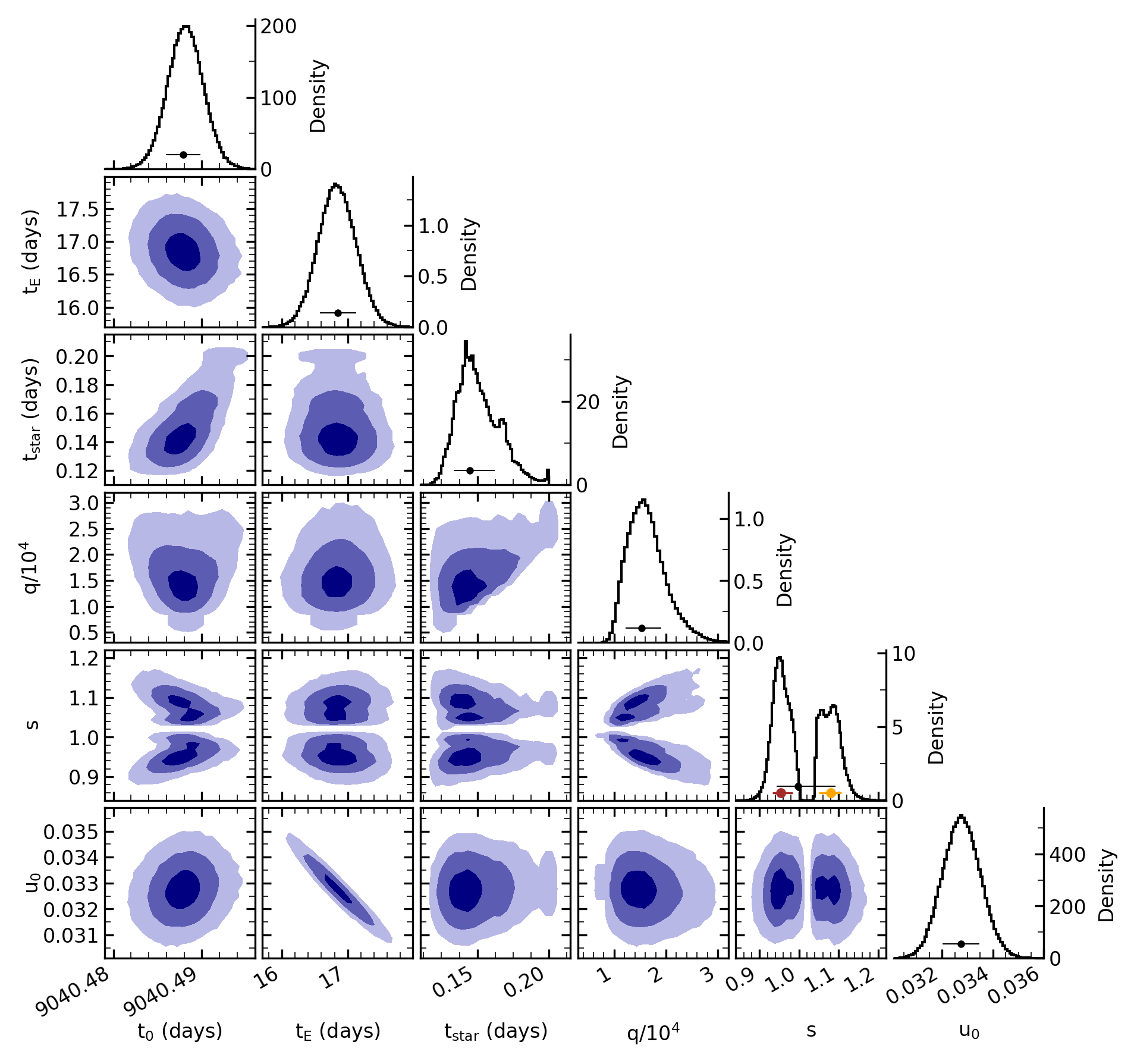
Figure 2: The marginalized posterior distributions for our MCMC runs, correlating the parameters for the binary lens single source model (2L1S), and, in the diagonal, the 1-dimension Probability Density Function (PDF) of each parameter. The $68.3\%$ (1$\sigma$), $95.5\%$ (2$\sigma$), and $99.7\%$ (3$\sigma$) confidence intervals are shown in dark blue, median blue, and light blue, respectively, in the posterior distribution plots. In the PDF plots, the black dot points out the median, and the thin line marks the 1$\sigma$ confidence interval. For the separation $s$ PDF plot, the additional red and yellow dots and lines also point out the median and the 1$\sigma$ confidence interval, but now for each of the two regions, the close-separation ($s<1$) in red and the wide-separation ($s>1$) in yellow.

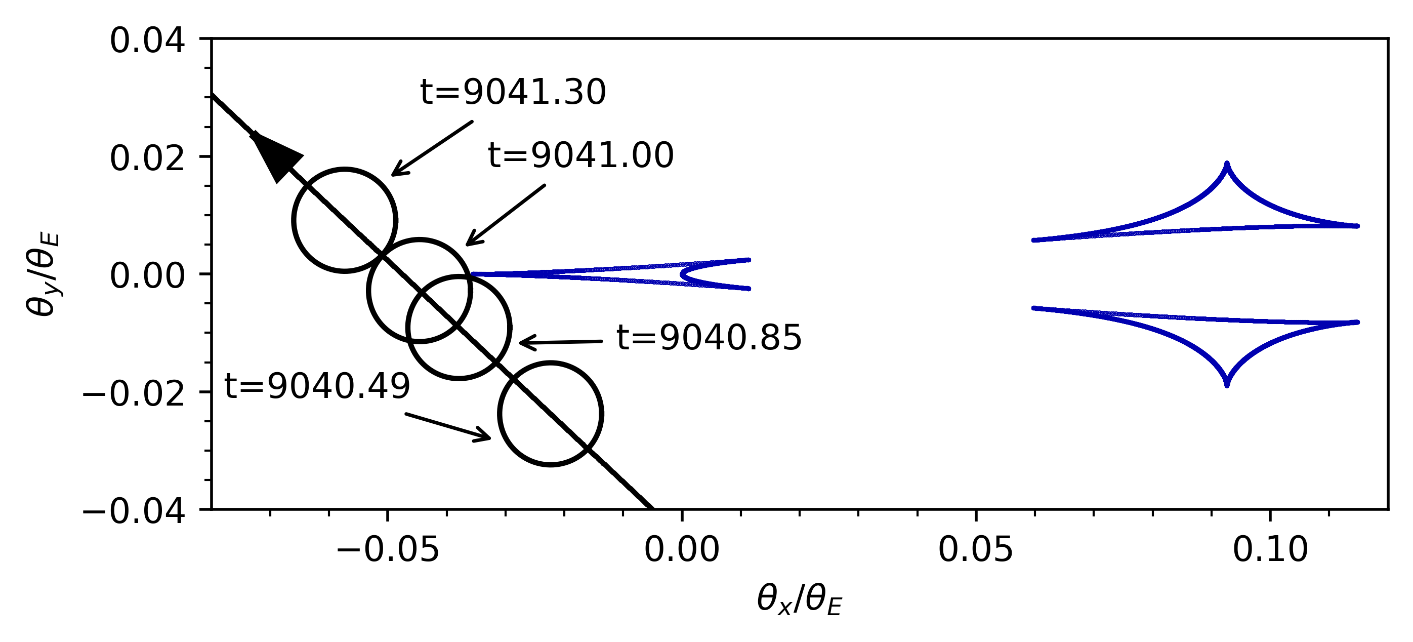
(a)

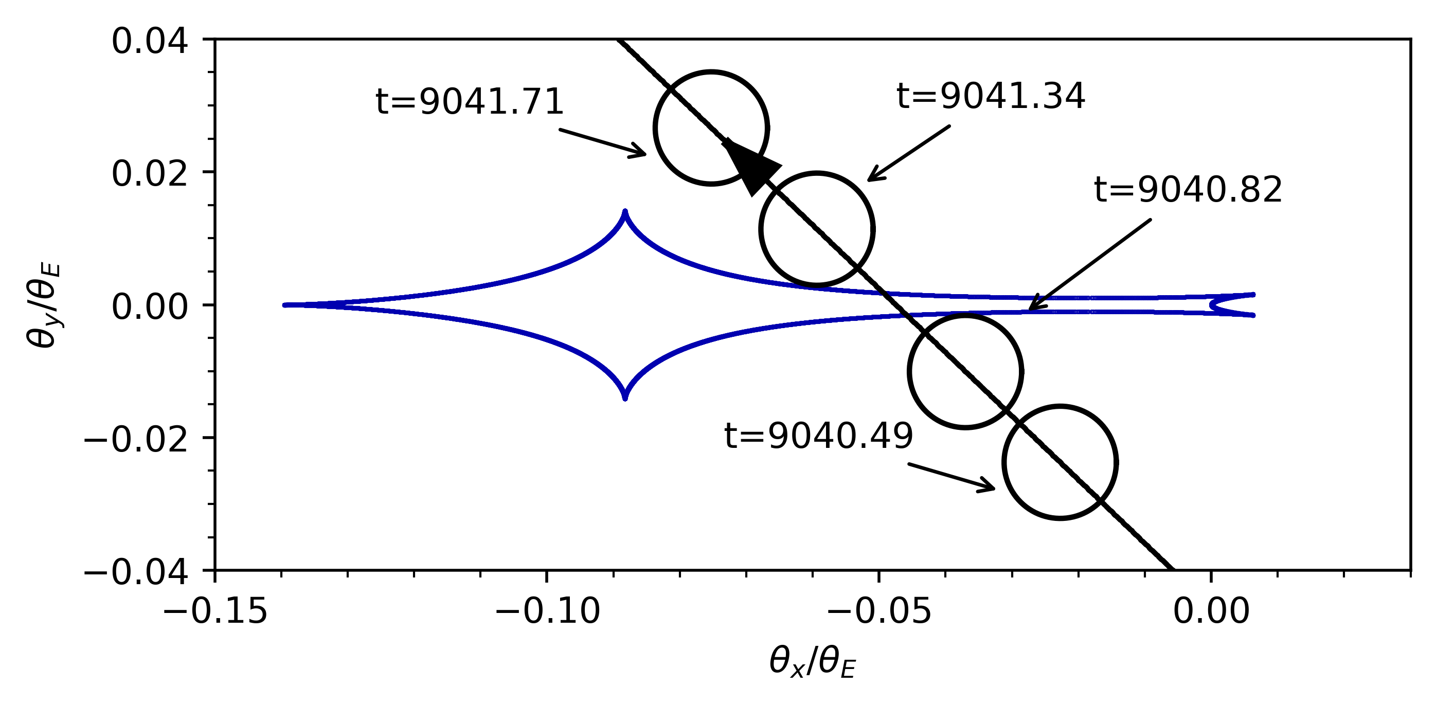
(b)

Figure 3: The caustic geometry and the source-lens trajectory. The caustic is represented in blue. The black straight solid line shows the source-lens trajectory and the arrow shows the direction of the source-lens relative motion. The source size is displayed as a black circle at its position at $\mathrm{HJD^{\prime}}=9040.49$ (event peak), $\mathrm{HJD^{\prime}}=9040.85$ for $s<1$ and $\mathrm{HJD^{\prime}}=9040.82$ for $s>1$(source starts crossing the caustic), and $\mathrm{HJD^{\prime}}=9041.00$ for $s<1$ and $\mathrm{HJD^{\prime}}=9041.34$ for $s>1$ (source exiting the caustic). For (b), the source at $\mathrm{HJD^{\prime}}=9041.71$ is also displayed to show when it is closest to the upper cusp.

To guarantee the exploration of the full parameter space with the Monte Carlo method, we use our customized version of the Metropolis algorithm for both the close and wide solutions. When running the Markov Chain Monte Carlo (MCMC) algorithm with the parameters of the best-fit models as initial inputs, we notice that the proposal distribution function we choose allows each chain to jump back and forth between the wide and close solutions. This happens because both values for the separation $s$ are close enough that the $\chi^{2}$-barrier between them has a size encompassed by the possible jumps. To ensure the optimization of the posterior sampling, we conduct MCMC runs adjusting the variables for our diagonalized covariance matrix and combine the results of the runs. For our analysis, we combine only the MCMC runs that jump between the wide and close solution, and vice-versa, and those have chains with a similar best-fit model.

Our best-fit planetary light curve model (2L1S $s>1$) is shown in Figure 1, and its parameters are given in Table 1, being the solution referred to as simply “the best-fit model” in this paper. The result of our best-fit model for 2L1S $s<1$ is also displayed in Table 1. The median of the marginalized posterior distributions with the 1$\sigma$ confidence interval (i.e., $68.3\%$) is displayed in the same table, together with the range for distributions within the 2$\sigma$ interval (i.e., $95.5\%$). Figure 2 shows the posterior distribution together with the 1$\sigma$, 2$\sigma$, and 3$\sigma$ (i.e., $99.7\%$) confidence intervals.

In Figure 2, a butterfly-wing shape is visible in the posterior distribution for $s$. This shape shows that both the close and wide solutions were fully explored during our MCMC runs. This is an effect from our algorithm jumping back and forth in between both wide and close solutions. Even though there seems to exist two regions in each butterfly wing when considering the 1$\sigma$ interval, the chi-square difference is not big enough to create a barrier that could separate them into four defined regions.

Figure 3a and Figure 3b illustrate the close-separation ($s<1$) and the wide-separation ($s>1$) topology, respectively. We can see in Figure 3 that, although the topology of the caustics for each solution has a different shape, the source trajectory crosses parts with slightly similar shapes of both caustics. An (2021) argues that local degeneracies of lensing features associated with caustic crossings can still exist in the planetary events even in situations in which the overall caustic shape may not be degenerate at all. As a consequence, for our data points, the best-fit model for the light curve with the planetary separation solution $s>1$ is practically the same as the one for the solution $s<1$. For $s<1$, the anomaly due to the planet presence appears to start at $\mathrm{HJD^{\prime}}\approx 9040.85$, finishing at $\mathrm{HJD^{\prime}}\approx 9041.30$, while for $s>1$, it appears to start at $\mathrm{HJD^{\prime}}\approx 9040.82$, finishing at $\mathrm{HJD^{\prime}}\approx 9041.34$. The explanation of these small differences can be found in Figure 3, which indicates the source starts and finishes crossing the caustic at different time. Moreover, we can check the great similarity for all the fitting parameters, together with both $s$ being close to the inverse of each other, indicating the close-wide degeneracy solutions. One might wonder about the proximity of the source and the upper cusp at $\mathrm{HJD^{\prime}}\approx 9041.71$ in the lower panel of Figure 3. This upper cusp does not seem to create an extra perturbation, and it is located far from the source, more than one source radius away at $\mathrm{HJD^{\prime}}\approx 9041.71$. It results in no apparent anomaly in the best-fit model in Figure 1.

3.2 Binary Source Possibility

The investigation of the possibility of two sources was encouraged when still considering using the KMTNet data. However, the evidence of binary source largely disappeared when systematic of KMTNet data was discovered.

Following the suggestion of the KMTNet collaboration, we remove the KMTNet data from the analysis, as explained in Section 2, and we attempt to fit binary source models to our data. We use the method described in Bennett et al. (2018) to look for, first, solutions with binary-source single-lens (1L2S) and, then, with binary-source binary-lens (2L2S) models. For easier comparison, we refer to the Point-Source Point-Lens (PSPL) model as PSPL/1L1S, the best-fit model as 2L1S $s>1$, and its degenerate model as 2L1S $s<1$ (Section 3.1).

The Bennett et al. (2018) method allows us to add a second source with different brightness and color from the first source. We find the best-fit for the 1L2S model to have a fit $\chi^{2}=14862.24$, with a lens-source proper motion of $\mu_{\mathrm{rel,G}}=0.44\pm 0.05\mathrm{\;mas\;yr^{-1}}$, which is unusually small. With $\Delta\chi_{\mathrm{1L2S-2L1S}}^{2}=42.53$ and a small relative proper motion, our results indicate a strong preference toward the 2L1S $s>1$ model. Therefore, the 1L2S model is ruled out because it suggests that a model with a second source and only one lens reduces the quality of the fitting to the data.

For the binary-source binary-lens, 2L2S, model, we include the binary-lens parameters. We obtain a fit $\chi^{2}=14807.54$, which is smaller than the one for the 2L1S $s>1$ model ($\Delta\chi_{\mathrm{2L1S-2L2S}}^{2}=-12.17$). As expected, due to a larger number of parameters, a model with 2L2S may improve the $\chi^{2}$, so an extra criterion is necessary to evaluate the significance of this small improvement. Therefore, we also calculate the Bayesian Information Criterion (BIC) (Schwarz, 1978) indexes for the two models. The difference in BIC index is $\Delta\mathrm{BIC}_{\mathrm{2L2S-2L1S}}=35.85$. The improvement of the quality of the fit is, then, proved to be insignificant when using the BIC index. Moreover, it should be noted that a binary source event requires special alignment of the sources, being generally unlikely to be detected. Therefore, we continue our analysis considering only the 2L1S model.

The differences in $\chi^{2}$ and BIC index for each model compared to our best-fit model is displayed in Table 2.

Table 2: Comparison Between Microlensing Models

Model	$N_{\mathrm{parameters}}$	$\Delta\chi^{2}$	$\Delta\mathrm{BIC}$
PSPL/1L1S	3	669.28	630.87
1L2S	8	42.53	52.13
2L1S s $<$ 1	7	0.21	0.21
2L1S $\mathbf{s>1}$	7	…	…
2L2S	12	-12.17	35.85

4 Photometric Calibration and Source Properties

The source angular radius $\theta_{*}$ is not explicitly obtained from the lightcurve models presented in Section 3, yet it can be empirically derived if we know the de-reddened magnitude and color of the source (Van Belle, 1999; Yoo et al., 2004; Bennett, 2010). Toward this aim, we correct the extinction and reddening for the source star by using the red clump giants as a reference.

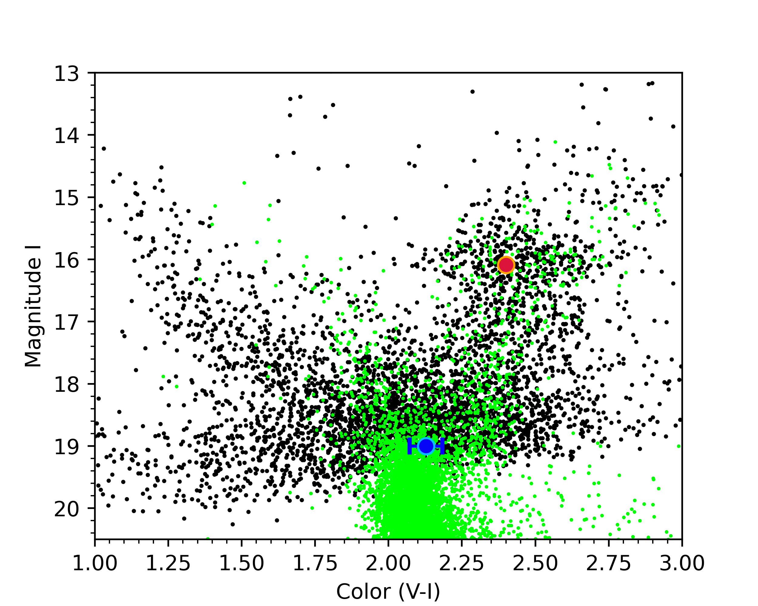
Figure 4: (V - I, I) Color-magnitude diagram of the stars in the OGLE-III catalog within $90^{\prime\prime}$ of MOA-2020-BLG-135. The black dots are the stars from the OGLE-III catalog, the blue dot indicates the source magnitude and color for the best-fit model ($s>1$), and the red circle indicates the red clump giant centroid. For comparison, we added the green dots showing the Hubble Space Telescope CMD from Holtzman et al. (1998) shifted to the bulge distance and relevant extinction derived in Section 4. The source star is probably in a subgiant phase.

In order to obtain the dereddened color and corrected magnitude of our source star, we first calibrate the instrumental MOA-II magnitudes, MOA-Red and MOA-V, with the OGLE-III catalog considering the following equations from a standard calibration procedure described in Bond et al. (2017):

$$I_{\mathrm{O3}}=(28.0983\pm 0.0014)+R_{MOA}\\ -(0.20844\pm 0.00087)\times(V_{MOA}-R_{MOA})\\$$ (4)

$$V_{\mathrm{O3}}=(28.5038\pm 0.0014)+V_{MOA}\\ -(0.10746\pm 0.00088)\times(V_{MOA}-R_{MOA}),$$ (5)

where $R_{\mathrm{MOA}}$ is the MOA-Red filter and $V_{\mathrm{MOA}}$ is the MOA-V filter. We then obtain the magnitude $I_{\mathrm{O3}}$ and $V_{\mathrm{O3}}$ (Gould et al., 2010) for our source star. These are displayed in Table 1 as $I_{\mathrm{S}}$ and $V_{\mathrm{S}}$ respectively. Figure 4 shows the calibrated color and magnitude for our source star, compared to the stars within a $90^{\prime\prime}$ radius limit from our target.

For the second step, we measure the extinction and reddening of the stars within a $90^{\prime\prime}$ radius limit from our source star as follows. First, we calculate what are the apparent magnitude and color of the red clump, obtaining $I_{\mathrm{RCG}}=(16.09\pm 0.05)$ and $(V-I)_{\mathrm{RCG}}=(2.40\pm 0.05)$ (represented as the red dot in Figure 4). The expected dereddened magnitude of the red clump at a Galactic longitude $l=0.15598\arcdeg$ is $I_{\mathrm{RCG,0}}=(14.44\pm 0.04)$ (Nataf et al., 2013), and the expected color is $(V-I)_{\mathrm{RCG,0}}=(1.06\pm 0.06)$ (Bensby et al., 2011). Therefore, we can use the calculated apparent magnitude and color of the red clump in comparison with the expected values to obtain the extinction and the color excess of this region in the sky. The extinction and the color excess are: $A_{\mathrm{I}}=(1.65\pm 0.06)$ and $E(V-I)=(1.34\pm 0.08)$. These values are reasonable, and can be compared to the ones given by the OGLE-III tool for querying interstellar extinction toward the Galactic bulge , which were $A_{\mathrm{I}}=1.60$ and $E(V-I)=1.35$ when using the natural neighbor interpolation option.

With our calculated extinction and the color excess, we obtain the corrected magnitude $I_{\mathrm{S,0}}=17.350_{-0.078}^{+0.078}$ and dereddened color $(V-I)_{\mathrm{S,0}}=0.788_{-0.096}^{+0.095}$ (in Table 3) of our source star.

Table 3: Source and lens-source properties

Parameters	Units	MCMC Averages
Source magnitude $I_{\mathrm{S,0}}$		$17.350_{-0.078}^{+0.078}$
Source magnitude $K_{\mathrm{S,0}}$		$16.45_{-0.25}^{+0.22}$
Source color $(V-I)_{\mathrm{S,0}}$		$0.788_{-0.096}^{+0.095}$
Source angular radius $\theta_{*}$	$\mathrm{\mu as}$	$1.15_{-0.12}^{+0.13}$
Einstein radius $\theta_{\mathrm{E}}$	$\mathrm{mas}$	$0.133_{-0.018}^{+0.019}$
Lens-source proper motion $\mu_{\mathrm{rel,G}}$	$\mathrm{mas\;yr^{-1}}$	$2.88_{-0.40}^{+0.42}$

Finally, we determine the source size:

$$\log_{10}\left[\dfrac{2\theta_{*}}{\mathrm{mas}}\right]=0.501414\;+\;0.419685(V-I)_{\mathrm{S,0}}\;-\;0.2I_{\mathrm{S,0}}$$ (6)

following Boyajian et al. (2014) analysis for stars with $3900\,\mathrm{K}<T_{\mathrm{eff}}<7000\,\mathrm{K}$, and appearing in Bennett et al. (2017). The source angular radius is $\theta_{*}=1.15_{-0.12}^{+0.13}$ $\mu as$.

Determining the source size is necessary to calculate the angular Einstein radius $\theta_{\mathrm{E}}$ when using Equation 2. The importance of $\theta_{\mathrm{E}}$ itself comes from the fact that the main physical properties of any microlensing event (the lens mass $M_{\mathrm{L}}$, the distance to the lens $D_{\mathrm{L}}$, the distance to the source $D_{\mathrm{S}}$, and the lens-source relative proper motion $\mu_{\mathrm{rel,G}}$) are directly related to it. The measurement of $\theta_{\mathrm{E}}$ provides one mass-distance relationship, defined in Equation 1, which can be rearranged into

$$M_{\mathrm{L}}=0.1228M_{\odot}\left(\frac{\theta_{\mathrm{E}}}{1\;\mathrm{mas}}\right)^{2}\left(\frac{\pi_{\mathrm{rel}}}{1\;\mathrm{mas}}\right)^{-1},\mathrm{and}$$ (7)

$$D_{\mathrm{L}}=1\;\mathrm{kpc}\left(\frac{\pi_{\mathrm{rel}}}{1\;\mathrm{mas}}+\left(\frac{D_{\mathrm{S}}}{1\;\mathrm{kpc}}\right)^{-1}\right)^{-1},$$ (8)

where the lens-source relative parallax $\pi_{\mathrm{rel}}$ is defined as

$$\pi_{\mathrm{rel}}=\frac{1\;\mathrm{AU}}{D_{\mathrm{L}}}-\frac{1\;\mathrm{AU}}{D_{\mathrm{S}}}.$$ (9)

We use the Einstein crossing time $t_{\mathrm{E}}$ and the source radius crossing time $t_{*}$ from our light curve model, combined with our calculated source angular radius $\theta_{*}$, to obtain the angular Einstein radius $\theta_{\mathrm{E}}=0.133_{-0.018}^{+0.019}\;\mathrm{mas}$. Even though we can define the lens-source proper motion $\mu_{\mathrm{rel,G}}$ as a function of $\theta_{\mathrm{E}}$, we use the following formula for $\theta_{*}$ and $t_{*}$ that avoids an increased uncertainty due to the blending degeneracy:

$$\mu_{\mathrm{rel,G}}=\frac{\theta_{\mathrm{E}}}{t_{\mathrm{E}}}=\frac{\theta_{*}}{t_{*}}.$$ (10)

The lens-source proper motion is $\mu_{\mathrm{rel,G}}=2.88_{-0.40}^{+0.42}\mathrm{\;mas\;yr^{-1}}$.

Aiming to provide more information about the source for future high-angular resolution follow-up observations, we also estimate the magnitude of the source in $K$-band by using the color transformations presented in Kenyon & Hartmann (1995). The source magnitude is $K_{\mathrm{S,0}}=16.45_{-0.25}^{+0.22}$ without extinction. By adding the extinction $A_{K}=0.2195$ (Nishiyama et al., 2009; Gonzalez et al., 2012), we obtain $K_{\mathrm{S}}=16.67_{-0.25}^{+0.22}$ as the magnitude of the source in $K$-band.

The calculated source and lens-source properties described in this section are in Table 3.

5 Physical Properties of the Lens

Table 4: Lens physical properties derived from the (Bennett et al., 2014) galactic model.

Parameters	Units	Prior uniform in M, $\mathop{}\!\mathrm{d}P\propto\mathop{}\!\mathrm{d}M$	$2\sigma$ Range ($95.5\%$)	Prior proportional to M, $\mathop{}\!\mathrm{d}P\propto M\mathop{}\!\mathrm{d}M$	$2\sigma$ Range ($95.5\%$)
Planet mass $m_{\mathrm{planet}}$	$M_{\oplus}$	$11.3_{-6.9}^{+19.2}$	$2.1$-$57.3$	$25_{-15}^{+22}$	$4$-$70$
Host mass $M_{\mathrm{host}}$	$M_{\odot}$	$0.23_{-0.14}^{+0.39}$	$0.05$-$1.07$	$0.53_{-0.32}^{+0.42}$	$0.08$-$1.22$
Lens distance $D_{\mathrm{L}}$	$kpc$	$7.9_{-1.0}^{+1.0}$	$5.9$-$9.7$	$8.3_{-1.0}^{+0.9}$	$6.4$-$9.9$
Projected separation $a_{\perp}$	$AU$	$1.11_{-0.20}^{+0.23}$	$0.74$-$1.58$	$1.17_{-0.20}^{+0.23}$	$0.80$-$1.64$
Deprojected separation $a_{\mathrm{3D}}$	$AU$	$1.35_{-0.32}^{+0.75}$	$0.82$-$4.72$	$1.42_{-0.32}^{+0.78}$	$0.88$-$4.97$
Lens magnitude $I_{\mathrm{L}}$		$26.0_{-2.9}^{+2.4}$	$20.2$-$36.7$	$23.8_{-3.1}^{+2.5}$	$19.5$-$28.7$
Lens magnitude $K_{\mathrm{L}}$		$22.2_{-2.3}^{+1.9}$	$17.6$-$32.0$	$20.4_{-2.3}^{+2.0}$	$17.1$-$24.2$

As parallax and lens brightness measurements are missing for the MOA-2020-BLG-135 event, we cannot uniquely determine the lens mass and its distance. Therefore, to estimate the lens properties, we use the Bennett et al. (2014) Galactic model. The strength of this model is that it can incorporate a prior for the Bayesian analysis when estimating the posterior probability distribution of the host mass. It allows us to use a mass function under the most conventional assumption that all stars have an equal planet-hosting probability, or under the assumption that planets are more likely to orbit around more massive stars, by setting a prior proportional to $M$.

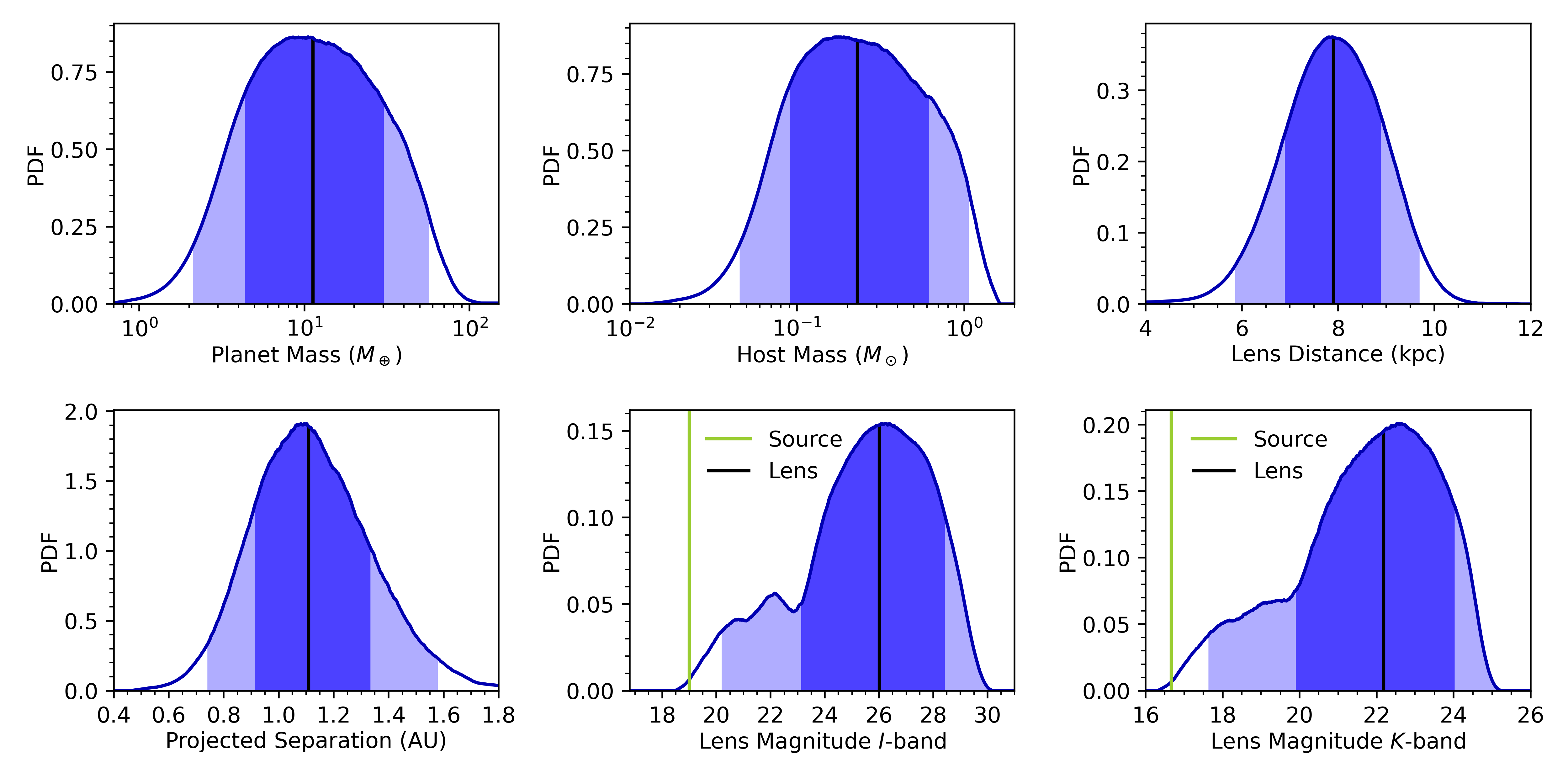
Figure 5: Lens system properties derived from the Bennett et al. (2014) Galactic model using a power-law stellar mass function with a prior uniform in $M$, $\mathop{}\!\mathrm{d}P\propto\mathop{}\!\mathrm{d}M$, meaning all stars have an equal planet-hosting probability. The 1$\sigma$ and 2$\sigma$ confidence intervals (i.e., $68.3\%$ and $95.5\%$) are represented by dark blue and median blue, respectively, with the median marked as a solid black line. For comparison, the source magnitude is shown as a green line in the lens magnitude graphs.

Usually, in microlensing papers, the estimations for the lens system properties assume that all the stars have equal probability of hosting a planet, which implies a mass function prior uniform in $M$. Statistical results on exoplanet populations were also obtained under the same assumption (Cassan et al., 2012). Yet, for this paper, we also consider a second scenario in which the probability of hosting a planet scales in proportion to the host star mass, $\mathop{}\!\mathrm{d}P\propto M\mathop{}\!\mathrm{d}M$. Johnson et al. (2007, 2010) found that, for their radial velocity sample, the planet occurrence increases with the stellar mass at fixed planet mass. This is compatible with Nielsen et al. (2019) direct imaging sample, which showed a strong correlation between planet occurrence rate and host star mass. Moreover, Bhattacharya et al. (2021) identified that the traditional assumption, which considers that all the stars have equal probability of hosting a planet, is not consistent with many microlensing events that have been revisited with the help of the Keck adaptive optics and had their lens object identified using high-angular resolution observations. Bhattacharya et al. (2021) pointed out that five of the six events with direct measurement of the separation between the source and the lens stars have found a host star more massive than the median predicted under the most conventional assumption, which is the one with a prior uniform in $M$. The authors also indicated that there is no publication bias for that Keck sample. Certainly, a more extensive sample to state this with more confidence is needed and, in fact, NASA Keck Key Strategic Mission Support and Hubble Space Telescope observing programs will be directly measuring the mass of more microlens host stars. Although planets are more likely to orbit around more massive stars, we still decide to consider both mass priors for our Bayesian assumptions, the conventional prior uniform in the stellar mass, and a prior that scales in proportion to the stellar mass.

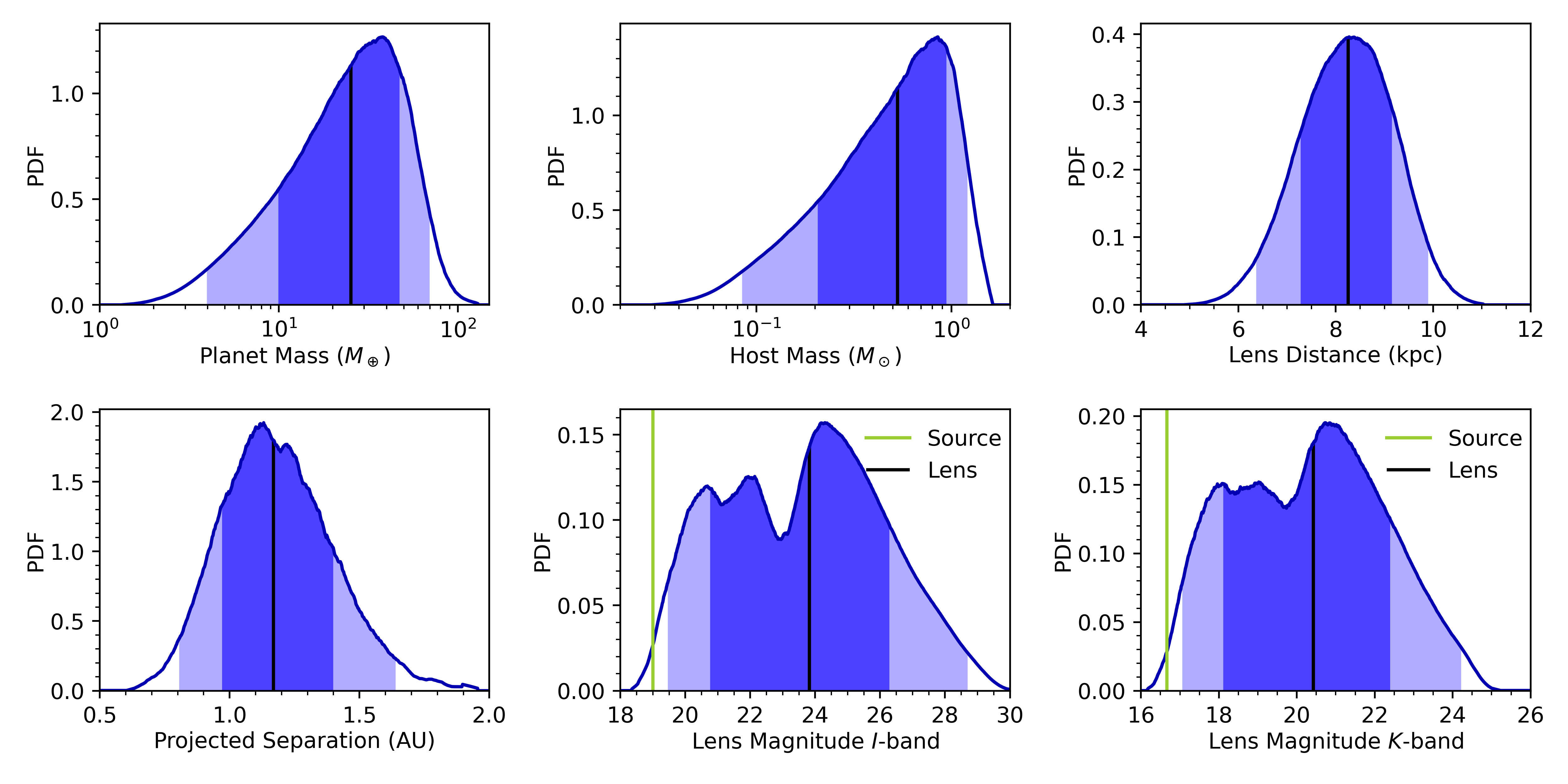
Figure 6: Lens system properties derived from the Bennett et al. (2014) Galactic model using a power-law stellar mass function under the assumption that the hosting probability scales in proportion to the stellar mass, $\mathop{}\!\mathrm{d}P\propto M\mathop{}\!\mathrm{d}M$. The 1$\sigma$ and 2$\sigma$ confidence intervals (i.e., $68.3\%$ and $95.5\%$) are represented by dark blue and median blue, respectively, with the median marked as a solid black line. For comparison, the source magnitude is shown as a green line in the lens magnitude graphs.

Results of the Bayesian analysis can also be affected when the probability of having a planet depends on the stellar location in our galaxy. However, it has recently been shown by Koshimoto et al. (2021) that the dependence of the planet-hosting probability on the Galactocentric distance is not large, thus we do not consider such dependence in this paper.

The Bayesian analysis for the lens properties is done using as input the collection of the MCMC runs (discussed in Section 3.1.2), with their fit parameters, along with our calculated angular source radius and extinction (see Section 4). To obtain the magnitude of the lens not only in the $I$-band, but also in the $K$-band, which is useful for future high-angular resolution follow-up observations, we use the extinction $A_{K}=0.2195$ (Gonzalez et al., 2012; Nishiyama et al., 2009). The Bennett et al. (2014) Galactic model is used two times, with the two different priors. First, we consider a power-law stellar mass function under the standard assumption that all stars have an equal planet-hosting probability, a function of the form $\mathop{}\!\mathrm{d}P\propto M^{\beta}\mathop{}\!\mathrm{d}M$ with $\beta=0$. Then we consider the same function but under the assumption that planets are more likely to orbit around more massive stars, so a function with $\beta=1$.

Under the assumption that the probability of hosting a planet is the same for all stars, $\beta=0\Rightarrow\mathop{}\!\mathrm{d}P\propto\mathop{}\!\mathrm{d}M$, we estimate that the lens physical properties and their $1\sigma$ ($68.3\%$) interval of confidence are $m_{\mathrm{planet}}=11.3_{-6.9}^{+19.2}\;M_{\oplus}$ for the planet mass, $M_{\mathrm{host}}=0.23_{-0.14}^{+0.39}\;M_{\odot}$ for the host mass, $D_{\mathrm{L}}=7.9_{-1.0}^{+1.0}\;\mathrm{kpc}$ for the distance to the lens, $a_{\perp}=1.11_{-0.20}^{+0.23}\;\mathrm{AU}$ for the project separation, $a_{\mathrm{3D}}=1.35_{-0.32}^{+0.75}\;\mathrm{AU}$ for the deprojected separation, and $I_{\mathrm{L}}=26.0_{-2.9}^{+2.4}$ and $K_{\mathrm{L}}=22.2_{-2.3}^{+1.9}$ for the lens magnitude. When assuming the mass function prior proportional to $M$, $\beta=1\Rightarrow\mathop{}\!\mathrm{d}P\propto M\mathop{}\!\mathrm{d}M$, the planet mass estimation is $m_{\mathrm{planet}}=25_{-15}^{+22}\;M_{\oplus}$, the host mass is $M_{\mathrm{host}}=0.53_{-0.32}^{+0.42}\;M_{\odot}$, the distance to the lens is $D_{\mathrm{L}}=8.3_{-1.0}^{+0.9}\;\mathrm{kpc}$, the projected separation is $a_{\perp}=1.17_{-0.20}^{+0.23}\;\mathrm{AU}$, the deprojected separation is $a_{\mathrm{3D}}=1.42_{-0.32}^{+0.78}\;\mathrm{AU}$, and lens magnitude is $I_{\mathrm{L}}=23.8_{-3.1}^{+2.5}$ and $K_{\mathrm{L}}=20.4_{-2.3}^{+2.0}$. We report the probability distributions considering both priors in Table 4.

Figure 5 shows the probability distribution of the planet and host masses, the distance to the lens system, their projected separation, and the lens magnitudes in both $I$-band and $K$-band, under the assumption of equal planet-hosting probability, $\mathop{}\!\mathrm{d}P\propto\mathop{}\!\mathrm{d}M$. Figure 6 shows the same results, but for the probability scaling in proportion to the host mass, $\mathop{}\!\mathrm{d}P\propto M\mathop{}\!\mathrm{d}M$. It is interesting to note that, even though the host mass and the planetary mass medians seem to be almost the double when comparing the results when the prior is uniform in $M$ to the results when the prior is proportional to $M$, the range for the masses are not that different when considering the $2\sigma$ (i.e., $95.5\%$) confidence interval.

6 Discussion

Our light-curve analysis for the event MOA-2020-BLG-135 leads to the discovery of MOA-2020-BLG-135Lb, a new Neptune-class planet. This analysis yields a planet-host mass ratio of $q=1.52_{-0.31}^{+0.39}\times 10^{-4}$, and separation $s\approx 1$. It is important to mention that with each MCMC chain we were able to sample all the modes of the posterior distribution due to the closeness of our close-separation ($s<1$) and wide-separation ($s>1$) solutions.

In Sections 4 and 5, we determine the source and the lens magnitude in K-band, aiming to anticipate results for high-angular resolution follow-up observations. The source magnitude with added extinction was computed to be $K_{\mathrm{S}}=16.67_{-0.25}^{+0.22}$. Under the assumption that all stars have equal planet-hosting probability, the lens magnitude is expected to be in the range $19.9-24.1$ for the $68.3\%$ ($1\sigma$) confidence interval, and $17.6-32.0$ for the $95.5\%$ ($2\sigma$) interval, with median $22.2$. One might wonder whether the lens star looks faint in comparison with the source star when considering only the median and the $1\sigma$ interval, which can indicate that its observation might be challenging in near future. However, for this assumption, when considering the $2\sigma$ interval of confidence, the result looks more encouraging. The event MOA-2007-BLG-400 had its lens object successfully identified using high-angular resolution observations, and the magnitude for the source and lens in Keck $K$-band were, respectively, $16.43\pm 0.04$ and $18.93\pm 0.08$ (Bhattacharya et al., 2021), which are not that different from our event, when considering the brightest possible lens magnitude. Moreover, on the assumption that the probability of hosting a planet scales in proportion to the stellar mass, the scenario gets even better, the lens magnitude is expected to be in the range $18.1-22.4$ for the $68.3\%$ ($1\sigma$) confidence interval, and $17.1-24.2$ for the $95.5\%$ ($2\sigma$) interval, with median $20.4$. Knowing that the microlensing events tend to have a host star more massive than their median predictions from only the light curve analysis, direct detection of the lens star looks promising for our event MOA-2020-BLG-135.

Another notable detail from our results is that a planet with a mass ratio $q=1.52_{-0.31}^{+0.39}\times 10^{-4}$ seems to be exactly where previous core accretion theories predicted a Neptune desert (Ida & Lin, 2004; Mordasini et al., 2009). On the other hand, it also lies exactly in the peak of the planet-to-star mass ratio distribution measured by gravitational microlensing (Suzuki et al., 2018). Once more, the Suzuki et al. (2016) contained only 30 planets and, to better understand this contradiction, we need a larger microlens exoplanet sample. The MOA collaboration has been working to obtain this extended sample, and will have more than 50 new planets, including the planet presented in this paper.

In Section 5, we discussed the Bayesian priors used for the analysis of the lens system properties subject to the microlensing light curve constraints. In almost all previous analyses with similar light curve constraints, it has been assumed that all host stars have an equal probability to host the planet with the measured mass ratio ($q=1.52_{-0.31}^{+0.39}\times 10^{-4}$ for this event). However, Bhattacharya et al. (2021) have shown that higher mass host stars appear to be more likely for the planets that the microlensing method is sensitive to. This is somewhat similar to earlier findings from radial velocity (Johnson et al., 2007, 2010) and direct detection (Nielsen et al., 2019) surveys. However, both of these analyses considered planet hosting probabilities at fixed planet mass instead of fixed mass ratio. Since lower mass ratio planets are more common (Suzuki et al., 2016), for mass ratios $\geq 10^{-4}$, the demonstration that higher mass hosts are more likely for a fixed mass ratio is stronger than the same claim at fixed planet mass. If the planet hosting probability was independent of host mass at fixed mass ratio, the hosting probability would be higher for higher mass hosts at fixed planet mass, since this implies a larger mass ratio, $q$, for the lower mass hosts (as long as $\geq 10^{-4}$).

7 Conclusion

We have presented the discovery of MOA-2020-BLG-135Lb, a new Neptune-class planet uncovered by the light-curve analysis for the microlensing event MOA-2020-BLG-135. By applying the Bennett (2010) process, our analysis has revealed a planet-host mass ratio of $q=1.52_{-0.31}^{+0.39}\times 10^{-4}$, and separation $s\approx 1$.

To estimate the lens system properties for MOA-2020-BLG-135, we have conducted a Bayesian analysis using the Bennett et al. (2014) Galactic model. When considering that all stars have equal probability of hosting a planet, using a mass function prior uniform in $M$, we have found a planet mass of $m_{\mathrm{planet}}=11.3_{-6.9}^{+19.2}\;M_{\oplus}$, a host-star with mass of $M_{\mathrm{host}}=0.23_{-0.14}^{+0.39}\;M_{\odot}$ and magnitude $K_{\mathrm{L}}=22.2_{-2.3}^{+1.9}$, located at a distance $D_{\mathrm{L}}=7.9_{-1.0}^{+1.0}\;\mathrm{kpc}$. Under the assumption that the hosting-probability scales in proportion to the stellar mass, we have estimated $m_{\mathrm{planet}}=25_{-15}^{+22}\;M_{\oplus}$, $M_{\mathrm{host}}=0.53_{-0.32}^{+0.42}\;M_{\odot}$, $K_{\mathrm{L}}=20.4_{-2.3}^{+2.0}$, and $D_{\mathrm{L}}=8.3_{-1.0}^{+0.9}\;\mathrm{kpc}$.

The previous results from RV and direct imaging (Johnson et al., 2007, 2010; Nielsen et al., 2019) considered planet hosting probabilities for fixed planet mass, whereas the MOA-II exoplanet microlens statistical analysis considers mass ratio. MOA-2020-BLG-135Lb is an important detection for completeness of the extended MOA-II exoplanet microlens statistical sample. Additionally, high-angular resolution follow-up observations for this event are certainly recommended in the future for restricting the mass values of the host star and its planet.

References

- Alard (2000) Alard, C. 2000, Astronomy and Astrophysics Supplement Series, 144, 363
- Alard & Lupton (1998) Alard, C., & Lupton, R. H. 1998, The Astrophysical Journal, 503, 325
- Ali-Dib et al. (2022) Ali-Dib, M., Cumming, A., & Lin, D. N. 2022, Monthly Notices of the Royal Astronomical Society, 509, 1413
- An (2021) An, J. 2021, arXiv preprint arXiv:2102.07950
- Batista (2018) Batista, V. 2018, Handbook of Exoplanets, 120
- Bennett (2008) Bennett, D. 2008, Exoplanets ed J. Mason, Berlin: Springer
- Bennett et al. (2012) Bennett, D., Sumi, T., Bond, I., et al. 2012, The Astrophysical Journal, 757, 119
- Bennett et al. (2017) Bennett, D., Bond, I., Abe, F., et al. 2017, The Astronomical Journal, 154, 68
- Bennett et al. (2018) Bennett, D., Udalski, A., Han, C., et al. 2018, The Astronomical Journal, 155, 141
- Bennett (2010) Bennett, D. P. 2010, The Astrophysical Journal, 716, 1408
- Bennett & Rhie (1996) Bennett, D. P., & Rhie, S. H. 1996, The Astrophysical Journal, 472, 660
- Bennett et al. (2014) Bennett, D. P., Batista, V., Bond, I., et al. 2014, The Astrophysical Journal, 785, 155
- Bensby et al. (2011) Bensby, T., Adén, D., Melendez, J., et al. 2011, Astronomy & Astrophysics, 533, A134
- Bhattacharya et al. (2021) Bhattacharya, A., Bennett, D. P., Beaulieu, J. P., et al. 2021, The Astronomical Journal, 162, 60
- Bond et al. (2001) Bond, I., Abe, F., Dodd, R., et al. 2001, Monthly Notices of the Royal Astronomical Society, 327, 868
- Bond et al. (2004) Bond, I. A., Udalski, A., Jaroszyński, M., et al. 2004, The Astrophysical Journal Letters, 606, L155
- Bond et al. (2017) Bond, I. A., Bennett, D. P., Sumi, T., et al. 2017, MNRAS, 469, 2434, doi: 10.1093/mnras/stx1049
- Boyajian et al. (2014) Boyajian, T. S., Van Belle, G., & Von Braun, K. 2014, The Astronomical Journal, 147, 47
- Cassan et al. (2012) Cassan, A., Kubas, D., Beaulieu, J. P., et al. 2012, Nature, 481, 167, doi: 10.1038/nature10684
- Dominik (1999) Dominik, M. 1999, arXiv preprint astro-ph/9903014
- Fukugita et al. (1996) Fukugita, M., Ichikawa, T., Gunn, J., et al. 1996, The Astronomical Journal, 111, 1748
- Gaudi (2012) Gaudi, B. S. 2012, Annual Review of Astronomy and Astrophysics, 50, 411
- Gonzalez et al. (2012) Gonzalez, O., Rejkuba, M., Zoccali, M., et al. 2012, Astronomy & Astrophysics, 543, A13
- Gould et al. (2010) Gould, A., Dong, S., Bennett, D. P., et al. 2010, The Astrophysical Journal, 710, 1800
- Gould & Loeb (1992) Gould, A., & Loeb, A. 1992, The Astrophysical Journal, 396, 104
- Griest & Safizadeh (1998) Griest, K., & Safizadeh, N. 1998, The Astrophysical Journal, 500, 37
- Guerrero et al. (2021) Guerrero, N. M., Seager, S., Huang, C. X., et al. 2021, The Astrophysical Journal Supplement Series, 254, 39
- Holtzman et al. (1998) Holtzman, J. A., Watson, A. M., Baum, W. A., et al. 1998, The Astronomical Journal, 115, 1946
- Hunter (2007) Hunter, J. D. 2007, CSE, 9, 90, doi: 10.1109/MCSE.2007.55
- Ida & Lin (2004) Ida, S., & Lin, D. N. 2004, The Astrophysical Journal, 604, 388
- Johnson et al. (2010) Johnson, J. A., Aller, K. M., Howard, A. W., & Crepp, J. R. 2010, Publications of the Astronomical Society of the Pacific, 122, 905
- Johnson et al. (2007) Johnson, J. A., Butler, R. P., Marcy, G. W., et al. 2007, The Astrophysical Journal, 670, 833
- Jones et al. (2001) Jones, E., Oliphant, T., Peterson, P., et al. 2001, SciPy: Open source scientific tools for Python. http://www.scipy.org/
- Kenyon & Hartmann (1995) Kenyon, S. J., & Hartmann, L. 1995, The Astrophysical Journal Supplement Series, 101, 117
- Kim et al. (2016) Kim, S.-L., Lee, C.-U., Park, B.-G., et al. 2016, Journal of the Korean Astronomical Society, 49, 37
- Koshimoto et al. (2021) Koshimoto, N., Bennett, D. P., Suzuki, D., & Bond, I. A. 2021, The Astrophysical Journal Letters, 918, L8
- Mao & Paczynski (1991) Mao, S., & Paczynski, B. 1991, The Astrophysical Journal, 374, L37
- Metropolis et al. (1953) Metropolis, N., Rosenbluth, A. W., Rosenbluth, M. N., Teller, A. H., & Teller, E. 1953, The journal of chemical physics, 21, 1087
- Mordasini et al. (2009) Mordasini, C., Alibert, Y., & Benz, W. 2009, Astronomy & Astrophysics, 501, 1139
- Nataf et al. (2013) Nataf, D. M., Gould, A., Fouqué, P., et al. 2013, The Astrophysical Journal, 769, 88
- Nielsen et al. (2019) Nielsen, E. L., De Rosa, R. J., Macintosh, B., et al. 2019, The Astronomical Journal, 158, 13
- Nishiyama et al. (2009) Nishiyama, S., Tamura, M., Hatano, H., et al. 2009, The Astrophysical Journal, 696, 1407
- Oliphant (2015) Oliphant, T. E. 2015, Guide to NumPy (2nd ed.; CreateSpace). https://www.xarg.org/ref/a/151730007X/
- Paczynski (1986) Paczynski, B. 1986, The Astrophysical Journal, 304, 1
- Ranc (2020) Ranc, C. 2020, Microlensing Observations ANAlysis tools, Zenodo, doi: 10.5281/zenodo.4257008
- Schwarz (1978) Schwarz, G. 1978, The annals of statistics, 461
- Sumi et al. (2013) Sumi, T., Bennett, D., Bond, I., et al. 2013, The Astrophysical Journal, 778, 150
- Suzuki et al. (2016) Suzuki, D., Bennett, D., Sumi, T., et al. 2016, The Astrophysical Journal, 833, 145
- Suzuki et al. (2018) Suzuki, D., Bennett, D. P., Ida, S., et al. 2018, The Astrophysical Journal Letters, 869, L34
- Szymański et al. (2011) Szymański, M., Udalski, A., Soszyński, I., et al. 2011, arXiv preprint arXiv:1107.4008
- Tomaney & Crotts (1996) Tomaney, A. B., & Crotts, A. P. 1996, arXiv preprint astro-ph/9610066
- Van Belle (1999) Van Belle, G. T. 1999, Publications of the Astronomical Society of the Pacific, 111, 1515
- Yee et al. (2021) Yee, J. C., Zang, W., Udalski, A., et al. 2021, The Astronomical Journal, 162, 180
- Yoo et al. (2004) Yoo, J., DePoy, D., Gal-Yam, A., et al. 2004, The Astrophysical Journal, 603, 139
- Zang et al. (2018) Zang, W., Penny, M. T., Zhu, W., et al. 2018, Publications of the Astronomical Society of the Pacific, 130, 104401
- Zang et al. (2021) Zang, W., Han, C., Kondo, I., et al. 2021, Research in Astronomy and Astrophysics, 21, 239