Embedding of Functional Human Brain Networks on a Sphere

Abstract

Human brain activity is often measured using the blood-oxygen-level dependent (BOLD) signals obtained through functional magnetic resonance imaging (fMRI). The strength of connectivity between brain regions is then measured as a Pearson correlation matrix. As the number of brain regions increases, the dimension of matrix increases. It becomes extremely cumbersome to even visualize and quantify such weighted complete networks. To remedy the problem, we propose to embed brain networks onto a sphere, which is a Riemannian manifold with constant positive curvature. The Matlab code for the spherical embedding is given in https://github.com/laplcebeltrami/sphericalMDS.

1 Introduction

In functional magnetic resonance imaging (fMRI) studies of human brain, brain activity is measured by the blood-oxygen-level dependent (BOLD) contrast. This can be used to map neural activity in the brain. The strength of neural connectivity between regions is then measured using the Pearson correlation (Figure 1) [7]. The whole brain is often parcellated into $p$ disjoint regions, where $p$ is usually a few hundreds [3, 15]. Subsequently, either functional or structural information is overlaid on top of the parcellation and $p\times p$ connectivity matrix $C=(c_{ij})$ that measures the strength of connectivity between brain regions $i$ and $j$ is obtained. Recently, we are beginning to see large-scale brain networks that are more effective in localizing regions and increasing prediction power [4, 34]. However, increasing parcellation resolution also increases the computational burden exponentially.

For an undirected network with $p$ number of nodes, there are $p(p-1)/2$ number of edges and thus, the brain network is considered as an object in dimension $p(p-1)/2$. Such high dimensional data often requires $\mathcal{O}(p^{3})$ run time for various matrix manipulations such as matrix inversion and singular value decomposition (SVD). Even at 3mm resolution, fMRI has more than 25000 voxels in the brain [4]. It requires about 5GB of storage to store the matrix of size $25000\times 25000$ (Figure 1). At 1mm resolution, there are more than 300000 voxels and it requires more than 670GB of storage. Considering large-scale brain imaging datasets such has HCP (Human Connetome Project http://www.humanconnectomeproject.org) often have thousands images, various learning and inference at higher spatial resolution would be a serious computational and storage challenge. We directly address these challenges by embedding the brain networks into 3D unit sphere. Although there are few available technique for embedding graphs into hyperbolic spaces, the hyperbolic spaces are not intuitive and not necessarily easier to compute [27, 31]. Since numerous computational tools have been developed for spherical data, we propose to embed brain networks on a 3D sphere and utilizes such tools. The spherical network embedding will offer far more adaptability and applicability in various problems.

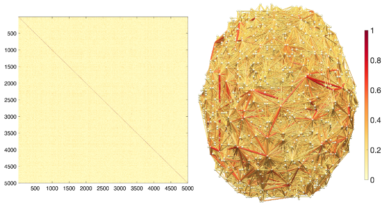
Figure 1: The correlation brain network (left) obtained from the resting-state functional magnetic resonance images (rs-fMRI) of a healthy subject at 5000 regions [4, 17]. The network is so dense to visualize all the edges (right), only the connections with positive correlations are shown. Beyond visualization, performing various matrix and graph operations on such a dense network is computationally time consuming and often not feasible.

2 Embedding onto a sphere

Consider a weighted complete graph $G=(V,C)$ consisting of node set $V=\left\{1,\dots,p\right\}$ and edge weight $C=(c_{ij})$, where $c_{ij}$ is the weight between nodes $i$ and $j$. The edge weights in most brain networks are usually given by some sort of similarity measure between nodes [23, 24, 26, 28, 33]. Most often the Pearson correlation is used in brain network modeling [7] (Figure 1).

Suppose measurement vector ${\bf x}_{j}=(x_{1j},\cdots,$ $x_{nj})^{\top}\in\mathbb{R}^{n}$ is given on node $j$ over $n$ variables or subjects. We center and rescale the measurement ${\bf x}_{j}$ such that

$${\bf x}_{j}^{\top}{\bf x}_{j}=\sum_{i=1}^{n}x_{ij}^{2}=1,\quad\sum_{i=1}^{n}x_{ij}=0.$$

We can show that $c_{ij}={\bf x}_{i}^{\top}{\bf x}_{j}$ is the Pearson correlation [7]. Such points are in the $n$-dimensional sphere $S^{n-1}$. Let the $n\times p$ data matrix be ${\bf X}=[{\bf x}_{1},\cdots,{\bf x}_{p}].$ Then the correlation matrix is given by ${\bf X}^{\top}{\bf X}$

$${\bf X}^{\top}{\bf X}=({\bf x}_{i}^{\top}{\bf x}_{j})=U^{\top}D(\eta_{1},\cdots,\eta_{p})U$$ (1)

with $U^{\top}U=I_{p}$ and $D$ is a diagonal matrix with eigenvalues $\eta_{1}\geq\cdots\geq\eta_{p}$. Since there are usually more nodes than variables in brain images, i.e., $n\ll p$, the correlation matrix is not positive definite and some eigenvalues might be zeros [4]. Since the correlation is a similarity measure, it is not distance. Often used correlation distance $c_{ij}=1-{\bf x}_{i}^{\top}{\bf x}_{j}$ is not metric. To see this, consider the following 3-node counter example:

$${\bf x}_{1}=(0,\frac{1}{\sqrt{2}},-\frac{1}{\sqrt{2}})^{\top},\quad{\bf x}_{2}=(\frac{1}{\sqrt{2}},0,-\frac{1}{\sqrt{2}})^{\top},\quad{\bf x}_{3} = (\frac{1}{\sqrt{6}},\frac{1}{\sqrt{6}},-\frac{2}{\sqrt{6}})^{\top}.$$

Then we have $c_{12}>c_{13}+c_{23}$ disproving triangle inequality. Then the question is under what condition, the Pearson correlations becomes a metric?

Theorem 2.1.

For centered and scaled data ${\bf x}_{1},\cdots,{\bf x}_{p}$, $\theta_{ij}=cos^{-1}({\bf x}_{i}^{\top}{\bf x}_{j})$ is a metric.

Proof. The centered and scaled data ${\bf x}_{i}$ and ${\bf x}_{j}$ are residing on the unit sphere $S^{n-1}$. The correlation between ${\bf x}_{i}$ and ${\bf x}_{j}$ is the cosine angle $\theta_{ij}$ between the two vectors, i.e.,

$${\bf x}_{i}^{\top}{\bf x}_{j}=\cos\theta_{ij}.$$

The geodesic distance $d$ between nodes ${\bf x}_{i}$ and ${\bf x}_{j}$ on the unit sphere is given by angle $\theta_{ij}$:

$$\theta_{ij}=\cos^{-1}({\bf x}_{i}^{\top}{\bf x}_{j}).$$

For nodes ${\bf x}_{i},{\bf x}_{j}\in S^{n-1}$, there are two possible angles $\theta_{ij}$ and $2\pi-\theta_{ij}$ depending on if we measure the angle along the shortest or longest arcs. We take the convention of using the smallest angle in defining $\theta_{ij}$. With this convention,

$$\theta_{ij}\leq\pi.$$

Given three nodes ${\bf x}_{i},{\bf x}_{j}$ and ${\bf x}_{k}$, which forms a spherical triangle, we then have spherical triangle inequality

$$\theta_{ij}\leq\theta_{ik}+\theta_{kj}.$$ (2)

The inequality (2) is proved in [29]. Other conditions for metric are trivial. ∎

Theorem 2.1 shows that measurement vector ${\bf x}_{j}$ can be embedded onto a sphere $S^{n-1}$ without any loss of information. The geodesic $d({\bf x}_{i},{\bf x}_{j})$ on the sphere is the Pearson correlation. A similar approach is proposed for embedding an arbitrary distance matrix to a sphere in [36]. In our case, the problem is further simplified due to the geometric structure of correlation matrices [7].

3 Hypersperical harmonic expansion of brain networks

Once we embedded correlation networks onto a sphere, it is possible to algebraically represent such networks as basis expansion involving the hyperspherical harmonics [11, 19, 20, 21, 22]. Let $\boldsymbol{\varphi}=(\theta,\varphi_{2},\cdots,\varphi_{n-1})$ be the spherical coordinates of $S^{n-1}$ such that $\theta\in[0,\pi),\varphi_{i}\in[0,2\pi)$ where $\theta$ is the axial angle. Then the spherical Laplacian $\Delta_{n-1}$ is iteratively given as [8]

$$\Delta_{n-1}=\frac{\partial^{2}}{\partial\theta^{2}}+(n-2)\cot\theta\frac{\partial}{\partial\theta}+\frac{1}{\sin^{2}\theta}\Delta_{n-2}.$$

With respect to the spherical Laplacian $\Delta_{n-1}$, the hyperspherical harmonics $Y_{\bf l}(\boldsymbol{\varphi})$ with ${\bf l}=(l_{1},\cdots,l_{n-1})$ satisfies

$$\Delta_{n-1}Y_{\bf l}(\boldsymbol{\varphi})=-\lambda_{\bf l}Y_{\bf l}(\boldsymbol{\varphi})$$

with eigenvalues $\lambda_{\bf l}=l_{n-1}(l_{n-1}+n-1)$ for $|l_{1}|\leq l_{2}\leq\cdots l_{n-1}$. The hyperspherical harmonics are given in terms of the Legendre polynomials. We can compute the hyperspherical harmonics inductively from the previous dimension starting with $S^{2}$, which we parameterize with $(\theta,\varphi_{2})\in[0,\pi)\otimes[0,2\pi)$, where the spherical harmonics $Y_{l_{2}l_{1}}$ are given by [6, 9]

$$Y_{l_{2}l_{1}}=\begin{cases}c_{l_{2}l_{1}}P^{|l_{1}|}_{l_{2}}(\cos\theta)\sin(|l_{1}|\varphi_{2}),&-l_{2}\leq l_{1}\leq-1,\\ \frac{c_{l_{2}l_{1}}}{\sqrt{2}}P_{l_{2}}^{|l_{1}|}(\cos\theta),&L_{1}=0,\\ c_{l_{2}l_{1}}P^{|l_{1}|}_{l_{2}}(\cos\theta)\cos(|l_{1}|\varphi_{2}),&1\leq l_{1}\leq l_{2},\end{cases}$$

with normalizing constants $c_{l_{2}l_{1}}$ and the associated Legendre polynomial $P_{l_{2}}^{l_{1}}(x)$ [6].

The hyperspherical harmonics are orthonormal with respect to area element

$$d\mu(\boldsymbol{\varphi})=\sin^{n-2}\theta\sin^{n-3}\varphi_{2}\cdots\sin\varphi_{n-1}d\boldsymbol{\varphi}$$

such that

$$\langle Y_{{\bf l}_{1}}Y_{{\bf l}_{2}}\rangle = \int_{S^{n-1}}Y_{{\bf l}_{1}}(\boldsymbol{\varphi})Y_{{\bf l}_{2}}(\boldsymbol{\varphi})\;d\mu(\boldsymbol{\varphi})=\delta_{{\bf 1}_{1}{\bf 1}_{2}},$$

where $\delta_{{\bf 1}_{1}{\bf 1}_{2}}$ is the Kronecker’s delta. Then using the hyperspherical harmonics, we can build the multiscale representation of networks through the heat kernel expansion [5, 6]

$$K_{t}(\boldsymbol{\varphi},\boldsymbol{\varphi}^{\prime})=\sum_{\bf l}e^{-\lambda_{\bf l}t}Y_{\bf l}(\boldsymbol{\varphi})Y_{\bf l}(\boldsymbol{\varphi}^{\prime}),$$

where the summation is over all possible valid integer values of ${\bf l}$.

Given initial data $g(t=0,\boldsymbol{\varphi})=f(\boldsymbol{\varphi})$ on $S^{n-1}$, the solution to diffusion equation

$$\frac{dg}{dt}=\Delta_{n-1}g$$

at time $t$ is given by

$$g(t,\boldsymbol{\varphi}) = \int_{S^{n-1}}K_{t}(\boldsymbol{\varphi},\boldsymbol{\varphi}^{\prime})f(\boldsymbol{\varphi}^{\prime})\;d\mu(\boldsymbol{\varphi}^{\prime})$$

$$= \sum_{{\bf l}}e^{-\lambda_{\bf l}t}f_{\bf l}Y_{\bf l}(\boldsymbol{\varphi})$$

with spherical harmonic coefficients $f_{\bf l}=\langle f,Y_{\bf l}\rangle$. The coefficients are often estimated in the least squares fashion in the spherical harmonic representation (SPHARM) often used in brain cortical shape modeling (https://github.com/laplcebeltrami/weighted-SPHARM) [6, 14, 18, 30]. The embedded network nodes can be modeled as the Dirac delta function such that

$$f(\boldsymbol{\varphi})=\frac{1}{p}\sum_{i=1}^{p}\delta(\boldsymbol{\varphi}-{\bf x}_{i}).$$

We normalize the expression such that $\int_{S^{n-1}}f(\boldsymbol{\varphi})d\mu(\boldsymbol{\varphi})=1.$ Then we can algebraically show that the solution is given by

$$g(t,\boldsymbol{\varphi})=\sum_{{\bf l}}e^{-\lambda_{\bf l}t}Y_{\bf l}(\boldsymbol{\varphi})\sum_{i=1}^{p}Y_{\bf l}({\bf x}_{i}).$$

4 Spherical multidimensional scaling

We have shown how to embed correlation matrices into $S^{n-1}$ and model them parametrically using the spherical harmonics. In many large scale brain imaging studies, the number of variables $n$ can be thousands. Embedding in such a high dimensional sphere may not be so useful in practice. We propose to embed correlation matrices into two sphere $S^{2}$, which is much easier to visualize and provides parametric representation through available SPAHRM tools [5].

Given geodesic $\theta_{ij}=\cos^{-1}({\bf x}_{i}^{\top}{\bf x}_{j})$ in $S^{n-1}$, we want to find the lower dimensional embedding ${\bf y}_{j}=(y_{1j},y_{2j},y_{3j})^{\top}\in S^{2}$ satisfying

$$\|{\bf y}_{j}\|^{2}={\bf y}_{j}^{\top}{\bf y}_{j}=\sum_{i=1}^{3}y_{ij}^{2}=1.$$

This is a spherical multidimensional scaling (MDS) often encountered in analyzing spherical data such as earthquakes [12] and colors in computer vision [25]. Given data matrix ${\bf X}$ in (1), we find ${\bf Y}=[{\bf y}_{1},\cdots,{\bf y}_{p}]$ that minimizes the loss

$$\mathcal{L}({\bf X},{\bf Y})=\sum_{i,j=1}^{p}\big{[}\cos^{-1}({\bf x}_{i}^{\top}{\bf x}_{j})-\cos^{-1}({\bf y}_{i}^{\top}{\bf y}_{j})\big{]}^{2}.$$ (3)

We propose to solve spherical MDS (3) without the usual gradient descent on spherical coordinates [25]. At the minimum of (3), we can approximate the loss linearly using the Taylor expansion [1]

$$\cos^{-1}({\bf x}_{i}^{\top}{\bf x}_{j})=\frac{\pi}{2}-{\bf x}_{i}^{\top}{\bf x}_{j}+\cdots$$

as

$$\mathcal{L}({\bf X},{\bf Y})=\sum_{i,j=1}^{p}\big{[}{\bf x}_{i}^{\top}{\bf x}_{j}-{\bf y}_{i}^{\top}{\bf y}_{j}\big{]}^{2}.$$ (4)

The loss (4) can be further written in the matrix form

$$\mathcal{L}({\bf X},{\bf Y})=\mbox{tr}({\bf X}^{\top}{\bf X}-{\bf Y}^{\top}{\bf Y})^{2}=\|{\bf X}^{\top}{\bf X}-{\bf Y}^{\top}{\bf Y}\|_{F}^{2},$$ (5)

with the Frobenius norm $\|\cdot\|_{F}$. The minimization of linearized loss (5) is a low-rank approximation problem, which can be solved exactly through the Eckart Young Mirsky theorem [16] that states

$$\arg\min_{{\bf Y}^{\top}{\bf Y}}\mathcal{L}({\bf X},{\bf Y})=U^{\top}D(\eta_{1},\eta_{2},\eta_{3},0,\cdots,0)U,$$

where $U$ is the orthogonal matrix obtained as the SVD of ${\bf X}^{\top}{\bf X}$ in (1) [10]. In order to match two given symmetric matrices, we need to align with the principle directions of the the matrices. The matching is then the most optimal in the Frobenius norm sense. However, the result of the Eckart Young Mirsky theorem does not constrain and and embeded points ${\bf Y}=[{\bf y}_{1},\cdots,{\bf y}_{p}]$ are not necessary constrained on the sphere. Thus, we need to normalize ${\bf Y}$ such that ${\bf y}_{j}\in S^{2}$ as follows.

Let $[{\bf v}_{1},\cdots,{\bf v}_{p}]$ be $3\times p$ matrix consisting of the first three rows of $D(\sqrt{\eta_{1}},\sqrt{\eta_{2}},\\ \sqrt{\eta_{3}},0,\cdots,0)U$. All other rows below are zero. Then each column vector ${\bf v}_{j}$ is normalized to be embededed on the unit sphere such that $\frac{{\bf v}_{j}}{\|{\bf v}_{j}\|}\in S^{2}$. Since

$$\Big{(}\frac{{\bf v}_{i}^{\top}{\bf v}_{j}}{\|{\bf v}_{i}\|\|{\bf v}_{j}\|}\Big{)}=U^{\top}D(\eta_{1},\eta_{2},\eta_{3},0,\cdots,0)U,$$

${\bf Y}=\Big{[}\frac{{\bf v}_{1}}{\|{\bf v}_{1}\|},\cdots,\frac{{\bf v}_{p}}{\|{\bf v}_{p}\|}\Big{]}$ solves (5) and we claim

Theorem 4.1.

$$\arg\min_{{\bf y}_{j}\in S^{2}}\mathcal{L}({\bf X},{\bf Y})=\Big{[}\frac{{\bf v}_{1}}{\|{\bf v}_{1}\|},\cdots,\frac{{\bf v}_{p}}{\|{\bf v}_{p}\|}\Big{]}.$$

The embedding is not unique. For any rotation matrix $Q$, $Q{\bf Y}$ will be another embedding. In brain imaging applications, where we need to embed multiple brain networks, the rotation matrix $Q$ should not come from individual subject but should come from the fixed average template.

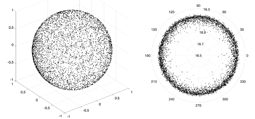
Figure 2: Left: embedding of a brain network with 5000 nodes to sphere $S^{2}$. Each scatter point can be modeled as the Dirac delta function. Right: embedding to hyperbolic space, where the embedded points from a torus-like circular pattern.

5 Experiement

We applied the proposed spherical embedding to a functional brain network obtained through the Human Connectome Project (HCP) [32, 35]. The resting-state functional magnetic resonance image (rs-fMRI) of a healthy subject was collected with 3T scanner at 2.0 mm voxel resolution (91×109×91 spatial dimensionality), 1200 frames at a rate of one frame every 720 ms. The scan went through spatial and temporal preprocessing including spatial distortions and motion correction, frequency filtering, artifact removal as the part of HCP preprocessing pipeline [32]. fMRI is then denoised using the Fourier series expansion with cosine basis [17]. A correlation matrix of size 5000 $\times$ 5000 was obtained by computing the Pearson correlation of the expansion coefficients across uniformly sampled 5000 brain regions (Figure 1). Following the proposed method, we embedded the brain network into 5000 scatter points on $S^{2}$ (Figure 2). The method seems to embed brain networks uniformly across $S^{2}$. The Shepard diagram of displaying distance $\cos^{-1}({\bf y}_{i}^{\top}{\bf y}_{j})$ vs. $\cos^{-1}({\bf x}_{i}^{\top}{\bf x}_{j})$ is given in Figure 3. The correlation between the distances is 0.51 indicating a reasonable embedding performance. The Matlab code for performing the spherical embedding is provided in https://github.com/laplcebeltrami/sphericalMDS.

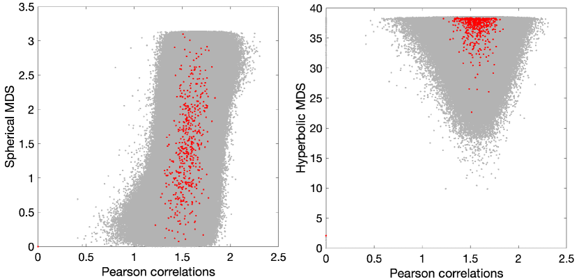
Figure 3: The shepard diagrams of all the pairwise distances (gray points) on 5000 nodes with spherical MDS (left) and hyperbolic MDS. Red points are first 500 pairwise distances. The geodesic distance $\cos^{-1}({\bf x}_{i}^{\top}{\bf x}_{j})$ is used for Pearson correlations. The correlation between distances are 0.51 for spherical MDS and 0.0501 for hyperbolic MDS demonstrating far better embedding performance of spherical MDS.

6 Discussion

The embedding of brain networks to a sphere allows various computation of brain networks straightforward. Instead of estimating the network gradient discretely in coarse fashion, it is possible to more smoothly estimate the network gradient on a sphere using the spherical coordinates [13]. We can further able to obtain various differential quantities of brain networks such as gradient and curls often used in the Hodge decomposition [2]. This is left as a future study.

The major body of literature on the embedding of networks is toward hyperbolic spaces, where 2D Poincare disk $D$ is often used [27, 31, 36]. Figure 2 shows the embedding of the brain network to $D$ using hyperbolic MSD [37]. It is usually characterized by the torus-like circular pattern. Unlike spherical embedding, the hyperbolic embedding does not provide uniform scatter points.

The Shepard diagram of displaying the geodesic distance in the Poincare disk vs. $\cos^{-1}({\bf x}_{i}^{\top}{\bf x}_{j})$ is given in Figure 3. The correlation between distances is 0.0501 indicating a poor embedding performance compared to the spherical MDS. For correlation based brain networks, the spherical MDS might be a better alternative over hyperbolic MDS. However, further investigation is needed for determining the optimal embedding method for brain networks.

References

- [1] M. Abramowitz, I.A. Stegun, and R.H. Romer. Handbook of mathematical functions with formulas, graphs, and mathematical tables. American Association of Physics Teachers, 1988.
- [2] D.V. Anand, , S. Dakurah, B. Wang, and M.K. Chung. Hodge-Laplacian of brain networks and its application to modeling cycles. arXiv preprint arXiv:2110.14599, 2021.
- [3] S. Arslan, S.I. Ktena, A. Makropoulos, E.C. Robinson, D. Rueckert, and S. Parisot. Human brain mapping: A systematic comparison of parcellation methods for the human cerebral cortex. NeuroImage, 170:5–30, 2018.
- [4] M.K. Chung. Statistical challenges of big brain network data. Statistics and Probability Letter, 136:78–82, 2018.
- [5] M.K. Chung, K.M. Dalton, and R.J. Davidson. Tensor-based cortical surface morphometry via weighted spherical harmonic representation. IEEE Transactions on Medical Imaging, 27:1143–1151, 2008.
- [6] M.K. Chung, R. Hartley, K.M. Dalton, and R.J. Davidson. Encoding cortical surface by spherical harmonics. Statistica Sinica, 18:1269–1291, 2008.
- [7] M.K. Chung, H. Lee, A. DiChristofano, H. Ombao, and V. Solo. Exact topological inference of the resting-state brain networks in twins. Network Neuroscience, 3:674–694, 2019.
- [8] H.S. Cohl. Opposite antipodal fundamental solution of Laplace’s equation in hyperspherical geometry. SIGMA. Symmetry, Integrability and Geometry: Methods and Applications, 7:108, 2011.
- [9] R. Courant and D. Hilbert. Methods of Mathematical Physics. Interscience, New York, English edition, 1953.
- [10] A. Dax. Low-rank positive approximants of symmetric matrices. Advances in Linear Algebra & Matrix Theory, 4:172, 2014.
- [11] G. Domokos. Four-dimensional symmetry. Physical Review, 159:1387–1403, 1967.
- [12] W. Dzwinel, D.A. Yuen, K. Boryczko, Y. Ben-Zion, S. Yoshioka, and T. Ito. Nonlinear multidimensional scaling and visualization of earthquake clusters over space, time and feature space. Nonlinear Processes in Geophysics, 12:117–128, 2005.
- [13] A. Elad, Y. Keller, and R. Kimmel. Texture mapping via spherical multi-dimensional scaling. In International Conference on Scale-Space Theories in Computer Vision, pages 443–455. Springer, 2005.
- [14] G. Gerig, M. Styner, D. Jones, D. Weinberger, and J. Lieberman. Shape analysis of brain ventricles using SPHARM. In MMBIA, pages 171–178, 2001.
- [15] M.F. Glasser, S.M. Smith, D.S. Marcus, J.L.R. Andersson, E.J. Auerbach, T.E.J. Behrens, T.S. Coalson, M.P. Harms, M. Jenkinson, and S. Moeller. The human connectome project’s neuroimaging approach. Nature Neuroscience, 19:1175, 2016.
- [16] Gene H Golub, Alan Hoffman, and Gilbert W Stewart. A generalization of the Eckart-Young-Mirsky matrix approximation theorem. Linear Algebra and its applications, 88:317–327, 1987.
- [17] A. Gritsenko, M. Lindquist, and M.K. Chung. Twin classification in resting-state brain connectivity. In 2020 IEEE 17th International Symposium on Biomedical Imaging (ISBI), pages 1391–1394, 2020.
- [18] X. Gu, Y.L. Wang, T.F. Chan, T.M. Thompson, and S.T. Yau. Genus zero surface conformal mapping and its application to brain surface mapping. IEEE Transactions on Medical Imaging, 23:1–10, 2004.
- [19] A. Higuchi. Symmetric tensor spherical harmonics on the N-sphere and their application to the de sitter group SO(N, 1). Journal of mathematical physics, 28:1553–1566, 1987.
- [20] A.P. Hosseinbor, M.K. Chung, C.G. Koay, S.M. Schaefer, C.M. Van Reekum, L.P. Schmitz, M. Sutterer, A.L. Alexander, and R.J. Davidson. 4D hyperspherical harmonic (HyperSPHARM) representation of surface anatomy: A holistic treatment of multiple disconnected anatomical structures. Medical image analysis, 22:89–101, 2015.
- [21] A.P. Hosseinbor, M.K. Chung, Y.-C. Wu, B.B. Bendlin, and A.L. Alexander. A 4D hyperspherical interpretation of q-space. Medical image analysis, 21:15–28, 2015.
- [22] A.P. Hosseinbor, W.H. Kim, N. Adluru, A. Acharya, H.K. Vorperian, and M.K. Chung. The 4D hyperspherical diffusion wavelet: A new method for the detection of localized anatomical variation. In International Conference on Medical Image Computing and Computer-Assisted Intervention, volume 8675, pages 65–72, 2014.
- [23] H. Lee, M.K. Chung, H. Kang, B.-N. Kim, and D.S. Lee. Computing the shape of brain networks using graph filtration and Gromov-Hausdorff metric. MICCAI, Lecture Notes in Computer Science, 6892:302–309, 2011.
- [24] Y. Li, Y. Liu, J. Li, W. Qin, K. Li, C. Yu, and T. Jiang. Brain Anatomical Network and Intelligence. PLoS Computational Biology, 5(5):e1000395, 2009.
- [25] M. Maejima, R. Yokote, and Y. Matsuyama. Composite data mapping for spherical GUI design: clustering of must-watch and no-need TV programs. In International Conference on Neural Information Processing, pages 267–274. Springer, 2012.
- [26] A.R. Mclntosh and F. Gonzalez-Lima. Structural equation modeling and its application to network analysis in functional brain imaging. Human Brain Mapping, 2:2–22, 1994.
- [27] Tamara Munzner. Exploring large graphs in 3d hyperbolic space. IEEE computer graphics and applications, 18(4):18–23, 1998.
- [28] M.E.J. Newman and D.J. Watts. Scaling and percolation in the small-world network model. Physical Review E, 60:7332–7342, 1999.
- [29] M. Reid and B. Szendròi. Geometry and Topology. Cambridge University Press, 2005.
- [30] L. Shen and M.K. Chung. Large-scale modeling of parametric surfaces using spherical harmonics. In Third International Symposium on 3D Data Processing, Visualization and Transmission (3DPVT), pages 294–301, 2006.
- [31] J. Shi and Y. Wang. Hyperbolic wasserstein distance for shape indexing. IEEE Transactions on Pattern Analysis and Machine Intelligence, 42:1362–1376, 2019.
- [32] S.M. Smith, C.F. Beckmann, J. Andersson, E.J. Auerbach, J. Bijsterbosch, and et. al. Resting-state fMRI in the Human Connectome Project. NeuroImage, 80:144 – 168, 2013.
- [33] C. Song, S. Havlin, and H.A. Makse. Self-similarity of complex networks. Nature, 433:392–395, 2005.
- [34] M. Valencia, M.A. Pastor, M.A. Fernández-Seara, J. Artieda, J. Martinerie, and M. Chavez. Complex modular structure of large-scale brain networks. Chaos: An Interdisciplinary Journal of Nonlinear Science, 19:023119, 2009.
- [35] D.C. Van Essen, K. Ugurbil, E. Auerbach, D. Barch, T.E.J. Behrens, R. Bucholz, A. Chang, L. Chen, M. Corbetta, and S.W. Curtiss. The human connectome project: a data acquisition perspective. NeuroImage, 62:2222–2231, 2012.
- [36] R.C. Wilson, E.R. Hancock, E. Pekalska, and R.P.W. Duin. Spherical and hyperbolic embeddings of data. IEEE Transactions on Pattern Analysis and Machine Intelligence, 36:2255–2269, 2014.
- [37] Y. Zhou and T.O. Sharpee. Hyperbolic geometry of gene expression. Iscience, 24(3):102225, 2021.