An Introduction to Scattering Theory
Lecture notes for the $\bm{1}^{\bf st}$ International Summer School on Advanced Quantum Mechanics
(Prague, September 09-19, 2019)
Milan Šindelka
Laser Plasma Department, Institute of Plasma Physics of the Czech Academy of Sciences,
U Slovanky 2525/1a, 18200 Prague 8, Czech Republic
sindelka@ipp.cas.cz
()

The purpose of these lectures is to give an accessible and self contained introduction to quantum scattering theory in one dimension. Part A defines the theoretical playground, and develops basic concepts of scattering theory in the time domain (Asymptotic Condition, in- and out- states, scattering operator $\hat{S}$). The aim of Part B is then to build up, in a step-by-step fashion, the time independent scattering theory in energy domain. This amounts to introduce the Lippmann-Schwinger equation for the stationary scattering states (denoted as $|\psi_{E(\pm 1)}^{\pm}\rangle$), to discuss fundamental properties of $|\psi_{E(\pm 1)}^{\pm}\rangle$, and subsequently to construct $\hat{S}$ and $\hat{T}$ operators in terms of $|\psi_{E(\pm 1)}^{\pm}\rangle$. Physical contents of the $\hat{S}$ and $\hat{T}$ operators is then illuminated by deriving explicit formulas for the probability of transmission/reflection of our quantum particle through/from the interaction region of the potential. An illustrative numerical example is given, which also highlights an existence of scattering resonances. Finally, Part C elaborates the nonhermitian scattering theory (Siegert pseudostate formalism), which offers an extremely powerful tool suitable for clear cut understanding of the resonance phenomena.

Lecture #1

A. Basic theoretical setup, scattering theory in time domain

Based upon Refs. [1, 2].

• A.1 Our playground
  Nonrelativistic quantum mechanics
  of a single particle moving in 1D along a coordinate $x\in(-\infty,+\infty)$.
  The Hamiltonian is assumed to take the form

  $$\hat{\sf H}\;=\;\hat{\sf H}_{0}\;+\;\hat{\sf V}\hskip 14.22636pt;$$ (1)

  with $\hat{\sf H}_{0}$ being the kinetic energy operator and $\hat{\sf V}$ the potential energy.
  Explicitly one has

  $$\hat{\sf H}_{0}\;=\;\frac{\hat{\sf p}^{2}}{2\,m}\hskip 14.22636pt,\hskip 14.22636pt\hat{\sf V}\;=\;V(\hat{\sf x})\hskip 14.22636pt;$$ (2)

  where as usual $[\hat{\sf x},\hat{\sf p}]=i\hbar\,\hat{\sf 1}$.
  The potential function $V(x)$ is assumed to be finite ranged, i.e.,

  $$V(x)\;=\;0\hskip 14.22636pt{\rm whenever}\hskip 14.22636ptx\leq a\hskip 14.22636pt{\rm or}\hskip 14.22636ptx\geq b\hskip 14.22636pt;$$ (3)

  where $a$ and $b$ are given parameters ($a<b$).
  Dynamical time evolution of the state vector $|\psi(t)\rangle$ is governed by the Schrödinger equation

  $$i\hbar\,\partial_{t}\,|\psi(t)\rangle\;=\;\hat{\sf H}\,|\psi(t)\rangle\hskip 14.22636pt.$$ (4)

  Recall that the Schrödinger equation (4) implies probability conservation.
  This is expressed mathematically by the continuity equation which is derived in Appendix I.
  An elementary treatment of the eigenvalue problem of $\hat{\sf H}$ is given in Appendix II.

• A.2 Time evolution operators
  Let $\hat{\sf U}(t)$ be the full evolution operator, defined through an initial value problem

  $$i\hbar\;\partial_{t}\,\hat{\sf U}(t)\;=\;\hat{\sf H}\,\hat{\sf U}(t)\hskip 14.22636pt,\hskip 14.22636pt\hat{\sf U}(0)\;=\;\hat{\sf 1}\hskip 14.22636pt.$$ (5)

  Clearly, one has

  $$\hat{\sf U}(t)\;=\;e^{-(i/\hbar)\hat{\sf H}t}\hskip 14.22636pt.$$ (6)

  Dynamical state of our system is then expressible in the form

  $$|\psi(t)\rangle\;=\;\hat{\sf U}(t)\,|\psi\rangle\hskip 14.22636pt;$$ (7)

  of course with $|\psi\rangle=|\psi(0)\rangle$.
  Let $\hat{\sf U}_{0}(t)$ be the free evolution operator, corresponding to a situation when the potential is absent.
  This entity is defined through an initial value problem

  $$i\hbar\;\partial_{t}\,\hat{\sf U}_{0}(t)\;=\;\hat{\sf H}_{0}\,\hat{\sf U}_{0}(t)\hskip 14.22636pt,\hskip 14.22636pt\hat{\sf U}_{0}(0)\;=\;\hat{\sf 1}\hskip 14.22636pt.$$ (8)

  Clearly, one has

  $$\hat{\sf U}_{0}(t)\;=\;e^{-(i/\hbar)\hat{\sf H}_{0}t}\hskip 14.22636pt.$$ (9)

  Freely evolving quantum state vectors are then expressible as

  $$|\phi(t)\rangle\;=\;\hat{\sf U}_{0}(t)\,|\phi\rangle\hskip 14.22636pt;$$ (10)

  of course with $|\phi\rangle=|\phi(0)\rangle$.

Lecture #1

• A.3 The asymptotic condition: A qualitative look
  Suppose that we have prepared an initial quantum state $|\psi\rangle$ at $t=0$.
  We may view $|\psi\rangle$ as a square integrable wavepacket $\psi(0,x)=\langle x|\psi\rangle$.
  Assume that this wavepacket does not populate any bound states of the studied problem.
  According to the central assumption of the scattering theory,
  our wavepacket behaves for $t\neq 0$ as follows:
  As $t$ increases from $0$ to $+\infty$, the wavepacket $\psi(t,x)=\langle x|\psi(t)\rangle$
  tends to leave the interaction region (= region of $x\in(a,b)$ with nonzero potential)
  and becomes thus freely evolving at very large positive times.
  $[\,$Note that some portion of $\psi(0,x)$ would generally escape to the right ($x\to+\infty$)
  $[\,$and some portion to the left ($x\to-\infty$).$\,]$
  Similarly, as $t$ decreases from $0$ to $-\infty$, the wavepacket $\psi(t,x)=\langle x|\psi(t)\rangle$
  tends to leave the interaction region and becomes thus freely evolving at very large negative times.
  What we just described is the so called Asymptotic Condition (AC).
  It has crucial importance for all our subsequent elaborations.

• A.4 Formal statement of the Asymptotic Condition
  Let us formulate now the AC in a more formal mathematical language.
  The AC says that, for each prescribed physical state $|\psi\rangle=|\psi(0)\rangle$
  (which does not populate any eventual bound states of the problem),
  there exists an unique incoming state $|\phi_{\rm in}\rangle$ such that

  $$\hat{\sf U}(t)\,|\psi\rangle\;\to\;\hat{\sf U}_{0}(t)\,|\phi_{\rm in}\rangle\hskip 14.22636pt{\rm as}\hskip 14.22636ptt\to-\infty\hskip 14.22636pt.$$ (11)

  Similarly, one assumes that there exists an unique outgoing state $|\phi_{\rm out}\rangle$ such that

  $$\hat{\sf U}(t)\,|\psi\rangle\;\to\;\hat{\sf U}_{0}(t)\,|\phi_{\rm out}\rangle\hskip 14.22636pt{\rm as}\hskip 14.22636ptt\to+\infty\hskip 14.22636pt.$$ (12)

  Written equivalently,
  the AC asserts that the in-state $|\phi_{\rm in}\rangle$ and the out-state $|\phi_{\rm out}\rangle$ are related to $|\psi\rangle$ as follows:

  $$|\psi\rangle\;=\;\lim_{t\to-\infty}\,\hat{\sf U}^{\dagger}(t)\,\hat{\sf U}_{0}(t)\,|\phi_{\rm in}\rangle\hskip 14.22636pt;$$ (13)

  $$|\psi\rangle\;=\;\lim_{t\to+\infty}\,\hat{\sf U}^{\dagger}(t)\,\hat{\sf U}_{0}(t)\,|\phi_{\rm out}\rangle\hskip 14.22636pt.$$ (14)

  Alternatively, one may state that

  $$|\phi_{\rm in}\rangle\;=\;\lim_{t\to-\infty}\,\hat{\sf U}_{0}^{\dagger}(t)\,\hat{\sf U}(t)\,|\psi\rangle\hskip 14.22636pt;$$ (15)

  $$|\phi_{\rm out}\rangle\;=\;\lim_{t\to+\infty}\,\hat{\sf U}_{0}^{\dagger}(t)\,\hat{\sf U}(t)\,|\psi\rangle\hskip 14.22636pt.$$ (16)

  So far, we have just declared the AC to hold without proving it.
  A simple and explicit proof of the AC is worked out in Appendix III.
  It is based upon the stationary phase method.

Lecture #1

• A.5 The Scattering Operator: Definition
  It should be obvious by now
  that there exists a well defined unitary mapping of the in-states into the out-states.
  Indeed, any given dynamical in-state $\hat{\sf U}_{0}(t)\,|\phi_{\rm in}\rangle$ $[t\to-\infty]$
  is converted by an interaction (occurring at finite times)
  into some uniquely determined dynamical out-state $\hat{\sf U}_{0}(t)\,|\phi_{\rm out}\rangle$ $[t\to+\infty]$.
  Such that

  $$|\phi_{\rm out}\rangle\;=\;\lim_{T\to+\infty}\,\hat{\sf U}_{0}^{\dagger}(+T)\;\hat{\sf U}(+T)\;\hat{\sf U}^{\dagger}(-T)\;\hat{\sf U}_{0}(-T)\;|\phi_{\rm in}\rangle\hskip 14.22636pt.$$ (17)

  We shall formally write

  $$|\phi_{\rm out}\rangle\;=\;\hat{S}\,|\phi_{\rm in}\rangle\hskip 14.22636pt;$$ (18)

  and call

  $$\hat{S}\;=\;\lim_{T\to+\infty}\,\hat{\sf U}_{0}^{\dagger}(+T)\;\hat{\sf U}(+T)\;\hat{\sf U}^{\dagger}(-T)\;\hat{\sf U}_{0}(-T)$$ (19)

  as the Scattering Operator.
  The just defined scattering operator $\hat{S}$ takes an input
  (= an incoming in-state wavepacket set up to collide with our potential)
  and converts it into an appropriate output
  (= the outgoing out-state wavepacket departing away from the interaction region to $x\to\pm\infty$).
  Thus the knowledge of $\hat{S}$ enables us to determine
  an overall output of the studied scattering process from any given input.
  This is why $\hat{S}$ contains all the information about scattering.
  Remark: Since we are interested in scattering,
  we have tacitly restricted the domain of $\hat{S}=(\ref{hat-S-def})$
  just to the scattering sector of our quantum state space.
  In other words, the above established definition (18)-(19) of $\hat{S}$
  is valid only for such vectors $|\phi_{\rm in}\rangle$ which do not populate eventual bound states of the problem.

• A.6 The Scattering Operator: Physical meaning, matrix elements
  Suppose that in the infinite past (before the scattering takes place)
  our system has been prepared in a given freely evolving quantum state $\hat{\sf U}_{0}(t)\,|\phi_{\rm in}\rangle$.
  We wish to look into the infinite future (after the scattering has taken place)
  and determine the probability of finding our system in some freely evolving quantum state $\hat{\sf U}_{0}(t)\,|\chi_{\rm out}\rangle$.
  Clearly, the sought probability equals to

  $$\wp\;=\;\Bigl{|}{\cal S}\Bigr{|}^{2}\hskip 14.22636pt;$$ (20)

  where

  $${\cal S}\;=\;\langle\chi_{\rm out}|\,\hat{\sf U}_{0}^{\dagger}(t)\;\hat{\sf U}_{0}(t)\,|\phi_{\rm out}\rangle\;=\;\langle\chi_{\rm out}|\phi_{\rm out}\rangle\;=\;\langle\chi_{\rm out}|\hat{S}|\phi_{\rm in}\rangle\hskip 14.22636pt.$$ (21)

  Redisplayed once again in final form, one has

  $$\wp_{\rm out/in}\;=\;\Bigl{|}\,\langle\chi_{\rm out}|\hat{S}|\phi_{\rm in}\rangle\,\Bigr{|}^{2}\hskip 14.22636pt.$$ (22)

  This formula gives physical meaning to the scattering matrix elements.

Lecture #1

B. Passage from the time dependent picture of scattering
B. into the time independent scattering theory

Based upon Refs. [1, 2].

• B.1 Motivation
  The above described time dependent picture of scattering (based upon wavepackets)
  is physically intuitive yet still rather formal.
  It does not lend itself well to any further theoretical investigation of $\hat{S}$.
  Yet we wish to analyze the properties of $\hat{S}$,
  in order to gain deep physics insights (and encounter surprises)
  and thus better understand the nature of scattering processes.
  Further progress is facilitated via switching from the time domain into the energy domain.

• B.2 Mathematical developments #1
  Our forthcoming task is to relate $|\psi\rangle$ and $|\phi_{\rm in}\rangle$, $|\phi_{\rm out}\rangle$ more explicitly.
  It is a simple matter to verify an identity

  $$\hat{\sf U}^{\dagger}(t)\,\hat{\sf U}_{0}(t)\,|\phi_{\rm in}\rangle\;=\;|\phi_{\rm in}\rangle\;-\;\int_{t}^{0}\left\{\,\hat{\sf U}^{\dagger}(t^{\prime})\,\hat{\sf U}_{0}(t^{\prime})\,|\phi_{\rm in}\rangle\,\right\}^{\bm{\cdot}}{\rm d}t^{\prime}\hskip 14.22636pt;$$ (23)

  here the upper dot superscript denotes time differentiation. Subsequently one has

  $$|\psi\rangle\;=\;|\phi_{\rm in}\rangle\;-\;\int_{-\infty}^{0}\left\{\,\hat{\sf U}^{\dagger}(t^{\prime})\,\hat{\sf U}_{0}(t^{\prime})\,\right\}^{\bm{\cdot}}|\phi_{\rm in}\rangle\;{\rm d}t^{\prime}\hskip 14.22636pt.$$ (24)

  Similarly,

  $$\hat{\sf U}^{\dagger}(t)\,\hat{\sf U}_{0}(t)\,|\phi_{\rm out}\rangle\;=\;|\phi_{\rm out}\rangle\;+\;\int_{0}^{t}\left\{\,\hat{\sf U}^{\dagger}(t^{\prime})\,\hat{\sf U}_{0}(t^{\prime})\,|\phi_{\rm out}\rangle\,\right\}^{\bm{\cdot}}{\rm d}t^{\prime}\hskip 14.22636pt;$$ (25)

  and hence

  $$|\psi\rangle\;=\;|\phi_{\rm out}\rangle\;+\;\int_{0}^{+\infty}\left\{\,\hat{\sf U}^{\dagger}(t^{\prime})\,\hat{\sf U}_{0}(t^{\prime})\,\right\}^{\bm{\cdot}}|\phi_{\rm out}\rangle\;{\rm d}t^{\prime}\hskip 14.22636pt.$$ (26)

  Direct calculation yields the required time derivative,

  $$\left\{\,\hat{\sf U}^{\dagger}(t^{\prime})\,\hat{\sf U}_{0}(t^{\prime})\,\right\}^{\bm{\cdot}} = \hat{\sf U}^{\dagger\bm{\cdot}}(t^{\prime})\,\hat{\sf U}_{0}(t^{\prime})\;+\;\hat{\sf U}^{\dagger}(t^{\prime})\,\hat{\sf U}_{0}^{\bm{\cdot}}(t^{\prime})\;=$$ (27)

  $$= \frac{i}{\hbar}\;\hat{\sf U}^{\dagger}(t^{\prime})\,\left(\hat{\sf H}\,-\,\hat{\sf H}_{0}\right)\,\hat{\sf U}_{0}(t^{\prime})\;=\;\frac{i}{\hbar}\;\hat{\sf U}^{\dagger}(t^{\prime})\,\hat{\sf V}\,\hat{\sf U}_{0}(t^{\prime})\hskip 14.22636pt.$$

  Correspondingly, one obtains

  $$|\psi\rangle\;=\;|\phi_{\rm in}\rangle\;-\;\frac{i}{\hbar}\,\int_{-\infty}^{0}\hat{\sf U}^{\dagger}(t^{\prime})\,\hat{\sf V}\,\hat{\sf U}_{0}(t^{\prime})\,|\phi_{\rm in}\rangle\;{\rm d}t^{\prime}\hskip 14.22636pt.$$ (28)

  $$|\psi\rangle\;=\;|\phi_{\rm out}\rangle\;+\;\frac{i}{\hbar}\,\int_{0}^{+\infty}\hat{\sf U}^{\dagger}(t^{\prime})\,\hat{\sf V}\,\hat{\sf U}_{0}(t^{\prime})\,|\phi_{\rm out}\rangle\;{\rm d}t^{\prime}\hskip 14.22636pt.$$ (29)

  This is the sought more explicit relationship between $|\psi\rangle$ and $|\phi_{\rm in}\rangle$, $|\phi_{\rm out}\rangle$.
  Formulas (28)-(29) include integration over time and still do not offer much insight.
  Hence we need to pursue additional developments as detailed below.

Lecture #1

• B.2 Mathematical developments #2
  Further elaborations based upon equations (28)-(29) are possible.
  An eigenproblem of $\hat{\sf H}_{0}$ can be formally written as follows. One has

  $$\hat{\sf H}_{0}\,|\phi_{E\eta}\rangle\;=\;E\,|\phi_{E\eta}\rangle\hskip 14.22636pt;\hskip 14.22636pt[\,E>0\,,\,\eta\in\{-1,+1\}\,]$$ (30)

  with the usual orthonormality and closure relations

  $$\langle\phi_{E\eta}|\phi_{E^{\prime}\eta^{\prime}}\rangle\;=\;\delta(E-E^{\prime})\;\delta_{\eta\eta^{\prime}}\hskip 14.22636pt,\hskip 14.22636pt\int_{0}^{+\infty}{\rm d}E\,\sum_{\eta}\,|\phi_{E\eta}\rangle\langle\phi_{E\eta}|\;=\;\hat{\sf 1}\hskip 14.22636pt.$$ (31)

  It is an elementary task (a simple exercise for you) to verify that
  an explicit solution of the eigenproblem (30) satisfying also relations (31)
  is given by the prescription

  $$\langle x|\phi_{E\eta}\rangle\;=\;\phi_{E\eta}(x)\;=\;\sqrt{\frac{m}{2\,\pi\,\hbar^{2}K}}\;\,e^{+i\eta Kx}\hskip 14.22636pt;$$ (32)

  where $\hbar K=\sqrt{2\,m\,E}$.
  Clearly, vector $|\phi_{\rm in}\rangle$ can be uniquely expanded in the $|\phi_{E\eta}\rangle$ basis, such that

  $$|\phi_{\rm in}\rangle\;=\;\int_{0}^{+\infty}{\rm d}E\,\sum_{\eta}\;c_{E\eta}\,|\phi_{E\eta}\rangle\hskip 14.22636pt,\hskip 14.22636ptc_{E\eta}\;=\;\langle\phi_{E\eta}|\phi_{\rm in}\rangle\hskip 14.22636pt.$$ (33)

  Converting thus (28) into

  $$|\psi\rangle = \int_{0}^{+\infty}{\rm d}E\,\sum_{\eta}\;c_{E\eta}\,|\phi_{E\eta}\rangle\;-\;\frac{i}{\hbar}\,\int_{-\infty}^{0}{\rm d}t^{\prime}\;\,\int_{0}^{+\infty}{\rm d}E\,\sum_{\eta}\;c_{E\eta}\;\,\hat{\sf U}^{\dagger}(t^{\prime})\,\hat{\sf V}\,\hat{\sf U}_{0}(t^{\prime})\,|\phi_{E\eta}\rangle\;=$$ (34)

  $$= \int_{0}^{+\infty}{\rm d}E\,\sum_{\eta}\;c_{E\eta}\,|\phi_{E\eta}\rangle\;-\;\frac{i}{\hbar}\,\int_{-\infty}^{0}{\rm d}t^{\prime}\;\,\int_{0}^{+\infty}{\rm d}E\,\sum_{\eta}\;c_{E\eta}\;\,\hat{\sf U}^{\dagger}(t^{\prime})\,\hat{\sf V}\,e^{-(i/\hbar)Et^{\prime}}\,|\phi_{E\eta}\rangle\hskip 7.11317pt.\hskip 7.11317pt$$

  An additional refinement can be implemented here,
  based upon including an extra factor $e^{+\varepsilon t^{\prime}/\hbar}$ with $\varepsilon\to+0$. Such that

  $$|\psi\rangle = \int_{0}^{+\infty}{\rm d}E\,\sum_{\eta}\;c_{E\eta}\,|\phi_{E\eta}\rangle\;-\;\frac{i}{\hbar}\,\lim_{\varepsilon\to+0}\,\int_{-\infty}^{0}{\rm d}t^{\prime}\;\,\int_{0}^{+\infty}{\rm d}E\,\sum_{\eta}\;c_{E\eta}\;\,\hat{\sf U}^{\dagger}(t^{\prime})\,\hat{\sf V}\,e^{-(i/\hbar)(E+i\varepsilon)t^{\prime}}\,|\phi_{E\eta}\rangle\hskip 7.11317pt.\hskip 7.11317pt$$ (35)

  An importance of inserting $e^{+\varepsilon t^{\prime}/\hbar}$ becomes evident later on
  (see equation (42) below and the accompanying discussion).
  For now it is enough to recognize that the presence of $e^{+\varepsilon t^{\prime}/\hbar}$
  does not affect the value of the associated integral in (35) when the limit of $\varepsilon\to+0$ is taken.

  Lecture #1
  

  Similarly we shall write

  $$|\phi_{\rm out}\rangle\;=\;\int_{0}^{+\infty}{\rm d}E\,\sum_{\eta}\;C_{E\eta}\,|\phi_{E\eta}\rangle\hskip 14.22636pt,\hskip 14.22636ptC_{E\eta}\;=\;\langle\phi_{E\eta}|\phi_{\rm out}\rangle\hskip 14.22636pt;$$ (36)

  and

  $$|\psi\rangle = \int_{0}^{+\infty}{\rm d}E\,\sum_{\eta}\;C_{E\eta}\,|\phi_{E\eta}\rangle\;+\;\frac{i}{\hbar}\,\lim_{\varepsilon\to+0}\,\int_{0}^{+\infty}{\rm d}t^{\prime}\;\,\int_{0}^{+\infty}{\rm d}E\,\sum_{\eta}\;C_{E\eta}\;\,\hat{\sf U}^{\dagger}(t^{\prime})\,\hat{\sf V}\,e^{-(i/\hbar)(E-i\varepsilon)t^{\prime}}\,|\phi_{E\eta}\rangle\hskip 7.11317pt.\hskip 14.22636pt$$ (37)

  Let us look again now at (35) and (37).
  Assuming that the integrations $\int{\rm d}t^{\prime}$, $\int_{0}^{+\infty}{\rm d}E\,\sum_{\eta}$ are interchangeable, one may write

  $$|\psi\rangle\;=\;\int_{0}^{+\infty}{\rm d}E\,\sum_{\eta}\;c_{E\eta}\,|\psi_{E\eta}^{+}\rangle\hskip 14.22636pt;$$ (38)

  where by definition

  $$|\psi_{E\eta}^{+}\rangle\;=\;|\phi_{E\eta}\rangle\;-\;\frac{i}{\hbar}\,\lim_{\varepsilon\to+0}\,\int_{-\infty}^{0}\hat{\sf U}^{\dagger}(t^{\prime})\,e^{-(i/\hbar)(E+i\varepsilon)t^{\prime}}\,\hat{\sf V}\,|\phi_{E\eta}\rangle\;{\rm d}t^{\prime}\hskip 14.22636pt.$$ (39)

  Similarly one has

  $$|\psi\rangle\;=\;\int_{0}^{+\infty}{\rm d}E\,\sum_{\eta}\;C_{E\eta}\,|\psi_{E\eta}^{-}\rangle\hskip 14.22636pt;$$ (40)

  where by definition

  $$|\psi_{E\eta}^{-}\rangle\;=\;|\phi_{E\eta}\rangle\;+\;\frac{i}{\hbar}\,\lim_{\varepsilon\to+0}\,\int_{0}^{+\infty}\hat{\sf U}^{\dagger}(t^{\prime})\,e^{-(i/\hbar)(E-i\varepsilon)t^{\prime}}\,\hat{\sf V}\,|\phi_{E\eta}\rangle\;{\rm d}t^{\prime}\hskip 14.22636pt.$$ (41)

  In summary, elaborations of this paragraph have enabled us
  to replace the formulas (28) and (29) by equivalent relations (38)-(39) and (40)-(41).
  $[\,$Recall also (33), (36) in this context.$\,]$
  This is a substantial progress as we shall see shortly.

Lecture #2

• B.3 The explicit Lippmann-Schwinger equation
  Take (39) and plug in (6). An integration over $t^{\prime}$ can then be performed explicitly. Indeed, one has

  $$|\psi_{E\eta}^{+}\rangle = |\phi_{E\eta}\rangle\;-\;\frac{i}{\hbar}\,\lim_{\varepsilon\to+0}\,\int_{-\infty}^{0}e^{-(i/\hbar)(E-\hat{\sf H}+i\varepsilon)t^{\prime}}\,\hat{\sf V}\,|\phi_{E\eta}\rangle\;{\rm d}t^{\prime}\;=$$ (42)

  $$= |\phi_{E\eta}\rangle\;+\;\lim_{\varepsilon\to+0}\,\frac{1}{E-\hat{\sf H}+i\varepsilon}\,\hat{\sf V}\,|\phi_{E\eta}\rangle\hskip 14.22636pt.$$

  Showing that $|\psi_{E\eta}^{+}\rangle$ is obtainable from $|\phi_{E\eta}\rangle$ without any reference to the time variable.
  Moreover, it is evident that the presence of $i\varepsilon$ in the denominator of (42) is essential,
  since it eliminates the singularity of an ill-defined entity $(E-\hat{\sf H})^{-1}$.
  $[\,$Recall that $\hat{\sf H}$ has a positive definite continuous spectrum,
  $[\,$hence $(E-\hat{\sf H})^{-1}$ includes division by zero.$\,]$
  The quantity

  $$\lim_{\varepsilon\to+0}\,\frac{1}{E-\hat{\sf H}+i\varepsilon}\;=\;\frac{1}{E-\hat{\sf H}+i\,0_{+}}$$ (43)

  represents a well defined operator.
  $[\,$Well definedness of the formula (43) cannot be established just by an immediate inspection.
  $[\,$A detailed self contained analysis of an entity (43) is supplemented in Appendix IV.$\,]$
  It is the so called retarded Green operator corresponding to $\hat{\sf H}$.
  Completely analogous manipulations can be performed also in the case of (41),
  we leave them to the reader. One would encounter there the so called
  advanced Green operator $(E-\hat{\sf H}-i\,0_{+})^{-1}$.
  Stated shortly, it turns out that relations (39) and (41) can be redisplayed
  in the final time independent form

  $${\color[rgb]{1,0,0}|\psi_{E\eta}^{\pm}\rangle\;=\;|\phi_{E\eta}\rangle\;+\;\frac{1}{E-\hat{\sf H}\pm i\,0_{+}}\;\hat{\sf V}\,|\phi_{E\eta}\rangle\hskip 14.22636pt.}$$ (44)

  This is the so called Lippmann-Schwinger equation (LSE, explicit version). Most importantly,
  LSE represents the fundamental starting point of the time independent scattering theory.

• B.4 The Lippmann-Schwinger equation: Elaborations
  Assume a finite $\varepsilon>0$ and define for convenience

  $$|\psi_{E\eta}^{\pm,\varepsilon}\rangle\;=\;|\phi_{E\eta}\rangle\;+\;\frac{1}{E-\hat{\sf H}\pm i\,\varepsilon}\;\hat{\sf V}\,|\phi_{E\eta}\rangle\hskip 14.22636pt;$$ (45)

  such that $|\psi_{E\eta}^{\pm}\rangle=\lim_{\varepsilon\to+0}|\psi_{E\eta}^{\pm,\varepsilon}\rangle$. Multiply (45) by $(E-\hat{\sf H}\pm i\,\varepsilon)$ to get

  $$(E-\hat{\sf H}\pm i\,\varepsilon)\,|\psi_{E\eta}^{\pm,\varepsilon}\rangle\;=\;(E-\hat{\sf H}\pm i\,\varepsilon)\,|\phi_{E\eta}\rangle\;+\;\hat{\sf V}\,|\phi_{E\eta}\rangle\hskip 14.22636pt.$$ (46)

  Recalling (1) one may simplify the r.h.s. and write down an interesting formula

  $$(E-\hat{\sf H}\pm i\,\varepsilon)\,|\psi_{E\eta}^{\pm,\varepsilon}\rangle\;=\;(E-\hat{\sf H}_{0}\pm i\,\varepsilon)\,|\phi_{E\eta}\rangle\hskip 14.22636pt.$$ (47)

  Equation (47) leads towards two important consequences:

  Lecture #2
  

  • Firstly, one may take (47) and rearrange it into

    $$(E-\hat{\sf H}_{0}\pm i\,\varepsilon)\,|\psi_{E\eta}^{\pm,\varepsilon}\rangle\;=\;(E-\hat{\sf H}_{0}\pm i\,\varepsilon)\,|\phi_{E\eta}\rangle\;+\;\hat{\sf V}\,|\psi_{E\eta}^{\pm,\varepsilon}\rangle\hskip 14.22636pt;$$ (48)

    and further into

    $$|\psi_{E\eta}^{\pm,\varepsilon}\rangle\;=\;|\phi_{E\eta}\rangle\;+\;\frac{1}{E-\hat{\sf H}_{0}\pm i\,\varepsilon}\,\hat{\sf V}\,|\psi_{E\eta}^{\pm,\varepsilon}\rangle\hskip 14.22636pt.$$ (49)

    For $\varepsilon\to+0$ one obtains immediately the so called implicit Lippmann-Schwinger equation,

    $${\color[rgb]{1,0,0}|\psi_{E\eta}^{\pm}\rangle\;=\;|\phi_{E\eta}\rangle\;+\;\frac{1}{E-\hat{\sf H}_{0}\pm i\,0_{+}}\,\hat{\sf V}\,|\psi_{E\eta}^{\pm}\rangle\hskip 14.22636pt.}$$ (50)

    Note formal similarity between the explicit LSE (44) and the implicit LSE (50).
    The implicit LSE (50) contains the free Green operator corresponding to $\hat{\sf H}_{0}$.
    $[\,$See Appendix IV for more details regarding this free Green operator.$\,]$
    Also, the r.h.s. of (50) contains $|\psi_{E\eta}^{\pm}\rangle$ rather than $|\phi_{E\eta}\rangle$.
    While (44) can be regarded as an explicit definition of $|\psi_{E\eta}^{\pm}\rangle$,
    equation (50) does determine $|\psi_{E\eta}^{\pm}\rangle$ only implicitly.
    Yet the implicit LSE (50) possesses great theoretical importance, as we shall see later on.
    For now let us point out the following:
    cra The explicit LSE (44) contains the full Green operator $(E-\hat{\sf H}\pm i\,0_{+})^{-1}$.
    cra It can be thus hard to handle (44) numerically when one wishes to calculate $|\psi_{E\eta}^{\pm}\rangle$.
    cra On the other hand, the implicit LSE (50)
    cra contains just the free Green operator $(E-\hat{\sf H}_{0}\pm i\,0_{+})^{-1}$,
    cra which is much easier to handle as documented in Appendix IV.
    cra Importantly, the solution of (50) can be performed in an iterative fashion.
    cra Such that one starts from (50) and writes

    $$|\psi_{E\eta}^{\pm}\rangle\;=\;|\phi_{E\eta}\rangle\;+\;\frac{1}{E-\hat{\sf H}_{0}\pm i\,0_{+}}\,\hat{\sf V}\left(|\phi_{E\eta}\rangle\;+\;\frac{1}{E-\hat{\sf H}_{0}\pm i\,0_{+}}\,\hat{\sf V}\,|\psi_{E\eta}^{\pm}\rangle\right)\hskip 14.22636pt;$$ (51)

    cra giving

    $$\hskip 14.22636pt|\psi_{E\eta}^{\pm}\rangle = |\phi_{E\eta}\rangle\;+\;\frac{1}{E-\hat{\sf H}_{0}\pm i\,0_{+}}\,\hat{\sf V}\,|\phi_{E\eta}\rangle\;+\;\frac{1}{E-\hat{\sf H}_{0}\pm i\,0_{+}}\,\hat{\sf V}\,\frac{1}{E-\hat{\sf H}_{0}\pm i\,0_{+}}\,\hat{\sf V}\,|\psi_{E\eta}^{\pm}\rangle\;.\hskip 7.11317pt\hskip 14.22636pt$$ (52)

    cra By proceeding forward in the same spirit one gets

    $$|\psi_{E\eta}^{\pm}\rangle = |\phi_{E\eta}\rangle\;+\;\frac{1}{E-\hat{\sf H}_{0}\pm i\,0_{+}}\,\hat{\sf V}\,|\phi_{E\eta}\rangle\;+\;\frac{1}{E-\hat{\sf H}_{0}\pm i\,0_{+}}\,\hat{\sf V}\,\frac{1}{E-\hat{\sf H}_{0}\pm i\,0_{+}}\,\hat{\sf V}\,|\psi_{E\eta}^{\pm}\rangle\;=$$ (53)

    $$= |\phi_{E\eta}\rangle\;+\;\frac{1}{E-\hat{\sf H}_{0}\pm i\,0_{+}}\,\hat{\sf V}\,|\phi_{E\eta}\rangle\;+\;\frac{1}{E-\hat{\sf H}_{0}\pm i\,0_{+}}\,\hat{\sf V}\,\frac{1}{E-\hat{\sf H}_{0}\pm i\,0_{+}}\,\hat{\sf V}\,|\phi_{E\eta}\rangle$$

    $$+ \frac{1}{E-\hat{\sf H}_{0}\pm i\,0_{+}}\,\hat{\sf V}\,\frac{1}{E-\hat{\sf H}_{0}\pm i\,0_{+}}\,\hat{\sf V}\,\frac{1}{E-\hat{\sf H}_{0}\pm i\,0_{+}}\,\hat{\sf V}\,|\psi_{E\eta}^{\pm}\rangle\hskip 14.22636pt;$$

    cra and so on. This is the so called Born series expansion for the LSE.
    cra Note that successive terms of (53) contain successively higher powers of $\hat{\sf V}$.
    cra Born series corresponds thus to the perturbation theory in $\hat{\sf V}$.
    cra The Born series approach is therefore most convenient
    cra when one encounters scattering by weak potentials.

    Lecture #2
    

  • Secondly, one may simply perform the limit of $\varepsilon\to+0$ in (47),
    and take advantage of the property (30). This reveals an important insight of having

    $${\color[rgb]{1,0,0}\hat{\sf H}\,|\psi_{E\eta}^{\pm}\rangle\;=\;E\,|\psi_{E\eta}^{\pm}\rangle\hskip 14.22636pt.}$$ (54)

    Hence $|\psi_{E\eta}^{\pm}\rangle$ is an eigenvector of the full Hamiltonian $\hat{\sf H}$,
    with the same eigenvalue $E$ as appropriate for the eigenvector $|\phi_{E\eta}\rangle$ of $\hat{\sf H}_{0}$.
    Vectors $|\psi_{E\eta}^{\pm}\rangle$, $|\phi_{E\eta}\rangle$ and the eigenvalue $E$ are mutually interconnected
    through the LSEs (44) and (50).

• B.5 Stationary scattering states $\psi_{E\eta}^{\pm}(x)$
  Let us define $\psi_{E\eta}^{\pm}(x)=\langle x|\psi_{E\eta}^{\pm}\rangle$, and call:
  $\psi_{E\eta}^{+}(x)$ = the retarded stationary scattering wavefunctions;
  $\psi_{E\eta}^{-}(x)$ = the advanced stationary scattering wavefunctions.
  Formula (54) shows that the entities $\psi_{E\eta}^{\pm}(x)$ solve the time independent Schrödinger equation

  $${\color[rgb]{1,0,0}\left\{\,-\,\frac{\hbar^{2}}{2\,m}\,\partial_{xx}\,+\,V(x)\,\right\}\psi_{E\eta}^{\pm}(x)\;=\;E\,\psi_{E\eta}^{\pm}(x)\hskip 14.22636pt.}$$ (55)

  As we know from elementary quantum mechanics,
  each continuum energy level $E>0$ is twice degenerate.
  Thus $\psi_{E\eta}^{\pm}(x)$ is not determined uniquely just by the Schrödinger equation (55).
  An unambiguous specification of $\psi_{E\eta}^{\pm}(x)$ requires two additional pieces of information:
  Appropriate boundary conditions and an adequate normalization factor.
  These two additional characteristics of $\psi_{E\eta}^{\pm}(x)$ are found by returning to the implicit LSE (50).
  Namely, the position representation of equation (50) takes the form

  $$\psi_{E\eta}^{\pm}(x)\;=\;\phi_{E\eta}(x)\;+\;\int_{a}^{b}{\rm d}y\;\,\langle x|\,\frac{1}{E-\hat{\sf H}_{0}\pm i\,0_{+}}\,|y\rangle\;V(y)\;\psi_{E\eta}^{\pm}(y)\hskip 14.22636pt;$$ (56)

  where $\phi_{E\eta}(x)=(\ref{phi-E-eta-def})=\sqrt{\frac{m}{2\,\pi\,\hbar^{2}K}}\;\,e^{+i\eta Kx}$ and $\hbar K=\sqrt{2\,m\,E}$.
  The free Green operator $(E-\hat{\sf H}_{0}\pm i\,0_{+})^{-1}$ entering into (56)
  has been analyzed in much detail within Appendix IV,
  and the associated equations (276) and (289) supply an explicit result

  $$\langle x|\,\frac{1}{E-\hat{\sf H}_{0}\pm i\,0_{+}}\,|y\rangle\;=\;(\mp i)\,\frac{m}{\hbar^{2}K}\;e^{\pm iK|x-y|}\hskip 14.22636pt.$$ (57)

  If so, then the implicit LSE (56) can be redisplayed as

  $$\psi_{E\eta}^{\pm}(x)\;=\;\sqrt{\frac{m}{2\,\pi\,\hbar^{2}K}}\;\,e^{+i\eta Kx}\;\mp\;\frac{i\,m}{\hbar^{2}K}\,\int_{a}^{b}{\rm d}y\;\,e^{\pm iK|x-y|}\;V(y)\;\psi_{E\eta}^{\pm}(y)\hskip 14.22636pt.$$ (58)

  Lecture #2
  

  To simplify our subsequent notations, let us set conveniently

  $${\color[rgb]{1,0,0}\psi_{E\eta}^{\pm}(x)\;=\;\sqrt{\frac{m}{2\,\pi\,\hbar^{2}K}}\;\,\tilde{\psi}_{E\eta}^{\pm}(x)\hskip 14.22636pt;}$$ (59)

  this converts the LSE (58) into

  $$\tilde{\psi}_{E\eta}^{\pm}(x)\;=\;e^{+i\eta Kx}\;\mp\;\frac{i\,m}{\hbar^{2}K}\,\int_{a}^{b}{\rm d}y\;\,e^{\pm iK|x-y|}\;V(y)\;\tilde{\psi}_{E\eta}^{\pm}(y)\hskip 14.22636pt.$$ (60)

  Most importantly,
  equation (60) enables us to understand now the qualitative behavior of $\tilde{\psi}_{E\eta}^{\pm}(x)$
  in the left asymptotic region of $x\leq a$ and in the right asymptotic region of $x\geq b$.
  Indeed, a brief inspection of formula (60) reveals that, inevitably,

  $${\color[rgb]{1,0,0}\tilde{\psi}_{E(+1)}^{+}(x>b)} {\color[rgb]{1,0,0}=} {\color[rgb]{1,0,0}\hskip 50.3615ptT_{E(+1)}^{+}\;e^{+iKx}\hskip 14.22636pt;}$$ (61)

  $${\color[rgb]{1,0,0}\tilde{\psi}_{E(+1)}^{+}(x<a)} {\color[rgb]{1,0,0}=} {\color[rgb]{1,0,0}e^{+iKx}\;+\;R_{E(+1)}^{+}\;e^{-iKx}\hskip 14.22636pt;}$$ (62)

  $${\color[rgb]{1,0,0}\tilde{\psi}_{E(-1)}^{+}(x>b)} {\color[rgb]{1,0,0}=} {\color[rgb]{1,0,0}e^{-iKx}\;+\;R_{E(-1)}^{+}\;e^{+iKx}\hskip 14.22636pt;}$$ (63)

  $${\color[rgb]{1,0,0}\tilde{\psi}_{E(-1)}^{+}(x<a)} {\color[rgb]{1,0,0}=} {\color[rgb]{1,0,0}\hskip 50.3615ptT_{E(-1)}^{+}\;e^{-iKx}\hskip 14.22636pt.}$$ (64)

  Here the $T_{E(\pm 1)}^{+}$ and $R_{E(\pm 1)}^{+}$ are some as yet unknown coefficients, given formally by prescriptions

  $$T_{E(+1)}^{+} = 1\;-\;\frac{i\,m}{\hbar^{2}K}\,\int_{a}^{b}{\rm d}y\;\,e^{-iKy}\;V(y)\;\tilde{\psi}_{E(+1)}^{+}(y)\hskip 14.22636pt;$$ (65)

  $$R_{E(+1)}^{+} = \hskip 11.38092pt-\;\frac{i\,m}{\hbar^{2}K}\,\int_{a}^{b}{\rm d}y\;\,e^{+iKy}\;V(y)\;\tilde{\psi}_{E(+1)}^{+}(y)\hskip 14.22636pt;$$ (66)

  and analogously for $T_{E(-1)}^{+}$, $R_{E(-1)}^{+}$.
  $[\,$Note that the r.h.s. of equations (65)-(66) contains $\tilde{\psi}_{E\eta}^{\pm}(y)$,
  $[\,$hence we cannot use (65)-(66) to directly access $T_{E(+1)}^{+}$ and $R_{E(+1)}^{+}$ prior to knowing $\tilde{\psi}_{E\eta}^{\pm}(y)$.$\,]$
  Similarly one finds that

  $$\tilde{\psi}_{E(+1)}^{-}(x>b) = e^{+iKx}\;+\;R_{E(+1)}^{-}\;e^{-iKx}\hskip 14.22636pt;$$ (67)

  $$\tilde{\psi}_{E(+1)}^{-}(x<a) = \hskip 50.3615ptT_{E(+1)}^{-}\;e^{+iKx}\hskip 14.22636pt;$$ (68)

  $$\tilde{\psi}_{E(-1)}^{-}(x>b) = \hskip 50.3615ptT_{E(-1)}^{-}\;e^{-iKx}\hskip 14.22636pt;$$ (69)

  $$\tilde{\psi}_{E(-1)}^{-}(x<a) = e^{-iKx}\;+\;R_{E(-1)}^{-}\;e^{+iKx}\hskip 14.22636pt;$$ (70)

  where again the $T_{E(\pm 1)}^{-}$ and $R_{E(\pm 1)}^{-}$ are some as yet unknown coefficients.
  Equations (61)-(64) and (67)-(70) combined with formula (59) supply
  appropriate boundary conditions and an adequate normalization factor
  for the continuum wavefunctions $\psi_{E\eta}^{\pm}(x)$ solving the time independent Schrödinger equation (55).
  The stationary scattering states $\psi_{E\eta}^{\pm}(x)$ are thus uniquely characterized now.

  Lecture #2
  

  Additional remarks to be taken into account:
  Firstly, in our later elaborations we shall assign direct physical meaning to $T_{E(\pm 1)}^{+}$ and $R_{E(\pm 1)}^{+}$,
  see equations (108)-(109), (113)-(114) and the accompanying discussion.
  Secondly, moment of reflection validates insightful properties

  $$\psi_{E(-1)}^{-}(x)\;=\;\left(\psi_{E(+1)}^{+}(x)\right)^{*}\hskip 14.22636pt,\hskip 14.22636pt\psi_{E(-1)}^{+}(x)\;=\;\left(\psi_{E(+1)}^{-}(x)\right)^{*}\hskip 14.22636pt.$$ (71)

  In other words, the advanced scattering wavefunctions $\psi_{E\eta}^{-}(x)$
  are just complex conjugates of their retarded counterparts $\psi_{E\eta}^{+}(x)$.
  Thirdly, the retarded stationary scattering wavefunctions $\psi_{E\eta}^{+}(x)$
  are analyzed once again in a self contained fashion within Appendix II.
  In particular, their specific boundary conditions (61)-(64) are rederived $[\,$see equations (204)-(207)$\,]$,
  two fundamental properties of the coefficients $T_{E(\pm 1)}^{+}$ and $R_{E(\pm 1)}^{+}$ are demonstrated to hold
  $[\,$see equations (208)-(209)$\,]$, and the corresponding
  orthonormality & closure relations are established $[\,$see equations (227), (229)$\,]$.
  Also the associated Wronskian is examined,
  this leads to an additional insight $[\,$see equations (231)-(232)$\,]$.
  Fourthly, in Appendix V we describe an extremely simple numerical algorithm
  for calculating the stationary scattering wavefunction $\psi_{E(+1)}^{+}(x)$.
  This algorithm is based on solving the boundary value problem (55), (61)-(62)
  on a discrete $x$-grid using an elementary finite difference method.
  An analogous approach can of course be employed also in the case of $\psi_{E(-1)}^{+}(x)$ and $\psi_{E(\pm 1)}^{-}(x)$.

  Lecture #3
  

• B.6 Determination of the scattering operator $\bm{\hat{}}{\bm{S}}$: Part #1
  Let us return now to the scattering matrix element (21), $\langle\chi_{\rm out}|\hat{S}|\phi_{\rm in}\rangle$.
  The given prescribed in-wavepacket $|\phi_{\rm in}\rangle$ can be expanded as done above in (33).
  The associated $t=0$ physical state $|\psi\rangle=(\ref{psi-from-phi-in})$
  takes then the form (38), with $|\psi_{E\eta}^{+}\rangle$ related to $|\phi_{E\eta}\rangle$ via the LSE (44) or (50).
  An arbitrarily chosen out-wavepacket $|\chi_{\rm out}\rangle$ can be expanded similarly as above in (36), that is,

  $$|\chi_{\rm out}\rangle\;=\;\int_{0}^{+\infty}{\rm d}E\,\sum_{\eta}\;b_{E\eta}\,|\phi_{E\eta}\rangle\hskip 14.22636pt,\hskip 14.22636ptb_{E\eta}\;=\;\langle\phi_{E\eta}|\chi_{\rm out}\rangle\hskip 14.22636pt.$$ (72)

  The associated $t=0$ physical state

  $$|\varphi\rangle\;=\;\lim_{t\to+\infty}\,\hat{\sf U}^{\dagger}(t)\,\hat{\sf U}_{0}(t)\,|\chi_{\rm out}\rangle$$ (73)

  $[\,$cf. relation (14)$\,]$ takes then the form analogous to (40), namely,

  $$|\varphi\rangle\;=\;\int_{0}^{+\infty}{\rm d}E\,\sum_{\eta}\;b_{E\eta}\,|\psi_{E\eta}^{-}\rangle\hskip 14.22636pt;$$ (74)

  with $|\psi_{E\eta}^{-}\rangle$ related to $|\phi_{E\eta}\rangle$ via the LSE (44) or (50).
  Our sought scattering matrix element can now be evaluated as follows:

  $$\langle\chi_{\rm out}|\hat{S}|\phi_{\rm in}\rangle = \lim_{T\to+\infty}\,\langle\chi_{\rm out}|\,\hat{\sf U}_{0}^{\dagger}(+T)\;\hat{\sf U}(+T)\;\hat{\sf U}^{\dagger}(-T)\;\hat{\sf U}_{0}(-T)\,|\phi_{\rm in}\rangle\;=$$ (75)

  $$= \lim_{T\to+\infty}\,\left(\langle\chi_{\rm out}|\,\hat{\sf U}_{0}^{\dagger}(+T)\;\hat{\sf U}(+T)\right)\left(\hat{\sf U}^{\dagger}(-T)\;\hat{\sf U}_{0}(-T)\,|\phi_{\rm in}\rangle\right)\;=\;\langle\varphi|\psi\rangle\;=$$

  $$= \int_{0}^{+\infty}{\rm d}E\,\sum_{\eta}\,\int_{0}^{+\infty}{\rm d}E^{\prime}\,\sum_{\eta^{\prime}}\;\,b_{E\eta}^{*}\;c_{E^{\prime}\eta^{\prime}}\;\langle\psi_{E\eta}^{-}|\psi_{E^{\prime}\eta^{\prime}}^{+}\rangle\hskip 14.22636pt.$$

  We have used along the way the definition (19) of $\hat{S}$ together with relations (13), (73).
  Now it is meaningful to introduce the overlap entities

  $${\color[rgb]{1,0,0}S_{(E\eta)(E^{\prime}\eta^{\prime})}\;=\;\langle\psi_{E\eta}^{-}|\psi_{E^{\prime}\eta^{\prime}}^{+}\rangle\hskip 14.22636pt.}$$ (76)

  Clearly, knowledge of $S_{(E\eta)(E^{\prime}\eta^{\prime})}$
  enables us to evaluate $\langle\chi_{\rm out}|\hat{S}|\phi_{\rm in}\rangle$ for any chosen $|\phi_{\rm in}\rangle$, $|\chi_{\rm out}\rangle$ via (75).
  Hence the fundamental scattering operator $\hat{S}$ is completely determined by $S_{(E\eta)(E^{\prime}\eta^{\prime})}$.
  In addition to the overlaps $S_{(E\eta)(E^{\prime}\eta^{\prime})}=(\ref{S-matel-basic})$
  we also conveniently introduce similarly looking entities

  $${\color[rgb]{1,0,0}Q_{(E\eta)(E^{\prime}\eta^{\prime})}^{\pm}\;=\;\langle\psi_{E\eta}^{\pm}|\psi_{E^{\prime}\eta^{\prime}}^{\pm}\rangle\hskip 14.22636pt.}$$ (77)

  Quantities (76)-(77) can be analyzed solely using the time independent scattering formalism,
  and especially using the LSE (44), (50).
  Such an analysis is pursued in the next two paragraphs.

Lecture #3

• B.7 Mathematical interlude #1
  Let us evaluate explicitly the overlap entity $Q_{(E\eta)(E^{\prime}\eta^{\prime})}^{+}=\langle\psi_{E\eta}^{+}|\psi_{E^{\prime}\eta^{\prime}}^{+}\rangle$.
  One begins with substituting for $\langle\psi_{E\eta}^{+}|$ from the explicit LSE (44), to get

  $$Q_{(E\eta)(E^{\prime}\eta^{\prime})}^{+} = \langle\phi_{E\eta}|\psi_{E^{\prime}\eta^{\prime}}^{+}\rangle\;+\;\langle\phi_{E\eta}|\,\hat{\sf V}\,\frac{1}{E-\hat{\sf H}-i\,\varepsilon}\,|\psi_{E^{\prime}\eta^{\prime}}^{+}\rangle\;=$$ (78)

  $$= \langle\phi_{E\eta}|\psi_{E^{\prime}\eta^{\prime}}^{+}\rangle\;+\;\langle\phi_{E\eta}|\,\hat{\sf V}\,|\psi_{E^{\prime}\eta^{\prime}}^{+}\rangle\;\frac{1}{E-E^{\prime}-i\,\varepsilon}\hskip 14.22636pt.$$

  We have exploited here the property (54), i.e., $\hat{\sf H}\,|\psi_{E^{\prime}\eta^{\prime}}^{+}\rangle\,=\,E^{\prime}\,|\psi_{E^{\prime}\eta^{\prime}}^{+}\rangle$.
  The limit of $\varepsilon\to+0$ is of course implicitly understood in (78).
  Our next step is to substitute for $|\psi_{E^{\prime}\eta^{\prime}}^{+}\rangle$ from the implicit LSE (50)
  while taking the same value of $\varepsilon\to+0$. This yields

  $$Q_{(E\eta)(E^{\prime}\eta^{\prime})}^{+} = \langle\phi_{E\eta}|\phi_{E^{\prime}\eta^{\prime}}\rangle\;+\;\langle\phi_{E\eta}|\,\frac{1}{E^{\prime}-\hat{\sf H}_{0}+i\varepsilon}\,\hat{\sf V}\,|\psi_{E^{\prime}\eta^{\prime}}^{+}\rangle\;+\;\langle\phi_{E\eta}|\,\hat{\sf V}\,|\psi_{E^{\prime}\eta^{\prime}}^{+}\rangle\;\frac{1}{E-E^{\prime}-i\,\varepsilon}\;=$$ (79)

  $$= \delta(E-E^{\prime})\;\delta_{\eta\eta^{\prime}}\;+\;\langle\phi_{E\eta}|\,\hat{\sf V}\,|\psi_{E^{\prime}\eta^{\prime}}^{+}\rangle\,\left\{\frac{1}{E^{\prime}-E+i\,\varepsilon}\,+\,\frac{1}{E-E^{\prime}-i\varepsilon}\right\}\hskip 14.22636pt.$$

  We have exploited here the property (30), i.e., $\hat{\sf H}_{0}\,|\phi_{E\eta}\rangle\,=\,E\,|\phi_{E\eta}\rangle$.
  Also the orthonormality relations (31) have been incorporated.
  Importantly, the $\{\bm{\cdots}\}$ term of (79) equals to zero, therefore $Q_{(E\eta)(E^{\prime}\eta^{\prime})}^{+}=\delta(E-E^{\prime})\,\delta_{\eta\eta^{\prime}}$.
  The same outcome would result also for $Q_{(E\eta)(E^{\prime}\eta^{\prime})}^{-}$. Thus, altogether, we may conclude that

  $${\color[rgb]{1,0,0}\langle\psi_{E\eta}^{\pm}|\psi_{E^{\prime}\eta^{\prime}}^{\pm}\rangle\;=\;\delta(E-E^{\prime})\;\delta_{\eta\eta^{\prime}}\hskip 14.22636pt.}$$ (80)

  The just derived formula (80) reveals that the solutions $|\psi_{E\eta}^{\pm}\rangle$ of the LSE (44) or (50)
  satisfy orthonormality relations analogous to those possessed by $|\phi_{E\eta}\rangle$ and listed in (31).
  The corresponding eigenvalue equations (30) and (54) are worth recalling in this context.
  In passing we note that retarded version of the orthonormality relations (80)
  has been derived by elementary means also in Appendix II, see equation (227).

Lecture #3

• B.8 Mathematical interlude #2
  Next, let us evaluate explicitly the fundamental entity $S_{(E\eta)(E^{\prime}\eta^{\prime})}=(\ref{S-matel-basic})$ relevant for scattering.
  We shall proceed analogously as in the previous paragraph. Namely,
  one begins with substituting for $\langle\psi_{E\eta}^{-}|$ from the explicit LSE (44), to get

  $$S_{(E\eta)(E^{\prime}\eta^{\prime})} = \langle\phi_{E\eta}|\psi_{E^{\prime}\eta^{\prime}}^{+}\rangle\;+\;\langle\phi_{E\eta}|\,\hat{\sf V}\,\frac{1}{E-\hat{\sf H}+i\,\varepsilon}\,|\psi_{E^{\prime}\eta^{\prime}}^{+}\rangle\;=$$ (81)

  $$= \langle\phi_{E\eta}|\psi_{E^{\prime}\eta^{\prime}}^{+}\rangle\;+\;\langle\phi_{E\eta}|\,\hat{\sf V}\,|\psi_{E^{\prime}\eta^{\prime}}^{+}\rangle\;\frac{1}{E-E^{\prime}+i\,\varepsilon}\hskip 14.22636pt.$$

  We have exploited here the property (54), i.e., $\hat{\sf H}\,|\psi_{E^{\prime}\eta^{\prime}}^{-}\rangle\,=\,E^{\prime}\,|\psi_{E^{\prime}\eta^{\prime}}^{-}\rangle$.
  The limit of $\varepsilon\to+0$ is of course implicitly understood in (81).
  Our next step is to substitute for $|\psi_{E^{\prime}\eta^{\prime}}^{+}\rangle$ from the implicit LSE (50)
  while taking the same value of $\varepsilon\to+0$. This yields

  $$S_{(E\eta)(E^{\prime}\eta^{\prime})} = \langle\phi_{E\eta}|\phi_{E^{\prime}\eta^{\prime}}\rangle\;+\;\langle\phi_{E\eta}|\,\frac{1}{E^{\prime}-\hat{\sf H}_{0}+i\varepsilon}\,\hat{\sf V}\,|\psi_{E^{\prime}\eta^{\prime}}^{+}\rangle\;+\;\langle\phi_{E\eta}|\,\hat{\sf V}\,|\psi_{E^{\prime}\eta^{\prime}}^{+}\rangle\;\frac{1}{E-E^{\prime}+i\,\varepsilon}\;=$$ (82)

  $$= \delta(E-E^{\prime})\;\delta_{\eta\eta^{\prime}}\;+\;\langle\phi_{E\eta}|\,\hat{\sf V}\,|\psi_{E^{\prime}\eta^{\prime}}^{+}\rangle\,\left\{\frac{1}{E^{\prime}-E+i\,\varepsilon}\,+\,\frac{1}{E-E^{\prime}+i\varepsilon}\right\}\hskip 14.22636pt.$$

  We have exploited here the property (30), i.e., $\hat{\sf H}_{0}\,|\phi_{E\eta}\rangle\,=\,E\,|\phi_{E\eta}\rangle$.
  Also the orthonormality relations (31) have been incorporated.
  Importantly, the $\{\bm{\cdots}\}$ term of (82) does not vanish, but equals to

  $$\{\bm{\cdots}\}\;=\;-\,2\,i\,\pi\;\,\frac{1}{\pi}\,\frac{\varepsilon}{(E-E^{\prime})^{2}+\varepsilon^{2}}\;=\;-\,2\,i\,\pi\;\,\delta_{\varepsilon}(E-E^{\prime})\hskip 14.22636pt;$$ (83)

  with the Lorentzian profile function

  $$\delta_{\varepsilon}(E-E^{\prime})\;=\;\frac{1}{\pi}\,\frac{\varepsilon}{(E-E^{\prime})^{2}+\varepsilon^{2}}$$ (84)

  reducing to $\delta(E-E^{\prime})$ in the limit of $\varepsilon\to+0$. If so, then

  $${\color[rgb]{1,0,0}S_{(E\eta)(E^{\prime}\eta^{\prime})}} {\color[rgb]{1,0,0}=} {\color[rgb]{1,0,0}\delta(E-E^{\prime})\;\delta_{\eta\eta^{\prime}}\;-\;2\,i\,\pi\;\,\delta(E-E^{\prime})\;T_{(E\eta)(E\eta^{\prime})}\hskip 14.22636pt;}$$ (85)

  where by definition

  $${\color[rgb]{1,0,0}T_{(E\eta)(E\eta^{\prime})}} {\color[rgb]{1,0,0}=} {\color[rgb]{1,0,0}\langle\phi_{E\eta}|\,\hat{\sf V}\,|\psi_{E\eta^{\prime}}^{+}\rangle\;=}$$ (86)

  $${\color[rgb]{1,0,0}=} {\color[rgb]{1,0,0}\langle\phi_{E\eta}|\,\hat{\sf V}\,+\,\hat{\sf V}\,\frac{1}{E-\hat{\sf H}+i\,0_{+}}\,\hat{\sf V}\,|\phi_{E\eta^{\prime}}\rangle\hskip 14.22636pt.}$$ (87)

  In (87) we have again substituted for $|\psi_{E\eta^{\prime}}^{+}\rangle$ from the explicit LSE (44).

Lecture #3

• B.9 Determination of the scattering operator $\bm{\hat{}}{\bm{S}}$: Part #2
  We have already shown that the fundamental scattering operator $\hat{S}$
  is completely determined by the matrix elements $S_{(E\eta)(E^{\prime}\eta^{\prime})}=(\ref{S-matel-basic})=(\ref{S-matel-take-3})$.
  The r.h.s. of equation (85) is proportional to $\delta(E-E^{\prime})$.
  This so called on-shell energy factor
  indicates that the energy $E$ is conserved in scattering processes.
  Quantity (87) represents the so called on-shell $T$-matrix element.
  It can be conveniently viewed as

  $${\color[rgb]{1,0,0}T_{(E\eta)(E\eta^{\prime})}\;=\;\langle\phi_{E\eta}|\,\hat{T}(E)\,|\phi_{E\eta^{\prime}}\rangle\hskip 14.22636pt;}$$ (88)

  where by definition

  $${\color[rgb]{1,0,0}\hat{T}(E)\;=\;\hat{\sf V}\;+\;\hat{\sf V}\,\frac{1}{E-\hat{\sf H}+i\,0_{+}}\,\hat{\sf V}\hskip 14.22636pt.}$$ (89)

  Prescription (89) introduces the so called Transition Operator or $\hat{T}$-operator
  which depends parameterically upon the impact energy $E$.
  Practical evaluation of $T_{(E\eta)(E\eta^{\prime})}$ for a concrete physical problem
  can be based upon two main strategies:

  • Numerical construction of the retarded stationary scattering states $|\psi_{E\eta}^{+}\rangle$,
    followed by an application of the formula (86).
    Recall that $\psi_{E(+1)}^{+}(x)=\langle x|\psi_{E(+1)}^{+}\rangle$ represents
    an unique solution of the boundary value problem (55), (61)-(62).
    Numerical treatment of the just mentioned boundary value problem is straightforward,
    the corresponding algorithm is described in a self contained fashion in Appendix V.
    Treatment of $\psi_{E(-1)}^{+}(x)=\langle x|\psi_{E(-1)}^{+}\rangle$ is completely analogous.
    The just presented route i) will be pursued forward in our forthcoming elaborations.

  • An analytic (perturbative) calculation of $|\psi_{E\eta}^{\pm}\rangle$ based upon the Born series expansion (53),
    again followed by an application of the formula (86). As noted already,
    the Born series approach is most convenient/justified
    when one encounters scattering by weak potentials.
    In fact, there exists even a quicker route leading towards the Born expansion of $\hat{T}(E)=(\ref{hat-T-E-def})$,
    which is based upon the Born series expansion of the retarded Green operator $(E-\hat{\sf H}+i\,0_{+})^{-1}$.
    Such an expansion is derived in Appendix IV, see equation (•).
    Combination of (•) and (89) yields the desired perturbative Born series expansion for $\hat{T}(E)$:

    $$\hat{T}(E) = \hat{\sf V}\;+\;\hat{\sf V}\,\frac{1}{E-\hat{\sf H}_{0}+i\,0_{+}}\,\hat{\sf V}\;+\;\hat{\sf V}\,\frac{1}{E-\hat{\sf H}_{0}+i\,0_{+}}\,\hat{\sf V}\,\frac{1}{E-\hat{\sf H}_{0}+i\,0_{+}}\,\hat{\sf V}\;+\;\bm{\ldots}\hskip 14.22636pt.$$ (90)

    The just presented route ii) possesses its important merits,
    but we shall not pursue forward this direction of thought in our forthcoming elaborations.

Lecture #3

• B.10 Determination of the scattering operator $\bm{\hat{}}{\bm{S}}$: Part #3
  Let us return to our discussion of $\hat{S}$ which began in subsection B.6.
  Suppose we aim at determining $|\phi_{\rm out}\rangle$ for a given prescribed $|\phi_{\rm in}\rangle$.
  One may take $|\phi_{\rm in}\rangle$ and proceed via (33), (44) or (50), (38) to get the associated $|\psi\rangle$.
  One finds that

  $$|\psi\rangle\;=\;\int_{0}^{+\infty}{\rm d}E\,\sum_{\eta}\;|\psi_{E\eta}^{+}\rangle\,\langle\phi_{E\eta}|\phi_{\rm in}\rangle\hskip 14.22636pt.$$ (91)

  Subsequently we wish to apply (40), (44) or (50), (36) and calculate the sought $|\phi_{\rm out}\rangle$.
  Equations relevant for this purpose take the following appearance:

  $$|\psi\rangle\;=\;\int_{0}^{+\infty}{\rm d}E\,\sum_{\eta}\;|\psi_{E\eta}^{-}\rangle\,\langle\phi_{E\eta}|\phi_{\rm out}\rangle\hskip 14.22636pt;$$ (92)

  $$|\phi_{\rm out}\rangle\;=\;\int_{0}^{+\infty}{\rm d}E\,\sum_{\eta}\;|\phi_{E\eta}\rangle\,\langle\phi_{E\eta}|\phi_{\rm out}\rangle\hskip 14.22636pt.$$ (93)

  Formula (93) requires knowledge of an overlap $\langle\phi_{E\eta}|\phi_{\rm out}\rangle$.
  Yet the same overlap appears also in (92), and can be thus obtained from $|\psi\rangle$
  by exploiting the orthonormality property (80) in combination with (91).
  Indeed, one gets

  $$\langle\phi_{E\eta}|\phi_{\rm out}\rangle\;=\;\langle\psi_{E\eta}^{-}|\psi\rangle\;=\;\int_{0}^{+\infty}{\rm d}E^{\prime}\,\sum_{\eta^{\prime}}\;\,\langle\psi_{E\eta}^{-}|\psi_{E^{\prime}\eta^{\prime}}^{+}\rangle\,\langle\phi_{E^{\prime}\eta^{\prime}}|\phi_{\rm in}\rangle\hskip 14.22636pt.$$ (94)

  Returning back to (93), we have explicitly

  $$|\phi_{\rm out}\rangle\;=\;\int_{0}^{+\infty}{\rm d}E\,\sum_{\eta}\,\int_{0}^{+\infty}{\rm d}E^{\prime}\,\sum_{\eta^{\prime}}\;\,|\phi_{E\eta}\rangle\,\langle\psi_{E\eta}^{-}|\psi_{E^{\prime}\eta^{\prime}}^{+}\rangle\,\langle\phi_{E^{\prime}\eta^{\prime}}|\phi_{\rm in}\rangle\hskip 14.22636pt.$$ (95)

  The just derived equation (95) enables us
  to determine the sought outgoing asymptotic state $|\phi_{\rm out}\rangle$
  for any given incoming asymptotic state $|\phi_{\rm in}\rangle$,
  provided only that the overlap entity $\langle\psi_{E\eta}^{-}|\psi_{E^{\prime}\eta^{\prime}}^{+}\rangle=(\ref{S-matel-basic})=(\ref{S-matel-take-3})$ has been evaluated.
  Thus the map $|\phi_{\rm in}\rangle\mapsto|\phi_{\rm out}\rangle$ is explicitly constructed now,
  solely within the time independent scattering formalism based upon LSE.
  Moreover, a comparison between our explicit result (95) and the formal definition (18) of $\hat{S}$
  implies inevitably

  $${\color[rgb]{1,0,0}\hat{S}\;=\;\int_{0}^{+\infty}{\rm d}E\,\sum_{\eta}\,\int_{0}^{+\infty}{\rm d}E^{\prime}\,\sum_{\eta^{\prime}}\;\,|\phi_{E\eta}\rangle\,\langle\psi_{E\eta}^{-}|\psi_{E^{\prime}\eta^{\prime}}^{+}\rangle\,\langle\phi_{E^{\prime}\eta^{\prime}}|\hskip 14.22636pt;}$$ (96)

  or, in other words,

  $${\color[rgb]{1,0,0}\langle\phi_{E\eta}|\,\hat{S}\,|\phi_{E^{\prime}\eta^{\prime}}\rangle\;=\;\langle\psi_{E\eta}^{-}|\psi_{E^{\prime}\eta^{\prime}}^{+}\rangle\;=\;S_{(E\eta)(E^{\prime}\eta^{\prime})}\;=\;(\ref{S-matel-take-3})\hskip 14.22636pt.}$$ (97)

  Meaning that the fundamental scattering operator $\hat{S}$ is explicitly and simply determined
  by solutions $|\psi_{E\eta}^{\pm}\rangle$ of the LSE (44) or (50).

  Lecture #3
  

  Let us look again at the scattering matrix elements (75).
  Equations (97) and (85) enable us to simplify (75) into the final form

  $$\langle\chi_{\rm out}|\hat{S}|\phi_{\rm in}\rangle = \int_{0}^{+\infty}{\rm d}E\,\sum_{\eta}\;b_{E\eta}^{*}\;c_{E\eta}\;-\;2\,i\,\pi\int_{0}^{+\infty}{\rm d}E\,\sum_{\eta}\,\sum_{\eta^{\prime}}\;\,b_{E\eta}^{*}\;c_{E\eta^{\prime}}\;T_{(E\eta)(E\eta^{\prime})}\;=$$ (98)

  $$= \langle\chi_{\rm out}|\phi_{\rm in}\rangle\;-\;2\,i\,\pi\int_{0}^{+\infty}{\rm d}E\,\sum_{\eta}\,\sum_{\eta^{\prime}}\;\,b_{E\eta}^{*}\;c_{E\eta^{\prime}}\;T_{(E\eta)(E\eta^{\prime})}\hskip 14.22636pt.$$

  Here we recall that $c_{E\eta}=\langle\phi_{E\eta}|\phi_{\rm in}\rangle$ and $b_{E\eta}=\langle\phi_{E\eta}|\chi_{\rm out}\rangle$ as stated in (33) and (72).

Lecture #4

• B.11 Transmission and reflection phenomena: Take #1
  Our formal treatment of the scattering operator $\hat{S}$ has been finalized.
  Let us explore now in more detail what does $\hat{S}$ actually tell us about scattering.
  Specifically, we shall focus in the two subsequent paragraphs
  on deriving simple expressions for
  the probability of transmission/reflection of our quantum particle
  through/from the interaction region $(a,b)$ of the nonvanishing potential $V(x)$.
  We start by putting together formulas (85), (95), (97). This yields

  $$|\phi_{\rm out}\rangle = |\phi_{\rm in}\rangle\;-\;2\,i\,\pi\int_{0}^{\infty}{\rm d}E\;\sum_{\eta}\sum_{\eta^{\prime}}\;|\phi_{E\eta}\rangle\;\,T_{(E\eta)(E\eta^{\prime})}\;\langle\phi_{E\eta^{\prime}}|\phi_{\rm in}\rangle\hskip 14.22636pt.$$ (99)

  The associated on-shell $T$-matrix element $T_{(E\eta)(E\eta^{\prime})}$ is expressible as a spatial integral
  using equations (86) and (32). One has

  $$T_{(E\eta)(E\eta^{\prime})}\;=\;\sqrt{\frac{m}{2\,\pi\,\hbar^{2}K}}\,\int_{-\infty}^{+\infty}{\rm d}x\;\,e^{+i\eta Kx}\;V(x)\;\psi_{E\eta^{\prime}}^{+}(x)\hskip 14.22636pt.$$ (100)

  Hereafter we shall assume
  that the chosen incoming wavepacket $|\phi_{\rm in}\rangle$ moves from the left towards the right,
  and is thus populated only by positive momenta. Hence

  $$\langle\phi_{E(-1)}|\phi_{\rm in}\rangle\;=\;0\hskip 14.22636pt;$$ (101)

  valid for all $E$. Formula (99) is then reduced into

  $$|\phi_{\rm out}\rangle = |\phi_{\rm in}\rangle\;-\;2\,i\,\pi\int_{0}^{\infty}{\rm d}E\;\sum_{\eta}\;\,|\phi_{E\eta}\rangle\;\,T_{(E\eta)(E(+1))}\;\langle\phi_{E(+1)}|\phi_{\rm in}\rangle\;=$$

  $$= |\phi_{\rm in}\rangle\;-\;2\,i\,\pi\int_{0}^{\infty}{\rm d}E\;\,|\phi_{E(+1)}\rangle\;\,T_{(E(+1))(E(+1))}\;\langle\phi_{E(+1)}|\phi_{\rm in}\rangle$$

  $$\phantom{|\phi_{\rm in}\rangle}\;-\;2\,i\,\pi\int_{0}^{\infty}{\rm d}E\;\,|\phi_{E(-1)}\rangle\;\,T_{(E(-1))(E(+1))}\;\langle\phi_{E(+1)}|\phi_{\rm in}\rangle\hskip 14.22636pt.$$

  Most importantly, the two $T$-matrix elements entering into (•)
  are expressible solely in terms of the coefficients $T_{E(+1)}^{+}$ and $R_{E(+1)}^{+}$
  which we have encountered before when dealing with the boundary conditions for $\psi_{E(+1)}^{+}(x)$,
  see equations (61), (62) above. Namely,
  after combining formula (100) with (59), (65)-(66) we find that

  $$T_{(E(+1))(E(+1))} = \frac{i}{2\,\pi}\;\Bigl{(}\,T_{E(+1)}^{+}-1\,\Bigr{)}\hskip 14.22636pt;$$ (103)

  $$T_{(E(-1))(E(+1))} = \frac{i}{2\,\pi}\;R_{E(+1)}^{+}\hskip 50.64586pt.$$ (104)

  Lecture #4
  

  An insertion of (103)-(104) inside (•) provides in turn a compact outcome

  $$|\phi_{\rm out}\rangle = |\phi_{\rm in}\rangle\;-\;\int_{0}^{\infty}{\rm d}E\;\,|\phi_{E(+1)}\rangle\langle\phi_{E(+1)}|\phi_{\rm in}\rangle$$

  $$+ \int_{0}^{\infty}{\rm d}E\;\,|\phi_{E(+1)}\rangle\;\,T_{E(+1)}^{+}\;\langle\phi_{E(+1)}|\phi_{\rm in}\rangle$$

  $$+ \int_{0}^{\infty}{\rm d}E\;\,|\phi_{E(-1)}\rangle\;\,R_{E(+1)}^{+}\;\langle\phi_{E(+1)}|\phi_{\rm in}\rangle\hskip 14.22636pt.$$

  The first line on the r.h.s. of (•) actually vanishes,
  as one may verify immediately by recalling (101) and the closure property (31).
  Our outgoing asymptotic state $|\phi_{\rm out}\rangle$ possesses thus a simply looking final appearance

  $$|\phi_{\rm out}\rangle = \int_{0}^{\infty}{\rm d}E\;\,|\phi_{E(+1)}\rangle\;\,T_{E(+1)}^{+}\;\langle\phi_{E(+1)}|\phi_{\rm in}\rangle$$

  $$+ \int_{0}^{\infty}{\rm d}E\;\,|\phi_{E(-1)}\rangle\;\,R_{E(+1)}^{+}\;\langle\phi_{E(+1)}|\phi_{\rm in}\rangle\hskip 14.22636pt.$$

  Instead of (•) one can write even more insightfully

  $${\color[rgb]{1,0,0}|\phi_{\rm out}\rangle\;=\;|\phi_{\rm out}^{\rm T}\rangle\;+\;|\phi_{\rm out}^{\rm R}\rangle\hskip 14.22636pt;}$$ (107)

  where by definition

  $${\color[rgb]{1,0,0}|\phi_{\rm out}^{\rm T}\rangle} {\color[rgb]{1,0,0}=} {\color[rgb]{1,0,0}\int_{0}^{\infty}{\rm d}E\;\,|\phi_{E(+1)}\rangle\;\,T_{E(+1)}^{+}\;\langle\phi_{E(+1)}|\phi_{\rm in}\rangle\hskip 14.22636pt;}$$ (108)

  $${\color[rgb]{1,0,0}|\phi_{\rm out}^{\rm R}\rangle} {\color[rgb]{1,0,0}=} {\color[rgb]{1,0,0}\int_{0}^{\infty}{\rm d}E\;\,|\phi_{E(-1)}\rangle\;\,R_{E(+1)}^{+}\;\langle\phi_{E(+1)}|\phi_{\rm in}\rangle\hskip 14.22636pt.}$$ (109)

  Clearly, $|\phi_{\rm out}^{\rm T}\rangle$ populates only positive momenta (much as $|\phi_{\rm in}\rangle$ does),
  we recognize thus $|\phi_{\rm out}^{\rm T}\rangle$ as the outgoing transmitted wavepacket.
  On the other hand, $|\phi_{\rm out}^{\rm R}\rangle$ populates only negative momenta (as opposed to $|\phi_{\rm in}\rangle$),
  we recognize thus $|\phi_{\rm out}^{\rm R}\rangle$ as the outgoing reflected wavepacket.
  Our just presented findings justify to name
  an entity $T_{E(+1)}^{+}$ as the transmission coefficient, and
  an entity $R_{E(+1)}^{+}$ as the reflection coefficient.
  Recall that numerical calculation of $T_{E(+1)}^{+}$ and $R_{E(+1)}^{+}$ for a given potential $V(x)$
  is very straightforward. Indeed, for any prescribed energy $E>0$
  one solves the boundary value problem (55), (61)-(62) for $\psi_{E(+1)}^{+}(x)$,
  using an algorithm which is described in a self contained fashion in Appendix V.
  Before proceeding further,
  let us point out that results equivalent to (107), (108)-(109)
  have been derived in Appendix III using an alternative and perhaps more elementary approach
  (based upon the stationary phase method). $[\,$See especially equations (252) and (261).$\,]$

  Lecture #4
  

• B.12 Transmission and reflection phenomena: Take #2
  Quantum mechanical norm conservation
  $[\,$which is encoded into unitarity of $\hat{S}$ in the scattering sector of our quantum state space$\,]$
  guarantees that $\langle\phi_{\rm out}|\phi_{\rm out}\rangle=\langle\phi_{\rm in}|\phi_{\rm in}\rangle=1$. Yet formulas (107), (108)-(109) imply

  $$1\;=\;\langle\phi_{\rm out}|\phi_{\rm out}\rangle\;=\;\langle\phi_{\rm out}^{\rm T}|\phi_{\rm out}^{\rm T}\rangle\;+\;\langle\phi_{\rm out}^{\rm R}|\phi_{\rm out}^{\rm R}\rangle\hskip 14.22636pt;$$ (110)

  with

  $$\langle\phi_{\rm out}^{\rm T}|\phi_{\rm out}^{\rm T}\rangle = \int_{0}^{\infty}{\rm d}E\;\,\Bigl{|}\,T_{E(+1)}^{+}\,\Bigr{|}^{2}\,\Bigl{|}\,\langle\phi_{E(+1)}|\phi_{\rm in}\rangle\Bigr{|}^{2}\hskip 14.22636pt;$$ (111)

  $$\langle\phi_{\rm out}^{\rm R}|\phi_{\rm out}^{\rm R}\rangle = \int_{0}^{\infty}{\rm d}E\;\,\Bigl{|}\,R_{E(+1)}^{+}\,\Bigr{|}^{2}\,\Bigl{|}\,\langle\phi_{E(+1)}|\phi_{\rm in}\rangle\Bigr{|}^{2}\hskip 14.22636pt.$$ (112)

  Equation (110) assigns an important physical interpretation
  to the self overlaps $\langle\phi_{\rm out}^{\rm T}|\phi_{\rm out}^{\rm T}\rangle$ and $\langle\phi_{\rm out}^{\rm R}|\phi_{\rm out}^{\rm R}\rangle$:
  Quantity $\langle\phi_{\rm out}^{\rm T}|\phi_{\rm out}^{\rm T}\rangle=(\ref{T-probability})$ possesses the meaning of the overall transmission probability, whereas
  quantity $\;\langle\phi_{\rm out}^{\rm R}|\phi_{\rm out}^{\rm R}\rangle=(\ref{R-probability})$ possesses the meaning of the overall reflection probability.
  An additional simplification becomes possible when the incoming wavepacket $|\phi_{\rm in}\rangle$
  populates only a narrow interval of energies, say $E_{0}-\Delta_{E}/2\leq E\leq E_{0}+\Delta_{E}/2$, with $\Delta_{E}\to 0$.
  Both quantities $T_{E(+1)}^{+}$ and $R_{E(+1)}^{+}$ are continuous functions of $E$,
  and remain thus almost constant inside the mentioned energy interval for small enough $\Delta_{E}$.
  The transmission/reflection probabilities (111)-(112) then boil down into

  $$\langle\phi_{\rm out}^{\rm T}|\phi_{\rm out}^{\rm T}\rangle = \Bigl{|}\,T_{E_{0}(+1)}^{+}\,\Bigr{|}^{2}\,\int_{0}^{\infty}{\rm d}E\;\,\Bigl{|}\,\langle\phi_{E(+1)}|\phi_{\rm in}\rangle\Bigr{|}^{2}\;=\;\Bigl{|}\,T_{E_{0}(+1)}^{+}\,\Bigr{|}^{2}\hskip 14.22636pt;$$ (113)

  $$\langle\phi_{\rm out}^{\rm R}|\phi_{\rm out}^{\rm R}\rangle = \Bigl{|}\,R_{E_{0}(+1)}^{+}\,\Bigr{|}^{2}\,\int_{0}^{\infty}{\rm d}E\;\,\Bigl{|}\,\langle\phi_{E(+1)}|\phi_{\rm in}\rangle\Bigr{|}^{2}\,=\;\Bigl{|}\,R_{E_{0}(+1)}^{+}\,\Bigr{|}^{2}\hskip 14.22636pt.$$ (114)

  We have just proven that entities $\Bigl{|}\,T_{E(+1)}^{+}\,\Bigr{|}^{2}$ and $\Bigl{|}\,R_{E(+1)}^{+}\,\Bigr{|}^{2}$
  are interpreted physically as the transmission/reflection probabilities
  corresponding to the given impact energy $E$.
  Probability conservation is granted via equation (110), which ensures having

  $${\color[rgb]{1,0,0}\Bigl{|}\,T_{E(+1)}^{+}\,\Bigr{|}^{2}\;+\;\Bigl{|}\,R_{E(+1)}^{+}\,\Bigr{|}^{2}\;=\;1\hskip 14.22636pt;}$$ (115)

  valid for all $E$.
  Note that property (115) has been proven also in Appendix II
  by alternative and more elementary means, see equation (208).
  Note also that Appendix III contains results equivalent to (111)-(112) and (113)-(114)
  which are derived using an alternative and perhaps more elementary approach
  (stationary phase method). $[\,$See especially equations (253) and (262).$\,]$
  Not only amplitudes but also phases of $T_{E(+1)}^{+}$, $R_{E(+1)}^{+}$ are physically significant.
  Indeed, it can be shown that the values of ${\rm arg}\,T_{E(+1)}^{+}$ and ${\rm arg}\,R_{E(+1)}^{+}$ are related
  to the time which the transmitted/reflected particle spends inside the interaction region $(a,b)$.
  $[\,$We shall not delve deeper into these matters within the present course.$\,]$
  All what we said above about $T_{E(+1)}^{+}$ and $R_{E(+1)}^{+}$ applies of course also to entities $T_{E(-1)}^{+}$, $R_{E(-1)}^{+}$
  $[\,$These obviously describe a situation when $|\phi_{\rm in}\rangle$ populates only negative momenta.$\,]$

  Lecture #4
  

• B.13 Transmission and reflection phenomena: An illustrative numerical example
  All our theoretical elaborations pursued so far can be now conveniently illustrated
  by a straightforward numerical calculation, performed for a simple model problem.
  Namely, we shall take $m=1$, $\hbar=1$, and consider a potential function of the form

  $$V(x)\;=\;\left(0.5\,x^{2}-0.8\right)\,e^{-0.1\,x^{2}}\hskip 14.22636pt;$$ (116)

  see Ref. [3]. The profile of $V(x)$ is plotted below:

  
  

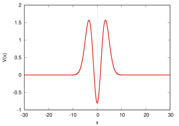
  Figure 1: Our model potential $V(x)=(\ref{V-Jolanta})$.

  One can see that $V(x)$ is a symmetric potential consisting of a single well and two barriers.
  A simple numerical algorithm of Appendix V can now be employed
  to calculate the corresponding energy dependent transmission probability $\Bigl{|}\,T_{E(+1)}^{+}\,\Bigr{|}^{2}$.
  The resulting outcome is depicted below:

  
  

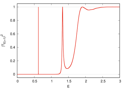
  Figure 2: The calculated transmission probability $\Bigl{|}\,T_{E(+1)}^{+}\,\Bigr{|}^{2}$.

  Note in passing that $T_{E(+1)}^{+}=T_{E(-1)}^{+}=T_{E}^{+}$ as stated by equation (231) of Appendix II.

  Lecture #4
  

  Fig.2 shows that the obtained profile of $\Bigl{|}\,T_{E(+1)}^{+}\,\Bigr{|}^{2}$ exhibits the following behavior:

  • For $E\to 0$ one encounters $\Bigl{|}\,T_{E(+1)}^{+}\,\Bigr{|}^{2}\to 0$. This agrees with physics intuition.
    $[\,$Low energy particles approaching our potential are always reflected back.$\,]$

  • For $E\to+\infty$ one encounters $\Bigl{|}\,T_{E(+1)}^{+}\,\Bigr{|}^{2}\to 1$. This agrees with physics intuition, too.
    $[\,$High energy particles approaching our potential are always transmitted.$\,]$

  • Most importantly, the profile of $\Bigl{|}\,T_{E(+1)}^{+}\,\Bigr{|}^{2}$ is not smooth, but contains sharp peaks.
    This phenomenon seems counter-intuitive and hardly explainable
    using the theory presented up to now in the present course.
    Indeed, one may wonder why there is an almost unit transmission for $E\doteq 0.621$,
    but almost zero transmission at $E=0.620$ or $E=0.622$.
    Similarly for the peak observed at $E\doteq 1.327$ and eventually for the higher peaks.

  The behavior of $\Bigl{|}\,T_{E(+1)}^{+}\,\Bigr{|}^{2}$ described in iii) is an example of a resonance phenomenon.
  An adequate theoretical explanation of the just touched resonance phenomena
  is outside the scope of the hermitian scattering theory.
  Desire of physics theoreticians to deeper understand the resonance phenomena
  has motivated an intense research activity, leading to the development of the so called
  nonhermitian scattering theory or nonhermitian quantum mechanics.
  This nonhermitian theory
  still remains an active field of research which continues to flourish even nowadays.
  One elegant version of the nonhermitian scattering theory
  is developed in the subsequent Part C of our course.

  Lecture #4
  

• B.14 Final summary of the conventional scattering theory in 1D
  Our introduction to the standard or orthodox scattering theory in 1D has been brought to an end.
  In Part A we have looked at scattering from the time dependent perspective.
  The AC was formulated, leading to entities $|\psi\rangle$, $|\phi_{\rm in}\rangle$, $|\phi_{\rm out}\rangle$ and ultimately to $\hat{S}$.
  We discussed physical meaning of the scattering matrix elements.
  Part B was motivated by our desire to switch from the time domain into the energy domain.
  In order to reach such a fundamental goal, we needed to proceed in multiple steps.
  Stated briefly, a more explicit interconnection between $|\psi\rangle$ and $|\phi_{\rm in}\rangle$ or $|\phi_{\rm out}\rangle$ has been established,
  through abstractly looking formulas (28) and (29). Subsequently, formulas (28) and (29)
  were replaced by equivalent yet time independent relations $[\,$(33), (36), (38), (40), (44), (50)$\,]$.
  The LSE (44) and (50) have led to the concept of stationary scattering states $|\psi_{E(\pm 1)}^{\pm}\rangle$,
  which were uniquely characterized by basic equations $[\,$(54), (55), (59), (61)-(70)$\,]$,
  and which were shown to possess the orthonormality property (80).
  Proceeding further on, by taking an advantage of the LSE (44) and (50),
  we were able to explicitly view the scattering operator $\hat{S}$ (and the closely related operator $\hat{T}$)
  solely in terms of the time independent entities $|\psi_{E(\pm 1)}^{\pm}\rangle$.
  See the most important relations $[\,$(85), (86), (87), (88), (89), (96), (97)$\,]$.
  We recall also formula (98) enabling us to calculate the scattering matrix elements (21),
  and the associated (experimentally measurable) transition probabilities (22).
  In the next step, we have illuminated the physical contents of $\hat{S}$ and $\hat{T}$
  by studying transmission/reflection of our quantum particle
  through/from the interaction region of the potential.
  Formulas (108)-(109) lead us towards the concept of the transmission/reflection coefficient,
  while in equations (113)-(114) we have determined
  the corresponding transmission/reflection probabilities.
  Finally, an illustrative numerical example was supplied,
  which has also highlighted an existence of scattering resonances.
  Thus, all in all, the general time independent scattering theory in 1D has been built up,
  and Part B can be closed. We hope that Part B has convinced the readers that
  the time independent approach to scattering is not only advantageous computationally,
  but leads also to deep physics insights.

Lecture #5

C. Nonhermitian Scattering Theory

Based upon Ref. [4].

• C.1 Motivational considerations
  In Part A we have introduced the basic theoretical setup of quantum scattering theory,
  via looking at scattering phenomena from the time dependent perspective.
  The AC was formulated, leading to entities $|\psi\rangle$, $|\phi_{\rm in}\rangle$, $|\phi_{\rm out}\rangle$ and ultimately to $\hat{S}$.
  Operator $\hat{S}$ was shown to contain all the information about an overall scattering outcome.
  We discussed physical meaning of the matrix elements of $\hat{S}$.
  In Part B we have developed the conventional or orthodox scattering theory,
  based upon switching from the time domain (wavepackets)
  into the energy domain (continuum eigenstates of the total Hamiltonian $\hat{\sf H}$).
  Central ingredient of this approach was the LSE (44) and (50).
  The just mentioned conventional or orthodox formulation is undoubtedly valid, exact, general,
  and used by vast majority of researchers working in scattering theory.
  But, remember, the whole energy domain formalism of Part B
  (time independent scattering theory, LSE)
  represents merely a tool for constructing $\hat{S}$ and for understanding its properties.
  In physics we are ultimately interested in the mapping $|\psi_{\rm out}\rangle\,=\,\hat{S}\,|\phi_{\rm in}\rangle$ of equation (18),
  not in the stationary eigenstates of $\hat{\sf H}$.
  By the way, the continuum eigenstates of $\hat{\sf H}$ are not square integrable,
  so they do not represent legitimate physical state vectors of quantum mechanics.
  Taking into account these remarks … one may reasonably ask now:
  Is there just a single possible way of studying the scattering phenomena ?
  $[\,$$\equiv$ the one outlined above in Part B ?$\,]$
  Or, are there other possible ways of getting $\hat{S}$
  and the associated physical information about scattering ?
  If yes, do these alternative ways possess any merits/offer any benefits
  compared to the above outlined conventional approach of Part B ?
  Stated concisely, an answer to these questions looks as follows.
  Nowadays there exist two alternative routes leading towards $\hat{S}$
  and to the associated scattering observables, namely:

  • Wavepacket propagation in the time domain
    Meaning that one solves the time dependent Schrödinger equation (4) numerically for a given incoming state $|\phi_{\rm in}\rangle$ and gets thus the corresponding outgoing state $|\phi_{\rm out}\rangle$. No need to deal with the energy domain, or continuum eigenstates of $\hat{\sf H}$, or LSE. Such a strategy looks somewhat like a ”brute force” approach based upon heavy computing, but some pragmatically oriented people prefer this style.

    Lecture #5
    

  • Nonhermitian scattering theory (and this we should study from now on)
    Motivated by our desire to better understand resonance phenomena and related matters.
    $[\,$Resonances $\sim$ rather unexpected and often sharp peaks in the transmission profile $\Bigl{|}\,T_{E(+1)}^{+}\,\Bigr{|}^{2}$.$\,]$
    Based upon solving an eigenvalue problem

    $$\left(\,-\,\frac{\hbar^{2}}{2\,m}\,\partial_{xx}\,+\,V(x)\,\right)\varphi_{j}(x)\;=\;E_{j}\,\varphi_{j}(x)\hskip 14.22636pt;$$ (117)

    where the eigenvalue $E_{j}$ is now allowed to be complex valued,
    and where the pertinent eigenfunction $\varphi_{j}(x)$ satisfies the so called Siegert boundary conditions
    $[\,$see our more detailed discussion below, especially Eqs. (124) and (126)$\,]$.
    Complex valued $E_{j}$’s indicate where the word ”nonhermitian” comes from.
    $[\,$Hermitian operators of the standard quantum mechanics have only real eigenvalues.$\,]$
    As we shall see later on, knowledge of $\{E_{j},\varphi_{j}(x)\}_{j}$ enables us to build $\hat{S}$
    and describe thus adequately all the scattering phenomena.
    Moreover, when the nonhermitian formulation of the problem is adopted,
    the concept of a resonance becomes sharply defined,
    and the role of resonances in scattering processes is then far better understood.
    In addition, the nonhermitian formalism itself is valuable by its own right,
    since it allows us to look at the scattering problems from an unconventional perspective.
    This in turn often leads towards a compelling physical interpretation
    and facilitates predictions of novel unexpected phenomena
    which are difficult to anticipate when working within the conventional formalism of Part B.

  The three above discussed approaches to scattering theory
  $[\,$0) conventional or orthodox, 1) wavepacket based, 2) nonhermitian ]
  are complementary, each of them possesses its own advantages and disadvantages.
  The real expert should ideally be conversant both with 0) and 1) and 2),
  and be able to combine these approaches neatly
  while taking into account specific features of a concrete quantum mechanical problem under study.

  Lecture #5
  

• C.2 Interlude: Bound states in the standard (hermitian) quantum mechanics
  Before elaborating more on the nonhermitian scattering theory, let us prepare the ground a bit,
  by recalling the solution of equation (117) for the case of bound states.
  $[\,$This is a standard stuff which can be found in any conventional textbook on quantum mechanics.$\,]$
  Let the range $(a,b)$ of our potential $V(x)$
  be conveniently changed into $(-a,+a)$ from now onwards $[\,$here $a>0$ is a prescribed parameter$\,]$.
  Suppose that $E_{j}$ and $\varphi_{j}(x)$ is a bound state solution of equation (117). Then $E_{j}<0$ as we know.
  In the right asymptotic region of $x>(+a)$, equation (117) reduces to

  $$-\,\frac{\hbar^{2}}{2\,m}\,\partial_{xx}\,\varphi_{j}(x)\;=\;E_{j}\,\varphi_{j}(x)\hskip 14.22636pt.$$ (118)

  General solution of (118) takes of course an explicit form

  $$\varphi_{j}(x)\;=\;{\cal A}_{+}\,e^{+\kappa_{j}x}\;+\;{\cal A}_{-}\,e^{-\kappa_{j}x}\hskip 14.22636pt;$$ (119)

  where

  $$\kappa_{j}\;=\;\sqrt{(-2)\,m\,E_{j}}/\hbar\hskip 14.22636pt;$$ (120)

  while ${\cal A}_{\pm}$ are as yet arbitrary complex coefficients. Note that $\kappa_{j}>0$.
  Since we are dealing with a bound state,
  the coefficient ${\cal A}_{+}$ pertaining to the exploding exponential $e^{+\kappa_{j}x}$ must vanish, thereby

  $$\varphi_{j}(x\to+\infty)\;\sim\;e^{-\kappa_{j}x}\hskip 14.22636pt.$$ (121)

  Similar sequence of arguments applies also for the left asymptotic region of $x\leq(-a)$.
  One encounters again (118), with the general solution $\varphi_{j}(x)={\cal B}_{+}\,e^{+\kappa_{j}x}+\,{\cal B}_{-}\,e^{-\kappa_{j}x}$ $({\rm here}\;\,{\cal B}_{\pm}\in{\mathbb{C}})$.
  Since we are dealing with a bound state,
  the coefficient ${\cal B}_{-}$ pertaining to the exploding exponential $e^{-\kappa_{j}x}$ must vanish, thereby

  $$\varphi_{j}(x\to-\infty)\;\sim\;e^{+\kappa_{j}x}\hskip 14.22636pt.$$ (122)

  Properties (121) and (122) indicate that $\varphi_{j}(x)$ behaves in the asymptotic region of $x\to\pm\infty$
  as a single exponential $e^{\mp\kappa_{j}x}$, not as a superposition of two exponentials.
  This observation will be recalled in the next paragraph,
  where it will motivate us to introduce the Siegert boundary conditions.
  Before proceeding further, let us make one additional remark regarding the bound state quantization.
  Namely, quantization of the bound state energy levels $E_{j}$ arises due to imposing
  two boundary conditions (121) and (122) on the solutions of the second order ODE (117). Indeed,
  while the ODE (117) possesses always two linearly independent particular solutions
  for any trial $E_{j}$ (even for $E_{j}$ complex),
  the two boundary conditions (121) and (122) can simultaneously be met
  only for a discrete set of specific eigenenergies.
  $[\,$See again any standard quantum mechanics textbook for details.
  $[\,$For bound states we require additionally $E_{j}$ to be real and negative.$\,]$
  

  Lecture #5
  

• C.3 Nonhermitian Quantum Mechanics: Introducing the Siegert states
  In the previous paragraph we have dealt with the bound state solutions of equation (117).
  Let us conveniently introduce the bound state problem once again using a slightly different language.
  Namely, when looking for the bound states of a given short ranged potential $V(x)$,
  we are interested in solutions $E_{j}$ and $\varphi_{j}(x)$ of an eigenvalue problem

  $${\color[rgb]{1,0,0}\left(\,-\,\frac{\hbar^{2}}{2\,m}\,\partial_{xx}\,+\,V(x)\,\right)\varphi_{j}(x)\;=\;E_{j}\,\varphi_{j}(x)\hskip 14.22636pt;}$$ (123)

  subjected to the boundary conditions

  $${\color[rgb]{1,0,0}\varphi_{j}(x\to+\infty)\;\sim\;e^{-ik_{j}x}\hskip 14.22636pt,\hskip 14.22636pt\varphi_{j}(x\to-\infty)\;\sim\;e^{+ik_{j}x}\hskip 14.22636pt;}$$ (124)

  where by definition

  $$k_{j}\;=\;\sqrt{2\,m\,E_{j}}/\hbar\hskip 14.22636pt.$$ (125)

  The associated energy eigenvalue $E_{j}$ is required to be real and negative for the case of bound states.
  Instead of (124) one may write equivalently

  $${\color[rgb]{1,0,0}\Bigl{(}\partial_{x}\,+\,i\,k_{j}\Bigr{)}\,\varphi_{j}(x)\Bigr{|}_{x=+a}=\;0\hskip 14.22636pt,\hskip 14.22636pt\Bigl{(}\partial_{x}\,-\,i\,k_{j}\Bigr{)}\,\varphi_{j}(x)\Bigr{|}_{x=-a}=\;0\hskip 14.22636pt.}$$ (126)

  Here, as we recall, symbol $a>0$ stands for the potential range $[\,$such that $V(x)=0$ for $|x|\geq a$$\,]$.
  It is a simple matter to verify that (124) implies (126) and vice versa.
  Most importantly, the nonhermitian quantum mechanics
  generalizes the notion of a bound state into the so called Siegert state.
  Namely, when looking for the Siegert states of a given short ranged potential $V(x)$,
  we are interested in solutions $E_{j}$ and $\varphi_{j}(x)$ of an eigenvalue problem (123)
  subjected to the Siegert boundary conditions (124) or (126). Definition (125) remains valid,
  yet the eigenvalue ${\bm{E}}_{\bm{j}}$ is allowed to be generally complex.
  Hence $k_{j}=(\ref{k-j-from-E-j})$ is also generally complex (not just negative imaginary as for the bound states),
  and the exponentials $e^{\mp ik_{j}x}$ appearing in (124) might be exploding!
  Bound states are apparently special cases of the Siegert states.
  If a given Siegert state solution $\varphi_{j}(x)$ of (123)-(124)/(126) explodes at $x\to\pm\infty$,
  then it is not square integrable and not normalizable in the usual sense.
  $[\,$The normalization issue is left unresolved for now, we will come to it later on in the course.$\,]$
  Not only the bound states,
  but all the Siegert state solutions $E_{j}$ and $\varphi_{j}(x)$ defined by equations (123)-(124)/(126)
  possess quantized (discrete) energy levels (some of these being complex).
  Indeed, quantization of $E_{j}$ arises in this context again due to imposing
  two boundary conditions (124)/(126) on the solutions of the second order ODE (123).
  While the ODE (123) possesses
  always two linearly independent particular solutions for any trial complex $E_{j}$,
  the two boundary conditions (124)/(126) can simultaneously be met
  only for a discrete set of specific eigenenergies.

  Lecture #5
  

• C.4 Looking at the Siegert states once again
  So far we have just defined the Siegert states $\varphi_{j}(x)$
  as solutions of the mathematical eigenvalue problem (123)-(124)/(126).
  Now it is appropriate to ask the following important questions:

  • How can one calculate all these Siegert states in practice (numerically)
    for a given potential $V(x)$ ?

  • How about normalization ? How about the orthonormality and closure relations ?

  • What are the Siegert states $\varphi_{j}(x)$ actually good for ?
    How are they related to the scattering theory, and in particular to quantities like $\hat{S}$ or $T_{E(+1)}^{+}$
    (where $E>0$ is of course real valued and continuous) ?

  • Can the language of Siegert states provide deeper insights into such phenomena
    like e.g. resonance scattering ?

  All the just posed questions are addressed very explicitly in the paragraphs below,
  which describe an elegant and clear cut formulation developed
  by Oleg Tolstikhin in 1990’s and onwards [4].
  Note that the concept of a Siegert state was introduced by Gamow and Siegert back in 1930’s.
  However, it was only Tolstikhin in 1990’s who succeeded
  to bridge the gap between the world of Siegert states and the standard quantum scattering theory.
  It was Tolstikhin who sharpened fundamentally the Siegert state formalism
  and brought it to practical use.

• C.5 Developing the Siegert state formalism: Take #1
  Let us recall equations (123), (126)
  and define the Siegert states as solutions of the following eigenvalue problem:

  $${\color[rgb]{1,0,0}\left(\,-\,\frac{\hbar^{2}}{2\,m}\,\partial_{xx}\,+\,V(x)\,\right)\,\varphi(x)\;=\;E\,\,\varphi(x)\hskip 14.22636pt;}$$ (127)

  $${\color[rgb]{1,0,0}\Bigl{(}\,\partial_{x}\,-\,ik\,\Bigr{)}\,\varphi(x)\,\Bigr{|}_{x=+a}\;=\;0\hskip 14.22636pt;}$$ (128)

  $${\color[rgb]{1,0,0}\Bigl{(}\,\partial_{x}\,+\,ik\,\Bigr{)}\,\varphi(x)\,\Bigr{|}_{x=-a}\;=\;0\hskip 14.22636pt.}$$ (129)

  Here $k$ stands for an as yet unknown generally complex parameter
  which gives rise to the complex energy $E=\frac{\hbar^{2}k^{2}}{2\,m}$.
  Let $\{{\it b}_{\nu}(x)\}_{\nu}$ be an arbitrary complete orthonormal basis set on an interval $x\in[-a,+a]$,
  such that

  $$\int_{-a}^{+a}b_{\nu}^{*}(x)\,b_{\nu^{\prime}}(x)\;{\rm d}x\;=\;\delta_{\nu\nu^{\prime}}\hskip 14.22636pt.$$ (130)

  Note that the basis functions ${\it b}_{\nu}(x)$ are not constrained to vanish at the edges $x=\pm a$.
  $[\,$Completeness actually requires at least some of the $b_{\nu}$’s to be nonvanishing at $x=\pm a$.$\,]$
  For example one may take

  $$b_{\nu}(x)\;=\;\sqrt{\frac{2\,\nu+1}{2\,a}}\;P_{\nu}\left(\frac{x}{a}\right)\hskip 14.22636pt,\hskip 14.22636pt\nu\,=\,0,1,2,3\ldots\hskip 14.22636pt;$$ (131)

  with $P_{\nu}(u)$ being the conventional Legendre polynomials.
  

  Lecture #5
  

  Alternatively one may employ the Fourier basis set

  $$b_{\nu}(x)\;=\;\frac{e^{+i\,\nu\,\pi\,\frac{x}{a}}}{\sqrt{2\,a}}\hskip 14.22636pt,\hskip 14.22636pt\nu\,\in\,\{\ldots,-2,-1,0,+1,+2,\ldots\}\hskip 14.22636pt.$$ (132)

  The as yet unknown Siegert state wavefunction can be for $x\in[-a,+a]$ expanded as

  $${\color[rgb]{1,0,0}\varphi(x)\;=\;\sum_{\nu}\,c_{\nu}\,{\it b}_{\nu}(x)\hskip 14.22636pt;}$$ (133)

  where the coefficients $c_{\nu}$ remain to be determined.
  $[\,$Boundary condition (128) implies that
  $[\,$$\varphi(x\geq(+a))\,=\,{\cal C}_{+}\,e^{+ikx}$, similarly $\varphi(x\leq(-a))\,=\,{\cal C}_{-}\,e^{-ikx}$ due to (129).
  $[\,$Factors ${\cal C}_{\pm}$ are fixed by demanding continuity of $\varphi(x)$ at $x=\pm a$.$\,]$
  In order to find the as yet unknown expansion coefficients $c_{\nu}$
  we multiply (127) by ${\it b}_{\nu}^{*}(x)$ and integrate over $x\in[-a,+a]$. One gets

  $$-\,\frac{\hbar^{2}}{2\,m}\,\int_{-a}^{+a}{\it b}_{\nu}^{*}(x)\,\partial_{xx}\,\varphi(x)\;{\rm d}x\;\,+\;\,\int_{-a}^{+a}{\it b}_{\nu}^{*}(x)\,\Bigl{(}V(x)-E\Bigr{)}\,\varphi(x)\;{\rm d}x\;=\;0\hskip 14.22636pt.$$ (134)

  Subsequently we integrate the first term by parts,
  and incorporate the Siegert boundary conditions (128)-(129).
  We also insert the basis set expansion (133) afterwards.
  This yields an intermediate outcome

  $$-\,\frac{i\hbar^{2}k}{2\,m}\,\sum_{\nu^{\prime}}\,c_{\nu^{\prime}}\,\Bigl{(}\,{\it b}_{\nu}^{*}(+a)\,{\it b}_{\nu^{\prime}}(+a)\,+\,{\it b}_{\nu}^{*}(-a)\,{\it b}_{\nu^{\prime}}(-a)\,\Bigr{)}\;+\;\frac{\hbar^{2}}{2\,m}\;\sum_{\nu^{\prime}}\,c_{\nu^{\prime}}\int_{-a}^{+a}\Bigl{(}\partial_{x}{\it b}_{\nu}^{*}(x)\Bigr{)}\Bigl{(}\partial_{x}{\it b}_{\nu^{\prime}}(x)\Bigr{)}\,{\rm d}x$$

  $$+\;\sum_{\nu^{\prime}}\,c_{\nu^{\prime}}\int_{-a}^{+a}{\it b}_{\nu}^{*}(x)\,V(x)\,{\it b}_{\nu^{\prime}}(x)\;{\rm d}x\;-\;\frac{\hbar^{2}k^{2}}{2\,m}\;c_{\nu}\;=\;0\hskip 14.22636pt.$$ (135)

  Next, let us conveniently translate formula (•) into the language of linear algebra.
  For this purpose we shall introduce the following matrix elements:

  $${\color[rgb]{1,0,0}H_{\nu\nu^{\prime}}} {\color[rgb]{1,0,0}=} {\color[rgb]{1,0,0}\frac{\hbar^{2}}{2\,m}\,\int_{-a}^{+a}\Bigl{(}\partial_{x}{\it b}_{\nu}^{*}(x)\Bigr{)}\Bigl{(}\partial_{x}{\it b}_{\nu^{\prime}}(x)\Bigr{)}\,{\rm d}x\;+\;\int_{-a}^{+a}{\it b}_{\nu}^{*}(x)\,V(x)\,{\it b}_{\nu^{\prime}}(x)\;{\rm d}x\hskip 14.22636pt;}$$ (136)

  $${\color[rgb]{1,0,0}L_{\nu\nu^{\prime}}} {\color[rgb]{1,0,0}=} {\color[rgb]{1,0,0}\frac{\hbar^{2}}{2\,m}\,\Bigl{(}\,{\it b}_{\nu}^{*}(+a)\,{\it b}_{\nu^{\prime}}(+a)\,+\,{\it b}_{\nu}^{*}(-a)\,{\it b}_{\nu^{\prime}}(-a)\,\Bigr{)}\hskip 14.22636pt.}$$ (137)

  Instead of (•) one may then write equivalently and concisely

  $${\color[rgb]{1,0,0}\left({\bm{H}}\,-\,i\,k\,{\bm{L}}\,-\,\frac{\hbar^{2}k^{2}}{2\,m}\,{\bm{I}}\right){\bm{c}}\;=\;{\bm{0}}\hskip 14.22636pt;}$$ (138)

  with obvious notations.

  Lecture #5
  

  Suppose that the basis set expansion (133) is truncated to $N$ terms
  (where $N$ is arbitrarily large in principle, it is of course restricted in practical calculations).
  The matrix equation (138) is then correspondingly truncated as well.
  $[\,$It contains then $N$-by-$N$ matrices ${\bm{H}}$, ${\bm{L}}$, ${\bm{I}}$ and and $N$-dimensional column vector ${\bm{c}}$.$\,]$
  Equation (138)$|_{N\,{\rm finite}}$ can now be classified as a quadratic eigenvalue problem of linear algebra,
  to be solved for unknowns $k$ and ${\bm{c}}$. An adequate solution of (138)$|_{N\,{\rm finite}}$ is performed
  by taking advantage of a linearization technique which is described in the next paragraph.
  For the sake of clarity, we point out here that equation (138)$|_{N\,{\rm finite}}$ or (138)$|_{N\to\infty}$ is implied
  by our original Siegert eigenvalue problem (127), (128)-(129). On the other hand,
  it is not obvious whether every solution $\{k,{\bm{c}}\}$ of equation (138)$|_{N\,{\rm finite}}$
  corresponds to some approximate Siegert eigenstate (133)
  which would satisfy (127), (128)-(129) in the limit of $N\to\infty$.
  For this reason we prefer to call all the solutions of (138)$|_{N\,{\rm finite}}$ as Siegert pseudostates.

  Lecture #6
  

• C.6 Developing the Siegert state formalism: Take #2
  The quadratic eigenvalue problem (138)$|_{N\,{\rm finite}}$ can be redisplayed in a more standard appearance

  $${\color[rgb]{1,0,0}\left({\bm{A}}\,+\,\lambda\,{\bm{B}}\,+\,\lambda^{2}\,{\bm{I}}\right){\bm{c}}\;=\;{\bm{0}}\hskip 14.22636pt;}$$ (139)

  where

  $${\color[rgb]{1,0,0}{\bm{A}}\;=\;+\,\frac{2\,m}{\hbar^{2}}\;{\bm{H}}\hskip 14.22636pt,\hskip 14.22636pt{\bm{B}}\;=\;-\,\frac{2\,m}{\hbar^{2}}\;{\bm{L}}\hskip 14.22636pt;}$$ (140)

  and

  $${\color[rgb]{1,0,0}\lambda\;=\;i\,k\hskip 14.22636pt.}$$ (141)

  To facilitate further progress and linearize the l.h.s. of (139) with respect to $\lambda$,
  we conveniently introduce a $2N$-component column vector

  $${\color[rgb]{1,0,0}\left(\matrix{{\bm{c}}\cr\bm{\tilde{}}{\bm{c}}}\right)\;=\;\left(\matrix{{\bm{c}}\cr\lambda\,{\bm{c}}}\right)\hskip 14.22636pt.}$$ (142)

  Equation (139) is then equivalent to

  $$\left(\matrix{{\bm{O}}&{\bm{I}}\cr-{\bm{A}}&-{\bm{B}}}\right)\left(\matrix{{\bm{c}}\cr\bm{\tilde{}}{\bm{c}}}\right)\;=\;\lambda\,\left(\matrix{{\bm{c}}\cr\bm{\tilde{}}{\bm{c}}}\right)\hskip 14.22636pt.$$ (143)

  Indeed, one may easily check that (139) implies (143) and vice versa.
  Importantly, the transformed problem (143) acquires doubled matrix dimension $2N$,
  yet it is linear in $\lambda$ as opposed to the $N$-dimensional matrix problem (139).
  $[\,$One may observe that the replacement (139) $\mapsto$ (143) resembles
  $[\,$the well known passage from a single second order ODE to two coupled first order ODEs.$\,]$
  Proceeding further, we multiply (143) by matrix

  $$\left(\matrix{{\bm{B}}&{\bm{I}}\cr{\bm{I}}&{\bm{O}}}\right)\hskip 14.22636pt;$$ (144)

  while noting that

  $$\left(\matrix{{\bm{B}}&{\bm{I}}\cr{\bm{I}}&{\bm{O}}}\right)^{-1}\;=\;\left(\matrix{{\bm{0}}&{\bm{I}}\cr{\bm{I}}&-{\bm{B}}}\right)\hskip 14.22636pt.$$ (145)

  $[\,$Due to (145) the matrix (144) is certainly regular.$\,]$ This converts equation (143) into an equivalent symmetric form

  $${\color[rgb]{1,0,0}\left(\matrix{-{\bm{A}}&{\bm{O}}\cr{\bm{O}}&{\bm{I}}}\right)\left(\matrix{{\bm{c}}\cr\bm{\tilde{}}{\bm{c}}}\right)\;=\;\lambda\,\left(\matrix{{\bm{B}}&{\bm{I}}\cr{\bm{I}}&{\bm{O}}}\right)\left(\matrix{{\bm{c}}\cr\bm{\tilde{}}{\bm{c}}}\right)\hskip 14.22636pt.}$$ (146)

  Symmetric linear eigenvalue problems (146) are treatable (even numerically)
  by standard well established methods of linear algebra.
  Hence also equations (139) and (138)$|_{N\,{\rm finite}}$ can be discussed and solved in this way.

  Lecture #6
  

• C.7 Developing the Siegert state formalism: Take #3
  Let us look again at problem (139), and define the corresponding quadratic matrix polynomial

  $${\color[rgb]{1,0,0}{\bm{M}}(\lambda)\;=\;{\bm{A}}\,+\,\lambda\,{\bm{B}}\,+\,\lambda^{2}\,{\bm{I}}\hskip 14.22636pt.}$$ (147)

  Instead of (139) one can write then

  $${\bm{M}}(\lambda)\;{\bm{c}}\;=\;{\bm{0}}\hskip 14.22636pt.$$ (148)

  The matrix equation (148) possesses a nontrivial solution ${\bm{c}}$ iff ${\rm det}[{\bm{M}}(\lambda)]=0$.
  But ${\rm det}[{\bm{M}}(\lambda)]$ is a $\lambda$-polynomial of degree $2N$.
  Polynomials of degree $2N$ generically have $2N$ distinct roots.
  Hereafter we shall assume, for the sake of maximum simplicity,
  that this is the case also for our polynomial equation ${\rm det}[{\bm{M}}(\lambda)]=0$.
  We shall also assume, again for the sake of maximum simplicity,
  that all the $2N$ roots of ${\rm det}[{\bm{M}}(\lambda)]=0$ are nonzero.
  $[\,$Correctness of the just made assumptions can always be checked by numerical calculation
  $[\,$performed a posteriori for each concrete physical system under study and for concrete $N$.$\,]$
  If so, equations (148), (146), (139) possess exactly $2N$ distinct eigensolutions

  $${\color[rgb]{1,0,0}\lambda^{(n)}\neq 0\hskip 14.22636pt,\hskip 14.22636pt\left(\matrix{{\bm{c}}^{(n)}\cr\bm{\tilde{}}{\bm{c}}^{(n)}}\right)\hskip 14.22636pt,\hskip 14.22636pt1\leq n\leq 2N\hskip 14.22636pt.}$$ (149)

  Here the eigenvectors are linearly independent due to (143) and (146).
  $[\,$Hence the $2N$ eigenvectors listed in (149) form a basis in the pertinent linear space ${\mathbb{C}}^{2N}$.$\,]$
  Correspondingly, in the finite basis set representation (138)$|_{N\,{\rm finite}}$
  of our original eigenvalue problem (127), (128)-(129)
  we have obtained exactly $2N$ distinct linearly independent Siegert pseudostates (133), that is,

  $${\color[rgb]{1,0,0}\varphi^{(n)}(x)\;=\;\sum_{\nu}\,c_{\nu}^{(n)}\,{\it b}_{\nu}(x)\hskip 14.22636pt.}$$ (150)

  The associated Siegert eigenvalue follows immediately from equation (141). One has

  $${\color[rgb]{1,0,0}k^{(n)}\;=\;-i\,\lambda^{(n)}\hskip 14.22636pt,\hskip 14.22636ptE^{(n)}\;=\;\frac{\hbar^{2}\left(k^{(n)}\right)^{2}}{2\,m}\;=\;-\,\frac{\hbar^{2}\left(\lambda^{(n)}\right)^{2}}{2\,m}\hskip 14.22636pt.}$$ (151)

  We have just finished answering question i) raised in the paragraph C.4.
  From now on we shall conveniently adopt the notation $\varphi^{(n)}(x)$
  instead of writing $\varphi_{j}(x)$ as we did tentatively in C.3-C.4.
  The same applies also for the pertinent eigenvalues $E^{(n)}$ and the related $k^{(n)}$.

  Lecture #6
  

• C.8 Developing the Siegert state formalism: Take #4
  Let us establish now appropriate orthonormality relations
  for the eigensolutions (149) of the problem (148), (146), (139).
  Take any two distinct eigensolutions (149), such that

  $$\left(\matrix{-{\bm{A}}&{\bm{O}}\cr{\bm{O}}&{\bm{I}}}\right)\left(\matrix{{\bm{c}}^{(n)}\cr\bm{\tilde{}}{\bm{c}}^{(n)}}\right)\;=\;\lambda^{(n)}\,\left(\matrix{{\bm{B}}&{\bm{I}}\cr{\bm{I}}&{\bm{O}}}\right)\left(\matrix{{\bm{c}}^{(n)}\cr\bm{\tilde{}}{\bm{c}}^{(n)}}\right)\hskip 14.22636pt;$$ (152)

  $$\left(\matrix{-{\bm{A}}&{\bm{O}}\cr{\bm{O}}&{\bm{I}}}\right)\left(\matrix{{\bm{c}}^{(n^{\prime})}\cr\bm{\tilde{}}{\bm{c}}^{(n^{\prime})}}\right)\;=\;\lambda^{(n^{\prime})}\,\left(\matrix{{\bm{B}}&{\bm{I}}\cr{\bm{I}}&{\bm{O}}}\right)\left(\matrix{{\bm{c}}^{(n^{\prime})}\cr\bm{\tilde{}}{\bm{c}}^{(n^{\prime})}}\right)\hskip 14.22636pt.$$ (153)

  Multiply (152) by $({\bm{c}}^{(n^{\prime})T},\bm{\tilde{}}{\bm{c}}^{(n^{\prime})T})$ and (153) by $({\bm{c}}^{(n)T},\bm{\tilde{}}{\bm{c}}^{(n)T})$. Subtract the two to get

  $$(\lambda^{(n)}-\lambda^{(n^{\prime})})\,\left(\matrix{{\bm{c}}^{(n)T}&\bm{\tilde{}}{\bm{c}}^{(n)T}}\right)\left(\matrix{{\bm{B}}&{\bm{I}}\cr{\bm{I}}&{\bm{O}}}\right)\left(\matrix{{\bm{c}}^{(n^{\prime})}\cr\bm{\tilde{}}{\bm{c}}^{(n^{\prime})}}\right)\;=\;0\hskip 14.22636pt.$$ (154)

  Formula (154) reveals that for $\lambda^{(n)}\neq\lambda^{(n^{\prime})}$ (and thus for $n\neq n^{\prime}$)
  the eigensolutions (149) are orthogonal with respect to the scalar product

  $$\left(\matrix{{\bm{c}}^{(n)T}&\bm{\tilde{}}{\bm{c}}^{(n)T}}\right)\left(\matrix{{\bm{B}}&{\bm{I}}\cr{\bm{I}}&{\bm{O}}}\right)\left(\matrix{{\bm{c}}^{(n^{\prime})}\cr\bm{\tilde{}}{\bm{c}}^{(n^{\prime})}}\right)\hskip 14.22636pt.$$ (155)

  Note also that for all values of $n$ $(1\leq n\leq 2N)$ we necessarily have

  $$\left(\matrix{{\bm{c}}^{(n)T}&\bm{\tilde{}}{\bm{c}}^{(n)T}}\right)\left(\matrix{{\bm{B}}&{\bm{I}}\cr{\bm{I}}&{\bm{O}}}\right)\left(\matrix{{\bm{c}}^{(n)}\cr\bm{\tilde{}}{\bm{c}}^{(n)}}\right)\;\neq\;0\hskip 14.22636pt.$$ (156)

  Since if the l.h.s. of (156) was zero for some $n$, then the vector $\left(\matrix{{\bm{B}}&{\bm{I}}\cr{\bm{I}}&{\bm{O}}}\right)\left(\matrix{{\bm{c}}^{(n)}\cr\bm{\tilde{}}{\bm{c}}^{(n)}}\right)$
  would be orthogonal to all the $2N$-dimensional vectors of our linear space ${\mathbb{C}}^{2N}$,
  hence $\left(\matrix{{\bm{B}}&{\bm{I}}\cr{\bm{I}}&{\bm{O}}}\right)\left(\matrix{{\bm{c}}^{(n)}\cr\bm{\tilde{}}{\bm{c}}^{(n)}}\right)$ would vanish, and thus also $\left(\matrix{{\bm{c}}^{(n)}\cr\bm{\tilde{}}{\bm{c}}^{(n)}}\right)$ would vanish $[\,$cf. property (145)$\,]$.
  Our above made observations lead us towards imposing the normalization convention

  $${\color[rgb]{1,0,0}\left(\matrix{{\bm{c}}^{(n)T}&\bm{\tilde{}}{\bm{c}}^{(n)T}}\right)\left(\matrix{{\bm{B}}&{\bm{I}}\cr{\bm{I}}&{\bm{O}}}\right)\left(\matrix{{\bm{c}}^{(n^{\prime})}\cr\bm{\tilde{}}{\bm{c}}^{(n^{\prime})}}\right)\;=\;2\,\lambda^{(n)}\;\delta_{nn^{\prime}}\hskip 14.22636pt.}$$ (157)

  The extra factor $2\,\lambda^{(n)}$ appearing on the r.h.s. of (157) has been inserted
  for the sake mathematical convenience. Recall in this context that $\lambda^{(n)}\neq 0$ for all $n$.
  An equivalent version of (157) is obtained by exploiting (142) and reads as

  $${\color[rgb]{1,0,0}\Bigl{(}\,\lambda^{(n)}+\lambda^{(n^{\prime})}\Bigr{)}\,{\bm{c}}^{(n)T}{\bm{c}}^{(n^{\prime})}\;+\;{\bm{c}}^{(n)T}{\bm{B}}\,{\bm{c}}^{(n^{\prime})}\;=\;2\,\lambda^{(n)}\;\delta_{nn^{\prime}}\hskip 14.22636pt.}$$ (158)

  Lecture #6
  

• C.9 Developing the Siegert state formalism: Take #5
  Let us establish now appropriate closure relations
  for the eigensolutions (149) of the problem (148), (146), (139). As mentioned already,
  the $2N$ eigenvectors listed in (149) form a basis in the pertinent linear space ${\mathbb{C}}^{2N}$.
  Meaning that every $2N$-dimensional column vector $\left(\matrix{{\bm{u}}\cr{\bm{v}}}\right)$ can be expressed in the form

  $$\left(\matrix{{\bm{u}}\cr{\bm{v}}}\right)\;=\;\sum_{n=1}^{2N}\;q_{n}\left(\matrix{{\bm{c}}^{(n)}\cr\bm{\tilde{}}{\bm{c}}^{(n)}}\right)\hskip 14.22636pt;$$ (159)

  with the coefficients

  $$q_{n}\;=\;\frac{1}{2\,\lambda^{(n)}}\,\left(\matrix{{\bm{c}}^{(n)T}&\bm{\tilde{}}{\bm{c}}^{(n)T}}\right)\left(\matrix{{\bm{B}}&{\bm{I}}\cr{\bm{I}}&{\bm{O}}}\right)\,\left(\matrix{{\bm{u}}\cr{\bm{v}}}\right)\hskip 14.22636pt;$$ (160)

  as being implied by (157). Consider an $2N$-by-$2N$ matrix

  $${\bm{Q}}\;=\;\sum_{n=1}^{2N}\,\frac{1}{2\,\lambda^{(n)}}\,\left(\matrix{{\bm{c}}^{(n)}\cr\bm{\tilde{}}{\bm{c}}^{(n)}}\right)\left(\matrix{{\bm{c}}^{(n)T}&\bm{\tilde{}}{\bm{c}}^{(n)T}}\right)\hskip 14.22636pt.$$ (161)

  Clearly,

  $${\bm{Q}}\,\left(\matrix{{\bm{B}}&{\bm{I}}\cr{\bm{I}}&{\bm{O}}}\right)\left(\matrix{{\bm{u}}\cr{\bm{v}}}\right)\;=\;\left(\matrix{{\bm{u}}\cr{\bm{v}}}\right)\hskip 14.22636pt;$$ (162)

  valid for all $\left(\matrix{{\bm{u}}\cr{\bm{v}}}\right)$. Meaning that

  $${\bm{Q}}\;=\;\left(\matrix{{\bm{B}}&{\bm{I}}\cr{\bm{I}}&{\bm{O}}}\right)^{-1}\;=\;\left(\matrix{{\bm{O}}&{\bm{I}}\cr{\bm{I}}&-{\bm{B}}}\right)\hskip 14.22636pt;$$ (163)

  cf. equation (145). From (161) and (163) one obtains using (142)
  the following important closure properties:

  $${\color[rgb]{1,0,0}\sum_{n=1}^{2N}\,\frac{1}{\lambda^{(n)}}\;{\bm{c}}^{(n)}\,{\bm{c}}^{(n)T}\;=\;{\bm{O}}\hskip 14.22636pt;}$$ (164)

  $${\color[rgb]{1,0,0}\sum_{n=1}^{2N}\,{\bm{c}}^{(n)}\,{\bm{c}}^{(n)T}\;=\;2\,{\bm{I}}\hskip 14.22636pt;}$$ (165)

  $${\color[rgb]{1,0,0}\sum_{n=1}^{2N}\,\lambda^{(n)}\;{\bm{c}}^{(n)}\,{\bm{c}}^{(n)T}\;=\;-2\,{\bm{B}}\hskip 14.22636pt.}$$ (166)

  We have just finished answering question ii) raised in the paragraph C.4.

  Lecture #6
  

• C.10 Developing the Siegert state formalism: Take #6
  As the last step of our formal mathematical elaborations
  we shall derive spectral representation of the inverse of the quadratic matrix polynomial (147).
  We claim that

  $${\color[rgb]{1,0,0}{\bm{M}}^{-1}(\lambda)\;=\;\sum_{n=1}^{2N}\,\frac{{\bm{c}}^{(n)}\,{\bm{c}}^{(n)T}}{2\,\lambda^{(n)}(\lambda-\lambda^{(n)})}\hskip 14.22636pt;}$$ (167)

  valid for all complex $\lambda$ except of course of the roots $\lambda^{(n)}$ of equation ${\rm det}[{\bm{M}}(\lambda)]=0$.
  In order to prove (167), we shall multiply both sides by ${\bm{M}}(\lambda)$ from the left,
  and see what comes out. One has

  $${\bm{M}}(\lambda)\;{\bm{M}}^{-1}(\lambda)\;=\;\sum_{n=1}^{2N}\,\frac{{\bm{M}}(\lambda)\,{\bm{c}}^{(n)}\,{\bm{c}}^{(n)T}}{2\,\lambda^{(n)}(\lambda-\lambda^{(n)})}\hskip 14.22636pt.$$ (168)

  But ${\bm{M}}(\lambda)\,{\bm{c}}^{(n)}\,=\,{\bm{M}}(\lambda_{n})\,{\bm{c}}^{(n)}\,+\,(\lambda-\lambda^{(n)})\,\Bigl{(}{\bm{B}}+(\lambda+\lambda^{(n)}){\bm{I}}\Bigr{)}\,{\bm{c}}^{(n)}$. Hence

  $${\bm{M}}(\lambda)\;{\bm{M}}^{-1}(\lambda)\;=\;\sum_{n=1}^{2N}\,\frac{\Bigl{(}{\bm{B}}+(\lambda+\lambda^{(n)}){\bm{I}}\Bigr{)}\,{\bm{c}}^{(n)}\,{\bm{c}}^{(n)T}}{2\,\lambda^{(n)}}\;=\;{\bm{I}}\hskip 14.22636pt;$$ (169)

  as a direct consequence of (164)-(165). The validity of (167) is thus established.

• C.11 Siegert state representation of the retarded Green function: Take #1
  Having passed through all the necessary mathematical preparations,
  we are slowly moving on towards addressing the question iii) raised in paragraph C.4.
  Most importantly, the gap between
  the mathematical world of Siegert states and the physical world of quantum scattering theory
  is bridged via examining the retarded (outgoing) Green function $G_{E}^{+}(x,y)$
  which has been introduced and discussed at length in Appendix IV.
  According to equations (274) and (294) from Appendix IV,
  an entity $G_{E}^{+}(x,y)$ is defined as an unique solution of the following boundary value problem:

  $${\color[rgb]{1,0,0}\left\{\,-\,\frac{\hbar^{2}}{2\,m}\,\partial_{xx}\,+\,V(x)\,-\,E\,\right\}\,G_{E}^{+}(x,y)\;=\;-\,\delta(x-y)\hskip 14.22636pt;}$$ (170)

  $$G_{E}^{+}(x\,_{<\,\min(-a,y)}^{>\,\max(+a,y)},y)\;\simeq\;e^{\pm ikx}\hskip 14.22636pt.$$ (171)

  Here $E>0$ stands for the physical impact energy and $k=\sqrt{2\,m\,E}/\hbar$ as usual.
  Let us hereafter assume $y\in[-a,+a]$. Requirement (171)
  can then be replaced by the Siegert type boundary conditions analogous to (128)-(129), that is,

  $${\color[rgb]{1,0,0}\Bigl{(}\,\partial_{x}\,-\,ik\,\Bigr{)}\,G_{E}^{+}(x,y)\,\Bigr{|}_{x=+a}\;=\;0\hskip 14.22636pt;}$$ (172)

  $${\color[rgb]{1,0,0}\Bigl{(}\,\partial_{x}\,+\,ik\,\Bigr{)}\,G_{E}^{+}(x,y)\,\Bigr{|}_{x=-a}\;=\;0\hskip 14.22636pt.}$$ (173)

  If so, then our boundary value problem (170), (172)-(173) may be for $|y|\leq a$ analyzed and solved
  using the same method as we applied above for the Siegert eigenproblem (127), (128)-(129).

  Lecture #6
  

  Namely, let us restrict $x$ like we did for $y$, such that $x,y\in[-a,+a]$,
  and expand $G_{E}^{+}(x,y)$ similarly as done in (133) for the case of $\varphi(x)$. This amounts to set

  $$G_{E}^{+}(x,y)\;=\;\sum_{\nu\nu^{\prime}}\,G_{E,\nu\nu^{\prime}}^{+}\,{\it b}_{\nu}(x)\,{\it b}_{\nu^{\prime}}(y)\hskip 14.22636pt;$$ (174)

  where the as yet unknown expansion coefficients $G_{E,\nu\nu^{\prime}}^{+}$ remain to be determined.
  Much as before in (133),
  the summation over $\nu$ is truncated in (174) just to $N$ terms, and similarly for $\nu^{\prime}$.
  In order to find the $N^{2}$ matrix elements $G_{E,\nu\nu^{\prime}}^{+}$, we multiply (170) by ${\it b}_{\nu}^{*}(x)\,{\it b}_{\nu^{\prime}}^{*}(y)$,
  and integrate over both spatial coordinates $x,y\in[-a,+a]$.
  This yields, with the help of (130), a preliminary formula

  $$-\,\frac{\hbar^{2}}{2\,m}\,\int_{-a}^{+a}{\rm d}x\int_{-a}^{+a}{\rm d}y\;\,{\it b}_{\nu}^{*}(x)\,{\it b}_{\nu^{\prime}}^{*}(y)\;\partial_{xx}\,G_{E}^{+}(x,y)$$

  $$+\;\int_{-a}^{+a}{\rm d}x\int_{-a}^{+a}{\rm d}y\;\,{\it b}_{\nu}^{*}(x)\,{\it b}_{\nu^{\prime}}^{*}(y)\,\Bigl{(}V(x)-E\Bigr{)}\,G_{E}^{+}(x,y)\;=\;-\,\delta_{\nu\nu^{\prime}}\hskip 14.22636pt.$$

  Subsequently we integrate the first term of (•) by parts,
  and incorporate the Siegert boundary conditions (172)-(173).
  We also insert the basis set expansion (174) afterwards,
  and take again an advantage of (130).
  All the mentioned manipulations provide altogether an intermediate outcome

  $$-\,\frac{i\hbar^{2}k}{2\,m}\,\sum_{\nu^{\prime\prime}}\,G_{E,\nu^{\prime\prime}\nu^{\prime}}^{+}\,\Bigl{(}\,{\it b}_{\nu}^{*}(+a)\,{\it b}_{\nu^{\prime\prime}}(+a)\,+\,{\it b}_{\nu}^{*}(-a)\,{\it b}_{\nu^{\prime\prime}}(-a)\,\Bigr{)}\;+\;\frac{\hbar^{2}}{2\,m}\;\sum_{\nu^{\prime\prime}}\,G_{E,\nu^{\prime\prime}\nu^{\prime}}^{+}\int_{-a}^{+a}\Bigl{(}\partial_{x}{\it b}_{\nu}^{*}(x)\Bigr{)}\Bigl{(}\partial_{x}{\it b}_{\nu^{\prime\prime}}(x)\Bigr{)}\,{\rm d}x$$

  $$+\;\sum_{\nu^{\prime\prime}}\,G_{E,\nu^{\prime\prime}\nu^{\prime}}^{+}\int_{-a}^{+a}{\it b}_{\nu}^{*}(x)\,V(x)\,{\it b}_{\nu^{\prime\prime}}(x)\;{\rm d}x\;-\;\frac{\hbar^{2}k^{2}}{2\,m}\;G_{E,\nu\nu^{\prime}}^{+}\;=\;-\,\delta_{\nu\nu^{\prime}}\hskip 14.22636pt;$$ (176)

  which means however nothing else than

  $${\color[rgb]{1,0,0}{\bm{G}}_{E}^{+}\,\left({\bm{H}}\,-\,i\,k\,{\bm{L}}\,-\,\frac{\hbar^{2}k^{2}}{2\,m}\,{\bm{I}}\right)\;=\;-\;{\bm{I}}\hskip 14.22636pt.}$$ (177)

  Here ${\bm{G}}_{E}^{+}$ stands of course for an $N$-by-$N$ matrix of elements $G_{E,\nu\nu^{\prime}}^{+}$.
  Matrices ${\bm{H}}$ and ${\bm{L}}$ are defined above in (136)-(137).
  Instead of (177) one may write equivalently

  $${\color[rgb]{1,0,0}{\bm{G}}_{E}^{+}\,\left({\bm{A}}\,+\,\lambda\,{\bm{B}}\,+\,\lambda^{2}\,{\bm{I}}\right)\;=\;-\,\frac{2\,m}{\hbar^{2}}\,{\bm{I}}\hskip 14.22636pt;}$$ (178)

  with the matrices ${\bm{A}}$ and ${\bm{B}}$ being given by prescription (140), and $\lambda=ik$ as in (141).
  Even more concisely we can state that

  $${\color[rgb]{1,0,0}{\bm{G}}_{E}^{+}\;{\bm{M}}(\lambda)\;=\;-\,\frac{2\,m}{\hbar^{2}}\,{\bm{I}}\hskip 14.22636pt;}$$ (179)

  where the matrix polynomial ${\bm{M}}(\lambda)=(\ref{bm-M-lambda-def})$.

  Lecture #6
  

• C.12 Siegert state representation of the retarded Green function: Take #2
  Our introduction to nonhermitian scattering theory approaches an epic final.
  In this paragraph and in the next one,
  all the above pursued technical developments of Part C come to fruition.
  Most importantly, equation (179) enables us to conclude that

  $${\bm{G}}_{E}^{+}\;=\;-\,\frac{2\,m}{\hbar^{2}}\;{\bm{M}}^{-1}(\lambda)\hskip 14.22636pt.$$ (180)

  Our previously obtained formula (167) implies in turn

  $${\color[rgb]{1,0,0}{\bm{G}}_{E}^{+}\;=\;\frac{m}{\hbar^{2}}\;\sum_{n=1}^{2N}\,\frac{{\bm{c}}^{(n)}\,{\bm{c}}^{(n)T}}{\lambda^{(n)}(\lambda^{(n)}-\lambda)}\hskip 14.22636pt;}$$ (181)

  or, in other words,

  $$G_{E,\nu\nu^{\prime}}^{+}\;=\;\frac{m}{\hbar^{2}}\;\sum_{n=1}^{2N}\,\frac{c_{\nu}^{(n)}\,c_{\nu^{\prime}}^{(n)}}{\lambda^{(n)}(\lambda^{(n)}-\lambda)}\hskip 14.22636pt.$$ (182)

  Subsequently one may combine (182) with (174) and (150).
  This yields a simple, fully explicit, and compelling result

  $${\color[rgb]{1,0,0}G_{E}^{+}(x,y)\;=\;\frac{m}{\hbar^{2}}\;\sum_{n=1}^{2N}\,\frac{\varphi^{(n)}(x)\;\varphi^{(n)}(y)}{\lambda^{(n)}(\lambda^{(n)}-\lambda)}\;=\;\frac{m}{\hbar^{2}}\;\sum_{n=1}^{2N}\,\frac{\varphi^{(n)}(x)\;\varphi^{(n)}(y)}{k^{(n)}(k-k^{(n)})}\hskip 14.22636pt.\hskip 14.22636pt[\,-a\leq x,y\leq+a\,]}$$ (183)

  Consistency of the whole mathematical formulation leading to (183)
  excludes an existence of singularities in the denominator term $(k-k^{(n)})^{-1}$.
  $[\,$Another remark: Boundary condition (172) implies that
  $[\,$$G_{E}^{+}(x\geq(+a),y)={\cal G}_{+}\,e^{+ikx}$, similarly $G_{E}^{+}(x\leq(-a),y)={\cal G}_{-}\,e^{-ikx}$ due to (173). $(\#)$
  $[\,$This holds of course assuming $|y|\leq a$.
  $[\,$Factors ${\cal G}_{\pm}$ are fixed by demanding continuity of $G_{E}^{+}(x,y)$ at $x=\pm a$.$\,]$
  Equation (183) and our comment $(\#)$ express
  the retarded Green function $G_{E}^{+}(x,y)$ of the conventional quantum scattering theory
  solely in terms of the nonhermitian Siegert pseudostates (150) and their pertinent eigenvalues (151).
  $[\,$We tacitly assume $(-a)\leq y\leq(+a)$ and $x\in(-\infty,+\infty)$ in the just presented statements.$\,]$
  We recall from Part B that knowledge of $G_{E}^{+}(x,y)$ for $|y|\leq a$
  enables us to straightforwardly determine
  the $\hat{T}$-operator and thus also the fundamental scattering operator $\hat{S}$
  $[\,$see equations (85), (88), (89)$\,]$. If so, then
  the entire quantum scattering theory can be reformulated
  solely in terms of the Siegert pseudostates $\left\{\lambda^{(n)},\,\varphi^{(n)}(x)\right\}_{n=1}^{2N}$
  which contain complete physical information about all the scattering phenomena.
  Valid of course as a well defined approximation,
  which becomes exact in the complete basis set limit of $N\to\infty$.
  As one can see, the fundamental equation (183) of Tolstikhin contains merely
  a discrete sum over all the $2N$ calculated Siegert pseudostates.
  The stationary scattering states $\psi_{E(\pm 1)}^{+}(x)$ of Part B are not referenced at all in (183).

  Lecture #6
  

• C.13 Siegert state representation of the transmission coefficient
  Let us supply now
  a concrete example of an application of the nonhermitian Siegert pseudostate formalism,
  namely, a Siegert based calculation of the transmission coefficient $T_{E}^{+}=T_{E(\pm 1)}^{+}$.
  $[\,$For the sake of clarity we recall in this context equation (231) of Appendix II.$\,]$
  We shall take advantage of the formula (308) which was derived in Appendix IV.
  When translated into our notation of Part C, equation (308) looks as follows:

  $$G_{E}^{+}(-a,+a)\;=\;\frac{(-i)\,m}{\hbar^{2}k}\;\,T_{E}^{+}\;\,e^{+2ika}\hskip 14.22636pt.$$ (184)

  Combination of (184) and (183) provides immediately
  an interesting, important, and explicit result

  $${\color[rgb]{1,0,0}T_{E}^{+}\;=\;i\;k\;e^{-2ika}\,\sum_{n=1}^{2N}\,\frac{\varphi^{(n)}(-a)\;\varphi^{(n)}(+a)}{k^{(n)}(k-k^{(n)})}\hskip 14.22636pt.}$$ (185)

  This demonstrates that the transmission coefficient $T_{E}^{+}$ of the conventional scattering theory
  is expressible solely in terms of the Siegert pseudostates.
  Formula (185) lends itself well to a numerical test.
  $[\,$As a benchmark one may take here our conventional calculation of $T_{E}^{+}=T_{E(\pm 1)}^{+}$
  $[\,$which was performed above in the paragraph B.13.
  $[\,$The just sketched program will be implemented in a very explicit fashion during our Project.$\,]$
  It is worthy to look again at equation (185) and examine its physical contents.
  In (185), the transmission coefficient $T_{E}^{+}$ is determined
  as a discrete sum over separate contributions of all the corresponding $2N$ Siegert pseudostates.
  For a particular physical system under study, and for a prescribed impact energy $E=\frac{\hbar^{2}k^{2}}{2m}$,
  it may sometimes happen that the physical value of $k$
  almost coincides with $k^{(n)}$ at some single $n$ (say at $n=1$).
  If so, then the $n=1$ term often dominates in the summation (185),
  and hence $T_{E}^{+}$ can be approximated just by

  $$T_{E}^{+}\;\doteq\;i\;k\;e^{-2ika}\;\frac{\varphi^{(1)}(-a)\;\varphi^{(1)}(+a)}{k^{(1)}(k-k^{(1)})}\hskip 14.22636pt.$$ (186)

  Suppose that $\varphi^{(1)}(x)$ solves the Siegert boundary value problem (127), (128)-(129).
  Then it is not hard to see that, necessarily, $\Re\,k^{(1)}>0$ and $\Im\,k^{(1)}<0$.
  $[\,$Indeed, since $k>0$ is close to $k^{(1)}$, then $\Re\,k^{(1)}>0$ and $\Im\,k^{(1)}$ is small in magnitude.
  $[\,$Furthermore, as we know, $\varphi^{(1)}(x\,^{>}_{<}\pm a)={\cal C}_{\pm}\,e^{\pm ik^{(1)}x}$.
  $[\,$For $\Im\,k^{(1)}>0$ the exponential $e^{\pm ik^{(1)}x}$ would decay with $x\to\pm\infty$,
  $[\,$thus $\varphi^{(1)}(x)$ would be a bound state pertinent to real $E^{(1)}$ and thus to real $k^{(1)}$, contradiction.
  $[\,$For $\Im\,k^{(1)}=0$, $\varphi^{(1)}(x)$ would be an ordinary continuum eigenstate of $\hat{\sf H}$ having real $E^{(1)}>0$,
  $[\,$yet this is inconsistent with the Siegert boundary conditions (128)-(129)
  $[\,$due to properties (115), (208).$\,]$
  Correspondingly, the associated complex energy eigenvalue $E^{(1)}=\,\hbar^{2}(k^{(1)})^{2}/(2\,m)$
  takes the form $E^{(1)}={\cal E}_{\rm res}^{(1)}-i\,\Gamma_{\rm res}^{(1)}/2$ where both ${\cal E}_{\rm res}^{(1)}>0$ and $\Gamma_{\rm res}^{(1)}>0$.
  We call $\varphi^{(1)}(x)$ as a resonance state.

  Lecture #6
  

  Equation (186) can be now further transformed, into

  $$T_{E}^{+}\;\doteq\;i\;\frac{\hbar^{2}}{2\,m}\left(\frac{k(k+k^{(1)})}{k^{(1)}}\right)e^{-2ika}\;\frac{\varphi^{(1)}(-a)\;\varphi^{(1)}(+a)}{E-E^{(1)}}\;\doteq\;i\;\frac{\hbar^{2}k^{(1)}}{m}\;e^{-2ika}\;\frac{\varphi^{(1)}(-a)\;\varphi^{(1)}(+a)}{E-{\cal E}_{\rm res}^{(1)}+i\,\Gamma_{\rm res}^{(1)}/2}\hskip 14.22636pt.$$ (187)

  The just obtained approximation (187) of the transmission coefficient $T_{E}^{+}=(\ref{Siegert-T-E-+-final})$
  is expected to work very accurately in an energy range of $E\approx{\cal E}_{\rm res}^{(1)}$,
  provided that $\Gamma_{\rm res}^{(1)}$ is small in magnitude compared to ${\cal E}_{\rm res}^{(1)}$, and provided that
  there are no other resonances $E^{(n)}={\cal E}_{\rm res}^{(n)}-i\,\Gamma_{\rm res}^{(n)}/2$ located nearby $E^{(1)}={\cal E}_{\rm res}^{(1)}-i\,\Gamma_{\rm res}^{(1)}/2$.
  Assuming that (187) holds reasonably well,
  the resulting transmission probability possesses for $E\approx{\cal E}_{\rm res}^{(1)}$ a Lorentzian form

  $${\color[rgb]{1,0,0}\Bigl{|}\,T_{E}^{+}\,\Bigr{|}^{2}\;\doteq\;{\cal Q}\;\frac{\left(\frac{\Gamma_{\rm res}^{(1)}}{2}\right)^{2}}{\left(E-{\cal E}_{\rm res}^{(1)}\right)^{2}+\left(\frac{\Gamma_{\rm res}^{(1)}}{2}\right)^{2}}\hskip 14.22636pt;}$$ (188)

  with a prefactor

  $${\cal Q}\;=\;\left|\,\frac{\hbar^{2}k^{(1)}}{m}\,\frac{2}{\Gamma_{\rm res}^{(1)}}\,\varphi^{(1)}(-a)\;\varphi^{(1)}(+a)\,\right|^{2}\hskip 14.22636pt.$$ (189)

  Formula (188) represents the so called
  Breit-Wigner profile of a resonance peak in the transmission probability.
  Let us revisit now our illustrative scattering calculation discussed in the paragraph B.13.
  We claim that each of the two sharp peaks of $\Bigl{|}\,T_{E}^{+}\,\Bigr{|}^{2}$ encountered in Fig.2 of B.13
  appears merely due to the resonance transmission phenomenon,
  which is described adequately by the nonhermitian equation (188).
  $[\,$Here apparently ${\cal Q}\doteq 1$, an explanation exists but reaches beyond the scope of our present course.$\,]$
  In other words, we anticipate that the two mentioned narrow transmission peaks of Fig.2
  arise due to presence of isolated resonances in our model potential $V(x)$
  $[\,$defined by equation (116) and plotted in Fig.1$\,]$.
  The just presented claim will be verified by an explicit numerical calculation
  during our computational Project.
  In the paragraphs C.12-C.13 we have answered, arguably quite convincingly,
  the fundamental questions iii) and iv) raised before in C.4.
  Our short introduction to nonhermitian scattering theory can thus be brought to an end.

Project

D. Mini-project: Transmission phenomena studied using the conventional scattering theory
and using the nonhermitian Siegert based approach

• The aim of this tutorial mini-project will be to investigate numerically
  the problem of scattering of a quantum particle in 1D.
  We shall focus on evaluating the transmission probability $\Bigl{|}\,T_{E}^{+}\,\Bigr{|}^{2}$
  as a function of the incident particle energy $E$, using two approaches:

  • The standard hermitian time independent scattering theory of Part B.
    See especially the paragraph B.13, which contains also the definition of our model problem.

  • The nonhermitian scattering theory, based upon the Siegert pseudostate formalism
    as outlined in Part C. See especially the paragraph C.13.

• Our first major goal will be to demonstrate that both theoretical frameworks a) and b)
  provide the same transmission profiles. $[\,$Which should be the same as plotted in Fig.2.$\,]$
  Our second goal will be to highlight fundamental advantage of the nonhermitian formalism
  $[\,$approach b)$\,]$ for the description of resonance scattering.
  This would amount to calculate explicitly the corresponding resonance wavefunctions $\varphi^{(n)}(x)$,
  and to identify their role in forming Lorentzian peaks (188) in the obtained transmission profile.

• Our third (optional) goal might be to proceed further
  by considering other suitable 1D potentials, and to try to understand the role
  of the so called exceptional points and/or anti-bound states in scattering phenomena.

Appendix I

Appendix I: Continuity equation and related matters

Based upon Refs. [1, 2].

• Consider the time dependent Schrödinger equation (4) in the position representation,

  $$i\hbar\;\partial_{t}\,\psi(t,x)\;=\;-\,\frac{\hbar^{2}}{2\,m}\,\partial_{xx}\,\psi(t,x)\;+\;V(x)\,\psi(t,x)\hskip 14.22636pt.$$ (190)

  Let $\psi(t,x)$ be any particular solution of (190),
  it can be a wavepacket but also a spatially delocalized function,
  depending upon the prescribed initial condition $\psi(t_{\rm init},x)$.
  A combination of formulas

  $$(+i)\hbar\;\partial_{t}\,\psi^{\phantom{*}}(t,x) = -\,\frac{\hbar^{2}}{2\,m}\,\partial_{xx}\,\psi^{\phantom{*}}(t,x)\;+\;V(x)\,\psi^{\phantom{*}}(t,x)$$ (191)

  $$(-i)\hbar\;\partial_{t}\,\psi^{*}(t,x) = -\,\frac{\hbar^{2}}{2\,m}\,\partial_{xx}\,\psi^{*}(t,x)\;+\;V(x)\,\psi^{*}(t,x)$$ (192)

  provides the following outcome,

  $$\partial_{t}\Bigl{(}\psi^{*}(t,x)\,\psi(t,x)\Bigr{)} = \frac{i\,\hbar}{2\,m}\,\Bigl{(}\,\psi^{*}(t,x)\,\partial_{xx}\,\psi(t,x)\,-\,\psi(t,x)\,\partial_{xx}\,\psi^{*}(t,x)\,\Bigr{)}\;=$$ (193)

  $$= \frac{i\,\hbar}{2\,m}\,\partial_{x}\Bigl{(}\,\psi^{*}(t,x)\,\partial_{x}\,\psi(t,x)\,-\,\psi(t,x)\,\partial_{x}\,\psi^{*}(t,x)\,\Bigr{)}\hskip 14.22636pt.$$

  Subsequently one gets

  $$\partial_{t}\Bigl{(}\psi^{*}(t,x)\,\psi(t,x)\Bigr{)}\;=\;-\,\partial_{x}\,\frac{1}{2}\left\{\,\psi^{*}(t,x)\left(\frac{\hat{\sf p}}{m}\,\psi(t,x)\right)\,-\,\psi(t,x)\left(\frac{\hat{\sf p}}{m}\,\psi(t,x)\right)^{*}\,\right\}\hskip 14.22636pt.$$ (194)

  After setting

  $$\varrho(t,x)\;=\;\psi^{*}(t,x)\,\psi(t,x)\hskip 7.11317pt,\hskip 7.11317ptJ(t,x)\;=\;\frac{1}{2}\left\{\,\psi^{*}(t,x)\left(\frac{\hat{\sf p}}{m}\,\psi(t,x)\right)\,-\,\psi(t,x)\left(\frac{\hat{\sf p}}{m}\,\psi(t,x)\right)^{*}\,\right\}$$ (195)

  one converts (194) into the desired continuity equation, namely,

  $$\partial_{t}\,\varrho(t,x)\;+\;\partial_{x}\,J(t,x)\;=\;0\hskip 14.22636pt.$$ (196)

  Recall that the continuity equation (196)
  expresses mathematically the law of probability conservation.
  It is valid for an arbitrary solution $\psi(t,x)$ of the time dependent Schrödinger equation (190).
  In particular, $\psi(t,x)$ does not need to be square integrable or spatially localized.

  Appendix I
  

• Equation (193) admits an additional and rather important generalization.
  Namely, let $\psi_{1}(t,x)$ and $\psi_{2}(t,x)$ be two arbitrary (generally distinct) particular solutions of (190).
  A combination of formulas

  $$(+i)\hbar\;\partial_{t}\,\psi_{2}^{\phantom{*}}(t,x) = -\,\frac{\hbar^{2}}{2\,m}\,\partial_{xx}\,\psi_{2}^{\phantom{*}}(t,x)\;+\;V(x)\,\psi_{2}^{\phantom{*}}(t,x)$$ (197)

  $$(-i)\hbar\;\partial_{t}\,\psi_{1}^{*}(t,x) = -\,\frac{\hbar^{2}}{2\,m}\,\partial_{xx}\,\psi_{1}^{*}(t,x)\;+\;V(x)\,\psi_{1}^{*}(t,x)$$ (198)

  provides the following outcome,

  $$\partial_{t}\Bigl{(}\psi_{1}^{*}(t,x)\,\psi_{2}(t,x)\Bigr{)} = \frac{i\,\hbar}{2\,m}\,\Bigl{(}\,\psi_{1}^{*}(t,x)\,\partial_{xx}\,\psi_{2}(t,x)\,-\,\psi_{2}(t,x)\,\partial_{xx}\,\psi_{1}^{*}(t,x)\,\Bigr{)}\;=$$ (199)

  $$= \frac{i\,\hbar}{2\,m}\,\partial_{x}\Bigl{(}\,\psi_{1}^{*}(t,x)\,\partial_{x}\,\psi_{2}(t,x)\,-\,\psi_{2}(t,x)\,\partial_{x}\,\psi_{1}^{*}(t,x)\,\Bigr{)}\hskip 14.22636pt.$$

  Valid again even if the solutions $\psi_{1,2}(t,x)$ of (190) are not square integrable or spatially localized.

• Let us revisit equation (199), and assume that both $\psi_{1}(t,x)$ and $\psi_{2}(t,x)$ are stationary states of $\hat{\sf H}$.
  Thus $\psi_{1,2}(t,x)\,=\,\psi_{E}^{(1,2)}(x)\;e^{-(i/\hbar)Et}$ with obvious notations.
  Equation (193) is correspondingly simplified into

  $$\partial_{x}\Bigl{(}\,\psi_{E}^{(1)*}(x)\,\partial_{x}\,\psi_{E}^{(2)}(x)\,-\,\psi_{E}^{(2)}(x)\,\partial_{x}\,\psi_{E}^{(1)*}(x)\,\Bigr{)}\;=\;0\hskip 14.22636pt.$$ (200)

  Subsequent integration over $x\in(a,b)$ yields then

  $$\Bigl{(}\,\psi_{E}^{(1)*}(x)\,\partial_{x}\,\psi_{E}^{(2)}(x)\,-\,\psi_{E}^{(2)}(x)\,\partial_{x}\,\psi_{E}^{(1)*}(x)\,\Bigr{)}\Bigr{|}_{x=a}^{x=b}\;=\;0\hskip 14.22636pt.$$ (201)

  Formula (201) will be exploited in Appendix II.

Appendix II

Appendix II: One-dimensional stationary Schrödinger equation

Based upon Refs. [1, 2].

• Let us consider an eigenvalue problem of the full Hamiltonian $\hat{\sf H}=(\ref{hat-sf-H-H0-V})$ in the position representation.
  One has

  $$\left\{\,-\,\frac{\hbar^{2}}{2\,m}\,\partial_{xx}\,+\,V(x)\,\right\}\psi_{E}(x)\;=\;E\,\psi_{E}(x)\hskip 14.22636pt.$$ (202)

  Here $\psi_{E}(x)$ is a provisional notation for the eigenfunctions.
  In what follows, we shall be concerned only with the continuum eigenstates of $\hat{\sf H}$,
  associated with $E>0$. We omit any discussion of eventual bound states.

• At any given $E>0$,
  the problem (202) represents a second order ordinary differential equation (ODE) for $\psi_{E}(x)$.
  Since our potential $V(x)$ vanishes for all $x\geq b$,
  it is legitimate to set $\psi_{E}(x\geq b)=e^{+iKx}$ with $\hbar K=\sqrt{2\,m\,E}$.
  Subsequent back propagation of the ODE (202) yields uniquely $\psi_{E}(x)$ also for all $x<b$.
  Since $V(x)$ vanishes for all $x\leq a$, the wavefunction $\psi_{E}(x\leq a)$
  is necessarily some linear combination of two exponentials $e^{\pm iKx}$.
  Thus $\psi_{E}(x\leq a)=A(E)\,e^{+iKx}+B(E)\,e^{-iKx}$,
  where $A(E)$ and $B(E)$ are some uniquely determined coefficients.
  Let us recall now formula (201) from Appendix I and set $\psi_{E}^{(1)}(x)=\psi_{E}^{(2)}(x)=\psi_{E}(x)$, such that

  $$\Bigl{(}\,\psi_{E}^{*}(x)\,\partial_{x}\,\psi_{E}(x)\,-\,\psi_{E}(x)\,\partial_{x}\,\psi_{E}^{*}(x)\,\Bigr{)}\Bigr{|}_{x=a}^{x=b}\;=\;0\hskip 14.22636pt.$$ (203)

  After plugging into (203) the above discussed simple explicit forms of $\psi_{E}(x\leq a)$ and $\psi_{E}(x\geq b)$,
  one finds that $|A(E)|^{2}=|B(E)|^{2}+1$. Showing that $A(E)$ is certainly nonzero.
  If so, one may redefine $\psi_{E}(x)$ via dividing it by $A(E)$.
  Then $\psi_{E}(x\leq a)=e^{+iKx}+R(E)\,e^{-iKx}$ and $\psi_{E}(x\geq b)=T(E)\,e^{+iKx}$,
  where $R(E)=B(E)/A(E)$ and $T(E)=1/A(E)$ are uniquely determined coefficients.
  Since $|A(E)|^{2}=|B(E)|^{2}+1$, one inevitably has $|T(E)|^{2}+|R(E)|^{2}=1$.

• Let us summarize the findings of the above paragraph
  using a slightly modified notation (updated to match our notation in the main text).
  We have shown that there exists an unique particular solution $\tilde{\psi}_{E(+1)}^{+}(x)$ of the ODE (202)
  which exhibits the following kind of behavior in the asymptotic regions of $x\leq a$ and $x\geq b$:

  $$\tilde{\psi}_{E(+1)}^{+}(x\geq b) = \hskip 50.53212ptT_{E(+1)}^{+}\;e^{+iKx}\hskip 14.22636pt;$$ (204)

  $$\tilde{\psi}_{E(+1)}^{+}(x\leq a) = e^{+iKx}\;+\;R_{E(+1)}^{+}\;e^{-iKx}\hskip 14.22636pt.$$ (205)

  Here $\hbar K=\sqrt{2\,m\,E}$ as before, while $T_{E(+1)}^{+}$ and $R_{E(+1)}^{+}$ are some uniquely determined coefficients
  (these carry a lot of physical meaning, as demonstrated in much detail within the main text).
  A completely analogous reasoning reveals that there exists also another
  unique particular solution $\tilde{\psi}_{E(-1)}^{+}(x)$ of the ODE (202),
  which behaves in the asymptotic regions of $x\leq a$ and $x\geq b$ as follows:

  $$\tilde{\psi}_{E(-1)}^{+}(x\geq b) = e^{-iKx}\;+\;R_{E(-1)}^{+}\;e^{+iKx}\hskip 14.22636pt;$$ (206)

  $$\tilde{\psi}_{E(-1)}^{+}(x\leq a) = \hskip 51.35701ptT_{E(-1)}^{+}\;e^{-iKx}\hskip 14.22636pt;$$ (207)

  Appendix II
  

  here again $T_{E(-1)}^{+}$ and $R_{E(-1)}^{+}$ are some uniquely determined coefficients.
  In the main text we have assigned direct physical meaning to $T_{E(\pm 1)}^{+}$ and $R_{E(\pm 1)}^{+}$,
  see equations (108)-(109), (113)-(114) and the accompanying discussion.

• Solutions $\tilde{\psi}_{E(+1)}^{+}(x)$ and $\tilde{\psi}_{E(-1)}^{+}(x)$ of the ODE (202) are linearly independent,
  and span thus the two-dimensional eigenspace of $\hat{\sf H}$ assigned to the given continuum energy level $E$.
  The entities $T_{E(\pm 1)}^{+}$ and $R_{E(\pm 1)}^{+}$ possess two important properties, namely,

  $$\Bigl{|}\,T_{E(\pm 1)}^{+}\,\Bigr{|}^{2}\;+\;\Bigl{|}\,R_{E(\pm 1)}^{+}\,\Bigr{|}^{2}\;=\;1\hskip 14.22636pt;$$ (208)

  and

  $$T_{E(\pm 1)}^{+*}\,R_{E(\mp 1)}^{+}\;+\;R_{E(\pm 1)}^{+*}\,T_{E(\mp 1)}^{+}\;=\;0\hskip 14.22636pt.$$ (209)

  The normalization property (208) is a direct consequence of the law of probability conservation.
  It can be quicky verified by taking equation (201) and choosing $\psi_{E}^{(1)}(x)=\psi_{E}^{(2)}(x)=\tilde{\psi}_{E(\pm 1)}^{+}(x)$.
  $[\,$Recall that the diagonal version $\psi_{E}^{(1)}(x)=\psi_{E}^{(2)}(x)$ of equation (201) is indeed closely related
  $[\,$to the law of probability conservation for stationary states, see Appendix I.$\,]$
  The orthogonality property (209) follows immediately from equation (201)
  after setting $\psi_{E}^{(1)}(x)=\tilde{\psi}_{E(\pm 1)}^{+}(x)$ and $\psi_{E}^{(2)}(x)=\tilde{\psi}_{E(\mp 1)}^{+}(x)$.

• Proceeding further,
  let us establish appropriate orthonormality relations for the eigenfunctions $\tilde{\psi}_{E(\pm 1)}^{+}(x)$.
  To accomplish this goal, we shall set $\eta\in\{-1,+1\}$, and examine an overlap

  $$I_{(E\eta)(E^{\prime}\eta^{\prime})}^{L}\;=\;\int_{-L}^{+L}\tilde{\psi}_{E\eta}^{+*}(x)\,\tilde{\psi}_{E^{\prime}\eta^{\prime}}^{+}(x)\;{\rm d}x\hskip 14.22636pt;\hskip 14.22636pt[\,L>0\,]$$ (210)

  with an intention of taking the box length $L\to+\infty$ later on.
  One has

  $$\left\{\,-\,\frac{\hbar^{2}}{2\,m}\,\partial_{xx}\,+\,V(x)\,\right\}\;\,\tilde{\psi}_{E\eta}^{+*}(x) = E\;\tilde{\psi}_{E\eta}^{+*}(x)\hskip 14.22636pt;$$ (211)

  $$\left\{\,-\,\frac{\hbar^{2}}{2\,m}\,\partial_{xx}\,+\,V(x)\,\right\}\tilde{\psi}_{E^{\prime}\eta^{\prime}}^{+}(x) = E^{\prime}\,\tilde{\psi}_{E^{\prime}\eta^{\prime}}^{+}(x)\hskip 14.22636pt.$$ (212)

  Multiply (211) by $\tilde{\psi}_{E^{\prime}\eta^{\prime}}^{+}(x)$, and (212) by $\tilde{\psi}_{E\eta}^{+*}(x)$.
  Subtract (212) from (211), and integrate both sides of the resulting equation over $x\in(-L,+L)$.
  This yields an intermediate outcome

  $$(E-E^{\prime})\,I_{(E\eta)(E^{\prime}\eta^{\prime})}^{L}\;=\;\frac{\hbar^{2}}{2\,m}\,\int_{-L}^{+L}\Bigl{\{}\tilde{\psi}_{E\eta}^{+*}(x)\,\partial_{xx}\,\tilde{\psi}_{E^{\prime}\eta^{\prime}}^{+}(x)\,-\,\tilde{\psi}_{E^{\prime}\eta^{\prime}}^{+}(x)\,\partial_{xx}\,\tilde{\psi}_{E\eta}^{+*}(x)\Bigr{\}}\;{\rm d}x\hskip 14.22636pt.$$ (213)

  After integrating by parts one gets

  $$(E-E^{\prime})\,I_{(E\eta)(E^{\prime}\eta^{\prime})}^{L}\;=\;\frac{\hbar^{2}}{2\,m}\,\left.\Bigl{\{}\tilde{\psi}_{E\eta}^{+*}(x)\,\partial_{x}\,\tilde{\psi}_{E^{\prime}\eta^{\prime}}^{+}(x)\,-\,\tilde{\psi}_{E^{\prime}\eta^{\prime}}^{+}(x)\,\partial_{x}\,\tilde{\psi}_{E\eta}^{+*}(x)\Bigr{\}}\right|_{x=-L}^{x=+L}\hskip 14.22636pt.$$ (214)

  Appendix II
  

  Assume now that the interval $(-L,+L)$ is large enough
  as to cover the whole interaction region $x\in(a,b)$.
  In that case, the r.h.s. of (214) can be worked out further
  using the asymptotic forms (204)-(205), (206)-(207) of the involved wavefunctions.
  Leading to the following expressions:

  $$\left(\frac{\hbar^{2}K^{2}}{2\,m}-\frac{\hbar^{2}K^{\prime 2}}{2\,m}\right)I_{(E(+1))(E^{\prime}(+1))}^{L}\;=$$

  $$= \frac{\hbar^{2}}{2\,m}\,\Biggl{\{}\,i\,T_{E(+1)}^{+*}\,T_{E^{\prime}(+1)}^{+}\,(K+K^{\prime})\,e^{-i(K-K^{\prime})L}\;+\;i\,R_{E(+1)}^{+*}\,R_{E^{\prime}(+1)}^{+}\,(K+K^{\prime})\,e^{-i(K-K^{\prime})L}\;-\;i\,(K+K^{\prime})\,e^{+i(K-K^{\prime})L}$$

  $$\phantom{\frac{\hbar^{2}}{2\,m}\,\Biggl{\{}}+\;i\,R_{E(+1)}^{+*}\,(K-K^{\prime})\,e^{-i(K+K^{\prime})L}-\;i\,R_{E^{\prime}(+1)}^{+}\,(K-K^{\prime})\,e^{+i(K+K^{\prime})L}\,\Biggr{\}}\hskip 14.22636pt;$$

  $$\left(\frac{\hbar^{2}K^{2}}{2\,m}-\frac{\hbar^{2}K^{\prime 2}}{2\,m}\right)I_{(E(+1))(E^{\prime}(-1))}^{L}\;=$$

  $$= \frac{\hbar^{2}}{2\,m}\,\Biggl{\{}\,i\,T_{E(+1)}^{+*}\,R_{E^{\prime}(-1)}^{+}\,(K+K^{\prime})\,e^{-i(K-K^{\prime})L}\;+\;i\,R_{E(+1)}^{+*}\,T_{E^{\prime}(-1)}^{+}\,(K+K^{\prime})\,e^{-i(K-K^{\prime})L}$$

  $$\phantom{\frac{\hbar^{2}}{2\,m}\,\Biggl{\{}}+\;i\,T_{E(+1)}^{+*}\,(K-K^{\prime})\,e^{-i(K+K^{\prime})L}-\;i\,T_{E^{\prime}(-1)}^{+}\,(K-K^{\prime})\,e^{+i(K+K^{\prime})L}\,\Biggr{\}}\hskip 14.22636pt.$$

  Here of course $K^{\prime}=\sqrt{2\,m\,E^{\prime}}$.
  Analogous expressions result also for $I_{(E(-1))(E^{\prime}(+1))}^{L}$ and $I_{(E(-1))(E^{\prime}(-1))}^{L}$,
  we do not display them here to save space.
  Consider now $I_{(E\eta)(E^{\prime}\eta^{\prime})}^{L}=(\ref{I-overlap-def})$ to be a distributional entity, whose
  only physical meaning arises due to integrals ${\cal I}_{\eta\eta^{\prime}}^{L}[\chi_{1},\chi_{2}]=\int_{0}^{+\infty}{\rm d}E\int_{0}^{+\infty}{\rm d}E^{\prime}\,I_{(E\eta)(E^{\prime}\eta^{\prime})}^{L}\,\chi_{1}(E)\,\chi_{2}(E^{\prime})$,
  where $\chi_{1,2}(E)$ are continuous test functions of the energy $E>0$ or equivalently of $K>0$.
  $[\,$We also tacitly assume that $\chi_{1,2}(E)$ falls off to zero at $E\to+\infty$ faster than any power of $K$,
  $[\,$this makes ${\cal I}_{\eta\eta^{\prime}}^{L}[\chi_{1},\chi_{2}]$ always well defined.$\,]$
  In the limit of $L\to+\infty$, the exponential $e^{\pm i(K+K^{\prime})L}$ appearing in (•)-(•)
  oscillates rapidly with $K$ and $K^{\prime}$ unless both $K$ and $K^{\prime}$ are close to zero.
  Meaning that all the terms of (•)-(•) containing $(K-K^{\prime})\,e^{\pm i(K+K^{\prime})L}$
  do not contribute to ${\cal I}_{\eta\eta^{\prime}}^{L}[\chi_{1},\chi_{2}]$, and can thus be discarded for large $L$.
  On the other hand, in the limit of $L\to+\infty$, the exponential $e^{\pm i(K-K^{\prime})L}$ appearing in (•)-(•)
  oscillates rapidly with $K$ and $K^{\prime}$ unless $(K-K^{\prime})$ is close to zero.
  Hence (•)-(•) can be correspondingly simplified as follows:

  $$+i\,(K-K^{\prime})\;I_{(E(+1))(E^{\prime}(+1))}^{L} = e^{+i(K-K^{\prime})L}\;-\;\Bigl{|}\,T_{E(+1)}^{+}\Bigr{|}^{2}\,e^{-i(K-K^{\prime})L}\;-\;\Bigl{|}\,R_{E(+1)}^{+}\Bigr{|}^{2}\,e^{-i(K-K^{\prime})L}\hskip 14.22636pt;$$ (217)

  $$-i\,(K-K^{\prime})\;I_{(E(+1))(E^{\prime}(-1))}^{L} = T_{E(+1)}^{+*}\,R_{E^{\prime}(-1)}^{+}\,e^{-i(K-K^{\prime})L}\;+\;R_{E(+1)}^{+*}\,T_{E^{\prime}(-1)}^{+}\,e^{-i(K-K^{\prime})L}\hskip 44.10185pt.$$ (218)

  $[\,$Note that we have kept $E^{\prime}$ in (218) for our later convenience, cf. equation (221) below.$\,]$
  Analogous expressions would result also for $I_{(E(-1))(E^{\prime}(+1))}^{L}$ and $I_{(E(-1))(E^{\prime}(-1))}^{L}$.

  Appendix II
  

  An additional dramatic simplification is possible due to properties (208)-(209).
  Namely, after exploiting (208), equation (217) boils down into

  $$I_{(E(+1))(E^{\prime}(+1))}^{L}\;=\;\frac{2\,\sin((K-K^{\prime})L)}{(K-K^{\prime})}\hskip 14.22636pt.$$ (219)

  For $L\to+\infty$, the familiar textbook formula reveals that

  $$I_{(E(+1))(E^{\prime}(+1))}^{\infty}\;=\;2\,\pi\;\delta(K-K^{\prime})\hskip 14.22636pt.$$ (220)

  Furthermore, equation (218) leads to

  $$-i\,(K-K^{\prime})\;I_{(E(+1))(E^{\prime}(-1))}^{L} = \left(\,T_{E(+1)}^{+*}\,R_{E(-1)}^{+}\,+\,R_{E(+1)}^{+*}\,T_{E(-1)}^{+}\right)e^{-i(K-K^{\prime})L}$$ (221)

  $$+ \left(\,T_{E(+1)}^{+*}\,\partial_{E}\,R_{E(-1)}^{+}\,+\,R_{E(+1)}^{+*}\,\partial_{E}\,T_{E(-1)}^{+}\right)(E^{\prime}-E)\;e^{-i(K-K^{\prime})L}\hskip 14.22636pt.$$

  The first term on the r.h.s. of (221) vanishes because of (209), hence

  $$i\;I_{(E(+1))(E^{\prime}(-1))}^{L} = \left(\,T_{E(+1)}^{+*}\,\partial_{E}\,R_{E(-1)}^{+}\,+\,R_{E(+1)}^{+*}\,\partial_{E}\,T_{E(-1)}^{+}\right)\frac{\hbar^{2}}{2\,m}\;(K^{\prime}+K)\;e^{-i(K-K^{\prime})L}\hskip 14.22636pt.$$ (222)

  The r.h.s. of (222) is a smooth bounded function of $(E,E^{\prime})$ or equivalently of $(K,K^{\prime})$.
  For $L\to+\infty$, the exponential $e^{-i(K-K^{\prime})L}$ rapidly oscillates when varying $(K,K^{\prime})$,
  unless $K$ is extremely close to $K^{\prime}$. Meaning that ${\cal I}_{(+1)(-1)}^{L\to+\infty}[\chi_{1},\chi_{2}]=0$ for all the test functions.
  Thus in short

  $$I_{(E(+1))(E^{\prime}(-1))}^{\infty}\;=\;0\hskip 14.22636pt.$$ (223)

  Analogous conclusions would be found also for $I_{(E(-1))(E^{\prime}(+1))}^{\infty}$ and $I_{(E(-1))(E^{\prime}(-1))}^{\infty}$.
  If so, we may state now in summary
  that our sought orthonormality relations for the eigenfunctions $\tilde{\psi}_{E\eta}^{+}(x)$
  take the following simple appearance:

  $$I_{(E\eta)(E^{\prime}\eta^{\prime})}^{\infty}\;\equiv\;\int_{-\infty}^{+\infty}\tilde{\psi}_{E\eta}^{+*}(x)\,\tilde{\psi}_{E^{\prime}\eta^{\prime}}^{+}(x)\;{\rm d}x\;=\;2\,\pi\;\delta(K-K^{\prime})\;\delta_{\eta\eta^{\prime}}\hskip 14.22636pt.$$ (224)

  Since $\delta(E-E^{\prime})=\delta\left(\frac{\hbar^{2}K^{2}}{2\,m}-\frac{\hbar^{2}K^{\prime 2}}{2\,m}\right)=\frac{2\,m}{\hbar^{2}}\;\delta((K+K^{\prime})(K-K^{\prime}))=\frac{m}{\hbar^{2}K}\;\delta(K-K^{\prime})$,
  we may write also alternatively

  $$\int_{-\infty}^{+\infty}\tilde{\psi}_{E\eta}^{+*}(x)\,\tilde{\psi}_{E^{\prime}\eta^{\prime}}^{+}(x)\;{\rm d}x\;=\;2\,\pi\;\frac{\hbar^{2}K}{m}\;\delta(E-E^{\prime})\;\delta_{\eta\eta^{\prime}}\;=\;2\,\pi\;\frac{\hbar}{m}\;\sqrt{2\,m\,E}\;\,\delta(E-E^{\prime})\;\delta_{\eta\eta^{\prime}}\hskip 14.22636pt.$$ (225)

  The above displayed orthonormality relations (224)-(225) look even simpler
  when one uses renormalized wavefunctions

  $$\psi_{E\eta}^{+}(x)\;=\;\sqrt{\frac{m}{2\,\pi\,\hbar^{2}K}}\;\tilde{\psi}_{E\eta}^{+}(x)\hskip 14.22636pt.$$ (226)

  Indeed, we have

  $$\int_{-\infty}^{+\infty}\psi_{E\eta}^{+*}(x)\,\psi_{E^{\prime}\eta^{\prime}}^{+}(x)\;{\rm d}x\;=\;\delta(E-E^{\prime})\;\delta_{\eta\eta^{\prime}}\hskip 14.22636pt.$$ (227)

  In an absence of the potential, or for energies $E$ much larger than the magnitude of the potential,
  our wavefunction $\psi_{E\eta}^{+}(x)$ reduces to $\phi_{E\eta}(x)=(\ref{phi-E-eta-def})$.

  Appendix II
  

• Having established appropriate orthonormality relations
  for the eigenfunctions $\tilde{\psi}_{E\eta}^{+}(x)$ or $\psi_{E\eta}^{+}(x)$, let us briefly comment on completeness and closure.
  We claim that our quantum state space of all the square integrable functions of $x$
  is spanned by the following orthonormal basis,

  $$\Bigl{\{}\,\psi_{n}(x)\,\Bigr{\}}_{n=1}^{n_{\rm bound}}\hskip 14.22636pt\&\hskip 14.22636pt\Bigl{\{}\,\psi_{E\eta}^{+}(x)\,\Bigr{\}}_{E>0}^{\eta=\pm 1}\hskip 14.22636pt.$$ (228)

  Here $\{\psi_{n}(x)\}_{n=1}^{n_{\rm bound}}$ are all the bound state wavefunctions of the studied problem
  (unit normalization is assumed).
  The corresponding closure relation takes then an explicit form

  $$\sum_{n=1}^{n_{\rm bound}}\,\psi_{n}(x)\,\psi_{n}^{*}(x^{\prime})\;+\;\int_{0}^{\infty}{\rm d}E\,\sum_{\eta}\,\psi_{E\eta}^{+}(x)\;\psi_{E\eta}^{+*}(x^{\prime})\;=\;\delta(x-x^{\prime})\hskip 14.22636pt.$$ (229)

  Our above presented closure statement (228)-(229) must of course be validated.
  Probably the most quick and elementary way of accomplishing this goal is the following one.
  Consider an eigenvalue problem (202) with the coordinate $x$ restricted to a finite box, $-L\leq x\leq+L$.
  Such an eigenproblem possesses just a discrete non-degenerate energy spectrum.
  $[\,$Belonging to physical bound states and an infinite number of discretized quasi-continuum states,
  $[\,$to be denoted collectively as $\{\psi_{\nu}^{L}(x)\}_{\nu>0}$.$\,]$
  These discrete eigenstates $\{\psi_{\nu}^{L}(x)\}_{\nu>0}$ form a complete orthonormal basis on ${\mathbb{L}}^{2}(-L,+L)$,
  as explained in every elementary quantum mechanics textbook. Meaning also that
  every square integrable function of $x\in(-\infty,+\infty)$ can be arbitrarily accurately expanded
  in the orthonormal basis set $\{\psi_{\nu}^{L}(x)\}_{\nu>0}$, provided only that the box size $L$ is large enough.
  In the limit of $L\to+\infty$, the lowest lying eigenstates $\{\psi_{\nu}^{L}(x)\}_{\nu=1}^{n_{\rm bound}}$ approach $\{\psi_{n}(x)\}_{n=1}^{n_{\rm bound}}$, whereas
  the rest $\{\psi_{\nu}^{L}(x)\}_{\nu>n_{\rm bound}}$ resembles closer and closer the continuum eigenstates of our problem.
  This shows in turn that the wavefunctions (228) indeed do form a complete set
  on our quantum state space of all the square integrable functions of $x\in(-\infty,+\infty)$.
  If so, the closure property (229) results immediately as a consequence of (227).

• It is instructive to examine also the Wronskian of the two eigenfunctions $\psi_{E(\pm 1)}^{+}(x)$,
  i.e., the quantity

  $$w(E,x)\;=\;\psi_{E(-1)}^{+}(x)\;\partial_{x}\,\psi_{E(+1)}^{+}(x)\;-\;\psi_{E(+1)}^{+}(x)\;\partial_{x}\,\psi_{E(-1)}^{+}(x)\hskip 14.22636pt.$$ (230)

  An elementary theory of second order ODEs teaches us that $w(E,x)$ is surely nonzero
  $[\,$since $\psi_{E(+1)}^{+}(x)$ is linearly independent upon $\psi_{E(-1)}^{+}(x)$$\,]$, and even independent of $x$.
  Hence $w(E,x)=(\ref{w-E-x-def})$ can be evaluated e.g. at $x=b$ using (204), (206) and (226).
  One gets $w(E,b)=\frac{i\,m}{\pi\,\hbar^{2}}\,T_{E(+1)}^{+}$. On the other hand,
  we may equivalently evaluate $w(E,x)$ at $x=a$ using (205), (207) and (226).
  This yields $w(E,a)=\frac{i\,m}{\pi\,\hbar^{2}}\,T_{E(-1)}^{+}$. Since $w(E,a)=w(E,b)=w(E,x)$,
  one must inevitably conclude that

  $$T_{E(+1)}^{+}\;=\;T_{E(-1)}^{+}\;=\;T_{E}^{+}\hskip 14.22636pt;$$ (231)

  and

  $$w(E,x)\;=\;\frac{i\,m}{\pi\,\hbar^{2}}\;T_{E}^{+}\hskip 14.22636pt.$$ (232)

  Thus $T_{E}^{+}$ can never be zero, simply because $w(E,x)$ is nonvanishing.

  Appendix II
  

• We shall conclude Appendix II
  by making another auxiliary notational update, needed mainly for Appendix III.
  Namely, let us replace the above used subscript index _Eη
  by mere $k$, with $k=\eta\,K=\eta\,\sqrt{2\,m\,E}$. Clearly $|k|=K$ and ${\rm sgn}\,k=\eta$.
  Then $\tilde{\psi}_{E\eta}^{+}(x)$ is equivalent to writing just $\tilde{\psi}_{k}^{+}(x)$,
  similarly instead of $T_{E(\pm 1)}^{+}$ and $R_{E(\pm 1)}^{+}$ one may write just $T(k)$ and $R(k)$.
  Formulas (204)-(205) are then redisplayed in the following alternative appearance,

  $$\tilde{\psi}_{k>0}^{+}(x\geq b) = \hskip 46.66249ptT(k)\;e^{+ikx}\hskip 14.22636pt;$$ (233)

  $$\tilde{\psi}_{k>0}^{+}(x\leq a) = e^{+ikx}\;+\;R(k)\;e^{-ikx}\hskip 14.22636pt.$$ (234)

  Similarly, formulas (206)-(207) can be redisplayed as

  $$\tilde{\psi}_{k<0}^{+}(x\geq b) = e^{+ikx}\;+\;R(k)\;e^{-ikx}\hskip 14.22636pt;$$ (235)

  $$\tilde{\psi}_{k<0}^{+}(x\leq a) = \hskip 46.66249ptT(k)\;e^{+ikx}\hskip 14.22636pt.$$ (236)

  Properties (208)-(209) take an alternative form

  $$\Bigl{|}\,T(k)\,\Bigr{|}^{2}\;+\;\Bigl{|}\,R(k)\,\Bigr{|}^{2}\;=\;1\hskip 14.22636pt;$$ (237)

  and

  $$T^{*}(+k)\,R(-k)\;+\;R^{*}(+k)\,T(-k)\;=\;0\hskip 14.22636pt;$$ (238)

  valid for any nonzero $k$. Also $T(+k)=T(-k)$ as stated in (231).
  Finally, the orthonormality relations (224) are rewritten simply as

  $$\int_{-\infty}^{+\infty}\tilde{\psi}_{k}^{+*}(x)\,\tilde{\psi}_{k^{\prime}}^{+}(x)\;{\rm d}x\;=\;2\,\pi\;\delta(k-k^{\prime})\hskip 14.22636pt;$$ (239)

  and the associated closure property (229) becomes

  $$\sum_{n=1}^{n_{\rm bound}}\,\psi_{n}(x)\,\psi_{n}^{*}(x^{\prime})\;\,+\;\,\frac{1}{2\,\pi}\int_{-\infty}^{+\infty}{\rm d}k\;\,\tilde{\psi}_{k}^{+}(x)\;\tilde{\psi}_{k}^{+*}(x^{\prime})\;=\;\delta(x-x^{\prime})\hskip 14.22636pt.$$ (240)

Appendix III

Appendix III: The Asymptotic Condition

• Let $\psi(0,x)$ be a general square integrable wavepacket prepared at the time instant $t=0$.
  Assume that $\psi(0,x)$ does not populate any bound states. Then $\psi(0,x)$ is expressible
  as a linear combination of the continuum wavefunctions $\tilde{\psi}_{k}^{+}(x)$ from Appendix II.
  Without loss of generality one may set

  $$\psi(x)\;=\;\int_{-\infty}^{+\infty}{\cal F}(k)\;\tilde{\psi}_{k}^{+}(x)\;{\rm d}k\hskip 14.22636pt;$$ (241)

  where ${\cal F}(k)$ is an uniquely determined smooth square integrable function of $k$.
  Squared norm of $\psi(0,x)=(\ref{Psi-x-def})$ is easily calculated using the orthonormality relations (239).
  One has

  $$\int_{-\infty}^{+\infty}\Bigl{|}\psi(x)\Bigr{|}^{2}{\rm d}x\;=\;2\,\pi\,\int_{0}^{+\infty}\Bigl{|}{\cal F}(k)\Bigr{|}^{2}{\rm d}k\hskip 14.22636pt.$$ (242)

  Dynamical time evolution governed by the full Hamiltonian $\hat{\sf H}$ converts $\psi(0,x)$ into

  $$\psi(t,x)\;=\;\int_{-\infty}^{+\infty}{\cal F}(k)\;e^{-\frac{i}{\hbar}\frac{\hbar^{2}k^{2}}{2\,m}\,t}\;\tilde{\psi}_{k}^{+}(x)\;{\rm d}k\hskip 14.22636pt.$$ (243)

  The norm of $\psi(t,x)$ is conserved in time, thus (242) can be generalized by writing

  $$\int_{-\infty}^{+\infty}\Bigl{|}\psi(t,x)\Bigr{|}^{2}{\rm d}x\;=\;2\,\pi\,\int_{0}^{+\infty}\Bigl{|}{\cal F}(k)\Bigr{|}^{2}{\rm d}k\hskip 14.22636pt.\hskip 14.22636pt[\,{\rm for}\;{\rm all}\;t\,]$$ (244)

  The task of the present Appendix III is to find out
  what happens with $\psi(t,x)$ in the limit of $t\to\pm\infty$.

• Basic observation:
  Suppose that $t$ acquires a large magnitude (approaching $\pm\infty$).
  Then the dynamical phase factor $e^{-\frac{i}{\hbar}\frac{\hbar^{2}k^{2}}{2\,m}\,t}$ rapidly oscillates with $k$. $(\star)$

• For $x\in(a,b)$, the term ${\cal F}(k)\,\tilde{\psi}_{k}^{+}(x)$ varies smoothly with $k$ and falls off to zero at large $|k|$.
  The corresponding $k$-integral of equation (243) thus vanishes for $t\to\pm\infty$ due to $(\star)$.
  In other words, it turns out that the wavefunction $\psi(t,x)=(\ref{Psi-t-x})$
  vanishes in the interaction region for $t\to\pm\infty$.
  But this is precisely the statement of the Asymptotic Condition (AC) which we wanted to prove.
  We also recall in this context that $\psi(t,x)=(\ref{Psi-t-x})$ remains unit normalized at all times.

• What remains to be done
  is to analyze the wavefunction $\psi(t,x)=(\ref{Psi-t-x})$ in the asymptotic regions of $x\not\in(a,b)$.
  For the sake of simplicity, and without a significant loss of generality,
  we shall hereafter restrict ourselves to the case when ${\cal F}(k)$ populates only positive $k$’s $(\eta=+1)$.
  If so, one may replace $\tilde{\psi}_{k}^{+}(x)$ in equation (243)
  by the corresponding asymptotic form (233) or (234) while ignoring (235)-(236).
  Further progress is then facilitated by means of the stationary phase approximation (SPA),
  as detailed below.

  Appendix III
  

• Assume $x>b$, then

  $$\psi_{>}^{\rm tr}(t,x)\;=\;\int_{0}^{+\infty}{\cal F}(k)\;e^{-\frac{i}{\hbar}\frac{\hbar^{2}k^{2}}{2\,m}\,t}\;T(k)\;e^{+ikx}\;{\rm d}k\;=\;\int_{0}^{+\infty}{\cal F}(k)\;T(k)\;e^{-i\left(\frac{\hbar k^{2}}{2\,m}\,t\,-\,k\,x\right)}\;{\rm d}k\hskip 14.22636pt;$$ (245)

  where we wrote $\psi_{>}^{\rm tr}(t,x)$ instead of $\psi(t,x)$.
  Since $t$ (and possibly also $x$) are large in magnitude, the exponential

  $$e^{-i\left(\frac{\hbar k^{2}}{2\,m}\,t\,-\,k\,x\right)}$$ (246)

  rapidly oscillates with $k$, except eventually of certain small region(s) of $k$ for which the phase

  $${\cal S}(k)\;=\;\frac{\hbar\,k^{2}}{2\,m}\,t\,-\,k\,x$$ (247)

  is stationary. Stationarity condition $(\partial{\cal S}(k)/\partial k)\bigl{|}_{k=k_{s}}=0$ reveals that, for given $(t,x)$,
  there is exactly one such region, namely, a region ${\mathbb{K}}_{s}$ surrounding a specific momentum

  $$k_{s}\;=\;\frac{m\,x}{\hbar\,t}\hskip 14.22636pt.$$ (248)

  Let us conveniently set

  $$\kappa\;=\;k\;-\;k_{s}\hskip 14.22636pt;$$ (249)

  then one has

  $${\cal S}(k)\;=\;\frac{\hbar(\kappa+k_{s})^{2}}{2\,m}\,t\,-\,(\kappa+k_{s})x\;=\;-\,\frac{m\,x^{2}}{2\,\hbar\,t}\;+\;\frac{\hbar\,t}{2\,m}\,\kappa^{2}\hskip 14.22636pt.$$ (250)

  Correspondingly, our wavefunction prescription $\psi_{>}^{\rm tr}(t,x)=(\ref{Psi-t-x-right-take-1})$ can be simplified
  within the SPA approach as follows:

  $$\psi_{>}^{\rm tr}(t,x) = {\cal F}\left(\frac{m\,x}{\hbar\,t}\right)\;T\left(\frac{m\,x}{\hbar\,t}\right)\int_{{\mathbb{K}}_{s}}e^{-i\left(\frac{\hbar k^{2}}{2\,m}\,t\,-\,k\,x\right)}\;{\rm d}k\;=$$ (251)

  $$= {\cal F}\left(\frac{m\,x}{\hbar\,t}\right)\;T\left(\frac{m\,x}{\hbar\,t}\right)\;e^{+i\,\frac{m\,x^{2}}{2\,\hbar\,t}}\int_{-\infty}^{+\infty}e^{-i\,\frac{\hbar\,t}{2\,m}\,\kappa^{2}}\,{\rm d}\kappa\hskip 14.22636pt.$$

  Since $x>b>0$, the sign of $\frac{m\,x}{\hbar\,t}$ equals to the sign of $t$.
  Hence ${\cal F}\left(\frac{m\,x}{\hbar\,t}\right)=0$ for the case of $t<0$,
  due to our previous assumption that ${\cal F}(k)$ populates only negative momenta.
  Thus also $\psi_{>}^{\rm tr}(t,x)=0$ for $x>b$ and $t\to-\infty$.
  Assume now $t>0$, then ${\cal F}\left(\frac{m\,x}{\hbar\,t}\right)$ is allowed to be nonzero,
  and an integration over $\kappa$ in (251) yields the final outcome

  $$\psi_{>}^{\rm tr}(t,x) = e^{-i\pi/4}\,\sqrt{\frac{2\,\pi\,m}{\hbar\,t}}\;e^{+i\,\frac{m\,x^{2}}{2\,\hbar\,t}}\,{\cal F}\left(\frac{m\,x}{\hbar\,t}\right)\;T\left(\frac{m\,x}{\hbar\,t}\right)\hskip 14.22636pt.\hskip 14.22636pt[\,x>b,\,t\to+\infty\,]$$ (252)

  Appendix III
  

  Since ${\cal F}(k)$ is a smooth square integrable function populating positive momenta,
  an entity $\psi_{>}^{\rm tr}(t,x)=(\ref{Psi-t-x-right-take-3})$ behaves as a wavepacket
  which is spatially localized in some region of large $x$,
  and which propagates in time towards the right
  (as the wavepacket transmitted through the region of interaction).
  Its squared norm can be evaluated easily:

  $$\int_{-\infty}^{+\infty}\Bigl{|}\psi_{>}^{\rm tr}(t,x)\Bigr{|}^{2}{\rm d}x\;=\;\int_{0}^{+\infty}{\rm d}x\;\,\frac{2\,\pi\,m}{\hbar\,t}\;\left|\,{\cal F}\left(\frac{m\,x}{\hbar\,t}\right)\right|^{2}\,\left|T\left(\frac{m\,x}{\hbar\,t}\right)\right|^{2}\;=\;2\,\pi\,\int_{0}^{+\infty}{\rm d}k\;\,\Bigl{|}{\cal F}(k)\Bigr{|}^{2}\,\Bigl{|}T(k)\Bigr{|}^{2}\hskip 7.11317pt.\hskip 7.11317pt$$ (253)

  It is worthy to compare (253) with the squared norm (244) of the whole wavepacket $\psi(t,x)$.
  One can see immediately that $\psi_{>}^{\rm tr}(t,x)$ represents just one part (branch) of $\psi(t,x)$.
  Note also that any structure of $T(k)$ (e.g. resonance peaks) is reflected in $\psi_{>}^{\rm tr}(t,x)$ through (252).
  This applies not only to the modulus of $T(k)$ but also to its phase.
  The right asymptotic region of $x>b$ is now resolved.

• Treatment of the left asymptotic region $x<a$ is analogous. One has

  $$\psi_{<}(t,x)\;=\;\psi_{<}^{\rm in}(t,x)\;+\;\psi_{<}^{\rm ref}(t,x)\hskip 14.22636pt;$$ (254)

  where by definition

  $$\psi_{<}^{\rm in}(t,x)\;=\;\int_{0}^{+\infty}{\cal F}(k)\;e^{-\frac{i}{\hbar}\frac{\hbar^{2}k^{2}}{2\,m}\,t}\;e^{+ikx}\;{\rm d}k\;=\;\int_{0}^{+\infty}{\cal F}(k)\;e^{-i\left(\frac{\hbar k^{2}}{2\,m}\,t\,-\,k\,x\right)}\;{\rm d}k\hskip 14.22636pt;$$ (255)

  and

  $$\psi_{<}^{\rm ref}(t,x)\;=\;\int_{0}^{+\infty}{\cal F}(k)\;e^{-\frac{i}{\hbar}\frac{\hbar^{2}k^{2}}{2\,m}\,t}\;R(k)\;e^{-ikx}\;{\rm d}k\;=\;\int_{0}^{+\infty}{\cal F}(k)\;R(k)\;e^{-i\left(\frac{\hbar k^{2}}{2\,m}\,t\,+\,k\,x\right)}\;{\rm d}k\hskip 14.22636pt.$$ (256)

  The used notations should be self explanatory.
  Let us consider now separately $\psi_{<}^{\rm in}(t,x)$ and $\psi_{<}^{\rm ref}(t,x)$:

  • Contribution $\psi_{<}^{\rm in}(t,x)$ is worked out in the same way as in the previous paragraph,
    cf. equation (251). We get

    $$\psi_{<}^{\rm in}(t,x)\;=\;{\cal F}\left(\frac{m\,x}{\hbar\,t}\right)\;e^{+i\,\frac{m\,x^{2}}{2\,\hbar\,t}}\int_{-\infty}^{+\infty}e^{-i\,\frac{\hbar\,t}{2\,m}\,\kappa^{2}}\,{\rm d}\kappa\hskip 14.22636pt.$$ (257)

    Since $x<a<0$, the sign of $\frac{m\,x}{\hbar\,t}$ equals to the sign of $(-t)$.
    Hence ${\cal F}\left(\frac{m\,x}{\hbar\,t}\right)=0$ for the case of $t>0$,
    due to our previous assumption that ${\cal F}(k)$ populates only negative momenta.
    Thus also $\psi_{<}^{\rm in}(t,x)=0$ for $x<a$ and $t\to+\infty$.
    Assume now $t<0$, then ${\cal F}\left(\frac{m\,x}{\hbar\,t}\right)$ is allowed to be nonzero,
    and an integration over $\kappa$ in (257) yields the final outcome

    $$\psi_{<}^{\rm in}(t,x) = e^{+i\pi/4}\,\sqrt{\frac{2\,\pi\,m}{\hbar\,|t|}}\;e^{+i\,\frac{m\,x^{2}}{2\,\hbar\,t}}\,{\cal F}\left(\frac{m\,x}{\hbar\,t}\right)\;\hskip 14.22636pt.\hskip 14.22636pt[\,x<a,\,t\to-\infty\,]$$ (258)

    Appendix III
    

    Entity $\psi_{<}^{\rm in}(t,x)=(\ref{Psi-t-x-left-take-3-in})$ behaves as a wavepacket
    which is spatially localized in some region of largely negative $x$,
    and which propagates with increasing time towards the right
    (as the wavepacket approaching the region of interaction).
    Its squared norm is easily found to be

    $$\int_{-\infty}^{+\infty}\Bigl{|}\psi_{<}^{\rm in}(t,x)\Bigr{|}^{2}{\rm d}x\;=\;2\,\pi\,\int_{0}^{+\infty}{\rm d}k\;\,\Bigl{|}{\cal F}(k)\Bigr{|}^{2}\;=\;\int_{-\infty}^{+\infty}\Bigl{|}\psi(t,x)\Bigr{|}^{2}{\rm d}x\;=\;(\ref{Psi-t-x-sqnrm})\hskip 14.22636pt.$$ (259)

    This is expected since $\psi_{<}^{\rm in}(t,x)=(\ref{Psi-t-x-left-take-3-in})$ represents the incoming wavepacket $\psi(t\to-\infty,x)$.

  • Contribution $\psi_{<}^{\rm ref}(t,x)$ is treated again in a similar spirit,
    cf. manipulations leading towards equation (251). One gets

    $$\psi_{<}^{\rm ref}(t,x) = {\cal F}\left(-\,\frac{m\,x}{\hbar\,t}\right)\;R\left(-\,\frac{m\,x}{\hbar\,t}\right)\;e^{+i\,\frac{m\,x^{2}}{2\,\hbar\,t}}\int_{-\infty}^{+\infty}e^{-i\,\frac{\hbar\,t}{2\,m}\,\kappa^{2}}\,{\rm d}\kappa\hskip 14.22636pt.$$ (260)

    Since $x<a<0$, the sign of $-\,\frac{m\,x}{\hbar\,t}$ equals to the sign of $(+t)$.
    Hence ${\cal F}\left(-\frac{m\,x}{\hbar\,t}\right)=0$ for the case of $t<0$,
    due to our previous assumption that ${\cal F}(k)$ populates only negative momenta.
    Thus also $\psi_{<}^{\rm ref}(t,x)=0$ for $x<a$ and $t\to-\infty$.
    Assume now $t>0$, then ${\cal F}\left(-\frac{m\,x}{\hbar\,t}\right)$ is allowed to be nonzero,
    and an integration over $\kappa$ in (260) yields the final outcome

    $$\psi_{<}^{\rm ref}(t,x) = e^{-i\pi/4}\,\sqrt{\frac{2\,\pi\,m}{\hbar\,t}}\;e^{+i\,\frac{m\,x^{2}}{2\,\hbar\,t}}\,{\cal F}\left(-\,\frac{m\,x}{\hbar\,t}\right)\;R\left(-\,\frac{m\,x}{\hbar\,t}\right)\hskip 14.22636pt.\hskip 14.22636pt[\,x<a,\,t\to+\infty\,]$$ (261)

    Entity $\psi_{<}^{\rm ref}(t,x)=(\ref{Psi-t-x-left-take-3-ref})$ behaves as a wavepacket
    which is spatially localized in some region of largely negative $x$,
    and which propagates with increasing time towards the left
    (as a wavepacket reflected back from the region of interaction by the potential).
    Its squared norm is easily found to be

    $$\int_{-\infty}^{+\infty}\Bigl{|}\psi_{<}^{\rm ref}(t,x)\Bigr{|}^{2}{\rm d}x\;=\;2\,\pi\,\int_{0}^{+\infty}{\rm d}k\;\,\Bigl{|}{\cal F}(k)\Bigr{|}^{2}\,\Bigl{|}R(k)\Bigr{|}^{2}\hskip 14.22636pt.$$ (262)

    It is worthy to compare the squared norms (262) and (253)
    with the squared norm (244) of the whole wavepacket $\psi(t,x)$
    $[\,$or, equivalently, with the squared norm (259) of the incoming wavepacket $\psi_{<}^{\rm in}(t,x)$$\,]$.
    Since $|T(k)|^{2}+|R(k)|^{2}=1$ as stated above in (237),
    one recovers the correct and expected result

    $$\int_{-\infty}^{+\infty}\Bigl{|}\psi_{>}^{\rm tr}(t,x)\Bigr{|}^{2}{\rm d}x\;+\;\int_{-\infty}^{+\infty}\Bigl{|}\psi_{<}^{\rm ref}(t,x)\Bigr{|}^{2}{\rm d}x\;=\;\int_{-\infty}^{+\infty}\Bigl{|}\psi_{<}^{\rm in}(t,x)\Bigr{|}^{2}{\rm d}x\;=\;\int_{-\infty}^{+\infty}\Bigl{|}\psi(t,x)\Bigr{|}^{2}{\rm d}x\hskip 7.11317pt.\hskip 7.11317pt$$ (263)

    In words, the transmitted population + the reflected population = the incoming population.

  The left asymptotic region of $x<a$ is now resolved.

  Appendix III
  

• Summarizing the contents of Appendix III,
  we have given an elementary proof of the Asymptotic Condition for the case of 1D scattering,
  which was based upon the stationary phase approximation (SPA).
  Moreover, we have derived simple analytic closed form prescriptions
  for the incoming, transmitted, and reflected wavepacket.

Appendix IV

Appendix IV: Green functions

Based upon Appendix 4 of Ref. [2].

• Let us make first some preparatory remarks.
  The closure property (229) implies that our Hamiltonian $\hat{\sf H}$
  possesses the following spectral resolution,

  $$\hat{\sf H}\;=\;\sum_{n=1}^{n_{\rm bound}}\,|\psi_{n}\rangle\,E_{n}\,\langle\psi_{n}|\;+\;\int_{0}^{\infty}{\rm d}E\,\sum_{\eta}\,|\psi_{E\eta}^{+}\rangle\;E\;\langle\psi_{E\eta}^{+}|\hskip 14.22636pt;$$ (264)

  here of course $|\psi_{n}\rangle=\int_{-\infty}^{+\infty}\psi_{n}(x)\,|x\rangle\,{\rm d}x$, $|\psi_{E\eta}^{+}\rangle=\int_{-\infty}^{+\infty}\psi_{E\eta}^{+}(x)\,|x\rangle\,{\rm d}x$,
  and $\{E_{n}\}_{n=1}^{n_{\rm bound}}$ are the bound state energies. Let

  $$|\psi\rangle\;=\;\sum_{n=1}^{n_{\rm bound}}\,|\psi_{n}\rangle\,\langle\psi_{n}|\psi\rangle\;+\;\int_{0}^{\infty}{\rm d}E\,\sum_{\eta}\,|\psi_{E\eta}^{+}\rangle\,\langle\psi_{E\eta}^{+}|\psi\rangle$$ (265)

  be any square integrable wavepacket, such that $\sum_{n=1}^{n_{\rm bound}}\Bigl{|}\langle\psi_{n}|\psi\rangle\Bigr{|}^{2}\,+\,\int_{0}^{\infty}{\rm d}E\,\sum_{\eta}\,\Bigl{|}\langle\psi_{E\eta}^{+}|\psi\rangle\Bigr{|}^{2}=1$.
  An action of $\hat{\sf H}=(\ref{H-spectral})$ on vector $|\psi\rangle=(\ref{psi-wavepacket})$ is then determined by formula

  $$\hat{\sf H}\,|\psi\rangle\;=\;\sum_{n=1}^{n_{\rm bound}}\,|\psi_{n}\rangle\,E_{n}\,\langle\psi_{n}|\psi\rangle\;+\;\int_{0}^{\infty}{\rm d}E\,\sum_{\eta}\,|\psi_{E\eta}^{+}\rangle\,E\,\langle\psi_{E\eta}^{+}|\psi\rangle\hskip 14.22636pt.$$ (266)

• We shall continue our discussion by introducing the Green operators.
  The Green operator $(E-\hat{\sf H}\pm i\,0_{+})^{-1}$ $[\,$retarded for the $+i\,0_{+}$ choice, advanced for the $-i\,0_{+}$ choice$\,]$
  can be defined by its spectral resolution analogous to (264). This amounts to set

  $$\frac{1}{E-\hat{\sf H}\pm i\,0_{+}}\;=\;\sum_{n=1}^{n_{\rm bound}}\,|\psi_{n}\rangle\,\frac{1}{E-E_{n}}\,\langle\psi_{n}|\;+\;\int_{0}^{\infty}{\rm d}E^{\prime}\,\sum_{\eta^{\prime}}\,|\psi_{E^{\prime}\eta^{\prime}}^{+}\rangle\;\frac{1}{E-E^{\prime}\pm i\,0_{+}}\;\langle\psi_{E^{\prime}\eta^{\prime}}^{+}|\hskip 14.22636pt.$$ (267)

  For the sake of clarity we recall that $E>0$ is a given parameter.
  $[\,$Since all the bound state energies $E_{n}$ are negative, no singularity can occur in the $(E-E_{n})^{-1}$ term.$\,]$
  Well definedness of an operator $(E-\hat{\sf H}\pm i\,0_{+})^{-1}=(\ref{Green-spectral-def})$ can be demonstrated
  by letting it act on the wavepacket $|\psi\rangle=(\ref{psi-wavepacket})$. One gets

  $$\frac{1}{E-\hat{\sf H}\pm i\,0_{+}}\,|\psi\rangle\;=\;\sum_{n=1}^{n_{\rm bound}}\,|\psi_{n}\rangle\,\frac{1}{E-E_{n}}\,\langle\psi_{n}|\psi\rangle\;+\;\int_{0}^{\infty}{\rm d}E^{\prime}\,\sum_{\eta^{\prime}}\,|\psi_{E^{\prime}\eta^{\prime}}^{+}\rangle\;\frac{1}{E-E^{\prime}\pm i\,0_{+}}\;\langle\psi_{E^{\prime}\eta^{\prime}}^{+}|\psi\rangle\hskip 7.11317pt\;\;;\hskip 7.11317pt$$ (268)

  or, more conveniently,

  $$\langle x|\,\frac{1}{E-\hat{\sf H}\pm i\,0_{+}}\,|\psi\rangle\;=\;\sum_{n=1}^{n_{\rm bound}}\,\frac{\langle\psi_{n}|\psi\rangle}{E-E_{n}}\,\psi_{n}(x)\;+\;\int_{0}^{\infty}{\rm d}E^{\prime}\,\sum_{\eta^{\prime}}\,\frac{\langle\psi_{E^{\prime}\eta^{\prime}}^{+}|\psi\rangle}{E-E^{\prime}\pm i\,0_{+}}\;\psi_{E^{\prime}\eta^{\prime}}^{+}(x)\hskip 14.22636pt.$$ (269)

  Appendix IV
  

  Furthermore, the familiar textbook formula

  $$\frac{1}{\zeta\pm i\,0_{+}}\;=\;{\rm P}\,\frac{1}{\zeta}\;\mp\;i\,\pi\,\delta(\zeta)$$ (270)

  $[\,$where ${\rm P}$ stands for the Cauchy principal part$\,]$ enables us to write

  $$\int_{0}^{\infty}\frac{\langle\psi_{E^{\prime}\eta^{\prime}}^{+}|\psi\rangle\,\psi_{E^{\prime}\eta^{\prime}}^{+}(x)}{E-E^{\prime}\pm i\,0_{+}}\;{\rm d}E^{\prime}\;=\;{\rm P}\int_{0}^{\infty}\frac{\langle\psi_{E^{\prime}\eta^{\prime}}^{+}|\psi\rangle\,\psi_{E^{\prime}\eta^{\prime}}^{+}(x)}{E-E^{\prime}}\;{\rm d}E^{\prime}\;\mp\;i\,\pi\,\langle\psi_{E\eta^{\prime}}^{+}|\psi\rangle\,\psi_{E\eta^{\prime}}^{+}(x)\hskip 14.22636pt.$$ (271)

  The associated numerator $\langle\psi_{E^{\prime}\eta^{\prime}}^{+}|\psi\rangle\,\psi_{E^{\prime}\eta^{\prime}}^{+}(x)$
  is apparently a bounded continuous function of $E^{\prime}$ falling off to zero for $E^{\prime}\to+\infty$.
  $[\,$Recall in this context that our wavepacket $|\psi\rangle$ is square integrable.$\,]$
  Hence the corresponding Cauchy principal integral converges,
  and the r.h.s. of equation (269) is thus well defined.
  If so, even the r.h.s. of the spectral resolution formula (267) acquires a well defined meaning.
  An action of $(E-\hat{\sf H}\pm i\,0_{+})$ on both sides of equation (268) can be worked out using (266),
  one obtains back the original wavepacket $|\psi\rangle=(\ref{psi-wavepacket})$.
  Similarly one verifies an identity $(E-\hat{\sf H}\pm i\,0_{+})^{-1}\,(E-\hat{\sf H}\pm i\,0_{+})\,|\psi\rangle=|\psi\rangle$.
  Showing that the Green operator $(E-\hat{\sf H}\pm i\,0_{+})^{-1}=(\ref{Green-spectral-def})$ is indeed
  a legitimate inverse of $(E-\hat{\sf H}\pm i\,0_{+})$. Formulas (269), (271) reveal that
  $(E-\hat{\sf H}+i\,0_{+})^{-1}$ is acting on $|\psi\rangle$ differently than $(E-\hat{\sf H}-i\,0_{+})^{-1}$ does,
  due to the terms $\mp\,i\,\pi\,\langle\psi_{E\eta^{\prime}}^{+}|\psi\rangle\,\psi_{E\eta^{\prime}}^{+}(x)$.
  Thus $(E-\hat{\sf H}+i\,0_{+})^{-1}\neq(E-\hat{\sf H}-i\,0_{+})^{-1}$.

• The main purpose of the present Appendix IV is to analyze the Green functions.
  By definition, the Green function $G_{E}^{\pm}(x,y)$ $[\,$retarded for the ⁺ choice, advanced for the ^- choice$\,]$
  is identified with position representation of the Green operator $(E-\hat{\sf H}\pm i\,0_{+})^{-1}$. Thus

  $$G_{E}^{\pm}(x,y) = \langle x|\,\frac{1}{E-\hat{\sf H}\pm i\,0_{+}}\,|y\rangle\;=$$ (272)

  $$= \sum_{n=1}^{n_{\rm bound}}\,\frac{\psi_{n}(x)\,\psi_{n}^{*}(y)}{E-E_{n}}\;+\;\int_{0}^{\infty}{\rm d}E^{\prime}\,\sum_{\eta^{\prime}}\,\frac{\psi_{E^{\prime}\eta^{\prime}}^{+}(x)\,\psi_{E^{\prime}\eta^{\prime}}^{+*}(y)}{E-E^{\prime}\pm i\,0_{+}}\hskip 14.22636pt.$$ (273)

  The numerator term $\psi_{E^{\prime}\eta^{\prime}}^{+}(x)\,\psi_{E^{\prime}\eta^{\prime}}^{+*}(y)$ appearing in (273)
  behaves for large $E^{\prime}$ as $\sqrt{\frac{m}{2\,\pi\,\hbar^{2}K^{\prime}}}\;e^{+i\eta^{\prime}K^{\prime}(x-y)}$ where of course $\hbar K^{\prime}=\sqrt{2\,m\,E^{\prime}}$.
  $[\,$Clarification is provided by our remark following immediately equation (227) of Appendix II.$\,]$
  This observation, along with property (270), makes $G_{E}^{\pm}(x,y)=(\ref{G-E-pm-def})=(\ref{G-E-pm-spectral})$ well defined.
  For the same reason, $G_{E}^{\pm}(x,y)$ turns out to be a continuos function of variables $x$ and $y$.

  Appendix IV
  

• Position representation of an operator identity $(E-\hat{\sf H}\pm i\,0_{+})\,(E-\hat{\sf H}\pm i\,0_{+})^{-1}\,=\,\hat{\sf 1}$ reveals that
  the Green function $G_{E}^{\pm}(x,y)$ satisfies an an inhomogeneous Schrödinger-like equation

  $$\left\{\,-\,\frac{\hbar^{2}}{2\,m}\,\partial_{xx}\,+\,V(x)\,-\,E\,\right\}\,G_{E}^{\pm}(x,y)\;=\;-\,\delta(x-y)\hskip 14.22636pt.$$ (274)

  Note that $G_{E}^{+}(x,y)$ and $G_{E}^{-}(x,y)$
  are two distinct particular solutions of the second order ODE (274).
  Indeed, one has $G_{E}^{+}(x,y)\neq G_{E}^{-}(x,y)$,
  since $(E-\hat{\sf H}+i\,0_{+})^{-1}\neq(E-\hat{\sf H}-i\,0_{+})^{-1}$ as already pointed out above.
  The difference $G_{E}^{\rm diff}(x,y)\equiv G_{E}^{+}(x,y)-G_{E}^{-}(x,y)$ solves obviously
  the homogeneous counterpart of equation (274),

  $$\left\{\,-\,\frac{\hbar^{2}}{2\,m}\,\partial_{xx}\,+\,V(x)\,-\,E\,\right\}\,G_{E}^{\rm diff}(x,y)\;=\;0\hskip 14.22636pt.$$ (275)

  Showing that $G_{E}^{\rm diff}(x,y)$ must inevitably be a linear combination
  of the two pertinent eigenfunctions $\psi_{E(\pm 1)}^{+}(x)$,
  i.e., $G_{E}^{\rm diff}(x,y)\,=\,Q_{E(+1)}(y)\;\psi_{E(+1)}^{+}(x)\,+\,Q_{E(-1)}(y)\;\psi_{E(-1)}^{+}(x)$,
  where the $Q$’s are certain as yet unspecified factors.
  Clearly, $G_{E}^{\rm diff}(x,y)$ accounts in this way for different boundary conditions
  imposed on the particular solutions $G_{E}^{\pm}(x,y)$ of the inhomogeneous problem (274).
  $[\,$This issue of boundary conditions is clarified much more explicitly in the paragraphs below.$\,]$

• In an absence of the potential, the Hamiltonian $\hat{\sf H}$ is replaced by $\hat{\sf H}_{0}$,
  and the entity $G_{E}^{\pm}(x,y)=(\ref{G-E-pm-def})=(\ref{G-E-pm-spectral})$ becomes the free Green function

  $$G_{0,E}^{\pm}(x,y) = \langle x|\,\frac{1}{E-\hat{\sf H}_{0}\pm i\,0_{+}}\,|y\rangle\;=\;\int_{0}^{\infty}{\rm d}E^{\prime}\,\sum_{\eta^{\prime}}\,\frac{\phi_{E^{\prime}\eta^{\prime}}(x)\,\phi_{E^{\prime}\eta^{\prime}}^{*}(y)}{E-E^{\prime}\pm i\,0_{+}}\hskip 14.22636pt.$$ (276)

  Here $\phi_{E^{\prime}\eta^{\prime}}(x)$ is given by formula (32),
  see again our remark following immediately equation (227) of Appendix II.
  The inhomogeneous Schrödinger-like equation (274) boils down into

  $$\left\{\,-\,\frac{\hbar^{2}}{2\,m}\,\partial_{xx}\,-\,E\,\right\}\,G_{0,E}^{\pm}(x,y)\;=\;-\,\delta(x-y)\hskip 14.22636pt.$$ (277)

  One has again $G_{0,E}^{+}(x,y)\neq G_{0,E}^{-}(x,y)$ since $(E-\hat{\sf H}_{0}+i\,0_{+})^{-1}\neq(E-\hat{\sf H}_{0}-i\,0_{+})^{-1}$.
  Importantly, the simply looking free Green function $G_{0,E}^{\pm}(x,y)=(\ref{G-0-E-pm-def})$
  lends itself to an explicit analytic evaluation,
  such a task is worked out in detail in the next paragraph.

  Appendix IV
  

• Let us plug (32) into (276), and set conveniently $K=+\,\sqrt{2\,m\,E}$, $k=\eta^{\prime}\sqrt{2\,m\,E^{\prime}}$. One gets

  $$G_{0,E}^{\pm}(x,y) = \int_{0}^{\infty}{\rm d}E^{\prime}\,\sum_{\eta^{\prime}}\;\frac{m}{2\,\pi\,\hbar^{2}|k|}\,\frac{e^{+ik(x-y)}}{\left(\frac{\hbar^{2}K^{2}}{2\,m}-\frac{\hbar^{2}k^{2}}{2\,m}\pm i\,0_{+}\right)}\;=$$ (278)

  $$= \frac{1}{2\,\pi}\,\int_{-\infty}^{+\infty}\frac{e^{+ik(x-y)}}{\left(\frac{\hbar^{2}K^{2}}{2\,m}-\frac{\hbar^{2}k^{2}}{2\,m}\pm i\,0_{+}\right)}\;{\rm d}k\;=\;\frac{m}{\pi\,\hbar^{2}}\,\int_{-\infty}^{+\infty}\frac{e^{+ik(x-y)}}{\left(K^{2}-k^{2}\pm i\,\varepsilon\right)}\;{\rm d}k\hskip 14.22636pt;$$

  where of course $\varepsilon\to+0$. An obvious symmetry property

  $$G_{0,E}^{\pm}(y,x)\;=\;G_{0,E}^{\mp*}(x,y)$$ (279)

  enables us to restrict our forthcoming analysis of an integral (278) just to cases of $x>y$.
  Indeed, knowledge of $G_{0,E}^{\pm}(x>y,y)$ allows us to access also $G_{0,E}^{\pm}(x<y,y)$ via (279),
  whereas $G_{0,E}^{\pm}(y,y)=\lim_{x\to 0}\,G_{0,E}^{\pm}(x,y)$.
  We shall thus conveniently assume $x>y$ until stated otherwise,
  and evaluate the $k$-integral of equation (278) via contour integration ($k\in{\mathbb{C}}$).
  Our closed contour consists of the real $k$-axis
  closed over the upper half plane of complex $k$ (i.e., $\Im k\geq 0$).
  Such a choice of the contour is dictated by nature of the integrand of equation (278).
  Namely, for $x>y$, the exponential $e^{+ik(x-y)}$
  decays to zero in the remote upper half $k$-plane of $\Im k>0$.
  Since we wish to take advantage of the residue theorem,
  we need to identify all poles of the term $(K^{2}-k^{2}\pm i\varepsilon)^{-1}$.
  Let us set as usual $k=k_{R}+i\,k_{I}$ and solve an equation $K^{2}-k^{2}\pm i\varepsilon=0$ for unknowns $k_{R}$, $k_{I}$.
  We find that

  $$K^{2}\,-\,k_{R}^{2}\,+\,k_{I}^{2}\;=\;0\hskip 14.22636pt,\hskip 14.22636pt2\,k_{R}\,k_{I}\;=\;\pm\,\varepsilon\hskip 14.22636pt.$$ (280)

  One can see now immediately
  that function $(K^{2}-k^{2}\pm i\varepsilon)^{-1}$ has just two poles in the complex $k$-plane,
  their approximate location is

  $$k_{a}\;\doteq\;\left(+K,\frac{\pm\varepsilon}{2\,K}\right)\hskip 14.22636pt,\hskip 14.22636ptk_{b}\;\doteq\;\left(-K,\frac{\mp\varepsilon}{2\,K}\right)\hskip 14.22636pt.$$ (281)

  For the sake of completeness and clarity,
  we prefer to spell out here explicitly the fully exact expressions
  for the mentioned two poles, as obtained by solving equations (280). One has

  $$k_{a}\;=\;(k_{R,a},k_{I,a})\;=\;\left(+\sqrt{\frac{K^{2}+\sqrt{K^{4}+\varepsilon^{2}}}{2}},\frac{\pm\varepsilon}{2\,k_{R,a}}\right)\hskip 14.22636pt;$$ (282)

  $$k_{b}\;=\;(k_{R,b},k_{I,b})\;=\;\left(-\sqrt{\frac{K^{2}+\sqrt{K^{4}+\varepsilon^{2}}}{2}},\frac{\mp\varepsilon}{2\,k_{R,b}}\right)\hskip 14.22636pt.$$ (283)

  Appendix IV
  

  Assume now pickup of the upper sign in the above used $\pm$ and $\mp$ symbols.
  In that case only the pole $k_{a}$ is encircled by our closed contour.
  For $k\to k_{a}$, the integrand of (278) can be recast into

  $$\frac{e^{+ik(x-y)}}{(K+k)(K-k)+i\varepsilon}\;=\;\frac{-\,e^{+ik_{a}(x-y)}}{(K+k_{a})(k-k_{a}+k_{a}-K)+i\varepsilon}\;\approx\;\frac{-\,e^{+iK(x-y)}}{+2\,K\,(k-k_{a})}\hskip 14.22636pt;$$ (284)

  and the residue theorem yields in turn

  $$G_{0,E}^{+}(x,y)\;=\;(-i)\,\frac{m}{\hbar^{2}K}\;e^{+iK(x-y)}\hskip 14.22636pt.\hskip 14.22636pt[\,x>y\,]$$ (285)

  Assume on the other hand pickup of the lower sign in the above used $\pm$ and $\mp$ symbols.
  In that case only the pole $k_{b}$ is encircled by our closed contour.
  For $k\to k_{b}$, the integrand of (278) can be recast into

  $$\frac{e^{+ik(x-y)}}{(K+k)(K-k)+i\varepsilon}\;=\;\frac{+\,e^{+ik_{b}(x-y)}}{(K+k_{b}-k_{b}+k)(K-k_{b})+i\varepsilon}\;\approx\;\frac{+\,e^{-iK(x-y)}}{+2\,K\,(k-k_{b})}\hskip 14.22636pt;$$ (286)

  and the residue theorem yields in turn

  $$G_{0,E}^{-}(x,y)\;=\;(+i)\,\frac{m}{\hbar^{2}K}\;e^{-iK(x-y)}\hskip 14.22636pt.\hskip 14.22636pt[\,x>y\,]$$ (287)

  Let us lift from now on the restriction of $x>y$.
  Combination of (279), (285), (287) yields a compactly looking final formula

  $$G_{0,E}^{\pm}(x,y)\;=\;(\mp i)\,\frac{m}{\hbar^{2}K}\;e^{\pm iK|x-y|}\;=\;G_{0,E}^{\pm}(y,x)\;=\;G_{0,E}^{\mp*}(x,y)\hskip 14.22636pt.$$ (288)

  Redisplayed once again, we have just found that

  $$G_{0,E}^{\pm}(x,y)\;=\;(\mp i)\,\frac{m}{\hbar^{2}K}\;e^{\pm iK|x-y|}\hskip 14.22636pt,\hskip 14.22636ptK=\sqrt{2\,m\,E}/\hbar\hskip 14.22636pt.$$ (289)

  As an independent check of the whole calculation one can easily verify the property

  $$\Bigl{(}\,\partial_{xx}\,+\,K^{2}\,\Bigr{)}\,G_{0,E}^{\pm}(x,y)\;=\;\frac{2\,m}{\hbar^{2}}\,\delta(x-y)\hskip 14.22636pt;$$ (290)

  which is equivalent to (277). Before proceeding further,
  let us look again at (289) and comment on the difference between $G_{0,E}^{+}(x,y)$ and $G_{0,E}^{-}(x,y)$.
  One observes that $G_{0,E}^{+}(x\,_{<}^{>}\,y,y)\simeq e^{\pm iKx}$ while $G_{0,E}^{-}(x\,_{<}^{>}\,y,y)\simeq e^{\mp iKx}$. Thus
  $G_{0,E}^{+}(x,y)$ satisfies the outgoing boundary conditions for $x\to\pm\infty$ $[\,y\;{\rm constant}\,]$, whereas
  $G_{0,E}^{-}(x,y)$ satisfies the incoming boundary conditions for $x\to\pm\infty$ $[\,y\;{\rm constant}\,]$.

• Having in hand $G_{0,E}^{\pm}(x,y)=(\ref{Green-take-4})$,
  we may turn our atttention back to the full Green function $G_{E}^{\pm}(x,y)=$ (272)-(273).
  Instead of analyzing $G_{E}^{\pm}(x,y)$ via contour integration we prefer to take a different route.
  Namely, let us take a general operator identity

  $$\hat{A}^{-1}\;=\;\hat{B}^{-1}\;+\;\hat{B}^{-1}\,(\hat{B}-\hat{A})\,\hat{A}^{-1}\hskip 14.22636pt;$$ (291)

  and substitute $\hat{A}=(E-\hat{\sf H}\pm i\,0_{+})$, $\hat{B}=(E-\hat{\sf H}_{0}\pm i\,0_{+})$. This yields an equality

  $$\frac{1}{E-\hat{\sf H}\pm i\,0_{+}}\;=\;\frac{1}{E-\hat{\sf H}_{0}\pm i\,0_{+}}\;+\;\frac{1}{E-\hat{\sf H}_{0}\pm i\,0_{+}}\,\hat{\sf V}\,\frac{1}{E-\hat{\sf H}\pm i\,0_{+}}\hskip 14.22636pt.$$ (292)

  Appendix IV
  

  Relation (292) can be interpreted as
  an implicit Lippmann-Schwinger equation (LSE) for the Green operator $(E-\hat{\sf H}\pm i\,0_{+})^{-1}$.
  After converting (292) into position representation
  one obtains the corresponding implicit LSE for $G_{E}^{\pm}(x,y)=(\ref{G-E-pm-def})$. One has

  $$G_{E}^{\pm}(x,y)\;=\;G_{0,E}^{\pm}(x,y)\;+\;\int_{a}^{b}{\rm d}z\;\,G_{0,E}^{\pm}(x,z)\;V(z)\;G_{E}^{\pm}(z,y)\hskip 14.22636pt;$$ (293)

  where $(a,b)$ is the spatial region of nonvanishing potential.
  Now, recall the boundary conditions for $G_{0,E}^{\pm}(x,y)=(\ref{Green-take-4})$
  $[\,$which are spelled out explicitly at the end of the previous paragraph$\,]$.
  The LSE (293) implies that
  $G_{E}^{\pm}(x,y)$ must satisfy exactly the same kind of boundary conditions as $G_{0,E}^{\pm}(x,y)$ does.
  Indeed, by inspecting (293) one observes that

  $$G_{E}^{+}(x\,_{<\,\min(a,y)}^{>\,\max(b,y)},y)\;\simeq\;e^{\pm iKx}\hskip 14.22636pt;$$ (294)

  while

  $$G_{E}^{-}(x\,_{<\,\min(a,y)}^{>\,\max(b,y)},y)\;\simeq\;e^{\mp iKx}\hskip 14.22636pt.$$ (295)

  Thus
  $G_{E}^{+}(x,y)$ satisfies the outgoing boundary conditions for $x\to\pm\infty$ $[\,y\;{\rm constant}\,]$, whereas
  $G_{E}^{-}(x,y)$ satisfies the incoming boundary conditions for $x\to\pm\infty$ $[\,y\;{\rm constant}\,]$.
  In passing we note that the LSE (292) or (293) is solvable by iterations.
  $[\,$Valid at least for a substantial class of problems where the potential $V(x)$ is weak enough
  $[\,$as to justify an iterative treatment.$\,]$ One arrives in this way towards
  a perturbative expansion for the Green operator/function in increasing powers of the potential.
  Written down explicitly, one gets an expansion

  $$\frac{1}{E-\hat{\sf H}\pm i\,0_{+}} = \frac{1}{E-\hat{\sf H}_{0}\pm i\,0_{+}}\;+\;\frac{1}{E-\hat{\sf H}_{0}\pm i\,0_{+}}\,\hat{\sf V}\,\frac{1}{E-\hat{\sf H}_{0}\pm i\,0_{+}}$$

  $$+ \frac{1}{E-\hat{\sf H}_{0}\pm i\,0_{+}}\,\hat{\sf V}\,\frac{1}{E-\hat{\sf H}_{0}\pm i\,0_{+}}\,\hat{\sf V}\,\frac{1}{E-\hat{\sf H}_{0}\pm i\,0_{+}}\;\,+\;\,\bm{\cdots}\hskip 14.22636pt;$$

  or, equivalently,

  $$G_{E}^{\pm}(x,y) = G_{0,E}^{\pm}(x,y)\;+\;\int_{a}^{b}{\rm d}z\;\,G_{0,E}^{\pm}(x,z)\;V(z)\;G_{0,E}^{\pm}(z,y)$$

  $$+ \int_{a}^{b}{\rm d}z\int_{a}^{b}{\rm d}z^{\prime}\;\,G_{0,E}^{\pm}(x,z)\;V(z)\;G_{0,E}^{\pm}(z,z^{\prime})\;V(z^{\prime})\;G_{0,E}^{\pm}(z^{\prime},y)\;\,+\;\,\bm{\cdots}\hskip 14.22636pt.$$

  Equations (•)-(•) represent the so called Born series for $(E-\hat{\sf H}\pm i\,0_{+})^{-1}$ or $G_{E}^{\pm}(x,y)$.

  Appendix IV
  

• Our analysis of $G_{E}^{\pm}(x,y)$ approaches an epic final.
  In this paragraph we shall express $G_{E}^{+}(x,y)$ explicitly in terms of the eigenfunctions $\psi_{E(\pm 1)}^{+}(x)$.
  $[\,$We have decided to focus just on the retarded Green function $G_{E}^{+}(x,y)$,
  $[\,$not only for the sake of definiteness, but also due to
  $[\,$the prominent role of $(E-\hat{\sf H}+i\,0_{+})^{-1}$ and $G_{E}^{+}(x,y)$ in quantum scattering theory,
  $[\,$which should be apparent from the main text.
  $[\,$In any case, the workout of the advanced Green function $G_{E}^{-}(x,y)$ is analogous,
  $[\,$one uses $\psi_{E(\pm 1)}^{-}(x)=\psi_{E(\mp 1)}^{+*}(x)$ instead.$\,]$
  The just advertised final treatment of $G_{E}^{+}(x,y)$ is based upon key properties (274), (294)
  combined with the boundary conditions (204)-(205), (206)-(207) possessed by $\tilde{\psi}_{E(\pm 1)}^{+}(x)$.
  After taking into account all the just mentioned relations, a moment of reflection reveals
  that, inevitably,

  $$G_{E}^{+}(x>y,y) = \lambda_{+}(E,y)\;\psi_{E(+1)}^{+}(x)\hskip 14.22636pt;$$ (298)

  $$G_{E}^{+}(x<y,y) = \lambda_{-}(E,y)\;\psi_{E(-1)}^{+}(x)\hskip 14.22636pt;$$ (299)

  where $\lambda_{\pm}(E,y)$ are as yet unknown factors independent of $x$.
  Recall that our previous considerations have established the continuity of $G_{E}^{+}(x,y)$ at $x=y$.
  $[\,$See our discussion pursued immediately after equation (273) above.$\,]$
  If so, then necessarily

  $$\lambda_{+}(E,y)\;\psi_{E(+1)}^{+}(y)\;=\;\lambda_{-}(E,y)\;\psi_{E(-1)}^{+}(y)\hskip 14.22636pt.$$ (300)

  In order to see even more clearly what happens at $x=y$,
  we shall integrate the inhomogeneous ODE (274) over $x\in(y-(\Delta\,x),y+(\Delta\,x))$.
  This yields the following intermediate outcome:

  $$\frac{\hbar^{2}}{2\,m}\;\partial_{x}\,G_{E}^{+}(x,y)\,\Bigr{|}_{x=y+(\Delta\,x)}\;-\;\frac{\hbar^{2}}{2\,m}\,\partial_{x}\,G_{E}^{+}(x,y)\,\Bigr{|}_{x=y-(\Delta\,x)}\;+\;2\,(\Delta\,x)\Bigl{(}E-V(y)\Bigr{)}\,G_{E}^{+}(y,y)\;=\;1\hskip 7.11317pt.\hskip 7.11317pt$$ (301)

  Let us subsequently push $(\Delta\,x)\to+0$.
  Then the last l.h.s. term of (301), proportional to $(\Delta\,x)$, vanishes.
  Hence the $x$-derivative of $G_{E}^{+}(x,y)$ is discontinuous at $x=y$. Stated mathematically, one has

  $$\partial_{x}\,G_{E}^{+}(x,y)\,\Bigr{|}_{x=y+0_{+}}\;-\;\partial_{x}\,G_{E}^{+}(x,y)\,\Bigr{|}_{x=y-0_{+}}=\;\frac{2\,m}{\hbar^{2}}\hskip 14.22636pt.$$ (302)

  After plugging (298) and (299) into (302) one finds that

  $$\lambda_{+}(E,y)\;\partial_{y}\,\psi_{E(+1)}^{+}(y)\;-\;\lambda_{-}(E,y)\;\partial_{y}\,\psi_{E(-1)}^{+}(y)\;=\;\frac{2\,m}{\hbar^{2}}\hskip 14.22636pt.$$ (303)

  This formula is important, since the as yet unspecified coefficients $\lambda_{\pm}(E,y)$
  can be now uniquely determined via solving equations (300) and (303).
  

  Appendix IV
  

  Direct calculation yields

  $$\lambda_{\pm}(E,y)\;=\;\frac{2\,m}{\hbar^{2}}\,\frac{\psi_{E(\mp 1)}^{+}(y)}{w(E,y)}\hskip 14.22636pt;$$ (304)

  where $w(E,y)$ stands for the Wronskian of the two involved eigenfunctions $\psi_{E(\pm 1)}^{+}(y)$,
  which was defined by equation (230) of Appendix II.
  Subsequent equation (232) of Appendix II evaluates $w(E,y)$ explicitly, and implies in turn

  $$\lambda_{\pm}(E,y)\;=\;-\;\frac{2\,\pi\,i}{T_{E}^{+}}\;\psi_{E(\mp 1)}^{+}(y)\hskip 14.22636pt.$$ (305)

  Substitution of (305) into (298)-(299) provides now the sought
  finalized, explicit and inspirative expressions for the retarded Green function $G_{E}^{+}(x,y)$.
  Namely, we have found that

  $$G_{E}^{+}(x\geq y,y) = -\;\frac{2\,\pi\,i}{T_{E}^{+}}\;\psi_{E(-1)}^{+}(y)\;\psi_{E(+1)}^{+}(x)\hskip 14.22636pt;$$ (306)

  $$G_{E}^{+}(x\leq y,y) = -\;\frac{2\,\pi\,i}{T_{E}^{+}}\;\psi_{E(+1)}^{+}(y)\;\psi_{E(-1)}^{+}(x)\hskip 14.22636pt.$$ (307)

  According to formulas (306)-(307), the entity $G_{E}^{+}(x,y)$ can be constructed
  just by solving an eigenvalue problem of $\hat{\sf H}$ for $\psi_{E(\pm 1)}^{+}(x)$.
  After setting $x=a$, $y=b$ in (307) and exploiting (204), (207), (226)
  one obtains another interesting and important insight, namely,

  $$G_{E}^{+}(a,b)\;=\;-\;\frac{2\,\pi\,i}{T_{E}^{+}}\;\psi_{E(+1)}^{+}(b)\;\psi_{E(-1)}^{+}(a)\;=\;\frac{(-i)\,m}{\hbar^{2}K}\;T_{E}^{+}\;e^{+iK(b-a)}\hskip 14.22636pt.$$ (308)

  In an absence of the potential we have $T_{E}^{+}=1$, and $\psi_{E\eta}^{+}(x)=\phi_{E\eta}(x)=(\ref{phi-E-eta-def})$.
  Thereby $G_{E}^{+}(x,y)\,=\,(\ref{final-G-E-+-right})\;\&\;(\ref{final-G-E-+-left})$ reduces correctly to $G_{0,E}^{+}(x,y)$ given by equation (289).

• Summarizing the contents of the present Appendix IV,
  we have introduced in a tutorial step-by-step fashion
  the Green operators $(E-\hat{\sf H}\pm i\,0_{+})^{-1}$ and their associated Green functions $G_{E}^{\pm}(x,y)$.
  Well definedness of these entities was demonstrated along the way.
  Subsequently we have written down an ODE satisfied by $G_{E}^{\pm}(x,y)$,
  and highlighted the fundamental difference
  between the retarded Green function $G_{E}^{+}(x,y)$ and its advanced counterpart $G_{E}^{-}(x,y)$.
  We have shown that the mentioned difference consists in picking up
  the outgoing boundary conditions for $G_{E}^{+}(x,y)$, and
  the incoming boundary conditions for $G_{E}^{-}(x,y)$.
  An explicit form of the free Green functions $G_{0,E}^{\pm}(x,y)$ was determined via contour integration.
  The retarded Green function $G_{E}^{+}(x,y)$ was expressed explicitly and simply in terms
  of the pertinent continuum eigenstates $\psi_{E(\pm 1)}^{+}(x)$ of the corresponding Hamiltonian $\hat{\sf H}$.

Appendix V

Appendix V: Numerical treatment of one-dimensional scattering problems

• We aim at solving numerically the boundary value problem

  $$\left\{\,-\,\frac{\hbar^{2}}{2\,m}\,\partial_{xx}\,+\,V(x)\,\right\}\tilde{\psi}_{E(+1)}^{+}(x)\;=\;E\,\tilde{\psi}_{E(+1)}^{+}(x)\hskip 14.22636pt;$$ (309)

  and

  $$\tilde{\psi}_{E(+1)}^{+}(x>b) = \hskip 50.3615ptT_{E(+1)}^{+}\;e^{+iKx}\hskip 14.22636pt;$$ (310)

  $$\tilde{\psi}_{E(+1)}^{+}(x<a) = e^{+iKx}\;+\;R_{E(+1)}^{+}\;e^{-iKx}\hskip 14.22636pt.$$ (311)

  Here $E>0$ is a given prescribed continuum energy level, and $K=\sqrt{2\,m\,E}/\hbar$.
  The unknown entities to be determined are of course $\tilde{\psi}_{E(+1)}^{+}(x)$, $T_{E(+1)}^{+}$, $R_{E(+1)}^{+}$.
  The underlying physical context is explained by equations (55), (61)-(62) from the main text.

• Instead of dealing with the problem (309), (310)-(311) directly,
  we shall take advantage of the following simple trick. $[\,$”Neuhauser trick”, see Ref. [5]$\,]$
  Assume for a moment that we have succeeded in solving numerically
  another slightly modified boundary value problem, namely,

  $$\left\{\,-\,\frac{\hbar^{2}}{2\,m}\,\partial_{xx}\,+\,V(x)\,\right\}\overline{\psi}_{E(+1)}^{\,+}(x)\;=\;E\,\overline{\psi}_{E(+1)}^{\,+}(x)\hskip 14.22636pt;$$ (312)

  and

  $$\overline{\psi}_{E(+1)}^{\,+}(x>b) = \hskip 19.91684pte^{+iKx}\hskip 81.65926pt;$$ (313)

  $$\overline{\psi}_{E(+1)}^{\,+}(x<a) = A_{E}\;e^{+iKx}\;+\;B_{E}\;e^{-iKx}\hskip 14.22636pt.$$ (314)

  Then our originally sought entities $\tilde{\psi}_{E(+1)}^{+}(x)$, $T_{E(+1)}^{+}$, $R_{E(+1)}^{+}$ are obviously obtainable via taking

  $$\tilde{\psi}_{E(+1)}^{+}(x)\;=\;A_{E}^{-1}\;\overline{\psi}_{E(+1)}^{\,+}(x)\hskip 14.22636pt,\hskip 14.22636ptT_{E(+1)}^{+}\;=\;A_{E}^{-1}\hskip 14.22636pt,\hskip 14.22636ptR_{E(+1)}^{+}\;=\;A_{E}^{-1}\;B_{E}\hskip 14.22636pt.$$ (315)

  Recall that the coefficient $A_{E}$ is never zero,
  as demonstrated in the second paragraph of Appendix II.

  Appendix V
  

• What remains to be done
  is to resolve the boundary value problem (312), (313)-(314) for a given prescribed energy $E>0$.
  For this purpose, we shall replace the continuous spatial coordinate $x\in(-\infty,+\infty)$
  by a discrete equidistant grid $\{x_{n}\}_{n\in{\mathbb{Z}}}$ of increment $(\Delta\,x)>0$.
  The second order ODE (312) is thus converted into a difference equation

  $$-\,\frac{\hbar^{2}}{2\,m}\,\frac{\left(\overline{\psi}_{E(+1)}^{\,+}(x_{n+1})\,-\,2\,\overline{\psi}_{E(+1)}^{\,+}(x_{n})\,+\,\overline{\psi}_{E(+1)}^{\,+}(x_{n-1})\right)}{(\Delta\,x)^{2}}\;+\;V(x_{n})\;\overline{\psi}_{E(+1)}^{\,+}(x_{n})\;=\;E\;\overline{\psi}_{E(+1)}^{\,+}(x_{n})\hskip 7.11317pt.$$ (316)

  Formula (316) enables us to determine the value of $\overline{\psi}_{E(+1)}^{\,+}(x_{n-1})$
  provided that the values of $\overline{\psi}_{E(+1)}^{\,+}(x_{n})$ and $\overline{\psi}_{E(+1)}^{\,+}(x_{n+1})$ are known.
  In other words,
  we are able to propagate the wavefunction $\Bigl{\{}\overline{\psi}_{E(+1)}^{\,+}(x_{n})\Bigr{\}}_{n\in{\mathbb{Z}}}$ recursively on our $x$-grid,
  moving step by step from the right towards the left.
  Such a propagation may start in the asymptotic region of $x\geq b$,
  where the simply looking boundary condition (313) applies,
  and where the values of $\overline{\psi}_{E(+1)}^{\,+}(x_{n})$ are thus known.
  Suppose that we have propagated $\Bigl{\{}\overline{\psi}_{E(+1)}^{\,+}(x_{n})\Bigr{\}}_{n\in{\mathbb{Z}}}$ up to the left asymptotic region of $x\leq a$,
  where the boundary condition (314) holds.
  Then we have in hand numerical values of $\overline{\psi}_{E(+1)}^{\,+}(x_{n})$ and $\overline{\psi}_{E(+1)}^{\,+}(x_{n-1})$ for some $x_{n-1}<x_{n}\leq a$.
  Yet formula (314) tells us that

  $$\overline{\psi}_{E(+1)}^{\,+}(x_{n\phantom{-1}}) = A_{E}\;e^{+iKx_{n\phantom{-1}}}\;+\;B_{E}\;e^{-iKx_{n\phantom{-1}}}\hskip 14.22636pt;$$ (317)

  $$\overline{\psi}_{E(+1)}^{\,+}(x_{n-1}) = A_{E}\;e^{+iKx_{n-1}}\;+\;B_{E}\;e^{-iKx_{n-1}}\hskip 14.22636pt.$$ (318)

  Equations (317)-(318) can be easily solved for $A_{E}$ and $B_{E}$, one gets explicitly

  $$+\,A_{E}\;e^{+iKx_{n}} = \frac{e^{+iK(\Delta\,x)}\,\overline{\psi}_{E(+1)}^{\,+}(x_{n})\,-\,\overline{\psi}_{E(+1)}^{\,+}(x_{n-1})}{e^{+iK(\Delta\,x)}\,-\,e^{-iK(\Delta\,x)}}\hskip 14.22636pt;$$ (319)

  $$-\,B_{E}\;e^{-iKx_{n}} = \frac{e^{-iK(\Delta\,x)}\,\overline{\psi}_{E(+1)}^{\,+}(x_{n})\,-\,\overline{\psi}_{E(+1)}^{\,+}(x_{n-1})}{e^{+iK(\Delta\,x)}\,-\,e^{-iK(\Delta\,x)}}\hskip 14.22636pt.$$ (320)

  In summary, we are able to evaluate numerically both
  the sought wavefunction $\Bigl{\{}\overline{\psi}_{E(+1)}^{\,+}(x_{n})\Bigr{\}}_{n\in{\mathbb{Z}}}$ and the associated coefficients $A_{E}=(\ref{A-E-explicit})$, $B_{E}=(\ref{B-E-explicit})$.
  Thereby our boundary value problem (312), (313)-(314) has been successfully worked out.

• According to (315) we have $T_{E(+1)}^{+}=A_{E}^{-1}$ and $R_{E(+1)}^{+}=A_{E}^{-1}\,B_{E}$.
  As an useful check of the whole calculation,
  one may verify validity of the property (208) from Appendix II.
  One may look also at the property (209),
  provided only that the above given algorithm is slightly adapted to calculate also $\tilde{\psi}_{E(-1)}^{+}(x)$.

References

- [1] J. R. Taylor, Scattering Theory: The Quantum Theory of Nonrelativistic Collisions, Dover (2000).
- [2] P. Roman, Advanced Quantum Theory, Addison-Wesley (1965).
- [3] N. Moiseyev, Non-Hermitian Quantum Mechanics, Cambridge (2011).
- [4] Oleg I. Tolstikhin, Phys. Rev. A, 74, 042719 (2006).
- [5] I. Vorobeichik, N. Moiseyev, D. Neuhauser, J. Opt. Soc. Am. B – Opt. Phys., 14, 1207 (1997).