Total Variation Optimization Layers for Computer Vision

Abstract

Optimization within a layer of a deep-net has emerged as a new direction for deep-net layer design. However, there are two main challenges when applying these layers to computer vision tasks: (a) which optimization problem within a layer is useful?; (b) how to ensure that computation within a layer remains efficient? To study question (a), in this work, we propose total variation (TV) minimization as a layer for computer vision. Motivated by the success of total variation in image processing, we hypothesize that TV as a layer provides useful inductive bias for deep-nets too. We study this hypothesis on five computer vision tasks: image classification, weakly supervised object localization, edge-preserving smoothing, edge detection, and image denoising, improving over existing baselines. To achieve these results we had to address question (b): we developed a GPU-based projected-Newton method which is $37\times$ faster than existing solutions.

1 Introduction

Optimization within a deep-net layer has emerged as a promising direction to designing building blocks of deep-nets [4, 2, 29]. For this, optimization problems are viewed as a differentiable function, mapping its input to its exact solution. The derivative of this mapping can be computed via implicit differentiation. Combined, this provides all the ingredients for a deep-net “layer.”

Designing effective layers for deep-nets is crucial for the success of deep learning. For example, convolution [28, 43], recurrence [63, 35], normalization [37, 77], attention [75] layers and other specialized layers [64, 41, 46, 80] are the fundamental building-blocks of modern computer vision models. Recently, optimization layers, e.g., OptNet [4], have also found applications in reinforcement learning [3], logical reasoning [76], hyperparamter tuning [58, 10], scene-flow estimation [72], and graph-matching [61], providing useful inductive biases for these tasks. Despite these successes, optimization as a layer has not been as widely adopted in computer vision because of two unanswered questions: (a) which optimization problem is useful?; (b) how to efficiently solve for the exact solution of the optimization problem if the input is reasonably high-dimensional?

In this work, we propose and study Total Variation (TV) [62] minimization as a layer within a deep-net for computer vision, specifically, the TV proximity operator. We are motivated by the fact that TV has had numerous successes in computer vision, incorporating the prior knowledge that images are piece-wise constant. Notably, TV has been used as a regularizer in applications such as image denoising [16], super-resolution [48], stylization [40], and blind deconvolution [17] to name a few. Because of these successes, we hypothesize that TV as a layer would be an effective building-block in deep-nets, enforcing piece-wise properties in an end-to-end manner.

However, existing solutions [2, 9] which can support TV as a deep-net layer are limited. For example, CVXPYLayers [2] supports back-propagation through disciplined convex programs. However, CVXPYLayers uses a generic solver and lacks GPU support. While specialized solvers [9, 38] for TV minimization exists, they also lack GPU and batching support. Hence, to meaningfully study TV as a layer at the scale of a computer vision task, we need a fast GPU implementation. To achieve this goal, we developed a fast GPU TV solver with custom CUDA kernels. For the first time, this enables use of TV as a layer across computer vision tasks. Our implementation is $1770\times$ faster than a generic solver and $37\times$ faster than a specialized TV solver.

With this fast implementation, we study the hypothesis of TV as a layer on five tasks, spanning from high-level to low-level computer vision: classification, object localization, edge detection, edge-aware smoothing, and image denoising. We incorporate TV layers into existing deep-nets, e.g., ResNet and VGGNet, and found them to improve results.

Our Contributions:

• We propose total variation as a layer for use as a building block in deep-nets for computer vision tasks.

• We develop a fast GPU-based TV solver. It significantly reduces training and inference time, allowing a TV layer to be incorporated into classic deep-nets. The implementation is publicly available.

• We demonstrate efficacy and practicality of TV layers by evaluating on five different computer vision tasks.

2 Related Work

In the following we briefly discuss optimization within deep-net layers, the use of total variation (TV) in computer vision and existing TV solvers.

Optimization as a Layer. Optimization is a crucial component in classical statistical inference, i.e., within the “forward pass” of deep-nets, of machine learning models [24]. Earlier works in structure prediction and graphical models [71, 73, 39, 81] rely on the output of an optimization program to make a prediction. End-to-end approaches have also been developed [12, 30, 31].

More recently, optimization has been viewed as a layer in deep-nets. Amos and Kolter [4] propose to integrate quadratic programming into deep-nets. Other optimization programs have also been considered, e.g., cone programs [2] and integer programs [55]. This perspective of optimization as a layer has also led to new optimization-based deep-net architectures. Bai et al. [7, 8] propose deep equilibrium models which encapsulate all the layers into a root-finding problem. Optimization as a layer has also been explored in optimizing rank metrics [60] and graph matching [61]. Different from these works, we propose and explore optimization of TV as a layer on computer vision tasks.

Total Variation in Computer Vision. Total variation, proposed by Rudin et al. [62], has been applied in various computer vision applications, including, denoising [16, 11, 52] deconvolution [17, 54], deblurring [11], inpainting [66, 1, 79], superresolution [48], structure-texture decomposition [6], and segmentation [25]. Total variation has also been applied in deep-learning as a loss function for visualizing deep-net features [47], for style transfer [40], and for image synthesis [84]. These prior works explored TV regularized problems. Differently, we study how to incorporate TV as a layer into end-to-end trained deep-nets.

Solvers for TV Regularized Problems. A common approach to solving TV Regularized problems is Proximal Gradient Descent (PGD) [59], which requires computation of the TV proximity operator. Methods for solving the TV proximity operator include the taut string algorithm [22], Newton-type methods [38], the Iterative-Shrinkage-Thresholding Algorithm (ISTA) [21], and its fast counterpart FISTA [11], etc. Besides these optimization algorithms, deep-nets have also been used to “approximate” solutions (via unrolling) of TV-regularized problems, e.g., Learned ISTA (LISTA) [32] and variants [68], Learned AMP [15], and Learned PGD (LPGD) [18]. These works are interested in using deep-nets to solve an optimization problem, i.e., learning to predict the solution. Different from these works, we are interested in how to use an optimization problem (as a layer) to incorporate inductive biases into deep-nets.

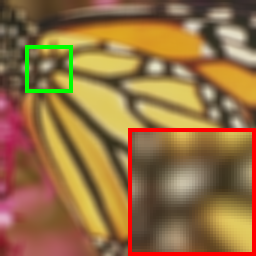
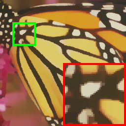
Input	Conv. (Low-Pass)	Total Variation

Figure 1: Illustration of convolution and TV proximity operator for image smoothing. In contrast to a convolution, i.e., a low-pass filter, TV is capable of preserving the edges during smoothing.

3 Approach

Our goal is to incorporate total variation (TV) minimization as a layer into deep-nets. Motivated by the success of TV in classical image restoration, we hypothesize that TV as a layer incorporated into deep-nets is a useful building-block for computer visions tasks. It provides an additional selection of inductive bias over existing layers. Concretely, the input/output dependencies of a TV operation are not achievable by a single convolution layer, as the TV operation is not a linear system. Consider as an example image smoothing: TV can preserve the edges, while a convolution (low-pass filter) blurs the edges as illustrated in Fig. 1. To incorporate this form of inductive bias into deep-nets we develop the differentiable TV layer.

3.1 Differentiable Total Variation Layer

The main component of our TV layer is the proximity operator. For 1D input ${\bm{x}}\in{\mathbb{R}}^{N}$, TV is defined as

$$\text{Prox}_{\text{TV}}^{1D}({\bm{x}},\lambda)=\operatorname*{arg\,min}_{\bm{y}}\frac{1}{2}\left\lVert{\bm{y}}-{\bm{x}}\right\rVert_{2}^{2}+\lambda\left\lVert{\bm{D}}_{N}{\bm{y}}\right\rVert_{1},$$ (1)

where $\left\lVert{\bm{D}}_{N}{\bm{y}}\right\rVert_{1}=\sum_{n}|x_{n+1}-x_{n}|$ and $\lambda\geq 0$. The differencing matrix ${\bm{D}}_{N}$ contains minus ones on its diagonal and an off-diagonal of ones, capturing the gradients of ${\bm{y}}$.

Similarly, the 2D TV (anisotropic) proximity operation for a 2D input ${\bm{X}}$ and output ${\bm{Y}}\in{\mathbb{R}}^{M\times N}$ is defined as:

$$\text{Prox}_{\text{TV}}^{2D}({\bm{X}},\lambda)=\operatorname*{arg\,min}_{\bm{Y}}\frac{1}{2}\left\lVert{\bm{Y}}-{\bm{X}}\right\rVert_{F}^{2}$$ (2)

$$+\lambda\left(\sum_{m}\left\lVert{\bm{D}}_{M}{\bm{Y}}_{\tt row(m)}\right\rVert_{1}+\sum_{n}\left\lVert{\bm{D}}_{N}{\bm{Y}}_{\tt col(n)}\right\rVert_{1}\right),$$

where ${\bm{D}}_{M}$ and ${\bm{D}}_{N}$ denote the corresponding row and column differencing matrix. We incorporate this TV proximity operator as a layer into deep-nets and refer to it as the differentiable total variation layer.

Differentiable TV Layer. Given an input feature map ${\bm{\mathsfit{X}}}\in{\mathbb{R}}^{C\times H\times W}$ the TV layer outputs a tensor ${\bm{\mathsfit{Y}}}$ of the same size. This layer computes the TV-proximity operator independently on each of the channels. The trainable parameters of this layer are $\tilde{\bm{\lambda}}\in{\mathbb{R}}^{C}$ which are used in a SoftPlus [26] non-linearity to guarantee that $\bm{\lambda}$ contains positive numbers which are passed to the proximity operator. The forward operation is hence summarized as: $\forall c\in\{1,\dots,C\}$

$${\bm{\mathsfit{Y}}}_{c}=\text{Prox}_{\text{TV}}^{2D}({\bm{\mathsfit{X}}}_{c},\bm{\lambda}_{c})\;\;\text{where}\;\;\bm{\lambda}_{c}=\text{SoftPlus}(\tilde{\bm{\lambda}}_{c}).$$ (3)

This layer performs smoothing while preserving edges. Note, depending on the desired spatial mode, the layer can also process the rows/columns independently, i.e., a 1D TV-proximity operator per row or column.

In addition, we further extend the capability of this layer, by designing a “sharpening” mode. Inspired by image sharpening techniques, we compute the difference between the input and the smoothed TV output. This difference is added back to the original image to perform “sharpening,” i.e., $\forall c$

$${\bm{\mathsfit{Y}}}_{c} = 2{\bm{\mathsfit{X}}}_{c}-\text{Prox}_{\text{TV}}^{2D}({\bm{\mathsfit{X}}}_{c},\bm{\lambda}_{c}).$$ (4)

The overall pseudo-code of this layer is shown in Fig. 2.

⬇

class TVLayer(Module):

def __init__(self, num_chan, is_sharp):

# num_chan: Number of channels

# is_sharp: Sharpen or not.

self.is_sharp = is_sharp

self._lmbd = Parameters(zeros(num_chan))

def forward(self, x):

# x: Tensor (num_chan, height, width)

lmbd = softplus(self._lmbd)

# Apply batched per channel prox. tv

y = tv_prox_2d(x, lmbd)

if self.is_sharp:

y = 2*x-y

return y

Figure 2: Pseudo code of the proposed TV Layer.

Trainable $\bm{\lambda}$ in TV Layer. Note, a TV Layer with trainable $\bm{\lambda}$ increases a model’s capacity. When $\bm{\lambda}=0$, this layer is an identity function for both smoothing and sharpening as

$${\bm{x}}=\operatorname*{arg\,min}_{\bm{y}}\frac{1}{2}\left\lVert{\bm{y}}-{\bm{x}}\right\rVert_{2}^{2}+0,$$ (5)

and as $2{\bm{x}}-{\bm{x}}={\bm{x}}$ in the sharpening mode. Hence, a network with TV layers and $\bm{\lambda}=0$ is equivalent to a model without this layer. The network can hence learn to “turn-off” this layer if this improves results, avoiding the need to hand-tune $\bm{\lambda}$ when adding the TV layer to a new deep-net architecture. We will now discuss details on how to develop a fast implementation of this TV layer.

3.2 Efficient Implementation

Existing packages that support the TV proximity operator are either generic or lack GPU support. For example, CVXPYLayers uses a generic solver, which is relatively slow compared to specialized TV solvers. In contrast, efficient solvers are fast on the CPU, e.g., the ProxTV toolbox [38, 9], however CPU implementations are not suitable for integration with deep-nets when all other operations occur on the GPU, as memory transfer between GPU and CPU is needed at each layer, making training and inference slow.

To address these short-comings, we develop a GPU-based Projected-Newton [13] method for solving TV by writing custom CUDA kernels. We carefully consider the structure of the TV problem. These custom CUDA kernels are wrapped into PyTorch [53] and can be conveniently called through Python. We will discuss the forward and backward operation for 1D input next.

Forward Operation. Projected-Newton solves the TV-proximity problem (Eq. (1)) via its dual:

$$\max_{{\bm{u}}}\underbrace{-\frac{1}{2}\left\lVert{\bm{D}}_{N}^{\intercal}{\bm{u}}\right\rVert_{2}^{2}+{\bm{u}}^{\intercal}{\bm{D}}_{N}{\bm{x}}}_{\phi({\bm{u}})}~{}~{}~{}\text{s.t.}~{}\left\lVert{\bm{u}}\right\rVert_{\infty}<\lambda.$$ (6)

Specifically, projected-Newton iteratively solves a local quadratic approximation of the objective before performing an update step with a suitable step-size, e.g., following the Armijo rule. Given Eq. (6), the quadratic approximation boils down to solving the linear system

$${\bm{H}}_{\cal S}{\bm{d}}_{\cal S}=\nabla\phi({\bm{u}})_{\cal S},$$ (7)

for ${\bm{d}}_{\cal S}$ which denotes the dual variable update direction. Here, ${\bm{H}}=\nabla^{2}\phi({\bm{u}})$ refers to the Hessian matrix, ${\mathcal{S}}$ refers to the set of indices of active variables and the subscript denotes selecting the rows/columns to form a system based on a subset of the variables.

At a glance, solving Eq. (7) seems expensive. However, note that ${\bm{H}}={\bm{D}}_{N}{\bm{D}}_{N}^{\intercal}$ is a tridiagonal and symmetric matrix. Tridiagonal systems can be solved efficiently by first computing a Cholesky factorization and then solving with backward substitution. Both operations can be performed in linear time, i.e., ${{\mathcal{O}}}(N)$ [74]. Without exploiting this structure, general Gaussian elimination has ${{\mathcal{O}}}(N^{3})$ complexity.

Unfortunately, specialized routines for sub-indexing and solving tridiagonal systems are neither supported by cuBLAS nor by ATen. To enable efficient computation with batching support on the GPU, we implemented 21 custom CUDA kernels. These CUDA operations are integrated with PyTorch for ease of use. We note that these implementations are necessary due to the special structures of the matrices. To give an example, a $N\times N$ tridiagonal matrix can be efficiently stored in a $3\times N$ matrix, storing the diagonal and two off-diagonals. However, this indexing scheme needs to be supported and is not readily available in existing packages.

Next, to select a suitable step-size for direction ${\bm{d}}_{\cal S}$, we use the quadratic interpolation backtracking strategy [51]. We have also implemented a parallelized search strategy, which considers multiple step-sizes of halving intervals in parallel. In practice, we found backtracking to be more efficient as it only iterates a few times.

Backward Operation. To use $\text{Prox}_{\text{TV}}^{1D}({\bm{x}},\lambda)$ as a layer, we need to compute the Jacobian with respect to (w.r.t.) ${\bm{x}}$ and $\lambda$: For readability, we let ${\bm{y}}=\text{Prox}_{\text{TV}}^{1D}$, which yields

$$\frac{\partial{\bm{y}}}{\partial{\bm{x}}}={\bm{M}}{\bm{L}}_{:,\bar{\mathcal{S}}}^{\intercal}~{}~{}\text{and}~{}~{}\frac{\partial{\bm{y}}}{\partial\lambda}=-{\bm{M}}\text{Sign}({\bm{D}}_{N}{\bm{y}})_{\bar{\mathcal{S}}},$$ (8)

where

$${\bm{M}}={\bm{L}}_{:,\bar{\mathcal{S}}}({\bm{L}}_{:,\bar{\mathcal{S}}}^{\intercal}{\bm{L}}_{:,\bar{\mathcal{S}}})^{-1}.$$ (9)

Here, $\bar{\mathcal{S}}$ denotes the set of indices of non-zero values in ${\bm{D}}_{N}{\bm{y}}$, ${\bm{L}}$ denotes a $N\times N$ lower triangular matrix, and the subscript denotes the sub-selection of the column. We refer readers to Cherkaoui et al. [18]’s appendix G.1 for the derivation.

To efficiently compute these Jacobian matrices, observe that ${\bm{L}}_{:,\bar{\mathcal{S}}}^{\intercal}{\bm{L}}_{:,\bar{\mathcal{S}}}$ in Eq. (9) is a positive (semi-definite) matrix. Therefore, we use Cholesky factorization and Cholesky solve to compute the inverse instead of a standard matrix inversion. Again, we implemented custom CUDA kernels to allow for efficient indexing and batching. We integrate this into the backward function of PyTorch to support automatic differentiation.

Algorithm 1 $\text{Prox}_{\text{TV}}^{2D}({\bm{X}},\lambda)$ with Proximal Dykstra Method

  Inputs: ${\bm{X}}$ and $\lambda$

  Initialize: ${\bm{Y}}^{(k)}={\bm{X}}$, ${\bm{P}}_{0}=\mathbf{0}$, ${\bm{Q}}_{0}=\mathbf{0}$

  for $k\in\{1,\ldots,K\}$ do

     for $m\in\{1,\ldots,M\}$ do    # Parallelized with CUDA

        ${\bm{Z}}^{(k)}_{\tt row(m)}=\text{Prox}_{\text{TV}}^{1D}({\bm{Y}}^{(k)}_{\tt row(m)}+{\bm{P}}^{(k)}_{\tt row(m)},\lambda)$

     end for

     ${\bm{P}}^{(k+1)}={\bm{P}}^{(k)}+{\bm{Y}}^{(k)}-{\bm{Z}}^{(k)}$

     for $n\in\{1,\ldots,N\}$ do    # Parallelized with CUDA

        ${\bm{Y}}^{(k+1)}_{\tt col(n)}=\text{Prox}_{\text{TV}}^{1D}({\bm{Z}}^{(k)}_{\tt col(m)}+{\bm{Q}}^{(k)}_{\tt col(n)},\lambda)$

     end for

     ${\bm{Q}}^{(k+1)}={\bm{Q}}^{(k)}+{\bm{Z}}^{(k)}-{\bm{Y}}^{(k+1)}$

  end for

  return  ${\bm{Y}}^{K+1}$

2D TV Proximity. The 2D TV proximity implementation is based on the Proximal Dykstra method [20]. It alternates between solving 1D TV proximity problems for all the rows and columns, i.e.,

$$\min_{\bm{Y}}\frac{1}{2}\left\lVert{\bm{Y}}-{\bm{X}}\right\rVert_{F}^{2} + \lambda\sum_{m}\left\lVert{\bm{D}}_{M}{\bm{Y}}_{\tt row(m)}\right\rVert_{1}$$ (10)

$$\min_{\bm{Y}}\frac{1}{2}\left\lVert{\bm{Y}}-{\bm{X}}\right\rVert_{F}^{2} + \lambda\sum_{n}\left\lVert{\bm{D}}_{N}{\bm{Y}}_{\tt col(n)}\right\rVert_{1}.$$ (11)

Both Eq. (10) and Eq. (11) can be decomposed into 1D TV proximity problems per row or per column. As our 1D TV proximity operator implementation supports batching, we can solve all the rows or all the columns in parallel very efficiently on the GPU. The overall procedure is summarized in Alg. 1. We found three or four iterations of the Proximal Dykstra method to work well in practice. For the backward pass, our TV 1D proximity operator supports automatic differentiation, so back-propagation through Alg. 1 is automatically computed with PyTorch.

Package	Hardware	Forward	Backward	Total
CVXPYLayers	CPU	$20704\pm 32$	$9932\pm 41$	$1770\times$
ProxTV-TS	CPU	$207.8\pm 7.5$	$430.7\pm 7.9$	$37\times$
ProxTV-PN	CPU	$257.3\pm 5.8$	$447.0\pm 9.6$	$41\times$
Ours-PN	Titan X	$9.0\pm 0.7$	$17.7\pm 2.4$	$1.5\times$
Ours-PN	A6000	$10.0\pm 1.5$	$7.3\pm 6.0$	$1\times$

Table 1: Running time (ms) comparison of TV 1D Proximity Operator. We report the total running time relative to Ours-PN on an A6000 GPU.

4 Experiments

First, we compare the running time of TV layers implemented with different approaches. Next, we evaluate the proposed TV layer on a variety of computer vision tasks including: image classification, weakly supervised object localization, edge detection, edge-aware filtering, and image denoising. These tasks cover a wide spectrum of vision applications from high-level semantics understanding to low-level pixel manipulation, demonstrating the practicality of the proposed TV layer. As we are reporting over multiple tasks and metrics, we use $\uparrow$/$\downarrow$ to indicate whether a metric is better when it is higher/lower.

	Noise Type			Blur Type				Corruption Type
Arch.	Gaussian	Shot	Impulse	Glass	Defocus	Motion	Zoom	Snow	Frost	Fog	Brightness	Contrast	Elastic	Pixelate	JPEG	All
AllConv	$36.2$ $\!\pm\!1.4$	$48.9$ $\!\pm\!1.5$	$\bf 46.6$ $\!\pm\!3.1$	$77.9$ $\!\pm\!0.7$	$46.7$ $\!\pm\!2.3$	$72.8$ $\!\pm\!0.5$	$71.9$ $\!\pm\!1.1$	$77.8$ $\!\pm\!0.1$	$71.9$ $\!\pm\!0.8$	$82.5$ $\!\pm\!0.4$	$91.6$ $\!\pm\!0.2$	$67.1$ $\!\pm\!0.9$	$\bf 82.2$ $\!\pm\!0.7$	$72.2$ $\!\pm\!0.5$	$\bf 79.0$ $\!\pm\!0.3$	$68.4$ $\!\pm\!0.5$
TV-Smooth	$\bf 42.7$ $\!\pm\!2.4$	$\bf 55.0$ $\!\pm\!1.4$	$44.8$ $\!\pm\!3.2$	$79.4$ $\!\pm\!0.7$	$49.2$ $\!\pm\!2.5$	$74.5$ $\!\pm\!0.8$	$\bf 74.3$ $\!\pm\!1.2$	$79.4$ $\!\pm\!0.8$	$\bf 75.3$ $\!\pm\!1.1$	$85.0$ $\!\pm\!0.3$	$92.1$ $\!\pm\!0.1$	$69.4$ $\!\pm\!1.1$	$81.8$ $\!\pm\!0.3$	$\bf 73.0$ $\!\pm\!0.6$	$78.4$ $\!\pm\!0.2$	$70.3$ $\!\pm\!0.6$
TV-Sharp	$40.6$ $\!\pm\!1.4$	$53.1$ $\!\pm\!1.5$	$46.5$ $\!\pm\!1.0$	$\bf 79.8$ $\!\pm\!0.3$	$\bf 50.3$ $\!\pm\!0.6$	$\bf 75.7$ $\!\pm\!0.7$	$73.9$ $\!\pm\!0.4$	$\bf 80.3$ $\!\pm\!0.5$	$75.2$ $\!\pm\!0.9$	$\bf 86.2$ $\!\pm\!0.4$	$\bf 92.2$ $\!\pm\!0.1$	$\bf 74.4$ $\!\pm\!0.2$	$81.8$ $\!\pm\!0.3$	$72.6$ $\!\pm\!0.5$	$76.5$ $\!\pm\!0.16$	$\bf 70.6$ $\!\pm\!0.2$

Table 2: Classification accuracy ($\uparrow$) on CIFAR10-C over different types of corruptions.

4.1 Timing Analysis

We compare with a generic TV solver using CVXPYLayers [23, 2] which supports back-propagation. We also compare with specialized TV solvers using the ProxTV toolbox [38, 9] with a PyTorch implementation of the backward pass. Both, CVXPYLayers and ProxTV only support CPU computations.

We time each of these methods on a batch of signals with dimension $256\times 32\times 32$. This is a typical dimension for small scale computer vision tasks. The data contains a unit step signal with additive Gaussian noise and $\lambda$ is set to one. Timing evaluation is done on an NVIDIA TITAN X or A6000 GPU and an Intel Core i7-6700K CPU. We report the mean and standard deviation over 25 runs.

Results. In Tab. 1 we report the forward and backward computation time, in milliseconds, for each of the methods. We observe that ProxTV with specialized solver is faster than CVXPYLayers using a generic solver. We report ProxTV with two different specialized TV solvers, namely, Taut-String (TS) and Projected Newton (PN). However, these CPU based methods remain too slow for practical vision applications, e.g., an entire inference on ResNet101 takes $\sim 150$ ms. With GPU support, our approach achieves a $1770\times$ speedup over CVXPYLayers, and is $37\times$ to $41\times$ faster than ProxTV. This significant speedup enables the scaling of TV layers to real computer vision tasks.

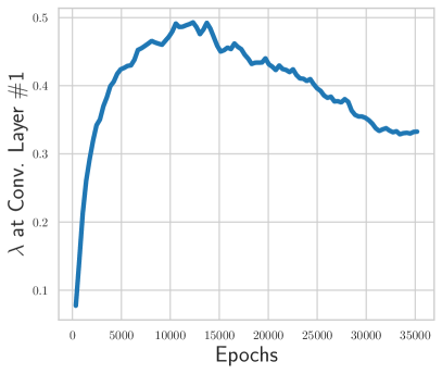
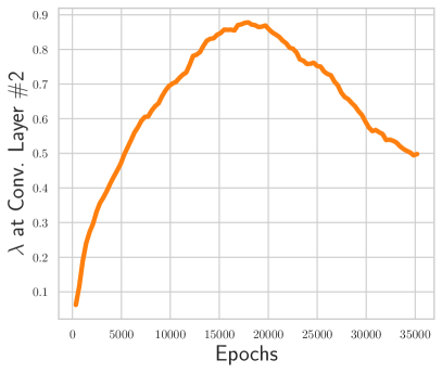
Figure 3: Visualization of $\lambda$ vs. number of training epochs for TV-Sharp at the first and second Conv. block. We observe that $\lambda$ learns to be greater than zero.

4.2 Image Classification

We conduct experiments on CIFAR10 data [42] evaluating two aspects: (a) standard classification and (b) out of domain generalization. We study the effect of the proposed total variation layer on a baseline architecture of an All Convolutional Network [69]. We study both the smoothing and the sharpening TV layer, with $\lambda$ shared across channels, being added in the first three convolution blocks. Specifically, we insert the TV layers before batch-normalization of each block. We refer to these modified architectures as TV-Smooth and TV-Sharp. We initialize $\lambda=0.05$ and train them jointly with the model parameters.

Standard Classification. On CIFAR10, the baseline model AllConvNet achieved an accuracy of $93.51\%\pm 0.18\%$ (standard deviation reported over five runs). With the smoothing and sharpening TV layer added, TV-Smooth and TV-Sharp achieve an accuracy of $93.61\pm 0.17\%$ and $93.43\pm 0.24\%$ respectively. As can be seen, adding these TV layers performs on par with the baseline model.

To ensure that the models actually use the TV modules, we visualize $\lambda$ in Eq. (1), at each layer, throughout training iterations in Fig. 3. Note, $\lambda$ learns to be non-zero, indicating that the TV layers are impacting the model architecture.

Out of Domain Generalization. To further assess how TV modules affect the model, we evaluate out-of-distribution (o.o.d.) generalization using CIFAR10-C data [34]. Models are trained on clean data and evaluated on corrupted data, e.g., noise is added to the images. Classification accuracy on CIFAR10-C are reported in Tab. 2. On average, both the TV-Smooth and TV-Sharp model improve the o.o.d. generalization over the baseline model. We observe: the TV-Smooth model generalizes better to additive noise corruption, whereas TV-Sharp improves the accuracy on blur corruption. These results match our expected behavior of sharpening and smoothing and illustrate that optimization as a layer is a useful way to encode a models’ inductive bias.

Method	VGG-16	Inception-V3	ResNet-50
CAM-paper	60.02	63.40	63.65
CAM-repro.	60.13	63.51	64.09
CAM-repro.+TV (Ours)	60.35	63.80	65.36

Table 3: WSOL localization accuracy, MaxBoxAccV2 ($\uparrow$), on the test set from Choe et al. [19] for ImageNet pre-trained models.

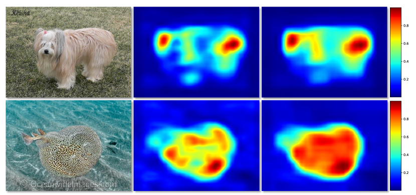
Figure 4: Visualization of WSOL results. We show the input images (left), the heat-maps from CAM (center) and ours (right).

4.3 Weakly Supervised Object Localization

Weakly Supervised Object Localization (WSOL) is a popular interpretability tool in various computer vision tasks. It learns to localize objects with only image-level labels. The seminal work Class Activation Mapping (CAM) [85] first studies WSOL for image classification. Follow-up work [65, 57] further generalizes to broader domains such as vision and language. We believe TV layer is beneficial to WSOL as it aids the localization results, i.e., class-wise heat-maps, to be smoother and better aligned with boundaries.

For evaluation, the most popular method is to infer surrounding bounding boxes of the computed class heat-maps and compare to ground-truth ones. However, recent WSOL analysis work [19] points out that CAM is still the state-of-the-art WSOL method under a fairer evaluation setting. The performance boost achieved in follow-ups are illusory caused by wrong experimental settings and inconsistent bounding box generation methods. We thus adopt both CAM and the fair evaluation protocol in this work and test TV layer on it.

Experimental Setup. We test three different models: VGG-16 [67], ResNet-50 [33], and Inception-V3 [70]. We use a fixed TV2D-Smooth layer shared across all channels with $\lambda=1$. We insert this TV layer right before the CAM layer of each network. We use the code base from Choe et al. [19] who discuss a more fair experimental setting: all WSOL methods are fine-tuned on a fixed validation set to search for the best hyper-parameters and then test on newly collected test images. Since the fine-tuned models are not released, we reproduce using the released code and report both results (CAM-repro. and CAM-paper) for completeness.

Results. We report quantitative metrics in Tab. 3 where we observe that a TV layer consistently improves WSOL results of various models (0.22/0.29/1.27 for VGG-16/Inception-V2/ResNet-50). We further show qualitative comparisons between the vanilla version and ours in Fig. 4 where we observe that the TV layer helps WSOL models to generate smoother and aligned results.

	BIPED [56]			MDBD [50]
Method	ODS ($\uparrow$)	OIS ($\uparrow$)	AP ($\uparrow$)	ODS ($\uparrow$)	OIS ($\uparrow$)	AP($\uparrow$)
HED [78]	.829	.847	.869	.851	.864	.890
RCF [45]	.843	.859	.882	.857	.862	-
DexiNed [56]	.859	.867	.905	.859	.864	.917
DexiNed+TV	.874	.879	.914	.863	.875	.920

Table 4: Quantitative comparison for edge detection on BIPED and MDBD data. Baselines are obtained from corresponding papers.

4.4 Edge Detection

Edge detection is the task of identifying all the edges for a given input image. For learning based methods, this is formulated as a binary classification problem for each pixel location, i.e., classifying whether a given pixel in the image is an edge. The task is illustrated in Fig. 5. We evaluate on the recent BIPED [56] and the Multicue (MBDB) [50] dataset for edge detection.

Experimental Setup. We compare to the Dense extreme inception Network for edge detection (DexiNed) baseline proposed by Poma et al. [56]. DexiNed consists of convolutional blocks and follows a multi-scale and multi-head architecture. Before each stage of max-pooling, DexiNed outputs an edge-map at the scale of $2\times$, $4\times$, $8\times$ and $16\times$. The final edge-map prediction is obtained by averaging the edge-map at each scale. For our model, we added TV2D-Sharp layers, with trainable $\bm{\lambda}$, at the $2\times$, $4\times$ and $8\times$ edge-maps. At the final edge-map, we added a TV2D-Smooth layer.

Evaluation metrics for edge detection [5] are based on the

$$\text{F-measure}=2\cdot\frac{\text{precision}\cdot\text{recall}}{\text{precision}+\text{recall}},$$ (12)

with different thresholds, including: (a) optimal dataset scale (ODS) which corresponds to using the best threshold over a dataset; (b) optimal image scale (OIS) which corresponds to using the best threshold per image and average precision (AP) which is the area under the precision-recall curve.

Results. Following Poma et al. [56], we compared our DexiNed + TV to the standard DexiNed [56], RCF [45] and HED [78] in Tab. 4 using the BIPED and MDBD dataset. All the models are trained only on the BIPED dataset. As can be seen, our approach achieves improvements across ODS, OIS, and AP for both BIPED and MDBD data. A qualitative comparison of the final detected edges is shown in Fig. 5. We observe that DexiNed+TV predicts sharper edges and suppresses textures better than DexiNed.

Input	Ground-Truth
DexiNed [56]	DexiNed+TV (Ours)

Figure 5: Qualitative comparison on edge detection.

Input	Final Conv. Layer	After TV-Smooth

Figure 6: Visualization of the effects of the final TV-smooth layer for edge preserving smoothing.

4.5 Edge Preserving Smoothing

Edge preserving smoothing is the task of smoothing images while maintaining sharp edges. To fairly compare across algorithms,  Zhu et al. [86] propose a dataset (BenchmarkEPS) consisting of 500 training and testing images with corresponding “ground-truth” smoothed images.

Zhu et al. [86] also propose to use two evaluation metrics, Weighted Root Mean Squared Error (WRMSE) and Weighted Mean Absolute Error (WMAE) defined as follows:

$$\small\text{WRMSE}({\bm{I}},\hat{\bm{I}})=\sqrt{\frac{\sum_{n=1}^{N}\sum_{k=1}^{K}w^{(n,k)}\left\lVert\hat{\bm{I}}^{(n)}-{\bm{I}}^{(n,k)}\right\rVert_{2}^{2}}{N\cdot K\cdot H\cdot W}}$$

 and 

$$\small\text{WMAE}({\bm{I}},\hat{\bm{I}})=\frac{\sum_{n=1}^{N}\sum_{k=1}^{K}w^{(n,k)}\left\lVert\hat{\bm{I}}^{(n)}-{\bm{I}}^{(n,k)}\right\rVert_{1}}{N\cdot K\cdot H\cdot W},$$

where ${\bm{I}}^{(n,k)}$ corresponds to the $k$-th ground-truth of the $n$-th image (with height $H$ and width $W$), $\hat{\bm{I}}^{(n)}$ denotes the prediction of the $n$-th image, $w^{(n,k)}$ denotes the normalized weight of the ground-truth. Note, there are multiple ground-truths for each image, hence annotators vote for each ground-truth and their votes are normalized into weight $w^{(n,k)}$.

For evaluation, we compared with two deep-net baselines, VDCNN and ResNet, proposed by Zhu et al. [86], as well as an optimization based approach of L1 smoothing [14]. The ResNet architecture consists of 16 Residual Blocks followed by three convolutional layers with a skip connection from the input. For our model (ResNetTV), we insert four TV1D-Sharp layers with alternating row/column directions into the Residual Blocks and lastly a TV2D-Smooth layer (with shared $\lambda$ across channels) after the last skip connection. This design is due to the observations that residual blocks learn high-frequency content and the final output is smooth.

Method	WRMSE ($\downarrow$)	WMAE ($\downarrow$)
L1 smooth [14]	9.89	5.76
VDCNN [86]	9.78	6.15
ResNet [86]	9.03	5.55
ResNetTV (Ours)	8.87	5.47

Table 5: Quantitative results on the edge-preserving image smoothing benchmark [86].

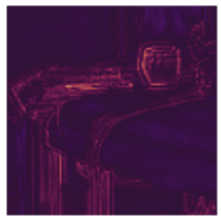
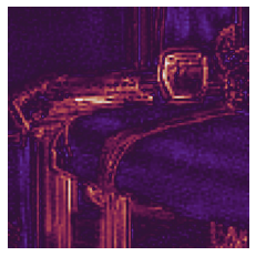
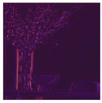
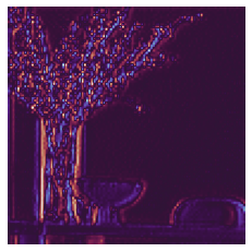
Input	Feature	After TV-Sharp

Figure 7: Visualization of feature maps before and after TV-Sharp layer at a residual block on ResNetTV. The red box indicates the region of visualized (zoomed-in) feature maps.

Results. In Tab. 5, we report the quantitative results. We observe improvements in both WRMSE and WMAE over the baselines, both the pure optimization based method and deep learning methods. This demonstrates the benefits of incorporating optimization as a layer into deep-nets. Beyond the quantitative improvements, we analyze the effect of the final TV-Smooth layer, which can be easily visualized as it is operating in the image space. First, we observe that the learned $\lambda=15.1$, which means that the layer is indeed performing smoothing. To illustrate its effect, in Fig. 6 we visualize the image at the final convolutional layer and after the TV-Smooth layer. As can be seen, the image at the final convolutional layer (column 2 of Fig. 6) is already smoothed by a decent amount. The final TV-Smooth layer further filters the image while preserving the edges which improves the result. We suspect that addition of the TV-Smooth layer aids the overall performance as the deep-net does not need to use its capacity for part of the smoothing procedure.

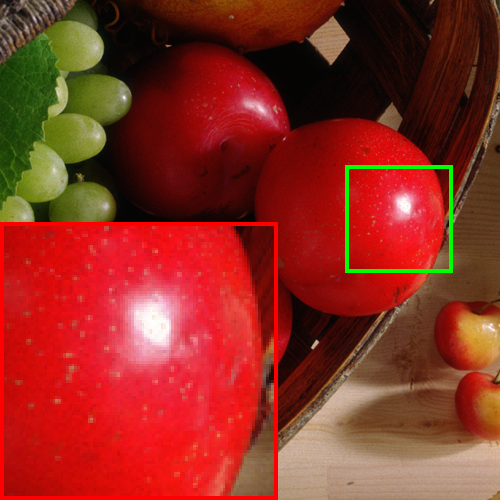
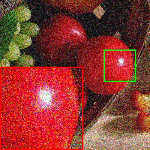
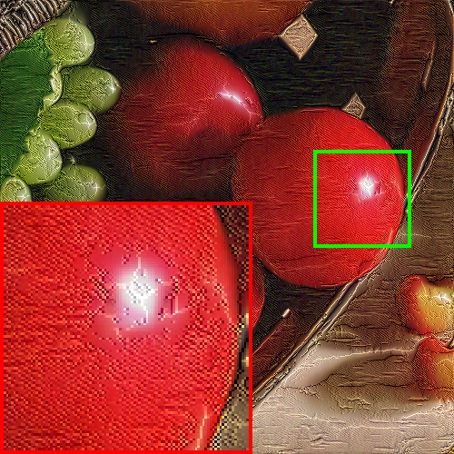
Ground-Truth	Noisy Input	After Input TV	Final Residual Block	After Output TV

Figure 8: Visualizing the effects of the input and output TV layers (see Eq. (14)) on image denoising.

We also analyze the effect of the TV layer on the feature maps. In Fig. 7 we show an intermediate feature map before and after a TV-Sharp layer. As expected, feature maps are sharpened, leading to more prominent edges in feature space. While it is difficult to directly interpret these features maps, intuitively, a deep-net that performs well on edge preserving smoothing should easily capture edges of an image.

4.6 Image Denoising

Image denoising is the task of recovering a clean image given a noisy input image. Deep-net-based approaches typically formulate image denoising as a regression task, i.e., regress to the clean RGB values given a noisy input. We consider color images corrupted by additive white Gaussian noise and report the average peak signal-to-noise ratio (PSNR) [36]; the higher the better. We evaluate on the common CBSD68 [49], Kodak24 [27] and McMaster [83] data.

We use DnCNN [82] as our base model. It consists of residual blocks with a full skip connect from the input, i.e.,

$$\text{DnCNN}({\bm{I}})\triangleq{\mathcal{R}}({\bm{I}})+{\bm{I}},$$ (13)

where ${\mathcal{R}}$ denotes the residual blocks and ${\bm{I}}$ is the noisy input image. We added TV2D-Smooth layers at the input and output of the network, i.e.,

$$\text{DnCNNTV}({\bm{I}})\triangleq\text{Prox}_{\text{TV}}^{2D}\left(\left[{\mathcal{R}}(\tilde{\bm{I}})+\tilde{\bm{I}}\right],\bm{\lambda}_{\tt out}\right),$$ (14)

where $\tilde{\bm{I}}\triangleq\text{Prox}_{\text{TV}}^{2D}({\bm{I}},\bm{\lambda}_{\tt in})$. We use the KAIR toolbox to train these denoising models.

Results. In Tab. 6, we report the average PSNR over different noise-levels. We observe a larger gain on the $\sigma=50$ setting and on the McMaster dataset. We further analyze the behavior of the two added TV layers. As the TV layers are added on the image space, we can directly visualize them. In Fig. 8 we visualize the noisy input image, the image immediately after the input TV layer, the final residual block, and the final result after the output TV layer. We observe: the input TV layer performs a very weak noise reduction, see column two vs. three in Fig. 8. Next, in column four, we observe: the residual block outputs an image with sharp edges but with high-frequency artifacts. These artifacts are then smoothed by the final output TV layer (see col. five).

Limitations. We note that our result is not the state-of-the-art model, i.e., SwinTransformer [44]. We have also added TV layers to SwinTransformer models. However, $\bm{\lambda}$s learn to be zero which effectively turns the TV layer off. We suspect that the TV smoothing layer leads to overly smooth output. Hence, when a deep-net has enough capacity the TV layer may learn to use $\bm{\lambda}=0$ to avoid smoothing.

Method	CBSD68 [49]		Kodak24 [27]		McMaster [83]
Noise-level $\sigma$	25	50	25	50	25	50
DnCNN [82]	31.24	27.95	32.14	28.95	31.52	28.62
DnCNNTV	31.26	28.07	32.15	29.09	32.32	29.35

Table 6: Quantitative comparison for image denoising. We report the average PSNR ($\uparrow$) for each of the methods.

5 Conclusion

Optimization as a layer is a promising direction to incorporate inductive bias into deep-nets. In this work, we propose to include total variation minimization as a layer. Our method achieves $37\times$ speedup over existing solutions scaling TV layers to real computer vision tasks. On five tasks, we demonstrate existing deep-net architectures can benefit from use of TV-layers. We believe the TV layer is an important building block for deep learning in computer vision and foresee more applications to benefit from it.

Acknowledgements: This work is supported in part by NSF #1718221, 2008387, 2045586, 2106825, MRI #1725729, NIFA 2020-67021-32799 and Cisco Systems Inc. (CG 1377144 - thanks for access to Arcetri).

References

- Afonso et al. [2010] Manya V. Afonso, José M. Bioucas-Dias, and Mário A.T. Figueiredo. An augmented lagrangian approach to the constrained optimization formulation of imaging inverse problems. IEEE TIP, 2010.
- Agrawal et al. [2019] Akshay Agrawal, Brandon Amos, Shane Barratt, Stephen Boyd, Steven Diamond, and J. Zico Kolter. Differentiable convex optimization layers. In Proc. NeurIPS, 2019.
- Amos et al. [2018] Brandon Amos, Ivan Jimenez, Jacob Sacks, Byron Boots, and J. Zico Kolter. Differentiable MPC for end-to-end planning and control. In Proc. NeurIPS, 2018.
- Amos and Kolter [2017] Brandon Amos and J. Zico Kolter. OptNet: differentiable optimization as a layer in neural networks. In Proc. ICML, 2017.
- Arbelaez et al. [2010] Pablo Arbelaez, Michael Maire, Charless Fowlkes, and Jitendra Malik. Contour detection and hierarchical image segmentation. IEEE TPAMI, 2010.
- Aujol et al. [2006] Jean-François Aujol, Guy Gilboa, Tony Chan, and Stanley Osher. Structure-texture image decomposition—modeling, algorithms, and parameter selection. IJCV, 2006.
- Bai et al. [2019] Shaojie Bai, J. Zico Kolter, and Vladlen Koltun. Deep equilibrium models. In Proc. NeurIPS, 2019.
- Bai et al. [2020] Shaojie Bai, Vladlen Koltun, and J. Zico Kolter. Multiscale deep equilibrium models. In Proc. NeurIPS, 2020.
- Barbero and Sra [2018] Alvaro Barbero and Suvrit Sra. Modular proximal optimization for multidimensional total-variation regularization. JMLR, 2018.
- Barratt and Boyd [2021] Shane T Barratt and Stephen P Boyd. Least squares auto-tuning. Engineering Optimization, 2021.
- Beck and Teboulle [2009] Amir Beck and Marc Teboulle. Fast gradient-based algorithms for constrained total variation image denoising and deblurring problems. IEEE TIP, 2009.
- Belanger and McCallum [2016] David Belanger and Andrew McCallum. Structured prediction energy networks. In Proc. ICML, 2016.
- Bertsekas [1982] Dimitri P Bertsekas. Projected Newton methods for optimization problems with simple constraints. SICON, 1982.
- Bi et al. [2015] Sai Bi, Xiaoguang Han, and Yizhou Yu. An L1 image transform for edge-preserving smoothing and scene-level intrinsic decomposition. ACM TOG, 2015.
- Borgerding et al. [2017] Mark Borgerding, Philip Schniter, and Sundeep Rangan. AMP-inspired deep networks for sparse linear inverse problems. IEEE TSP, 2017.
- Chambolle [2004] Antonin Chambolle. An algorithm for total variation minimization and applications. JMIV, 2004.
- Chan and Wong [1998] Tony F Chan and Chiu-Kwong Wong. Total variation blind deconvolution. IEEE TIP, 1998.
- Cherkaoui et al. [2020] Hamza Cherkaoui, Jeremias Sulam, and Thomas Moreau. Learning to solve TV regularised problems with unrolled algorithms. In Proc. NeurIPS, 2020.
- Choe et al. [2020] Junsuk Choe, Seong Joon Oh, Seungho Lee, Sanghyuk Chun, Zeynep Akata, and Hyunjung Shim. Evaluating weakly supervised object localization methods right. In Proc. CVPR, 2020.
- Combettes and Pesquet [2011] Patrick L. Combettes and Jean-Christophe Pesquet. Proximal splitting methods in signal processing. In Fixed-point algorithms for inverse problems in science and engineering. 2011.
- Combettes and Wajs [2005] Patrick L. Combettes and Valérie R Wajs. Signal recovery by proximal forward-backward splitting. Multiscale Modeling & Simulation, 2005.
- Condat [2013] Laurent Condat. A direct algorithm for 1-d total variation denoising. IEEE SPL, 2013.
- Diamond and Boyd [2016] Steven Diamond and Stephen Boyd. CVXPY: A Python-embedded modeling language for convex optimization. JMLR, 2016.
- Domke [2012] Justin Domke. Generic methods for optimization-based modeling. In Proc. AISTATS, 2012.
- Donoser et al. [2009] Michael Donoser, Martin Urschler, Martin Hirzer, and Horst Bischof. Saliency driven total variation segmentation. In Proc. ICCV, 2009.
- Dugas et al. [2001] Charles Dugas, Yoshua Bengio, François Bélisle, Claude Nadeau, and René Garcia. Incorporating second-order functional knowledge for better option pricing. In Proc. NeurIPS, 2001.
- Franzen [1999] Rich Franzen. Kodak lossless true color image suite. source: http://r0k. us/graphics/kodak, 1999.
- Fukushima [1980] Kunihiko Fukushima. Neocognitron: A self-organizing neural network model for a mechanism of pattern recognition unaffected by shift in position. Biological Cybernetics, 1980.
- Gould et al. [2021] Stephen Gould, Richard Hartley, and Dylan John Campbell. Deep declarative networks. IEEE TPAMI, 2021.
- Graber et al. [2018] Colin Graber, Ofer Meshi, and Alexander G. Schwing. Deep Structured Prediction with Nonlinear Output Transformations. In Proc. NeurIPS, 2018.
- Graber and Schwing [2019] Colin Graber and Alexander G. Schwing. Graph structured prediction energy networks. In Proc. NeurIPS, 2019.
- Gregor and LeCun [2010] Karol Gregor and Yann LeCun. Learning fast approximations of sparse coding. In Proc. ICML, 2010.
- He et al. [2016] Kaiming He, Xiangyu Zhang, Shaoqing Ren, and Jian Sun. Deep residual learning for image recognition. In Proc. CVPR, 2016.
- Hendrycks and Dietterich [2019] Dan Hendrycks and Thomas Dietterich. Benchmarking neural network robustness to common corruptions and perturbations. In Proc. ICLR, 2019.
- Hochreiter and Schmidhuber [1997] Sepp Hochreiter and Jürgen Schmidhuber. Long short-term memory. Neural Computation, 1997.
- Hore and Ziou [2010] Alain Hore and Djemel Ziou. Image quality metrics: PSNR vs. SSIM. In Proc. ICPR, 2010.
- Ioffe and Szegedy [2015] Sergey Ioffe and Christian Szegedy. Batch normalization: Accelerating deep network training by reducing internal covariate shift. In Proc. ICML, 2015.
- Jiménez and Sra [2011] Álvaro Barbero Jiménez and Suvrit Sra. Fast Newton-type methods for total variation regularization. In ICML, 2011.
- Joachims et al. [2009] Thorsten Joachims, Thomas Finley, and Chun-Nam John Yu. Cutting-plane training of structural SVMs. Machine learning, 2009.
- Johnson et al. [2016] Justin Johnson, Alexandre Alahi, and Li Fei-Fei. Perceptual losses for real-time style transfer and super-resolution. In Proc. ECCV, 2016.
- Kipf and Welling [2017] Thomas N. Kipf and Max Welling. Semi-supervised classification with graph convolutional networks. In Proc. ICLR, 2017.
- Krizhevsky et al. [2009] Alex Krizhevsky, Geoffrey Hinton, et al. Learning multiple layers of features from tiny images. 2009.
- LeCun et al. [1999] Yann LeCun, Patrick Haffner, Léon Bottou, and Yoshua Bengio. Object recognition with gradient-based learning. In Shape, contour and grouping in computer vision. 1999.
- Liang et al. [2021] Jingyun Liang, Jiezhang Cao, Guolei Sun, Kai Zhang, Luc Van Gool, and Radu Timofte. SwinIR: Image restoration using SWIN transformer. In Proc. ICCVW, 2021.
- Liu et al. [2017] Yun Liu, Ming-Ming Cheng, Xiaowei Hu, Kai Wang, and Xiang Bai. Richer convolutional features for edge detection. In Proc. CVPR, 2017.
- Liu et al. [2017] Ziwei Liu, Raymond A. Yeh, Xiaoou Tang, Yiming Liu, and Aseem Agarwala. Video frame synthesis using deep voxel flow. In Proc. ICCV, 2017.
- Mahendran and Vedaldi [2015] Aravindh Mahendran and Andrea Vedaldi. Understanding deep image representations by inverting them. In Proc. CVPR, 2015.
- Marquina and Osher [2008] Antonio Marquina and Stanley J Osher. Image super-resolution by TV-regularization and bregman iteration. Journal of Scientific Computing, 2008.
- Martin et al. [2001] David Martin, Charless Fowlkes, Doron Tal, and Jitendra Malik. A database of human segmented natural images and its application to evaluating segmentation algorithms and measuring ecological statistics. In Proc. ICCV, 2001.
- Mély et al. [2016] David A. Mély, Junkyung Kim, Mason McGill, Yuliang Guo, and Thomas Serre. A systematic comparison between visual cues for boundary detection. Vis. Res., 2016.
- Nocedal [2006] Jorge. Nocedal. Numerical Optimization. Springer New York, 2nd ed. edition, 2006.
- Osher et al. [2005] Stanley Osher, Martin Burger, Donald Goldfarb, Jinjun Xu, and Wotao Yin. An iterative regularization method for total variation-based image restoration. Multiscale Modeling & Simulation, 2005.
- Paszke et al. [2019] Adam Paszke, Sam Gross, Francisco Massa, Adam Lerer, James Bradbury, Gregory Chanan, Trevor Killeen, Zeming Lin, Natalia Gimelshein, Luca Antiga, and et al. Pytorch: An imperative style, high-performance deep learning library. In Proc. NeurIPS, 2019.
- Perrone and Favaro [2014] Daniele Perrone and Paolo Favaro. Total variation blind deconvolution: The devil is in the details. In Proc. CVPR, 2014.
- Pogančić et al. [2020] Marin Vlastelica Pogančić, Anselm Paulus, Vit Musil, Georg Martius, and Michal Rolinek. Differentiation of blackbox combinatorial solvers. In Proc. ICLR, 2020.
- Poma et al. [2020] Xavier Soria Poma, Edgar Riba, and Angel Sappa. Dense extreme inception network: Towards a robust CNN model for edge detection. In Proc. WACV, 2020.
- Ren et al. [2021] Zhongzheng Ren, Ishan Misra, Alexander G. Schwing, and Rohit Girdhar. 3d spatial recognition without spatially labeled 3d. In Proc. CVPR, 2021.
- Ren et al. [2020] Zhongzheng Ren, Raymond A. Yeh, and Alexander Schwing. Not all unlabeled data are equal: Learning to weight data in semi-supervised learning. In Proc. NeurIPS, 2020.
- Rockafellar [1976] R Tyrrell Rockafellar. Monotone operators and the proximal point algorithm. SICON, 1976.
- Rolínek et al. [2020] Michal Rolínek, Vít Musil, Anselm Paulus, Marin Vlastelica, Claudio Michaelis, and Georg Martius. Optimizing rank-based metrics with blackbox differentiation. In Proc. CVPR, 2020.
- Rolínek et al. [2020] Michal Rolínek, Paul Swoboda, Dominik Zietlow, Anselm Paulus, Vít Musil, and Georg Martius. Deep graph matching via blackbox differentiation of combinatorial solvers. In Proc. ECCV, 2020.
- Rudin et al. [1992] Leonid I Rudin, Stanley Osher, and Emad Fatemi. Nonlinear total variation based noise removal algorithms. Physica D: nonlinear phenomena, 1992.
- Rumelhart et al. [1986] David E. Rumelhart, Geoffrey E Hinton, and Ronald J Williams. Learning representations by back-propagating errors. Nature, 1986.
- Scarselli et al. [2008] Franco Scarselli, Marco Gori, Ah Chung Tsoi, Markus Hagenbuchner, and Gabriele Monfardini. The graph neural network model. IEEE TNNLS, 2008.
- Selvaraju et al. [2017] Ramprasaath R. Selvaraju, Michael Cogswell, Abhishek Das, Ramakrishna Vedantam, Devi Parikh, and Dhruv Batra. Grad-cam: Visual explanations from deep networks via gradient-based localization. In Proc. ICCV, 2017.
- Shen and Chan [2002] Jianhong Shen and Tony F. Chan. Mathematical models for local nontexture inpaintings. SIAP, 2002.
- Simonyan and Zisserman [2015] Karen Simonyan and Andrew Zisserman. Very deep convolutional networks for large-scale image recognition. In Proc. ICLR, 2015.
- Sprechmann et al. [2012] Pablo Sprechmann, Alex Bronstein, and Guillermo Sapiro. Learning efficient structured sparse models. In Proc. ICML, 2012.
- Springenberg et al. [2014] Jost Tobias Springenberg, Alexey Dosovitskiy, Thomas Brox, and Martin Riedmiller. Striving for simplicity: The all convolutional net. arXiv preprint arXiv:1412.6806, 2014.
- Szegedy et al. [2016] Christian Szegedy, Vincent Vanhoucke, Sergey Ioffe, Jon Shlens, and Zbigniew Wojna. Rethinking the inception architecture for computer vision. In Proc. CVPR, 2016.
- Taskar et al. [2004] Ben Taskar, Carlos Guestrin, and Daphne Koller. Max-margin markov networks. In Proc. NeurIPS, 2004.
- Teed and Deng [2021] Zachary Teed and Jia Deng. RAFT-3D: Scene flow using rigid-motion embeddings. In Proc. CVPR, 2021.
- Tsochantaridis et al. [2005] Ioannis Tsochantaridis, Thorsten Joachims, Thomas Hofmann, Yasemin Altun, and Yoram Singer. Large margin methods for structured and interdependent output variables. JMLR, 2005.
- Van Loan [2000] Charles F. Van Loan. Introduction to scientific computing : a matrix-vector approach using MATLAB. 2000.
- Vaswani et al. [2017] Ashish Vaswani, Noam Shazeer, Niki Parmar, Jakob Uszkoreit, Llion Jones, Aidan N Gomez, Łukasz Kaiser, and Illia Polosukhin. Attention is all you need. In Proc. NeurIPS, 2017.
- Wang et al. [2019] Po-Wei Wang, Priya Donti, Bryan Wilder, and J. Zico Kolter. SATNet: Bridging deep learning and logical reasoning using a differentiable satisfiability solver. In Proc. ICML, 2019.
- Wu and He [2018] Yuxin Wu and Kaiming He. Group normalization. In Proc. ECCV, 2018.
- Xie and Tu [2015] Saining Xie and Zhuowen Tu. Holistically-nested edge detection. In Proc. CVPR, 2015.
- Yeh et al. [2017] Raymond A. Yeh, Chen Chen, Teck Yian Lim, Alexander G Schwing, Mark Hasegawa-Johnson, and Minh N Do. Semantic image inpainting with deep generative models. In Proc. CVPR, 2017.
- Yeh et al. [2019] Raymond A. Yeh, Yuan-Ting Hu, and Alexander G. Schwing. Chirality nets for human pose regression. In Proc. NeurIPS, 2019.
- Yeh et al. [2017] Raymond A. Yeh, Jinjun Xiong, Wen-Mei Hwu, Minh Do, and Alexander G. Schwing. Interpretable and globally optimal prediction for textual grounding using image concepts. Proc. NeurIPS, 2017.
- Zhang et al. [2017] Kai Zhang, Wangmeng Zuo, Yunjin Chen, Deyu Meng, and Lei Zhang. Beyond a gaussian denoiser: Residual learning of deep cnn for image denoising. IEEE TIP, 2017.
- Zhang et al. [2011] Lei Zhang, Xiaolin Wu, Antoni Buades, and Xin Li. Color demosaicking by local directional interpolation and nonlocal adaptive thresholding. JEI, 2011.
- Zhang et al. [2017] Zhifei Zhang, Yang Song, and Hairong Qi. Age progression/regression by conditional adversarial autoencoder. In Proc. CVPR, 2017.
- Zhou et al. [2016] Bolei Zhou, Aditya Khosla, Agata Lapedriza, Aude Oliva, and Antonio Torralba. Learning deep features for discriminative localization. In Proc. CVPR, 2016.
- Zhu et al. [2019] Feida Zhu, Zhetong Liang, Xixi Jia, Lei Zhang, and Yizhou Yu. A benchmark for edge-preserving image smoothing. IEEE TIP, 2019.