On the origin of matter-antimatter asymmetry in the Universe

Abstract

In order to investigate the origin of matter-antimatter asymmetry in the Universe, we adopt a theoretical framework where the standard model emerges as a Poincaré invariant field theory localized at a domain-antidomain wall (DW-aDW) brane pair of a theory which lives on a higher dimensional bulk. We argue that such a system of a parallel DW-aDW pair could have been created at a very early epoch of the cosmological evolution when the Universe was still of microscopic size because its creation is topologically possible as compared to a single DW creation when the perpendicular extra dimension is compact. The conservation laws, such as of charge and chirality, are not violated in vacuum fluctuations of the combined DW-aDW system, but as we show their simultaneous conservation for each wall separately may not be favorable in certain processes. In particular, as expansion of spacetime occurs in the higher dimensional bulk, the distance $d$ between the DW and the aDW increases as a function of time. We show that during the early stages of the cosmological evolution, when $d$ was of microscopic size, the leading mechanism for pair-creation from fluctuations of the gauge-field with polarization perpendicular to the DWs (i.e., polarization along the extra dimension) was one in which the particle and the antiparticle were created on the opposite domain-walls hosting opposite chirality fermions. This mechanism allows for a matter-antimatter asymmetry to appear separately in the DW and the aDW, while in the combined DW-aDW system no such asymmetry was allowed. In this scenario, at a later and the present stage of the cosmological evolution, where $d$ is macroscopically large, the probability to violate these conservation laws on a single DW, as a function of the inter-wall distance, is exponentially suppressed.

organization=Department of Physics, Florida State University and
Department of Physics, National and Kapodistrian University of Athens, Panepistimioupolis, Zografos, 157 84 Athens, Greece, city=Tallahassee, post=32306-4350, state=Florida, country=USA

1 Introduction

The idea of using additional dimensions dates back to the early works of Kaluza[1] and Klein[2], who tried to unify electromagnetism with gravity by means of a theory with a compact fifth dimension. During the last two decades, the main attempts to use extra dimensions aim at incorporating gravity and gauge interactions in a unique scheme in a reliable manner. Extra dimensions is a fundamental aspect of string theory[3, 4, 5] which is consistently formulated only in a space-time of more than four dimensions. For some time, however, it was conventional to assume that such extra dimensions were compactified to manifolds of small radii, with sizes about the order of the Planck length, $l_{P}\sim 10^{-33}$ cm, such that they would remain hidden to the experiment, thus, justifying why we see only four dimensions[6]. In this picture, it was believed that the relevant energy scale where quantum gravity and string effects would become important is Planck’s mass $M_{P}c^{2}$ from where Planck’s length is defined as $l_{P}=\hbar/(M_{P}c)$. Later studies of the E${}_{8}\times$E₈ heterotic string by Witten[7] and Horava and Witten[8, 9] includes a systematic analysis of eleven-dimensional supergravity on a manifold with boundary believed to be relevant to this heterotic string. These studies suggest that some, if not all, of the extra dimensions could be larger than the Planck length scale. String theory constructions include D-branes in which, while gravity can be free to propagate in extra dimensions, the standard model (SM) fields are confined to branes. For example Arkani-Hamed, Dimopoulos and Dvali[10] (ADD) have introduced large extra dimensions on the order of $mm$ scale in order to solve the gauge hierarchy problem, although experiments probing the short range part of Newton law of gravity have set limits of the order of $40\mu m$ on the size of the extra dimensions. Randall and Sundrum (RS)[11] have given an alternative to compactification in string theory in a form of a warped extra dimension confined between two branes. In this model, gravity is localized to one of the boundaries and the deviations from Newtonian gravity become relevant at very small length scales.

There are theoretical frameworks where the standard model emerges as a Poincaré invariant low-energy field theory localized at a 3+1 brane or a general defect of a theory which lives on a higher dimensional bulk. The localization of the various fields may happen by their individual coupling to different background fields that form these domains or branes. As was pointed out early[12] DW branes select to bind fermions of specific chirality, and this led to many attempts to study the SM fields confined on a domain-wall brane, including those in Ref. [13] and in Refs. [14] [15]. These investigations have been able to find mechanisms to localize fermions, scalar fields, and gauge fields on a DW produced when the vacuum expectation value of a background field is non-zero.

In the present paper, we consider a combination of a 3+1D DW-aDW pair that, we propose, emerged at the Big Bang in an expanding higher-dimensional spacetime (4+1D). We show that at a very early epoch of this evolution, when these DWs were sufficiently close as compared to the fermion DW localization length, matter and antimatter particles were created due to vacuum and thermal fluctuations at opposite DWs due to conservation laws. We use this finding as a scenario to explain the matter-antimatter asymmetry in our Universe. In the following Section we introduce this DW-aDW system and we show that it can emerge under the non-equilibrium conditions at the Big-Bang, and we illustrate how massless fermions can be hosted. In Sec. 3 we discuss the origin of the baryon-asymmetry, in Sec. 4 we list remaining critical issues that need future investigation, and we present our conclusions in Sec. 5.

2 Description of the DW-aDW system

Our work is based on an action in a 4+1 Minkowski space with metric $g_{MN}$= diag(1,-1,-1,-1,-1) where the Latin letters $MN$ are indices for the full five dimensions and the Greek letters are indices for the 3+1 dimensional subspace. The coordinates $x^{M}=(x^{\mu},x^{4})$, where $x^{0},x^{1},x^{2},x^{3}$ are the coordinates of the 3+1 dimensional spacetime and $x^{4}$ is the extra dimension. The action in this five dimensional space is

$${\cal S} = {\cal S}_{\eta}+{\cal S}_{\Psi}+{\cal S}_{I},$$ (1)

$${\cal S}_{\eta} = \int d^{5}x\Bigl{(}{1\over 2}{\partial}^{M}\eta\partial_{M}\eta-V(\eta)\Bigr{)},\hskip 14.45377ptV(\eta)={1\over 2}m_{0}^{2}\eta^{2}+{{\lambda}\over 4}\eta^{4},$$ (2)

$${\cal S}_{\psi} = i\int d^{5}x{\bar{\Psi}}\Gamma^{M}\partial_{M}\Psi,\hskip 14.45377pt{\cal S}_{I}=-h\int d^{5}x\eta{\bar{\Psi}}\Psi,$$ (3)

We note that in 4+1D spacetime, the Clifford algebra consists of five Gamma matrices, with the first four being the same ones as for 3+1D, i.e., $\Gamma^{\mu}=\gamma^{\mu}$ for $\mu=0,1,2,3$ and the fifth gamma matrix being $\Gamma^{5}=i\gamma^{5}$ where $\gamma^{5}$ is the 3+1D chirality operator. Here $\eta$ in the scalar field with $\lambda>0$ and in its disordered phase $m_{0}^{2}\geq 0$ and in its broken phase $m_{0}^{2}<0$. Therefore, we begin with massless fermions in 4+1 dimensions coupled to a background scalar field $\eta$, which generates the domain walls, via the Yukawa coupling $-h{\bar{\Psi}}\Psi\eta$.

It is well-known that if we seek the extrema of the action ${\cal S}_{\eta}$ in the broken phase, we encounter the equation

$$-\eta^{\prime\prime}(x_{4})+m_{0}^{2}\eta+\lambda\eta^{3}=0,$$ (4)

where $\eta^{\prime\prime}(x_{4})$ denotes the second derivative to $\eta(x_{4})$ with respect to the coordinate $x_{4}$. In the broken phase where a uniform solution for the vacuum expectation value (VEV) of $\eta$ is given by $v^{2}=|m_{0}^{2}/\lambda|$, we also find non-uniform domain-wall like solutions $\eta(x_{4})$ i.e., of the form

$$\eta(x_{4}) = v\tanh(\kappa(x_{4}-c)),$$ (5)

where the $c$ denotes the location of the domain wall center in the $5^{th}$ dimension and the parameter $\kappa$ is related to $v$ and the coefficient $\lambda$ of the $\phi^{4}$ term in the scalar field action as $\kappa=v\sqrt{\lambda/2}$. It is also clear that this equation can have as solutions a combination of a DW and of an aDW as illustrated in Fig. 1 if these are well separated.

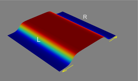
Figure 1: A pair of domain/anti-phase domain wall branes, created near each other at the GUT time scale, separated from one another as the cosmological evolution progressed.

The initial state of the Universe was at a very high temperature and, thus, it was not in the broken phase of the scalar field. Simulations[16, 17] of the $O(N)$ non-linear $\sigma$-model have revealed the phenomena described below. Let us assume that our simulation starts with the system at a high temperature, well above that corresponding to the broken phase, and subsequently the system is rapidly quenched at a temperature below the transition temperature. The initial disordered state of the system relaxes to its ordered broken state in two stages and there are at least two very different time-scales associated with such a two-stage relaxation process. First, different regions of the systems quickly freeze to ordered configurations, which correspond to the broken phase, but different regions choose different orientations of the order parameter, which is fine because the free-energy is $O(N)$ invariant. Namely, because the short-range interactions are stronger, the system minimizes the contribution to the free-energy from these interactions quickly, without paying much attention to find a common global direction of the order parameter. This type of information would take a longer time-scale to be communicated throughout the various regions of the system. An example is shown in Fig. 6 of Ref.[16] for the $O(3)$ non-linear $\sigma$-model in 2+1 dimensions. Because of the $O(N)$ symmetry, which would be spontaneously broken below the transition temperature, there is a manifold of possible order-parameter orientations all of which share the same magnitude that yields the minimum action. The system attempts to align these domains in the second stage of freezing, however, now this takes a much-much longer time-scale to reach an equilibrium where these defects are mutually annihilated. This state of randomly oriented ordered domains corresponds to a very long-lived matastable state because the time-scale grows exponentially with the domain volume.

This is also well-known in experimental physics when, in the absence of an external field, we cool down an $O(N)$-invariant magnetic system, i.e., with no internal anisotropy which can impose a preferred direction. Cooling such a system from its high-temperature non-magnetic phase down to the magnetically ordered phase, the so-called Curie-Weiss magnetic domains form below the critical temperature.

We expect the formation of these domain to also occur in higher dimensions. In fact, we expect that these domains, which are mean-field solutions, should be more protected against thermal and quantum fluctuations in higher dimensions. In fact, renormalization group calculations based on the $\epsilon=4-d$ expansion[18] show that above the upper critical dimension $d_{c}=4$ the mean-field like picture is expected to hold.

Therefore, one would expect a similar scenario to happen in the initially very hot Universe which undergoes rapid cooling. We would expect several DW-aDW pairs, i.e., twists of the local scalar-field VEV (such as those illustrated in Fig. 1), to appear as the temperature cools below the critical temperature which corresponds to its broken phase. We would assume that our Universe exists as one DW, which appears next to an aDW as schematically illustrated in Fig. 1. In the present work, we have assumed a compact geometry, i.e., periodic boundary conditions (PBC) along the fifth dimension. The total phase of the VEV of the background field, which behaves as an order parameter, changes by $\pi$ when crossing a single domain wall and this gives a non-zero value in a type of topological charge associated with the order-parameter phase. However, the total topological charge when we have a combination of a DW-aDW pair is zero and thus, this can occur as a non-equilibrium spontaneous vacuum fluctuation of the background field at an early epoch of the cosmological evolution when the Universe was hot and rapidly cools below a characteristic temperature and enters the ordered phase (like two Weiss domains). On the other hand, just a single DW can not emerge spontaneously in the case where the extra dimensions are compactified. In this case, DWs can only occur in DW-aDW pairs, where the VEV to right of the right DW (blue domain of Fig. 1) and to the left of the left aDW (also blue domain of Fig. 1) are the same and the can match when PBC (compact) are applied. We will assume that the two domain walls were naturally close at the time of their emergence and the distance $d$ between them increases during the cosmological expansion in the same way as the 3+1 DW expands. Namely, it is natural to assume that the “fabric” of of the 3+1D DW expands, as observed, because the 4+1 D bulk expands as a whole.

This leads to the following Dirac equation in 4+1 dimensions:

$$(i\gamma^{\mu}\partial_{\mu}+\gamma^{5}\partial_{4}-h\eta)\Psi=0,$$ (6)

where $x_{\mu}$, $\mu=0,1,2,3$ are the four components of the 3+1 spacetime coordinates and $x_{4}$ is the extra dimension. Let us choose the origin of the extra dimension to be in the middle between the DW and the aDW so that the locations of the left DW $x_{L}$ and of the right aDW $x_{R}$ respectively are related as $x_{L}=-x_{R}$ and $x_{R}>0$. We will express the background scalar field $\eta$ which couples to the fermions as

$$\eta(x_{4}<0) = v\tanh(\kappa(x_{4}-x_{L})),$$

$$\eta(x_{4}>0) = -v\tanh(\kappa(x_{4}-x_{R})),$$ (7)

The above Eq. 7 is a combination of an anti-phase domain walls separated by a distance $d=|x_{R}-x_{L}|$. When $d\to\infty$ the two domain walls are each a saddle point solution to the scalar field action. Our function $\eta$ is schematically illustrated in Fig. 1 for the 2+1 dimensional case where visualization is possible. In the present work, when we discuss the cosmological evolution, the Universe, as a whole at early epochs, is considered bound as it expands. Therefore, Fig. 1 should be considered as a drawing of a portion of the DW-aDW, i.e., from a local viewpoint, and it should not imply that the 4D bulk is infinitely extended.

We can imagine a scenario where these two domain walls were created very close at the early stages of the cosmological evolution (because out of nothing only pairs of domain walls of opposite topological charge can be created) and they are separated from each other at a later time. We want to use a framework to understand this evolution, so it is convenient to use as basis the state of the well-separated domain walls. The reason for considering a pair of such anti-phase domain walls is that each domain wall is characterized by a non-zero topological charge associated with the background field configuration. The pair has zero topological charge and their creation is easier to imagine, whereas creating just an isolated domain wall requires changing the resting configuration from $-\infty$ all the way to $+\infty$. The pair of opposite topological charges belongs to the same topological sector as the flat configuration, whereas the single domain wall configuration is separated from the no-domain wall configuration by an infinite action barrier.

We will assume that the two domain walls were naturally close to each other at the time of their creation and they separated as the time went on because of the expansion in the same way as the 3+1 DW expands. We would like to analyze the early stage of the domain/anti-domain wall system in terms of the easier to conceptualize asymptotic states of two infinitely separated domain-walls. This approach is similar to that in solid state or in molecular physics where the state of many atoms is analyzed in terms of hopping of electrons between atomic orbitals, the so-called tight-binding approximation[19]. In the case where the DW is far away from aDW, we write the solution of the Dirac Eq. 6 as

$$\Psi(x_{\mu},x_{4})=\psi(x_{\mu})f(x_{4}),$$ (8)

where the spinor $\psi(x_{\mu})$ describes a 3+1 dimensional massless fermion, $i\gamma^{\mu}\partial_{\mu}\psi=0$, which is localized on either of the domain walls, and the function $f(x_{4})$ specifies where the fermion is localized along the extra dimension $x_{4}$ and it is obtained as a solution to the following differential equation:

$$(f^{\prime}\gamma^{5}-h\eta f)\psi=0.$$ (9)

We can choose our basis for the spinor part $\psi$ to be the eigenstates of the chirality operator $\gamma^{5}$, for massless fermions, i.e., $\gamma^{5}\psi^{+}=\psi^{+}$, and $\gamma^{5}\psi^{-}=-\psi^{-}$, and in this case the above equation splits into the following two:

$$f^{-\prime}+h\eta f^{-} = 0,$$ (10)

$$f^{+\prime}-h\eta f^{+} = 0,$$ (11)

and the general solution to Eq. 9 may be approximately written as follows:

$$\Psi=f^{-}(x_{4})\psi^{-}(x_{\mu})+f^{+}(x_{4})\psi^{+}(x_{\mu}),$$ (12)

where $f^{-}$ and $f^{+}$ are the most general solutions to the Eqs. 10,11. This approximation makes sense when the two DWs are well-separated, i.e., when $\kappa|x_{R}-x_{L}|>>1$.

We divide the extra dimension in two regions , the region of $x_{4}$ near the left domain wall, i.e., region $L$ ($x_{4}<0$) and the case where $x_{4}>0$ (region $R$). We can integrate Eqs. 10,11 and find that in region $L$ ($x_{4}<0$)

$$f_{L}^{-}(x_{4}<0) = {c^{-}_{L}}\xi(x_{4}-x_{L}),$$ (13)

$$f_{L}^{+}(x_{4}<0) = {{c^{+}_{L}}\over{\xi(x_{4}-x_{L})}},$$ (14)

$$\xi(x) \equiv [\cosh(\kappa x)]^{-hv/\kappa}.$$ (15)

However, because of the wavefunction normalizability condition, we need to choose $c^{+}_{L}=0$. Similarly for region $R$, the solutions are of the form

$$f_{R}^{-}(x_{4}>0) = {{c^{-}_{R}}\over{\xi(x_{4}-x_{R})}},$$ (16)

$$f_{R}^{+}(x_{4}>0) = {c^{+}_{R}}{\xi(x_{4}-x_{R})}.$$ (17)

The normalizability condition in this case yields $c^{-}_{R}=0$. Therefore, there are only left-handed acceptable solutions in the left domain wall, i.e.,

$${U}^{-}_{L} = {C^{-}_{L}}\xi(x_{4}-x_{L})e^{-i(E_{+}x_{0}-{\bf p}\cdot{\bf x})}u^{-}_{L},$$ (18)

$${V}^{-}_{L} = {D^{-}_{L}}\xi(x_{4}-x_{L})e^{-i(E_{-}x_{0}-{\bf p}\cdot{\bf x})}v^{-}_{L},$$ (19)

and right-handed acceptable solutions in the right domain wall,

$$U^{+}_{R} = {C^{+}_{L}}\xi(x_{4}-x_{R})e^{-i(E_{+}x_{0}-{\bf p}\cdot{\bf x})}u^{+}_{R},$$ (20)

$$V^{+}_{R} = {D^{+}_{L}}{\xi(x_{4}-x_{R})}e^{-i(E_{-}x_{0}-{\bf p}\cdot{\bf x})}v^{+}_{R},$$ (21)

where $u^{s}_{L}$ ($u^{s}_{R}$) are chirality-$s$ positive-energy solutions localized on the left (right) DW and $v^{s}_{L}$ ($v^{s}_{R}$) are chirality-$s$ negative-energy solutions localized on the left (right) DW. The constants $C^{\pm}_{L,R}$ and $D^{\pm}_{L,R}$ are coefficients to be determined by the wavefunction normalization condition. When the two DWs are close to each other, the wavefunctions localized on the left and right DWs begin to overlap. In this case, these wavefunctions, which are localized at the centers $x_{R}$ and $x_{L}$, can be used as an unperturbed basis to define an effective $4\times 4$ Hamiltonian where the other degrees of freedom from the extra dimension are implicitly integrated out. First, the zero point motion of the scalar field around this fixed field configuration has been integrated out. Namely, small amplitude fluctuations of this type can be also included, by carrying out path integration of Gaussian fluctuations around the extrema (the DW-aDW solutions). These will only change the matrix elements $V$ and $U$ by a prefactor. However, our qualitative analysis does not rely on specific values of these amplitudes.

The role of higher-energy fermion excitations seem to have also been excluded from the calculation. However, one can imagine that this calculation is based on a quasi-degenerate perturbation theory calculation[20, 19] where our model subspace is defined by a projection operator $\hat{M}=|1\rangle\langle 1|+|2\rangle\langle 2|+|3\rangle\langle 4|+|4\rangle\langle 4|$, which is formed by these four states, and all the other states form a space $\hat{Q}=\sum_{n\neq 1,2,3,4}|n\rangle\langle n|$. Then, the effective Hamiltonian, which operates only in the reduced subspace spanned by these 4 states is obtained by including the virtual excitations to states outside this subspace perturbatively. The inclusion of these states only modifies the values of amplitudes $V$ and $U$. In the present paper, we assumed that by integrating out these virtual excitations we remain in this reduced 4-dimensional subspace. Again, our qualitative analysis does not depend on the specific values of the matrix elements $V$ and $U$ used above.

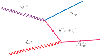
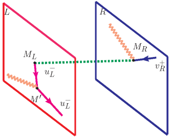
Figure 2: (a) The well-known pair production process. (b) The pair production where the antiparticle is created by a photon on the right DW and at the same time a particle is created on the left DW. The rest of the process on the left DW is similar to that in (a).

3 Generation of the baryon asymmetry

Localizing the gauge field on the DW branes giving the correct SM on the brane might be tricky[21]. Here, because of the requirement of gauge invariance we will consider the minimal coupling of a gauge field to the fermions, i.e.,

$$\hat{H}_{int} = {\bf J}\cdot{\bf A},$$ (22)

$${\bf J} = e\Psi^{\dagger}\hat{\vec{\alpha}}\Psi,$$ (23)

and we are working in a gauge where $A_{0}=0$, and $\hat{\alpha}_{i}$, $i=1,2,3$ are the three Dirac matrices, and

$$\hat{\alpha}_{4} = -i\gamma^{0}\gamma^{5}=-i\left(\begin{array}[]{cc}~{}~{}{\bf 0}&\hat{\bf 1}\\ -\hat{\bf 1}&{\bf 0}\end{array}\right).$$ (26)

This form of the current is consequence of Noether’s theorem. At the early epoch after the Big-Bang the high-energy photons are believed to create particle/antiparticle pairs. Let us consider the process which generates electron-positron pairs as an example. The first order process of a single photon creating an electron-positron pair cannot simultaneously conserve energy and momentum. The leading process is a second-order process where two photons produce an electron-positron pair. Following Dirac[22] we consider this process in 4+1 dimensions in the presence of the DW-aDW pair discussed previously. We consider the field produced by two photons localized on one domain-wall and propagating on the 3+1 brane $x_{\mu}$. However, their polarization vectors ${\bf a}_{1,2}$, which are perpendicular to their momenta ${\bf q}_{1,2}$ due to gauge invariance, can be perpendicular to the domain-wall, i.e., along the dimension $x_{4}$. The vector potential can be written as

$$A_{\mu} = \Bigl{[}{\bf a}_{\mu L}^{\dagger}e^{-i(q_{L}x_{0}-{\bf q}_{L}\cdot{\bf x})}+{\bf a}_{\mu L}e^{i(q_{L}x_{0}-{\bf q}_{L}\cdot{\bf x})}\Bigr{]}\zeta_{\mu L}$$ (27)

$$+ \Bigl{[}{\bf a}_{\mu R}^{\dagger}e^{-i(q_{R}x_{0}-{\bf q}_{R}\cdot{\bf x})}+{\bf a}_{\mu R}e^{i(q_{R}x_{0}-{\bf q}_{R}\cdot{\bf x})}\Bigr{]}\zeta_{\mu R},$$

where ${\bf a}_{L}$ (${\bf a}_{R}$) is along the polarization vector $\epsilon_{\mu}$ of the photon localized on the $L$ ($R$) domain-wall. There are three possible directions of polarization, and they are all perpendicular to the direction of momentum, which is assumed to lie on the 3+1 brane. We will consider the role of the gauge field localized on the DWs, but on one of the DWs, say the ${\bf a}_{R}$, having polarization along the extra dimension, i.e., that ${\bf a}_{R}$ is along $x_{4}$, while on the other DW, ${\bf a}_{L}$ can be with polarization vector with components in the DW. The function $\zeta_{L,R}=g(x_{4}-x_{L,R})$ is the profile of a gauge-field localization function along the dimension $x_{4}$. There are several matrix-elements of $\hat{H}_{int}$ between the states listed in Eqs. 18,19,20,21. Owing to the fact that

$$\hat{\alpha}_{4}u^{+}=-iv^{-},\hskip 14.45377pt\hat{\alpha}_{4}u^{-}=iv^{+},$$ (28)

$$\hat{\alpha}_{4}v^{+}=-iu^{-},\hskip 14.45377pt\hat{\alpha}_{4}v^{-}=iu^{+},$$ (29)

tracing over the degrees of freedom of the $x_{4}$ direction, the following matrix elements of the 4th component of the current operator are non-zero:

$$\langle V^{-}_{L}|J_{4}|U^{+}_{R}\rangle,\hskip 14.45377pt\langle V^{+}_{R}|J_{4}|U^{-}_{L}\rangle,$$ (30)

$$\langle U^{-}_{L}|J_{4}|V^{+}_{R}\rangle,\hskip 14.45377pt\langle U^{+}_{R}|J_{4}|V^{-}_{L}\rangle,$$ (31)

which are proportional to the overlap integral $I_{f}$ of the wavefunction profiles along the $x_{4}$ direction of the fermion parts:

$$I_{f}=C^{\pm}_{R}[C^{{\mp}}_{L}]^{*} \int {dx_{4}}\xi(x_{4}-x_{L})\xi(x_{4}-x_{R}).$$ (32)

Assuming that the DWs are close enough such that this integral has a significant value, the matrix elements above are non-zero. In order to have a non-zero vertex for processes such as the one illustrated in Fig. 2, i.e., for example, to create an electron on the right DW and a positron on the left DW due to an incident photon on the left DW, we need to consider the matrix element of the gauge field operator that contains the term

$$\langle 0|a^{\dagger}_{4,L}a^{\dagger}_{4,R}|0\rangle.$$ (33)

This matrix element is proportional to the following overlap integral

$$I_{b}=\int dx_{4}\zeta(x_{4}-x_{L})\zeta(x_{4}-x_{R}).$$ (34)

In order for the vertex to split over the two DWs (shown as $M_{L}$ and $M_{R}$ in Fig. 2), the DW needs to be at a distance from the aDW less than the spread of the localization function of fermions $\xi(x)$ and of the gauge fields $\zeta(x)$. The rest of the process shown in Fig. 2 which takes place on the left DW in our example, is the same as in Fig. 2. This part requires the polarization of the ${\bf a}^{\dagger}_{R}$ to be in the left DW brane dimensions. Notice that the momentum, energy, charge and parity conservation is fulfilled if we consider all the inter-DW parts together. They are not conserved on each DW individually.

4 Discussion of critical issues

As mentioned in the Introduction, there are several domain-wall models that have been proposed by various investigators in order to explain the emergence of the 3+1 dimensional space out of a higher dimensional space. The goal of the present paper was to build on the domain-wall models aiming to obtain one that is more consistent with statistical physics and thermodynamics and to explain the matter-antimatter asymmetry. Embedding this braneworld scenario in a consistent UV theory and providing a full explanation of the cosmological evolution are challenging issues and are beyond the scope of the present paper. Such questions are not unique to our model, they are issues for all the domain-wall braneworld models and they are currently being addressed by various investigations. Below we list some of these critical issues of these models and of our present proposal.

There are various different philosophies on how to localize the gauge field on the DW brane. Dvali and Shifman[21] relies on the non-perturbative nature of confinement: they consider strongly-coupled gauged theories which can be in the non-Abelian confining phase outside the DW and in the Abelian Coulomb phase inside the DW. This picture is complementary to the dual superconductor model of confinement first proposed by t’Hooft and Mandelstam where confinement arises due to a magnetic monopole condensate[23]. In other attempts[14, 24] a gauge coupling that depends on the extra dimensions is used where, when trying to separate the extra component of the gauge field from the other four components $A_{\mu}$, it is found that the relation between the $A_{\mu}$ and its fifth component in the 4-dimensional effective theory is the one between a massive gauge boson and a would-be Goldstone mode after the spontaneous gauge symmetry breaking. In this case, the KK-modes of the fifth component are identified as the Goldstone modes which would be eaten by the KK-modes of $A_{\mu}$. This can happen if the parameters are chosen properly and after the symmetry breaking, which happened at the GUT scale.

On the other hand, the scenario, which we describe in the present work, is for the epoch before the GUT scale. Another scenario might be that the fluctuations which we describe in this work correspond to other KK modes and not to the zero mode.

Critical issues are the details of the expansion of this 4+1 dimensional braneworld and how the evolution of the DW-aDW system couples to the inflation and the rest of the cosmic evolution. This connection is very important, precisely because inflation dictates that baryon asymmetry must be dynamically generated after reheating, necessitating a mechanism of baryogenesis. We have generalized the expansion of our Universe to an expanding 4+1 dimensional spacetime where the 3+1D DW (our Universe) and aDW necessarily expand. One important difference from other braneworld models is that in the present scenario we need to consider the role of the characteristic time-scale when, because of this expansion, the DW-aDW separation $d$ becomes of the order of or greater than the DW thickness, i.e., 1/$\kappa$. The Planck data[25] from the cosmic microwave radiation and the current information on the elemental density in the Universe should be analyzed to determine how this time-scale is related to the hierarchy of the various other time-scales of the cosmological evolution, such as, the inflation epoch as well as the inflaton density evolution. Furthermore, new information from the detection of gravitational waves imposes further constraints on the present and other braneworld models[26, 27, 28]. Therefore, an investigation of the relationship of the scenario presented in this paper where more special-case scenarios are discussed and the inflation is urgently needed.

5 Conclusions

The mechanism described here allows for a matter-antimatter asymmetry to appear separately in the DW and the aDW, without allowing such asymmetry to occur in the combined DW-aDW system. Therefore, when the Universe was in a very high temperature state, where the occurrence of pair creation events should be considered statistically independent, a matter-antimatter asymmetry is allowed to happen in each of the two DW subsystems. Given that more than one type of SM particle-antiparticle creation processes take place, the overall charge neutrality on each DW can be maintained not necessarily by means of having equal number of particles and anti-particles of each type. In addition, momentum, energy, charge and parity conservation are all fulfilled if we consider the DW-aDW system together.

The mechanism does not rely on the particular means of the gauge field localization. It is only using the fermion field localization on a DW-aDW pair. We see no reason that by localizing the gauge field on a DW brane would mean that the gauge field cannot have polarization along the extra dimension in the early epoch of the cosmological evolution. However, as discussed earlier, this problem of localizing the gauge field on the DW is tricky.

Photons with polarization along the extra dimension, in order to be absorbed by a fermion bound to the DW brane, require a change in the chirality of the particle. The only first order process of this type is the one discussed in this work involving a photon with such polarization, but it was only applicable when the Universe was of microscopic size, i.e., when the matter localization length on the DW was comparable to the DW-aDW separation. This process is exponentially suppressed as a function of the DW-aDW distance and, thus, in a Universe where the DW and the aDW are well-separated, it is exponentially unlikely. As a result, when the DW and the aDW are well-separated, these photons are not allowed to interact with standard model particles except that they might contribute to the total energy density that causes curvature. There are various scenarios to include their role in the cosmological evolution in order to explain the high-resolution Planck data[25]. These, along with addressing the critical issues listed in the previous Section, require a detailed future study.

6 Acknowledgments

The author would like to thank W. H. Green for an enlightening discussion about the analysis of the high resolution Planck data of the cosmic microwave background radiation.

References

- Kaluza [1921] T. Kaluza, Zum Unitätsproblem der Physik, Sitzungsberichte der Königlich Preußischen Akademie der Wissenschaften (Berlin (1921) 966–972.
- Klein [1926] O. Klein, The Atomicity of Electricity as a Quantum Theory Law, Nature 118 (1926) 516.
- Green and Schwarz [1984] M. B. Green, J. H. Schwarz, Anomaly cancellations in supersymmetric d = 10 gauge theory and superstring theory, Physics Letters B 149 (1984) 117–122.
- Dai et al. [1989] J. Dai, R. Leigh, J. Polchinski, New connections between string theories, Modern Physics Letters A 04 (1989) 2073–2083.
- Polchinski [1995] J. Polchinski, Dirichlet branes and ramond-ramond charges, Phys. Rev. Lett. 75 (1995) 4724–4727.
- Green et al. [2012] M. B. Green, J. H. Schwartz, E. Witten, Superstring Theory 25th Anniversary Edition: Volume 1: Introduction, Cambridge Monographs on Mathematical Physics, Cambridge, 2012.
- Witten [1996] E. Witten, Strong coupling expansion of calabi-yau compactification, Nuclear Physics B 471 (1996) 135 – 158.
- Horava and Witten [1996a] P. Horava, E. Witten, Heterotic and type i string dynamics from eleven dimensions, Nuclear Physics B 460 (1996a) 506 – 524.
- Horava and Witten [1996b] P. Horava, E. Witten, Eleven-dimensional supergravity on a manifold with boundary, Nuclear Physics B 475 (1996b) 94 – 114.
- Arkani-Hamed et al. [1998] N. Arkani-Hamed, S. Dimopoulos, G. Dvali, The hierarchy problem and new dimensions at a millimeter, Physics Letters B 429 (1998) 263 – 272.
- Randall and Sundrum [1999] L. Randall, R. Sundrum, Large mass hierarchy from a small extra dimension, Phys. Rev. Lett. 83 (1999) 3370–3373.
- Jackiw and Rebbi [1976] R. Jackiw, C. Rebbi, Solitons with fermion number ½, Phys. Rev. D 13 (1976) 3398–3409.
- Davies et al. [2008] R. Davies, D. P. George, R. R. Volkas, Standard model on a domain-wall brane?, Phys. Rev. D 77 (2008) 124038.
- Okada et al. [2019] N. Okada, D. Raut, D. Villalba, Domain-wall standard model in non-compact 5d and lhc phenomenology, Modern Physics Letters A 34 (2019) 1950080.
- George and Volkas [2007] D. P. George, R. R. Volkas, Kink modes and effective four dimensional fermion and higgs brane models, Phys. Rev. D 75 (2007) 105007.
- Bitar and Manousakis [1991] K. Bitar, E. Manousakis, Nonlinear model and static holes, Phys. Rev. B 43 (1991) 2615–2624.
- Manousakis and Salvador [1989] E. Manousakis, R. Salvador, Equivalence between the nonlinear model and the spin-1/2 antiferromagnetic heisenberg model: Spin correlations in , Phys. Rev. B 40 (1989) 2205–2216.
- Wilson and Kogut [1974] K. G. Wilson, J. Kogut, The renormalization group and the expansion, Physics Reports 12 (1974) 75–199.
- Manousakis [2016] E. Manousakis, Practical Quantum Mechanics: Modern Tools and Applications, Oxford University Press, New York, 2016.
- Lepetit and Manousakis [1993] M.-B. Lepetit, E. Manousakis, Real-space renormalization-group studies of low-dimensional quantum antiferromagnets, Phys. Rev. B 48 (1993) 1028–1035.
- Dvali and Shifman [1997] G. Dvali, M. Shifman, Domain walls in strongly coupled theories, Physics Letters B 396 (1997) 64 – 69.
- Dirac [1930] P. A. M. Dirac, On the annihilation of electrons and protons, Mathematical Proceedings of the Cambridge Philosophical Society 26 (1930) 361–375.
- Peskin [1978] M. E. Peskin, Mandelstam-t’hooft duality in abelian lattice models, Annals of Physics 113 (1978) 122–152.
- Ohta and Sakai [2010] K. Ohta, N. Sakai, Non-Abelian Gauge Field Localized on Walls with Four-Dimensional World Volume, Progress of Theoretical Physics 124 (2010) 71–93.
- Aghanim et al. [2020] N. Aghanim et al., Planck 2018 results - vi. cosmological parameters, A&A 641 (2020) A6.
- Du et al. [2021] Y. Du, S. Tahura, D. Vaman, K. Yagi, Probing compactified extra dimensions with gravitational waves, Phys. Rev. D 103 (2021) 044031.
- Mohammadi et al. [2020] A. Mohammadi, T. Golanbari, S. Nasri, K. Saaidi, Constant-roll brane inflation, Phys. Rev. D 101 (2020) 123537.
- Visinelli et al. [2018] L. Visinelli, N. Bolis, S. Vagnozzi, Brane-world extra dimensions in light of gw170817, Phys. Rev. D 97 (2018) 064039.