Impact of calibration uncertainties on Hubble constant measurements from gravitational-wave sources

Abstract

Gravitational-wave (GW) detections of electromagnetically bright compact binary coalescences can provide an independent measurement of the Hubble constant $H_{0}$. In order to obtain a measurement that could help arbitrating the existing tension on $H_{0}$, one needs to fully understand any source of systematic biases for this approach. In this study, we aim at understanding the impact of instrumental calibration errors (CEs) and uncertainties on luminosity distance measurements, $D_{L}$, and the inferred $H_{0}$ results.We simulate binary neutron star mergers (BNSs), as detected by a network of Advanced LIGO and Advanced Virgo interferometers at their design sensitivity. We artificially add CEs equal to exceptionally large values experienced in LIGO-Virgo’s third observing run (O3). We find that for individual BNSs at a network signal-to-noise ratio of 50, the systematic errors on $D_{L}$– and hence $H_{0}$– are still smaller than the statistical uncertainties. The biases become more significant when we combine multiple events to obtain a joint posterior on $H_{0}$. In the rather unrealistic case that the data around each detection is affected by the same CEs corresponding to the worst offender of O3, the true $H_{0}$ value would be excluded from the 90% credible interval after $\sim 40$ sources. If instead 10% of the sources suffer from severe CEs, the true value of $H_{0}$ is included in the 90% credible interval even after we combine 100 sources.

I Introduction

The Hubble constant, $H_{0}$, is the current expansion rate of the Universe and serves an important role in our understanding of the cosmic expansion history. However, currently there exists a 4.4-$\sigma$ tension between the measurements of early and late Universe. Planck satellite’s observations of the cosmic microwave background anisotropies, assuming the standard flat cosmological model, lead to an inferred late-Universe measurement of $H_{0}=67.36\pm 0.54~{}\mathrm{km\ s}^{-1}\mathrm{Mpc}^{-1}$ Abbott et al. (2018a); Aghanim et al. (2020). Direct measurements in the local universe lead to a different result: the SH0ES team measured $H_{0}=74.03\pm 1.42~{}\mathrm{km\ s}^{-1}\mathrm{Mpc}^{-1}$ using the Cepheid-supernova distance ladder Riess et al. (2016, 2018), consistent with results from H0LiCOW using lensed quasars Birrer et al. (2019); Wong et al. (2020), or from the Carnegie-Chicago Hubble program using the Tip of the Red Giant Branch method to calibrate the distances Jang and Lee (2017); Freedman et al. (2019); Kim et al. (2020).

Compact binary coalescences that are both electromagnetically (EM) bright and emit substantial gravitational waves (GWs) provide an independent method to measure $H_{0}$, and have the potential to resolve this tension Schutz (1986); Holz and Hughes (2005); Dalal et al. (2006); Nissanke et al. (2010, 2013); Chen et al. (2018); Hotokezaka et al. (2019); Soares-Santos et al. (2019); Feeney et al. (2021). Multi-messenger observations of a compact binary coalescence yield a measurement of the luminosity distance $D_{L}$ from the GW observations, and a measurement of the Hubble flow velocity $v_{H}$ from the EM observations. Combining these measurements leads to a direct estimation of $H_{0}$, a method often referred to as “bright sirens” measurement. Since EM-bright GW sources detected by the second-generation GW detectors will be relatively local, we can only use bright sirens to constrain $H_{0}$. Other cosmological parameters can be measured with methods that rely on neutron star (NS) equation-of-state Messenger and Read (2012); Del Pozzo et al. (2017); Dietrich et al. (2020), dark sirens Schutz (1986); Del Pozzo (2012); Abbott et al. (2021, 2021); Soares-Santos et al. (2019); Gray et al. (2020), features in the mass distribution of binary neutron star mergers (BNSs) and binary black hole mergers (BBHs) Taylor et al. (2012); Farr et al. (2019); Mastrogiovanni et al. (2021); Finke et al. (2021), or the spatial clustering scale of GW sources with known galaxies Mukherjee et al. (2021a); Diaz and Mukherjee (2021).

The observations of GW170817 by the LIGO and Virgo network Abbott et al. (2018b); Barsotti et al. (2018); Collaboration (2015); Tse et al. (2019), together with the kilonova AT2017gfo and the gamma-ray burst GRB170817A, served as the first demonstration of the bright siren approach, leading to a measurement of $H_{0}=70.0^{+12.0}_{-8.0}~{}\mathrm{km\ s}^{-1}\mathrm{Mpc}^{-1}$  Abbott et al. (2017a, b, c, d, 2019). This method can be very powerful in the future, as we observe more such events. Ref. Nissanke et al. (2013) presented a 5% precision in the $H_{0}$ measurement after 15 BNSs with EM counterparts, and 1% with 30 sources. However, GW observations may suffer from underlying systematic biases in their estimate of $D_{L}$, and one needs to understand these biases before interpreting the resulting $H_{0}$ measurements. One such bias is the systematic error in the production and calibration of the detectors’ primary data stream Hall et al. (2019); Sun et al. (2020, 2021), referred to as calibration errors (CEs). Such errors are uncorrelated with the astrophysical event rate, evolve independently in each detector, and may be present in one or more detectors during several astrophysical events. CEs may bias the amplitude of the strain data in the same way over multiple observations, and lead to a biased inference of $H_{0}$.

Previous studies have estimated the impact of typical values of CEs seen in the LIGO-Virgo’s first and second observing runs on individual events alone Vitale et al. (2012); Payne et al. (2020); Vitale et al. (2021), or attempted to refine the estimates of CEs using detected Essick and Holz (2019) or expected astrophysical signals Schutz and Sathyaprakash (2020). Our study instead uses large systematic errors as experienced during atypical times in the LIGO-Virgo’s third observing run (O3) to probe their worst-case impact on astrophysical parameter estimation (PE) for both the single-event characterization and the joint inference of $H_{0}$.

More specifically, we simulate a collection of BNS detections, and introduce into the GW data stream artificial CEs that follow six cases of particularly large CEs from the Advanced LIGO detectors at Hanford (LHO) or Livingston (LLO) during O3 Sun et al. (2020, 2021). We pick the instantiation that leads to the worst bias in the astrophysical measurements of $D_{L}$, apply it to varying fractions of 100 simulated BNSs and infer $H_{0}$ to explore the progressive impact of large CEs. In Sec. II, we will discuss the method we use to produce the miscalibrated data stream and to perform PE. In Sec. III, we report how CEs impact the $D_{L}$ results for individual events, as well as the $H_{0}$ results when we combine multiple sources.

II Method

In Sec. II.1, we summarize how we simulate the data stream; in Sec. II.2 how we define CEs and artificially add them to the data stream; and in Sec. II.3 how we perform PE and infer $H_{0}$.

II.1 Simulations

We simulate 5,000 BNSs with uniform-in-cosine inclinations and sky localizations uniformly distributed on the sky. Each event is assigned a $D_{L}$ randomly drawn from a uniform-in-comoving-volume distribution. The maximum $D_{L}$ is set at 600 Mpc, larger than the horizon of a LIGO-Virgo network at the design sensitivity Abbott et al. (2018b); Barsotti et al. (2018). We randomly draw 100 events with network SNRs above 12 to form our set of EM-bright GW events.

We simulate non-spinning BNSs with component masses $m_{1}=2M_{\odot}$ and $m_{2}=1.5M_{\odot}$, using the phenomenological waveform model IMRPhenomPv2 Husa et al. (2016); Khan et al. (2016); Hannam et al. (2014); Smith et al. (2016). We use the same waveform model during PE in order to avoid any systematics caused by waveform mismatch. For all of the BNSs in our study, we do not include any NS tidal deformability in our analysis, as IMRPhenomPv2 does not model neutron star matter effects. We assume that an EM counterpart has been found and yielded an exact redshift measurement. Since the uncertainties on sky localization from the EM side are much smaller than the typical uncertainties on the GW side, we assume the sky position of the sources to be exactly known from the EM observations prior to the GW analysis. We also disregard effects from the peculiar velocity of the sources, as most of the events considered here are close to the horizon of GW detections.

We produce Gaussian noise ${\bf n}$ colored by the Advanced LIGO and Advanced Virgo design sensitivities Barsotti et al. (2018). We then project the signal, which is the sum of the modeled waveforms and the noise, to each detector of the LIGO-Virgo network to obtain the data stream.

II.2 Systematic Calibration Errors

Each of the current Advanced LIGO and Advanced Virgo detectors is a dual-recycled Fabry-Pérot Michelson laser interferometer (IFO) Buikema et al. (2020); Acernese et al. (2014), and its data stream $\boldsymbol{d}_{\mathrm{IFO}}$ is obtained from a voltage signal, $\boldsymbol{e}_{\mathrm{IFO}}$, measured from the output laser power incident on a photo detector, where the subscript “IFO” indexes the detector. The process of creating a model to convert $\boldsymbol{e}_{\mathrm{IFO}}$ into $\boldsymbol{d}_{\mathrm{IFO}}$ is referred to as calibration Viets et al. (2018). For each detector at any given time, the conversion from $\boldsymbol{e}_{\mathrm{IFO}}$ to $\boldsymbol{d}_{\mathrm{IFO}}$ is made by a complex-valued, frequency-dependent response function, $R(f;t)$,

$$\boldsymbol{d}_{\mathrm{IFO}}=R_{\mathrm{IFO}}(f;t)~{}\boldsymbol{e}_{\mathrm{IFO}}.$$ (1)

The model for the response function, $R_{\mathrm{model,IFO}}(f;t)$, is constructed based on the expected behavior of the detectors, coupled with many supporting measurements of the parameters and components of the model as described in Ref. Abbott et al. (2017e); Tuyenbayev et al. (2017). Imperfections in $R_{\mathrm{model,IFO}}(f;t)$, and thus in $\boldsymbol{d}_{\mathrm{IFO}}$, are referred to as calibration errors, or CEs Hall et al. (2019); Sun et al. (2020, 2021). The errors may be represented by the ratio of the true response function, $R_{\mathrm{true,IFO}}(f;t)$, and the model, $R_{\mathrm{model,IFO}}(f;t)$, by

$$\eta_{\rm IFO}(f;t)=R_{\mathrm{true,IFO}}(f;t)/R_{\mathrm{model,IFO}}(f;t).$$ (2)

In the ideal case, $R_{\mathrm{model,IFO}}(f;t)$ will be identical to $R_{\mathrm{true,IFO}}(f;t)$, and $\eta_{\rm IFO}(f;t)$ becomes a frequency-independent constant with unity magnitude and zero phase. In reality, $\eta_{\rm IFO}(f;t)$ is usually a function of frequency and time. Since $R_{\mathrm{model,IFO}}(f;t)$, $R_{\mathrm{true,IFO}}(f;t)$ and $\eta_{\rm IFO}(f;t)$ always depend on $f$ and $t$ in our case and evolve independently in every detector, we will drop the $(f;t)$ arguments and the IFO subscript henceforth unless we need to specify $f$, $t$, or the instrument.

While $R_{\mathrm{model}}$ is known, $R_{\mathrm{true}}$ may only be inferred by direct measurements that are invasive for observations and would reduce the duty cycle of the detector. Instead, $\eta$ is numerically estimated by creating a probability distribution informed by those direct measurements. At a given reference time, $T_{0}$, the parameters of $R_{\mathrm{model}}$ are measured to create $10^{4}$ samples of the probability distribution of $\{\eta(T_{0})\}$, with relatively large uncertainty. Later, additional measurements and models are crafted to better inform or correct the estimated $\{\eta(T_{0})\}$, in retrospect. In O3, the probability distribution of $\eta$ for each detector was estimated regularly at discrete times $\{T\}$ with hourly cadence for times while the detector was stable in the observing mode.

The estimated $\{\eta\}$ may vary slowly in time, either continuously with drifts in the detector’s alignment or thermal state, or discretely with changes made in the detector’s control system between different configuration periods. In most cases, the slow time-dependent variation is appropriately tracked and accounted for when producing $\boldsymbol{e}_{\mathrm{IFO}}$, and thus the time variation of $\{\eta\}$ is negligible for the majority of the observing time as long as the detector’s sensing and control configuration remain unchanged. Over such a particular observing period within static configuration, we can choose an arbitrary moment in time $T_{k}$ such that $\{\eta(T_{k})\}$ represents the typical CE distribution in that period, and refer to this distribution as $\{\eta^{\mathrm{typ}}(T_{k})\}$.

However, the detectors’ sensing and control configurations do not remain static for the entire observing run. There may be planned changes (typically to improve the detector sensitivity) or unplanned changes (due to issues with the hardware, electronics, or computers). Such changes may have either unexpected impact on the calibration, or get fixed in a temporary fashion such that the observation may resume (with an acceptable error) but may not be fully investigated and resolved until later. The entire detector’s response, $R_{\mathrm{model}}$, is checked by weekly measurements, and monitored continuously at a few select frequencies, to ensure coverage of any unexpected situations. When issues are found in the detector behavior, additional measurements may also made such that error may be modeled and included in $\{\eta\}$ retroactively at a later time. If at a time $t_{i}$, $\{\eta(t_{i})\}$ is modeled to be significantly different from $\{\eta^{\mathrm{typ}}(T_{i})\}$ at a nearby time $T_{i}$, we call these outliers $\{\eta^{\mathrm{out}}(t_{i})\}$, henceforth $\{\eta^{\mathrm{out}}\}_{i}$. During O3, six such outliers have been identified in either LLO or LHO. We refer to the corresponding typical error distribution as $\{\eta^{\mathrm{typ}}\}_{i}$, for conciseness.

For example, in Fig. 1, we compare the median and 1-$\sigma$ boundaries of the magnitude and the phase of $\{\eta^{\mathrm{out}}\}_{6,\mathrm{LLO}}$ against its corresponding $\{\eta^{\mathrm{typ}}\}_{6,\mathrm{LLO}}$. We include plots for the distributions of $\{\eta^{\mathrm{out}}\}_{i}$ and $\{\eta^{\mathrm{typ}}\}_{i}$ for $i=1...5$ in App. A. In reality, if there is an astrophysical signal at a time similar to one of the $t_{i}$, its $\{\eta^{\mathrm{out}}\}_{i}$ may not be readily available at the time of PE analyses, and $\{\eta^{\mathrm{typ}}\}_{i}$ will be used instead. This is the scenario we investigate in this study: when the actual CEs are very different from the CEs known and used at the time of PE.

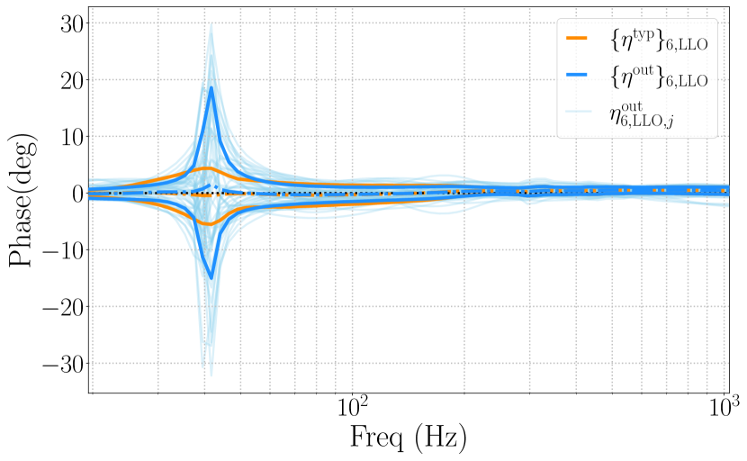
Figure 1: The median (dash-dotted) and the 1-$\sigma$ bounds (solid) of CE distributions from O3 in magnitude (top) and phase (bottom), as a function of frequency. The thick blue curves mark the $1-\sigma$ bound of one example of a large CE, $\{\eta^{\mathrm{out}}\}_{6,\mathrm{LLO}}$, and the thin light blue curves are some of the individual realizations, $\eta^{\mathrm{out}}_{6,\mathrm{LLO},j}$ during this time. The orange curves are the corresponding typical distribution $\{\eta^{\mathrm{typ}}\}_{6,\mathrm{LLO}}$.

We introduce artificial CEs to the data streams $\boldsymbol{d}_{\mathrm{LLO}}$ and $\boldsymbol{d}_{\mathrm{LHO}}$. For all of the six cases, $\{\eta^{\mathrm{out}}\}_{i}$ is only in one of the Advanced LIGO detectors. We will first select the worst realization from each $\{\eta^{\mathrm{out}}\}_{i}$, denoted by $\eta^{\mathrm{mis}}_{i}$, such that it maximizes its impact on the amplitude of the data, and hence on the estimation of the source distance. We define the impact, weighted by the detector sensitivity, and integrated over the bandwidth:

$$\mathcal{D}_{i,j}\equiv\int^{f_{\mathrm{high}}}_{f_{\mathrm{low}}}\frac{|\eta_{i,j}|-\widetilde{|\eta^{\mathrm{typ}}_{i}|}}{\sqrt{S_{n}(f)}}\mathrm{d}f,$$ (3)

where j indexes the curves from each $\{\eta^{\mathrm{out}}\}_{i}$ distribution. At each frequency, we take the difference between $|\eta_{i,j}|$, the magnitude of the $j^{\rm th}$ sample of $\{\eta^{\mathrm{out}}\}_{i}$, and $\widetilde{|\eta^{\mathrm{typ}}_{i}|}$, the median of the magnitudes of samples in $\{\eta^{\mathrm{typ}}\}_{i}$ (the dot-dashed orange curve in Fig. 1). $\sqrt{S_{n}(f)}$ is the amplitude spectral density of the detector’s sensitivity, for which we use aLIGO’s design sensitivity Abbott et al. (2018b); Barsotti et al. (2018). The frequency limits of the integral, $f_{\mathrm{high}}$ and $f_{\mathrm{low}}$, have been chosen as 20 Hz and 1024 Hz, respectively, with a frequency resolution of 0.25 Hz. While the maximum difference may correspond to a positive or negative $\mathcal{D}_{i,j}$ value, we select the curve that maximizes $\mathcal{D}_{i,j}$ in the negative direction, denoted by $\eta^{\mathrm{mis}}_{i}$,

$$\eta^{\mathrm{mis}}_{i}\equiv\underset{j}{\min}\mathcal{D}_{i,j}.$$ (4)

Fig. 2 shows the amplitude and phase of the selected $\eta^{\mathrm{mis}}_{6,\mathrm{LLO}}$ compared against $\{\eta^{\mathrm{typ}}\}_{6,\mathrm{LLO}}$ from Fig. 1. We can use this curve to miscalibrate the LLO data, the sum of the noise and the modeled waveform, as,

$${\boldsymbol{d}}^{\rm mis}_{i}=\eta^{\mathrm{mis}}_{i}~{}\boldsymbol{d}.$$ (5)

The noise, as part of $\boldsymbol{d}$, will thus also be scaled by $\eta^{\mathrm{mis}}_{i}$. The resulted amplitude spectral density of each detector is $\eta^{\mathrm{mis}}_{i}\sqrt{S_{n}(f)}$.

For the other Advanced LIGO detector, in this case LHO, we will apply a sample curve $\eta^{\mathrm{mis}}_{6,\mathrm{LHO}}$ that lies within the 1-$\sigma$ credible interval (CI) from $\{\eta^{\mathrm{typ}}\}_{6,\mathrm{LHO}}$ to the data, in the same way as Eq. (5). No CEs are added to aVirgo data, since the full $\eta$ distributions of aVirgo are not available at the time of writing. In this case, $\{\eta^{\mathrm{mis}}_{6,\mathrm{LLO}},\eta^{\mathrm{mis}}_{6,\mathrm{LHO}},1\}$ forms the set of curves to miscalibrate the data for scenario #6.

We also prepare a separate set of control runs in which we do not add any CE in any of the detectors. When comparing PE results of the miscalibrated runs and the control runs, we thus observe biases exclusively caused by the large added CEs in the former.

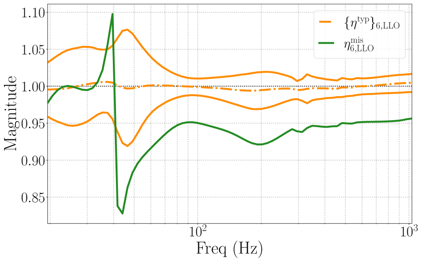
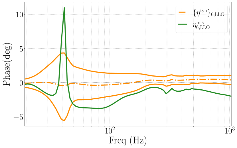
Figure 2: $\eta^{\mathrm{mis}}_{6,\mathrm{LLO}}$ (green) shown in magnitude and phase (deg) as a function of frequency (Hz). Also plotted are the 1-$\sigma$ bounds and the median of typical CE distributions, $\{\eta^{\mathrm{typ}}\}_{6,\mathrm{LLO}}$ (orange).

Next, we select one CE realization that leads to the most significant bias in the $D_{L}$ likelihood, and apply it to 100 segments of data, each containing a different BNS event, as described in Sec. II.1. To select the desired CE realization, we first consider a single BNS event with network SNR of 50, inclination 30^∘, and located right above LLO in the sky. We add each of the six distinctive sets of CEs to a data chunk containing this BNS, and compare the resulting $D_{L}$ likelihoods. As we only consider single-event results in this part of the study, we work with zero noise Vallisneri (2008) to eliminate random effects of noise realizations. We finally We use the zero-noise realization where the noise ${\bf n}$ has mean of ${\bf 0}$ and standard deviation equal to the detector power spectral density. Lastly, we infer $H_{0}$ from the 100 events.

II.3 Parameter Estimation and Inference of $H_{0}$

We perform Bayesian inference Veitch et al. (2015); Abbott et al. (2016) to obtain the likelihood $\mathcal{L}({\boldsymbol{d}}|\boldsymbol{\theta},H_{0},\mathcal{H})$, where $\boldsymbol{\theta}$ is the set of astrophysical parameters, under model $\mathcal{H}$. We write $H_{0}$ explicitly because it is a hyperparameter that we are interested in. We can obtain the likelihood $\mathcal{L}(\boldsymbol{d}|H_{0},\mathcal{H})$ by integrating over all astrophysical parameters,

$$\mathcal{L}(\boldsymbol{d}|H_{0},\mathcal{H})=\int\mathrm{d}\boldsymbol{\theta}\mathcal{L}(\boldsymbol{d}|\boldsymbol{\theta},H_{0},\mathcal{H})\pi(\boldsymbol{\theta}|H_{0},\mathcal{H}),$$ (6)

where $\pi(\boldsymbol{\theta}|H_{0},\mathcal{H})$ is the prior. We use a uniform prior for $\pi(H_{0}|\mathcal{H})=[20,150]\mathrm{km\ s}^{-1}\mathrm{Mpc}^{-1}$ to obtain a posterior distribution $p(H_{0}|{\boldsymbol{d}},\mathcal{H})$ from the likelihood in Eq. (6). Since not all events have equal chances to be detected, we follow Ref.  Chen et al. (2018); Vitale et al. (2020) to account for selection effects, and call the function of detectable sources $\beta(H_{0})$. Since all sources in our simulations have the same source-frame masses, the selection function only needs to be calculated once for all the events. We can finally obtain the posterior for $H_{0}$ as,

$$p(H_{0}|{\boldsymbol{d}},\mathcal{H})=\frac{{\pi(H_{0}|\mathcal{H})\mathcal{L}({\boldsymbol{d}}|H_{0},\mathcal{H})}}{\beta(H_{0})}.$$ (7)

As all of the 100 BNSs are independent, their joint likelihood can be calculated by simply multiplying the likelihoods of each event Zimmerman et al. (2019),

$$\mathcal{L}({\boldsymbol{d}}|H_{0},\mathcal{H})=\underset{i=1}{\overset{100}{\Pi}}\mathcal{L}_{i}({\boldsymbol{d}}|H_{0},\mathcal{H}).$$ (8)

One caveat is that even though our simulated events all have the same masses, our PE analysis uses a standard, uniform-in-individual-masses prior with additional bounds on the chirp mass $\mathcal{M}\equiv(m_{1}m_{2})^{3/5}/(m_{1}+m_{2})^{1/5}$ and mass ratio. This may introduce a small bias since the function of event detectability in Eq. (7) is calculated assuming that all BNSs considered have the same masses. However, the bias will be present for both the miscalibrated runs and the control runs, thus not affecting their differential behaviors.

We can marginalize over CEs during PE by two approaches: the Spline interpolation method Farr et al. (2014) and the PhysiCal method Payne et al. (2020); Vitale et al. (2021). Both methods treat the CEs in one detector as independent from another. The Spline method models $\eta$ by fitting a cubic spline polynomial at a small number of logarithmically-spaced frequencies $\{f_{m}\}$, for each detector independently. At each frequency, the prior on the magnitude and phase is a Gaussian distribution with the same mean and standard deviation as those of $\{\eta^{\mathrm{typ}}(f_{m})\}$. The recently developed PhysiCal method Payne et al. (2020); Vitale et al. (2021) is more computationally efficient and physically motivated, and estimates the physical parameters in the models for $\eta$ along with $\boldsymbol{\theta}$ during PE. PhysiCal directly uses draws from the distributions of $\{\eta^{\mathrm{typ}}\}$ as priors.

In all PE analyses to-date, known CEs are marginalized over. In this study, however, we are interested in scenarios where large calibration errors $\eta^{\mathrm{mis}}_{i}$ are not fully captured and marginalized over in PE. We assume that we only know distributions $\{\eta^{\mathrm{typ}}\}_{i}$, rather than the true error distribution $\{\eta^{\mathrm{out}}\}_{i}$ at the event times, and use $\{\eta^{\mathrm{typ}}\}_{i}$ as the prior for PhysiCal. Similarly, we utilize the medians and bounds of 1-$\sigma$ CIs of $\{\eta^{\mathrm{typ}}\}_{i}$ as priors for the Spline method. As mentioned in Sec. II.2, since there the full $\{\eta\}$ distributions of aVirgo are not available, we only adopt the Spline method to marginalize CEs in aVirgo.

III Result

We first present $D_{L}$ likelihoods when we apply the six sets of $\eta^{\mathrm{mis}}$ (selected using the method described in Sec. II.2) to a single BNS event with a network SNR of 50. The likelihoods for the miscalibrated runs are plotted as green kernel density plots in Fig. 3, and the results for the corresponding control run are plotted in orange. The different set-ups for miscalibrated runs and control runs are detailed in Sec. II.2. We report the difference between the true value $D_{L,\mathrm{true}}$ and the median of the recovered $D_{L}$ likelihoods, normalized by the true value: $\Delta D_{L}=(D_{L,\mathrm{med}}-D_{L,\mathrm{true}})/D_{L,\mathrm{true}}$, in Tab. 1.

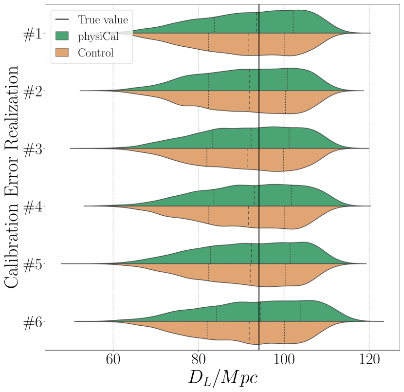
Figure 3: $D_{L}$ likelihood for the six scenarios, miscalibrated (green) vs. control (orange) runs, the vertical dashed lines mark the 25%, 50% and 75% percentiles.

Label	Miscalibrated	Control
#1	$-1.0\%$	$-2.5\%$
#2	$-2.3\%$	$-2.3\%$
#3	$-1.2\%$	$-2.1\%$
#4	$-0.9\%$	$-2.3\%$
#5	$-1.5\%$	$-2.5\%$
#6	$0.5\%$	$-2.6\%$

Table 1: $\Delta D_{L}$ in the likelihoods for PhysiCal runs with and without large CEs.

The results from using the PhysiCal and Spline methods for all three detectors agree very well. Thus, we only show the results from the PhysiCal methods in Fig. 3 and Tab. 1, and the ones from the Spline method in Appendix B.

Comparing with the control runs, where the offsets are between $-2.1\%$ to $-2.6\%$, the CE realization #6 leads to the most significant differences in the $D_{L}$ likelihoods. Thus, we apply it to the data of a hundred BNSs. We note the control runs all show a negative $\Delta D_{L}$; that can be explained by the well-known correlation between $D_{L}$ and inclination Chen et al. (2019). Since all sources in Fig. 3 have an inclination, $\iota$, of 30^∘, and the inclination prior goes like $\sin\iota$, we expect an offset towards larger inclination values, where the prior is larger, and thus smaller distances. This offset will no longer be present in the analysis of 100 events, since the 100 events have inclinations drawn from a uniform-in-cosine distribution (effectively $\sin\iota d\iota$), the same as the prior.

In Fig. 4, we vary the fraction of BNSs whose data are miscalibrated with CE realization #6 and plot the posterior distribution of the dimensionless $h_{0}$, defined as $H_{0}=h_{0}100~{}\mathrm{km\ s}^{-1}\mathrm{Mpc}^{-1}$. We assign CE #6 to $x\%$ of the BNS events, while the other events do not suffer from any miscalibration. The joint $h_{0}$ posterior starts to shift towards smaller values as we increase the fraction of BNSs affected by CE #6, and the posteriors exclude the true value of $h_{0}=0.679$ from the 90% CI when the data of more than 50% of the 100 BNSs are miscalibrated.

Figure 4: $h_{0}$ posteriors when we have different fractions of miscalibrated events. Thicker curves indicate results with more BNS events miscalibrated.

Next, we vary the total number of detected events besides varying the percentages of miscalibrated events. For $n$ detected events, we randomly miscalibrate $x\%$ of the $n$ events, and repeat the random draw for $\lfloor 100/n\rfloor$ trials (i.e. rounding down $100/n$ to an integer) for each pair of $\{n,x\}$. The number of trials is reduced as $n$ increases in order to keep each trial independent, and no event appears in more than one trial. We calculate the median and the bounds of 90% CI for each trial. In Fig. 5, the results are plotted for each pair of $\{n,x\}$; the green points are medians of the $\lfloor 100/n\rfloor$ medians from each trial, and the error bars are the medians of the 90% CI bounds from each trial. The orange points and error bars indicate the results for the control runs.

If 100% of the detected events suffer from miscalibration, the joint $h_{0}$ posterior excludes the true value from its 90% CI after 40 detections or more. When 50% of the detected BNSs suffer from miscalibration, the posterior only start to exclude the true $h_{0}$ after more than 90 events, and when 10% of the detected BNSs suffer from miscalibration, the posterior includes the true $h_{0}$ even after 100 detections. In the case of 100 detections, the results in Fig. 5 (the rightmost sets of points in each subplot) represent the same scenario as Fig. 4.

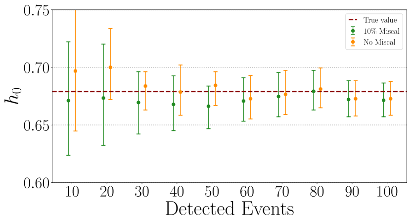
(a) 10% of the events miscalibrated.

(b) 50% of the events miscalibrated.

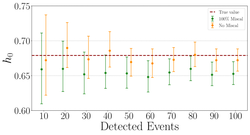
(c) 100% of the events miscalibrated.

Figure 5: $h_{0}$ posteriors when we have certain number of detections, plotted when 10%, 50% and 100% of the events are miscalibrated. We introduce an artificial offset on the x-axis for plotting purposes.

IV Conclusion

GW observations of EM-bright compact binary coalescences provide an independent way to measure the Hubble constant and to potentially break the existing tension between the early and late universe $H_{0}$ measurements. As we observe more of such events, the resulting $H_{0}$ posterior will be increasingly constraining, making it important to thoroughly control and understand potential systematic biases.

In this study, we artificially added large CEs to the GW data stream, and investigated their effects on the inference of $H_{0}$. Our analysis is constructed not to contain any systematic errors or statistical uncertainties from the EM observations like peculiar velocities Howlett and Davis (2020); Mukherjee et al. (2021b), or viewing angles Chen (2020), for our inference of $H_{0}$. Since we simulate and recover the GW signals with the same waveform family (IMRPhenomPv2), there are no waveform systematics present in our study either.

We found that the $H_{0}$ posterior does not exclude the true value from its 90% CI, corresponding to a 2–3% systematic error, unless we are inferring $H_{0}$ with more than 40 BNS detections that all suffer from the same large CEs. The total number of detections required increases to $\sim 90$ BNSs when 50% of them suffer from miscalibration. When 10% of BNSs are miscalibrated, the true value is not excluded even after 100 BNS detections. For comparison, systematic errors due to the EM observation side, for example kilonova viewing angles, will be 2% after 50 BNS detections Chen (2020).

All of the outliers $\{\eta^{\mathrm{out}}\}_{i}$ that motivate our study are based on modeled systematic error surrounding times of real physical changes or malfunctions in the O3 detectors. These events are generally rare and relatively short-lived; typically $<1\%$ of the time over any few-month observing period – the typical duration of stable detector configurations during an observing run Sun et al. (2020, 2021). In our analysis, we assume we only know and use $\{\eta^{\mathrm{typ}}\}_{i}$ to marginalize over CEs during PE, while $\{\eta^{\mathrm{out}}\}_{i}$, although resent through some fraction of detected BNS events, is assumed to be unknown and uncharacterized. There is a very low probability that a large CE remains uncharacterized over a period of many months during which dozens of BNSs are detected, given the current estimate of astrophysical event rate, $320^{+490}_{-240}\;\mathrm{Gpc}^{3}\mathrm{yr}^{-1}$ Collaboration and Collaboration (2021) vs. the few-month duration of stable detector configurations and the frequency of measurements during those periods.

Our results imply that CEs are not going to be significant concern in the measurement of the Hubble constant with the bright sirens method for the next many years. In the most realistic case, where large instances of CE like the ones described in this paper affect a small percent of the sources, CE will not become the limiting factor until more than 100 BNSs, each with an EM counterpart, have been found. Since the bright siren method is likely to provide the smallest statistical uncertainties, other approaches to constrain $H_{0}$ using distance measurements from GW sources are going to be even less sensitive to CEs.

In this work we have focused on the effect of CEs on inference results of BNSs. We will report on other types of compact binary coalescences, such as neutron star black hole mergers and binary black holes, as well as on the posteriors for calibration parameters from PhysiCal, in a forthcoming paper.

V Acknowledgments

Software: The authors acknowledge the use of the LIGO Algorithm Library LIGO Scientific Collaboration (2018), and specifically of the LALInference inference package Veitch et al. (2015), as released through conda anaconda. Plots were produced with matplotlib Hunter (2007). The authors acknowledge use of iPython Pérez and Granger (2007), NumPy Harris et al. (2020) and SciPy Virtanen et al. (2020). The authors are grateful for computational resources provided by the LIGO Laboratory and supported by National Science Foundation Grants PHY-0757058 and PHY-0823459. The authors would like to thank Jonathan Gair, Evan Goetz, Martin Hendry, Daniel Holz, Suvodip Mukherjee, Ethan Payne Jameson Graef Rollins, Nicola Tamanini, Paxton Turner, Madeline Wade, Alan J. Weinstein for useful discussions. Y. H., C.- J. H., S. V. acknowledge support of the National Science Foundation, and the LIGO Laboratory. LIGO was constructed by the California Institute of Technology and Massachusetts Institute of Technology with funding from the National Science Foundation and operates under cooperative agreement PHY-0757058. S. V.and Y. H. acknowledge support of the National Science Foundation trough the award PHY-2045740. Virgo is funded by the French Centre National de Recherche Scientifique (CNRS), the Italian Istituto Nazionale della Fisica Nucleare (INFN) and the Dutch Nikhef, with contributions by Polish and Hungarian institutes. H.-Y. C. is supported by NASA through NASA Hubble Fellowship grants No. HST-HF2-51452.001-A awarded by the Space Telescope Science Institute, which is operated by the Association of Universities for Research in Astronomy, Inc., for NASA, under contract NAS5-26555. L. S. acknowledges the support of the Australian Research Council Centre of Excellence for Gravitational Wave Discovery (OzGrav), Project No. CE170100004. This is LIGO Document Number DCC-P2100350.

Appendix A $\eta^{\mathrm{mis}}$, $\{\eta^{\mathrm{out}}\}$ and $\{\eta^{\mathrm{typ}}\}$ for other five scenarios

Here, in Fig. 6–10, we show the $\eta^{\mathrm{mis}}$, $\{\eta^{\mathrm{out}}\}$, and $\{\eta^{\mathrm{typ}}\}$ for the other five calibration outlier cases identified in O3.

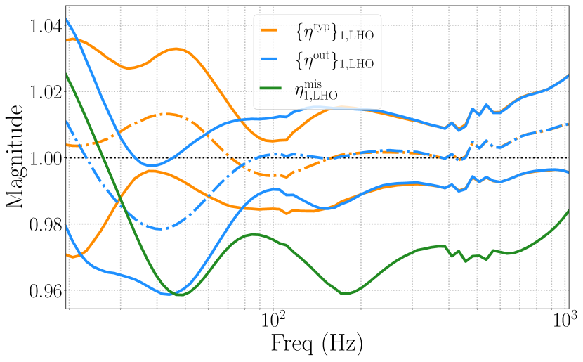
(a) Amplitude.

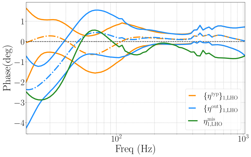
(b) Phase.

Figure 6: Time #1 of large amplitude and phase errors, $\{\eta^{\mathrm{out}}\}$ (blue), compared to the corresponding typical distribution, $\{\eta^{\mathrm{typ}}\}$ (orange), both showing the edges of the 1-$\sigma$ CIs in each frequency bin. Also plotted in green is the $\eta^{\mathrm{mis}}$ for this time.

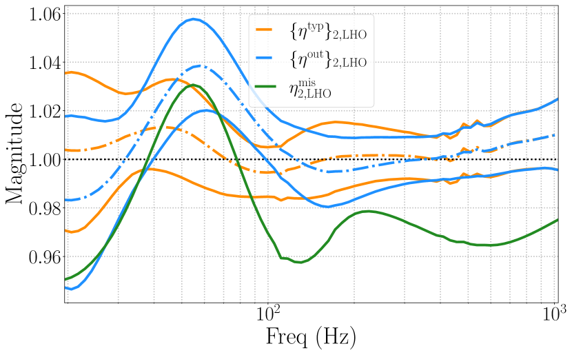
(a) Amplitude.

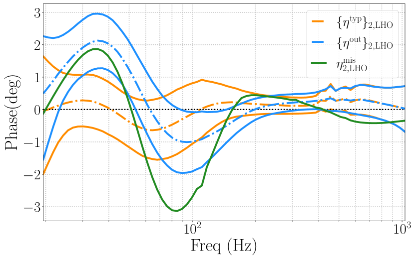
(b) Phase.

Figure 7: Time #2 of large amplitude and phase errors, $\{\eta^{\mathrm{out}}\}$ (blue), compared to the corresponding typical distribution, $\{\eta^{\mathrm{typ}}\}$ (orange), both showing the edges of the 1-$\sigma$ CIs in each frequency bin. Also plotted in green is the $\eta^{\mathrm{mis}}$ for this time.

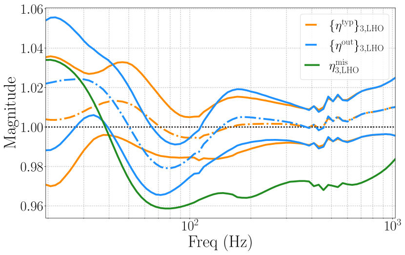
(a) Amplitude.

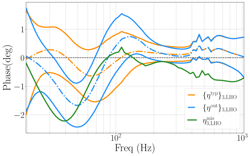
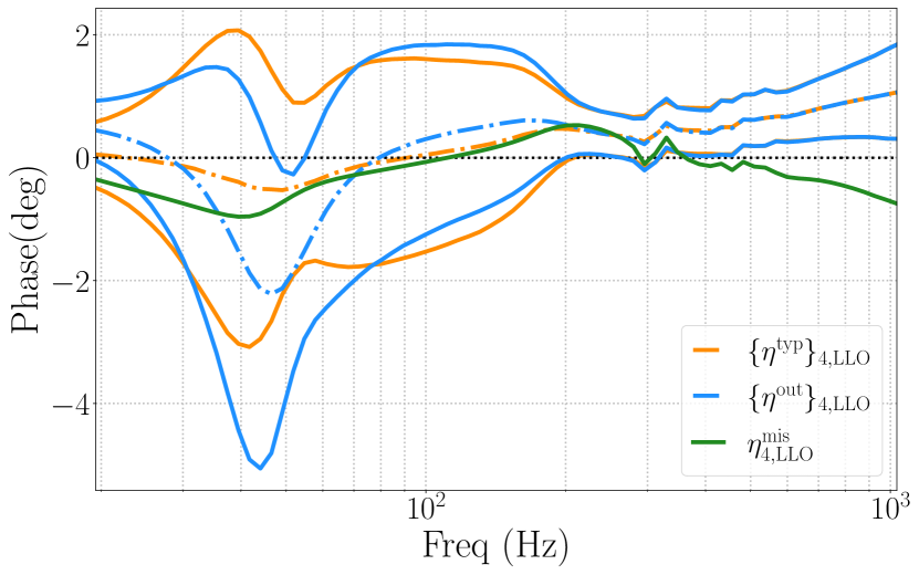
(b) Phase.

Figure 8: Time #3 of large amplitude and phase errors, $\{\eta^{\mathrm{out}}\}$ (blue), compared to the corresponding typical distribution, $\{\eta^{\mathrm{typ}}\}$ (orange), both showing the edges of the 1-$\sigma$ CIs in each frequency bin. Also plotted in green is the $\eta^{\mathrm{mis}}$ for this time.

(a) Amplitude.

(b) Phase.

Figure 9: Time #4 of large amplitude and phase errors, $\{\eta^{\mathrm{out}}\}$ (blue), compared to the corresponding typical distribution, $\{\eta^{\mathrm{typ}}\}$ (orange), both showing the edges of the 1-$\sigma$ CIs in each frequency bin. Also plotted in green is the $\eta^{\mathrm{mis}}$ for this time.

(a) Amplitude.

(b) Phase.

Figure 10: Time #5 of large amplitude and phase errors, $\{\eta^{\mathrm{out}}\}$ (blue), compared to the corresponding typical distribution, $\{\eta^{\mathrm{typ}}\}$ (orange), both showing the edges of the 1-$\sigma$ CIs in each frequency bin. Also plotted in green is the $\eta^{\mathrm{mis}}$ for this time.

Appendix B Spline Results

In Fig. 11, we show the distance likelihoods for BNSs at an SNR of 50, where the green and pink shaded distributions are obtained from the runs with the PhysiCal and Spline methods, respectively, both effected by the same $\eta^{\mathrm{mis}}$. We report $\Delta D_{L}$ in Tab. 2. The differences between the results are quite small compared to those between the PhysiCal runs with and without CEs.

Figure 11: $D_{L}$ likelihoods for the six scenarios, miscalibrated, PhysiCal (green) vs. Spline (pink) runs, the vertical dashed lines mark the 25%, 50% and 75% percentiles.

Label	PhysiCal	Spline
#1	$-0.8\%$	$-1.5\%$
#2	$-2.0\%$	$-2.6\%$
#3	$-1.6\%$	$-1.4\%$
#4	$-0.8$%	$-0.6\%$
#5	$-1.7\%$	$-1.2\%$
#6	$0.2\%$	$1.0\%$

Table 2: $\Delta D_{L}$ in the likelihoods for PhysiCal vs. Spline results.

References

- Abbott et al. (2018a) T. M. C. Abbott et al. (DES), Mon. Not. Roy. Astron. Soc. 480, 3879 (2018a), arXiv:1711.00403 [astro-ph.CO] .
- Aghanim et al. (2020) N. Aghanim et al. (Planck), Astron. Astrophys. 641, A6 (2020), arXiv:1807.06209 [astro-ph.CO] .
- Riess et al. (2016) A. G. Riess et al., Astrophys. J. 826, 56 (2016), arXiv:1604.01424 [astro-ph.CO] .
- Riess et al. (2018) A. G. Riess et al., Astrophys. J. 861, 126 (2018), arXiv:1804.10655 [astro-ph.CO] .
- Birrer et al. (2019) S. Birrer et al., Mon. Not. Roy. Astron. Soc. 484, 4726 (2019), arXiv:1809.01274 [astro-ph.CO] .
- Wong et al. (2020) K. C. Wong et al., Mon. Not. Roy. Astron. Soc. 498, 1420 (2020), arXiv:1907.04869 [astro-ph.CO] .
- Jang and Lee (2017) I. S. Jang and M. G. Lee, Astrophys. J. 836, 74 (2017), arXiv:1702.01118 [astro-ph.CO] .
- Freedman et al. (2019) W. L. Freedman et al., (2019), 10.3847/1538-4357/ab2f73, arXiv:1907.05922 [astro-ph.CO] .
- Kim et al. (2020) Y. J. Kim, J. Kang, M. G. Lee, and I. S. Jang, Astrophys. J. 905, 104 (2020), arXiv:2010.01364 [astro-ph.CO] .
- Schutz (1986) B. F. Schutz, Nature 323, 310 (1986).
- Holz and Hughes (2005) D. E. Holz and S. A. Hughes, Astrophys. J. 629, 15 (2005), arXiv:astro-ph/0504616 .
- Dalal et al. (2006) N. Dalal, D. E. Holz, S. A. Hughes, and B. Jain, Phys. Rev. D 74, 063006 (2006), arXiv:astro-ph/0601275 .
- Nissanke et al. (2010) S. Nissanke, D. E. Holz, S. A. Hughes, N. Dalal, and J. L. Sievers, Astrophys. J. 725, 496 (2010), arXiv:0904.1017 [astro-ph.CO] .
- Nissanke et al. (2013) S. Nissanke, D. E. Holz, N. Dalal, S. A. Hughes, J. L. Sievers, and C. M. Hirata, (2013), arXiv:1307.2638 [astro-ph.CO] .
- Chen et al. (2018) H.-Y. Chen, M. Fishbach, and D. E. Holz, Nature 562, 545 (2018), arXiv:1712.06531 [astro-ph.CO] .
- Hotokezaka et al. (2019) K. Hotokezaka, E. Nakar, O. Gottlieb, S. Nissanke, K. Masuda, G. Hallinan, K. P. Mooley, and A. T. Deller, Nature Astron. 3, 940 (2019), arXiv:1806.10596 [astro-ph.CO] .
- Soares-Santos et al. (2019) M. Soares-Santos et al. (DES, LIGO Scientific, Virgo), Astrophys. J. Lett. 876, L7 (2019), arXiv:1901.01540 [astro-ph.CO] .
- Feeney et al. (2021) S. M. Feeney, H. V. Peiris, S. M. Nissanke, and D. J. Mortlock, Phys. Rev. Lett. 126, 171102 (2021), arXiv:2012.06593 [astro-ph.CO] .
- Messenger and Read (2012) C. Messenger and J. Read, Phys. Rev. Lett. 108, 091101 (2012), arXiv:1107.5725 [gr-qc] .
- Del Pozzo et al. (2017) W. Del Pozzo, T. G. F. Li, and C. Messenger, Phys. Rev. D 95, 043502 (2017), arXiv:1506.06590 [gr-qc] .
- Dietrich et al. (2020) T. Dietrich, M. W. Coughlin, P. T. H. Pang, M. Bulla, J. Heinzel, L. Issa, I. Tews, and S. Antier, Science 370, 1450 (2020), arXiv:2002.11355 [astro-ph.HE] .
- Del Pozzo (2012) W. Del Pozzo, Phys. Rev. D 86, 043011 (2012), arXiv:1108.1317 [astro-ph.CO] .
- Abbott et al. (2021) B. P. Abbott et al. (LIGO Scientific, Virgo), Astrophys. J. 909, 218 (2021), arXiv:1908.06060 [astro-ph.CO] .
- Gray et al. (2020) R. Gray et al., Phys. Rev. D 101, 122001 (2020), arXiv:1908.06050 [gr-qc] .
- Taylor et al. (2012) S. R. Taylor, J. R. Gair, and I. Mandel, Phys. Rev. D 85, 023535 (2012), arXiv:1108.5161 [gr-qc] .
- Farr et al. (2019) W. M. Farr, M. Fishbach, J. Ye, and D. Holz, Astrophys. J. Lett. 883, L42 (2019), arXiv:1908.09084 [astro-ph.CO] .
- Mastrogiovanni et al. (2021) S. Mastrogiovanni, K. Leyde, C. Karathanasis, E. Chassande-Mottin, D. A. Steer, J. Gair, A. Ghosh, R. Gray, S. Mukherjee, and S. Rinaldi, Phys. Rev. D 104, 062009 (2021), arXiv:2103.14663 [gr-qc] .
- Finke et al. (2021) A. Finke, S. Foffa, F. Iacovelli, M. Maggiore, and M. Mancarella, JCAP 08, 026 (2021), arXiv:2101.12660 [astro-ph.CO] .
- Mukherjee et al. (2021a) S. Mukherjee, B. D. Wandelt, S. M. Nissanke, and A. Silvestri, Phys. Rev. D 103, 043520 (2021a), arXiv:2007.02943 [astro-ph.CO] .
- Diaz and Mukherjee (2021) C. C. Diaz and S. Mukherjee, (2021), arXiv:2107.12787 [astro-ph.CO] .
- Abbott et al. (2018b) B. P. Abbott et al. (KAGRA, LIGO Scientific, VIRGO), Living Rev. Rel. 21, 3 (2018b), arXiv:1304.0670 [gr-qc] .
- Barsotti et al. (2018) L. Barsotti, P. Fritschel, M. Evans, and S. Gras, Updated Advanced LIGO sensitivity design curve, Tech. Rep. LIGO-T1800044 (LIGO Laboratory, 2018).
- Collaboration (2015) T. L. S. Collaboration, Classical and Quantum Gravity 32, 074001 (2015).
- Tse et al. (2019) M. Tse, H. Yu, N. Kijbunchoo, A. Fernandez-Galiana, P. Dupej, L. Barsotti, C. D. Blair, D. D. Brown, S. E. Dwyer, A. Effler, M. Evans, P. Fritschel, V. V. Frolov, A. C. Green, G. L. Mansell, F. Matichard, N. Mavalvala, D. E. McClelland, L. McCuller, T. McRae, J. Miller, A. Mullavey, E. Oelker, I. Y. Phinney, D. Sigg, B. J. J. Slagmolen, T. Vo, R. L. Ward, C. Whittle, R. Abbott, C. Adams, R. X. Adhikari, A. Ananyeva, S. Appert, K. Arai, J. S. Areeda, Y. Asali, S. M. Aston, C. Austin, A. M. Baer, M. Ball, S. W. Ballmer, S. Banagiri, D. Barker, J. Bartlett, B. K. Berger, J. Betzwieser, D. Bhattacharjee, G. Billingsley, S. Biscans, R. M. Blair, N. Bode, P. Booker, R. Bork, A. Bramley, A. F. Brooks, A. Buikema, C. Cahillane, K. C. Cannon, X. Chen, A. A. Ciobanu, F. Clara, S. J. Cooper, K. R. Corley, S. T. Countryman, P. B. Covas, D. C. Coyne, L. E. H. Datrier, D. Davis, C. Di Fronzo, J. C. Driggers, T. Etzel, T. M. Evans, J. Feicht, P. Fulda, M. Fyffe, J. A. Giaime, K. D. Giardina, P. Godwin, E. Goetz, S. Gras, C. Gray, R. Gray, A. Gupta, E. K. Gustafson, R. Gustafson, J. Hanks, J. Hanson, T. Hardwick, R. K. Hasskew, M. C. Heintze, A. F. Helmling-Cornell, N. A. Holland, J. D. Jones, S. Kandhasamy, S. Karki, M. Kasprzack, K. Kawabe, P. J. King, J. S. Kissel, R. Kumar, M. Landry, B. B. Lane, B. Lantz, M. Laxen, Y. K. Lecoeuche, J. Leviton, J. Liu, M. Lormand, A. P. Lundgren, R. Macas, M. MacInnis, D. M. Macleod, S. Márka, Z. Márka, D. V. Martynov, K. Mason, T. J. Massinger, R. McCarthy, S. McCormick, J. McIver, G. Mendell, K. Merfeld, E. L. Merilh, F. Meylahn, T. Mistry, R. Mittleman, G. Moreno, C. M. Mow-Lowry, S. Mozzon, T. J. N. Nelson, P. Nguyen, L. K. Nuttall, J. Oberling, R. J. Oram, B. O’Reilly, C. Osthelder, D. J. Ottaway, H. Overmier, J. R. Palamos, W. Parker, E. Payne, A. Pele, C. J. Perez, M. Pirello, H. Radkins, K. E. Ramirez, J. W. Richardson, K. Riles, N. A. Robertson, J. G. Rollins, C. L. Romel, J. H. Romie, M. P. Ross, K. Ryan, T. Sadecki, E. J. Sanchez, L. E. Sanchez, T. R. Saravanan, R. L. Savage, D. Schaetzl, R. Schnabel, R. M. S. Schofield, E. Schwartz, D. Sellers, T. J. Shaffer, J. R. Smith, S. Soni, B. Sorazu, A. P. Spencer, K. A. Strain, L. Sun, M. J. Szczepańczyk, M. Thomas, P. Thomas, K. A. Thorne, K. Toland, C. I. Torrie, G. Traylor, A. L. Urban, G. Vajente, G. Valdes, D. C. Vander-Hyde, P. J. Veitch, K. Venkateswara, G. Venugopalan, A. D. Viets, C. Vorvick, M. Wade, J. Warner, B. Weaver, R. Weiss, B. Willke, C. C. Wipf, L. Xiao, H. Yamamoto, M. J. Yap, H. Yu, L. Zhang, M. E. Zucker, and J. Zweizig, Phys. Rev. Lett. 123, 231107 (2019).
- Abbott et al. (2017a) B. P. Abbott et al. (LIGO Scientific, Virgo, 1M2H, Dark Energy Camera GW-E, DES, DLT40, Las Cumbres Observatory, VINROUGE, MASTER), Nature 551, 85 (2017a), arXiv:1710.05835 [astro-ph.CO] .
- Abbott et al. (2017b) B. P. Abbott et al. (LIGO Scientific, Virgo, Fermi-GBM, INTEGRAL), Astrophys. J. Lett. 848, L13 (2017b), arXiv:1710.05834 [astro-ph.HE] .
- Abbott et al. (2017c) B. P. Abbott et al. (LIGO Scientific, Virgo), Phys. Rev. Lett. 119, 161101 (2017c), arXiv:1710.05832 [gr-qc] .
- Abbott et al. (2017d) B. P. Abbott et al. (LIGO Scientific, Virgo, Fermi GBM, INTEGRAL, IceCube, AstroSat Cadmium Zinc Telluride Imager Team, IPN, Insight-Hxmt, ANTARES, Swift, AGILE Team, 1M2H Team, Dark Energy Camera GW-EM, DES, DLT40, GRAWITA, Fermi-LAT, ATCA, ASKAP, Las Cumbres Observatory Group, OzGrav, DWF (Deeper Wider Faster Program), AST3, CAASTRO, VINROUGE, MASTER, J-GEM, GROWTH, JAGWAR, CaltechNRAO, TTU-NRAO, NuSTAR, Pan-STARRS, MAXI Team, TZAC Consortium, KU, Nordic Optical Telescope, ePESSTO, GROND, Texas Tech University, SALT Group, TOROS, BOOTES, MWA, CALET, IKI-GW Follow-up, H.E.S.S., LOFAR, LWA, HAWC, Pierre Auger, ALMA, Euro VLBI Team, Pi of Sky, Chandra Team at McGill University, DFN, ATLAS Telescopes, High Time Resolution Universe Survey, RIMAS, RATIR, SKA South Africa/MeerKAT), Astrophys. J. Lett. 848, L12 (2017d), arXiv:1710.05833 [astro-ph.HE] .
- Abbott et al. (2019) B. P. Abbott et al. (LIGO Scientific, Virgo), Phys. Rev. X 9, 011001 (2019), arXiv:1805.11579 [gr-qc] .
- Hall et al. (2019) E. D. Hall, C. Cahillane, K. Izumi, R. J. E. Smith, and R. X. Adhikari, Class. Quant. Grav. 36, 205006 (2019), arXiv:1712.09719 [astro-ph.IM] .
- Sun et al. (2020) L. Sun et al., Class. Quant. Grav. 37, 225008 (2020), arXiv:2005.02531 [astro-ph.IM] .
- Sun et al. (2021) L. Sun et al., ArXiv e-prints (2021), arXiv:2107.00129 [astro-ph.IM] .
- Vitale et al. (2012) S. Vitale, W. Del Pozzo, T. G. F. Li, C. Van Den Broeck, I. Mandel, B. Aylott, and J. Veitch, Phys. Rev. D 85, 064034 (2012), arXiv:1111.3044 [gr-qc] .
- Payne et al. (2020) E. Payne, C. Talbot, P. D. Lasky, E. Thrane, and J. S. Kissel, Phys. Rev. D 102, 122004 (2020), arXiv:2009.10193 [astro-ph.IM] .
- Vitale et al. (2021) S. Vitale, C.-J. Haster, L. Sun, B. Farr, E. Goetz, J. Kissel, and C. Cahillane, Phys. Rev. D 103, 063016 (2021), arXiv:2009.10192 [gr-qc] .
- Essick and Holz (2019) R. Essick and D. E. Holz, Class. Quant. Grav. 36, 125002 (2019), arXiv:1902.08076 [astro-ph.IM] .
- Schutz and Sathyaprakash (2020) B. F. Schutz and B. S. Sathyaprakash, ArXiv e-prints (2020), arXiv:2009.10212 [gr-qc] .
- Husa et al. (2016) S. Husa, S. Khan, M. Hannam, M. Pürrer, F. Ohme, X. Jiménez Forteza, and A. Bohé, Phys. Rev. D 93, 044006 (2016), arXiv:1508.07250 [gr-qc] .
- Khan et al. (2016) S. Khan, S. Husa, M. Hannam, F. Ohme, M. Pürrer, X. Jiménez Forteza, and A. Bohé, Phys. Rev. D 93, 044007 (2016), arXiv:1508.07253 [gr-qc] .
- Hannam et al. (2014) M. Hannam, P. Schmidt, A. Bohé, L. Haegel, S. Husa, F. Ohme, G. Pratten, and M. Pürrer, Phys. Rev. Lett. 113, 151101 (2014), arXiv:1308.3271 [gr-qc] .
- Smith et al. (2016) R. Smith, S. E. Field, K. Blackburn, C.-J. Haster, M. Pürrer, V. Raymond, and P. Schmidt, Phys. Rev. D 94, 044031 (2016), arXiv:1604.08253 [gr-qc] .
- Ohme et al. (2013) F. Ohme, A. B. Nielsen, D. Keppel, and A. Lundgren, Phys. Rev. D 88, 042002 (2013), arXiv:1304.7017 [gr-qc] .
- Berry et al. (2015) C. P. L. Berry et al., Astrophys. J. 804, 114 (2015), arXiv:1411.6934 [astro-ph.HE] .
- Samajdar and Dietrich (2018) A. Samajdar and T. Dietrich, Phys. Rev. D 98, 124030 (2018), arXiv:1810.03936 [gr-qc] .
- Buikema et al. (2020) A. Buikema, C. Cahillane, G. Mansell, C. Blair, R. Abbott, C. Adams, R. Adhikari, A. Ananyeva, S. Appert, K. Arai, et al., Physical Review D 102, 062003 (2020).
- Acernese et al. (2014) F. a. Acernese, M. Agathos, K. Agatsuma, D. Aisa, N. Allemandou, A. Allocca, J. Amarni, P. Astone, G. Balestri, G. Ballardin, et al., Classical and Quantum Gravity 32, 024001 (2014).
- Viets et al. (2018) A. Viets et al., Class. Quant. Grav. 35, 095015 (2018), arXiv:1710.09973 [astro-ph.IM] .
- Abbott et al. (2017e) B. P. Abbott et al. (LIGO Scientific), Phys. Rev. D 95, 062003 (2017e), arXiv:1602.03845 [gr-qc] .
- Tuyenbayev et al. (2017) D. Tuyenbayev et al., Class. Quant. Grav. 34, 015002 (2017), arXiv:1608.05134 [astro-ph.IM] .
- Vallisneri (2008) M. Vallisneri, Phys. Rev. D 77, 042001 (2008), arXiv:gr-qc/0703086 .
- Veitch et al. (2015) J. Veitch et al., Phys. Rev. D 91, 042003 (2015), arXiv:1409.7215 [gr-qc] .
- Abbott et al. (2016) B. P. Abbott et al. (LIGO Scientific, Virgo), Phys. Rev. Lett. 116, 241102 (2016), arXiv:1602.03840 [gr-qc] .
- Vitale et al. (2020) S. Vitale, D. Gerosa, W. M. Farr, and S. R. Taylor, ArXiv e-prints (2020), arXiv:2007.05579 [astro-ph.IM] .
- Zimmerman et al. (2019) A. Zimmerman, C.-J. Haster, and K. Chatziioannou, Phys. Rev. D 99, 124044 (2019), arXiv:1903.11008 [astro-ph.IM] .
- Farr et al. (2014) W. Farr, B. Farr, and T. Littenberg, Updated Advanced LIGO sensitivity design curve, Tech. Rep. LIGO-T1400682 (LIGO Laboratory, 2014).
- Chen et al. (2019) H.-Y. Chen, S. Vitale, and R. Narayan, Phys. Rev. X 9, 031028 (2019), arXiv:1807.05226 [astro-ph.HE] .
- Howlett and Davis (2020) C. Howlett and T. M. Davis, Mon. Not. Roy. Astron. Soc. 492, 3803 (2020), arXiv:1909.00587 [astro-ph.CO] .
- Mukherjee et al. (2021b) S. Mukherjee, G. Lavaux, F. R. Bouchet, J. Jasche, B. D. Wandelt, S. M. Nissanke, F. Leclercq, and K. Hotokezaka, Astron. Astrophys. 646, A65 (2021b), arXiv:1909.08627 [astro-ph.CO] .
- Chen (2020) H.-Y. Chen, Phys. Rev. Lett. 125, 201301 (2020), arXiv:2006.02779 [astro-ph.HE] .
- Collaboration and Collaboration (2021) L. S. Collaboration and V. Collaboration (LIGO Scientific Collaboration and Virgo Collaboration), Phys. Rev. X 11, 021053 (2021).
- LIGO Scientific Collaboration (2018) LIGO Scientific Collaboration, “LIGO Algorithm Library - LALSuite,” free software (GPL) (2018).
- Hunter (2007) J. D. Hunter, Computing in Science & Engineering 9, 90 (2007).
- Pérez and Granger (2007) F. Pérez and B. E. Granger, Computing in Science and Engineering 9, 21 (2007).
- Harris et al. (2020) C. R. Harris et al., Nature 585, 357 (2020), arXiv:2006.10256 [cs.MS] .
- Virtanen et al. (2020) P. Virtanen et al., Nature Meth. 17, 261 (2020), arXiv:1907.10121 [cs.MS] .