Unified Contrastive Learning in Image-Text-Label Space

Abstract

Visual recognition is recently learned via either supervised learning on human-annotated image-label data or language-image contrastive learning with webly-crawled image-text pairs. While supervised learning may result in a more discriminative representation, language-image pretraining shows unprecedented zero-shot recognition capability, largely due to the different properties of data sources and learning objectives. In this work, we introduce a new formulation by combining the two data sources into a common image-text-label space. In this space, we propose a new learning paradigm, called Unified Contrastive Learning (UniCL) with a single learning objective to seamlessly prompt the synergy of two data types. Extensive experiments show that our UniCL is an effective way of learning semantically rich yet discriminative representations, universally for image recognition in zero-shot, linear-probing, fully finetuning and transfer learning scenarios. Particularly, it attains gains up to 9.2% and 14.5% in average on zero-shot recognition benchmarks over the language-image contrastive learning and supervised learning methods, respectively. In linear probe setting, it also boosts the performance over the two methods by 7.3% and 3.4%, respectively. Our study also indicates that UniCL stand-alone is a good learner on pure image-label data, rivaling the supervised learning methods across three image classification datasets and two types of vision backbones, ResNet and Swin Transformer. Code is available at: https://github.com/microsoft/UniCL.

1 Introduction

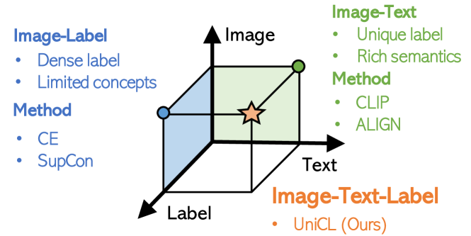
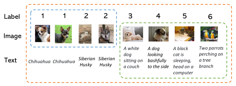
Figure 1: Unified contrastive learning paradigm in the image-text-label space, which recovers the supervised learning (e.g., Cross-Entropy (CE) [47] or Supervised Contrastive Learning (SupCon) [30]) on image-label data, and language-image contrastive learning (e.g., CLIP [48] or ALIGN [29]) on image-text data.

Learning to recognize visual concepts in an image has been a fundamental and long-standing research problem. Typically, this can be tackled via either supervised learning on human-annotated image-label pairs [10] or contrastive learning on webly-crawed image-text pairs [48, 29]. When fueled with clean and large-scale human-annotated image-label data, e.g., ImageNet [10], supervised learning can attain decent visual recognition capacities over the given categories [35, 55, 23] and also powerful transfer learning abilities [14, 33]. Nevertheless, collecting precise image-label data can be a laborious and expensive process, not to say its difficulty to scale up to numerous visual concepts. On the other hand, language-image contrastive learning has recently emerged as a promising approach by leveraging huge amounts of webly-crawled image-text pairs. These pairs are usually noisy, free-form but cover lots of visual concepts. As demonstrated in CLIP [48] and ALIGN [29], models learned from hundreds of millions of image-text pairs can attain impressive low-shot recognition performance for a wide range of visual understanding scenarios. Though these image-text models show a broad coverage of visual concepts, we find in our experiments that they usually lack the strong discriminative ability required by transfer learning. A natural question is: can we have one model for both discriminative representations and broad visual concept coverage?

In this work, we take the first step to answer this question. We start with a new perspective, illustrated in Fig. 1. Instead of isolating image-label and image-text data, we define an image-text-label space and show how we can eliminate the boundary between two data types. As shown in Fig. 1 left part, supervised learning  [30] on image-label data typically aims at mapping images to discrete labels, and completely ignores the textual concept associated with each label during the training. In contrast, language-image contrastive learning [48] aims at learning a pair of visual and textual encoders to align images and texts as shown in Fig. 1 right part. This learning method implicitly assumes that each image-text pair has a unique label. Comparing these two learning paradigms side by side, we can see that both of them actually reside in the common image-text-label space, which is constructed by mapping each label to a textual concept for supervised learning, and assigning each textual description a unique label for language-image pretraining, as shown in Fig. 1 bottom. Based on this new perspective, we can simply use a visual encoder and a language encoder to encode the images and texts, and align the visual and textual features with the guide of labels (unique labels for image-text pairs and manual labels for image-label data). However, learning from these combined labels cannot be supported in existing supervised learning and language-image contrastive learning paradigms. For this purpose, we propose a unified contrastive learning method, called UniCL to seamlessly accommodate both data types for visual-semantic representation learning. It takes images, texts as input and compute the loss with softened targets derived from the labels. With UniCL, we combine image-label and image-text data together to learn discriminative and semantic-rich representations, which are beneficial to a variety of downstream tasks. To summarize, our main contributions are:

• We introduce a new perspective of image-text-label space, which can seamlessly unify the commonly used image-label and image-text data.

• We propose a unified contrastive learning method called UniCL in the image-text-label space, that can learn from either of the image-label and image-text data, or both.

• Extensive experiments show that our UniCL can leverage both types of data effectively and achieve superior performance universally on standard zero-shot, linear probe, fully-finetuning and transfer learning settings.

Finally, we scaled up UniCL to billions of image-text-label data in Florence [72] and demonstrated its superiority over CLIP [48] and ALIGN [29] across dozens of benchmarks. Hereby, we highly recommend UniCL as a generic multi-modal learning paradigm for vision.

2 Related works

Supervised Learning. Supervised learning for image classification has a long history. As mentioned earlier, a canonical way of supervised learning is mapping images to manual labels. With this goal, numerous works have pushed the image recognition performance from different directions, such as data scale from MNIST [37] to ImageNet-1K [10], model architectures from convolutional neural networks (CNNs) [36, 35, 41, 54, 23, 26, 55] to Transformers [15, 64, 44, 59, 67, 76, 71], and learning objectives from original Cross-Entropy [47] to marginal losses [43, 11, 52] and recent supervised contrastive loss [30]. In this paper, we develop a unified contrastive learning method that regards image-label as image-text-label data to learn a generic visual-semantic space. It calls back the textual concepts behind the labels and use them as a special format of language. In this sense, our work is also related to conventional zero-shot classification [9, 69, 46, 65, 28, 70]. Most of these works pay attention to recognize fine-grained categories at a small scale. Our work goes beyond such restricted setting and is targeted to learn a good and rich visual-semantic representation from the combined image-label and image-text pairs.

Language-Image Contrastive Learning. Vision-and-language is a rapidly growing field. Existing works can be broadly categorized into two classes. $(i)$ Inspired by the success of BERT [13], the first line of research focuses on learning generic multi-modal fusion layers based on masked token prediction and/or image-text matching, given the pre-extracted features from visual and textual encoder [17, 45, 40, 53, 77, 31, 39, 66]. They aim to improve downstream tasks such as visual question answering [2, 27], image captioning [42, 1], visual commonsense reasoning [74]. $(ii)$ Another line of works focuses on learning transferable visual representation from natural language supervisions, including generative [50, 12] and contrastive methods [16, 63, 62, 78, 48, 29]. Recently, contrastive learning has been scaled up in representative works such as CLIP [48] and ALIGN [29], by pretraining on hundreds of millions of webly-crawled image-text pairs. Our work is close to these works in that we also use the image-text data as one of the major data sources. However, image-label data is ignored in these works. Our work presents the first unified contrastive learning method that can seamlessly leverage both.

Self-supervised Learning. Self-supervised learning (SSL) for vision aims to learn general-purpose visual representations from raw pixels without supervisions from label or text [19]. Contrastive learning has laid the foundation for the best performing SSL models [57, 24, 6, 21, 3, 58, 8]. It maximizes agreement of learned representations between differently augmented views of the same image, and minimizes agreement of views from different images. This augmented-view-based paradigm has also been extended to non-contrastive methods [20, 7, 4, 38], where only positive image view pairs are considered in learning. Though image SSL has great promises in leveraging nearly infinite amounts of unlabelled image data in training [18], the lack of language association renders it hardly applicable to zero-shot recognition. Nevertheless, the success of contrastive learning in SSL has inspired the generalization of this methodology to a much broader range, such as CLIP [48] in image-text setting and our UniCL in image-text-label setting, where images and language descriptions can be considered as multi-modal views of the same underlying concepts.

3 Method

3.1 Preliminaries

Problem setup.

We define a triplet-wise data format $\mathcal{S}=\{(\boldsymbol{x}_{n},{\boldsymbol{t}}_{n},y_{n})\}_{n=1}^{N}$, where $\boldsymbol{x}\in\mathcal{X}$ is the image, and ${\boldsymbol{t}}\in\mathcal{T}$ is its corresponding language description (ranging from simple tokens such as category names to free-form text sequences), and $y\in\mathcal{Y}$ is a label indicating the index of the grouped or unique language description in the dataset. As we discussed earlier, this triplet data representation is a general format of widely existing image data, including the commonly used image-text and image-label data. On one hand, image-text pairs $\{(\boldsymbol{x}_{n},{\boldsymbol{t}}_{n})\}_{n=1}^{N}$ from the web usually have an one-to-one mapping, thus each image-text pair has unique label and $\mathcal{S}$ reduces to $\{(\boldsymbol{x}_{n},{\boldsymbol{t}}_{n},y_{n}\equiv n)\}_{n=1}^{N}$. On the other hand, though an image classification problem often uses simple category labels or indices, each label is induced from the similarity of concepts in its task definition [10]. Therefore, for image-label data, $\mathcal{S}$ reduces to $\{(\boldsymbol{x}_{n},{\boldsymbol{t}}_{n}\equiv C[y_{n}],y_{n})\}_{n=1}^{N}$, with $C$ as the set of concept names indexed by $y_{n}$. Based on this definition, we can represent an image-label pair as a labeled image-text pair, while an image-text pair as ones with unique label. An example of how they are unified is illustrated in Fig. 2. The goal of this work is to learn from the joint data $\mathcal{S}$, believing that the rich semantics in language description ${\boldsymbol{t}}$ and structured organizations of labels $y$ together are beneficial for learning semantic-rich and discriminative visual representations of images $\boldsymbol{x}$.

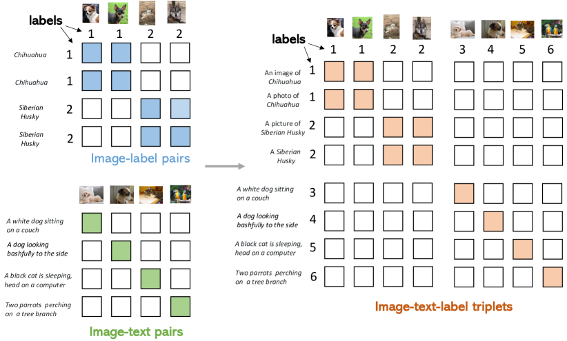
Figure 2: An illustration of covering image-label and image-text data in the image-text-label space. For image-label data, we associate a textual concept to each label, and the images and textual concepts are matched based on the annotated labels (blue tiles). For image-text data, each pair have unique label index, thus matched only at the diagonal entries (green tiles). On the right side, we can simply combine them as image-text-label triplets, and the red tiles means positive pairs while the blank tiles are negative pairs.

3.2 Unified Image-Text-Label Contrast

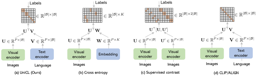
Figure 3: Illustrative comparisons across different learning paradigms. For a batch of size $|\mathcal{B}|$, all image features ${{\bf U}}$, ${{\bf U}}^{\prime}$ and text features ${{\bf V}}$ are in dimension $P$, and $K$ is the number of classes. Given a similarity matrix in each method, the labels play the role of defining the positive pairs whose elements are in orange, negatives are in white; CLIP has the one-to-one assumption for an image-text pair, which implicitly define the diagonal elements as positives.

For each image $\boldsymbol{x}$, an image encoder model $f_{\boldsymbol{\theta}}$ parameterized by $\boldsymbol{\theta}$ first represents $\boldsymbol{x}$ as a visual feature vector $\tilde{\boldsymbol{v}}\in\mathbb{R}^{d\times 1}$: $\tilde{\boldsymbol{v}}=f_{\boldsymbol{\theta}}(\boldsymbol{x})$. For each language description ${\boldsymbol{t}}\in\mathcal{T}$, we encode it with a text encoder $f_{\boldsymbol{\phi}}({\boldsymbol{t}})$ parameterized by $\boldsymbol{\phi}$ to get its feature vector $\tilde{\boldsymbol{u}}\in\mathbb{R}^{d\times 1}:\tilde{\boldsymbol{u}}=f_{\boldsymbol{\phi}}({\boldsymbol{t}})$. For $i$-th image $\boldsymbol{x}_{i}$ and $j$-th language description ${\boldsymbol{t}}_{j}$ in a batch $\mathcal{B}$, we normalize their feature vector to a hyper-sphere using $\boldsymbol{u}_{i}=\frac{f_{\boldsymbol{\theta}}(\boldsymbol{x}_{i})}{\|f_{\boldsymbol{\theta}}(\boldsymbol{x}_{i})\|}$ and $\boldsymbol{v}_{j}=\frac{f_{\boldsymbol{\phi}}({\boldsymbol{t}}_{j})}{\|f_{\boldsymbol{\phi}}({\boldsymbol{t}}_{j})\|}$, and their similarity is calculated as $s_{ij}=\boldsymbol{u}_{i}^{T}\boldsymbol{v}_{j}$. We consider a bidirectional learning objective between images and language:

$$\min_{\{\boldsymbol{\theta},\boldsymbol{\phi}\}}~{}~{}\mathcal{L}_{BiC}= \mathcal{L}_{i2t}+\mathcal{L}_{t2i},$$ (1)

including two contrastive terms (A temperature hyper-parameter $\tau$ controls the strength of penalties on hard negative samples):

• The image-to-text contrastive loss to align matched images in a batch with a given text

  $$\small\vspace{-4mm}\mathcal{L}_{i2t}= -\sum_{i\in\mathcal{B}}\frac{1}{|\mathcal{P}(i)|}\sum_{k\in\mathcal{P}(i)}\log\frac{\exp(\tau\boldsymbol{u}_{i}^{T}\boldsymbol{v}_{k})}{\sum_{j\in\mathcal{B}}\exp(\tau\boldsymbol{u}_{i}^{T}\boldsymbol{v}_{j})}$$ (2)

  where $k\in\mathcal{P}(i)=\{k|k\in\mathcal{B},y_{k}=y_{i}\}$.

• The text-to-image contrastive loss to align matched texts to a given image

  $$\small\vspace{-4mm}\mathcal{L}_{t2i}= -\sum_{j\in\mathcal{B}}\frac{1}{|\mathcal{P}(j)|}\sum_{k\in\mathcal{P}(j)}\log\frac{\exp(\tau\boldsymbol{u}_{k}^{T}\boldsymbol{v}_{j})}{\sum_{i\in\mathcal{B}}\exp(\tau\boldsymbol{u}_{i}^{T}\boldsymbol{v}_{j})}$$ (3)

  where $k\in\mathcal{P}(j)=\{k|k\in\mathcal{B},y_{k}=y_{j}\}$.

Using Fig. 2 right side as an example, the $\mathcal{L}_{i2t}$ is computed for each row, and $\mathcal{L}_{t2i}$ computed for each column. The red tiles indicate the positive pairs while blank tiles the negative ones, all allocated based on the labels.

3.3 Discussions & Properties

We discuss the unique properties of our proposed UniCL and build the connections with previous commonly used learning paradigms. An illustrative comparison is shown in Fig. 3, with more detailed analysis below.

Connections to Cross-Entropy [47] We note the proposed $\mathcal{L}_{BiC}$ in (1) is closely related to the standard cross-entropy loss used in supervised image classification. Specifically, the text-to-image contrastive term in (3) recovers cross-entropy as a special case, when the following conditions are satisfied: $(i)$ the text encoder $f_{\boldsymbol{\phi}}$ is represented as a simple linear embedding layer ${{\bf W}}$ with a bias $b$. $(ii)$ The batch size $|\mathcal{B}|$ is sufficiently larger than the number of classes $K$, so that all the class embedding vectors are used in contrastive learning, when stochastic sampling is used for training. $(iii)$ $\tau=1$, and $\ell_{2}$ normalization is excluded, so that $\tilde{\boldsymbol{u}}=\boldsymbol{u}$ and $\tilde{\boldsymbol{v}}=\boldsymbol{v}$. In this case, Eq. (3) becomes:

$$\small\min_{\{\boldsymbol{\theta},{{\bf W}}\}}~{}~{}\mathcal{L}_{CE}=\sum_{j\in\mathcal{B}}\log\frac{\exp(\boldsymbol{w}_{\hat{y}}\tilde{\boldsymbol{v}}_{j}+b_{\hat{y}})}{\sum_{k=1}^{K}\exp(\boldsymbol{w}_{k}\tilde{\boldsymbol{v}}_{j}+b_{k})}$$ (4)

where $\hat{y}$ is the ground-truth label for the $j$-th image in the batch. Based on this, we argue that $\mathcal{L}_{BiC}$ is more general than $\mathcal{L}_{CE}$, from two aspects: $(i)$ Augmentation with $\mathcal{L}_{i2t}$. The additional text-to-image term $\mathcal{L}_{i2t}$ in $\mathcal{L}_{BiC}$ plays the role of regularizer. Given a language description ${\boldsymbol{t}}_{j}$, all image features with the same ${\boldsymbol{t}}_{j}$ in the batch are clustered towards the text feature; otherwise they are pushed away. This can help prevent over-fitting, as demonstrated in our experiment later; $(ii)$ Text encoder $f_{\boldsymbol{\phi}}$. The text encoder can be specified as in more powerful forms such as 12-layer Transformers or pretrained BERT encoder, and take free-form text inputs beyond the set of category names.

Connections to SupCon [30] One shared property between our UniCL and SupCon is that both methods exploit label-guided contrastive learning: For any query, both methods leverage samples with the same label to contribute to the numerator as positives. Note that SupCon is proposed in the image-label setting, where each image is augmented with two different views. UniCL and SupCon differ in two aspects: $(i)$ Query-vs-Key modality. In SupCon, both query and key in contrastive learning are from the same modality: image-and-image pairs; In UniCL, the query and key are different modalities: image-and-language pairs. $(ii)$ Encoders. Only one shared image encoder is used in SupCon for query and key. Two different encoders are used in UniCL for different modalities, as shown in Fig. 3.

Connections to CLIP [48] For image-texts pairs, there are only one-to-one mappings between an image and its paired text in a batch. In another word, $\mathcal{P}(i)=\{i\}$ and $\mathcal{P}(j)=\{j\}$ for Eq. (2) and Eq. (3), respectively. Then $\mathcal{L}_{BiC}$ becomes:

• The image-to-text contrastive loss

  $$\small\mathcal{L}_{i2t}= -\sum_{i\in\mathcal{B}}\log\frac{\exp(\tau\boldsymbol{u}_{i}\boldsymbol{v}_{i})}{\sum_{j\in\mathcal{B}}\exp(\tau\boldsymbol{u}_{i}\boldsymbol{v}_{j})}$$ (5)

• The text-to-image contrastive loss

  $$\small\mathcal{L}_{t2i}= -\sum_{j\in\mathcal{B}}\log\frac{\exp(\tau\boldsymbol{u}_{j}\boldsymbol{v}_{j})}{\sum_{i\in\mathcal{B}}\exp(\tau\boldsymbol{u}_{i}\boldsymbol{v}_{j})}$$ (6)

This means that $\mathcal{L}_{BiC}$ reduces to CLIP training objective, when only image-text data is employed. The major structural change of (2) over (5) is that for each language description, any of the image samples with the same label are considered as positives in a batch, contributing to the numerator. Similar conclusion is drawn by comparing (3) and (6).

# n: batch size; d: projected feature dim

# The main training loop

1 for  $\boldsymbol{x}$, ${\boldsymbol{t}}$, y in loader:

2       target = TargetM(y)

       # Image encoding: ​​n$\times$d

3       u = l2_normalize($f_{\boldsymbol{\theta}}$($\boldsymbol{x}$), dim=-1)

       # Text encoding: ​​n$\times$d

4       v = l2_normalize($f_{\boldsymbol{\phi}}$(${\boldsymbol{t}}$), dim=-1)

5      

      # Cosine similarities: ​​n$\times$n

6       logits = exp($\tau$) $\cdot$ u * v.T

      # Bidirectional contrastive loss

7       i2t = SoftCE(logits, target)

8       t2i = SoftCE(logits.T, target.T)

9       loss = (i2t + t2i)/2

10       loss.backward()

11      

# The Target Modification function

12 def TargetM(y):

       # Note y = 0 for image-text in loader

13       cap_m = (y == 0).sum()

14       cls_m = y[y > 0].max()

15       y[y == 0] = arange(0, cap_m) + cls_m + 1

16       return y.view(-1, 1) == y.view(1, -1)

17      

# The SoftTargetCrossEntropy function

18 def SoftCE(s, t):

19       s = softmax(s, dim=-1)

20       loss = - (t * log(s)).sum(dim=-1)

21       return (loss/t.sum(dim=-1)).mean()

22      

Algorithm 1 Training process for UniCL.

3.4 Model Training and Adaptation

The training process of UniCL is summarized in Algorithm 1. Note that this pseudo code is related to our data loader construction: all the image-text pairs have an initial label index $y=0$, while all image-label pairs have an initial label index $y\in[1,\cdots,K]$. The $\mathbf{TargetM}$ function ensures that each unique language description in the batch has a unique label index. In training, $\tau$ is a trainable variable initialized as 1. After training, the learned visual and textual encoder $\{f_{\boldsymbol{\theta}},f_{\boldsymbol{\phi}}\}$ can be used jointly for open-vocabulary image recognition, i.e., recognizing the categories seen during training or novel ones beyond the annotated categories. Alternatively, the visual backbone $f_{\boldsymbol{\theta}}$ can be used independently, either for feature extraction in linear probe or for full model finetuning in object detection.

4 Experiments

In this section, we examine UniCL to answer two research questions. Q1 learning objective – how does our UniCL perform compared with CE and SupCon on image classification? Q2 pre-training data – what is the unique benefit of applying UniCL on the joint image-text-label data?

Datasets. We study our models based on publicly available datasets, and the statistics are shown in Table 1. For classification data (top four rows), the number of visual concepts are identical to the number of categories. For image-text data (bottom three rows), we use Spacy [25] to extract the noun phrases and then count the number of unique noun entities that appear more than 5 times. Given the pool of concepts, we then calculate the number of unique words and report it as the vocabulary size. The ratio of #images/#concepts clearly illustrates the different trade-off between image diversity and semantic-richness over different datasets. In our unified image-text-label space, all these datasets are homogeneous, and can be jointly used for learning. GCC-15M denotes the merged version of GCC-3M and 12M.

Training. We use the same prompt strategy and tokenizer for classification data as proposed in CLIP [48]. We fill the class names into the prompt templates, followed by a tokenization before feeding into the text encoder. During training, we randomly sample one prompt template while averaging over all 80 templates for validation. For fair comparison, we use the same text encoder architecture as in CLIP [48], and the whole model including vision and text encoder are trained from scratch. More training details are discussed in the following individual sections.

Evaluation. We evaluate the quality of learned representations on a set of computer vision tasks, including:

• Standard classification. We report the Top-1 classification accuracy on CIFAR-10 [34], CIFAR-100 [34] and ImageNet-1K [10].

• Zero-shot classification. We evaluate on ImageNet-1K as well as 14 datasets used in [48], and employ the same text prompts. Averaged scores is reported.

• Linear probe. We study 18 datasets used in [48]. Automatic hyper-parameter tuning is considered to ensure fairness of comparison. The averaged scores is reported.

• Object detection. We use Mask R-CNN [22] as the detector and follow the standard 1$\times$ schedule. mAP for box and mask are reported on 80 object categories.

Dataset	#Images	#Concepts	Vocab. Size	#Img/C.
CIFAR-10 [34]	50k	10	10	5000
CIFAR-100 [34]	50k	100	105	500
ImageNet-1K [10]	1.3M	1,000	1,233	1300
ImageNet-22k [10]	14.2M	21,841	14,733	650
GCC-3M [51]	3.3M	17,135	7,953	193
GCC-12M [5]	12M	584,261	98,347	21
YFCC-14M [56]	14M	650,236	214,380	22

Table 1: Statistics of training datasets used in our experiments. #Img/C. is ratio between the numbers of images and concepts.

Method	CIFAR-10		CIFAR-100		ImageNet-1K
	ResNet-50	ResNet-101	ResNet-50	ResNet-101	ResNet-50	ResNet-101	Swin-Tiny	Swin-Tiny†
CrossEntropy	95.0	96.5	75.3	78.8	78.2	79.8	76.8	81.4
SupCon [30]	96.0	96.8	76.5	79.6	78.7	80.2	77.0	n/a
UniCL (Ours)	96.8	97.0	78.4	81.4	78.1	79.9	79.9	81.7

Table 2: Image classification trained with CE, SupCon [30] and our Unified Contrastive Learning. ResNet-50 [23], ResNet-101 [23] and Swin Transformer Tiny [44] are used as the visual encoders. $\dagger$ means trained with MixUp [75] and CutMix [73] data augmentation as in [59]. The following numbers are from [30]: ResNet-50 trained on CIFAR-10 and CIFAR-100, ResNet-50 and ResNet-101 on ImageNet-1K. Since there is no clear way to use CutMix or MixUp in SupCon, we leave it as “n/a” for Swin-Tiny^† model.

$\mathcal{L}_{i2t}$	$\mathcal{L}_{t2i}$	Text Encoder	Top-1 Acc.
✓	✓	Transformer	79.9
✓	✓	Embedding	78.7
-	✓	Embedding	75.7

Table 3: Performance with different losses and text encoders.

	Transformer Encoder			Simple Embedding
Batch Size	1024	2048	4096	1024	2048	4096
Top-1 Acc.	79.9	80.1	79.9	79.0	78.9	78.7

Table 4: Performance of UniCL with respect to different batch sizes. The number of training epochs is kept the same.

4.1 Results of UniCL on image classification

To gain empirical understanding of our UniCL objective, we compare UniCL against two supervised learning methods, Cross-Entropy (CE) [47] and Supervised Contrastive Learning (SupCon) [30] on image classification datasets. We employ two representative architectures, ResNet [23] and Swin Transformer [44] to build the visual encoder, whose last layer output are pooled as the visual representation. We use standard random crop as the data augmentation. All models are trained for 500 epochs with a batch size of 4096. We report the comparison results in Table 2, Overall, the proposed UniCL achieves comparable if not better performance across all datasets and model architectures.

Comparison with SupCon [30]. We can find that our UniCL is superior on CIFAR-10 and CIFAR-100 and on par with SupCon on ImageNet-1K. Both UniCL and SupCon pursue bidirectional alignments, one for image-text pairs and the other one for images from multi-views. Though the overall performance is comparable on these standard classification tasks, our UniCL has two unique advantages over SupCon: 1) it is end-to-end training while SupCon requires two training stages, i.e., visual encoder training and a linear classifier tuning; 2) the learned representations in our model is language-aware, which means we can directly use it for zero-shot recognition, as demonstrated later.

Comparsion with CE [47]. UniCL in (1) promotes a bidirectional alignment between images and category names, which imposes an additional regularization term than CE in (4). As such, it can be particularly helpful when over-fitting tends to occur. For example, when training ResNet-50 on small datasets such as CIFAR-10 and CIFAR-100, UniCL improves around 1-3 points over CE. When training Swin Transformer on ImageNet-1K, the network tends to over-fit due to the lack of spatial inductive bias; Our UniCL outperforms CE by 3 points. When over-fitting is less severe, such as training on larger datasets (from CIFAR to ImageNet) or with strong augmentation (MixUp [75] and CutMix [73]), our method is still on par with CE.

Training Data	Method	Metric
		ImageNet-1K	Zero-shot 14 datasets	Linear probe 18 datasets	COCO detection
					box mAP	mask mAP
ImageNet-1K	CrossEntropy	76.8	n/a	78.1	42.6	39.5
ImageNet-1K	SupCon	77.0	n/a	70.6	42.5	39.3
ImageNet-1K	UniCL	79.9	30.2	78.0	42.5	39.4
ImageNet-1K + GCC-3M	UniCL	80.2	39.0	78.9	43.0	39.5
ImageNet-1K + YFCC-14M	UniCL	81.1	40.0	80.1	42.5	39.3
ImageNet-1K + GCC-15M	UniCL	81.8	45.1	81.5	43.7	40.3

Table 5: Performance for various training objectives and adding image-text pairs to ImageNet-1K dataset.

Ablation of language encoders $f_{\boldsymbol{\phi}}$. Our UniCL has the flexibility in constructing its language encoders. In Table 3, we ablate by comparing two options: Transformers vs a simple linear embedding layer ${{\bf W}}$. The former is superior by absolute 1.2%. We suspect this is due to its ability to capture the semantics behind the 1K category names. For example, two categories “tree frog”,“tailed frog” share the common word “frog”, which conveys a language prior knowledge about their similarity. This semantic information, however, can be hardly captured by an embedding layer indexed with labels. One may notice that our model using extra language encoder introduces more parameters, leading to an unfair comparison. However, during inference, the language encoder is used to extract the textual embeddings for all concepts and then discarded. Therefore, the effective complexity and time cost during inference is nearly identical to the other methods.

Ablation of training objectives. The third row in Table 3 shows a significant 3% drop by remaining the term $\mathcal{L}_{t2i}$ only in our bidirectional loss. It indicates the importance of both loss terms in our UniCL. Though $\mathcal{L}_{t2i}$ resembles CE under certain conditions described in Section 3.3, we notice a small gap between them (75.7 v.s. 76.8 in Table 2). This gap is probably attributed to the stochastic training. At each iteration, CE always compares the visual feature to the entire 1K class embeddings, while the UniCL updates with the subset of concept embeddings in the current mini-batch.

Effect of training batch size. We vary the default batch size from 4096 to 2048 and 1024. Results are shown in Table 4. UniCL is robust to the variation of batch size, regardless of which language encoder is employed. This observation is different from contrastive methods such as SimCLR [6] in self-supervised learning. This is probably because: $(i)$ one of the two views is the embeddings of category names in our UniCL, which are consistently used with high overlap across different mini-batches, which make the learning less vulnerable to the batch size; $(ii)$ The label information provides a consistent and strong guidance.

4.2 Results on data unification of image-text-label

In this part, we study the benefits of UniCL when learned with the unification of image-label and image-text data. We use Swin-Tiny as the visual encoder for consistency.

4.2.1 Benefit of image-text to image-label

We use ImageNet-1K as the base dataset, and gradually add different sets of image-text pairs, including GCC-3M, GCC-15M and YFCC-14M. When combining with image-text pairs, we use a balanced data sampler to ensure that the model is trained with the same number of image-label and image-text pairs per epoch. All models are trained with 500 epochs. We report the results in Table 5.

Comparison of objectives. From the first three rows, we see that the models trained with different objectives on ImageNet-1K obtain similar performance across different metrics. However, our UniCL is the only one that is directly applicable for zero-shot image recognition, though CE can be partially used for zero-shot with extra label mapping efforts. Surprisingly, the average zero-shot performance over 14 datasets for UniCL trained only on ImageNet-1K reaches a similar level to CLIP trained on YFCC-14M (30.2 v.s. 36.3 as will be shown in Table 6).

Benefit of image-text pairs. Adding image-text pairs can generally improve the performance across all metrics. In the table, we can see all image-text datasets help to significantly improve the zero-shot performance. Besides, adding GCC-3M further improves linear probe and COCO detection by 0.9 and 0.5, respectively. YFCC-14M helps to improve ImageNet-1K and linear probe by 1.2 and 2.1, respectively. As summarized in Table 1, image-text pairs are coarsely aligned, but cover rich visual concepts. Therefore, they are particularly beneficial for tasks requiring broad visual concept understanding, such as zero-shot and linear probe on dozens of datasets. When GCC-15M is used, we observed much more improvements as well for ImageNet-1K (+1.9), Linear Probe (+3.5) and COCO detection (+1.2). Note that we used balanced data sampler to ensure the model sees equal number of image-text batches during training. This suggests that concept richness (GCC-15M is much higher than GCC-3M) and quality (GCC-15M is much cleaner than YFCC-14M) are both important to compensate classification data for learning discriminative representations.

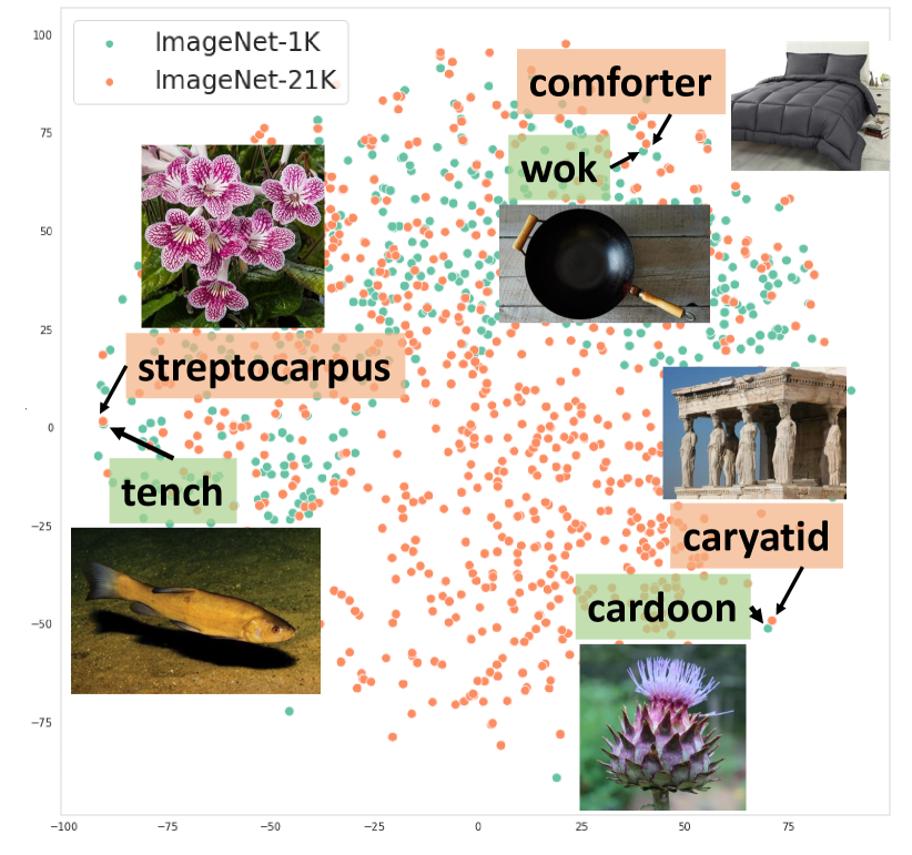
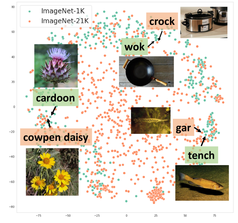
Figure 4: 2D $t$-SNE visualization of textual concepts encoded by the learned text encoder. We plot 1000 classes for both ImageNet-1K and ImageNet-21K. Given the category from ImageNet-1K (green box), we find the closest category from ImageNet-21K (orange box). Left: UniCL trained on ImageNet-1K; Right: UniCL trained on ImageNet-1K+GCC-15M. Better viewed in color.

For qualitative analysis, we visualize the 2D $t$-SNE [60] of the textual feature space in Fig. 4. Given a query concept from ImageNet-1K, we search the closest target concept from the remained 21K concepts in ImageNet-22K in the feature space. For better understanding, we also show the exemplar image corresponding to each concept. Clearly, model trained on ImageNet-1K can hardly generalize to understand the concepts from the other 21K concepts. In contrast, adding GCC-15M image-text pairs significantly improve the its understanding ability, as the retrieved target become more semantically similar to the queries in ImageNet-1K.

Training Data	Method	Metric
		Zero-shot		ImageNet-1K Finetuning	Linear Probe 18 datasets
		ImageNet-1K	14 datasets
YFCC-14M	CLIP	30.1	36.3	77.5	72.7
ImageNet-21K	UniCL	28.5	37.8	78.8	80.5
YFCC-14M + ImageNet-21K (half/half)	Multi-task	33.0	41.5	78.0	74.1
YFCC-14M + ImageNet-21K (half/half)	UniCL	36.4	45.5	79.0	80.0
YFCC-14M + ImageNet-21K	UniCL	40.5	49.1	80.2	81.6
ImageNet-22K	UniCL	66.8	38.9	80.3	82.0
YFCC-14M + ImageNet-22K	Multi-task	40.9	47.6	80.4	82.0
YFCC-14M + ImageNet-22K	UniCL	70.5	52.4	80.5	82.0
GCC-15M   + ImageNet-22K	Multi-task	50.6	51.8	79.9	82.5
GCC-15M   + ImageNet-22K	UniCL	71.3	53.8	80.0	82.1

Table 6: Ablation studies on the training datasets and tasks. Each model is pre-trained with 32 epochs following CLIP [48].

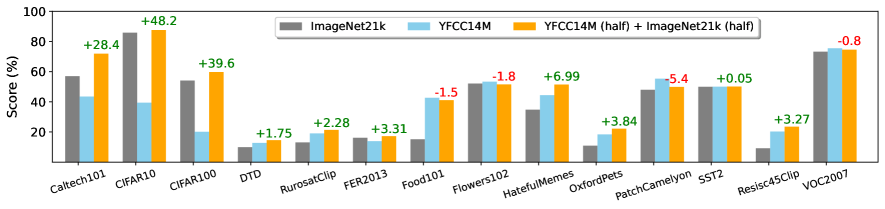
Figure 5: Zero-shot classification on 14 datasets. The gain between UniCL on mixed data and CLIP on YFCC-14M data is shown. UniCL combines the advantages of learning rich concept coverage from image-text pairs and discriminative representations from image-label data: UniCL outperforms both baselines significantly on the first 3 datasets, and shows higher averaged scores on others.

4.2.2 Benefit of image-label to image-text

We switch the role to study how image-label data can assist the learning with image-text pairs. Follow the protocols in CLIP [48], we use random crop as the data augmentation, a standard data sampler, and train all models for 32 epochs. We compare against two baselines: $(i)$ CLIP, a language-image contrastive learning method without label supervision, our UniCL can recover CLIP when merely using image-text pair for the training. $(ii)$ Multi-task learning that performs CE on image-label data, and CLIP on image-text data.

We report the results in Table 6. We first reproduced CLIP on YFCC-14M with Swin-Tiny. The ImageNet-1K zero-shot accuracy is 30.1%, which closely matches the reported number 31.2% with ResNet-50 in [48]. To ensure fair comparisons, we build a ImageNet-21K dataset by excluding the categories in ImageNet-1K from ImageNet-22K dataset, and train UniCL. Interestingly, it achieves comparable ImageNet-1K zero-shot performance to YFCC-14M. This indicates image-label data is arguably another good source of learning visual-semantic representations, which is nevertheless less studied in previous works. We combine half of ImageNet-21K and YFCC-14M datasets so that the total number of training instances remains the same, and train a UniCL model. This data unification boosts performance almost on all metrics, especially on zero-shot classification for ImageNet-1K (absolute $6\%>$ gain) and 14 datastes (absolute $7\%>$ gain). The detailed comparison on 14 datasets in Fig. 5, shows that UniCL wins on 11 out of 14 datasets. Besides zero-shot, our UniCL also achieves significant improvement (+7.3%) on linear probe compared with the CLIP baseline. With the full set of both datasets (row 4), the performance can be uniformly improved further.

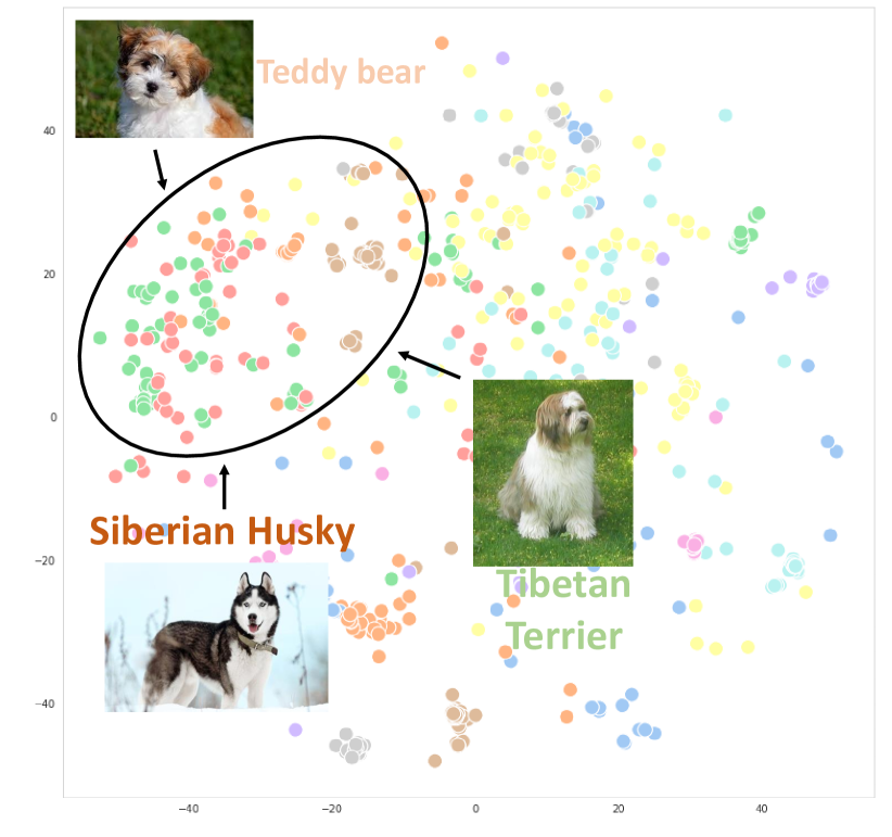
Figure 6: 2D $t$-SNE visualization of visual features from visual encoders. We randomly select images from 20 classes of ImageNet-1K and visualize the distribution for Left: CLIP trained on YFCC-14M; Right: UniCL trained on YFCC-14M (half)+ImageNet-21K (half). Three categories “teddy bear”,“siberian husky” and “tibetan terrier” are highlighted. Better viewed in color.

We compare our method with multi-task learner with different datasets. First, when using half of YFCC-14M and ImageNet-21K, our UniCL outperforms multi-task learner by a large margin across all tasks. When trained with the ImageNet-22K, the gaps shrink for ImageNet-1K finetuning and linear probe but remain for zero-shot recognition. This is mainly because ImageNet-22K cover all ImageNet-1K concepts and a large portion of categories in the linear probe datasets. Admittedly, Multi-task learner is a good representation learning method. However, because it isolates image-label and image-text pairs, it cannot learn a discriminative and semantic-rich feature space as our method.

Finally, to qualitatively show that how UniCL trained with image-label data yields a more discriminative feature space, we visualize the 2D $t$-SNE for the visual features of ImageNet-1K dataset in Fig. 6. Dogs with fine-grained breeds are heavily mixed together for the model trained on image-text pairs only. However, they are clearly grouped with the aid of image-label data from ImageNet-21K, even though it contains none of those dog breed concepts.

5 Conclusion

We have presented UniCL, a new contrastive learning paradigm for generic multi-modal representation learning. It is built in the image-text-label space, and empowered by our unified contrastive learning method. Such a unified paradigm prompts a seamless synergy between image-label and image-text pairs for discriminative and semantic-rich representation learning, which brings universal improvements on zero-shot, linear probe, finetuning benchmarks. Moreover, we discuss its connections to existing learning methods, and empirically demonstrated that our learning method stand-alone is a good alternative learner on pure image-label data.

Discussions. During our submission, we mainly focused on vision tasks such as image recognition and object detection, and based our model on public datasets. However, we refer the readers to Florence [72] for large-scale pretraining and evaluation on a boarder set of tasks including VQA and video understanding. We note that Florence used a huge amount of private data and thus recommend the suite of experiments in this paper as a baseline for future academic research.

Dataset	#Concepts	Vocab. Size	Train size	Test size	Evaluation metric	Source link	Linear Probe	Zero-shot
Food-101	102	139	75,750	25,250	Accuracy	Tensorflow	✓	✓
CIFAR-10	10	10	50,000	10,000	Accuracy	TensorFlow	✓	✓
CIFAR-100	100	100	50,000	10,000	Accuracy	TensorFlow	✓	✓
SUN397	397	432	19,850	19,850	Accuracy	Tensorflow	✓
Stanford Cars	196	291	8,144	8,041	Accuracy	Stanfold Cars	✓
FGVC Aircraft (variants)	100	115	6,667	3,333	Mean-per-class	FGVC website	✓
VOC2007 classification	20	20	5,011	4,952	11-point mAP	voc2007	✓	✓
Describable Textures	47	47	3,760	1,880	Accuracy	TensorFlow	✓	✓
Oxford-IIIT Pets	37	53	3,680	3,669	Mean-per-class	Oxford-IIIT Pet	✓	✓
Caltech-101	102	122	3,060	6084	Mean-per-class	TensorFlow	✓	✓
Oxford Flowers 102	102	147	2,040	6,149	Mean-per-class	TensorFlow	✓	✓
MNIST	10	10	60,000	10,000	Accuracy	TensorFlow	✓
FER 2013 ∗	8	12	32,298	3,589	Accuracy	Kaggle fer2013	✓	✓
STL10	10	10	5,000	8,000	Accuracy	TensorFlow	✓
GTSRB ∗	43	85	26,728	12,630	Accuracy	GTSRB website	✓
PatchCamelyon	2	6	294,912	32,768	Accuracy	TensorFlow	✓	✓
UCF101 ∗	101	153	9,537	3783	Accuracy	TensorFlow	✓
Hateful Memes	2	2	8,500	500	ROC-AUC	FaceBook	✓	✓
EuroSAT	10	20	5,000	5,000	Accuracy	TensorFlow		✓
Resisc45	45	59	3,150	25,200	Accuracy	TensorFlow		✓
Rendered-SST2	2	2	6,920	1,821	Accuracy	OpenAI		✓

Table 7: Statistics of datasets used in zero-shot and linear probe. ^∗ indicates dataset whose train/test size we obtained is slightly different from Table 9 in [48]. ✓indicates the dataset is used in this setting. The datasets are chosen based on the criterion if we can reproduce the numbers reported from [48] and their availability.

Appendix A Validation dataset details

In addition to the training datasets listed in our main submission, we list in Table 7 the statistics for all the validation datasets used in our experiments. Similar to the Table 1 in our main submission, we calculate the vocabulary size for each dataset, which is typically more than the number of concepts (classes).

Appendix B Experiment details

B.1 Training on image classification data

This part mainly explains the detailed experiment setups for Sec. 4.1 in our main submission.

Model architecture. We employ two representative architectures, ResNet [23] and Swin Transformer [44] to build the visual encoder. The globally pooled feature from last visual encoder layer is used as the visual feature. For language encoder, we use a 12-layer Transformer [61] with hidden dimension of 512 following [48]. Features from visual and textual encoder are projected to the same dimension of 512, using two linear projection layers.

Training protocol. For optimization, we use SGD [49] for all CNN models, while AdamW [32] for all models with Transformers on either vision or language side. We set the learning rate to 0.4 and 0.002, weight decay to 1e-4 and 0.05 for SGD and AdamW optimizer, respectively. All models are trained for 500 epochs with a batch size of 4096. We use same set of data augmentation and regularization as in [44], but do not use MixUp [75] and CutMix [73] except for the last column in Table 2 of our main submission. For all training, we used a cosine learning rate schedule, with 5 epochs and 20 epochs warmup for ResNet and Swin Transformer, respectively.

B.2 Training on image-text-label space

Training protocol for Sec. 4.2.1. We use Swin-Tiny as the visual encoder and follow the training settings in Section 4.1 mostly to train the models on the joint of image-label and image-text pairs. However, we notice there is a severe imbalance between image-label and image-text data as shown in Table 1 in our main submission (e.g., there are around 1.3M images in ImageNet-1K while above 12M images in GCC-12M dataset). To ensure that the model training is not biased to the dominant image-text pairs, we develop a balanced data sampler for two data types. More specifically, at each epoch, we randomly sample a subset of image-text pairs that has the equal or similar size to that of image-label data. In this case, the model sees half image-label data and half image-text data at each iteration for a balanced learning. We keep the number of training epochs the same as 500, so the effective number of training epochs on the image-text dataset is roughly 500$\times$(size of image-label dataset)/(size of image-text pair dataset). For example, the model learns from GCC-12M for around 40 epochs. We find this balanced sampling strategy is very important to achieve the reported performance in our main submission.

Training protocol for Sec. 4.2.2. We followed the training protocol in CLIP [48] for fair comparison. Specifically, we merely used random crop for dataset augmentation in all model trainings. All models including the baseline models are trained for 32 epochs, with batch size 4096, initial learning rate 1e-3 and weight decay 0.1. We also used a cosine learning rate scheduler with 5000 warmup iterations.

Appendix C More results

C.1 Results over separate datasets

In Figure 7, we show the zero-shot classification on 14 datasets by adding different image-caption pairs into the ImageNet-1K, i.e. the methods compared in Table 5 in the main text. UniCL takes the advantages of learning rich concept coverage from image-text pairs: On most of the datasets, it outperforms the baseline, especially on fine-grained classification tasks such as Food101 and OxfordPets.

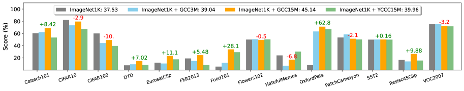
Figure 7: Zero-shot classification on 14 datasets by adding different image-caption pairs into the ImageNet-1K. The averaged scores of each method is reported in the legend. The gain of UniCL on mixed data (ImageNet1K+GCC15M) over image-label data (ImageNet1K) is shown.

C.2 Results with larger vision backbone

In our main submission, we used Swin-Tiny as the visual backbone to study how our UniCL perform when trained on the combination of image-label data ImageNet-21K and image-text pairs YFCC-14M in Table 6. Here, we investigate whether increase the capacity of the vision backbone can further improve the representation learning.

As shown in Table 8, we observe consistent trend as in Table 6 of our main submission. Though using similar amount of image-text-label corpus, combining two type of data can significantly improve the zero-shot recognition performance on both ImageNet-1K (8.6 points) and other 14 datasets in average (11.0 points). When using the full set of ImageNet-21K and YFCC-14M, both performance can be further improved significantly. These results suggest that our method is agnostic to different model sizes and thus a generic learning paradigm for visual-semantic representations. For comparison, we also list the numbers for Swin-Tiny models after each “/”. Clearly, increasing the visual encoder size brings substantial gains in all cases, and particularly significant for the combination of both data types.

Training Data	Method	Zero-shot
		ImageNet-1K	14 datasets
YFCC-14M	CLIP	32.4/30.1	37.5/36.3
ImageNet-21K	UniCL	29.9/28.5	42.4/37.8
YFCC-14M(half)+ImageNet-21K(half)	UniCL	41.0/36.4	48.5/45.5
YFCC-14M+ImageNet-21K	UniCL	43.8/40.5	52.2/49.1

Table 8: Ablation studies on the training datasets and tasks. We use Swin-Base [44] as the vision backbone. Each model is pre-trained with 32 epochs following CLIP [48]. Numbers before and after each “/” are with Swin-Base and Swin-Tiny, respectively.

C.3 Transfer to object detection

In the Table 5 of our main submission, we mainly studied whether image-text pairs can bring benefits to object detection transfer learning compared with the models solely trained on image-label data. As we demonstrated in Table 6 of our main submission, image-label data can help to learn more discriminative representations, and thus benefits ImageNet-1K finetuning and linear probing. Here, we further study whether the learned representations can generalize to object detection task as well. Specifically, we use the Swin-Tiny models pretrained in Table 6 as the vision backbones and train a Mask R-CNN model with 1$\times$ schedule following the default settings in Swin Transformer [44] based on Detectron2 [68]. In Table 9, we can see combining two data types with similar amount clearly improve the object detection performance by around 2 points for both box and mask mAP, compared with the CLIP-based model trained on YFCC-14M. This further validates our note that representations learned from pure image-text pair data usually lack the discirminative ability required by transfer learning to image recognition and object detection. As expected, using the full set (last row) brings further around 1 point improvement for both metrics. Along with the reported numbers in Table 5 of our main submission, these results together imply that adding image-text pairs to image-label data and the other way around can universally help to learn a better visual representations compared with the individual counterparts. Adding image-text pairs data can enrich and smoothen the semantic space which may implicitly prompt distinctive representations for the concepts in COCO object detection, while adding image-label data directly imposes the pressure to learn more discriminative representations.

Training Data	Method	Object Detection
		box mAP	mask mAP
YFCC-14M	CLIP	39.9	37.3
ImageNet-21K	UniCL	41.4	38.6
YFCC-14M(half)+ImageNet-21K(half)	UniCL	41.9	39.0
YFCC-14M+ImageNet-21K	UniCL	43.1	40.0

Table 9: Object detection transfer learning with different models. We use the pretrained Swin-Tiny models listed in Table 6 of our main submission as the vision backbone.

Appendix D More analysis

D.1 Concept distribution

The concepts residing in the training data is arguably crucial to the model learning. Both CLIP [48] and ALIGN [29] exhaustively collect hundreds of millions of image-text pairs to cover as many visual concepts as possible. Though the datasets used in our experiments are at much smaller scale, we are still interested in the concept distributions of different datasets. In Fig. 8, we show the occurrences of top 1000 concepts in GCC-3M, GCC-12M and YFCC-14M. Along with the remaining concepts that do not show here, all three datasets have extreme long-tail distributions. For example, the most frequent concept “view” in GCC-12M appears over 185,363 times, while the 10k-th concept “candle holder” only appears 501 times, knowing that there are more than 584k concepts in the whole set.

Interestingly, we find the overlap of most common concepts across three datasets is lower than what we expect. Table 10 shows the overlap ratios of top 10k concepts among three datasets. These relatively lower overlapping indicates the sufficient diversities and complementary among them.

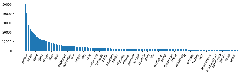
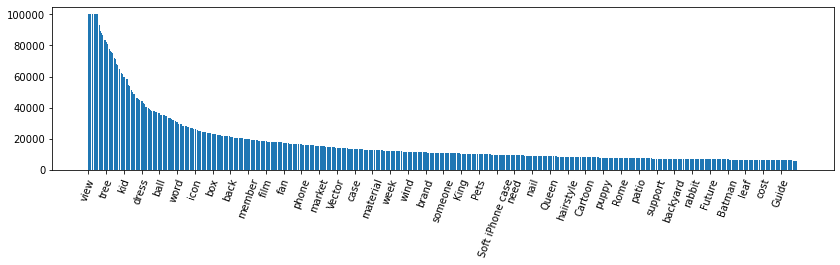
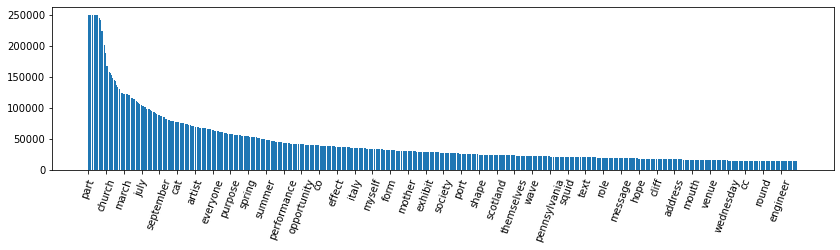
Figure 8: From top to bottom, bar charts are top 1000 most frequent concepts in GCC-3M, GCC-12M and YFCC-14M, respectively. We trim the heights of most frequent concepts for better display. For clarity, we display the concept name for every 25 concepts.

Dataset	GCC-3M	GCC-12M	YFCC-14M
GCC-3M	100%	46.5%	50.2%
GCC-12M	46.5%	100%	37.9%
YFCC-14M	50.2%	37.9%	100%

Table 10: Overlap ratio of top 10k concepts among GCC-3M, GCC-12M and YFCC-14M. The matrix is symmetric.

D.2 Concept coverage

Given the concept distributions above, we further investigate the concept coverage between training datasets and validation datasets. In Table 11, we calculate the coverage ratio to be the percentage of concepts mentioned by the pretraining data, including ImageNet-1K, ImageNet-21K, GCC-3M, GCC-12M and YFCC-14M. Coverage ratios equal or larger than 50% are highlighted.

Accordingly, for image-label dataset ImageNet-1K, it has some overlaps with CIFAR-100 (24.0%) and Caltech-101 (24.5%). This may explain why the zero-shot performance on these two datasets shown in Fig. 7 is relative higher. In contrast, we also notice that even with less or no coverage, the model pretrained on ImageNet-1K with our method still attain reasonably good zero-shot performance on datasets like CIFAR-10, Flowers102, Oxford Pet, etc.

Similarly, for ImageNet-21K, it covers a certain proportion of concepts in the validation sets, such as CIFAR-10, CIFAR-100, Caltech-101, etc, and we did observe high zero-shot recognition performance on them in the Table 6 of our main submission. Nevertheless, for other datasets like Hateful Memes, PatchCamelyon, there are zero concept overlaps, while our model still realizes reasonable performance. This indicates that our model is not just memorizing the concepts appearing in the training datasets, but also learns to understand the underlying structures of different concepts, which has been also demonstrated in Fig. 5 of our main submission.

Finally, we find image-text pairs data have higher coverage of concepts than image-label datasets almost on all validation sets. Among the three image-text pair datasets, GCC-12M has relatively higher coverage than the other two datasets. This may also explain why we observe better performance in the comparisons shown in Table 5 of our main submission. However, we also notice that higher concept coverage does not necessarily means better zero-shot performance. For example, even though all of these three datasets have a fully coverage of concepts in CIFAR-10 and CIFAR-100, adding them into the pretraining hurts the performance as shown in Fig. 7. We suspect there might be some significant gaps in the image domain between the pretraining and validation datasets even though they share common semantic concepts. Moreover, images in image-text pairs usually contain multiple objects, the coverage of concepts does not necessarily means the model can learn to grounding the concepts to the specific image contents. How to better leverage the image-text pair data and build a more gounded visual understanding worth further studies.

Dataset			ImageNet-1K		ImageNet-21K		GCC-3M		GCC-12M		YFCC-14M
Name	#Concepts	Vocab. Size	Cover.	#Img/C.	Cover.	#Img/C.	Cover.	#Img/C.	Cover.	#Img/C.	Cover.	#Img/C.
ImageNet-1K	1,000	1,233	100%	1300	0%	0	45.3%	247.0	78.5%	851.1	69.3%	1930.8
Food-101	102	139	4.0%	1300.0	20.8%	650.0	21.8%	39.8	58.4%	250.8	67.3%	408.8
CIFAR-10	10	10	0.0%	0.0	90.0%	650.0	100.0%	6175.4	100.0%	19969.8	100.0%	32998.9
CIFAR-100	100	100	24.0%	1300.0	65.0%	650.0	95.0%	3928.4	99.0%	15628.5	99.0%	18303.2
SUN397	397	432	5.0%	1300.0	28.5%	650.0	48.1%	818.9	65.5%	2355.4	66.5%	7043.2
Stanford Cars	196	291	0.0%	0.0	0.0%	0.0	0.0%	0.0	0.0%	0.0	0.0%	0.0
FGVC Aircraft (variants)	100	115	0.0%	0.0	0.0%	0.0	0.0%	0.0	22.0%	4.1	0.0%	0.0
VOC2007 classification	20	20	0.0%	0.0	75.0%	650.0	85.0%	14721.6	85.0%	19934.8	85.0%	31448.8
Describable Textures	47	47	0.0%	0.0	4.3%	650.0	14.9%	8.9	27.7%	53.2	36.2%	181.7
Oxford-IIIT Pets	37	53	5.4%	1300.0	13.5%	650.0	10.8%	80.9	64.9%	134.0	37.8%	169.0
Caltech-101	102	122	24.5%	1300.0	43.1%	650.0	66.6%	1633.8	83.3%	5249.7	87.3%	5017.7
Oxford Flowers 102	102	147	10.0%	1300.0	40.2%	650.0	17.6%	53.2	50.0%	194.3	65.7%	422.7
MNIST	10	10	0.0%	0.0	0.0%	0.0	40.0%	0.8	100.0%	46.0	90.0%	68.8
FER 2013 ∗	8	12	0.0%	0.0	8.3%	650.0	25.0%	5.9	41.7%	29.2	41.7%	11.5
STL10	10	10	0.0%	0.0	100%	650.0	100.0%	8778.6	100.0%	28547.6	100.0%	45587.5
GTSRB ∗	43	85	0.0%	0.0	0.0%	0.0	2.3%	12.7	2.3%	52.9	2.3%	551.3
PatchCamelyon	2	6	0.0%	0.0	0.0%	0.0	0.0%	0.0	50.0%	143.0	50.0%	15.0
UCF101 ∗	101	153	0.0%	0.0	0.0%	0.0	0.0%	0.0	51.5%	66.4	0.0%	0.0
Hateful Memes	2	2	0.0%	0.0	0.0%	0.0	50.0%	79.5	50.0%	2742.5	50.0%	321.5
EuroSAT	10	20	0.0%	0.0	0.0%	0.0	20.0%	2946.6	30.0%	5266.3	30.0%	15458.7
Resisc45	45	59	8.9%	1300.0	26.7%	650.0	71.1%	3688.6	75.6%	7572.0	80.0%	26317.6
Rendered-SST2	2	2	0.0%	0.0	50.0%	650.0	50.0%	1.0	100.0%	114.0	100.0%	1259.0

Table 11: Statistics of concept coverage between training and validation dataests. ^∗ indicates dataset whose train/test size we obtained is slightly different from Table 9 in [48]. “Cover.” denotes the coverage ratio of concepts in target dataset by the training dataet. For those with non-zero coverage ratio, we also list the average number of images for each concept. For ImageNet-1K and ImageNet-21K, we estimate the number of images per concept by dividing the total number of images by total number of concepts, which are 1300 and 650, respectively

D.3 Concept visualizations

In Fig. 9, we further show the concept embeddings for two models as in Fig. 4 in our main submission. Fig. 9 left shows the model trained only on ImageNet-1K while right shows the model trained jointly with ImageNet-1K and GCC-15M. The model trained with two type of data understand the novel concepts from ImageNet-21K much better than the left one. For example, the left model put “porthole” and porcupine close to each other but the former is a circular window and latter is an animal. In contrast, the model at right side can easily find the “porcuponefish” as the close neighbor. Similarly, the left model mix “goblet” and “coverlet”, probably because they share the same suffix. Our model on right side finds one of the most matched concepts “liqueur glass” which is semantically and visually similar to the query concept. Similar trend is also observed in Fig. 10. All these visualizations demonstrate that our model trained with both type of data has learned the visually-grounded semantic meanings for various concepts.

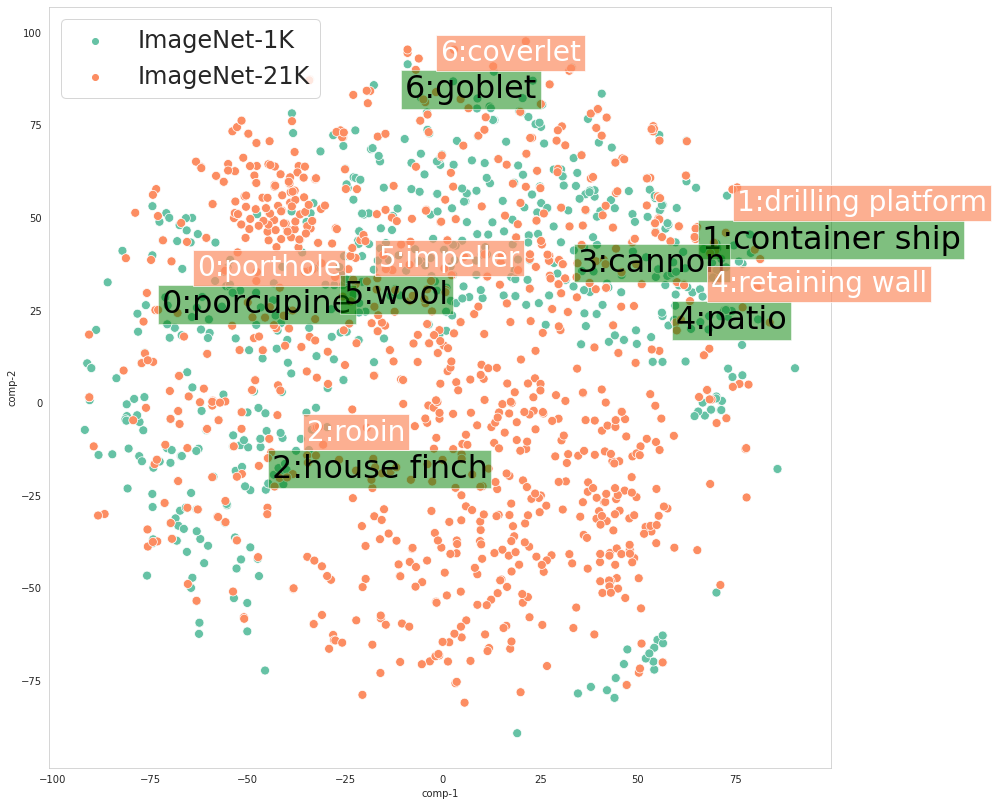
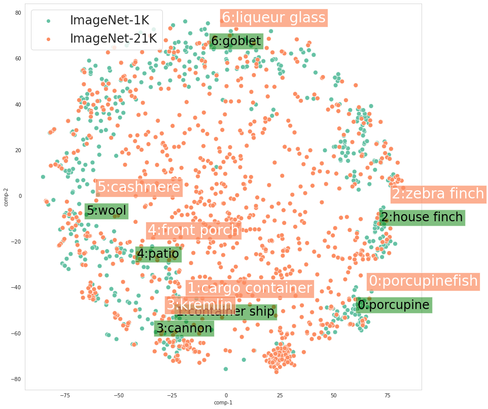
Figure 9: Similar to Fig. 4 in our main submission, we further visualize the t-SNE embedding for visual concepts with models trained with ImageNet-1K (left) and ImageNet-1K+GCC-15M (right).

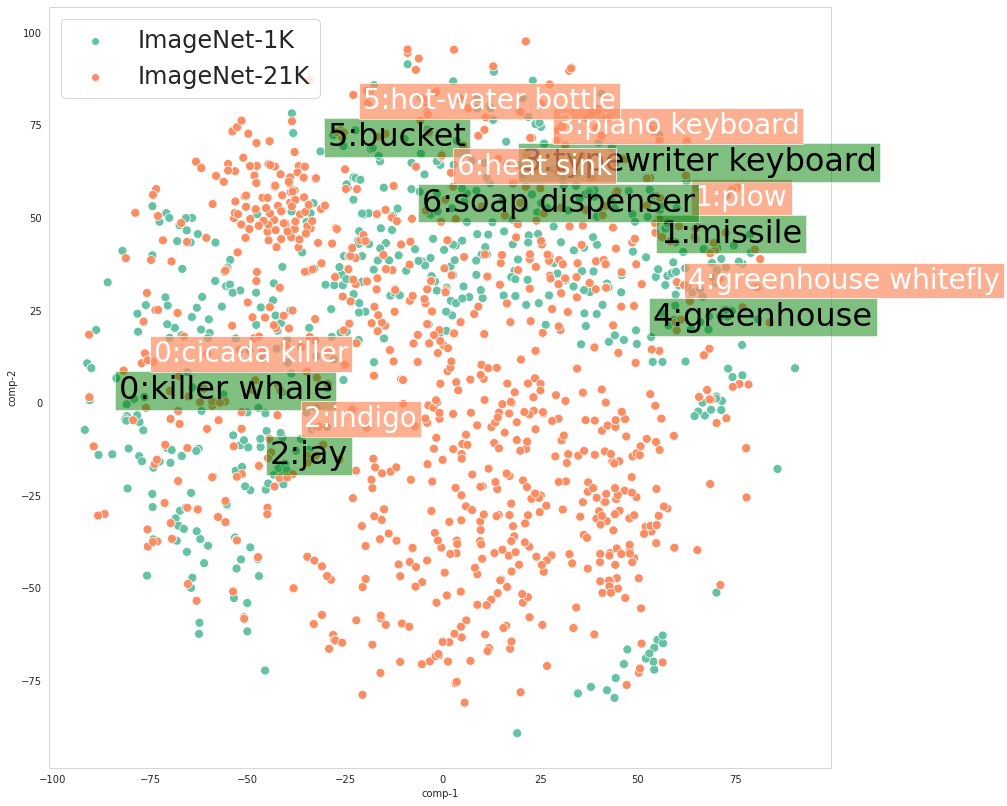
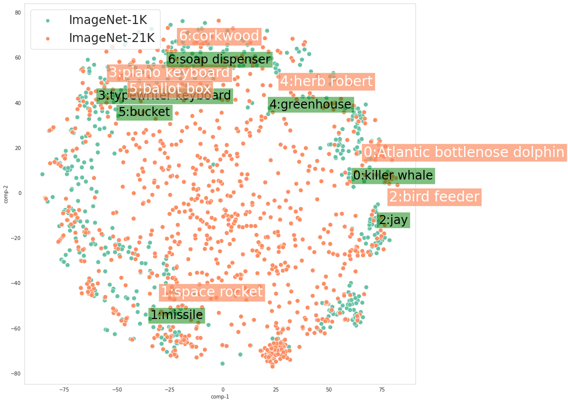
Figure 10: Similar to Fig. 9, we visualize the t-SNE embedding for another random set of visual concepts with models trained with ImageNet-1K (left) and ImageNet-1K+GCC-15M (right). Clearly, our model learned from the combination of image-label and image-text pairs can understand more number of visual concepts.

References

- [1] Harsh Agrawal, Karan Desai, Yufei Wang, Xinlei Chen, Rishabh Jain, Mark Johnson, Dhruv Batra, Devi Parikh, Stefan Lee, and Peter Anderson. nocaps: novel object captioning at scale. In Proceedings of the IEEE/CVF International Conference on Computer Vision, pages 8948–8957, 2019.
- [2] Stanislaw Antol, Aishwarya Agrawal, Jiasen Lu, Margaret Mitchell, Dhruv Batra, C Lawrence Zitnick, and Devi Parikh. Vqa: Visual question answering. In Proceedings of the IEEE international conference on computer vision, pages 2425–2433, 2015.
- [3] Mathilde Caron, Ishan Misra, Julien Mairal, Priya Goyal, Piotr Bojanowski, and Armand Joulin. Unsupervised learning of visual features by contrasting cluster assignments. arXiv preprint arXiv:2006.09882, 2020.
- [4] Mathilde Caron, Hugo Touvron, Ishan Misra, Hervé Jégou, Julien Mairal, Piotr Bojanowski, and Armand Joulin. Emerging properties in self-supervised vision transformers. ICCV, 2021.
- [5] Soravit Changpinyo, Piyush Sharma, Nan Ding, and Radu Soricut. Conceptual 12m: Pushing web-scale image-text pre-training to recognize long-tail visual concepts. In Proceedings of the IEEE/CVF Conference on Computer Vision and Pattern Recognition, pages 3558–3568, 2021.
- [6] Ting Chen, Simon Kornblith, Mohammad Norouzi, and Geoffrey Hinton. A simple framework for contrastive learning of visual representations. In International conference on machine learning, pages 1597–1607. PMLR, 2020.
- [7] Xinlei Chen and Kaiming He. Exploring simple siamese representation learning. In CVPR, 2021.
- [8] Xinlei Chen, Saining Xie, and Kaiming He. An empirical study of training self-supervised visual transformers. ICCV, 2021.
- [9] François Chollet. Information-theoretical label embeddings for large-scale image classification. arXiv preprint arXiv:1607.05691, 2016.
- [10] Jia Deng, Wei Dong, Richard Socher, Li-Jia Li, Kai Li, and Li Fei-Fei. Imagenet: A large-scale hierarchical image database. In 2009 IEEE conference on computer vision and pattern recognition, pages 248–255. Ieee, 2009.
- [11] Jiankang Deng, Yuxiang Zhou, and Stefanos Zafeiriou. Marginal loss for deep face recognition. In Proceedings of the IEEE Conference on Computer Vision and Pattern Recognition Workshops, pages 60–68, 2017.
- [12] Karan Desai and Justin Johnson. Virtex: Learning visual representations from textual annotations. In Proceedings of the IEEE/CVF Conference on Computer Vision and Pattern Recognition, pages 11162–11173, 2021.
- [13] Jacob Devlin, Ming-Wei Chang, Kenton Lee, and Kristina Toutanova. Bert: Pre-training of deep bidirectional transformers for language understanding. arXiv preprint arXiv:1810.04805, 2018.
- [14] Jeff Donahue, Yangqing Jia, Oriol Vinyals, Judy Hoffman, Ning Zhang, Eric Tzeng, and Trevor Darrell. Decaf: A deep convolutional activation feature for generic visual recognition. In International conference on machine learning, pages 647–655. PMLR, 2014.
- [15] Alexey Dosovitskiy, Lucas Beyer, Alexander Kolesnikov, Dirk Weissenborn, Xiaohua Zhai, Thomas Unterthiner, Mostafa Dehghani, Matthias Minderer, Georg Heigold, Sylvain Gelly, et al. An image is worth 16x16 words: Transformers for image recognition at scale. arXiv preprint arXiv:2010.11929, 2020.
- [16] Andrea Frome, Greg S Corrado, Jon Shlens, Samy Bengio, Jeff Dean, Marc’Aurelio Ranzato, and Tomas Mikolov. Devise: A deep visual-semantic embedding model. Advances in neural information processing systems, 26, 2013.
- [17] Albert Gordo and Diane Larlus. Beyond instance-level image retrieval: Leveraging captions to learn a global visual representation for semantic retrieval. In Proceedings of the IEEE conference on computer vision and pattern recognition, pages 6589–6598, 2017.
- [18] Priya Goyal, Mathilde Caron, Benjamin Lefaudeux, Min Xu, Pengchao Wang, Vivek Pai, Mannat Singh, Vitaliy Liptchinsky, Ishan Misra, Armand Joulin, et al. Self-supervised pretraining of visual features in the wild. arXiv preprint arXiv:2103.01988, 2021.
- [19] Priya Goyal, Dhruv Mahajan, Abhinav Gupta, and Ishan Misra. Scaling and benchmarking self-supervised visual representation learning. In ICCV, 2019.
- [20] Jean-Bastien Grill, Florian Strub, Florent Altché, Corentin Tallec, Pierre H Richemond, Elena Buchatskaya, Carl Doersch, Bernardo Avila Pires, Zhaohan Daniel Guo, Mohammad Gheshlaghi Azar, et al. Bootstrap your own latent: A new approach to self-supervised learning. NeurIPS, 2020.
- [21] Kaiming He, Haoqi Fan, Yuxin Wu, Saining Xie, and Ross Girshick. Momentum contrast for unsupervised visual representation learning. In CVPR, 2020.
- [22] Kaiming He, Georgia Gkioxari, Piotr Dollár, and Ross Girshick. Mask r-cnn. In Proceedings of the IEEE international conference on computer vision, pages 2961–2969, 2017.
- [23] Kaiming He, Xiangyu Zhang, Shaoqing Ren, and Jian Sun. Deep residual learning for image recognition. In Proceedings of the IEEE conference on computer vision and pattern recognition, pages 770–778, 2016.
- [24] Olivier J Hénaff, Aravind Srinivas, Jeffrey De Fauw, Ali Razavi, Carl Doersch, SM Eslami, and Aaron van den Oord. Data-efficient image recognition with contrastive predictive coding. arXiv preprint arXiv:1905.09272, 2019.
- [25] Matthew Honnibal and Ines Montani. spaCy 2: Natural language understanding with Bloom embeddings, convolutional neural networks and incremental parsing. To appear, 2017.
- [26] Jie Hu, Li Shen, and Gang Sun. Squeeze-and-excitation networks. In Proceedings of the IEEE conference on computer vision and pattern recognition, pages 7132–7141, 2018.
- [27] Drew A Hudson and Christopher D Manning. Gqa: A new dataset for real-world visual reasoning and compositional question answering. In Proceedings of the IEEE/CVF conference on computer vision and pattern recognition, pages 6700–6709, 2019.
- [28] Dinesh Jayaraman and Kristen Grauman. Zero shot recognition with unreliable attributes. arXiv preprint arXiv:1409.4327, 2014.
- [29] Chao Jia, Yinfei Yang, Ye Xia, Yi-Ting Chen, Zarana Parekh, Hieu Pham, Quoc V Le, Yunhsuan Sung, Zhen Li, and Tom Duerig. Scaling up visual and vision-language representation learning with noisy text supervision. arXiv preprint arXiv:2102.05918, 2021.
- [30] Prannay Khosla, Piotr Teterwak, Chen Wang, Aaron Sarna, Yonglong Tian, Phillip Isola, Aaron Maschinot, Ce Liu, and Dilip Krishnan. Supervised contrastive learning. arXiv preprint arXiv:2004.11362, 2020.
- [31] Wonjae Kim, Bokyung Son, and Ildoo Kim. Vilt: Vision-and-language transformer without convolution or region supervision. arXiv preprint arXiv:2102.03334, 2021.
- [32] Diederik P Kingma and Jimmy Ba. Adam: A method for stochastic optimization. arXiv preprint arXiv:1412.6980, 2014.
- [33] Alexander Kolesnikov, Lucas Beyer, Xiaohua Zhai, Joan Puigcerver, Jessica Yung, Sylvain Gelly, and Neil Houlsby. Big transfer (bit): General visual representation learning. In Computer Vision–ECCV 2020: 16th European Conference, Glasgow, UK, August 23–28, 2020, Proceedings, Part V 16, pages 491–507. Springer, 2020.
- [34] Alex Krizhevsky, Geoffrey Hinton, et al. Learning multiple layers of features from tiny images. 2009.
- [35] Alex Krizhevsky, Ilya Sutskever, and Geoffrey E Hinton. Imagenet classification with deep convolutional neural networks. Advances in neural information processing systems, 25:1097–1105, 2012.
- [36] Yann LeCun, Yoshua Bengio, et al. Convolutional networks for images, speech, and time series.
- [37] Yann LeCun, Bernhard Boser, John Denker, Donnie Henderson, Richard Howard, Wayne Hubbard, and Lawrence Jackel. Handwritten digit recognition with a back-propagation network. Advances in neural information processing systems, 2, 1989.
- [38] Chunyuan Li, Jianwei Yang, Pengchuan Zhang, Mei Gao, Bin Xiao, Xiyang Dai, Lu Yuan, and Jianfeng Gao. Efficient self-supervised vision transformers for representation learning. arXiv preprint arXiv:2106.09785, 2021.
- [39] Junnan Li, Ramprasaath R Selvaraju, Akhilesh Deepak Gotmare, Shafiq Joty, Caiming Xiong, and Steven Hoi. Align before fuse: Vision and language representation learning with momentum distillation. arXiv preprint arXiv:2107.07651, 2021.
- [40] Xiujun Li, Xi Yin, Chunyuan Li, Pengchuan Zhang, Xiaowei Hu, Lei Zhang, Lijuan Wang, Houdong Hu, Li Dong, Furu Wei, et al. Oscar: Object-semantics aligned pre-training for vision-language tasks. In European Conference on Computer Vision, pages 121–137. Springer, 2020.
- [41] Min Lin, Qiang Chen, and Shuicheng Yan. Network in network. arXiv preprint arXiv:1312.4400, 2013.
- [42] Tsung-Yi Lin, Michael Maire, Serge Belongie, James Hays, Pietro Perona, Deva Ramanan, Piotr Dollár, and C Lawrence Zitnick. Microsoft coco: Common objects in context. In European conference on computer vision, pages 740–755. Springer, 2014.
- [43] Weiyang Liu, Yandong Wen, Zhiding Yu, and Meng Yang. Large-margin softmax loss for convolutional neural networks. In ICML, volume 2, page 7, 2016.
- [44] Ze Liu, Yutong Lin, Yue Cao, Han Hu, Yixuan Wei, Zheng Zhang, Stephen Lin, and Baining Guo. Swin transformer: Hierarchical vision transformer using shifted windows. ICCV, 2021.
- [45] Jiasen Lu, Dhruv Batra, Devi Parikh, and Stefan Lee. Vilbert: Pretraining task-agnostic visiolinguistic representations for vision-and-language tasks. arXiv preprint arXiv:1908.02265, 2019.
- [46] Thomas Mensink, Efstratios Gavves, and Cees GM Snoek. Costa: Co-occurrence statistics for zero-shot classification. In Proceedings of the IEEE conference on computer vision and pattern recognition, pages 2441–2448, 2014.
- [47] Kevin P Murphy. Machine learning: a probabilistic perspective. MIT press, 2012.
- [48] Alec Radford, Jong Wook Kim, Chris Hallacy, Aditya Ramesh, Gabriel Goh, Sandhini Agarwal, Girish Sastry, Amanda Askell, Pamela Mishkin, Jack Clark, et al. Learning transferable visual models from natural language supervision. arXiv preprint arXiv:2103.00020, 2021.
- [49] David E Rumelhart, Geoffrey E Hinton, and Ronald J Williams. Learning representations by back-propagating errors. nature, 323(6088):533–536, 1986.
- [50] Mert Bulent Sariyildiz, Julien Perez, and Diane Larlus. Learning visual representations with caption annotations. In European Conference on Computer Vision, pages 153–170. Springer, 2020.
- [51] Piyush Sharma, Nan Ding, Sebastian Goodman, and Radu Soricut. Conceptual captions: A cleaned, hypernymed, image alt-text dataset for automatic image captioning. In Proceedings of the 56th Annual Meeting of the Association for Computational Linguistics (Volume 1: Long Papers), pages 2556–2565, 2018.
- [52] Kihyuk Sohn. Improved deep metric learning with multi-class n-pair loss objective. In Advances in neural information processing systems, pages 1857–1865, 2016.
- [53] Weijie Su, Xizhou Zhu, Yue Cao, Bin Li, Lewei Lu, Furu Wei, and Jifeng Dai. Vl-bert: Pre-training of generic visual-linguistic representations. arXiv preprint arXiv:1908.08530, 2019.
- [54] Christian Szegedy, Wei Liu, Yangqing Jia, Pierre Sermanet, Scott Reed, Dragomir Anguelov, Dumitru Erhan, Vincent Vanhoucke, and Andrew Rabinovich. Going deeper with convolutions. In Proceedings of the IEEE conference on computer vision and pattern recognition, pages 1–9, 2015.
- [55] Christian Szegedy, Vincent Vanhoucke, Sergey Ioffe, Jon Shlens, and Zbigniew Wojna. Rethinking the inception architecture for computer vision. In Proceedings of the IEEE conference on computer vision and pattern recognition, pages 2818–2826, 2016.
- [56] Bart Thomee, David A Shamma, Gerald Friedland, Benjamin Elizalde, Karl Ni, Douglas Poland, Damian Borth, and Li-Jia Li. Yfcc100m: The new data in multimedia research. Communications of the ACM, 59(2):64–73, 2016.
- [57] Yonglong Tian, Dilip Krishnan, and Phillip Isola. Contrastive multiview coding. arXiv preprint arXiv:1906.05849, 2019.
- [58] Yonglong Tian, Chen Sun, Ben Poole, Dilip Krishnan, Cordelia Schmid, and Phillip Isola. What makes for good views for contrastive learning. arXiv preprint arXiv:2005.10243, 2020.
- [59] Hugo Touvron, Matthieu Cord, Matthijs Douze, Francisco Massa, Alexandre Sablayrolles, and Hervé Jégou. Training data-efficient image transformers & distillation through attention. In International Conference on Machine Learning, pages 10347–10357. PMLR, 2021.
- [60] Laurens Van der Maaten and Geoffrey Hinton. Visualizing data using t-sne. Journal of machine learning research, 2008.
- [61] Ashish Vaswani, Noam Shazeer, Niki Parmar, Jakob Uszkoreit, Llion Jones, Aidan N Gomez, Łukasz Kaiser, and Illia Polosukhin. Attention is all you need. In Advances in neural information processing systems, pages 5998–6008, 2017.
- [62] Liwei Wang, Yin Li, Jing Huang, and Svetlana Lazebnik. Learning two-branch neural networks for image-text matching tasks. IEEE Transactions on Pattern Analysis and Machine Intelligence, 41(2):394–407, 2018.
- [63] Liwei Wang, Yin Li, and Svetlana Lazebnik. Learning deep structure-preserving image-text embeddings. In Proceedings of the IEEE conference on computer vision and pattern recognition, pages 5005–5013, 2016.
- [64] Wenhai Wang, Enze Xie, Xiang Li, Deng-Ping Fan, Kaitao Song, Ding Liang, Tong Lu, Ping Luo, and Ling Shao. Pyramid vision transformer: A versatile backbone for dense prediction without convolutions. arXiv preprint arXiv:2102.12122, 2021.
- [65] Xiaolong Wang, Yufei Ye, and Abhinav Gupta. Zero-shot recognition via semantic embeddings and knowledge graphs. In Proceedings of the IEEE conference on computer vision and pattern recognition, pages 6857–6866, 2018.
- [66] Zirui Wang, Jiahui Yu, Adams Wei Yu, Zihang Dai, Yulia Tsvetkov, and Yuan Cao. Simvlm: Simple visual language model pretraining with weak supervision. arXiv preprint arXiv:2108.10904, 2021.
- [67] Haiping Wu, Bin Xiao, Noel Codella, Mengchen Liu, Xiyang Dai, Lu Yuan, and Lei Zhang. Cvt: Introducing convolutions to vision transformers. arXiv preprint arXiv:2103.15808, 2021.
- [68] Yuxin Wu, Alexander Kirillov, Francisco Massa, Wan-Yen Lo, and Ross Girshick. Detectron2. https://github.com/facebookresearch/detectron2, 2019.
- [69] Yongqin Xian, Zeynep Akata, Gaurav Sharma, Quynh Nguyen, Matthias Hein, and Bernt Schiele. Latent embeddings for zero-shot classification. In Proceedings of the IEEE conference on computer vision and pattern recognition, pages 69–77, 2016.
- [70] Yongqin Xian, Bernt Schiele, and Zeynep Akata. Zero-shot learning-the good, the bad and the ugly. In Proceedings of the IEEE Conference on Computer Vision and Pattern Recognition, pages 4582–4591, 2017.
- [71] Jianwei Yang, Chunyuan Li, Pengchuan Zhang, Xiyang Dai, Bin Xiao, Lu Yuan, and Jianfeng Gao. Focal attention for long-range interactions in vision transformers. Advances in Neural Information Processing Systems, 34, 2021.
- [72] Lu Yuan, Dongdong Chen, Yi-Ling Chen, Noel Codella, Xiyang Dai, Jianfeng Gao, Houdong Hu, Xuedong Huang, Boxin Li, Chunyuan Li, et al. Florence: A new foundation model for computer vision. arXiv preprint arXiv:2111.11432, 2021.
- [73] Sangdoo Yun, Dongyoon Han, Seong Joon Oh, Sanghyuk Chun, Junsuk Choe, and Youngjoon Yoo. Cutmix: Regularization strategy to train strong classifiers with localizable features. In Proceedings of the IEEE/CVF International Conference on Computer Vision, pages 6023–6032, 2019.
- [74] Rowan Zellers, Yonatan Bisk, Ali Farhadi, and Yejin Choi. From recognition to cognition: Visual commonsense reasoning. In Proceedings of the IEEE/CVF Conference on Computer Vision and Pattern Recognition, pages 6720–6731, 2019.
- [75] Hongyi Zhang, Moustapha Cisse, Yann N Dauphin, and David Lopez-Paz. mixup: Beyond empirical risk minimization. arXiv preprint arXiv:1710.09412, 2017.
- [76] Pengchuan Zhang, Xiyang Dai, Jianwei Yang, Bin Xiao, Lu Yuan, Lei Zhang, and Jianfeng Gao. Multi-scale vision longformer: A new vision transformer for high-resolution image encoding. In Proceedings of the IEEE/CVF International Conference on Computer Vision, pages 2998–3008, 2021.
- [77] Pengchuan Zhang, Xiujun Li, Xiaowei Hu, Jianwei Yang, Lei Zhang, Lijuan Wang, Yejin Choi, and Jianfeng Gao. Vinvl: Revisiting visual representations in vision-language models. In Proceedings of the IEEE/CVF Conference on Computer Vision and Pattern Recognition, pages 5579–5588, 2021.
- [78] Yuhao Zhang, Hang Jiang, Yasuhide Miura, Christopher D Manning, and Curtis P Langlotz. Contrastive learning of medical visual representations from paired images and text. arXiv preprint arXiv:2010.00747, 2020.