Collecting, Classifying, Analyzing, and Using Real-World Elections

Abstract

We present a collection of $7582$ real-world elections divided into $25$ datasets from various sources ranging from sports competitions over music charts to survey- and indicator-based rankings. We provide evidence that the collected elections complement already publicly available data from the PrefLib database, which is currently the biggest and most prominent source containing $701$ real-world elections from $36$ datasets [53]. Using the map of elections framework [76], we divide the datasets into three categories and conduct an analysis of the nature of our elections. To evaluate the practical applicability of previous theoretical research on (parameterized) algorithms and to gain further insights into the collected elections, we analyze different structural properties of our elections including the level of agreement between voters and election’s distances from restricted domains such as single-peakedness. Lastly, we use our diverse set of collected elections to shed some further light on several traditional questions from social choice, for instance, on the number of occurrences of the Condorcet paradox and on the consensus among different voting rules.

1 Introduction

The area of computational social choice is concerned with the algorithmic and axiomatic analysis of collective decision-making problems, where given a set of agents with preferences over some alternatives the task is to select a “compromise” alternative [12]. One important part of computational social choice is the study of algorithmic aspects of election-related problems such as the computation and manipulation of voting rules [86, 48, 33, 21, 17]. While in the early years of the field the main focus lay on the study of the theoretical worst-case computational complexity of these problems, in recent years the focus has at least partially shifted towards the practical applicability of theoretical research (see e.g., [37, 81, 46, 76, 41, 8]). Two classical social choice questions which have been extensively studied from an empirical perspective are the number of occurrences of voting paradoxes [18, 39, 13, 63] and the consensus among voting rules [18, 39, 66, 67, 52, 23, 64]. Nevertheless, there are still many subareas that lack empirical research. For instance, there are numerous theoretical papers designing parameterized algorithms for elections that are close to being single-peaked (see e.g. [85, 84, 22, 83, 35, 56, 73]). To the best of our knowledge, only Sui et al. [75] measured the distance of real-world elections from being single-peaked and detected that most elections are far away. Thus, the practical applicability of the developed algorithms is largely unclear.

Given that some collective decision-making problems can have a crucial impact on people’s lives, the general rarity of experimental works can be seen as slightly worrisome. While papers proposing a collective decision-making mechanism often conduct an analysis of the mechanism’s axiomatic and computational properties, a rigorous testing on real-world data is often missing. However, such an analysis would be highly beneficial, as axiomatic and computational complexity guarantees are often outperformed in practice [1, 79, 20, 78, 36, 72, 15]. Being able to conduct meaningful tests is thus crucial to better understand the practical aspects of collective decision-making mechanisms and to ultimately select the one that behaves “fairest” in practice.

One reason for the general rarity of experimental works in voting validating the applicability of theoretical research might be the lack of data. To tackle this issue, in 2013, Mattei and Walsh [54, 53] started the very useful PrefLib platform, a database for real-world election data. Many community members have contributed to this popular platform over the past years and at the moment it contains $701$ real-world elections dived into $36$ datasets (see Boehmer et al. [10, Table 5] for a recent overview of the datasets). Many elections from PrefLib are based on humans expressing opinions over alternatives, e.g., over candidates in an election, over movies, or types of sushi. However, due to this nature of these elections, most of them either have few candidates or voters express only partial preferences which can include many ties. In fact, as observed by Boehmer et al. [10, Table 5], there are only $165$ elections from $8$ sources on PrefLib with $10$ or more candidates where votes include not too many ties. The goal of this paper is to contribute to the rise of experimental works in computational social choice by executing the following four steps:

Step 1: Collecting Data.

In Section 3, we present our collection of $7582$ real-world elections divided into $25$ datasets. We preprocess the data by deleting candidates and voters until each voter ranks all candidates. Subsequently, to be able to better compare the properties of our elections, for each dataset we create $500$ elections containing $30$ voters over $15$ candidates. Our real-world elections differ from most of the already publicly available ones in three aspects: First, they contain virtually no ties and are of various sizes (the average number of candidates varies from around $20$ to above $800$, while the average number of voters ranges from around $12$ to over $1400$). Moreover, even after deleting voters and candidates until all voters rank all candidates, most elections are still of at least medium size. As a majority of algorithms are designed for such so-called complete elections, this is a very important step to ensure the usefulness of our data for experimental works. In the past, elections have been often completed by appending missing candidates in random order or based on the preference of other voters [24, 10]. Our approach offers the clear advantage that preferences in the final election are not distorted in any way: Each pairwise ordering of a voter represents its true opinion. Second, unlike a majority of elections on PrefLib, our datasets are not based on humans explicitly expressing preferences over alternatives. Admittedly, this might be considered as a drawback of our data as political elections are still often thought of as the prime application of social choice theory. Nevertheless, we want to remark that voting is also relevant and already used in many other contexts, e.g., in multi-agent systems, or in sports, when aggregating the results of multiple competitions into a final ranking. Third, around half of our datasets arise from time-based preferences, i.e., capture in one form or another the changing preferences of agents over time. Time-based elections might not directly match ones intuition for an election; however, preferences obtained at different points in time are also frequently collected in an election (for instance, when deciding on the overall winner of multiple competitions). Notably, while there are already some theoretical works dealing with such time-evolving preferences [7, 47, 62, 16], as pointed out by Mattei and Walsh [54], there are only very few such elections currently publicly available.

Step 2: Classifying Data.

In Section 4, we apply the map of elections framework of Szufa et al. [76] and Boehmer et al. [9] to visualize the collected elections as points on a map. Using this, we detect that one of our datasets seems to fall into a so-far vacant part of the “space of elections”. Moreover, based on their positions on the map, we propose a classification of our datasets into three categories and observe in the subsequent experiments that datasets from one category typically have similar properties. This suggests that if one wants to run experiments on our data, it should be sufficient to use few datasets from each of the three categories.

Step 3: Analyzing Data.

In Sections 5 and 6, we analyze various structural properties of the collected elections. This analysis serves three purposes: First, we aim for a better understanding of the collected elections. Second, we want to gain some insights into the relationship between the different properties. Third, we try to contribute to putting the research on parameterized algorithms for voting-related problems on an empirical basis by measuring already used parameters. Unfortunately, we find that most of them are typically quite large and thus that most algorithms developed for these parameters are probably not really practically usable on our data. Briefly put, in Section 5 we analyze the degree of similarity between voters in an election, while in Section 6 we check which of our elections are (close to) a restricted domain.

Step 4: Using Data.

In Section 7, we use our collected elections to address some classical and already empirically researched questions from social choice, such as the frequency of Condorcet winners and the consensus among voting rules. While we partly confirm previous findings, for instance, that most elections have a Condorcet winner and that voting rules often return the same winner, we find contradicting evidence for others and also identify some datasets showing a distinct behavior. This indicates that our datasets are quite different from each other with some of them showing rarely observable and non-standard behavior, making them collectively well-suited for experimental research.

Our original and preprocessed election data is available at github.com/n-boehmer/Collecting-Classifying-Analyzing-and-Using-Real-World-Elections. Most (sub)sections start with a list of main take-away messages summarizing the contribution of this (sub)section.

2 Preliminaries

For a set $S$ and an integer $k\in\mathbb{N}$, we denote as ${{S}\choose{k}}$ the set of all $k$-element subsets of $S$.

Preference Orders. For a set $C$ of candidates, let $\mathcal{L}(C)$ denote the set of all total orders over $C$. We refer to the elements of $\mathcal{L}(C)$ as preference orders, votes, or voters.

Elections. An election $E$ is defined by a set of $C=\{c_{1},\dots,c_{m}\}$ of $m$ candidates and a collection $V=(v_{1},\dots,v_{n})$ of $n$ voters with $v_{i}\in\mathcal{L}(C)$ for each $i\in[n]$. For a voter $v\in V$ and two candidates $a,b\in C$, we write $a\succ_{v}b$ to denote that $v$ prefers $a$ to $b$. We say that voter $v\in V$ ranks candidate $c\in C$ in position $i\in[m]$ if $v$ prefers exactly $i-1$ candidates from $C\setminus\{c\}$ to $c$. We refer to the candidate which a voter ranks in the first position as its top-choice.

Kendall Tau Distance. For two votes $v,v^{\prime}\in\mathcal{L}(C)$, their Kendall tau distance ${\mathrm{KT}}(v,v^{\prime})$ is defined as the number of candidate pairs on which orderings $v$ and $v^{\prime}$ disagree: $|\{c,c^{\prime}\in{{C}\choose{2}}\mid(c\succ_{v}c^{\prime}\wedge c^{\prime}\succ_{v^{\prime}}c)\vee(c\succ_{v^{\prime}}c^{\prime}\wedge c^{\prime}\succ_{v}c)\}|$. Alternatively, ${\mathrm{KT}}(v,v^{\prime})$ can be interpreted as the minimum number of swaps of adjacent candidates that need to be performed to transform $v$ into $v^{\prime}$.

Restricted Domains. We define three different restricted domains here. In single-peaked elections, there is an order of the candidates and each voter prefers candidates that are closer to its top-choice with respect to the order to those further away:

Definition 1 ([5]).

An election $E=(C,V)$ is single-peaked if there is a linear order $\rhd$ over $C$, sometimes called the societal order, such that for each three candidates $a,b,c\in C$ with $a\rhd b\rhd c$, for each $v\in V$, if $a\succ_{v}b$ then $b\succ_{v}c$.

In single-crossing elections, there is an order of voters such that going through the voters according to the order, the ordering of each pair of candidates changes at most once.

Definition 2 ([57, 68]).

An election $E=(C,V)$ is single-crossing if there is a linear order $\rhd$ over $V$ such that for each two candidates $c,c^{\prime}\in C$, there do not exist three votes $v,v^{\prime},v^{\prime\prime}\in V$ with $v\rhd v^{\prime}\rhd v^{\prime\prime}$ such that $c\succ_{v}c^{\prime}$, $c^{\prime}\succ_{v^{\prime}}c$, and $c\succ_{v^{\prime\prime}}c^{\prime}$.

Lastly, we define group-separable elections:

Definition 3 ([44, 43]).

An election $E=(C,V)$ is group-separable if each subset $A\subseteq C$ of candidates with $|A|\geq 2$ can be partitioned into two sets $A^{\prime}$ and $A^{\prime\prime}$ such that each voter $v\in V$ prefers either all candidates from $A^{\prime}$ to all candidates from $A^{\prime\prime}$ or the other way around.

Pearson Correlation Coefficient (PCC). The Pearson correlation coefficient is a measure for the linear correlation between two quantities $x$ and $y$, where $1$ means that $x$ and $y$ are perfectly positively linearly correlated, i.e., it always holds $y=mx+b$ for some $b$ and $m>0$, $0$ indicates no linear correlation, and $-1$ describes a perfect negative correlation ($m<0$). A Pearson Correlation Coefficient between $0.4$ and $0.69$ indicates a moderate correlation, a value between $0.7$ and $0.89$ indicates a strong correlation, and a value between $0.9$ and $1$ indicates a very strong correlation [69].

3 Collecting Real-World Elections

In this section, we describe the different election datasets that we collected (Section 3.1) and explain how we obtained the elections we use in our experiments from them (Section 3.2).

3.1 Raw Election Data

In the following, we list the different data sources that we used to create our elections, ranging from results of sports competitions over music charts and expert assessments to survey- or indicator-based rankings. For each data source, we describe how we created elections from the data; for some sources, we created two types of elections.

From a methodological perspective, our elections are of one of two types: We say that an election is time-based if each vote corresponds to an evaluation of the candidates at different points in time. In contrast to this, we call an election criterion-based if each vote corresponds to some, in principle, independent criterion judging the candidates at the same point in time. In Table 1, we indicate for each dataset the type, the number of contained elections, and their average size before and after the preprocessing (as described in Section 3.2). We also collected further datasets which we do not include in our analysis for the sake of conciseness (see Section A.1 for descriptions).

Boxing/Tennis (World) Rankings.

The boxing data (collected by Jürisoo [45]) contains the Ultimate Fighting Championship rankings of the top 16 fighters in twelve different weight classes in different weeks between February 2013 and August 2021. The tennis data (collected by Wang [82]) contains weekly rankings of the top 100 male tennis players published by the ATP between January 1990 and September 2019. For each year (and weight class), we created a tennis top 100 (boxing top 16) election where each player (fighter) is a candidate and each vote corresponds to the ranking of the players (fighters) in one week.

American Football.

The American football data (collected by Massey [51]) contains weekly power rankings of college football teams from different media outlets for each season between 1997 to 2021. We created two different types of elections with teams as candidates: First, for each season and each media outlet, we created a football season election where each vote corresponds to the power ranking of the teams in one week according to the media outlet. Second, for each week in one of the seasons, we created a football week election where each vote corresponds to the power ranking of the teams in this week according to one of the media outlets.

Formula 1.

The Formula 1 data (collected by Rao [65]) contains the finishing times of each driver in each lap of a race between 1950 and 2020. From this we created two types of elections with drivers as candidates: First, for each year, we created a Formula 1 season election where each vote corresponds to a race in this year and ranks the drivers by their finishing time in this race. Second, for each race, we created a Formula 1 race election where each vote corresponds to a lap in the race and ranks the drivers by the time they spend in this lap.

Spotify.

For each day between the 1st of January 2017 and 9th January 2018, the Spotify data (collected by Oliveira [59]) contains a daily ranking of the 200 most listened songs in one of 53 countries. We created two types of elections with songs as candidates: First, for each month and each country, we created a spotify month election where each vote corresponds to the ranking of the songs on one day of the month in the country. Second, for each day, we created a spotify day election where each vote corresponds to the ranking of the songs on this day in one of the $53$ countries.

name	type	raw				relevant complete
		#Elec.	Avg. #Voters	Avg. #Cand.		#Elec.	Avg. #Voters	Avg. #Cand.
boxing top 16	time	99	31.9	19.76		31	17.45	15.32
football season	time	2746	12.28	152.36		2422	12.6	156.71
Formula 1 race	time	454	61.3	20.46		396	47.2	17.93
Formula 1 season	time	71	14.58	43.97		42	13.38	21.57
spotify month	time	645	29.78	306.64		632	29.91	109.28
tennis top 100	time	29	50.48	140		29	49.9	62.31
Tour de France	time	97	21.14	175.69		95	19.7	82.64
city ranking	crit.	1	12	216		1	12	216
country ranking	crit.	12	17.25	119.17		12	14.25	95.58
football week	crit.	415	83.28	219.67		415	77.35	98.45
spotify day	crit.	362	53.06	247.74		375	49.06	20.73
university ranking	crit.	4	18.5	832.5		4	18.5	123.25

Table 1: Information about our election datasets.

Tour de France.

For each edition of the Tour de France between 1903 and 2021, the data contains the completion times of all riders for each stage. The dataset was crawled by us from the website procyclingstats.com. For each edition, we created one Tour de France election in which the riders are the candidates and each vote corresponds to a stage and ranks the riders by their completion time.

City Rankings.

The city data (collected by Blitzer [6]) contains twelve quantitative indicators for the life quality in $216$ different cities determined by movehub.com. We created a single city ranking election where each city is a candidate and each vote corresponds to the ranking of the cities with respect to one of the indicators.

Country Rankings.

For each year between $2005$ and $2016$, the country ranking data (based on the popular world happiness report and collected by Oxa [61]) contains different quantitative indicators for the happiness of citizens from over $100$ countries. For each year, we created a country ranking election where the countries are the candidates and each vote ranks them according to one indicator.

University Rankings.

For each year between 2012 and 2015, the university ranking data (collected by O’Neill [60]) contains rankings of universities according to different criteria provided by three systems. For each year, we created a university ranking election where the universities are the candidates and each vote ranks them according to one criterion used by one of the three systems.

3.2 From Raw to Normalized Elections

In our experiments, we do not use the raw elections created as described in Section 3.1 but instead apply some preprocessing. As a first step, by deleting voters and candidates, we converted each created election into a complete election, i.e., an election where every voter ranks all candidates. In general, it is not clear which candidates and voters to delete from an incomplete election to obtain a complete election that is as large as possible. Interestingly, this problem corresponds to finding a maximum edge biclique in a bipartite graph [49, 71], where we are given a bipartite graph $G=(V\mathbin{\mathchoice{\leavevmode\vtop{\halign{\hfil$\m@th\displaystyle#$\hfil\cr\cup\cr\cdot\crcr}}}{\leavevmode\vtop{\halign{\hfil$\m@th\textstyle#$\hfil\cr\cup\cr\cdot\crcr}}}{\leavevmode\vtop{\halign{\hfil$\m@th\scriptstyle#$\hfil\cr\cup\cr\cdot\crcr}}}{\leavevmode\vtop{\halign{\hfil$\m@th\scriptscriptstyle#$\hfil\cr\cup\cr\cdot\crcr}}}}U,E)$ and the task is to find a subset of vertices $V^{\prime}\subseteq V$, $U^{\prime}\subseteq U$ such that the graph restricted to vertices from $V^{\prime}\cup U^{\prime}$ is complete and $|V^{\prime}|\cdot|U^{\prime}|$ is maximized. As this problem is NP-hard [49], we employ an excellent heuristic by Shaham et al. [71]. An alternative way of completing the data used in the literature is to fill incomplete votes randomly or based on the preferences of other voters. However, our approach has the advantage that each vote is fully based on a real-world vote and not perturbed in any way.

As in our experiments we are interested in elections with at least $15$ candidates, we call each election with $15$ or more candidates (and an arbitrary number of voters) relevant. We display information about the number and size of the relevant complete elections from each dataset in Table 1. Comparing the information from Table 1 for relevant complete elections to the information for raw elections, it becomes clear that our raw datasets have a varied level of incompleteness. Examples of raw datasets with a high level of incompleteness are university rankings and football week (which is to be expected because we combined the data of different systems here, each, by design, ranking a different number and subset of candidates) and the two spotify datasets (which is also to be expected because the 200 most listened daily songs are not the same in each country and are also not the same on different days). However, even after converting the elections into complete ones, most of them are still quite large with some of them having over $100$ candidates. Notably, none of the elections from PrefLib with over $5$ voters identified by Boehmer et al. [9] have over $50$ candidates.

As the last step, similarly as done by Boehmer et al. [9], to be able to meaningfully compare the results of our experiments within datasets and between datasets, we created normalized elections. For each dataset, we created $500$ elections with $15$ candidates and $30$ voters as follows. To create an election $E=(C,V)$, we uniformly at random selected one relevant complete election $F=(D,W)$ from the respective dataset. Subsequently, we sampled a subset of $15$ candidates $C$ uniformly at random from $D$. After that, to create $V$, we sampled $30$ times a vote uniformly at random from $W$ with replacement. This means that a vote from $W$ can occur potentially multiple times in $V$ and that different normalized elections might be based on $F$. In all our experiments presented in the following sections (with the exception of Section 5.3) we only use normalized elections and will no longer explicitly specify this. We refer to the dataset containing all elections from all datasets as the aggregated dataset.

4 Drawing a Map of Our Elections

• Our datasets can be roughly partitioned into three groups and capture a large part of the space of elections, some of which are not captured by elections from Preflib [53, 9].

• Elections from one dataset and “methodologically” similarly generated elections are quite close to each other.

To get a feeling for the type of our elections and to be able to better relate the datasets to each other, we apply the “map of elections” framework. In this framework, which has been developed by Szufa et al. [76] and Boehmer et al. [9], we take a set of elections and compute for each pair their so-called “positionwise” distance. Afterward, using the embedding algorithm from Fruchterman and Reingold [40], we draw a map of our elections where each election is represented by a dot with the Euclidean distance between two dots being as similar as possible to the distance between the respective two elections. Note that the position of an election on the map thus naturally depends on the set of depicted elections.

To give a meaning to the absolute position of an election on the map, Boehmer et al. [9] introduced what they call a compass consisting of four types of “extreme” elections capturing different kinds of (dis)agreement between voters and their convex combinations:

Identity

All voters have the same preference order.

Uniformity

Each possible preference order appears exactly once.

Antagonism

Half of the voters rank the candidates in the same order, while the other half ranks them in the opposite order.

Stratification

There is a partitioning of the candidates into two sets $A$ and $B$ of equal size and all possible preference orders where all candidates from $A$ are ranked before those from $B$ appear once.

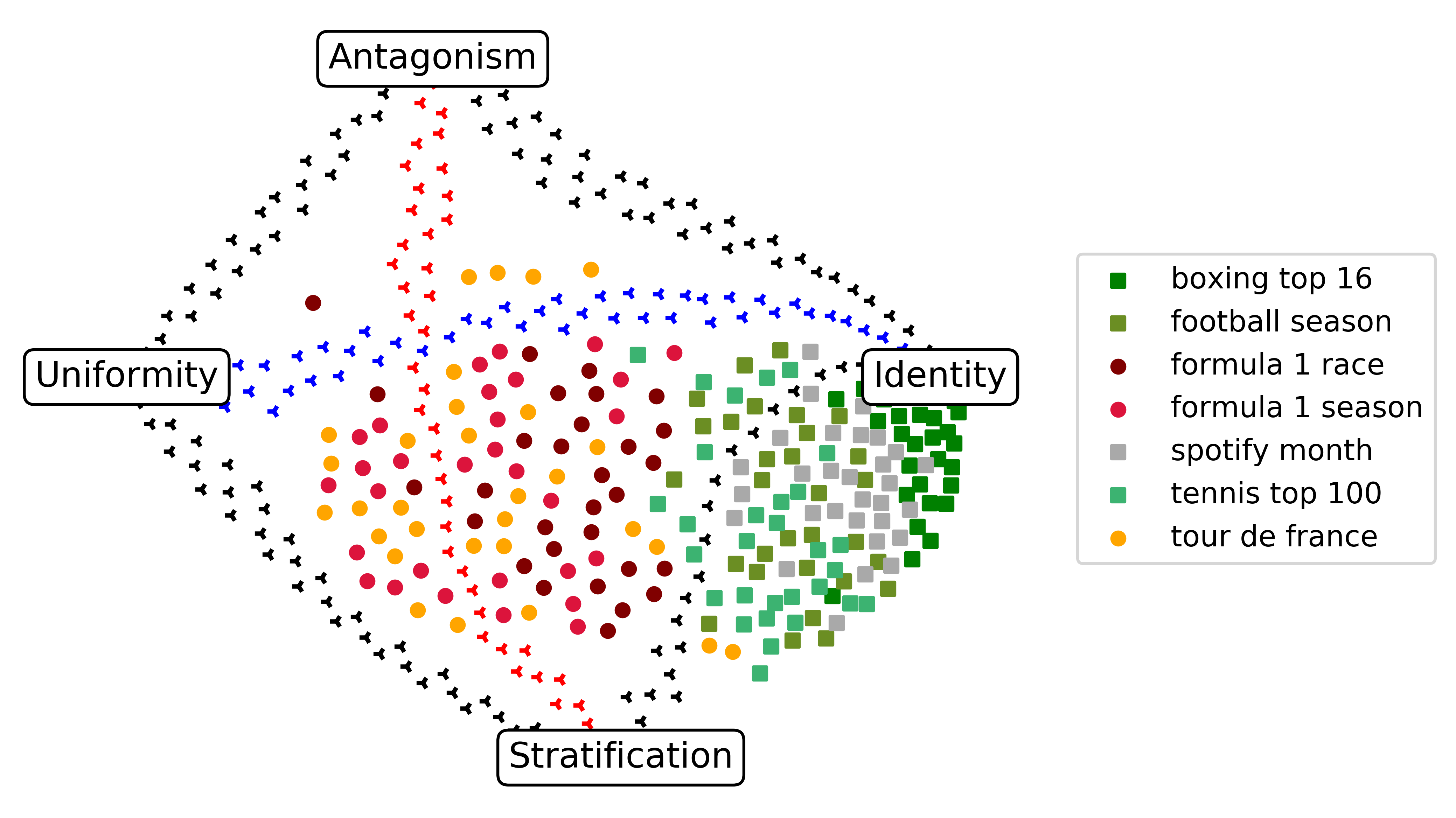
(a) Time-based elections

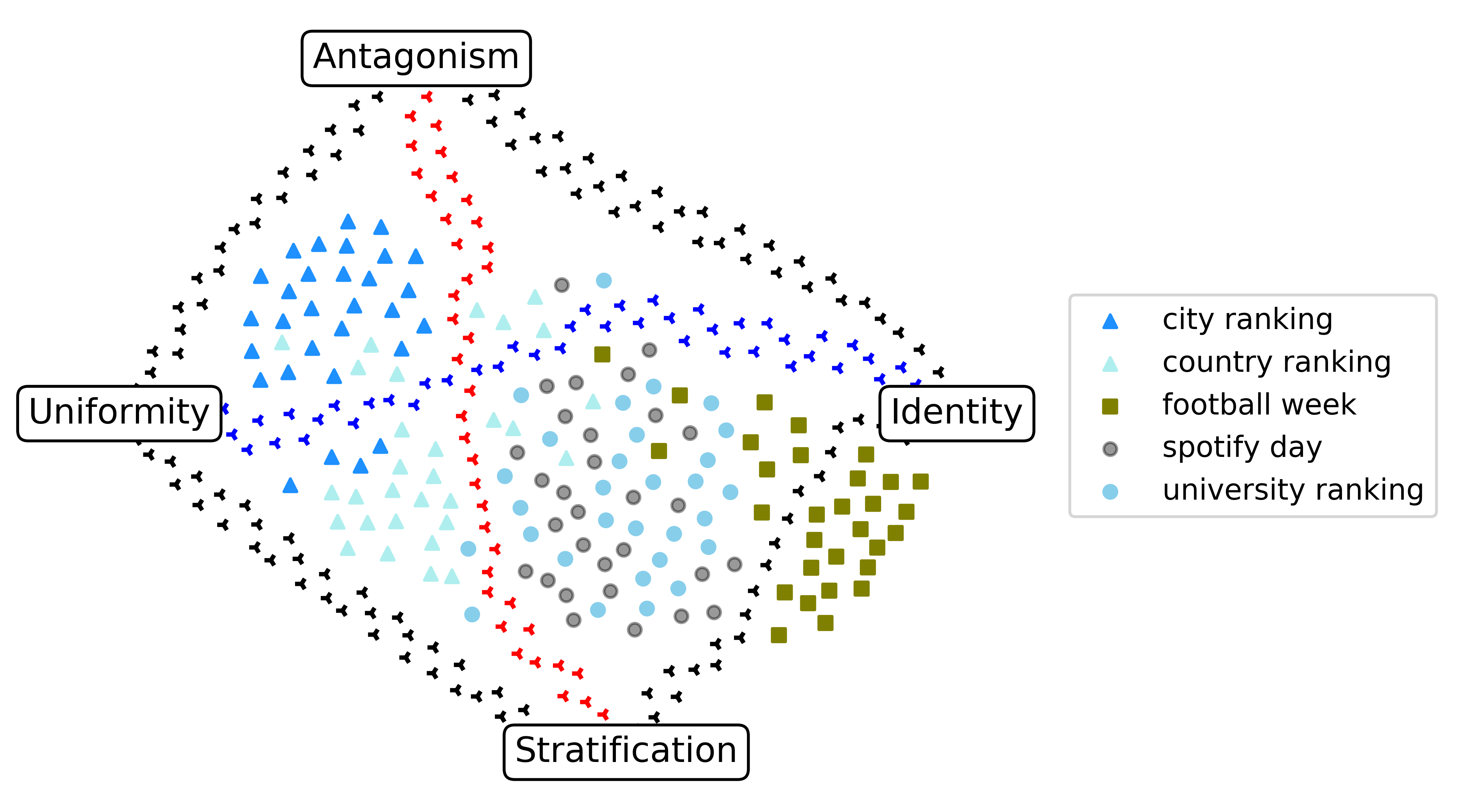
(b) Criterion-based elections

Figure 1: Visualization of our elections as map of elections.

Setup.

We created two maps of elections (Figure 1) where each election is represented by a point whose shape and color indicate the dataset to which it belongs. To make the created maps not too crowded, we created a separate map for time-based (Figure 1(a)) and criterion-based (Figure 1(b)) elections. For each map, we included $30$ elections sampled uniformly at random from each normalized dataset and the compass elections introduced by Boehmer et al. [9] together with their convex combinations appearing as “paths”. Moreover, in Figure 2, we also depict for each pair $A$ and $B$ of datasets, the average positionwise distance of elections from $A$ to elections from $B$ (note that in case we have $A=B$, we take the average over all pairs of elections from $A$). In the last four columns, we show the datasets’ average distance from the compass elections.

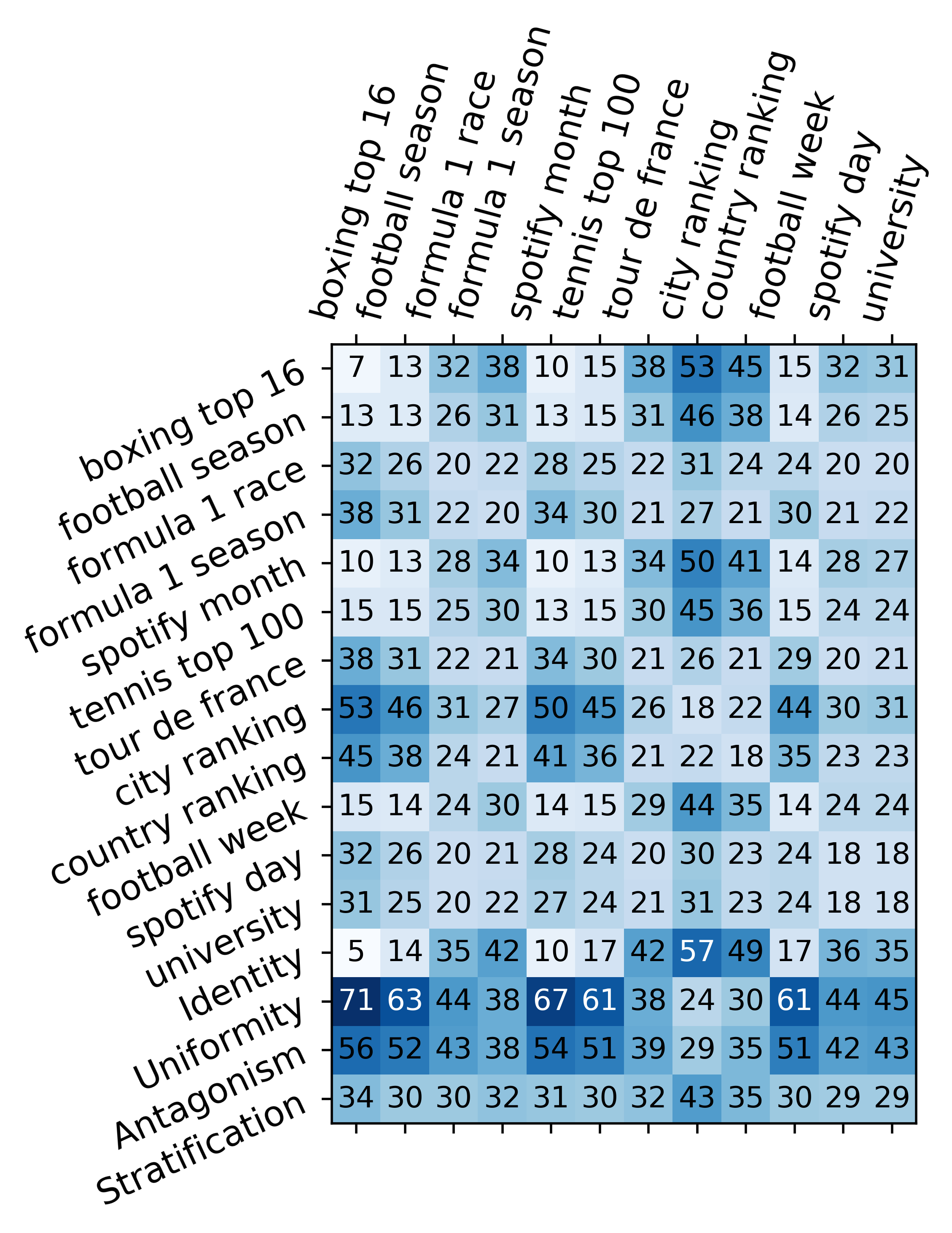
Figure 2: Average positionwise distance of election pairs from different datasets. The maximum distance between two election is $74.67$.

Classifying Datasets.

Examining Figures 1 and 2, it is possible to divide our datasets into three groups: The first group of datasets (boxing top 16, football season, spotify month, tennis top 100, and football week) drawn as squares all contain elections somewhat close to identity (see also Figure 2). Notably, except for football week, these are all time-based datasets. For all of them except spotify month, the ranking at a certain point in time also depends on previous information on candidates that also already influenced previous votes, so in some sense, votes are “by design” not independent here. In contrast to this, in time-based elections from the other datasets (Formula 1 race, Formula 1 season, and Tour de France), which are further away from identity, one vote only depends on the performance of a candidate at some point in time (and not on previous performances)

The second group of datasets (Formula 1 race, Formula 1 season, Tour de France, spotify day, and university rankings) drawn as circles constitute the “middle” part of our maps: This is also reflected in them being roughly at the same distance from identity and uniformity (while all are clearly closer to stratification than to antagonism; see also Figure 2). What is particularly striking here is that despite the fact that these elections are seemingly not all simply close to a canonical extreme election like identity, there are surprising similarities between the datasets: In particular, university, Formula 1 race, and spotify day elections all fall in exactly the same area of the space of elections (the average distance of two elections from one of these datasets is very close to the average distance of two elections picked from two different of these datasets). The same also holds for Tour de France and Formula 1 season elections. Remarkably, Tour de France and Formula 1 season elections are also by design of a very similar nature in the sense that in both datasets players compete in a similar task on different days. The similarity of these datasets indicates that whether players drive in cars or ride bicycles seems to be not so crucial for the resulting election (similar observations apply to boxing top 16 and tennis top 100, and city rankings and country rankings).

The third group of datasets consists of city and country rankings and is drawn as triangles. Both are clearly different from the rest as they are significantly closer to uniformity than identity. Remarkably, the city ranking dataset is the only one of our datasets and the first known dataset which is significantly closer to antagonism (distance $29$) than stratification (distance $43$). Considering the underlying data which provides ratings of cities according to different indicators, the “closeness” to antagonism is quite plausible, as some of the studied indicators seem to capture in some sense contradicting objectives, e.g., big cities where inhabitants typically have access to a variety of healthcare facilities (being one of the indicators) are typically also quite polluted (being another indicator).

Captured Part of the Space of Elections.

It seems that our datasets contain elections of a different nature than those available on PrefLib: Boehmer et al. [9, Figure 2b] drew a map of elections including representatives of all PrefLib datasets with at least $10$ candidates, $10$ votes, and not too many ties. They observed that most elections are closer to uniformity than identity and closer to stratification than antagonism, thereby ending up in the bottom left quadrant of the map. In contrast to this, our elections are mostly located in the bottom right quadrant. Nevertheless, we can confirm the observation of Boehmer et al. [9] that real-world elections typically end up closer to stratification than antagonism (we also do not provide any elections that are in the top right quadrant).

Homogenicity of Elections from one Dataset.

Figures 1 and 2 also shed some light on the “diversity” of elections from one dataset: Looking at the maps, we can observe that while there is some mixing between elections from different datasets, elections from one dataset typically fall into the same area of the map. This indicates a certain kind of shared structure. However, this degree of homogenicity of a dataset, which can be quantified as the average distance of election pairs from this dataset (see “diagonal” entries from Figure 2) depends on the dataset: At the one extreme are boxing top 16, spotify month, and football season with an average distance of $7$, $10$, and $13$, respectively, and on the other extreme are Tour de France, Formula 1 race and Formula 1 season with an average distance of $21$, $20$, and $20$, respectively.

5 Similarity Measures and their Correlation

In addition to our analysis from the previous section based on the map of elections, in this section, we focus on one structural property of our elections, i.e., the similarity of different votes in one election. In Section 5.1, we analyze how similar different votes from one election are using four different metrics and also inspect the metric’s correlation. In Section 5.2, we analyze whether the top part, middle part or bottom part of different votes are more similar to each other. Lastly, in Section 5.3, we restrict our focus to time-based elections and analyze the similarity of successive votes in those elections.

5.1 Similarity Measures and their Correlation

• The NP-hard to compute Kemeny score is always highly correlated with the average KT-distance of all vote pairs and the EMD-positionwise distance from Identity.

• All datasets are quite homogenous with respect to the similarity of votes in elections.

• For most of our elections the values of all similarity measures are not small.

In this subsection, we compare four measures capturing different facets of similarity. Similarity measures are also a potentially attractive parameter to develop parameterized algorithms because they can be understood as a “distance from triviality” parameterization, as most computational problems are easy if all votes are the same (see, e.g., [2]).

Setup.

We consider four similarity measures:

Maximum KT-distance

The maximum KT-distance among all pairs of votes: $\max_{v,v^{\prime}\in{{V}\choose{2}}}{\mathrm{KT}}(v,v^{\prime})$.

Average KT-distance

The average KT-distance among all pairs of votes: $\nicefrac{{\sum_{v,v^{\prime}\in{{V}\choose{2}}}{\mathrm{KT}}(v,v^{\prime})}}{{|{{V}\choose{2}}|}}$.

Disagreeing pairs

The number of candidate pairs for which not all votes agree on their ordering: $|\big{\{}\{c,c^{\prime}\}\in{{C}\choose{2}}\mid\exists v,v^{\prime}\in V:c\succ_{v}c^{\prime}\wedge c^{\prime}\succ_{v^{\prime}}c\big{\}}|$.

Kemeny score

The minimum summed KT-distance of a central order to all votes: $\min_{v^{*}\in\mathcal{L}(C)}\sum_{v\in V}{\mathrm{KT}}(v,v^{*})$.

Note that the number of disagreeing pairs is always at least as large as the maximum KT-distance, which in turn is at least as large as the average KT-distance (all three values range from $0$ to $|{{C}\choose{2}}|$ so from $0$ to $105$ in our case).

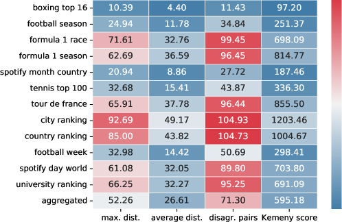
Figure 3: Average values for four different similarity measures. Colors encode the values normalized by the theoretically possible maximum value.

Values of Similarity Measures.

In Figure 3, for all four measures, we depict for each dataset the value of the similarity measure averaged over all $500$ elections from the dataset. Concerning the results on the aggregated dataset, what stands out is that the maximum KT-distance and the number of disagreeing pairs is quite high and in particular much higher than the average KT-distance (and comparing normalized values also than the Kemeny score). However, this is also quite intuitive in the sense that both the maximum distance and the number of disagreeing pairs might in the end only depend on two voters and are thus very sensitive to “outliers” (as soon as there are two voters with reversed preferences orders in an election, both values are at the maximum). Considering the results on the different datasets, especially the average number of disagreeing pairs clearly divides them (in line with our groups proposed in Section 4): Unsurprisingly, the datasets close to identity have a “low” average number of disagreeing pairs (always below 50). The number is the lowest for boxing top 16 and spotify month with $11.43$ and $27.72$, respectively. This is quite remarkable as it means that all voters agree on the ordering of $89.1\%$ and $73.6\%$ of all candidate pairs, respectively. For the “middle” datasets, the average number of disagreeing pairs is much higher and lies between $89.8$ and $99.45$ (this means that the voters only agree on the ordering of between $5.4\%$ and $14.4\%$ of all candidate pairs). For the two “outliers”, city and country ranking, the average number of disagreeing pairs is very close to the maximum possible value of $105$ with $104.93$, respectively, $104.73$. As already discussed in Section 4 one reason for this might be that in the two “outlier” datasets votes correspond to sometimes contradicting and opposing indicators, which can lead to two close-to-reversed votes.

Interestingly, for all considered datasets, a majority of elections from the dataset have close similarity scores. That is, for all four measures, the median and average value are nearly identical and the first and the third quantile differ only by around $10\%$ from the median.

Similarity Measures for Parameterized Algorithms.

Betzler et al. [2] developed different parameterized algorithms for computing the central order minimizing the Kemeny score: One algorithm running in $\mathcal{O}^{*}(2^{m})$, where $m$ is the number of candidates. Another algorithm running in $\mathcal{O}^{*}(1.53^{k})$ where $k$ is the Kemeny score, and an algorithm running in $\mathcal{O}^{*}(16^{d})$ where $d$ is the average KT-distance (they also considered the maximum KT-distance between two votes as a parameter for a related problem). Considering the average values on the aggregated dataset, the exponential part of the running time of these algorithms evaluate as follows. $2^{m}$ is $32768$, $1.53^{k}$ is $7.79\text{\times}{10}^{109}$, and $16^{d}$ is $1.1\text{\times}{10}^{32}$. Even on boxing top 16, where votes are most similar to each other, the number of candidates still leads to the best results ($2^{m}$ is $32768$, $1.53^{k}$ is $8.2\text{\times}{10}^{17}$, $16^{d}$ is $198668$), partly questioning the practical usefulness of the algorithms for the two similarity parameterizations. Overall, it seems that the number of candidates is nearly always the best of our parameters to use. Considering the different similarity measures, the average KT-distance is clearly the smallest, which is also theoretically guaranteed; however, the gap to the other parameters might be seen as unexpectedly large.

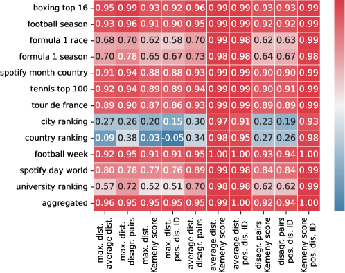
Figure 4: Correlation of similarity measures. Colors represent the respective value (blue means $0$; read means $1$).

Correlation of Similarity Measures.

We also computed for each pair of metrics their Person correlation coefficient (see Figure 4). Here we also considered election’s EMD-positionwise distance (see Footnote 7) from the Identity election, where all voters have the same preferences. Recall that this distance was also essential for our previously proposed classification of datasets. For all our datasets, the correlation between the average KT-distance and the Kemeny score is between $0.97$ and $1$ (the detected linear relationship here is that the Kemeny score of an election is $23.8$ times the average KT-distance minus $37.8$). Moreover, the EMD-positionwise distance from Identity is similarly strongly correlated to the Kemeny score with a PCC value of $1.00$ on the aggregate dataset and PCC values ranging from $0.93$ to $1$ on the level of individual datasets (the detected linear relationship here is that the Kemeny score of an election is $21.6$ times the EMD-positionwise distance plus $53.8$). This indicates that in most practical applications where one is interested in the NP-hard to compute Kemeny score, it is sufficient to simply compute the average KT-distance or the EMD-positionwise distance from Identity. Accordingly, the correlation between the EMD-positionwise distance and the average KT-distance is also similarly high. For the other pairs of metrics, the correlation on the aggregate dataset is again very high ranging from $0.93$ to $0.96$, which is quite surprising given the different nature of the measures (also in terms of how sensitive they are to outliers). However, here there are some differences on the dataset level: The two examples where the correlation is the lowest are city and country elections, where all pairs of metrics except the three pairs discussed above have a linear correlation between only $0.03$ and $0.34$. This, again, might be due to the fact that in these datasets votes are sometimes reverses of each other. This severely affect the maximum KT-distance and the number of disagreeing pairs yet only partly increase the average KT-distance, Kemeny score, and EMD-positionwise distance from Identity. However, it remains unclear why also the correlation between the number of disagreeing pairs and the maximum KT-distance is quite low here.

5.2 Similarity in Different Parts of Votes

• Voters typically agree more on which candidates should be considered as high-quality or low-quality candidates than who should be considered as medium-quality candidates.

• Voters tend to rank candidates at the top more consistently in the same ordering than candidates at the bottom.

Having analyzed the general similarity of votes in one election, we now ask whether certain parts of votes exhibit a higher similarity than others. For this, we divide each vote (consisting of $15$ candidates) into three parts each containing $8$ candidates: the top part capturing positions one to eight, the middle part capturing positions five to twelve, and the bottom part capturing positions eight to fifteen (note that the different parts partly overlap).

Setup.

For each election and each of the three parts, we computed two similarity measures:

Pairwise intersection

We compute for each pair of votes the number of candidates that appear in both votes in the considered part. The pairwise intersection is this value averaged over all pairs of votes in the election.

Total intersection

Number of candidates that appear in all votes in the considered part.

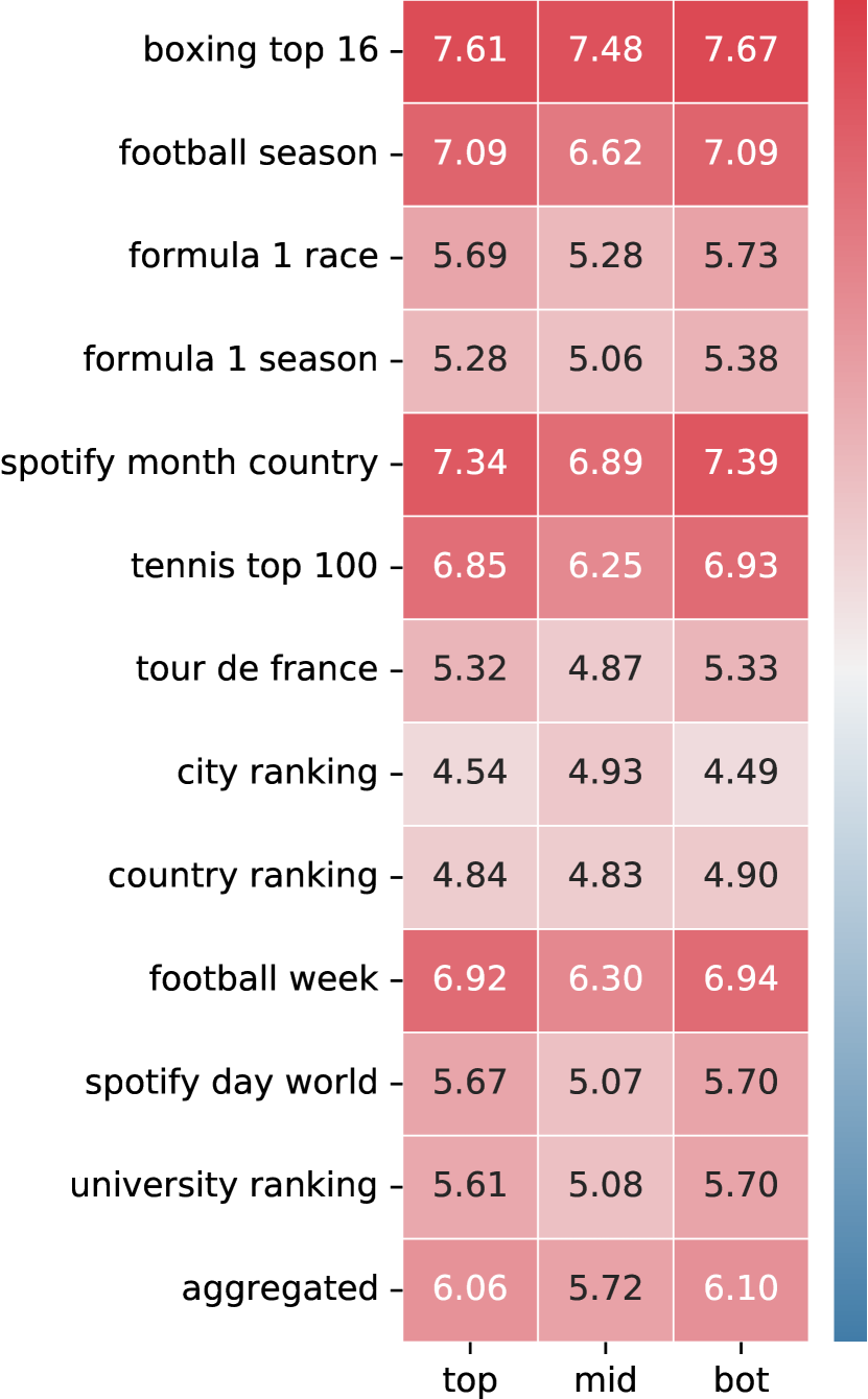
(a) Pairwise intersection.

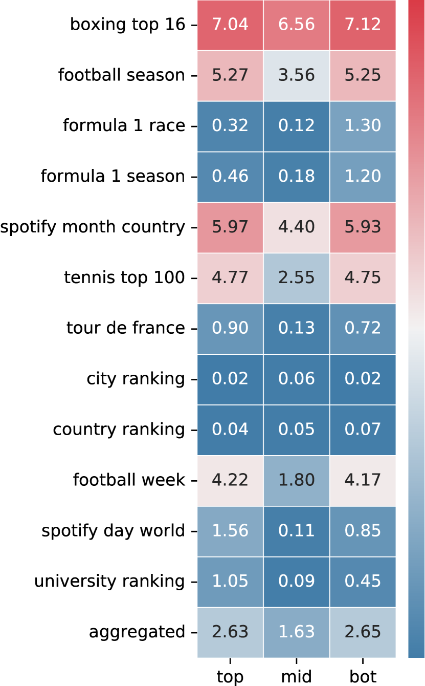
(b) Total intersection.

Figure 5: For each dataset, for two different similarity measures, average values for the three parts of the votes.

Results.

Averaged over all elections, the pairwise intersection in the top, middle, and bottom part is $6.06$, $5.27$, and $6.1$, respectively, while the total intersection is $2.63$, $1.63$, and $2.65$, respectively (see Figure 5 for separate results for each dataset). Recalling that each constructed part consists of eight candidates it is remarkable that each pair of votes roughly agrees on six candidates in each part. This indicates a high pairwise consensus of voters on the general quality of candidates in all of our elections. In contrast to this, the number of candidates appearing in all votes in the same part is quite low, indicating a lower overall consensus. However, datasets that are close to identity also exhibit a high overall consensus, i.e., the total intersection for the top and bottom part ranges from $4.17$ to $7.12$, whereas for the middle part the values are a bit lower ranging from $1.8$ to $6.56$.

Comparing the different parts of the votes to each other, for all datasets except city rankings, the average and total intersection for the top and bottom part is higher than for the middle part. This suggests that while voters have similar opinions about who should be considered as a high-quality or low-quality candidate, opinions are more diverse concerning medium-quality candidates. The difference is particularly strong for football week elections where the total intersection for the top and bottom part is $4.2$, but only $1.8$ for the middle part. Recalling that football week elections are based on power rankings of football teams published by different media outlets in the same week this is also quite intuitive, as there are typically some clearly strong and clearly weak teams that appear in the top, respectively, the bottom of each ranking, while the middle part is more subjective.

The general trend that voters in most of our elections agree more which candidates should be ranked on the top or the bottom than in the middle also provides a possible justification why a great majority of our elections is closer to stratification than to antagonism (as discussed in Section 4). Under antagonism, half of the voters rank the candidates in one order and the other half of the voters rank them in the opposite order. Consequently, all voters agree on which are the medium-quality candidates while the electorate is divided concerning who are the best and worst candidates. This is exactly the opposite of what we observe in our data.

For the top and bottom part of elections from datasets close to identity, the total intersection value is large enough to also meaningfully analyze whether voters opinions about the ordering of candidates are more similar at the top or at the bottom: For this we computed for each election the average KT-distance between two votes restricted to the candidates appearing in all votes in this part. The results clearly indicate a stronger consensus at the top than at the bottom, in particular in boxing top 16 and tennis top 100 elections. For these two datasets this can be explained by the fact that in these elections it should be much more difficult to climb up on position when you are in the top part (you are one of the best players) compared to when you are in the bottom part (you are one of the worst ranked players).

5.3 Similarity in Time-Based Elections

• For all time-based datasets except Formula 1 season, Formula 1 race and Tour de France, votes that appear closer to each other in time are more similar to each other.

• In time-based elections, candidates ranked in first and last position change less frequently than the candidates in other positions.

For time-based elections, votes have a natural ordering which makes it possible to analyze the change of votes over time. In this section, we do not consider the normalized datasets (because they have no ordering); instead, for each raw election from a time-based dataset, we deleted all candidates that do not appear in all votes and subsequently discarded the election if less than $10$ candidates remain (it is important that we do not delete voters, as we also analyze the change between one voter and the following; we call two such voters successive).

Setup.

For each election, we computed the following:

Average ordering change

The average number of times the pairwise ordering of two candidates is swapped over time.

Maximum ordering change

The maximum number of times the pairwise ordering of any two candidates is swapped over time.

Average fluctuation

For each position, we compute the number of votes where the candidate on this position is different in the next vote. The average fluctuation is this value averaged over all positions.

Notably, the average ordering change value times the number of candidate pairs gives the summed KT-distance of all pairs of successive votes.

However, evaluating the values of these measures without additional information is very difficult, as the observed values might simply be due to the structure of the election and not due to the ordering of the votes (for instance, if two candidates have the same pairwise ordering in all but one vote then it is nearly irrelevant how the votes are ordered for our measures, while if they are ranked in the same order in half of the votes and in the opposite order in the other half, then the ordering of votes truly makes a difference). That is why, for each considered election, we created a copy where we shuffled all votes randomly and recomputed the above quantities. The average values for each dataset can be found in Table 2.

name	original					shuffled
	Avg. ord. ch.	Max. ord. ch.	Avg. fluct.	Cor. KT+temp.		Avg. ord. ch.	Max. ord. ch.	Avg. fluct.
boxing top 16	0.82	2.82	2.7	0.7		1.97	10.08	14.98
football season	1.14	5.15	10.3	0.46		1.49	6.24	11.09
Formula 1 race	8.96	15.84	45.98	0.04		11.96	18.57	49.75
Formula 1 season	4.05	7.26	14.52	0.03		4.08	7.17	14.53
spotify month	1.22	9.38	22.54	0.86		1.92	11.64	25.64
tennis top 100	1.31	6.86	23.16	0.93		4.43	16.9	42.79
Tour de France	4.63	9.27	19.47	0.05		4.84	9.44	19.53

Table 2: For each dataset, average values of time-based similarity measures for original and shuffled elections and correlation between KT- and temporal distance.

Lastly, for each dataset, we also computed the correlation between the KT- and temporal distance of two votes. For this for each pair of votes in some election from this dataset, we computed the KT-distance and the temporal distance (as the number of votes that come in between the two plus one). Afterwards we computed the PCC of these values. The results can be found in fifth column of Table 2.

Results.

We first discuss the ordering change. Comparing the results for the original and shuffled elections in Table 2, no clear difference is visible for Formula 1 season and Tour de France elections (remarkably, both datasets capture similar types of elections where players compete in multiple stages on different days against each other). This indicates that in elections from these datasets the time-based ordering of the vote does not have any direct consequences on the votes, i.e., performances of candidates in one stage have no clear connection to their performance in the next stage. For all other datasets, the time-based ordering induces a more “structured” election than a random ordering, indicating that successive voters have some form of relationship here. The most extreme example is tennis top 100, where following the true order of the votes the ordering of each candidate pair only changes $1.31$ times, on average, while following a random order it changes $4.43$ times. That votes have a strong temporal relationship in these elections can be explained by considering the design of the underlying ranking: Players gain points based on their performance in major tournaments and keep them for roughly one year. Thus, the number of points a player has typically does not drastically change between weeks (each corresponding to a vote) implying some form of temporal consistency. However, also in elections that are subjected to a higher degree of change such as Formula 1 race elections the temporal dimension of the data is visible: In the original elections, the ordering of the candidates (which in this context means which of the candidates needed less time for the respective lap in the underlying race) changes on average $8.96$ times, while if we shuffle votes (laps) then it changes on average $11.96$ times.

(a) Fluctuation on different positions.

(b) KT-distance of successive votes.

Figure 6: Time-based similarity in football season elections. Taking into account that elections have different sizes, we mapped the results for all elections on the average election size and afterwards averaged them to obtain the depicted graphs. In blue, the original data is shown; in orange, the shuffled data.

Next, for each dataset separately, we consider the PCC of the KT-distance and the temporal distance of each pair of votes in the election as an additional simple measure for the temporal correlation of the votes. Here, again, in the Formula 1 season and Tour de France data, no correlation is visible. Moreover, this metric also indicates that slightly contrary to our previous observations, there is nearly no linear correlation between the KT- and temporal distance of votes in the Formula 1 race data. In contrast to this, for boxing top 16, spotify month and tennis top 100, the correlation is strong. For tennis top 100, the correlation value is even $0.93$, indicating a close to perfectly linear correlation.

We also examined the average fluctuation for different positions. Here, it is typically the case that the first and last positions exhibit less fluctuation, indicating that in time-based elections changes on the first and last position are rarer than changes on other positions. We show in Figure 6(a) an exemplarily plot for football season elections. Moreover, we also analyzed the KT-distance between successive votes: While for most datasets no clear relationship between the index of votes in the election (i.e., whether it is the first, second, third, … vote in the election) and its KT-distance to its successive vote is visible, football season elections form a clear exception: In these elections, the average KT-distance between successive votes is usually around $125$ but drops to around $100$ for the last votes (see Figure 6(b) for a visualization). Recalling that each vote here represents the power ranking of football teams in different weeks of the season (with the first vote representing the first ranking and the last vote the final ranking) this is quite plausible because typically teams need some time within a season to show their “true” quality.

6 Restricted Domains

• There are only few elections from a restricted domain and only some elections close to one.

• Elections that are close to one domain are typically also close to another.

• Elections from a restricted domain are typically quite degenerate.

In this section, we analyze which of our elections are part of a restricted domain. There are numerous papers analyzing the computational complexity of various problems on elections from different types of restricted domains (see e.g., [73, 3, 34, 38, 77, 11, 50, 28] and Elkind et al. [27, 29] for surveys). Possible motivations for these works are typically that restricted domains allow for nice combinatorial algorithms and the belief that they capture (close-to) realistic situations. We focus on the three arguably most popular restricted domains of single-peaked [5], single-crossing [57, 68], and group-separable elections [44, 43].

We check here which of our elections fall into one of these domains and afterwards consider the candidate deletion and voter deletion distance of all elections from them.

Members in Restricted Domains.

Overall, only very few of our elections fall into a restricted domain. That is, for the $500$ boxing top $16$ elections, where votes are very similar to each other, the number of single-peaked/singe-crossing/group-separable elections is $77$/$138$/$101$. Moreover, we have one single-peaked election in the football season dataset and one in the spotify month dataset. So overall, only $1.3\%$, $2.3\%$, $1.6\%$ of our elections are single-peaked, single-crossing, and group-separable, respectively. Some other works have also analyzed the occurrences of elections from restricted domains and found even less evidence: Regenwetter et al. [67] analyzed five-candidate American Psychological Association (APA) presidential elections and found no evidence of restricted domains. Mattei [52] considered three- and four-candidate elections based on a Netflix price competition and found that $0.03\%$ of elections are single-peaked.

Distance to a Restricted Domain.

Given that only a few of our elections fall into a restricted domain, our goal now is to check whether more are at least close to one. In particular, we consider the voter deletion and candidate deletion distance, i.e., the minimum number of voters/candidates that need to be deleted such that the resulting election falls into the restricted domain. Notably, there are also many more distance measures (see, e.g., [31, 22, 26]). Moreover, motivated by the many polynomial-time results on restricted domains, there are several papers developing parameterized algorithms for election-related problems for different distance measures to restricted domains (see [35, 56, 58] for algorithms parameterized by the voter and candidate deletion distance and [22, 85, 84, 83, 73] for examples for other distance measures).

(a) aggregated

(b) spotify month

(c) spotify day

Figure 7: For different datasets, fraction of elections within a given candidate deletion (solid) or voter deletion distance (dashed) from single-peakedness (blue), single-crossingness (orange), and group-separability (green).

For each of our elections, we computed the voter and candidate deletion distance from single-peakedness, single-crossingness, and group-separability. In Figure 7(a), we show the results on the aggregated dataset as a cumulative distribution function. For the candidate deletion distance, the picture is very similar for all three restricted domains: There are around $15\%$ of elections within distance $4$, around $28\%$ within distance $6$, around $56\%$ within distance $10$, and around $99\%$ within distance $12$. Considering that we have seen in the previous part that there are considerably more single-crossing elections than single-peaked or group-separable elections, the similarity between the domains here is partly unexpected.

For voter deletion, there is some difference between the restricted domains: For all three restricted domains, $15\%$ of elections are within distance $14$ and are more or less uniformly distributed within this distance. For single-peakedness and group-separability, $25\%$ of all elections are within a distance of $18$, $50\%$ within a distance of $23$, and $99\%$ within a distance of $27$. For single-crossingness, distances are typically one smaller, as $25\%$ of all elections fall within distance $17$ and $50\%$ within distance $20$. This slight difference might be because in contrast to the other two domains, for single-crossingness an ordering of the voters is needed which might be easier to construct if we can choose which voters to delete (however, for single-peakedness the same is true for candidate deletion, yet no such effect is visible). Comparing the normalized voter deletion distance to the normalized candidate deletion distance it seems that the latter is typically slightly smaller. Nevertheless, there is a strong linear correlation between the candidate deletion and voter deletion distance of an election.

Examining the results on the dataset level, there are significant differences: The general trend here is that the higher the average Kemeny score of a dataset is the further is the dataset on average from a restricted domain. One dataset from our close to identity group which contains many elections with a low Kemeny score are spotify month election, and in Figure 7(b) we depict the cumulative distribution for this dataset. Notably, for all three restricted domains, elections from this dataset have the second-lowest candidate deletion distance, i.e., $50\%$ of the spotify month elections have a candidate deletion distance of $5$ and smaller. In contrast to this, in Figure 7(c) we show the plot for spotify day elections which belong to the middle datasets and have higher Kemeny scores. Here for all elections, at least $9$ candidates or at least $21$ voters need to be deleted to make it fall into one of our three restricted domains, indicating that this dataset is far away from a restricted domain. Given that one can see the whole spotify data as one huge election, the opposite behavior of spotify day and spotify month elections highlights the natural fact that depending on which votes from a large election are taken into account very different elections arise. To sum up, we have found only little evidence of elections from restricted domains and also only a few elections at a small distance (recall that $5$ candidates are not really a small number here, as this corresponds to $33\%$ of candidates). Thus, both the voter and candidate deletion distance are probably too large on many real-world elections for the usage of parameterized algorithms.

To the best of our knowledge, the work of Sui et al. [75] is the only other work that studies the distance of real-world elections from a restricted domain. In particular, they analyzed two large elections (both with $9$ candidates and over $10\,000$ votes) related to the 2002 Irish general election and found that for both more than $95\%$ of voters need to be deleted to make the election single-peaked. This indicates that our elections are comparably quite close to a restricted domain (which also might be due to the case that we have fewer voters). Moreover, they also considered the minimum number of axes such that each vote is single-peaked with respect to one axis and found that for one election more than $36$ and for the other more than $263$ axes are needed. On the positive side, they found that the voter deletion distance of their two elections to, so-called, two-dimensional single-peakedness is much smaller. Testing how far our elections are from multi-dimensional single-peakedness would be an interesting direction for future work.

Membership in Multiple Restricted Domains.

Motivated by previous works by Skowron et al. [73] and Elkind et al. [30] on elections that are simultaneously single-peaked and single crossing and to better understand the relationship of the different restricted domains, we now analyze whether elections that are part of, or close to, one restricted domain are typically also part of or close to another. In Figure 8(a), we show a Venn diagram capturing all elections that are part of one of our three restricted domains: Each domain is represented by a circle and the overlap of different circles (and the numbers shown there) represents the intersection of domains. Notably, each restricted domain shares more elections with another domain than there are elections that are only part of this domain. In fact, there are almost as many elections that are part of all three domains ($37$) than elections that are single-peaked or group-separable but not single-crossing ($43$). This indicates that in practice there is a significant overlap of the domains and that algorithms for single-crossing elections can be applied to most elections falling in one of the three domains.

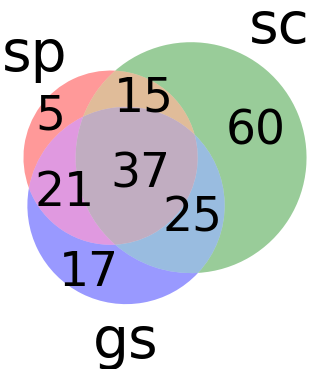
(a) VD/CD 0

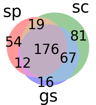
(b) CD 1

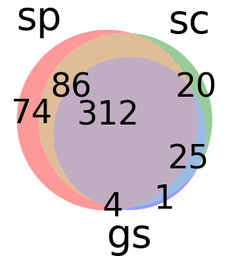
(c) CD 2

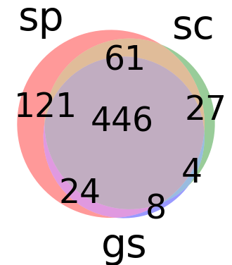
(d) CD 3

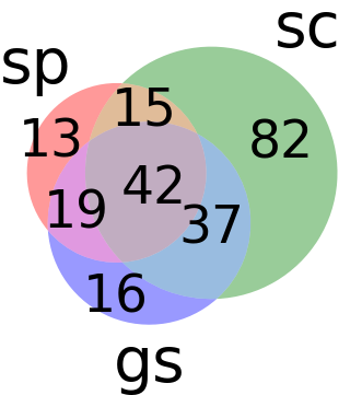
(e) VD 2

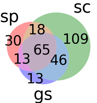
(f) VD 4

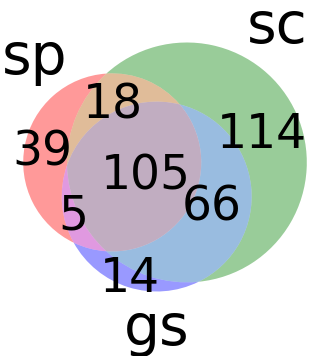
(g) VD 6

Figure 8: For different voter deletion distances (VD) or candidate deletion distances (CD), Venn diagrams of elections which are within the given distance from single-peakedness, single-crossingness, or group-separability.

In Figure 8, we also display Venn diagrams for elections that are within a certain voter or candidate deletion distance from a restricted domain. Elections that are close to one of the domains after deleting some candidates overlap even more than elections from restricted domains: Remarkably, considering elections within a candidate deletion distance of $3$, there are $3.5$ times more elections that are within this distance from all restricted domains, than those that are only close to one restricted domain. For the different voter deletion distance values the picture is roughly similar as in Figure 8(a). So overall it seems that in real-world elections the different restricted domains and their closer environment heavily overlap and that it is, for instance, possible to apply algorithms for (close to) single-peaked or single-crossing elections to an overwhelming majority of (close to) group-separable elections.

Moreover, there is also a strong linear correlation between an election’s distance from the different restricted domains: For each pair of our restricted domains, the Pearson correlation coefficient of the candidate deletion distances from the two is around $0.95$, while it is between $0.85$ and $0.9$ for the voter deletion distance.

Further Considerations.

In Section B.1, we analyze the properties of elections that are (close to) being single-peaked or single-crossing and observe that they are typically quite degenerate, meaning that they have a low Kemeny score and that they fall into a small part of the space of all elections from the respective restricted domain. For single-peaked elections, we find that the top-choices of voters typically fall in the same area of the societal order. Moreover, in Section B.2, we check which of our elections fulfills some more general restrictions. Among others, we find that value-restricted elections [70] occur quite frequently and that in the characterization of single-peaked, single-crossing, and group-separable elections via forbidden configurations one of the two configurations is redundant in practice.

7 Case Study: How Different are Different Voting Rules?

In this section, we use our datasets to shed some further light on traditional questions from social choice. While there is already quite some empirical research on the considered questions, nearly all of these works considered elections with $3$ to $5$ candidates coming from a single data source. Thus, our rich data allows us to take a broader look.

One popular question arises around the notion of a Condorcet winner. A candidate $c$ is a strong (weak) Condorcet winner if for each other candidate $d$ more than (at least) half of the voters prefer $c$ to $d$. Previous research has found that strong Condorcet winners nearly always exist, i.e., the so-called Condorcet paradox occurs relatively rarely, and that the strong Condorcet efficiency, i.e., how often these rules select the strong Condorcet winner as a winner, of all rules is very high [52, 18, 23, 64, 63]. We investigate these issues in Section 7.1.

In Section 7.2, we analyze the level of agreement between different voting rules. While from a theoretical and axiomatic perspective, voting rules significantly differ from each other, various authors provided evidence that most of them are very similar in practice [52, 18, 39, 66, 67, 55, 23, 64].

Overall, while parts of our results in this section are in line with previous studies, we also find evidence that suggests that the established consensus in the literature according to which in practice all voting rules are more or less the same should be relativized, as it seems to only apply if we have elections with a Condorcet winner and/or the number of voters divided by the number of candidates is large.

We start by defining all considered voting rules (for each rule computing a score, all candidates with the highest score win.):

Plurality

Each voter awards one point to its top-choice.

Plurality with runoff

In the first round, each voter awards one point to its top-choice. If more than two candidates have the highest number of points, then delete all but them. Otherwise, we delete all candidates who do not have the highest or second-highest number of points. In the second round, each voter awards one point to the remaining candidate it ranks highest.

Borda

For $i\in[m]$, each voter awards $m-i$ points to the candidate it ranks in the $i$th position.

Copeland

A candidate $c\in C$ gets a point for each candidate $d\in C\setminus\{c\}$ for which a strict majority of voters prefers $c$ to $d$ and loses a point if a strict majority prefers $d$ to $c$.

Hare

In each round, each voter awards one point to its most preferred remaining candidate. After each round, a candidate with the lowest score gets deleted (ties are broken according to the preferences of the first voter). If all candidates in some round have the same number of points, then we return all of them as the winners.

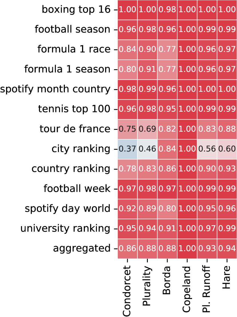
(a) Strong Condorcet winner.

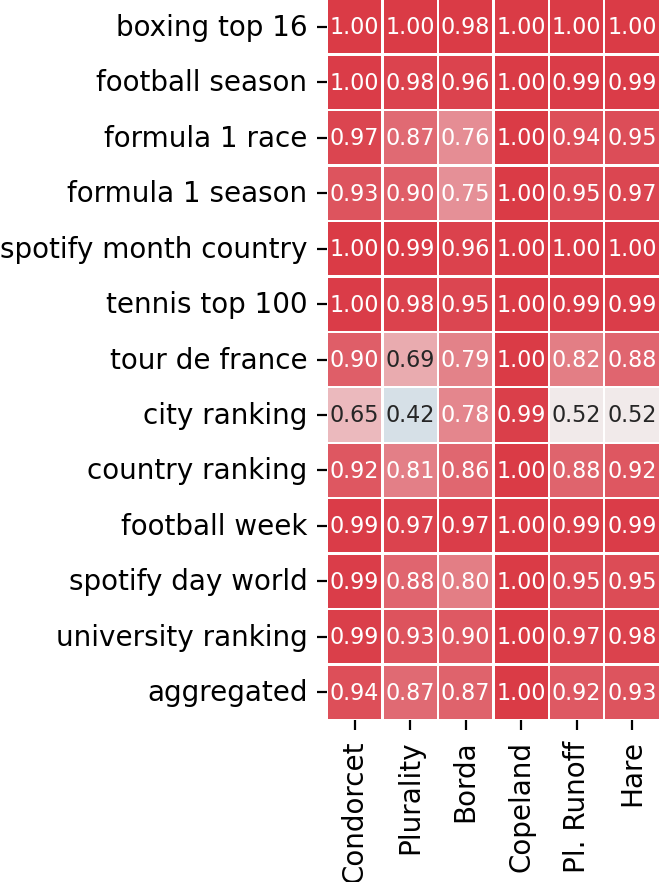
(b) Weak Condorcet winner.

Figure 9: In the first column, fraction of elections admitting a strong/weak Condorcet winner. In the other columns, strong/weak Condorcet efficiency of different voting rules.

7.1 Condorcet Paradox and Condorcet Efficiency

• Most of our elections ($86\%$) have a strong Condorcet winner and all voting rules select them as a winner most of the times ($88\%$ or more).

• In some of our datasets only few elections have a strong Condorcet winner and voting rules select it as a winner less frequently.

In line with the literature, we first focus on strong Condorcet winners. In Figure 9(a), in the first column, we depict for each of our datasets the fraction of elections admitting a strong Condorcet winner. While for all datasets from our first group of close to identity datasets around $96\%$ of elections admit a strong Condorcet winner, for the other datasets this fraction is (considerably) below $100\%$. The most extreme case are city ranking elections where only $37\%$ of the elections admit a strong Condorcet winner. Moreover, overall “only” $86\%$ of all our elections admit a strong Condorcet winner. This is in contrast to previous works. For instance, Popov et al. [64] reported that in one of their studied datasets $6.7\%$ of elections do not admit a strong Condorcet winner, while for all others this value is below $0.3\%$.

Concerning the strong Condorcet efficiency of the different voting rules, results again significantly depend on the considered dataset. For close to identity datasets all voting rules have a very high Condorcet efficiency of $0.95$ and above (note that Copeland’s voting rule is guaranteed to select a strong Condorcet winner if one exists). Mattei [52] and Popov et al. [64] also reported a Condorcet efficiency of $0.95$ and above for different rules. However, on our other datasets, the Condorcet efficiency can be much lower: For Plurality, Plurality with Runoff, and Hare, their Condorcet efficiency is the lowest on the city ranking dataset with $0.46$, $0.59$, and $0.6$, respectively. For Borda, the minimum Condorcet efficiency is $0.77$ on Formula 1 race and Formula 1 season elections. Interestingly, the other voting rules achieve a much higher efficiency on these two sets. Considering the results on the aggregated dataset, Hare and Plurality with Runoff have the highest Condorcet efficiency with $0.94$ and $0.93$ respectively, while Plurality and Borda both have a Condorcet efficiency of $0.88$. Given that Borda takes much more information into account than Plurality, it is slightly unexpected that both perform so similarly here.

In Figure 9(b), we depict the same statistics for the notion of weak Condorcet winners: A substantial fraction of our elections, i.e., $8\%$ of all elections, $15\%$ of tour de France, and $28\%$ of city ranking elections, admit a weak but no strong Condorcet winner. This is quite remarkable given that the distinction between a weak and a strong Condorcet winner almost appears like a tie-breaking issue. The Condorcet efficiency of our rules slightly decreases when moving from strong to weak Condorcet winners. This is something to be expected because weak Condorcet winners, which are now also taken into account, have in general a slightly weaker standing in the election than strong Condorcet winners.

7.2 Consensus among Voting Rules

• Voting rules often agree on the returned winner because most elections have a Condorcet winner and voting rules often select them.

• On elections without a Condorcet winner, Borda and Copeland, on the one hand, and Plurality, Plurality with Runoff and Hare, on the other hand, regularly agree on a winner.

• The rankings returned by different voting rules do not exhibit a strong correlation (and in some cases even none).

In Section 7.2.1, we analyze the consensus among winners returned by different voting rules. After that in Section 7.2.2, we analyze the relationship between the rankings returned by the different voting rules.

7.2.1 Winner Consensus

In Figure 10(a), we depict the average lexicographic agreement of each pair of rules. The average lexicographic agreement of some pair of rules is the fraction of all elections where the winner returned by the two rules is the same if we apply lexicographic tie-breaking during the execution of both rules. In general, the consensus among the different voting rules is quite high, ranging from $0.96$ for the only two iterative rules, Hare and Plurality with runoff, to $0.74$ for Borda and Plurality. However, the reason for this generally high agreement between voting rules might be connected to our observation from Section 7.1 that most of our elections have a strong Condorcet winner and that in case a strong Condorcet winner exists, most of the time rules return it as a winner. To verify this, in Figure 10(b), we depict the average lexicographic agreement of pairs of voting rules on all elections without a strong Condorcet winner. Indeed, the consensus among voting rules is significantly lower in this case: For all pairs of rules except for Hare and Plurality with runoff, whose average lexicographic agreement is still $0.82$, the average lexicographic agreement drops by between $0.27$ and $0.48$ when moving from the full election dataset to elections without strong Condorcet winner. Figure 10(b) further suggests that there exist two groups of voting rules: Plurality, Plurality with Runoff, and Hare on the one hand, and Borda and Copeland on the other hand. This partition is also quite intuitive, as all rules from the first group use Plurality scores in some way or the other, while Copeland and Borda in some sense always take into account the full election. Overall, our results indicate that a main reason why voting rules seem to typically exhibit a high consensus is because they all favor strong Condorcet winners which often exist. This could also explain why previous research [18, 39, 66, 67, 23, 64] has found a higher consensus among rules than what we have observed: On their data strong Condorcet winners exist more often than on ours.

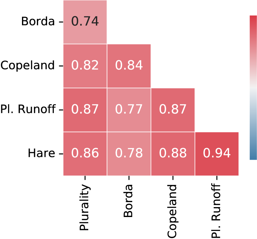
(a) All elections.

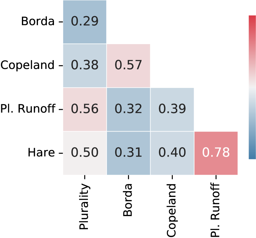
(b) All elections without a strong Condorcet winner.

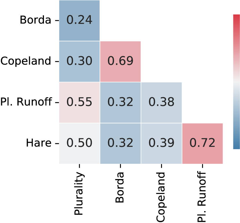
(c) All city ranking elections.

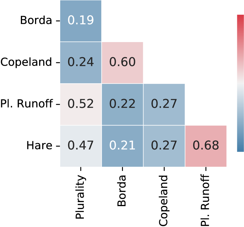
(d) All city ranking elections without a strong Condorcet winner.

Figure 10: For pairs of voting rules, fraction of elections where rules return same winner after lexicographic tie-breaking.

On the dataset level, results are again very different and correlate with our grouping of the datasets: On the one hand, on close to identity datasets the consensus of voting rules is very high, while, on the other hand, on city rankings it is lowest. In Figures 10(c) and 10(d), we display the average lexicographic agreement on all city ranking elections and on all city ranking elections without strong Condorcet winners. Both Figures 10(c) and 10(d) look quite similar (as many city ranking elections do not admit a strong Condorcet winner). Again, we can find the already observed partitioning of the rules into groups. Here, both the consensus between Plurality with Runoff and Hare and the consensus between Borda and Copeland is particularly high.

7.2.2 Ranking Consensus

In this section, we analyze the relationship between the rankings returned by the different rules: For Borda, Copeland, and Plurality, candidates are ranked according to their score. For Plurality with Runoff, eliminated (remaining) candidates are ranked according to their score in the first (second) round. In Hare, the elimination order defines the final ranking. We also consider the Kemeny consensus ranking. For each pair of voting rules, as already done in previous works [52, 39, 23], we compute the Spearman correlation coefficient for rank variables, which is based on the difference of the position of candidates in the two rankings. As for the Pearson correlation coefficient, $1$ means a perfect positive correlation, $0$ means no correlation, and $-1$ means a negative correlation.

In Figure 11(a), we include the Spearman correlation coefficient for all pairs of voting rules averaged over all elections. Comparing this with Figure 10(a), the consensus among rules concerning the full ranking of candidates is considerably lower than concerning the election winner. Only Kemeny, Borda, and Copeland exhibit an average correlation over $0.5$. Figure 11(a) clearly differs from previous research that reported high Spearman correlation coefficients [23, 52, 39]. However, a partial explanation for this is that in these works elections with fewer candidates and (much) more voters have been considered. Especially rules like Plurality and Plurality with runoff have difficulties to differentiate the strength of candidates if there are few voters per candidate. Considering elections without a Condorcet winner (see Figure 11(b)), the correlation between the different rules is even lower.

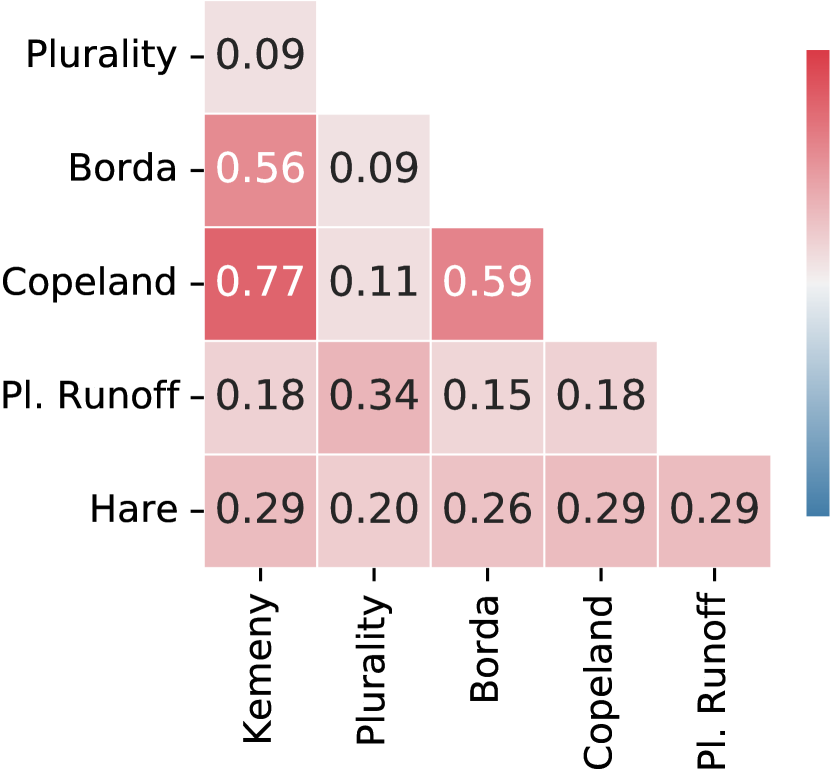
(a) All elections.

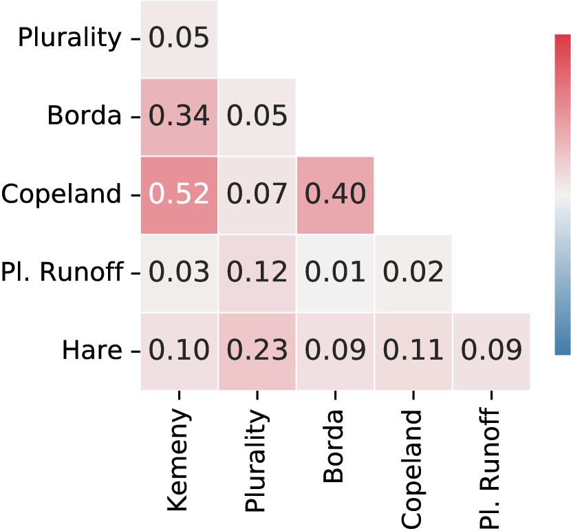
(b) All elections not admitting a Condorcet winner.

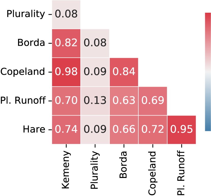
(c) All boxing top 16 elections.

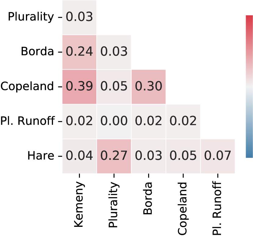
(d) All city rankings elections.

Figure 11: Average Spearman’s rank correlation coefficient of different pairs of voting rules on different datasets.

On the dataset level, results again vary substantially. In Figure 11(c), we show the average Spearman coefficient for boxing top 16 elections where the consensus is the highest, while in Figure 11(d) we depict the average Spearman coefficient for city rankings where the consensus is the lowest. In the boxing top 16 dataset, all rules (except for Plurality which has a very low correlation with all other rules) have a pairwise average Spearman coefficient of at least $0.63$, especially Copeland and Kemeny (with $0.98$) and Hare and Plurality with Runoff ($0.95$) are highly correlated. However, given that Plurality and Plurality with runoff work quite similar, their lack of correlation is quite surprising. Turning to city ranking elections, most of the rules produce completely uncorrelated rankings. Only Copeland, Borda and Kemeny together with Plurality and Hare still have some noticeable, yet still quite low, correlation.

8 Conclusion

We have collected, classified, analyzed, and used a diverse collection of real-world elections and provided various evidence hinting at their usefulness for experimental research. To the best of our knowledge, this is the first work that systematically compares elections from numerous different sources.

For future work, it would be interesting to analyze the relationship of the collected elections to elections drawn from various statistical cultures. Moreover, also performing our experiments on such synthetic elections could be useful to get a better understanding of their properties. In addition, examining the collected elections (even) more carefully would be of great use: While we have been able to provide intuitive explanations for some phenomena we observed, the reasons for others remain unclear. Furthermore, as we have found only little evidence to support the large-scale practical applicability of already developed parameterized algorithms, identifying new properties that are shared by many elections and that allow for the development of tractable algorithms would be extremely valuable. Finally, the main purpose of this project is to provide a helpful source of real-world election datasets, so we hope that others will find our data useful in bridging the gap between theory and practice in computational social choice.

Acknowledgments

NB was supported by the DFG project MaMu (NI 369/19) and by the DFG project ComSoc-MPMS (NI 369/22). NS was supported by the DFG project MaMu (NI 369/19). The authors would like to thank Piotr Faliszewski for constructive criticism of the manuscript.

name	type	raw				relevant complete
		#Elec.	Avg. #Voters	Avg. #Cand.		#Elec.	Avg. #Voters	Avg. #Cand.
board games	time	1	130	5904		1	130	885
table tennis top	time	38	11.32	1429.92		36	11.5	670.47
Giro d’Italia	time	99	19.27	102.2		23	16.83	130.13
marblelympics	time	5	13.4	19.4		4	12.25	15.75
mylaps	time	635	28.67	25.87		394	25.33	29.59
football combined	crit.	23	1466.26	228.48		23	506.39	217.87
basketball season	time	1095	13.54	325.06		966	14.19	336.42
basketball week	crit.	382	38.82	342.38		378	35.8	337.34
basketball combined	crit.	20	741.5	341.65		20	671.4	315.65
baseball season	time	174	12.74	217.99		127	12.24	263.98
baseball week	crit.	159	14.3	299.47		158	10.34	192.44
baseball combined	crit.	10	221.6	299.8		10	134.8	249.6

Table 3: Information about not-used election datasets.

Appendix A Additional Material for Section 3

A.1 Further Datasets

In the following, we present the additional datasets that we created. Notably, we could have also included all of them in our analysis from the main body but decided against it for the sake of conciseness. In Table 3, we present basic information about our further non-used datasets analgous to Table 1.

Board Games.

The board games data (collected by Snow [74]) contains a weekly ranking of the 2000 most popular board games on boardgamegeek.com between October 2018 and December 2021. We created a single board games election where each game is a candidate and each vote corresponds to the ranking of the games in one week.

Table Tennis (World) Rankings.

The table tennis data (collected by Zydyk [87]) contains the monthly ITTF ranking of the top 500-1500 male and female table tennis players between 2001 and 2020. For each year, we created a table tennis election where each player is a candidate and each vote corresponds to the ranking of the players in one month.

Giro d’Italia.

For each edition of the Giro d’Italia between 1910 and 2020, the data contains the completion times of all riders for each stage of the edition. The dataset was crawled by us from the website procyclingstats.com. For each edition, we created one Giro d’Italia election in which the riders are the candidates and each vote corresponds to a stage and ranks the riders by their completion time.

Marblelympics.

The marblelympics are a competition of marbles in multiple races broadcasted on youtube.com. For each edition of the marblelympics between 2016 and 2020, the data contains the completion times of all marbles for each stage of the edition. The dataset was crawled by us from the website jellesmarbleruns.fandom.com. For each edition, we created one marblelympics election in which the marbles are the candidates and each vote corresponds to a race and ranks the marbles by their completion time.

Mylaps.

The mylaps data contains the completion time of athletes in each lap of a multi-lap competition (specifically, speed skating and cycling competitions). The dataset was crawled by us from the website http://results.sporthive.com/. For each race, we created one mylaps election in which the athletes are the candidates and each vote corresponds to one lap and ranks the athletes by their completion time.

College Sports.

Apart from the American football data presented and used in the main body, the college sports data (collected by Massey [51]) also contains weekly power rankings of college basketball teams (between 2001 and 2021) and college baseball teams (between 2010 and 2021) from different media outlets and ranking systems. For all three data sources, we created three different types of elections with teams as candidates: First, for each season and each ranking system, we created a season election where each vote corresponds to the power ranking of the teams in one week according to the ranking system. Second, for each week in one of the seasons, we created a week election where each vote corresponds to the power ranking of the teams in this week according to one of the ranking systems. Third, for each season, we created a combined election where each vote corresponds to the power ranking of the teams in one of the weeks according to one of the ranking systems.

Appendix B Additional Material for Section 6

B.1 Properties of Elections From or Close to a Restricted Domain

• Elections from a restricted domain are typically quite degenerate.

• In single-peaked elections the top-choices of all voters typically come from the same part of the societal order.

• Single-peaked or single-crossing elections that arise from deleting some candidates or voters from our election are more diverse than initially single-peaked or single-crossing elections.

Given that all but two of our elections that are part of a restricted domain come from the boxing top 16 dataset which contains elections where votes are typically very similar to each other, in this section we want to analyze the structural properties of elections that are part of or close to a restricted domain. In particular, we are interested in whether these elections are simply “degenerate“ (with all voters having more or less the same preferences, thereby being part of a restricted domain more “by accident” than “by design”) or “exploit” the full space of the domain (recall that, for instance, an election where half of the voters rank the candidates in one order and the other rank them in the opposite order is single-peaked, single-crossing, and group-separable).

B.1.1 Elections from a Restricted Domain

We first consider elections that are part of a restricted domain and show in Figure 12 a cumulative plot of their Kemeny score: A large majority of elections from a restricted domain have a Kemeny score below $100$, while only around $6\%$ of all elections have a Kemeny score below $100$. In single-peaked elections, votes are especially similar ($86\%$ have a Kemeny score below $50$), whereas for single-crossingness there are at least $22$ elections ($16\%$) with a Kemeny score above $100$. Nevertheless, it seems that in real-world elections from a restricted domain voters have very similar preferences and that these elections only cover a very small part of the space of all elections from this restricted domain.

Figure 12: Fraction of single-peaked (blue), single-crossing (orange), group-separable (green), and all elections (red) whose Kemeny score is at most the value displayed on the $x$-axis.

Figure 13: Average Kemeny score of elections within a given candidate deletion distance to single-peakedness (blue), single-crossingness (orange), or group-separability (green).

Figure 14: Number of elections (y-axis) with a given number of top-choices (x-axis).

Considering all elections, there is a clear connection between the Kemeny score of an election and its distance to a restricted domain: In Figure 14, for each restricted domain, we depict the average Kemeny score of elections within some candidate deletion distance. The plot clearly shows that the further an election is away from a restricted domain, the higher, on average, is its Kemeny score. While for smaller candidate deletion distances, the average Kemeny score roughly increases by $30$ if we increase the distance by one, there is a rapid increase by roughly $200$ when moving from distance $10$ to $11$ (notably, for each restricted domain, roughly $30\%$ of all elections are at candidate deletion distance $11$). For the voter deletion distance the picture is similar. Overall, these findings indicate that in elections from or close to a restricted domain votes are similar to each other.

(a) candidate deletion

(b) voter deletion

Figure 15: In solid (dotted), number of different top-choices of voters for elections at a certain distance from single-peakedness after (before) deleting the respective candidates or voters.

(a) All of our elections which are single-peaked.

(b) All of our elections which are single-peaked after applying a random tie-breaking when computing a compatible societal order.

(c) Single-peaked elections obtained from deleting $3$ candidates from elections at candidate deletion distance $3$.

(d) Single-peaked elections obtained from deleting $12$ voters from elections at voter deletion distance $12$.

(e) Single-peaked elections obtained from deleting $25$ voters from elections at voter deletion distance $25$.

Figure 16: Each single-peaked election comes with a societal order. The diagrams depict where the top-choices of voters lie on this axis. Specifically, for each $i\in[15]$, we depict the number of voters that have the $i$th candidate from the societal order as their top-choice for different types of single-peaked elections.

B.1.2 (Close to) Single-Peakedness

For single-peaked elections a very simple measure for how degenerate elections are is the number of different top-choices of voters, as the top-choice of a voter in a single-peaked election fundamentally influences the vote and in principle all top-choices are possible. To get a feeling for how many different top-choices an election typically has, in Figure 14, we depict the distribution of the number of different top-choices in an election. On average, our elections have only $4.081$ different top-choices.

Number of Different Top-Choices.

Out of our $79$ single-peaked elections, in $78$ of them, all voters have the same top-choice and in only one of them, voters have two different ones. This indicates again the degenerateness of the found single-peaked elections. Moreover, in Figure 15, in dotted lines we depict the average number of different top-choices in elections at a given voter and candidate deletion distance. Remarkably, for elections up to candidate deletion distance $6$ and up to voter deletion distance $19$ the average number of top-choices is smaller than $2$ and only moving (even) further away from single-peakedness leads to a substantial increase in the number of top-choices. This suggests that also elections close to single-peakedness do not capture the full space of these elections. However, it is also possible to take a different view here and to consider the elections at some distance to single-peakedness after the deletion of candidates or voters (so the elections that remain and that are actually single-peaked). The results are depicted in the solid lines in Figure 15. Interestingly, the elections created this way seem to be a bit more diverse than originally single-peaked elections: Until candidate deletion distance $11$ the average number of top-choices constantly increases from around $1.5$ top-choices at distance $3$ to around $3$ top-choices at distance $11$. For the voter deletion distance we have a more or less constant increase from around $1$ for distance $0$ to around $1.7$ for distance $27$. This steady increase is even more remarkable considering that by deleting voters or candidates we decrease the maximum number of possible different top-choices.

Interestingly, the results from the previous paragraph suggest that the Walsh model [80] to sample single-peaked preferences might be more realistic than the Conitzer model [19]. In the Walsh model, one samples an election from the space of single-peaked elections uniformly at random and with a high-probability the top choice of all voters is one of the middle (two) candidates from the societal order. In contrast to this, in the Conitzer model, top-choices of voters are drawn uniformly at random. This hypothesis gets confirmed in the next paragraph.

Position of Top-Choices in the Societal Order.

Next, we analyze where top-choices of voters in single-peaked elections lie on the societal order. Without loss of generality assume that the societal order is $c_{1}\succ\dots\succ c_{15}$ (if this is not the case we can relabel the candidates). Thus, $c_{1}$ and $c_{15}$ are the extreme candidates in this election (e.g., in case that an election models a political election these could be the left extremist and right extremists candidates), whereas $c_{7}$ and $c_{8}$ are in some sense the center candidates. We are now interested in the rank of the top-choice of each voter in the societal order, which corresponds to the candidate’s index for the societal order $c_{1}\succ\dots\succ c_{15}$. For this, we look at the single-peaked elections that are obtained from our initial elections by deleting a minimum number of candidates or voters (i.e., the single-peaked “cores” of our elections obtained when computing the respective distances to single-peakedness). We depict the frequency of top-choice ranks in the societal order in Figure 16. In Figure 16(a), we consider all elections from our dataset which are single-peaked. The results are remarkable in two ways.

First, the top-choices of voters do not lie in the middle of the societal order (like one would probably intuitively expect it), but are heavily skewered to one side. One explanation for this could be the single-peaked detection algorithm by Escoffier et al. [32] which we use. This algorithm constructs the societal order in a greedy fashion by successively inserting candidates ranked last by some voter at the extremes of the societal order. Ties are here broken always by inserting candidates on the top free position in the societal order, which could result in top-choices of voters typically being inserted rather in the bottom of the axis. To check this hypothesis, we reran the experiments with an adapted variant of the single-peaked detection algorithm, where we break ties independent uniformly at random and depict the results in Figure 16(b). Indeed, the top-choices of voters now lie in the middle of the axis. Consequently, the voters top-choices are not “truly” skewered to one side. Nevertheless, these observations still allow for some non-obvious conclusions concerning our data: Single-peaked elections are typically consistent with many potentially quite different axes, indicating that the final axis carries only little meaning and in single-peaked elections votes are quite similar.

Second, the top-choices of voters come all more or less from the same part of the societal order. Remarkably, there is not a single vote in all single-peaked elections where one of the first eight candidates from the societal order is ranked in the first position. In principle, any distribution is possible. For instance, the synthetic Conitzer model assumes a uniform distribution of top-choice ranks. This seems to be far away from reality. However, this might be also due to to fact that all but two of our single-peaked elections come from the boxing top 16 dataset in which votes are anyway quite similar. Thus, to test this observation we now also look at the single-peaked elections that result from deleting a minimum number of voters or candidates from close to single-peaked elections.

We start by looking at the single-peaked elections that result from deleting $i$ candidates from elections that are at candidate deletion distance $i$ from being single-peaked. We depict the corresponding plot for $i=3$ in Figure 16(c). Independent of the value $i$, the plots always look similar to a Gaussian distribution, confirming our earlier observation that all voters typically have top-choices from the same part of the societal order. However, for increasing $i$ the peak of the distribution moves towards the center of the societal order. For instance, after removing for instance $3$ candidates, the most frequent top-choice rank is $7$. This indicates that the generated elections are no longer compatible with a lot of quite different societal orders.

If we instead consider single-peaked elections that result from deleting $i$ voters from elections that are at voter deletion distance $i$ from being single-peaked, the picture is slightly different: Here, for $i\in[0,22]$, the distribution is again similar to a Gaussian distribution with the peak slowly shifting towards the center. We depict the distribution for $i=12$ in Figure 16(d). However, for $i\geq 23$, more and more votes start to have the last candidate from the societal order as their top choice (see Figure 16(e) for $i=25$ for an example). Note that if a voter has the last candidate from the axis as its top-choice, then its vote is already fully determined by this (as the reversed societal order). This indicates that in elections at a large voter deletion distance the single-peaked core simply consists of identical votes.

B.1.3 (Close to) Single-Crossingness

Recall that for single-crossingness we require that if we move along the central order of voters the ordering of each pair of candidates changes at most once. So the extremely diverse case would be that each pair of candidates changes ordering exactly once. This is why we consider the fraction of pairs of candidates that change their ordering as a measure for the degenerateness of the election. Here for candidate/voter deletion distance larger than zero, we analyze only the properties of the elections that remain after the deletion of candidates or voters (as for the original elections there is no ordering of voters).

In Figure 17, we show the results. While for single-crossing elections only on average $6.5\%$ of candidate pairs swap their ordering when moving along the central order, for increasing candidate deletion distance this value constantly increases until almost all of the remaining candidate pairs switch their ordering. For increasing voter deletion distance it increases until half of all candidate pairs switch their ordering. The difference between the behavior for the candidate and voter deletion distance here is probably due to the fact that with fewer candidates remaining it becomes “easier” to swap the ordering of all candidate pairs, while with fewer voters remaining it becomes in some sense “harder”. Nevertheless, the results also suggest here that the single-crossing “core” of non-single-crossing elections is much more diverse than full single-crossing elections from our dataset.

(a) candidate deletion

(b) voter deletion

Figure 17: Fraction of candidate pairs who are not ranked in the same order by all voters for elections at a certain distance from single-crossingness after deleting the respective candidates or voters.

B.2 General Preference Restrictions

All three considered restricted domains can be characterized via two forbidden configurations (meaning that elections are part of the domain if they do not contain both forbidden configurations). The most important configurations are:

$\boldsymbol{\alpha}$-configuration

: Two voters $v$ and $v^{\prime}$ and four candidates $a,b,c$, and $d$ with:

$$a\succ b\succ c\wedge d\succ b\text{ and }c\succ^{\prime}b\succ^{\prime}a\wedge d\succ^{\prime}b.$$

$\boldsymbol{\beta}$-configuration

: Two voters $v$ and $v^{\prime}$ and four candidates $a,b,c,$ and $d$ with:

$$a\succ b\succ c\succ d\text{ and }b\succ^{\prime}d\succ^{\prime}a\succ^{\prime}c.$$

$\boldsymbol{\gamma}$-configuration

: Three voters $v$, $v^{\prime}$, and $v^{\prime\prime}$ and six (possibly identical) candidates $a,b,c,d,e,$ and $f$ with:

$$b\succ a\wedge c\succ d\wedge e\succ f\text{ and }$$

$$a\succ^{\prime}b\wedge d\succ^{\prime}c\wedge e\succ^{\prime}f\text{ and }$$

$$a\succ^{\prime\prime}b\wedge c\succ^{\prime\prime}d\wedge f\succ^{\prime\prime}e.$$

$\boldsymbol{\delta}$-configuration

: Four voters $v$, $v^{\prime}$, $v^{\prime\prime}$, and $v^{\prime\prime\prime}$ and four (possibly identical) candidates $a,b,c,$ and $d$ with:

$$a\succ b\wedge c\succ d\text{ and }$$

$$a\succ^{\prime}b\wedge d\succ^{\prime}c\text{ and }$$

$$b\succ^{\prime\prime}a\wedge c\succ^{\prime\prime}d\text{ and }$$

$$b\succ^{\prime\prime\prime}a\wedge d\succ^{\prime\prime\prime}c.$$

best-configuration

Three voters $v$, $v^{\prime}$, and $v^{\prime\prime}$ and three candidates $a,b,$ and $c$ with:

$$a\succ b\wedge a\succ c\text{ and }b\succ^{\prime}a\wedge b\succ^{\prime}c\text{ and }c\succ^{\prime\prime}a\wedge c\succ^{\prime\prime}b.$$

worst-configuration

Three voters $v$, $v^{\prime}$, and $v^{\prime\prime}$ and three candidates $a,b,$ and $c$ with:

$$a\succ c\wedge b\succ c\text{ and }a\succ^{\prime}b\wedge c\succ^{\prime}b\text{ and }b\succ^{\prime\prime}a\wedge c\succ^{\prime\prime}a.$$

medium-configuration

Three voters $v$, $v^{\prime}$, and $v^{\prime\prime}$ and three candidates $a,b,$ and $c$ with:

$$b\succ a\succ c\vee c\succ a\succ b\text{ and }$$

$$a\succ^{\prime}b\succ^{\prime}c\vee c\succ^{\prime}b\succ^{\prime}a\text{ and }$$

$$a\succ^{\prime\prime}c\succ^{\prime\prime}b\vee b\succ^{\prime\prime}c\succ^{\prime\prime}a.$$

value-configuration

Three voters $v$, $v^{\prime}$, and $v^{\prime\prime}$ and three candidates $a,b,$ and $c$ with:

$$a\succ b\succ c\text{ and }b\succ^{\prime}c\succ^{\prime}a\text{ and }c\succ^{\prime\prime}a\succ^{\prime\prime}b.$$

The domains of best/worst/medium/value-restricted elections are characterized by the absence of best/worst/medium/value-configurations. Elections without a best-, worst-, or medium-configuration also do not admit a value-configuration.

Single-peaked elections are characterized by the absence of $\alpha$- and worst-configurations. Single-crossing elections are characterized by the absence of $\gamma$- and $\delta$-configurations. Group-separable elections are characterized by the absence of $\beta$- and medium-configurations.

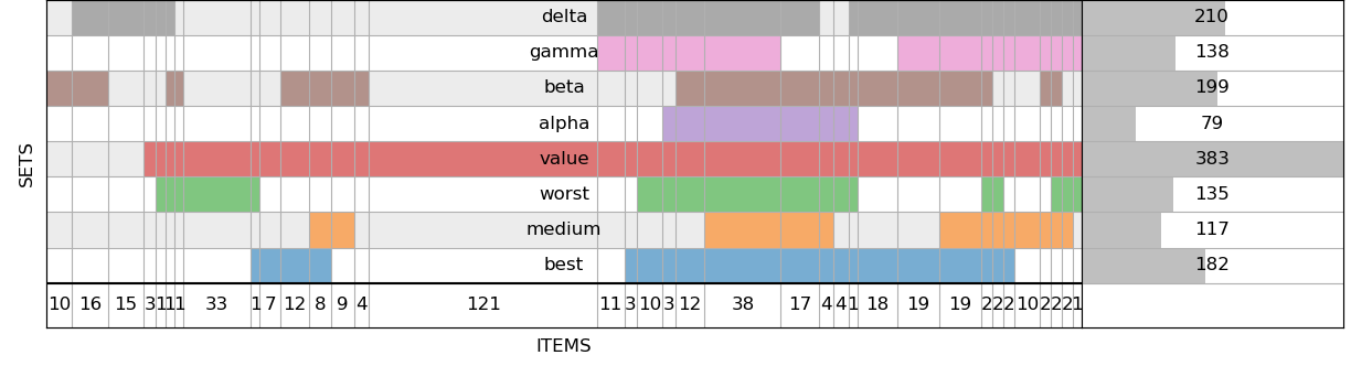
Figure 18: Diagram visualization the number of elections which do not admit a forbidden configuration. Each line corresponds to one configuration. For each configuration, in the right most column, the number of elections without the respective configuration is shown. In the other columns elections that do not admit one or multiple configurations are represented: Their number can be found at the bottom and the configurations they do not contain are highlighted. For instance, the second column says that there are $16$ elections that do not admit a $\beta$- and $\delta$- configuration.

In Figure 18, we visualize the number and relationship of elections that do not admit one (or multiple) of the forbidden configurations. We find that for single-peaked elections, which are characterized by the absence of $\alpha$- and worst-configurations, worst-configurations are practically irrelevant as all elections that do not admit a $\alpha$-configuration also do not admit a worst-configuration. Similarly, for single-crossing elections (characterized by the absence of $\gamma$- and $\delta$-configurations) $\delta$-configurations are fully redundant. For group-separable elections (characterized by the absence of $\beta$- and medium-configurations) $\beta$-configurations are redundant in most cases. Lastly, there is one configuration which in an overwhelming majority of elections does not appear if any other configuration does not appear (some of these relationships are theoretically guaranteed): value-configurations. Among the $424$ elections not admitting one of the forbidden configurations, $383$ do not admit a value-configuration. This hints at the practical relevance of value-restricted elections [70] as a (more) frequently occurring restricted domain.

Motivated by this observation, we also checked the voter deletion and candidate deletion of our elections from being value-restricted using the algorithmic ideas of Elkind and Lackner [25]. In Figure 19 we depict a cumulative distribution function visualization the fraction of elections that are within a certain candidate/voter deletion distance from single-peaked/single-crossing/group-seperable/value-restricted (note that this figure is the same as Figure 7 but with added black lines for value-restricted). As visible in Figure 19(a), while elections are in fact closer to being value-restricted than to any of the other three restricted domains, there are still only few elections within a small voter/candidate deletion distance. The difference between value-restrictedness and the other three restricted domains is most pronounced for the voter deletion distance for spotify month elections (Figure 19(a)): Here, usually around $10$ less voters need to be deleted to make an election value restricted than to make it fall into one of the other three restricted domains. The other datasets from our first group close to identity exhibit a similar behavior.

(a) aggregated

(b) spotify month

Figure 19: Fraction of elections within a given candidate deletion (solid) or voter deletion distance (dashed) from single-peakedness (blue), single-crossingness (orange), group-separability (green), and value-restricted (black).

Appendix C Additional Material for Section 7

C.1 Number of Ties and Impact on Winner Consensus

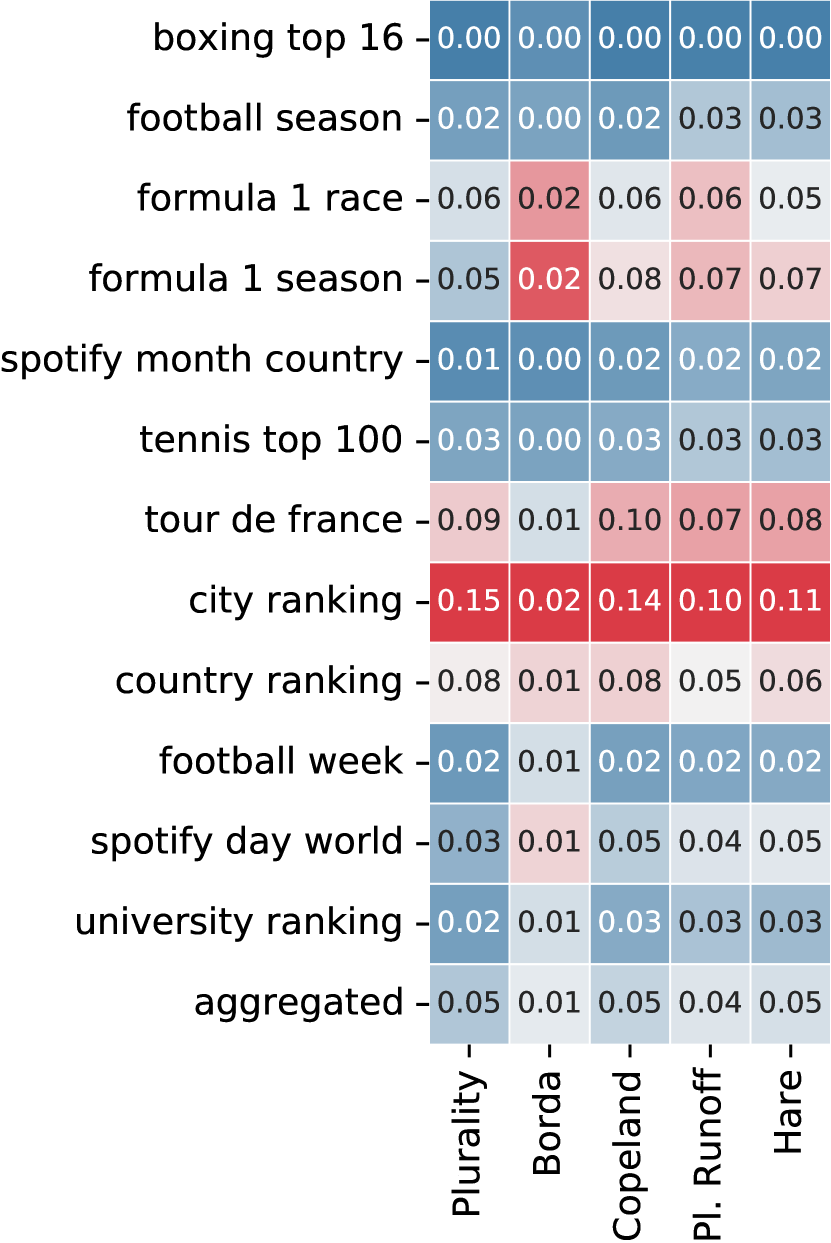
(a) All elections.

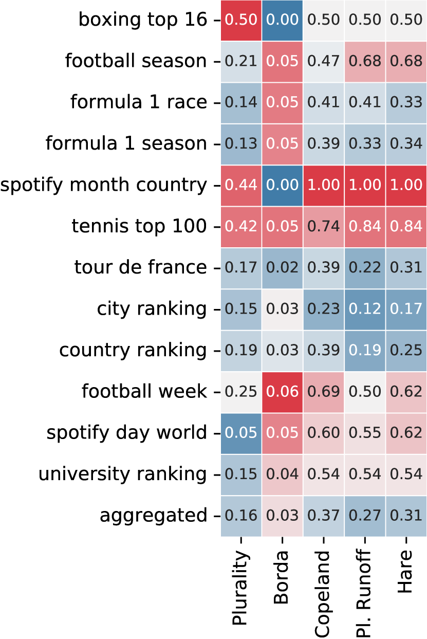
(b) Elections without strong Condorcet winner

Figure 20: Fraction of elections where voting rules returned multiple winners. Colors express normalized values which are normalized with respect to the maximum in each column.

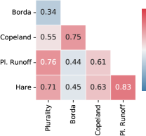
Figure 21: Non-empty overlap on all elections without Condorcet winner.

We computed three different ways of evaluating the similarity of winners returned by different voting rules:

Lexicographic agreement

This measure is one if in case that we apply lexicographic tie-breaking, the returned winner is the same and zero otherwise.

Non-empty overlap

This measure is one if the winner sets overlap and zero otherwise.

Normalized overlap

For two winner sets $W_{1}$ and $W_{2}$ of two voting rules the overlap is $\nicefrac{{|W_{1}\cap W_{2}|}}{{|W_{1}\cup W_{2}|}}$.

Note that these three measures coincide if both voting rules return a unique winner. So let us focus for a moment on how often the considered voting rules select more than one winner. As shown in Figure 20(a), all our voting rules expect Borda return a tied winner on only $5\%$ of all elections; for Borda it is only $1\%$ of elections. One possible explanation for this could be that most of our elections admit a strong Condorcet winner and that in this case rules are likely to return it as the unique winner. Examining Figure 20(b), where we depict the fraction of elections without a strong Condorcet winner that are tied, this intuition gets confirmed: Under all voting rules, the fraction of all elections without a strong Condorcet winner that are tied is at least three times higher than for all elections. That is, of all elections without a strong Condorcet winner $16\%$, $3\%$, $37\%$, $27\%$, and $31\%$ are tied under Plurality, Borda, Copeland, Plurality with Runoff and Hare, respectively. In particular, for Copeland, Plurality with Runoff and Hare are these values remarkably high. This might be due to the fact that all these three voting rules might boil down to a pairwise comparison between two candidates: While a strong Condorcet winner always wins such a comparison, without one ties can arise. Lastly, observe that as the fraction of elections with a strong Condorcet winner varies significantly among our datasets, it is quite intuitive that the fraction of tied elections also depends on the dataset.

Coming back to our original question of comparing our three measures for the consensus of voting rules, lexicographic agreement and normalized overlap produce mostly very similar results. For lexicographic agreement and non-empty overlap, results are similar for the aggregate dataset but differ slightly more on elections without strong Condorcet winners (which is also quite intuitive because we previously observed that these elections are more likely to be tied). In Figure 21, we display the average non-empty overlap for elections without a strong Condorcet winner (for the aggregate dataset the picture for non-empty overlap is very similar to the one for lexicographic agreement). As the non-empty overlap measure is always one if the lexicographic agreement is one, comparing Figure 21 to the analgous plot (Figure 10(b)) for the lexicographic agreement, we observe that the values for the non-empty overlap are higher. However, given that we previously observed that voting rules return tied winners only on a minority of elections, the extent (e.g., for Hare and Plurality the lexicographic agreement is $0.5$ and the non-empty overlap is $0.71$) is partly surprising. Moreover, the results for the non-empty overlap confirm our proposed splitting of voting rules into two groups.

References

- Baumeister et al. [2020] D. Baumeister, T. Hogrebe, and J. Rothe. Towards reality: Smoothed analysis in computational social choice. In Proceedings of the 19th International Conference on Autonomous Agents and Multiagent Systems (AAMAS ’20), pages 1691–1695. IFAAMAS, 2020.
- Betzler et al. [2009] N. Betzler, M. R. Fellows, J. Guo, R. Niedermeier, and F. A. Rosamond. Fixed-parameter algorithms for kemeny rankings. Theor. Comput. Sci., 410(45):4554–4570, 2009.
- Betzler et al. [2013] N. Betzler, A. Slinko, and J. Uhlmann. On the computation of fully proportional representation. J. Artif. Intell. Res., 47:475–519, 2013.
- Betzler et al. [2014] N. Betzler, R. Bredereck, and R. Niedermeier. Theoretical and empirical evaluation of data reduction for exact kemeny rank aggregation. Auton. Agents Multi Agent Syst., 28(5):721–748, 2014.
- Black [1948] D. Black. On the rationale of group decision-making. J. Polit. Econ., 56(1):23–34, 1948.
- Blitzer [2017] Blitzer. Movehub city rankings, 2017. kaggle.com/blitzr/movehub-city-rankings. Data obtained from movehub.com.
- Boehmer and Niedermeier [2021] N. Boehmer and R. Niedermeier. Broadening the research agenda for computational social choice: Multiple preference profiles and multiple solutions. In Proceedings of the 20th International Conference on Autonomous Agents and Multiagent Systems (AAMAS ’21), pages 1–5. ACM, 2021.
- Boehmer et al. [2021a] N. Boehmer, R. Bredereck, P. Faliszewski, and R. Niedermeier. Winner robustness via swap- and shift-bribery: Parameterized counting complexity and experiments. In Proceedings of the Thirtieth International Joint Conference on Artificial Intelligence (IJCAI ’21), pages 52–58. ijcai.org, 2021a.
- Boehmer et al. [2021b] N. Boehmer, R. Bredereck, P. Faliszewski, R. Niedermeier, and S. Szufa. Putting a compass on the map of elections. In Proceedings of the Thirtieth International Joint Conference on Artificial Intelligence (IJCAI ’21), pages 59–65. ijcai.org, 2021b.
- Boehmer et al. [2021c] N. Boehmer, R. Bredereck, P. Faliszewski, R. Niedermeier, and S. Szufa. Putting a compass on the map of elections. CoRR, abs/2105.07815, 2021c. URL https://arxiv.org/abs/2105.07815.
- Brandt et al. [2015] F. Brandt, M. Brill, E. Hemaspaandra, and L. A. Hemaspaandra. Bypassing combinatorial protections: Polynomial-time algorithms for single-peaked electorates. J. Artif. Intell. Res., 53:439–496, 2015.
- Brandt et al. [2016a] F. Brandt, V. Conitzer, U. Endriss, J. Lang, and A. D. Procaccia, editors. Handbook of Computational Social Choice. Cambridge University Press, 2016a.
- Brandt et al. [2016b] F. Brandt, C. Geist, and M. Strobel. Analyzing the practical relevance of voting paradoxes via ehrhart theory, computer simulations, and empirical data. In Proceedings of the 2016 International Conference on Autonomous Agents & Multiagent Systems (AAMAS ’16), pages 385–393. ACM, 2016b.
- Bredereck et al. [2016] R. Bredereck, J. Chen, and G. J. Woeginger. Are there any nicely structured preference profiles nearby? Math. Soc. Sci., 79:61–73, 2016.
- Bredereck et al. [2019] R. Bredereck, P. Faliszewski, A. Kaczmarczyk, and R. Niedermeier. An experimental view on committees providing justified representation. In Proceedings of the Twenty-Eighth International Joint Conference on Artificial Intelligence (IJCAI ’19), pages 109–115. ijcai.org, 2019.
- Bredereck et al. [2020] R. Bredereck, T. Fluschnik, and A. Kaczmarczyk. Multistage committee election. CoRR, abs/2005.02300, 2020. URL https://arxiv.org/abs/2005.02300.
- Caragiannis et al. [2016] I. Caragiannis, E. Hemaspaandra, and L. A. Hemaspaandra. Dodgson’s rule and young’s rule. In F. Brandt, V. Conitzer, U. Endriss, J. Lang, and A. D. Procaccia, editors, Handbook of Computational Social Choice, pages 103–126. Cambridge University Press, 2016.
- Chamberlin et al. [1984] J. R. Chamberlin, J. L. Cohen, and C. H. Coombs. Social choice observed: Five presidential elections of the american psychological association. J. Polit., 46(2):479–502, 1984.
- Conitzer [2009] V. Conitzer. Eliciting single-peaked preferences using comparison queries. J. Artif. Intell. Res., 35:161–191, 2009.
- Conitzer and Sandholm [2006] V. Conitzer and T. Sandholm. Nonexistence of voting rules that are usually hard to manipulate. In Proceedings of the Twenty-First National Conference on Artificial Intelligence (AAAI ’06), pages 627–634. AAAI Press, 2006.
- Conitzer and Walsh [2016] V. Conitzer and T. Walsh. Barriers to manipulation in voting. In F. Brandt, V. Conitzer, U. Endriss, J. Lang, and A. D. Procaccia, editors, Handbook of Computational Social Choice, pages 127–145. Cambridge University Press, 2016.
- Cornaz et al. [2013] D. Cornaz, L. Galand, and O. Spanjaard. Kemeny elections with bounded single-peaked or single-crossing width. In Proceedings of the 23rd International Joint Conference on Artificial Intelligence (IJCAI ’13), pages 76–82. IJCAI/AAAI, 2013.
- Darmann et al. [2019] A. Darmann, J. Grundner, and C. Klamler. Evaluative voting or classical voting rules: Does it make a difference? empirical evidence for consensus among voting rules. Eur. J. Polit. Econ., 59:345–353, 2019.
- Doucette [2014] J. A. Doucette. Imputation, social choice, and partial preferences. In Proceedings of the Twenty-Eighth AAAI Conference on Artificial Intelligence (AAAI ’14), pages 3069–3070. AAAI Press, 2014.
- Elkind and Lackner [2014] E. Elkind and M. Lackner. On detecting nearly structured preference profiles. In Proceedings of the Twenty-Eighth AAAI Conference on Artificial Intelligence (AAAI ’14), pages 661–667. AAAI Press, 2014.
- Elkind et al. [2012] E. Elkind, P. Faliszewski, and A. M. Slinko. Clone structures in voters’ preferences. In Proceedings of the 13th ACM Conference on Electronic Commerce (EC ’12), pages 496–513. ACM, 2012.
- Elkind et al. [2016a] E. Elkind, M. Lackner, and D. Peters. Preference restrictions in computational social choice: Recent progress. In Proceedings of the Twenty-Fifth International Joint Conference on Artificial Intelligence (IJCAI ’16), pages 4062–4065. IJCAI/AAAI Press, 2016a.
- Elkind et al. [2016b] E. Elkind, E. Markakis, S. Obraztsova, and P. Skowron. Complexity of finding equilibria of plurality voting under structured preferences. In Proceedings of the 2016 International Conference on Autonomous Agents & Multiagent Systems (AAMAS ’16), pages 394–401. ACM, 2016b.
- Elkind et al. [2017] E. Elkind, M. Lackner, and D. Peters. Structured preferences. In U. Endriss, editor, Trends in Computational Social Choice, chapter 10, pages 187–208. AI Access, 2017.
- Elkind et al. [2020] E. Elkind, P. Faliszewski, and P. Skowron. A characterization of the single-peaked single-crossing domain. Soc. Choice Welf., 54(1):167–181, 2020.
- Erdélyi et al. [2017] G. Erdélyi, M. Lackner, and A. Pfandler. Computational aspects of nearly single-peaked electorates. J. Artif. Intell. Res., 58:297–337, 2017.
- Escoffier et al. [2008] B. Escoffier, J. Lang, and M. Öztürk. Single-peaked consistency and its complexity. In Proceedings of the 18th European Conference on Artificial Intelligence (ECAI ’08), pages 366–370. IOS Press, 2008.
- Faliszewski and Rothe [2016] P. Faliszewski and J. Rothe. Control and bribery in voting. In F. Brandt, V. Conitzer, U. Endriss, J. Lang, and A. D. Procaccia, editors, Handbook of Computational Social Choice, pages 146–168. Cambridge University Press, 2016.
- Faliszewski et al. [2011] P. Faliszewski, E. Hemaspaandra, L. A. Hemaspaandra, and J. Rothe. The shield that never was: Societies with single-peaked preferences are more open to manipulation and control. Inf. Comput., 209(2):89–107, 2011.
- Faliszewski et al. [2014] P. Faliszewski, E. Hemaspaandra, and L. A. Hemaspaandra. The complexity of manipulative attacks in nearly single-peaked electorates. Artif. Intell., 207:69–99, 2014.
- Faliszewski et al. [2018a] P. Faliszewski, M. Lackner, D. Peters, and N. Talmon. Effective heuristics for committee scoring rules. In Proceedings of the Thirty-Second AAAI Conference on Artificial Intelligence, (AAAI ’18), pages 1023–1030. AAAI Press, 2018a.
- Faliszewski et al. [2018b] P. Faliszewski, A. Slinko, K. Stahl, and N. Talmon. Achieving fully proportional representation by clustering voters. J. Heuristics, 24(5):725–756, 2018b.
- Faliszewski et al. [2020] P. Faliszewski, A. Karpov, and S. Obraztsova. The complexity of election problems with group-separable preferences. In Proceedings of the Twenty-Ninth International Joint Conference on Artificial Intelligence (IJCAI ’20), pages 203–209. ijcai.org, 2020.
- Felsenthal et al. [1993] D. S. Felsenthal, Z. Maoz, and A. Rapoport. An empirical evaluation of six voting procedures: do they really make any difference? Br. J. Polit. Sci., 23(1):1–27, 1993.
- Fruchterman and Reingold [1991] T. Fruchterman and E. Reingold. Graph drawing by force-directed placement. Software Pract. Exper., 21(11):1129–1164, 1991.
- Goldsmith et al. [2014] J. Goldsmith, J. Lang, N. Mattei, and P. Perny. Voting with rank dependent scoring rules. In Proceedings of the Twenty-Eighth AAAI Conference on Artificial Intelligence (AAAI ’14), pages 698–704. AAAI Press, 2014.
- Gurobi Optimization, LLC [2021] Gurobi Optimization, LLC. Gurobi Optimizer Reference Manual. https://www.gurobi.com, 2021.
- Inada [1964] K.-i. Inada. A note on the simple majority decision rule. Econometrica, pages 525–531, 1964.
- Inada [1969] K.-i. Inada. The simple majority decision rule. Econometrica, pages 490–506, 1969.
- Jürisoo [2021] M. Jürisoo. Ufc rankings, 2021. kaggle.com/martj42/ufc-rankings. Data obtained from ufc.com.
- Keller et al. [2019] O. Keller, A. Hassidim, and N. Hazon. New approximations for coalitional manipulation in scoring rules. J. Artif. Intell. Res., 64:109–145, 2019.
- Lackner [2020] M. Lackner. Perpetual voting: Fairness in long-term decision making. In Proceedings of the Thirty-Fourth AAAI Conference on Artificial Intelligence (AAAI ’20), pages 2103–2110. AAAI Press, 2020.
- Lang and Xia [2016] J. Lang and L. Xia. Voting in combinatorial domains. In F. Brandt, V. Conitzer, U. Endriss, J. Lang, and A. D. Procaccia, editors, Handbook of Computational Social Choice, pages 197–222. Cambridge University Press, 2016.
- Lonardi et al. [2006] S. Lonardi, W. Szpankowski, and Q. Yang. Finding biclusters by random projections. Theor. Comput. Sci., 368(3):217–230, 2006.
- Magiera and Faliszewski [2017] K. Magiera and P. Faliszewski. How hard is control in single-crossing elections? Auton. Agents Multi Agent Syst., 31(3):606–627, 2017.
- Massey [2021] K. Massey. College football/basketball/baseball rankings, 2021. kaggle.com/masseyratings/rankings. Data obtained from masseyratings.com/.
- Mattei [2011] N. Mattei. Empirical evaluation of voting rules with strictly ordered preference data. In Proceedings of the Second International Conference on Algorithmic Decision Theory (ADT ’11), pages 165–177. Springer, 2011.
- Mattei and Walsh [2013] N. Mattei and T. Walsh. Preflib: A library for preferences http://www.preflib.org. In Proceedings of the Third International Conference on Algorithmic Decision Theory (ADT ’13), pages 259–270. Springer, 2013.
- Mattei and Walsh [2017] N. Mattei and T. Walsh. A preflib.org retrospective: Lessons learned and new directions. In U. Endriss, editor, Trends in Computational Social Choice, chapter 15, pages 289–305. AI Access, 2017.
- McCabe-Dansted and Slinko [2006] J. C. McCabe-Dansted and A. Slinko. Exploratory analysis of similarities between social choice rules. Group Decis. Negot., 15(1):77–107, 2006.
- Menon and Larson [2016] V. Menon and K. Larson. Reinstating combinatorial protections for manipulation and bribery in single-peaked and nearly single-peaked electorates. In Proceedings of the Thirtieth AAAI Conference on Artificial Intelligence (AAAI ’16), pages 565–571. AAAI Press, 2016.
- Mirrlees [1971] J. A. Mirrlees. An exploration in the theory of optimum income taxation. Rev. Econ. Stud., 38(2):175–208, 1971.
- Misra et al. [2017] N. Misra, C. Sonar, and P. R. Vaidyanathan. On the complexity of chamberlin-courant on almost structured profiles. In Proceedings of the 5th International Conference on Algorithmic Decision Theory (ADT ’17), pages 124–138. Springer, 2017.
- Oliveira [2018] E. M. R. Oliveira. Spotify’s worldwide daily song ranking, 2018. kaggle.com/edumucelli/spotifys-worldwide-daily-song-ranking.
- O’Neill [2019] M. O’Neill. World university rankings, 2019. kaggle.com/mylesoneill/world-university-rankings.
- Oxa [2019] A. Oxa. World happiness report 2005 2018, 2019. kaggle.com/alcidesoxa/world-happiness-report-2005-2018.
- Parkes and Procaccia [2013] D. C. Parkes and A. D. Procaccia. Dynamic social choice with evolving preferences. In Proceedings of the Twenty-Seventh AAAI Conference on Artificial Intelligence (AAAI ’13). AAAI Press, 2013.
- Plassmann and Tideman [2014] F. Plassmann and T. N. Tideman. How frequently do different voting rules encounter voting paradoxes in three-candidate elections? Soc. Choice Welf., 42(1):31–75, 2014.
- Popov et al. [2014] S. V. Popov, A. Popova, and M. Regenwetter. Consensus in organizations: Hunting for the social choice conundrum in apa elections. Decision, 1(2):123, 2014.
- Rao [2021] R. Rao. Formula 1 world championship (1950 - 2021), 2021. kaggle.com/rohanrao/formula-1-world-championship-1950-2020. Data obtained from ergast.com/mrd/.
- Regenwetter et al. [2006] M. Regenwetter, B. Grofman, I. Tsetlin, and A. A. Marley. Behavioral social choice: probabilistic models, statistical inference, and applications. Cambridge University Press, 2006.
- Regenwetter et al. [2007] M. Regenwetter, A. Kim, A. Kantor, and M.-H. R. Ho. The unexpected empirical consensus among consensus methods. Psychol. Sci., 18(7):629–635, 2007.
- Roberts [1977] K. W. Roberts. Voting over income tax schedules. J. Polit. Econ., 8(3):329–340, 1977.
- Schober et al. [2018] P. Schober, C. Boer, and L. A. Schwarte. Correlation coefficients: appropriate use and interpretation. Anesth. Analg., 126(5):1763–1768, 2018.
- Sen [1966] A. K. Sen. A possibility theorem on majority decisions. Econometrica, pages 491–499, 1966.
- Shaham et al. [2016] E. Shaham, H. Yu, and X. Li. On finding the maximum edge biclique in a bipartite graph: a subspace clustering approach. In Proceedings of the 2016 SIAM International Conference on Data Mining (SDM ’16), pages 315–323. SIAM, 2016.
- Skowron et al. [2015a] P. Skowron, P. Faliszewski, and A. M. Slinko. Achieving fully proportional representation: Approximability results. Artif. Intell., 222:67–103, 2015a.
- Skowron et al. [2015b] P. Skowron, L. Yu, P. Faliszewski, and E. Elkind. The complexity of fully proportional representation for single-crossing electorates. Theor. Comput. Sci., 569:43–57, 2015b.
- Snow [2021] M. Snow. Board game geek rankings, 2021. kaggle.com/mseinstein/bgg_top2000. Data obtained from boardgamegeek.com.
- Sui et al. [2013] X. Sui, A. Francois-Nienaber, and C. Boutilier. Multi-dimensional single-peaked consistency and its approximations. In Proceedings of the 23rd International Joint Conference on Artificial Intelligence (IJCAI ’13), pages 375–382. IJCAI/AAAI, 2013.
- Szufa et al. [2020] S. Szufa, P. Faliszewski, P. Skowron, A. Slinko, and N. Talmon. Drawing a map of elections in the space of statistical cultures. In Proceedings of the 19th International Conference on Autonomous Agents and Multiagent Systems (AAMAS ’20), pages 1341–1349. IFAAMAS, 2020.
- Walsh [2007] T. Walsh. Uncertainty in preference elicitation and aggregation. In Proceedings of the Twenty-Second AAAI Conference on Artificial Intelligence (AAAI ’07), pages 3–8. AAAI Press, 2007.
- Walsh [2010] T. Walsh. An empirical study of the manipulability of single transferable voting. In Proceedings of the 19th European Conference on Artificial Intelligence (ECAI ’10), pages 257–262. IOS Press, 2010.
- Walsh [2011] T. Walsh. Where are the hard manipulation problems? J. Artif. Intell. Res., 42:1–29, 2011.
- Walsh [2015] T. Walsh. Generating single peaked votes. CoRR, abs/1503.02766, 2015. URL http://arxiv.org/abs/1503.02766.
- Wang et al. [2019] J. Wang, S. Sikdar, T. Shepherd, Z. Zhao, C. Jiang, and L. Xia. Practical algorithms for multi-stage voting rules with parallel universes tiebreaking. In Proceedings of the Thirty-Third AAAI Conference on Artificial Intelligence (AAAI ’19), pages 2189–2196. AAAI Press, 2019.
- Wang [2019] M. Wang. Atp men singles tennis rankings 1990 to 2019, 2019. kaggle.com/mimoopoo/atp-tennis-rankings-1990-to-2019. Data obtained from atptour.com.
- Yang and Guo [2014] Y. Yang and J. Guo. Controlling elections with bounded single-peaked width. In Proceedings of the 2014 International conference on Autonomous Agents and Multi-Agent Systems (AAMAS ’14), pages 629–636. IFAAMAS/ACM, 2014.
- Yang and Guo [2015] Y. Yang and J. Guo. How hard is control in multi-peaked elections: A parameterized study. In Proceedings of the 2015 International Conference on Autonomous Agents and Multiagent Systems (AAMAS ’15), pages 1729–1730. ACM, 2015.
- Yang and Guo [2017] Y. Yang and J. Guo. The control complexity of r-approval: From the single-peaked case to the general case. J. Comput. Syst. Sci., 89:432–449, 2017.
- Zwicker [2016] W. S. Zwicker. Introduction to the theory of voting. In F. Brandt, V. Conitzer, U. Endriss, J. Lang, and A. D. Procaccia, editors, Handbook of Computational Social Choice, pages 23–56. Cambridge University Press, 2016.
- Zydyk [2020] R. Zydyk. Ittf table tennis player rankings and information, 2020. https://www.kaggle.com/romanzdk/ittf-table-tennis-player-rankings-and-information. Data obtained from ittf.com.