Quasi-Static Approximation Error of Electric Field Analysis for Transcranial Current Stimulation

Abstract

Objective: Numerical modeling of electric fields induced by transcranial alternating current stimulation (tACS) is currently a part of the standard procedure to predict and understand neural response. Quasi-static approximation for electric field calculations is generally applied to reduce the computational cost. Here, we aimed to analyze and quantify the validity of the approximation over a broad frequency range. Approach: We performed electromagnetic modeling studies using an anatomical head models and considered approximations assuming either a purely ohmic medium (i.e., static formulation) or a lossy dielectric medium (quasi-static formulation). The results were compared with the solution of Maxwell’s equations in the cases of harmonic and pulsed signals. Finally, we analyzed the effect of electrode positioning on these errors. Main Results: Our findings demonstrate that the quasi-static approximation is valid and produces a relative error below 1% up to 1.43 MHz. The largest error is introduced in the static case, where the error is over 1% across the entire considered spectrum and as high as 20% in the brain at 10 Hz. We also highlight the special importance of considering the capacitive effect of tissues for pulsed waveforms, which prevents signal distortion induced by the purely ohmic approximation. At the neuron level, the results point a difference of sense electric field as high as 22% at focusing point, impacting pyramidal cells firing times. Significance: Quasi-static approximation remains valid in the frequency range currently used for tACS. However, neglecting permittivity (static formulation) introduces significant error for both harmonic and non-harmonic signals. It points out that reliable low frequency dielectric data are needed for accurate tCS numerical modeling.

and

• December 2022

Keywords: Electromagnetic dosimetry, finite element method (FEM), tissue dielectric properties, transcranial alternating current stimulation (tACS).

1 Introduction

Transcranial current stimulation (tCS) is a non-invasive brain stimulation (NIBS) technique involving either direct (tDCS) or alternating currents (tACS), which are applied to the scalp with a fraction of the current reaching the cortex. The interest about this technique is rapidly growing since tCS is a safe, cost-effective, and compact NIBS technology enabling home use with appropriate hardware [1]. Previous studies have suggested its potential to improve conditions related to several neurological disorders such as depression [2], stroke [3], and Parkinson’s disease [4]. The potential of tCS to enhance physiological cortical function has also been explored in healthy volunteers [5].

The regain in popularity of tCS began in the 2000s with results showing that tCS increases cortical neurons excitability [6], which motivated the study of mechanisms involved at the cellular level. Pharmacological mechanisms have been studied, and significant changes induced by tDCS were demonstrated [7, 8, 9]. Furthermore, electrophysiological studies have shown that the neuronal membrane depolarization induced by the exogenous electric field is proportional to the field magnitude [10]. This was supported by modeling studies with realistic cortical neurons [11]. The induced electric field magnitude in the brain is typically in the 0.1–1 V/m range for a standard protocol with a maximum intensity of 2 mA corresponding on average to 0.12 mV per V/m of depolarization at the neuron level [12]. However, a membrane depolarization of the order of 20 mV is required to trigger an action potential, which is considerably higher as compared to the tCS-induced depolarization [13]. Some of the putative neuromodulation mechanisms include the modulation of the initiation timing of action potentials in the case of tDCS, and a facilitation of phase synchronization for tACS [14]. Initially, simple spherical head models have been used to provide a generalized view of tDCS mechanisms [15, 16] with a progressive shift towards more anatomically accurate shapes [17]. Finally, various accurate MRI-based models of the head have been implemented [18, 19].

Electric field distribution is generally computed numerically using, for instance, a finite element method (FEM) [15, 16, 17, 18, 20]. The quasi-static approximation (QSA) – assuming that the coupling between electric and magnetic fields is negligible – is commonly used to model the induced electric fields of tCS [21]. In this approximation, there is no electromagnetic (EM) wave propagation. This is equivalent to the assumption that the wavelength is significantly larger as compared to the considered region size; therefore, the EM field phase variation is negligible across this region. This assumption is appropriate for tACS as it is mainly used at frequencies below 5 kHz [22] with free-space wavelengths in the order of 60 kilometers. However, the guided wavelength inside a dielectric medium is inversely proportional to the square root of the relative permittivity, which can be as high as $10^{6}$ at this frequency for biological tissues [23, 24]. This results in reduction of the wavelengths by a factor $10^{3}$ therefore affecting the range of validity of QSA. The second assumption is that electromagnetic induction can be neglected, which is valid since wave propagation effects can be ignored [25]. The third commonly used assumption consists in neglecting the capacitive effect of tissues [25], i.e., considering biological tissues as purely ohmic (i.e., neglecting the displacement electric field in Maxwell–Ampere’s equation). A forth hinted assumption, which is not often quoted, is to consider non-dispersive electrical properties (neither conductivity nor permittivity is time/frequency dependent). These all four assumptions are those usually referred as quasi-static in the field of tCS and sometimes are suggested by referring to Laplace equation.

However, the last two assumptions are the most questionable ones [21], since biological tissues were shown to have high relative permittivities – especially at low frequencies – and also strong dispersion [26]. In theoretical and applied electromagnetics, the general QSA, also called electro-quasi-static, considers only the first two assumptions, which enforces to still solve the Laplace equation, but the three first assumptions together are equivalent to the static case (or quasi-stationary conduction) [27, 28]. We will hereafter denote this case as ”static” approximation. In the case of the general QSA, the electrical properties of the dielectric medium act as a filter. The impedance becomes complex and therefore alters the shape of temporal waveforms [24, 29].

In the case of deep brain stimulation (DBS), this can affect the volume of tissue activated: an overestimation of about 18% occurs considering only ohmic medium [30]. The relative error of QSA in the electric potential analysis in the case of deep brain stimulation (DBS) is about 3% to 16% depending on the pulse duration [29]. A point source in an infinite, homogeneous, and isotropic volume was used for the analysis in [29], and the general (full-wave) solution was compared to the static approximation.

Higher frequency spectra (and, therefore, shorter wavelengths) are being increasingly considered to improve the control of the fields induced in the head. Examples of such techniques include intersectional tDCS to reduce the heating of scalp tissues [31] or temporal interference to target deeper brain regions using tACS [32, 33, 34]. However, the approximation-induced computational errors are proportional to the operating frequency and can be significant [35]. To the best of our knowledge, no comprehensive error analysis has been performed for tCS in the case of heterogeneous realistic head models and realistic scenarios.

In this study, we analyze and quantify the errors introduced by static and quasi-static approximations of tCS, as compared to the solution of Maxwell equations (full wave, denoted as FW hereafter). We first quantify the error induced by purely ohmic (i.e., static) and QSA approaches using 3D and 2D anatomical models of the human head for harmonic signals up to 100 MHz. The effect of uncertainty of low-frequency tissue properties on the computed error is considered next. In Section 3.3, we assess the impact of electrodes placement. Time domain signals are considered in Section 3.4 for comparison with previous findings and for new stimulation protocols. Finally, we compute the impact of the error at the neuron level using biophysically realistic neuron.

2 Methods

2.1 Head model

In order to evaluate the accuracy of the QSA, we first formulate a head model geometry and then numerically compute and compare the fields using both types of QSA and FW. The model geometry is based on the ICBM152 [36] set of MRI segmented using the SimNIBS headreco routine [37]. The resulting model consisted of five domains representing five main tissues commonly used to perform electric field modeling in a head: white matter (WM), grey matter (GM), cerebrospinal fluid, skull, and skin. All these domain are represented as a set of 3D surface meshes representing its outer boundary, forming the 3D geometrical model.

The 2D model was created using a slice from the segmented images was selected to represent the properly the geometrical complexity of the brain (gyri and sulci). Note that the final 2D model (figure 1b) should be seen as invariant by translation along the z–axis. Clearly, it is a simplification of the human head that strongly varies along this dimension. However, this model has the advantage to enable the quantification of the relative error on the modeled electric field for different formulations, while also being computationally efficient. Since the QSA error is roughly a function of the ratio of the model dimensions a to the wavelength $\lambda(\varepsilon)$ [25], the use of this simplified model for QSA error analysis is supported by the fact that the last dimension, along the z axis, is theoretically infinite as aforementioned. However the results has to be further validated with on the 3D model (see section 3.1.).

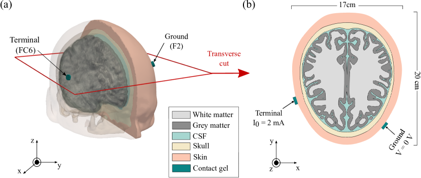
Figure 1: Geometrical models of the head. (a): 3D model head model (with sagittal cut). The axial cut plane shown was used to build the 2D model.(b): 2D brain model including the segmented brain tissues. The tACS montage (position of electrodes and intensity applied at each electrode), dimension of the model and tissues modeled are illustrated.

The two models were imported into COMSOL Multyphysics (COMSOL Inc., MA, USA), which was used for the field computation and error analysis. Two cylinders of 1-cm-diameters represented the contact gel for compact electrodes and were placed over the FC6 and F2 positions (figure 1a; placement according to the international EEG 10-20 system [38]). The electrodes were represented as semi-rectangular domains in the 2D model (figure 1b). Electrodes were modeled in terms of corresponding Dirichlet boundary conditions on exterior edge of the gel [39].

Finally, the surface mesh was generated using an L2 norm of error squared based mesh refinement in COMSOL Multiphysics, which lead to 125k triangular elements for the 2D model. The 3D model was meshed with 5.31M tetrahedron elements. The smallest element edge was 0.5 mm and the largest one was 5 mm. This ensures convergence while having maximum element size much smaller than one tenth of the wavelength in each tissue for the highest considered frequency of 100 MHz.

2.2 Electric field modeling

The electric field analysis requires a prior specification of the tissue dielectric properties [conductivity $\sigma$ (S/m) and relative permittivity $\varepsilon_{r}$]. Since this study requires taking into account the dispersion due to the wide frequency range of interest, we choose the established four-region Cole–Cole model with the coefficients tabulated by S. Gabriel and co-workers [40] since it i) accounts for dispersive effects of tissues, ii) allows to quantify the error introduced by neglecting the relative permittivity, iii) satisfies the required Kramers–Kronig relationship [41]. The conductivity of the contact gel was set to 1.4 S/m [42] and the relative permittivity to 80 as salt water. Note that another important factor that might influence the estimated errors are the assumptions about the tissue electric properties. The low-frequency values (i.e., DC to tenth of kHz) found in the literature vary considerably [43], sometimes almost one order of magnitude, due to different conditions of the tissue and different ways of measuring. In particular, this set of conductivities is reported to deviate from literature in the low frequency range. To analyze the effect of dielectric properties variation on the relative error, we performed the analysis at 10 Hz with some of the extreme cases reported in literature to indicate the range of electric field variation due to dielectric properties uncertainty.

The first formulation tested is the most used for tCS: the static formulation that neglects the propagating effect ($\lambda\ll a$) as well as the capacitive effect of tissues, i.e., the contribution of the relative permittivity ($\sigma\gg\omega\varepsilon_{r}$). The second is the quasi-static (QS) formulation, which only neglects the propagative effects, but not the permittivity contribution since the ratio between $\sigma$ and $\varepsilon_{r}$ (representing the dielectric relaxation time) is not negligible as compared to the typical variations of the electric field. This is also equivalent to considering a complex conductivity $\sigma_{c}=\sigma+j\omega\varepsilon_{r}$. The third and the most general formulation consists of solving the inhomogeneous wave equation for the electric field, which is equivalent to solving the full set of Maxwell equations or full wave formulation (FW).

For both static and QS formulations, the Laplace equation for the electric potential V [$\nabla\cdot(\sigma_{c}\nabla V)=0$] was solved providing boundary conditions as follows:

• A Dirichlet boundary condition to model the ground (or cathode, $V=0$);

• A modified Dirichlet boundary condition (terminal boundary condition) on the anode, which imposes a constant current source ($\int\textbf{J}\cdot d\textbf{S}=0$) with a calculated fixed potential;

• An insulation boundary condition (Neumann) $\textbf{J}\cdot d\textbf{S}=0$ on the remaining boundaries to model the skin–air interface.

A stabilized formulation at low frequency (below 1 MHz) was used in FW computations, which is similar to the one described in [44, 45] since common FW formulations are known to be unstable at low frequencies [46, 47]. The wave equation was decomposed into electric and magnetic vector potentials and solved on potentials rather than on the field directly. This formulation consists of solving Maxwell–Ampere’s equation along with its divergence on electric and magnetic vector potentials, and appropriate boundary conditions as previously described supported with a Dirichlet boundary condition on the magnetic vector potential ($\textbf{A}\times\textbf{n}=0$).

The three formulations were solved on a mesh containing over 289k triangular elements for the 2D model and 5.31M of tetrahedrons elements for the 3D model. MUMPS numerical solver was used to solve the linear system for the frequency range from 10 Hz to 100 MHz with 10 values per decade and with a relative tolerance of $10^{-6}$ for the 2D model. For the 3D model, appropriate iterative solvers formulation (Conjugate Gradient for static, BiCStab for QS and GMRES for FW) were used according to the formulation, with a relative tolerance of $10^{-6}$. Finally, the relative error of the imposed approximation was computed using $\eta_{12}=||\textbf{E}_{1}-\textbf{E}_{2}||/||\textbf{E}_{1}||$ where 1 denotes the reference, being either FW when compared to the other formulations, or QS to compute the relative error between static and QS. The resulting error was computed over the whole numerical domain for each frequency, and the following metrics were computed: minimum, maximum, $2.5^{\mathrm{th}}$ quantile, $97.5^{\mathrm{th}}$ quantile, and mean.

An additional study was performed to account for the electrode positioning. The skin contour curve, defined by the two coordinates (x, y), was interpolated according to the angle $\theta$ defined by the three following points: the fixed point in the frontal part of the head representing the cathode’s center, the center of the head and a third moving point on the contour. The latter represents the center of the anode which was moved to study the influence of the placement. See section 3.2 for the schematic of the setup.

2.3 Time domain waveform and harmonics

Despite the typical use of sinusoidal signals in the case of tACS, temporal waveforms analysis might be useful for the elaboration of new techniques relying on waveform shaping to optimize the current delivery or even for shorter pulses used in intersectional tDCS (IS-tDCS) [31]. Once the electric field was computed for each formulation, the electric field values were exported from Lagrange’s points (vertices) of the mesh [48]. A post-processing routine was developed to convert these frequency-domain data into the time domain using Fourier series as:

$$s(t)=\sum_{n}{c_{n}e^{2i\pi tf_{n}}+c_{-n}e^{-2i\pi tf_{n}}},$$

where $f_{n}$ is the frequency of the $n^{\mathrm{th}}$ harmonic and $c_{n}$ the associated Fourier’s coefficient. Fourier series were used to compute the electric field for typical time domain waveforms used for DBS, namely monophasic and biphasic pulses. Pulse parameters were chosen in accordance with typical DBS waveform parameters: pulse duration was 90 µs, and the frequency was set to 130 Hz, which was comparable to the values used in [29], with the same highest harmonic at 500 kHz and a sampling frequency of 1MHz. Then, the relative error was computed in the time domain in the same way than in the frequency domain, for each time step between 0 to 400 µs.

2.4 Impact on neuromodulation

Electric field modeling during tACS is commonly accompanied by radial electric field calculation from the EF distribution [11]. This radial EF (EF component normal to the cortex surface) represents the EF along the pyramidal cells, which have a strongly preferential orientation normal to the cortex and are organized. These cells showed the highest membrane polarisation due to the electric field with a direction parallel to their somato-dendritic orientation [10], which makes it a measure of tCS effect. The radial electric field error was assessed similar to the previous relative error metric as $\eta_{12}=||\textbf{E}_{r1}|-|\textbf{E}_{r2}||/|\textbf{E}_{r1}|$. The variation from the previous relative error formula was the difference of absolute values, i.e., the radial EF amplitude without taking into account the phase difference. The impact of tACS was located at the cortex level where the field is the highest. The 98^th EF quantile was computed over the cortical surface, and points with higher EF were selected to compute the radial relative error where accurate values are needed to predict the effect at the neuron level. We additionally assessed the same metric for the tangential component and the resulting angle between the electric field and the normal directions to the surface of the gray matter. Finally, the phase difference between the different formulations was quantified since the phase term could have impact on phase activity [49] and is supposed to not vary with location in the common static case.

To highlight the importance of these results, we performed neural modeling with a realistic neuronal model [50] using the established NEURON software [51]. Pyramidal cell from the 5^th cortical layer was used as it was demonstrated to be responsive to a 10 Hz tACS [52]. The same mechanisms and setup were used as in [52]: a synaptic input was chosen to generate a 5Hz activity and the extracellular mechanism was used to input the EF in the form of potential. A 10 Hz tACS was used and values of EF were set using radial relative error results. Three simulations were performed for three different EF amplitudes: 1.00 V/m as the reference, the additional average error on the radial field, and the maximum one. Each simulation consisted of 140 seconds: 10 seconds of off stimulation and 2 minutes of on tACS and 10 seconds of off tACS. Then, the phase-locking value (PLV) was computed to quantify the impact of tACS on neuron firing times, along with polar plots to quantify the timing influence of the stimulation.

3 Results

3.1 Relative error spectrum

Electric field maps were calculated over the considered frequency range, and the $97.5^{\mathrm{th}}$ and $2.5^{\mathrm{th}}$ quantiles in addition to the mean relative error are illustrated in figure 2. Both the relative error between FW and QS ($\eta_{\mathrm{FWQS}}$) and between static and QS ($\eta_{\mathrm{SQS}}$) are represented for the 2D and 3D models for the FC6–F2 montage. The relative error between FW and static, $\eta_{\mathrm{SFW}}$, is not shown because it is overlapping with $\eta_{\mathrm{SQS}}$ since $\eta_{\mathrm{FWQS}}\ll\eta_{\mathrm{SQS}}$. The results for 2D and 3D models are in very good agreement, which validates the use of the simplified 2D model for the subsequent studies requiring prohibitive computations over the 3D mesh. The average of $\eta_{\mathrm{SQS}}$ was over 20% in brain tissues within the frequency range of 10–40 Hz – a common range used for tACS since it corresponds with the frequencies of physiological brain oscillations (and so is $\eta_{\mathrm{SFW}}$).

In contrast, $\eta_{\mathrm{FWQS}}$ increases with frequency and crosses the 1% error line in the MHz range. Table 1 summarizes 1%, 5% and 10% limits for the multiple metrics described in the previous section. These metrics can be used to define the range of the QSA validity, depending on the error level that should not be exceeded.

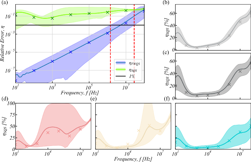
Figure 2: (a): Relative error spectrum between quasi-static and full wave approaches ($\eta_{\mathrm{FWQS}}$) and between static and quasi-static ($\eta_{\mathrm{SQS}}$), $f$ being the frequency. The mean error, the $97.5^{\mathrm{th}}$ and $2.5^{\mathrm{th}}$ quantiles for both $\eta_{\mathrm{FWQS}}$ and $\eta_{\mathrm{SQS}}$ with solid lines for the 2D model while the crosses represent the results for the 3D model. The 1% percent error line is shown and intersections between the $97.5^{\mathrm{th}}$ and $2.5^{\mathrm{th}}$ quantiles for $\eta_{\mathrm{FWQS}}$ is depicted as dotted red lines at 1.43 MHz and 28.16 MHz, respectively. (b) to (f): $\eta_{\mathrm{SQS}}$ in each tissue layer (in the order: WM, GM, skin, skull and CSF) for the 2D model (solid lines and quantiles) and 3D model (crosses).

Table 1: Frequencies (MHz) at which the minimum, maximum, mean, 2.5^th and 97.5^th quantiles FW to QS relative error cross 1%, 5%, and 10%, respectively

• $\eta_{\mathrm{FWQS}}$	Min	$q_{\mathrm{2.5}}$	Avg	$q_{\mathrm{97.5}}$	Max
  1%	$>100$	28.16	5.13	1.43	0.81
  5%	$>100$	86.63	17.04	5.92	3.74
  10%	$>100$	$>100$	27.97	10.04	6.71

3.2 Effect of dielectric properties variability

The high relative error between static and quasi-static formulations is mainly due to the low values of electric conductivities of brain tissues in the used set of dielectric values. To investigate the range of SQS relative error over the range of conductivities reported in the literature, we performed the simulation at 10 Hz with the extreme dielectric properties for GM, WM, skull, and skin. As the reported values of CSF do not vary significantly, we kept the conductivity and relative permittivity values at 1.654 [S/m] and 102, respectively, throughout this analysis). For GM, WM, skull, and skin, the range of conductivities was taken from [43]. On the other hand, the relative permittivities were set with reasonable extreme values due to the lack of litterature data on this parameter in the Hz range. All the considered values are presented in the table 2.

Table 2: Extreme dielectric properties used to asses the range of SQS relative error at 10 Hz.

• 	$\sigma$ GM	$\sigma$ WM	$\sigma$ Skull	$\sigma$ Skin	$\varepsilon_{r}$ GM	$\varepsilon_{r}$ WM	$\varepsilon_{r}$ Skull	$\varepsilon_{r}$ Skin
  min	0.06	0.0642	0.0182	0.137	$10^{5}$	$10^{5}$	$10^{3}$	$10^{2}$
  max	2.47	0.81	0.28	2.1	$10^{8}$	$10^{8}$	$10^{5}$	$10^{4}$

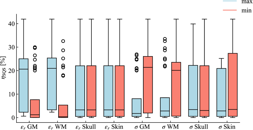
Figure 3: Mean SQS Relative error at 10 Hz for all the extreme conductivity and relative permittivity values combination. The blue boxes represent the distribution for all the case where the maximum value of the property was used while the red correspond to the cases where the minimum value was used.

The distributions of the mean error, depicted figure 3, show higher errors for higher relative permittivity and lower conductivity, which is in agreement with the change in effective conductivity $\sigma_{c}=\sigma+j\omega\varepsilon$. It can also be observed that bimodal distributions occur when using minimum relative permittivities and maximum conductivities for brain tissues. This is mainly due to the fact that the ratio between $\omega\varepsilon_{r}$ and $\sigma$ is at maximum, which occurs when the conductivity and permittivity values are both at their minima or maxima. These results show a possible relative error at 10 Hz bounded between $2.10^{-3}$% to 41.9% depending on the considered properties and further confirms the need of reliable measurement of tissue dielectric properties in the sub-kHz frequency range.

3.3 Influence of electrode positioning and size

Next, we investigated the influence of the electrode montage on the approximation error. The relative error variation was quasi symmetrical with respect to the $\theta=180^{\circ}$ axis. This motivated to choose a parameter varying as symmetrically such as the euclidean distance between the spatial positions of the two scalp electrodes, denoted as d (see figure 4a and 3c. Figure 3b depicts that the relative error between QS and FW decreases as the distance between the two electrodes increases.

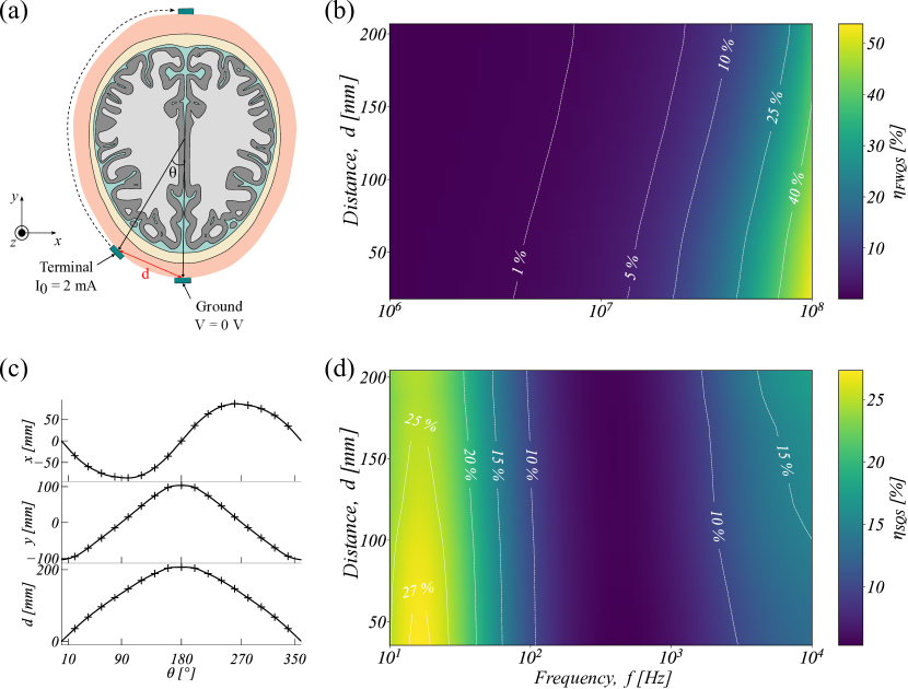
Figure 4: (a): 2D model with the angle defining the position of the anode by reference to the cathode position. (b): Relative error between FW and QS ($\eta_{\mathrm{FWQS}}$) as a function of the distance (d) between anode and cathode in the 1–100 MHz range. The distance between the two electrodes is taken as the vertical axis, while the frequency $f$ in log space in horizontal axis. (c): x and y coordinates of the skin curve depending on theta and the associated euclidean distance. (d): Relative error between static and QS ($\eta_{\mathrm{SQS}}$) in the 10-Hz–10-kHz range, as illustrated with the previous plot.

Conversely, $\eta_{\mathrm{SQS}}$ has non monotonic variations at low frequency (below 10 kHz). In the 10–100 Hz range, the error is higher with proximal electrodes but the effect is reversed in the kHz range as illustrated figure 4d. The increase of $\eta_{\mathrm{SQS}}$ at the skin level in the kHz can explain this since the current is more distributed in skin when the electrode are more spaced. Conversely, with proximal electrodes, the electric field is less distributed in skin and the error is more represented by the one in the GM at low frequency.

This study considers $\diameter 1$ cm electrodes. In order to evaluate if the error is affected by the electrode size, we performed an additional analysis with $\diameter 2$ cm as it is another standard size for circular electrodes. No sensible variation in error was found, which indicates a negligible effect of the electrode size on QSA validity.

3.4 Error for typical time-domain waveforms

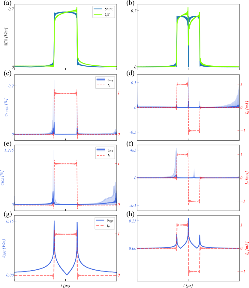
Figure 5: (a)–(b): $97.5^{\mathrm{th}}$ highest electric field norm ($||E||$) in grey matter for monophasic (a) and biphasic (b) pulses in Static and QS cases. (c)–(d): Average relative error between FW and QS ($\eta_{\mathrm{FWQS}}$) in the time domain for (c) a monophasic pulse as a stimulus, and (d) a biphasic pulse, with the $2.5^{\mathrm{th}}$ to $97.5^{\mathrm{th}}$ quantile margin. The stimulus is represented in red with its corresponding second axis. (e)–(f): As (c)–(d) for the case of relative error between Static and QS ($\eta_{\mathrm{SQS}}$). (g)–(h): Norm of the difference of the $97.5^{\mathrm{th}}$ quantile electric fields ($\delta_{\mathrm{SQS}}$) in the grey matter.

Using the Fourier’s series decomposition, the time domain relative error between QS and FW remained below 1% for both square and biphasic pulses; figure 5 demonstrates the general trends. The error was higher before and after the pulse with the highest values during the ascending and descending parts of the pulse, and smaller one during the positive phase of the pulse. This might originate from the difference in phase with the zero crossing of the finite harmonics signal. This is even more pronounced in the case of $\eta_{\mathrm{SQS}}$, which is tremendous due to zero crossings occurring at different times for Static and QS. Since it is mainly due to error in phase, it does not reflect properly the amplitude error, which is only represented during the positive phase of the pulse (and down state for the biphasic pulse), where the signal does not cross zero. This further justifies the choice made by Bossetti et al. [29] to represent the relative error only during positive state of the pulse. However, it does not highlight the error during at pulse termination which is substantial. Figure 5 shows that the results are in good agreement with [29], at least at the brain level where $\eta_{\mathrm{SQS}}$ decrease from 14% during the first part of the pulse positive phase while increasing during the second part and flare-up at the pulse termination. This is mainly due to the zeros crossing of the pulse due to Gibb’s phenomenon. The norm of the difference between the compared electric field does not suffer from the aforementioned limitations and quantify an error in electric field unit. It is directly related to the amount of EF which is not present at the neuron level, and proportional to the membrane depolarisation. Figure. 4g and 4f illustrate this difference in electric field norm in the case of the $97.5^{\mathrm{th}}$ highest electric field, which is the zone where stimulation has the greatest impact. This difference is of the same order of magnitude than the electric field itself, which is significant and represents a difference of 22.7% with the maximum value of the positive phase for a monophasic pulse (Static case) and 42.9% for the biphasic pulse.

Figure 6: SQS relative error ($\eta_{\mathrm{SQS}}$) during the monophasic pulse up-state in the GM. The horizontal axis is the time $t$ relative to the beginning of the pulse (0 being the start of the pulse). The mean value is plotted as a solid line and the margin represent the $97.5^{\mathrm{th}}$ and $2.5^{\mathrm{th}}$ quantiles.

3.5 Radial relative error

The radial, tangential and angle relative errors computed on the highest 2% EF values over the cortical surface shows similar trends as over the full gray matter domain; The results are presented in figure 7 where the min–max margins over the 2D models and crosses for the 3D model are shown for all the six resulting errors. The curve for the average relative errors over the full cortex (all the EF values) are plotted as the green dashed line and is encompassed by the margins for $\eta_{\mathrm{SQS}}$ while it is slightly above the maximum in the case of the FWQS radial relative error. At 10 Hz, which is a common frequency used for tACS [52], the average radial relative error for the 2% highest EF was about 6% while the maximum reached 22% in the case of SQS. The tangential relative error is higher with an even larger maximum in the full spectrum [figure 7(c) and (d)]. The average error (solid line) share same trend. Note that this higher maximum error can be due to the small absolute values of tangential field compared to the radial one, and relative error metrics are more sensitive to small field values. As a consequence, this impacts the error on the field orientation (angle between radial and tangential fields), which share the same trend. For the FW to QS, the average radial relative error remained below 1% until 10 MHz, while the tangential and angle relative errors cross the line at 7.24 and 5.01 MHz, respectively.

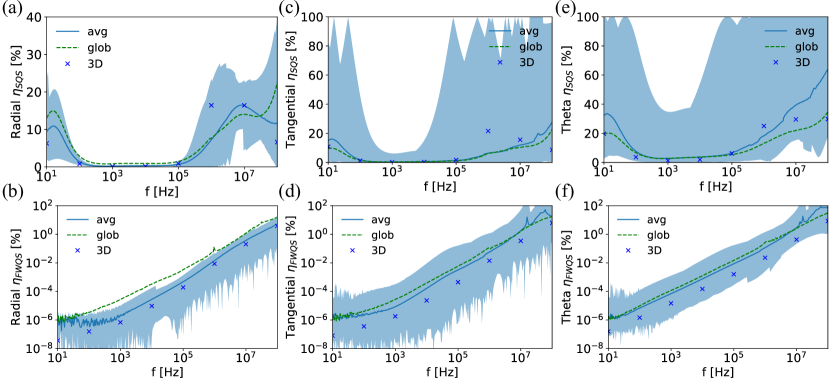
Figure 7: Radial relative error between static and QS predictions (a) and between QS and FW (b). The continuous and dashed lines correspond to the 2D model results while the crosses represent the average radial relative error in the 3D model. The dashed green lines represent the average radial relative error over the full cortex. The same applies to tangential relative error for SQS (c) and FWQS (d) as well as for the angle SQS (e) and FWQS (f) relative errors

Finally, the phase error is depicted figure 8 and shows the same trends as previous cases. To quantify the phase error, we use absolute absolute difference in radians between 1) QS and static [SQS in figure 8(a)] and 2) FW and QS [FWQS, figure 8(b)].

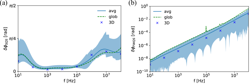
Figure 8: Phase difference (in radians) between static and QS, $\delta\phi_{\mathrm{SQS}}$ (a) and FW and QS, $\delta\phi_{\mathrm{FWQS}}$ (b).

The average of SQS phase difference is up to $\pi/8$ in the 10–100 Hz frequency range. Its maximum is up to $\pi/4$, which represents a non-negligible phase difference from the neuromodulation point of view. Specifically, the neuron populations are stimulated with different phases depending on their location, which static approximation neglects. However, in the FWQS case, the phase difference is quite negligible and increase log-linearly to cross a 1% difference at 13.18 MHz.

3.6 Effect of tACS on single neuron activity

Using the previous results as an input for neural activity modeling of the selected pyramidal cell, the neural activity during tACS was computed with 1.00, 1.06 and 1.22 V/m. All spike timing event were saved and then used to compute the distribution of spikes occurring in the same range of tACS waveform phase. The corresponding polar plots are depicted in figure 9 with the neuron morphology. The distributions are close to each other since the sub-threshold input due to the extracellular field has little effect [12]. However, the calculated PLV for each amplitudes are 0.0640, 0.0716, and 0.0798, respectively, which correspond to a 10.48% increase in PLV for the average radial relative error and 19.66% increase for the maximum one. These results show the need of reliable EF predictions and the impact of taking into account the relative permittivity.

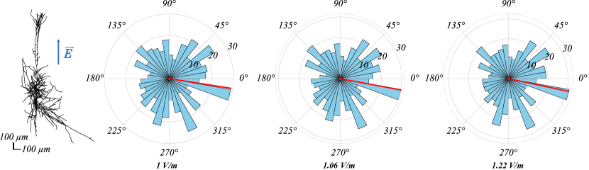
Figure 9: Polar plots of the phase of spike occurrences distributions for the three different EF amplitude. The morphology is depicted in the left part with the direction of the input EF. Polar histograms correspond to event counts while the red line is the phase of the average vector.

4 Discussion

The major goal of this study was to assess the frequency-dependent accuracy of static and QS approximations commonly used in the tCS numerical analysis. We evaluated the tCS-induced electric fields in heterogeneous anatomical models for static, QS, and FW approximations. In terms of the error limits, the QSA 1% error limit stands up to the MHz range exceeding 1% at 5.16 MHz for the mean and at 1.43 MHz for the $97.5^{\mathrm{th}}$ quantile. This agrees well with the literature, where the limit at 1% was identified using a plane wave illumination at 10 MHz [53]. In terms of the error between two possible QSA formulations – depending on whether one neglects the capacitive effect of tissues – we demonstrated, for the first time, that $\eta_{\mathrm{SQS}}$ is significant and even exceeds $\eta_{\mathrm{FWQS}}$ in the case of tCS. This is an important takeaway, since the inclusion of capacitive effects in the model does not significantly increase computational costs, especially as compared to a computationally expensive FW approach.

The FWQS relative error shows a linear-log increase over the frequency spectrum, as expected, since it is often quantified as being proportional to $\omega^{2}$ [54], confirming the validity of QSA below the MHz range without neglecting capacitive effects. The interpretability of the SQS relative error is less straightforward, since it is mainly due to the change in the current distribution that is affected by the intrinsic impedance change. Note that in the low frequency range, in which tACS is currently performed (10–100 Hz), the SQS relative error is about 20% for the 3D model, and it increases up to 50% for the $97.5^{\mathrm{th}}$ quantile of the 2D model (figure. 2c) in the brain. In high EF intensity areas, i.e. where brain is stimulated, this error can be as high as 22% in the radial direction which therefore affects the firing times of pyramidal cells as demonstrated here. We hope that these results should encourage to consider the capacitive effect of tissues even at very low frequencies, since the relative permittivity is sufficiently high to induce significant errors in both amplitude and phase of induced electric field. Since EEG and tES are related by the reciprocity principle [55, 56], EEG source localization methods could also be impacted by this error. Currently, these methods are often formulated using purely ohmic tissues [57, 58]. However, this frequency dependence would drastically increase the computational cost in this inverse problem. It remains an open question how considering this frequency dependence of the permittivity would improve the performance of EEG source localization methods. The static approach might be still preferred for highly repetitive 3D modeling, such as the optimization of electrode placement [59]. In this case, an additional post-optimization QSA analysis might still be useful to provide more accurate values of electric field distribution.

The FWQS error was found to be a function of the distance between two electrodes, however limits remained within the same range (1–10 MHz for 1% error, for example). The distance-error dependence also affected $\eta_{\mathrm{SQS}}$ at low frequencies. In the EEG spectrum domain (10–50Hz), the error decreased with distance, which can be explained by the higher error in the brain being more represented in the average one. This even increased the error in the case of high definition tCS, where one electrode is closely surrounded by four others to increase focality of conventional tCS [18, 60]. This is a technique that is mainly used at low frequency (within the EEG frequency range: typically from DC to 100 Hz). Conversely, $\eta_{\mathrm{SQS}}$ increased as the electrodes were moved away in the frequency range used for the temporal interference technique (1–10 kHz). This is mainly due to the increase of $\eta_{\mathrm{SQS}}$ in this frequency range in skin where the electric field is more distributed due to the electrode spacing.

Finally, the computed electric field in the Fourier space (frequency domain) can be transformed into the time domain and used to compute the corresponding relative errors. Here, we presented two examples with 1) the monophasic pulse studied in [29] for comparison and 2) the biphasic pulse that is a typical waveform used in brain stimulation and, in particular, for DBS [61]. The results in the time domain suggest that the resulting error from using QS over FW was less than 1%, validating the use of the QSA for this purpose. This level of numerical error is lower than 13% reported by [29] during the positive phase of the pulse. However, this difference is due to the comparison between the Static and FW formulations. In our case, the error quantification showed a comparable range of error in grey matter supporting the rationale to include capacitive effects when the relative permittivity at low frequencies is high. This supports the previous statements that neglecting the capacitive effect of tissues can be considered as an unreasonable approximation for most cases [21, 29].

This study addressed the question of the approximation for tCS electric field modeling in the case of a realistic head model with the main five tissues used in the literature. The use of the Cole–Cole model can be criticized, since deviations in conductivity have been identified at low frequencies ($<1$ MHz) [40], which could be attributed to electrode-electrolyte interface during measurements [23, 62]. This issue was recently addressed by compensating this electrode–electrolyte interface impedance [62], which opens the possibility to use corrected values. However, another study reported similar range of values for relative permittivity but higher conductivities than the initial measurements, in mice tissues [24] and is physically plausible. Purely ohmic tissue models are plausible but singular due to Kramers–Kronig relations [41]. Still, in this model, skin has a conductivity of the order of $10^{-4}$ S/m, whereas it is commonly set in the 0.2–0.5 S/m range [18, 63, 64]. This could be explained by the fact that scalp tissues are multilayered, and composed of multiple tissues with their own properties, and that only surface skin was measured. Yet, the conductivity used in Static and QS model are the same and we assess the QSA validity using a relative metric which is expected to be as high, even if more current is shunted through the scalp. This illustrates further the need for reliable values of conductivity/permittivity at low frequency, where there is a large dispersion of values. It is also worth to point out that most values were measured post-mortem, which can affect the results [24]. Another source of variability is inter-individual differences in brain morphology and conductivity [65], especially since such variability could be a larger source of error than these tackled approximations [66] and impact substantially the electric field distribution [67]. To overcome this limitations, we used a standardized (template) brain model, since the aim of this study was to show the intrinsic limitations of modeling practices, and the general tendencies of the error induced by the use of approximations, and not to extend exact values for every singular geometric model. Finally, multiple electrodes stimulation montages could also be studied as an extension of the present study, since electrode positioning has been shown to have an important impact on the relative error distribution, especially comparing Static to QS.

5 Conclusion

This study provided an insight into modeling approximations commonly made in the research field of tCS. We demonstrated the validity of quasi-static approximation of Maxwell’s equations until the MHz range if the relative permittivity is considered. However, the static approximation (i.e., purely resistive medium, no capacitive effects), introduces significant errors in tACS modeling in both the electric field amplitude and the phase. More importantly, static approximation assumes that the phase of induced electric field is the same across the brain. Our results demonstrate that the phase can vary up to $\pi/4$ across the different regions of the brain, which is significant from the point of view of neuromodulation. Considering capacitive properties (i.e., relative permittivity of tissues, or, equivalently, the imaginary part of the conductivity) is especially important for pulsed signals that contain multiple frequency harmonics. Finally, precise knowledge of approximation-induced errors contributes to the better accuracy of computational modeling in tCS and therefore the analysis of associated effects at the cellular level.

Appendix: Maxwell’s equations theory and approximations

This appendix summarizes the equations for the electric field depending on the assumptions made in the article. We start from the general set of Maxwell’s equations to derive the ones used in approximations stated here as ”static” and ”quasi-static.” The four Maxwell’s equation can be written as:

$$\nabla\cdot\mathbf{D}=\rho \qquad(\mathrm{Maxwell\!-\!Gauss})$$ (1)

$$\nabla\times\mathbf{E}=-\frac{\partial\mathbf{B}}{\partial t} \qquad(\mathrm{Maxwell\!-\!Faraday})$$ (2)

$$\nabla\cdot\mathbf{B}=0 \qquad(\mathrm{Maxwell\!-\!Thomson})$$ (3)

$$\nabla\times\mathbf{H}=\mathbf{J}+\frac{\partial\mathbf{D}}{\partial t} \qquad(\mathrm{Maxwell\!-\!Ampere})$$ (4)

where $\mathbf{D}$ is the electric displacement field, $\mathbf{E}$ the associated electric field, $\mathbf{H}$ being the magnetic field, which is related to the magnetic flux density $\mathbf{B}$. The conservation of the charge is obtained by taking the divergence of (4):

$$\nabla\cdot\nabla\times\mathbf{H}=0=\nabla\cdot\mathbf{J}+\frac{\partial\rho}{\partial t}$$ (5)

Generally, the Maxwell’s equations in time domain are computationally expensive to solve since the solution involves time convolution with electrical properties [68]. In practice, the Fourier transform of the equations is computed since it involves a simple multiplications in the generalized Ohm’s law $\mathbf{J}=\sigma\mathbf{E}$ and constitutive equations $\mathbf{D}=\varepsilon\mathbf{E}$ and $\mathbf{B}=\mu\mathbf{H}$ for linear media. This also simplifies the partial time derivatives, which are now simple multiplications with $j\omega$. In this study, we consider biological tissues that have a constant magnetic permeability $\mu=\mu_{0}$ but do not have constant relative permittivity. Considering that both $\sigma$ and $\varepsilon$ are functions of the frequency, the medium for which the equations are solved is dispersive. This is the most general case without any other assumption other than media linearity. Therefore, considering (1) and (4), (5) can be written as:

$$\nabla\times\mathbf{H}=\sigma\mathbf{E}+j\omega\varepsilon\mathbf{E}$$ (6)

$$\nabla\cdot\left[\left(\sigma+j\omega\varepsilon\right)\mathbf{E}\right]=0$$ (7)

The electro-quasistatic (EQS) approximation from the electromagnetics point of view consists in neglecting the effect of the induction on the electric field [27, 28]. This is reflected by the following change in (3):

$$\nabla\times\mathbf{E}=0$$ (8)

It implies that E is a gradient of a scalar field, i.e., the usual relation to the scalar potential in quasi-static: $\mathbf{E}=-\nabla V$. At this point, considering a dielectric medium, this results in the Laplace equation on the scalar potential by using (7):

$$\nabla\cdot[(\sigma+j\omega\varepsilon)\nabla V]=0$$ (9)

This simplification involves a spatial differential equation on a scalar quantity and is the equation solved for ”quasi-static” case as referred to in the present work. In the neuromodulation research community, any form of Laplace equation is often cited as being the consequence of quasi-static assumptions. Additional assumptions are also considered to have an even simpler equation. Indeed, often no dispersion is used (no frequency dependence of $\sigma$ and $\varepsilon$) together with neglecting the relative permittivity, i.e. assuming $j\omega\varepsilon/\sigma\ll 1$. This results in the Laplace equation on potential typically used in tACS numerical modeling:

$$\nabla\cdot(\sigma\nabla V)=0$$ (10)

Eq. (10) formalizes what is commonly meant as ”quasi-static assumption” in the neuromodulation community. Note that this contrasts with how EQS is defined in the electromagnetics/physics community, which often relates to this equation as ”static regime” or ”quasi-stationary conduction” [27]. Since in this study we analyze the accuracy of both (9) and (10), we use the terms ”static” and ”quasi-static,” respectively, in the text to distinguish these two approaches.

References

References

- [1] Marom Bikson, Pnina Grossman, Chris Thomas, Adantchede Louis Zannou, Jimmy Jiang, Tatheer Adnan, Antonios P. Mourdoukoutas, Greg Kronberg, Dennis Truong, Paulo Boggio, André R. Brunoni, Leigh Charvet, Felipe Fregni, Brita Fritsch, Bernadette Gillick, Roy H. Hamilton, Benjamin M. Hampstead, Ryan Jankord, Adam Kirton, Helena Knotkova, David Liebetanz, Anli Liu, Colleen Loo, Michael A. Nitsche, Janine Reis, Jessica D. Richardson, Alexander Rotenberg, Peter E. Turkeltaub, and Adam J. Woods. Safety of transcranial Direct current stimulation: evidence based update 2016. Brain Stimulation, 9(5):641–661, September 2016. Number: 5.
- [2] Djamila Bennabi and Emmanuel Haffen. Transcranial direct current stimulation (tDCS): A promising treatment for major depressive disorder? Brain Sciences, 8(5), May 2018.
- [3] Paulo S. Boggio, Alice Nunes, Sergio P. Rigonatti, Michael A. Nitsche, Alvaro Pascual-Leone, and Felipe Fregni. Repeated sessions of noninvasive brain DC stimulation is associated with motor function improvement in stroke patients. Restorative Neurology and Neuroscience, 25(2):123–129, 2007.
- [4] Hyo Keun Lee, Se Ji Ahn, Yang Mi Shin, Nyeonju Kang, and James H. Cauraugh. Does transcranial direct current stimulation improve functional locomotion in people with Parkinson’s disease? A systematic review and meta-analysis. Journal of Neuroengineering and Rehabilitation, 16(1):84, July 2019.
- [5] Nicole R. Nissim, Andrew O’Shea, Aprinda Indahlastari, Jessica N. Kraft, Olivia von Mering, Serkan Aksu, Eric Porges, Ronald Cohen, and Adam J. Woods. Effects of transcranial direct current stimulation paired with cognitive training on functional connectivity of the working memory network in older adults. Frontiers in Aging Neuroscience, 11:340, 2019.
- [6] M. A. Nitsche and W. Paulus. Excitability changes induced in the human motor cortex by weak transcranial direct current stimulation. The Journal of Physiology, 527(3):633–639, September 2000. Number: 3.
- [7] M. A. Nitsche. Catecholaminergic consolidation of motor cortical neuroplasticity in humans. Cerebral Cortex, 14(11):1240–1245, May 2004. Number: 11.
- [8] M. A. Nitsche, K. Fricke, U. Henschke, A. Schlitterlau, D. Liebetanz, N. Lang, S. Henning, F. Tergau, and W. Paulus. Pharmacological modulation of cortical excitability shifts induced by transcranial direct current stimulation in humans. The Journal of Physiology, 553(Pt 1):293–301, November 2003. Number: Pt 1.
- [9] Michael A. Nitsche, David Liebetanz, Anett Schlitterlau, Undine Henschke, Kristina Fricke, Kai Frommann, Nicolas Lang, Stefan Henning, Walter Paulus, and Frithjof Tergau. GABAergic modulation of DC stimulation-induced motor cortex excitability shifts in humans. European Journal of Neuroscience, 19(10):2720–2726, May 2004. Number: 10.
- [10] Marom Bikson, Masashi Inoue, Hiroki Akiyama, Jackie K. Deans, John E. Fox, Hiroyoshi Miyakawa, and John G. R. Jefferys. Effects of uniform extracellular DC electric fields on excitability in rat hippocampal slices in vitro: Modulation of neuronal function by electric fields. The Journal of Physiology, 557(1):175–190, May 2004. Number: 1.
- [11] Asif Rahman, Davide Reato, Mattia Arlotti, Fernando Gasca, Abhishek Datta, Lucas C. Parra, and Marom Bikson. Cellular effects of acute direct current stimulation: somatic and synaptic terminal effects. The Journal of Physiology, 591(10):2563–2578, May 2013. Number: 10.
- [12] Julien Modolo, Yves Denoyer, Fabrice Wendling, and Pascal Benquet. Physiological effects of low-magnitude electric fields on brain activity: Advances from in vitro, in vivo and in silico models. Current Opinion in Biomedical Engineering, 8:38–44, December 2018.
- [13] Jared Cooney Horvath, Jason D. Forte, and Olivia Carter. Evidence that transcranial direct current stimulation (tDCS) generates little-to-no reliable neurophysiologic effect beyond MEP amplitude modulation in healthy human subjects: A systematic review. Neuropsychologia, 66:213–236, January 2015.
- [14] T. Radman, Y. Su, J. H. An, L. C. Parra, and M. Bikson. Spike timing amplifies the effect of electric fields on neurons: Implications for endogenous field effects. Journal of Neuroscience, 27(11):3030–3036, March 2007. Number: 11.
- [15] Pedro Cavaleiro Miranda, Mikhail Lomarev, and Mark Hallett. Modeling the current distribution during transcranial direct current stimulation. Clinical Neurophysiology, 117(7):1623–1629, July 2006.
- [16] Abhishek Datta, Maged Elwassif, Fortunato Battaglia, and Marom Bikson. Transcranial current stimulation focality using disc and ring electrode configurations: FEM analysis. Journal of Neural Engineering, 5(2):163–174, June 2008.
- [17] Tim Wagner, Felipe Fregni, Shirley Fecteau, Alan Grodzinsky, Markus Zahn, and Alvaro Pascual-Leone. Transcranial direct current stimulation: A computer-based human model study. NeuroImage, 35(3):1113–1124, April 2007.
- [18] Abhishek Datta, Varun Bansal, Julian Diaz, Jinal Patel, Davide Reato, and Marom Bikson. Gyri-precise head model of transcranial direct current stimulation: Improved spatial focality using a ring electrode versus conventional rectangular pad. Brain Stimulation, 2(4):201–207.e1, October 2009.
- [19] Yu Huang, Lucas C. Parra, and Stefan Haufe. The New York Head—A precise standardized volume conductor model for EEG source localization and tES targeting. NeuroImage, 140:150–162, October 2016.
- [20] Alexander Opitz, Mirko Windhoff, Robin M. Heidemann, Robert Turner, and Axel Thielscher. How the brain tissue shapes the electric field induced by transcranial magnetic stimulation. NeuroImage, 58(3):849–859, October 2011. Number: 3.
- [21] Giulio Ruffini, Fabrice Wendling, Isabelle Merlet, Behnam Molaee-Ardekani, Abeye Mekonnen, Ricardo Salvador, Aureli Soria-Frisch, Carles Grau, Stephen Dunne, and Pedro C. Miranda. Transcranial current brain stimulation (tCS): models and technologies. IEEE Transactions on Neural Systems and Rehabilitation Engineering, 21(3):333–345, May 2013. Number: 3.
- [22] Leila Chaieb, Andrea Antal, Alberto Pisoni, Catarina Saiote, Alexander Opitz, Géza Gergely Ambrus, Niels Focke, and Walter Paulus. Safety of 5 kHz tACS. Brain Stimulation, 7(1):92–96, January 2014.
- [23] S Gabriel, R W Lau, and C Gabriel. The dielectric properties of biological tissues: II. Measurements in the frequency range 10 Hz to 20 GHz. Physics in Medicine and Biology, 41(11):2251–2269, November 1996.
- [24] Tim Wagner, Uri Eden, Jarrett Rushmore, Christopher J. Russo, Laura Dipietro, Felipe Fregni, Stephen Simon, Stephen Rotman, Naomi B. Pitskel, Ciro Ramos-Estebanez, Alvaro Pascual-Leone, Alan J. Grodzinsky, Markus Zahn, and Antoni Valero-Cabré. Impact of brain tissue filtering on neurostimulation fields: A modeling study. NeuroImage, 85:1048–1057, January 2014.
- [25] Robert Plonsey and Dennis B. Heppner. Considerations of quasi-stationarity in electrophysiological systems. The Bulletin of Mathematical Biophysics, 29(4):657–664, December 1967.
- [26] K. R. Foster and H. P. Schwan. Dielectric properties of tissues and biological materials: a critical review. Critical Reviews in Biomedical Engineering, 17(1):25–104, 1989.
- [27] Francesca Rapetti and Germain Rousseaux. On quasi-static models hidden in Maxwell’s equations. Applied Numerical Mathematics, 79:92–106, May 2014.
- [28] Scott E. Kruger. The Three Quasistatic Limits of the Maxwell Equations. arXiv:1909.11264 [physics], October 2019. arXiv: 1909.11264.
- [29] Chad A Bossetti, Merrill J Birdno, and Warren M Grill. Analysis of the quasi-static approximation for calculating potentials generated by neural stimulation. Journal of Neural Engineering, 5(1):44–53, March 2008.
- [30] Christopher R. Butson and Cameron C. McIntyre. Tissue and electrode capacitance reduce neural activation volumes during deep brain stimulation. Clinical Neurophysiology, 116(10):2490–2500, October 2005.
- [31] Mihály Vöröslakos, Yuichi Takeuchi, Kitti Brinyiczki, Tamás Zombori, Azahara Oliva, Antonio Fernández-Ruiz, Gábor Kozák, Zsigmond Tamás Kincses, Béla Iványi, György Buzsáki, and Antal Berényi. Direct effects of transcranial electric stimulation on brain circuits in rats and humans. Nature Communications, 9(1):483, December 2018.
- [32] Nir Grossman, David Bono, Nina Dedic, Suhasa B. Kodandaramaiah, Andrii Rudenko, Ho-Jun Suk, Antonino M. Cassara, Esra Neufeld, Niels Kuster, Li-Huei Tsai, Alvaro Pascual-Leone, and Edward S. Boyden. Noninvasive deep brain stimulation via temporally interfering electric fields. Cell, 169(6):1029–1041.e16, June 2017.
- [33] Gabriel Gaugain, Julien Modolo, and Denys Nikolayev. Temporal interference modeling error using purely conductive medium appoximation. In 2022 44th Annual International Conference of the IEEE Engineering in Medicine and Biology Society (EMBC), Glasgow, July 2022. IEEE.
- [34] Gabriel Gaugain, Julien Modolo, Maxim Zhadobov, Ronan Sauleau, and Denys Nikolayev. Effect of permittivity on temporal interference modeling. In Proc. BioEM 2022, Nagoya, June 2022.
- [35] Gabriel Gaugain, Lorette Quéguiner, Maxim Zhadobov, Ronan Sauleau, Julien Modolo, and Denys Nikolayev. Modeling accuracy of transcranial current stimumation: Static and quasi-static approximations errors. In Proc. BioEM 2021, Ghent, October 2021.
- [36] Vladimir Fonov, Alan C. Evans, Kelly Botteron, C. Robert Almli, Robert C. McKinstry, D. Louis Collins, and Brain Development Cooperative Group. Unbiased average age-appropriate atlases for pediatric studies. NeuroImage, 54(1):313–327, January 2011.
- [37] Axel Thielscher, Andre Antunes, and Guilherme B. Saturnino. Field modeling for transcranial magnetic stimulation: A useful tool to understand the physiological effects of TMS? In 2015 37th Annual International Conference of the IEEE Engineering in Medicine and Biology Society (EMBC), pages 222–225, Milan, August 2015. IEEE.
- [38] G. H. Klem, H. O. Lüders, H. H. Jasper, and C. Elger. The ten-twenty electrode system of the International Federation. The International Federation of Clinical Neurophysiology. Electroencephalography and Clinical Neurophysiology. Supplement, 52:3–6, 1999.
- [39] Guilherme B. Saturnino, André Antunes, and Axel Thielscher. On the importance of electrode parameters for shaping electric field patterns generated by tDCS. NeuroImage, 120:25–35, October 2015.
- [40] S Gabriel, R W Lau, and C Gabriel. The dielectric properties of biological tissues: III. Parametric models for the dielectric spectrum of tissues. Physics in Medicine and Biology, 41(11):2271–2293, November 1996.
- [41] Claude Bédard and Alain Destexhe. Generalized theory for current-source-density analysis in brain tissue. Physical Review E, 84(4):041909, October 2011.
- [42] Abhishek Datta, Julie M. Baker, Marom Bikson, and Julius Fridriksson. Individualized model predicts brain current flow during transcranial direct-current stimulation treatment in responsive stroke patient. Brain Stimulation, 4(3):169–174, July 2011.
- [43] Hannah McCann, Giampaolo Pisano, and Leandro Beltrachini. Variation in Reported Human Head Tissue Electrical Conductivity Values. Brain Topography, 32(5):825–858, September 2019.
- [44] Yanpu Zhao and W. N. Fu. A new stable Full-Wave Maxwell solver for all frequencies. IEEE Transactions on Magnetics, 53(6):1–4, June 2017.
- [45] Yanpu Zhao and Zuqi Tang. A novel gauged potential formulation for 3-D electromagnetic field analysis including both inductive and capacitive effects. IEEE Transactions on Magnetics, 55(6):1–5, June 2019.
- [46] Romanus Dyczij-Edlinger, Guanghua Peng, and Jin-Fa Lee. Efficient finite element solvers for the Maxwell equations in the frequency domain. Computer Methods in Applied Mechanics and Engineering, 169(3-4):297–309, February 1999.
- [47] Jianfang Zhu and Dan Jiao. Fast full-wave solution that eliminates the low-frequency breakdown problem in a reduced system of order one. IEEE Transactions on Components, Packaging and Manufacturing Technology, 2(11):1871–1881, November 2012.
- [48] Pavel Solin, Karel Segeth, and Ivo Dolezel. Higher-Order Finite Element Methods. Chapman and Hall/CRC, 0 edition, July 2003.
- [49] Luke Johnson, Ivan Alekseichuk, Jordan Krieg, Alex Doyle, Ying Yu, Jerrold Vitek, Matthew Johnson, and Alexander Opitz. Dose-dependent effects of transcranial alternating current stimulation on spike timing in awake nonhuman primates. Science Advances, 6(36):eaaz2747, September 2020.
- [50] Henry Markram, Eilif Muller, Srikanth Ramaswamy, Michael W. Reimann, Marwan Abdellah, Carlos Aguado Sanchez, Anastasia Ailamaki, Lidia Alonso-Nanclares, Nicolas Antille, Selim Arsever, Guy Antoine Atenekeng Kahou, Thomas K. Berger, Ahmet Bilgili, Nenad Buncic, Athanassia Chalimourda, Giuseppe Chindemi, Jean-Denis Courcol, Fabien Delalondre, Vincent Delattre, Shaul Druckmann, Raphael Dumusc, James Dynes, Stefan Eilemann, Eyal Gal, Michael Emiel Gevaert, Jean-Pierre Ghobril, Albert Gidon, Joe W. Graham, Anirudh Gupta, Valentin Haenel, Etay Hay, Thomas Heinis, Juan B. Hernando, Michael Hines, Lida Kanari, Daniel Keller, John Kenyon, Georges Khazen, Yihwa Kim, James G. King, Zoltan Kisvarday, Pramod Kumbhar, Sébastien Lasserre, Jean-Vincent Le Bé, Bruno R.C. Magalhães, Angel Merchán-Pérez, Julie Meystre, Benjamin Roy Morrice, Jeffrey Muller, Alberto Muñoz-Céspedes, Shruti Muralidhar, Keerthan Muthurasa, Daniel Nachbaur, Taylor H. Newton, Max Nolte, Aleksandr Ovcharenko, Juan Palacios, Luis Pastor, Rodrigo Perin, Rajnish Ranjan, Imad Riachi, José-Rodrigo Rodríguez, Juan Luis Riquelme, Christian Rössert, Konstantinos Sfyrakis, Ying Shi, Julian C. Shillcock, Gilad Silberberg, Ricardo Silva, Farhan Tauheed, Martin Telefont, Maria Toledo-Rodriguez, Thomas Tränkler, Werner Van Geit, Jafet Villafranca Díaz, Richard Walker, Yun Wang, Stefano M. Zaninetta, Javier DeFelipe, Sean L. Hill, Idan Segev, and Felix Schürmann. Reconstruction and Simulation of Neocortical Microcircuitry. Cell, 163(2):456–492, October 2015.
- [51] M. L. Hines and N. T. Carnevale. The NEURON simulation environment. Neural Computation, 9(6):1179–1209, August 1997.
- [52] Harry Tran, Sina Shirinpour, and Alexander Opitz. Effects of transcranial alternating current stimulation on spiking activity in computational models of single neocortical neurons. NeuroImage, 250:118953, April 2022.
- [53] Sang Wook Park, Kanako Wake, and Soichi Watanabe. Calculation errors of the electric field induced in a human body under quasi-static approximation conditions. IEEE Transactions on Microwave Theory and Techniques, 61(5):2153–2160, May 2013.
- [54] Richard P. Feynman. The Feynman lectures on physics. Volume 2: Mainly electromagnetism and matter. Basic Books, New York, the new millennium edition, paperback first published edition, 2011.
- [55] Andrea Cancelli, Carlo Cottone, Franca Tecchio, Dennis Q Truong, Jacek Dmochowski, and Marom Bikson. A simple method for EEG guided transcranial electrical stimulation without models. Journal of Neural Engineering, 13(3):036022, June 2016.
- [56] Jacek P. Dmochowski, Laurent Koessler, Anthony M. Norcia, Marom Bikson, and Lucas C. Parra. Optimal use of EEG recordings to target active brain areas with transcranial electrical stimulation. NeuroImage, 157:69–80, August 2017.
- [57] David Weinstein, Leonid Zhukov, and Chris Johnson. Lead-field Bases for Electroencephalography Source Imaging. Annals of Biomedical Engineering, 28(9):1059–1065, September 2000.
- [58] Christoph M. Michel and Denis Brunet. EEG Source Imaging: A Practical Review of the Analysis Steps. Frontiers in Neurology, 10:325, April 2019.
- [59] Guilherme Bicalho Saturnino, Hartwig Roman Siebner, Axel Thielscher, and Kristoffer Hougaard Madsen. Accessibility of cortical regions to focal TES: Dependence on spatial position, safety, and practical constraints. NeuroImage, 203:116183, December 2019.
- [60] Dylan Edwards, Mar Cortes, Abhishek Datta, Preet Minhas, Eric M. Wassermann, and Marom Bikson. Physiological and modeling evidence for focal transcranial electrical brain stimulation in humans: a basis for high-definition tDCS. NeuroImage, 74:266–275, July 2013.
- [61] Sol De Jesus, Michael S. Okun, Kelly D. Foote, Daniel Martinez-Ramirez, Jaimie A. Roper, Chris J. Hass, Leili Shahgholi, Umer Akbar, Aparna Wagle Shukla, Robert S. Raike, and Leonardo Almeida. Square Biphasic Pulse Deep Brain Stimulation for Parkinson’s Disease: The BiP-PD Study. Frontiers in Human Neuroscience, 13:368, October 2019.
- [62] Julius Zimmermann and Ursula van Rienen. Ambiguity in the interpretation of the low-frequency dielectric properties of biological tissues. Bioelectrochemistry, 140:107773, August 2021.
- [63] T.A. Wagner, M. Zahn, A.J. Grodzinsky, and A. Pascual-Leone. Three-dimensional head model simulation of transcranial magnetic stimulation. IEEE Transactions on Biomedical Engineering, 51(9):1586–1598, September 2004.
- [64] L. A. Geddes and L. E. Baker. The specific resistance of biological material—A compendium of data for the biomedical engineer and physiologist. Medical & Biological Engineering, 5(3):271–293, May 1967.
- [65] Yu Huang, Anli A Liu, Belen Lafon, Daniel Friedman, Michael Dayan, Xiuyuan Wang, Marom Bikson, Werner K Doyle, Orrin Devinsky, and Lucas C Parra. Measurements and models of electric fields in the in vivo human brain during transcranial electric stimulation. eLife, 6:e18834, February 2017.
- [66] Guilherme B. Saturnino, Axel Thielscher, Kristoffer H. Madsen, Thomas R. Knösche, and Konstantin Weise. A principled approach to conductivity uncertainty analysis in electric field calculations. NeuroImage, 188:821–834, March 2019.
- [67] Ilkka Laakso, Satoshi Tanaka, Soichiro Koyama, Valerio De Santis, and Akimasa Hirata. Inter-subject variability in electric fields of motor cortical tDCS. Brain Stimulation, 8(5):906–913, October 2015.
- [68] John David Jackson. Classical electrodynamics. Wiley, New York, 3rd ed edition, 1999.