Magneto-inertial range dominated by magnetic helicity in space plasmas

Abstract

Magneto-inertial range dominated by magnetic helicity has been studied using results of the numerical simulations, laboratory measurements, solar, solar wind, and the Earth’s and Saturn’s magnetosphere observations (spacecraft measurements). The spectral data have been compared with the theoretical results based on the distributed chaos notion in the frames of the Kolmogorov-Iroshnikov phenomenology. The transition from magnetohydrodynamics to kinetics in the theoretical models: electron and Hall magnetohydrodynamics, and in a fully kinetic 3D approach, as well as in the solar wind and at the special events (reconnection, Kelvin-Helmholtz instability, and isolated flux tube interchanges) in the Earth’s and Saturn’s magnetosphere has been discussed in this context.

I Introduction

There are three fundamental quadratic invariants of the ideal magnetohydrodynamics (see, for instance, paper Ref. mt and references therein). Total energy, magnetic, and cross helicity. In this paper, we will concentrate on the former two (which also characterize the electron and Hall magnetohydrodynamics sch1 ,pm ).

The magnetic helicity can be defined as

$$h_{m}=\langle{\bf a}{\bf b}\rangle$$

where ${\bf b}=[{\nabla\times\bf a}]$ is the fluctuating magnetic field, and $\langle...\rangle$ denotes a spatial average (both ${\bf a}$ and ${\bf b}$ have zero means, and $\nabla\cdot{\bf a}=0$). Under a uniform mean magnetic field ${\bf B_{0}}$ the magnetic helicity is not an invariant. In the paper Ref. wg a modified magnetic helicity was introduced in the form

$$\hat{h}_{m}=h_{m}+2{\bf B_{0}}\cdot\langle{\bf A}\rangle$$

where ${\bf B}={\bf B_{0}}+{\bf b}$, ${\bf A}={\bf A_{0}}+{\bf a}$, and ${\bf b}=[{\nabla\times\bf a}]$. It is shown in the paper wg that at certain (rather weak) restrictions on the boundary conditions

$$\frac{d\hat{h}_{m}}{dt}=0$$

in the ideal magnetohydrodynamics (see also Ref. shebalin ).

It is understood now that deterministic chaos is a precursor of the randomized motions of fluids and plasmas. In Section II examples of the deterministic chaos in laboratory plasma, the Hall magnetohydrodynamics (a direct numerical simulation), and solar wind will be provided.

In Section III distributed chaos that appears due to the natural randomization of the deterministic chaos under the domination of magnetic helicity will be studied using the results of the laboratory measurements, the direct numerical simulations (DNS), and solar observations.

Figure 1: Traces of average magnetic field power spectra measured in a laboratory experiment (the Large Plasma Device at UCLA) studying chaos in motions of magnetic flux ropes immersed in a magnetized helium plasma.

In hydrodynamic turbulence existence of an inertial range of scales with statistical characteristics depending only on the kinetic energy dissipation rate $\varepsilon$ (but not on the molecular viscosity) is expected for the high Reynolds numbers my . Analogously, in magnetohydrodynamics (MHD) a magneto-inertial range of scales dominated by magnetic helicity can be introduced. In this case, we have two governing parameters the total energy (kinetic plus magnetic) dissipation rate $\varepsilon$ and the magnetic helicity dissipation rate $\varepsilon_{h}$. A similar situation (two governing parameters - kinetic dissipation rate and its analogy for the passive scalar) was considered for the so-called inertial-convective range of passive scalar turbulent mixing (the Corrsin-Obukhov approach my ). In Section IV we will use an analogous approach to the magneto-inertial range of scales, but in the frames of the distributed chaos notion and the Kolmogorov-Iroshnikov phenomenology.

In Section V the theoretical results will be compared with the results of the laboratory measurements and the direct numerical simulations with the electron and Hall magnetohydrodynamics, and a fully kinetic 3D model.

In Section VI the theoretical results will be compared with the results of observations in the solar wind (the spacecraft measurements produced at different distances from the Sun: from 0.16 AU to 4.5 AU).

In Section VII the transition from large-scale pure magnetohydrodynamics to kinetics will be studied in the Earth’s and Saturn’s magnetosphere, and in particular at the special events: reconnection jet, Kelvin-Helmholtz vortices, and isolated flux tube interchanges.

II Deterministic chaos in the magnetized plasmas

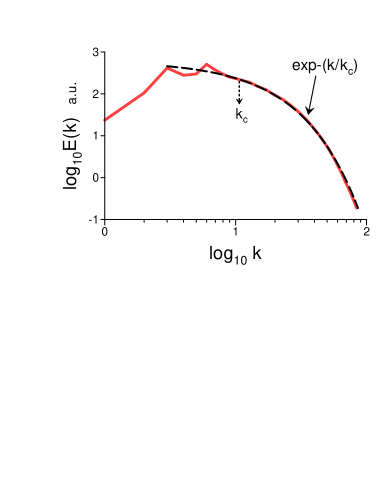
Figure 2: Magnetic energy spectrum at the saturation stage of a small-scale Hall MHD dynamo.

Deterministic chaos (at the onset of turbulence) is often characterized by the exponential power spectra (both temporal and spatial)fm -kds

$$E(f)\propto\exp-(f/f_{c})$$

and/or

$$E(k)\propto\exp-(k/k_{c})$$

where $f$ is frequency, $k$ is wavenumber.

Figure 1, for instance, shows (in the linear-log scales) the traces of average magnetic field power spectra measured in a laboratory experiment (the Large Plasma Device at UCLA) studying chaos in motions of magnetic flux ropes (magnetic structures with helical currents and magnetic fields) immersed in a magnetized helium plasma 002 . The magnetic flux ropes rotate about a central axis in a cylindrical vessel, writhe about each other, twist about themselves, and are kink unstable. Collisions between the magnetic ropes result in magnetic field lines reconnection.

According to Taylor’s “frozen in” hypothesis, the experimental spectrum shown in Fig. 1 should be interpreted as a wavenumber spectrum with $k\simeq 2\pi f/V_{0}$, where $V_{0}$ is the mean speed of the spatial magnetic structures passing the probe (cf., for instance, Refs. mm ,sbl and references therein). The dashed straight line is drawn through the upper curve in Fig. 1 to indicate the exponential spectrum Eq. (5) corresponding to the spatial deterministic chaos (the stretched exponential spectrum for the flux ropes at 110 V will be explained in the next Section).

In a recent paper Ref. hal the authors numerically simulated (DNS) a small-scale magnetohydrodynamic dynamo using the three-dimensional ‘incompressible’ Hall equations in the form:

$$\partial_{t}{\bf u}+({\bf u}\cdot\nabla){\bf u}=-\nabla\left(p+\frac{{\bf b}^{2}}{2}\right)+\left({\bf b}\cdot\nabla\right){\bf b}+\nu\nabla^{2}{\bf u}+{\bf f}$$

$$\partial_{t}{\bf b}=-\left({\bf u}\cdot{\bf\nabla}\right){\bf b}+\left({\bf b}\cdot\nabla\right){\bf u}+\eta\nabla^{2}\bf{b}+$$

$$+d_{i}\left({\bf j}\cdot{\bf\nabla}\right){\bf b}-d_{i}\left({\bf b}\cdot\nabla\right){\bf j}$$

$$\nabla\cdot{\bf u}=0,~{}~{}~{}{\bf\nabla}\cdot{\bf b}=0,$$

where ${\bf u}$ is the velocity field, $p$ is the kinetic pressure (normalized by the constant plasma density $\rho$), ${\bf f}$ is the hydrodynamic large-scale Taylor-Green external forcing: ${\bf f}\equiv f_{0}[\sin(k_{f}x)\cos(k_{f}y)\cos(k_{f}z){\hat{\bf x}}-\cos(k_{f}x)\sin(k_{f}y)\cos(k_{f}z){\hat{\bf y}}]$ (here $k_{f}=2$), $\eta$ and $\nu$ are the magnetic diffusivity and kinematic viscosity correspondingly, ${\bf b}={\bf B}/\sqrt{\mu_{0}\rho}$ is the normalized magnetic field, ${\bf j}=\nabla\times{\bf b}$, and $d_{i}$ is the ion inertial length.

The last two terms on the right-hand side of Eq. (7 ) represent the Hall effect. In the ideal Hall MHD ions are not already tied to the magnetic field due to the ions’ inertia, while the electrons still are. The ion inertial length $d_{i}$ corresponds to the spatial scale at which electrons and ions decouple.

Periodic boundary conditions have been used in the DNS for all spatial directions and a random seed magnetic field was introduced in a statistically stationary chaotic/turbulent motion of the fluid at small scales to initiate the small-scale magnetohydrodynamic dynamo. Magnetic Prandtl number $P_{m}=1$.

Figure 2 shows the magnetic energy spectrum at the saturation stage of the MHD dynamo. The spectral data were taken from Fig. 3 of the Ref. hal . The dashed curve indicates the exponential spectrum Eq. (5) (deterministic chaos). The dotted arrow indicates the position of the characteristic scale $k_{c}$.

In paper Ref. pg the transition from magnetohydrodynamics (large spatial scales) to kinetics (small spatial scales) in the solar wind was studied with emphasis on the effects related to the magnetic helicity (see also next Section).

Figure 3 shows the trace magnetic power spectrum measured at the Ulysses Northern Polar Pass ($R=2.36$ AU) in a fast (high-speed) solar wind. The spectral data were taken from Fig. 2 of the Ref. pg . The dashed vertical line indicates the frequency position (using Taylor’s “frozen-in” hypothesis) of the thermal ion gyroradius $\rho_{i}$. The dotted straight line in the log-log scales indicates the Kolmogorov-like power law $E(f)\propto f^{-5/3}$ (or according to Taylor’s “frozen-in” hypothesis $E(k)\propto k^{-5/3}$) for the large scales. The short-dash curve indicates correspondence to the exponential spectrum Eq. (5), i.e. to the deterministic chaos. The position of the characteristic frequency of the deterministic chaos $f_{c}$ is indicated by the dotted arrow (or according to Taylor’s “frozen-in” hypothesis the position of the characteristic wavenumber $k_{c}$) (cf Fig. 2).

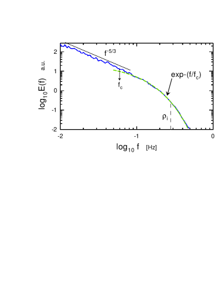
Figure 3: Trace magnetic power spectrum measured at the Ulysses Northern Polar Pass ($R=2.36$ AU).

III Distributed chaos dominated by magnetic helicity

At a sufficiently strong change of the parameters driving the magnetic field fluctuations dynamics the characteristic scale $k_{c}$ in Eq. (5) can become randomly fluctuating. Then to compute the magnetic power spectra one needs an ensemble averaging

$$E(k)\propto\int_{0}^{\infty}P(k_{c})\exp-(k/k_{c})dk_{c}$$

where a probability distribution $P(k_{c})$ characterizes the fluctuations of the characteristic scale $k_{c}$.

To find the probability distribution $P(k_{c})$ in the plasma dominated by the magnetic helicity one can use a scaling relationship between characteristic values of the magnetic field $B_{c}$ and $k_{c}$

$$B_{c}\propto|h_{m}|^{1/2}k_{c}^{1/2}$$

obtained with the dimensional considerations. If the $B_{c}$ has a normal distribution (Gaussian with zero mean my ), then $k_{c}$ has the chi-squared ($\chi^{2}$) distribution

$$P(k_{c})\propto k_{c}^{-1/2}\exp-(k_{c}/4k_{\beta})$$

where $k_{\beta}$ is a new characteristic constant.

Substituting Eq. (11) into Eq. (9) one obtains

$$E(k)\propto\exp-(k/k_{\beta})^{1/2}$$

This is the magnetic energy spectrum for a distributed chaos in the presumably non-dissipative range of scales dominated by the magnetic helicity.

In a special interesting case with global reflectional symmetry, the global (mean) magnetic helicity is identically equal to zero (or negligible). The point-wise magnetic helicity can be not identically equal to zero even in this case. Namely, the spontaneous breaking of the local reflectional symmetry (and related spontaneously generated local helical fluctuations) is an inherent property of the strongly chaotic/turbulent flows. The appearance of the blobs having non-zero blob’s kinetic/magnetic helicity can accompany this process (see, for instance, Refs. mt ,kerr -ber1 and references therein). Some of the magnetic blobs are bounded by the so-called magnetic surface where ${\bf b_{n}}\cdot{\bf n}=0$ (${\bf n}$ is a unit normal to the blob’s boundary). Sign-defined magnetic helicity of such a blob is an ideal invariant mt . Let us number the blobs and denote their helicity as $H_{j}^{\pm}$ depending on their sign ($j$ is the number of a blob):

$$H_{j}^{\pm}==\int_{V_{j}}({\bf a}({\bf x},t)\cdot{\bf b}({\bf x},t))~{}d{\bf x}$$

Then let us consider the ideal adiabatic invariant

$${\rm I^{\pm}}=\lim_{V\rightarrow\infty}\frac{1}{V}\sum_{j}[H_{j}^{\pm}]$$

where the summation in Eq. (13) is over the blobs with a certain sign only (‘+’ or ‘-’) and $V$ is the total spatial volume of the blobs considered for the sum.

Due to the global reflectional symmetry ${\rm I^{+}}\simeq-{\rm I^{-}}$. For the case of global reflectional symmetry the adiabatic invariant ${\rm I^{\pm}}$ Eq. (13) can replace $h_{m}$ in Eq. (10)

$$B_{c}\propto|{\rm I^{\pm}}|^{1/2}k_{c}^{1/2}$$

This replacement results in the same stretched exponential spectrum Eq. (12) for this case.

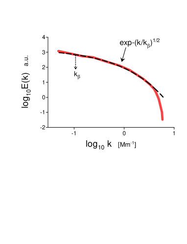
Figure 4: The spot and noise corrected magnetic power spectrum for the solar active region NOAA 8375.

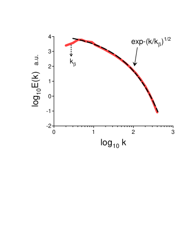
Figure 5: The DNS computed magnetic energy spectra for forced incompressible isotropic homogeneous MHD for $Re_{\lambda}=Re_{\lambda}^{m}=909$.

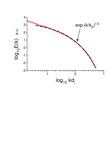
Figure 6: The DNS computed magnetic energy spectra for decaying compressible weakly anisotropic Hall MHD at the time of maximal dissipation.

The dashed curve is drawn through the middle curve in Fig. 1 to indicate the stretched exponential spectrum Eq. (12) corresponding to the spatially distributed chaos dominated by magnetic helicity. Since the experimental spatial domain is not enclosed completely by a magnetic flux surface the ${\bf a}$ is not gauge invariant. In this case, a gauge-invariant relative magnetic helicity with an appropriate reference magnetic field (the axial background magnetic field - constant in time and space outside the experimental vessel,) can be used instead bf ,jc ,dg .

It is well known that multiple flux ropes extend from the solar surface into the solar photosphere and corona. Coronal Mass Ejections can be triggered by the multiple flux ropes collisions amar .

In Ref. abr results of the space-based (SOHO/MDI) spectral measurements of the longitudinal magnetic fields in the solar active region NOAA 8375 (made on 4 November 1998) were reported. At the time of the measurements, the active region was located at the center of the solar disk. To avoid the strong contribution of the sunspot to the power spectrum the authors of the Ref. abr blocked out the sunspot. Figure 4 shows the spot and noise-corrected magnetic power spectrum (the spectral data were taken from Fig. 6b of the Ref. abr ). The dashed curve is drawn to indicate the stretched exponential spectrum Eq. (12) corresponding to the spatially distributed chaos dominated by magnetic helicity (cf Ref. ber2 ).

Magnetic ropes are routinely ejected from the Sun. These magnetic flux ropes can transport a large amount of magnetic helicity into the solar wind (see Section VI).

Let us start a comparison of the laboratory and solar data with the results of DNS of isotropic homogeneous pure magnetohydrodynamics (Eqs. (6-8) without the Hall terms) reported in a paper Ref. ae . The statistically stationary state with high $Re_{\lambda}=Re_{\lambda}^{m}=909$ was reached using the Taylor-Green forcing in a spatially periodic box.

Figure 5 shows the magnetic energy spectrum computed in this DNS (the spectral data were taken from Fig. 1 of the Ref. ae ). The dashed curve in Fig. 5 indicates the stretched exponential spectrum Eq. (12) corresponding to the spatially distributed chaos dominated by magnetic helicity (cf Figs. 1,4 and 12).

Figure 6 shows the magnetic energy spectrum computed in a DNS reported in a recent paper fer (the spectral data were taken from Fig. 6a of the Ref. fer ). In this DNS a freely decaying compressible isothermal case was studied in the frames of the Hall MHD with a weak background magnetic field. The DNS was performed in a cubic spatial box with periodic boundary conditions and with initial conditions consisting of a superposition of random phase harmonic modes. The energy of these modes in Fourier space was localized in a sphere $1<k<3$. The initial Mach number $M_{s}=0.25$ and $d_{i}=0.02L_{0}$ (where $L_{0}=2\pi$ is the size of the DNS cubic box). The spectrum was computed in the vicinity of the time when a maximal dissipation was reached.

The dashed curve in Fig. 6 indicates the stretched exponential spectrum Eq. (12) corresponding to the spatially distributed chaos dominated by magnetic helicity (cf Figs. 1,4).

IV Magneto-inertial range of scales

Conditions in the solar wind are significantly different from those in the solar atmosphere. The main difference is the high speed of the plasma moving away from the Sun. Therefore, a different phenomenology - magneto-inertial range (see Introduction) should be used for the solar wind. In this case, the estimate Eq. (10) should be replaced by

$$B_{c}\propto\varepsilon_{h}^{1/2}~{}\varepsilon^{1/6}~{}k_{c}^{1/6}$$

(cf the Corrsin-Obukhov phenomenology for the inertial-convective range my ).

If a significant mean magnetic field is present, then the energy dissipation rate $\varepsilon$ in Eq. (16) should be replaced by a more appropriate parameter $(\varepsilon\widetilde{B}_{0})$ (here $\widetilde{B}_{0}=B_{0}/\sqrt{\mu_{0}\rho}$ is the normalized mean magnetic field, having the same dimension as velocity ) ir . The dimensional considerations, in this case, result in

$$B_{c}\propto\varepsilon_{\hat{h}}^{1/2}~{}(\varepsilon\widetilde{B}_{0})^{1/8}k_{c}^{1/8}$$

with the modified magnetic helicity (see the Eq. (2)) dissipation rate $\varepsilon_{\hat{h}}$. However, the dimensional estimation Eq. (16) can be still valid for some cases even with a strong external magnetic field.

The estimates Eq. (16-17) can be generalized as

$$B_{c}\propto k_{c}^{\alpha}$$

Let us, following Eq. (12), seek the spectrum for the distributed chaos as a stretched exponential one

$$E(k)\propto\int_{0}^{\infty}P(k_{c})\exp-(k/k_{c})dk_{c}\propto\exp-(k/k_{\beta})^{\beta}$$

For large $k_{c}$ the probability distribution $P(k_{c})$ can be estimated from the Eq. (19) as jon

$$P(k_{c})\propto k_{c}^{-1+\beta/[2(1-\beta)]}~{}\exp(-\gamma k_{c}^{\beta/(1-\beta)})$$

Then, using some algebra, the relationship between the exponents $\beta$ and $\alpha$ can be readily obtained from the Eqs. (18) and (20) for the normally distributed $B_{c}$

$$\beta=\frac{2\alpha}{1+2\alpha}$$

Hence, for $\alpha=1/6$ (see Eq. (16))

$$E(k)=\exp-(k/k_{\beta})^{1/4}$$

and for $\alpha=1/8$ (see Eq. (17))

$$E(k)=\exp-(k/k_{\beta})^{1/5}$$

These are spatial magnetic power spectra in the magneto-inertial range of scales dominated by magnetic helicity.

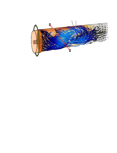
Figure 7: A sketch of the MHD (plasma gun) wind tunnel.

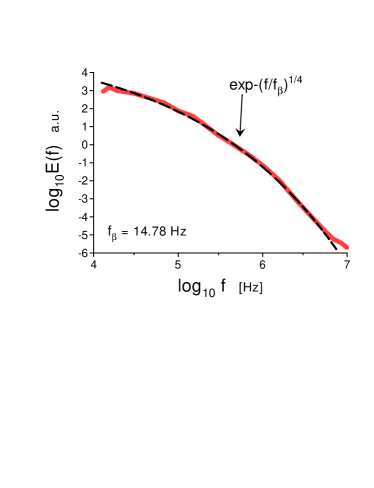
Figure 8: Ensemble averaged total magnetic energy spectrum measured in the MHD (plasma gun) wind tunnel experiment.

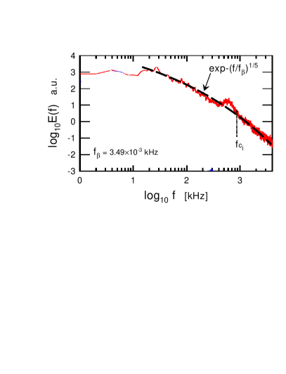
Figure 9: Power spectrum of the vertical component of the magnetic field measured within the plasma edge.

V Laboratory measurements vs DNS

V.1 Laboratory measurements

Figure 7 (adapted from the Ref. sbl ) shows a sketch of the MHD (plasma gun) wind tunnel. This experiment can imitate situations similar to those typical for solar wind. The blue lines in the figure show twisting of the magnetic field lines due to magnetic helicity conservation.

Figure 8 shows the ensemble-averaged total magnetic energy spectrum measured in the experiment. The spectral data were taken from Fig. 15a of the Ref. sbl . Taylor’s “frozen in” hypothesis can be used to transform the measured frequency spectrum to the more adequate in this case wavenumber spectrum. The dashed curve indicates correspondence to the stretched exponential spectrum Eq. (22).

In recent Ref. rich results of an experiment with local magnetic helicity injection into a toroidal system (a spherical tokamak startup) have been reported and the physical mechanisms converting the injected magnetic helicity into a large-scale current drive are experimentally studied. In this experiment, the intense electron current sources inject the magnetic helicity at the edge of a tokamak. Magnetic reconnections associated with the helicity-conserving instabilities convert the topology of the open field lines into a tokamak-like toroidal one.

Figure 9 shows the power spectrum of the vertical component of the magnetic field measured within the plasma edge. The spectral data were taken from Fig. 1 of the Ref. rich . The position of the local ion cyclotron frequency $f{\tiny c}_{i}$ is indicated by the dotted vertical line. The dashed curve indicates the stretched exponential spectrum Eq. (23).

V.2 MHD direct numerical simulations

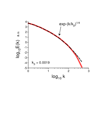
Figure 10: Magnetic energy spectra for the freely decaying MHD DNS with considerable mean magnetic helicity.

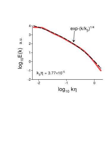
Figure 11: Magnetic energy spectrum for the forced MHD DNS with considerable mean magnetic helicity (here $\eta$ is the dissipation scale).

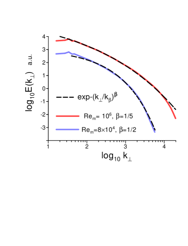
Figure 12: DNS computed field perpendicular magnetic energy spectra for two high values of magnetic Reynolds number: $Re_{m}=8\times 10^{4}$ and $Re_{m}=10^{6}$. The spectra are vertically shifted for clarity.

In a paper Ref. mpm results of direct numerical simulation of a freely decaying MHD flow (with ${\bf f}=0$ and without the Hall terms in the Eqs. (6-8)) with a superposition of random and deterministic (three ABC flows) initial conditions and considerable mean magnetic helicity were reported. The Kelvin-Helmholtz instabilities with rolling up of current and vorticity sheets were observed at a high Reynolds number ($Re=10100$).

Figure 10 shows magnetic energy spectra for $t=1.6$ in terms of the DNS (the spectral data were taken from Fig. 2b of the Ref. mpm ). The dashed curve indicates the stretched exponential spectrum Eq. (22).

In a paper Ref. yos a direct numerical simulation using the forced MHD equations was performed in a 3D spatial box (periodic boundary conditions). The initial fields were randomly generated with kinetic and magnetic energies equal to 0.5 (in the terms of the Ref. yos ). The initial mean cross helicity was taken almost zero, while the initial mean (normalized) magnetic helicity was rather considerable - 0.515 (at the statistically stationary state the normalized mean magnetic helicity was 0.655). The large-scale random forcing ${\bf f}$ was concentrated in the wavenumber range $1<k<2.5$. The magnetic Prandtl number $Pr_{m}=1$, the Taylor-Reynolds number $Re_{\lambda}=150$ and the magnetic Reynolds number $Re_{\lambda}^{(m)}=306$.

Figure 11 shows the magnetic energy spectrum computed for the statistically stationary state using a wavelet method (here $\eta$ is the dissipation scale). The spectral data were taken from Fig. 1 of the Ref. yos . The dashed curve indicates correspondence to the stretched exponential spectrum Eq. (22) .

In a recent paper Ref. dong the MHD equations

$$\partial_{t}\rho+\nabla\cdot(\rho{\bf{u}})=0$$

$$\partial_{t}(\rho{\bf{u}})+\nabla\cdot(\rho{\bf{uu}})=-\nabla\left(p+B^{2}/2\right)+\nabla\cdot({\bf{BB}})+\nu{\nabla^{2}}(\rho{\bf{u}})$$

$$\partial_{t}p+\nabla\cdot(p{\bf{u}})=(\gamma-1)\left({-p\nabla\cdot{\bf{u}}+\eta{\bf{J}}^{2}}\right)$$

$$\partial_{t}{\bf{B}}=\nabla\times({\bf{u}}\times{\bf{B}}-\eta{\bf{J}})$$

(where $\gamma$ denotes the adiabatic index) were numerically solved for a very high magnetic Reynolds number $Re_{m}=10^{6}$. The equations Eqs. (24-27) were solved in a periodic spatial box elongated ($1\times 1\times 2$) along the direction of an imposed strong mean magnetic field ${\bf B_{0}}$. The dynamics was initialized by uncorrelated, equipartitioned magnetic and velocity fields.

Figure 12 shows the field perpendicular magnetic energy spectra computed in this DNS for two values of $Re_{m}=10^{6}$ and $Re_{m}=8\times 10^{4}$. The spectral data were taken from Fig. 2 of the Ref. dong . The dashed curves indicate correspondence to the stretched exponential spectra: Eq. (12) for $Re_{m}=8\times 10^{4}$, and Eq. (23) for $Re_{m}=10^{6}$.

It should be noted that for $Re_{m}>10^{5}$ the authors of the DNS observed a tearing instability of the elongated current sheets resulting in the formation of the small magnetic flux ropes (plasmoids). For $Re_{m}=8\times 10^{4}$ the flux ropes were practically absent.

V.3 Electron magnetohydrodynamics (EMHD)

There are different theoretical (numerical) models for the transitional range between large-scale magnetohydrodynamics and small-scale kinetics (see, for instance, Refs. sch1 ,sch and references therein). If for the MHD scales one can treat the plasma as a single conducting fluid, for the transitional region a simple two-fluid model - electron magnetohydrodynamics (EMHD), can be applied as a first approximation. This model is rather appropriate for the cases dominated by the magnetic helicity cho . It is assumed in the EMHD that ions provide only a motionless charge background for the fast electron flows which carry current and determine the dynamics of the magnetic field ${\bf B}$

$${\bf u}_{e}=-\frac{{\bf J}}{n_{e}e}=-\frac{c}{4\pi n_{e}e}[\nabla\times{\bf B}]$$

where ${\bf J}$ is the electric current density, ${\bf u_{e}}$ is the electron velocity, $n_{e}$ is the electron number density kin .

Substitution of the Eq. (28) into the equation

$$\frac{\partial{\bf B}}{\partial t}=\nabla\times[{\bf u}_{e}\times{\bf B}]+\eta\nabla^{2}{\bf B}$$

provides an equation describing the dynamics of the magnetic field in the incompressible EMHD

$$\frac{\partial{\bf B}}{\partial t}=-\frac{c}{4\pi n_{e}e}\nabla\times[(\nabla\times{\bf B})\times{\bf B}]+\eta\nabla^{2}{\bf B}$$

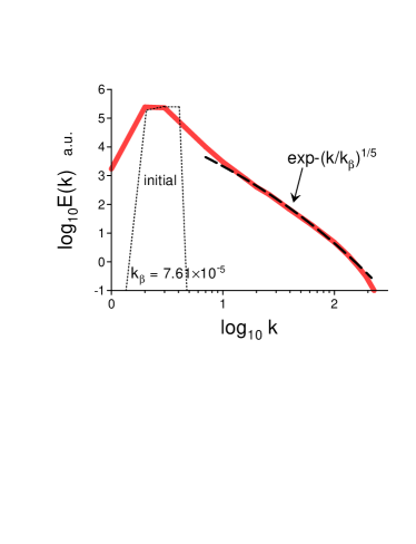
Figure 13: Magnetic energy spectrum of the freely decaying positive EMHD wave packets at $t=0.6$.

Figure 14: As in Fig. 13 but for negative EMHD wave packets.

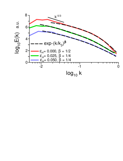
Figure 15: Magnetic magnetic energy spectra for the decaying isotropic MHD and Hall MHD for different values of the Hall parameter. The spectra are vertically shifted for clarity.

It should be noted that magnetic helicity for the EMHD is conserved in the ideal case similar to the MHD sch1 . Unlike the MHD Alfvèn waves the EMHD waves are helical and carry a nonzero magnetic helicity. Also, the EMHD waves are dispersive and can interact with each other. In a strong imposed magnetic field the direction of propagation of the EMHD wave packets is either parallel or antiparallel to the magnetic field lines. One can speak about ‘positive’ and ‘negative’ wave packets in respect to the sign of the magnetic helicity carried by the wave packets.

In the Ref. cho the Eq. (30) was solved numerically in a periodic box for the decaying case with an imposed uniform magnetic filed ${\bf B}_{0}$ (so that ${\bf B}={\bf B}_{0}+{\bf b}$). Figure 13 shows the power spectrum of magnetic energy of the freely decaying positive EMHD wave packets obtained with this DNS (the spectral data were taken from Fig. 4 of the Ref. cho for $t=0.6$ in terms of the Ref. cho ). The dotted lines show the initial energy spectrum (only positive waves were present in the DNS at $t=0$). The dashed curve indicates the stretched exponential spectrum Eq. (23).

The EMHD wave packets moving in one direction interact with each other and, therefore, can generate counterpropagating waves. Figure 14 shows the power spectrum of magnetic energy of the freely decaying negative EMHD wave packets obtained with this DNS (the spectral data were taken from Fig. 4 of the Ref. cho for $t=0.6$). The dashed curve indicates the stretched exponential spectrum Eq. (22).

V.4 Hall magnehydrodynamics

In a paper Ref. ma results of direct numerical simulations of the decaying, incompressible, homogeneous, isotropic MHD and Hall MHD were reported. The DNS were performed in a periodic spatial cube with random phase initial conditions and initial energy spectrum

$$E(k)\propto k^{4}\exp-(k^{2}/k_{0}^{2})$$

for both the velocity and magnetic field (here $k_{0}=2$). The initial kinetic and magnetic energies were approximately the same.

Figure 15 shows the DNS computed magnetic energy spectra for the decaying isotropic MHD and Hall MHD for different values of the Hall parameter $\epsilon_{H}=d_{i}/L_{0}$ at $t=2.4$ in the DNS terms. The spectral data were taken from Fig. 2b of the Ref. ma . The dashed curves indicate the stretched exponential spectra: Eq. (12) for $\epsilon_{H}=0$ (MHD), and Eq. (22) for $\epsilon_{H}=0.025$, and $\epsilon_{H}=0.050$ for Hall MHD.

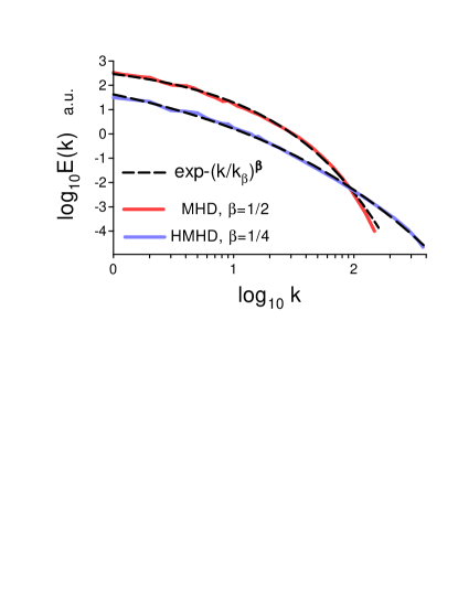
Figure 16: Magnetic magnetic energy spectra for the weakly incompressible decaying isotropic MHD and Hall MHD. The spectra are vertically shifted for clarity.

In a recent paper Ref. fold results of a Lattice Boltzmann numerical simulation of a weakly compressible MHD and Hall MHD were reported. The simulations were performed in a periodic cubic lattice and were initialized with the Orszag-Tang vortex.

Figure 16 shows the magnetic energy spectra computed at the peak of magnetic dissipation both for the MHD case and for the Hall MHD case ($\epsilon_{H}=0.015$, $Re=6000$, $Pr_{m}=1$). The spectral data were taken from Fig. 11 of the Ref. fold for the MHD case and from Fig. 14 of the Ref. fold for the Hall MHD case.

The dashed curves indicate the stretched exponential spectra: Eq. (12) for the MHD case, and Eq. (22) for the Hall MHD case.

V.5 A fully kinetic numerical simulation

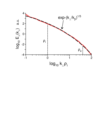
Figure 17: Perpendicular magnetic energy spectrum vs $k_{\perp}\rho_{i}$ ($\rho_{i}$ and $\rho_{e}$ are ion and electron gyroradius respectively) for a fully kinetic numerical simulation.

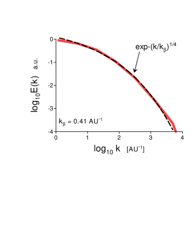
Figure 18: Total magnetic energy spectrum for the fast solar wind at $2.8<R<4.5$AU (Ulysses, 1993-1996yy).

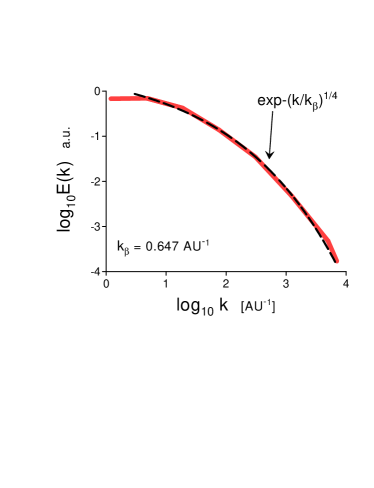
Figure 19: The same as in Fig. 18 but at $1.5<R<2.8$ AU.

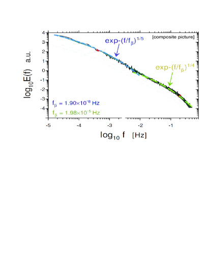
Figure 20: Total magnetic energy spectrum for the fast solar wind at at $R=1.4$AU (Ulysses).

In a paper Ref. thd results of a gyrokinetic numerical simulation were reported. In this simulation the authors numerically solved the electromagnetic gyroaveraged Vlasov–Maxwell equations for electrons and protons as well as for the component of the vector potential ${\bf A}$ parallel to the equilibrium magnetic field ${\bf B}_{0}$, for the parallel perturbation of the magnetic field, and the electrostatic potential. The equilibrium distribution functions for protons and electrons are Maxwellian. A conservative collision operator was linearized and gyroaveraged. The simulation was driven by an oscillating Langevin antenna which was coupled to the component of the vector potential parallel to ${\bf B}_{0}$. The parameters of the plasma were chosen as follows: $\beta_{i}=1$, $m_{i}/m_{e}=1836$, and $Ti/Te=1$. The simulation was performed in a periodic three-dimensional spatial domain elongated along the uniform magnetic field ${\bf B}_{0}$.

Figure 17 shows the perpendicular magnetic energy spectrum vs $k_{\perp}\rho_{i}$ ($\rho_{i}$ and $\rho_{e}$ are ion and electron gyroradius respectively). The spectral data were taken from Fig. 1 of the Ref. thd . The dashed curve indicates the stretched exponential spectrum Eq. (23). The short-dashed vertical lines are drawn to indicate the positions of the gyroradii $\rho_{i}$ and $\rho_{e}$.

VI Solar wind

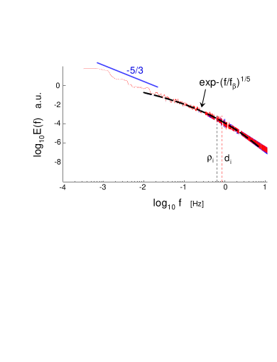
Figure 21: Power spectrum of magnetic field fluctuations for the fast solar wind at $R=1$AU (ARTEMIS-P2).

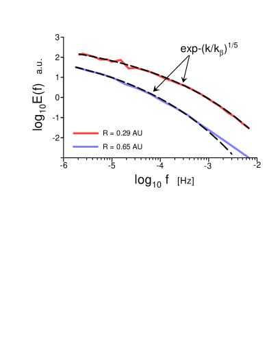
Figure 22: Total magnetic energy spectrum for the fast solar wind at $R=0.65$AU and $R=0.29$AU (Helios 2).

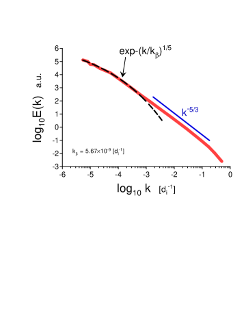
Figure 23: Magnetic energy spectrum computed from the auto-correlation of the magnetic field fluctuations measured at $R=0.16$AU (near Parker Solar Probe first perihelion).

Solar wind is characterized by a wide variety of physical conditions. Distance from the Sun, fast or slow wind, etc. determine these physical conditions. Spacecraft measurements provide us with good-quality data observed in this unique natural laboratory.

Figure 18, for instance, shows the total magnetic energy spectrum calculated using measurements made by Ulysses mission for the 1993-1996yy period at the high heliolatitudes and in the fast solar wind. The spectral data were taken from Fig. 3 of the Ref. bran for $2.8<R<4.5$ astronomical units (AU), where $R$ is the distance from the Sun. The spectral data were rescaled by a factor $4\pi R^{2}$ before averaging. Figure 19 shows the analogous spectrum for $1.5<R<2.8$ AU (the spectral data were taken from the Fig. 3 of the Ref. bran ). The wavenumber spectra were obtained using Taylor’s “frozen in” hypothesis. The dashed curves indicate correspondence to the stretched exponential spectrum Eq. (22).

Figure 20 shows the total magnetic energy spectrum for the fast solar wind at $R=1.4$AU computed using measurements made by the Ulysses mission. The spectral data were taken from Fig. 1 of the Ref. tbt (see also Refs. bc ,bt ). The dashed curves indicate correspondence to the stretched exponential spectrum Eq. (23) for the large spatial scales (small frequencies in the figure) and to the stretched exponential spectrum Eq. (22) for the small spatial scales (large frequencies in the figure).

Figure 21 shows the power spectrum of magnetic field fluctuations measured at $R=1$AU by ARTEMIS-P2 spacecraft. The spectral data were taken from Fig. 1 of Ref. chen . The dashed curve indicates correspondence to the stretched exponential spectrum Eq. (23). The ion gyroradius $\rho_{i}$ and ion inertial length $d_{i}$ are indicated in Fig. 21 by the vertical dotted lines. The appearance of the Kolmogorov-like power law spectrum at large scales is indicated by the straight solid line with the slope -5/3 (cf. Ref. bs ).

Space probe Helios 2 observed solar wind in the ecliptic and much closer to the Sun rosen . Figure 22 shows the total magnetic energy spectrum for the fast solar wind at $R=0.65$AU and $R=0.29$AU. The spectral data were taken from Fig. 1 of Ref. tbt (see also Refs. bc ,bt ). The dashed curves indicate correspondence to the stretched exponential spectrum Eq. (23).

The NASA Parker Solar Probe studies the deeper inner heliosphere fox . Figure 23 shows the magnetic energy spectrum computed from the auto-correlation of the magnetic field fluctuations measured at $R=0.16$AU (near Parker Solar Probe’s first perihelion). The spectral data were taken from Fig. 1b of the Ref. gue . Taylor’s hypothesis was used to convert the time lags $\tau$ into the wavenumbers (in this figure $k=1/V_{0}\tau$, where $V_{0}$ is the mean solar wind speed), and the wavenumber was taken in the units of the inverse ion inertial length $1/d_{i}$. The dashed curve indicates correspondence to the stretched exponential spectrum Eq. (23) for the large spatial scales. For the small spatial scales, a Kolmogorov-like spectrum was observed (indicated by the straight line in the log-log scales).

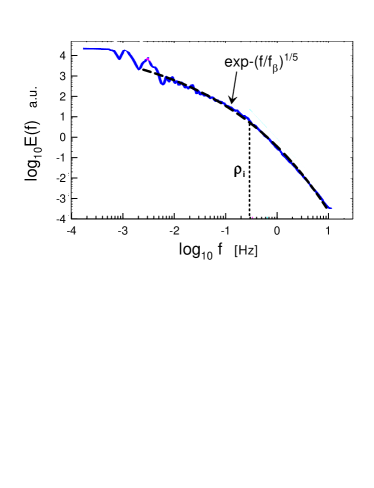
Figure 24: Power spectrum of magnetic fluctuations in the magnetosheath near the bow shock. Cluster spacecraft measurements.

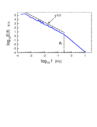
Figure 25: Power spectrum of magnetic fluctuations in the magnetosheath near the magnetopause (toward the flank region). Cluster spacecraft measurements.

VII In the Earth’s and Saturn’s magnetosphere

VII.1 Magnetosheath

Let us start with the Earth’s magnetosheath, i.e. the area of the magnetosphere bounded by the magnetopause and the bow shock.

Figure 24 shows the power spectrum of magnetic fluctuations in the magnetosheath near the bow shock, whereas Fig. 25 shows the power spectrum of magnetic fluctuations in the magnetosheath near the magnetopause (toward the flank region). The spectral data were taken from Fig. 1 of a paper Ref. huang2 (the raw data were obtained by the Cluster mission, see Ref. huang2 for more details and references). The dashed curve in Fig. 24 indicates the spectral law Eq. (23), whereas the dashed straight line in Fig. 25 indicates the Kolmogorov-like spectral law (the authors of the Ref. huang2 argued that the nature of this Kolmogov-like spectral law is still unclear). The ion gyroradius $\rho_{i}$ is indicated by the vertical dotted lines.

Figure 26 shows the power spectrum of magnetic fluctuations in the magnetosheath computed for the data obtained by the Magnetospheric Multi-Scale spacecraft (the spectral data were taken from Fig. 1 of the Ref. par ). Taylor’s hypothesis was used to transform the frequency spectrum into the wavenumber one (the authors of the Ref. par provide certain arguments supporting the application of the Taylor hypothesis to this case). The spacecraft was approximately at 14.8 $R_{E}$ ($R_{E}$ is the Earth’s radius). The dashed curve in Fig. 26 indicates the spectral law Eq. (23).

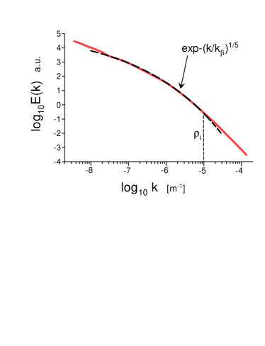
Figure 26: Power spectrum of magnetic fluctuations in the magnetosheath at 14.8 $R_{E}$ (Magnetospheric Multi-Scale spacecraft).

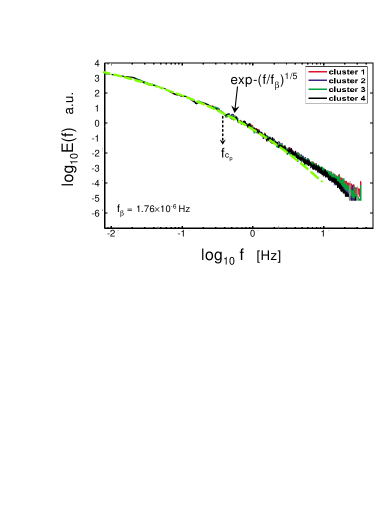
Figure 27: Power spectrum of the magnetic field measured in the magnetospheric reconnection jet (Cluster mission).

VII.2 Reconnection jet in the plasma sheet of the Earth’s magnetosphere

In a paper Ref. huang results of measurements with four Cluster spacecraft in the plasma sheet of the Earth’s magnetosphere were reported. The event under consideration was a high-speed reconnection jet with a moderate mean (guide) magnetic field (see Introduction). Based on the observations the authors of the Ref. huang argued that the observed turbulence was strongly driven by the reconnection jet (cf Ref. alaoui ).

Figure 27 shows the power spectrum of the magnetic field measured during the event. The spectral data were taken from Fig. 1 of the Ref. huang . The position of the proton cyclotron frequency $f{\tiny c}_{p}$ is indicated by the vertical dotted arrow. The dashed curve indicates the stretched exponential spectrum Eq. (23) (cf Fig. 9 and corresponding comments).

VII.3 Kelvin-Helmholtz vortices at the Earth’s magnetopause

The Kelvin-Helmholtz vortices (or the flow shear-driven Kelvin-Helmholtz instability) at Earth’s magnetopause can be a significant factor for the transport of momentum and mass from the solar wind environment into Earth’s magnetosphere (see, for instance, Ref. has and references therein).

Figure 28: Power spectrum of a magnetic field component computed in the numerical simulation and corresponding to the magnetic field component normal to the nominal magnetopause in the MMS observations.

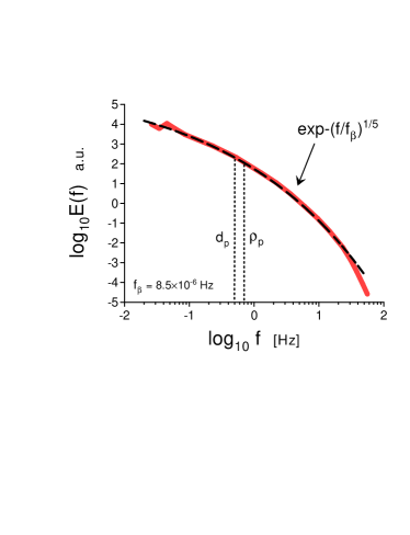
Figure 29: Power spectrum of the magnetic field component normal to the nominal magnetopause measured by the MMS for the Kelvin-Helmholtz active period.

In recent Ref. nak results of a 3D kinetic simulation of the Kelvin-Helmholtz instability, with the conditions relevant to the Magnetospheric Multiscale spacecraft (MMS) observations in the Earth’s magnetopause has , were reported. Figure 28 shows the power spectrum of a magnetic field component computed in the numerical simulation and corresponding to the magnetic field component normal to the nominal magnetopause in the MMS observations. The spectral data were taken from Fig. 4b of the Ref. has . The $\lambda_{KH}$ denotes the most unstable Kelvin-Helmholtz instability wavelength, and the ion gyroradius $\rho_{i}$ and ion inertial length $d_{i}$ are indicated in Fig. 28 by the vertical dotted lines. The dashed curve indicates the stretched exponential spectrum Eq. (22).

In the Ref. has results of measurements produced by the Magnetospheric Multiscale spacecraft (MMS) in the Kelvin-Helmholtz vortices at the magnetopause were reported. Figure 29 shows the corresponding power spectrum of the magnetic field component perpendicular to the mean magnetic field and normal to the nominal magnetopause for the Kelvin-Helmholtz active period. The spectral data were taken from Fig. 3a of the Ref. has . The proton gyroradius $\rho_{p}$ and proton inertial length $d_{p}$ are indicated in Fig. 29 by the vertical dotted lines. The dashed curve indicates the stretched exponential spectrum Eq. (23).

It is interesting that for both the numerical simulation Fig. 28 and the real magnetospheric measurements Fig. 29 the magnetic helicity-dominated spectral laws Eq. (22) and Eq. (23) were observed. For the real measurements, however, a significant role of the background magnetic field was apparent.

VII.4 Saturn’s magnetosphere

The physical conditions in Saturn’s magnetosphere are rather different from those in the solar wind and Earth’s magnetosphere. The background magnetic field in this case is strong whereas the magnetic field fluctuations are rather weak. While the Earth’s magnetosphere is mainly driven by the surrounding solar wind Saturn’s magnetosphere is mainly driven by the planet’s rotation. For the middle magnetosphere $6R_{S}<r<15R_{S}$ (which will be considered in this subsection) a ring current and a flux tube interchange also play a significant role. Due to the fast rotation of the planet, the magnetospheric plasma is mainly concentrated in a plasma sheet located in the equatorial plane. Considering these circumstances it is interesting whether the above-discussed magnetic helicity-determined spectral laws will also take place in Saturn’s magnetosphere as well.

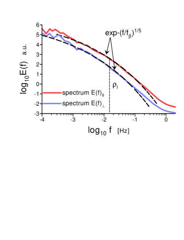
Figure 30: Power spectra of the magnetic field fluctuations components corresponding to the planetary ring current $r>9R_{S}$ (Cassini mission).

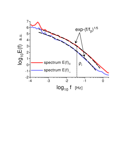
Figure 31: Power spectra of the magnetic field fluctuations components corresponding to the plasma dynamics throughout the time of isolated flux tube interchanges (Cassini mission).

In a paper Ref. psa results of a statistical analysis of the measurements produced by the Cassini spacecraft in Saturn’s middle magnetosphere (inside the plasma sheet) were reported. Figure 30 shows the power spectra of the magnetic field fluctuations components parallel and perpendicular to the mean magnetic field. The spectral data were taken from Fig. 6a of the Ref. psa (the inbound leg of the Cassini spacecraft’s second orbit). The data correspond to the planetary ring current $r>9R_{S}$. The dashed curves indicate the stretched exponential spectrum Eq. (23).

Figure 31 also shows the power spectra of the magnetic field fluctuations components parallel and perpendicular to the mean magnetic field. The spectral data were taken from Fig. 6c of the Ref. psa (the inbound leg of the Cassini spacecraft’s second orbit). The data correspond to the plasma dynamics throughout the time of isolated flux tube interchanges. The dashed curves indicate the stretched exponential spectrum Eq. (23).

Despite significant differences in the physical conditions of Saturn’s magnetosphere from those in the solar wind and Earth’s magnetosphere, the magnetic helicity-determined spectral law Eq. (23) is valid there as well.

VIII Conclusions

The variability of the spectral laws of the magnetic field fluctuations in the space plasmas is determined by the variability of the physical conditions in the solar, solar wind, and planet magnetosphere plasmas. An additional source of variability is the differences between the large-scale (MHD) and small-scale (kinetic) dynamics. Therefore, the existence of certain universality in the abundant observational, experimental, and DNS data can be useful in understanding the underlying physics. A significant help in the search of this universality can provide the fundamental ideal invariants such as energy and magnetic helicity.

It is shown in the present paper that the magnetic helicity-determined spectral laws Eqs. (12), (22), and (23) can provide a reasonable description for a rather wide class of data in the frames of the Kolmogorov-Iroshnikov phenomenology based on the notion of distributed chaos. This approach allows also the description of the transitional range of scales between MHD and kinetics which makes it applicable for the space plasmas where this transition is omnipresent.

Comparing the spectral behavior in the solar wind for different distances from the Sun one can conclude that in the near Sun heliosphere, the role of the background magnetic field becomes more prominent Eq. (23) than for the larger distances from the Sun Eq. (22). The transitional distance for this phenomenon seems to be near the value 1.4 AU Fig. 20.

In the planets’ magnetosphere, the spectral law Eq. (23) is also prevailing, i.e. the role of the background magnetic field is generally significant there as well.

IX Acknowledgments

I thank H.K. Moffatt for drawing my attention to the paper Ref. moff2 . I also thank R. Grappin and J.V. Shebalin for discussions.

References

- (1) H.K. Moffatt and A. Tsinober, Annu. Rev. Fluid Mech., 24, 281 (1992)
- (2) A.A. Schekochihin, S.C. Cowley, W. Dorland, G.W.Hammett, G.G.Howes, E. Quataert and T. Tatsuno, Astrophys. J. Suppl. Ser., 182, 310 (2009).
- (3) J.M. Polygiannakis and X. Moussas, Plasma Phys. Control. Fusion, 43 195 (2001)
- (4) W.H. Matthaeus and M.L. Goldstein, J. Geophys. Res., 87, 6011 (1982).
- (5) J.V. Shebalin, Phys. Plasmas, 20, 102305 (2013).
- (6) A.S. Monin, A.M. Yaglom, Statistical Fluid Mechanics, Vol. II: Mechanics of Turbulence (Dover Pub. NY, 2007).
- (7) U. Frisch and R. Morf, Phys. Rev., 23, 2673 (1981).
- (8) A. Brandstater and H. L. Swinney, Phys. Rev. A 35, 2207 (1987).
- (9) J. E. Maggs and G. J. Morales, Phys. Rev. Lett. 107, 185003 (2011); Phys. Rev. E 86, 015401(R) (2012); Plasma Phys. Control. Fusion 54 124041 (2012).
- (10) S. Khurshid, D.A. Donzis, and K.R. Sreenivasan, Phys. Rev. Fluids, 3, 082601(R) (2018).
- (11) W. Gekelman et al., Plasma Phys. Control. Fusion, 56, 064002 (2014).
- (12) D.A. Schaffner, M.R. Brown, and V.S. Lukin, ApJ, 790, 126 (2014).
- (13) A. Halder, S. Banerjee, A.G. Chatterjee, and M.K. Sharma, Phys. Rev. Fluids 8, 053701, (2023).
- (14) J.J. Podesta and S.P. Gary, ApJ, 734, 15 (2011).
- (15) R.M. Kerr, In: Elementary Vortices and Coherent Structures, Proceedings of the IUTAM Symposium Kyoto, 1-8 (2004)
- (16) D.D. Holm, R.M. Kerr, Physics of Fluids, 19, 025101 (2007)
- (17) A.A. Schekochihin, J. Plasma Phys., 88 (5), 155880501 (2022)
- (18) H.K. Moffatt, J . Fluid Mech., 35, 117 (1969)
- (19) H.K. Moffatt, J . Fluid Mech., 159, 359 (1985)
- (20) E. Levich and A. Tsinober, Phys. Lett. A 93, 293 (1983)
- (21) A. Bershadskii, E. Kit, A. Tsinober, Proc. R. Soc. Lond. A, 441, 147 (1993)
- (22) A. Bershadskii, arXiv:2305.05554 (2023)
- (23) M.A. Berger and G.N. Field, J. Fluid Mech., 147, 133 (1984).
- (24) T.H. Jensen and M.S. Chu, Phys. Fluids, 27, 2881 (1984).
- (25) T. DeHaas, and W. Gekelman, Phys. Plasmas, 24, 072108 (2017).
- (26) T. Amari, J.F. Luciani, J.J. Aly, Z. Mikic, and J. Linker, ApJ. 595, 1231 (2003).
- (27) V. Abramenko, V. Yurchyshyn, H. Wang, P.R Goode, Solar Physics, 201, 225 (2001).
- (28) A. Bershadskii, Res. Notes AAS, 4, 10 (2020).
- (29) H. Aluie and G.L. Eyink, Phys. Rev. Lett., 104, 081101 (2010)
- (30) R. Ferrand, F. Sahraoui, S. Galtier N. Andrés, P. Mininni, and P. Dmitruk, ApJ, 927, 205 (2022)
- (31) R.S. Iroshnikov, Astronomicheskii Zhurnal, 40, 742 (1963) (English translation in Soviet Astronomy 7, 566 (1964)).
- (32) D.C. Johnston, Phys. Rev. B, 74, 184430 (2006).
- (33) N.J. Richner, G.M. Bodner, M.W. Bongard , R.J. Fonck , M.D. Nornberg , and J.A. Reusch, Phys. Rev. Lett., 128, 105001 (2022).
- (34) P.D. Mininni, A.G. Pouquet, and D.C. Montgomery, Phys. Rev. Lett., 97, 244503 (2006).
- (35) K. Yoshimatsu, K. Schneider, N. Okamoto, Y. Kawahara, and M. Farge, Phys. Plasmas, 18, 092304 (2011).
- (36) C. Dong, L. Wang, Y.M. Huang, L. Comisso, T.A. Sandstrom, and A. Bhattacharjee, Sci. Adv., 8 (49), eabn7627 (2022).
- (37) J. Cho and H. Kim, J. Geophys. Res. Space Physics,, 121, 6157 (2016).
- (38) A.S. Kingsep, K V. Chukbar, and V.V. Yankov, Rev. Plasma Phys., 16, (1990).
- (39) H. Miura and K. Araki, Phys. Plasmas, 21, 072313 (2014).
- (40) R. Foldes, E. Leveque, R. Marino, E. Pietropaolo et al., J. Plasma Phys., 89, 905890413 (2023).
- (41) J.M. TenBarge, G.G. Howes, and W. Dorland, ApJ, 774, 139 (2013).
- (42) A. Brandenburg, K. Subramanian, A. Balogh, M.L. Goldstein, ApJ, 734, 9 (2011).
- (43) D. Telloni, R. Bruno, and L. Trenchi, ApJ, 805, 46 (2015).
- (44) R. Bruno, and V. Carbone, LRSP, 10, 2 (2013).
- (45) R. Bruno, and L. Trenchi, ApJL, 787, L24 (2014).
- (46) C.H.K. Chen, S. Boldyrev, Q. Xia, and J.C. Perez, Phys. Rev. Lett., 110, 225002 (2013).
- (47) A. Bershadskii, K.R. Sreenivasan, Phys. Rev. Lett., 93, 064501 (2004).
- (48) H. Rosenbauer, R. Schwenn, E. Marsch, E., et al., J. Geophysics Zeitschrift Geophysik, 42, 561 (1977)
- (49) N.J Fox, M.C. Velli, S.D. Bale, R. Decker, A. Driesman, R.A. Howard, J.C. Kasper, J. Kinnison, M. Kusterer, D. Lario, D.; et al., Space Sci. Rev., 204, 7 (2016).
- (50) M.E. Cuesta, T.N. Parashar, R. Chhiber, and W.H. Matthaeus, arXiv:2202.01874 (2022).
- (51) S.Y. Huang, L.Z. Hadid, F. Sahraou, Z. G. Yuan, and X. H. Deng, ApJ, Letters, 836, L10 (2017).
- (52) T. N. Parashar, A. Chasapis, Riddhi Bandyopadhyay, et al., Phys. Rev. Lett., 121, 265101 (2018).
- (53) S.Y. Huang, M. Zhou, and F. Sahraoui et al., Geophys. Res. Lett., 39, L11104 (2012).
- (54) M. El-Alaoui, M. Ashour-Abdalla, R L. Richard, M.L. Goldstein, J.M. Weygand, and R.J. Walker, J. Geophys. Res., 115, A12236 (2010).
- (55) H. Hasegawa, T.K.M. Nakamura, D.J. Gershman, Y. Nariyuki, A.F. Vinas, et al., JGR: Space Physics, 125, e2019JA027595 (2020).
- (56) T.K.M. Nakamura, The Earth’s low-latitude boundary layer, in Magnetospheres in the Solar System (eds. R. Maggiolo, N. Andre, H. Hasegawa, and D. Welling), John Wiley & Sons, Inc, Hoboken, NJ (2020).
- (57) M. von Papen, J. Saur, and O. Alexandrova, J. Geophys. Res. Space Physics, 119, 2797 (2014).