Jacobian Norm for Unsupervised Source-Free Domain Adaptation

Abstract

Unsupervised Source (data) Free domain adaptation (USFDA) aims to transfer knowledge from a well-trained source model to a related but unlabeled target domain. In such a scenario, all conventional adaptation methods that require source data fail. To combat this challenge, existing USFDAs turn to transfer knowledge by aligning the target feature to the latent distribution hidden in the source model. However, such information is naturally limited. Thus, the alignment in such a scenario is not only difficult but also insufficient, which degrades the target generalization performance. To relieve this dilemma in current USFDAs, we are motivated to explore a new perspective to boost their performance. For this purpose and gaining necessary insight, we look back upon the origin of the domain adaptation and first theoretically derive a new-brand target generalization error bound based on the model smoothness. Then, following the theoretical insight, a general and model-smoothness-guided Jacobian norm (JN) regularizer is designed and imposed on the target domain to mitigate this dilemma. Extensive experiments are conducted to validate its effectiveness. In its implementation, just with a few lines of codes added to the existing USFDAs, we achieve superior results on various benchmark datasets.

I Introduction

Deep neural networks have achieved remarkable success in various multi-media applications, where sufficiently large-scale and well-labeled data are present. However, manually labeling sufficient data is often time-consuming and labor-exhaustive, thus hard to meet the demand of rapid growth of the multi-media steaming or the content sharing applications [1]. To address it, unsupervised domain adaptation (UDA) is becoming an increasingly attractive research topic in the multi-media community [2, 3, 4, 5, 6]. Specifically, by leveraging the discriminative knowledge from readily available and labeled source domains, UDA aims to establish a desired prediction model for the unlabeled target domain, which significantly relieves the burden of annotating magnanimous data. In the past few years, UDA has achieved several impressive results on various multi-media applications such as image recognition [7, 8], semantic segmentation [9], text classification [10], recommendation [11] and action recognition [12].

Currently, a series of theoretical results have been presented to guide the solution for addressing UDA [13, 14], which illustrates that the target risk is bounded by the between-domain discrepancy. Motivated by these theoretical results, domain alignment comes to the dominant strategy for solving domain adaptation [2], whose goal is to alleviate the between-domain discrepancy, so that the learned source model can be naturally adapted to the target domain. Specifically, these methods can be categorized into the sample alignment or the feature alignment [2]. In particular, the sample alignment focuses on mitigating the domain shifts by the importance-weighting of samples [15, 16, 17]. In contrast, the feature alignment attempts to learn a domain invariant feature or representation to alleviate the domain discrepancies by kernel matching [18], adversarial learning [19], prototype matching [5], optimal transport [20] and image reconstruction [21].

In practice, almost all existing UDA approaches require to access both raw source and target data while learning to adapt. Unfortunately, due to the cost of storage or the protection of private information, in reality, the source data is often not at hand. In light of this, a more realistic scenario, called Unsupervised Source-Free Domain Adaptation (USFDA), is considered, in which only source model can be accessed at adaptation [22, 23, 24]. In such a scenario with no source data, the explicit sample alignment approaches completely fail. Instead, the existing USFDA approaches attempt to transfer knowledge by implicitly aligning the target features with the source by pseudo labeling [22] or image generation [23], which are derived from the source model. However, focusing on implicit alignment alone is often insufficient to address USFDA, since obtaining a desired alignment is usually difficult in the absence of source data, while such an implicit alignment cannot guarantee the success of the adaptation [25]. To relieve such dilemma, we are motivated to look back upon the origin of USFDA: how to guarantee the generalization performance of the learned model on target domain, without accessing to the original source samples? For this purpose, we aim to explore a new insight to relieve this dilemma in the existing USFDAs. Specifically, a novel target generalization error bound is derived, which incorporates a between-domain discrepancy term and a new model-smoothness term. In contrast to the existing theoretical works, such a new term is the first time to be considered in adaptation. This term indicates that the model output should be smooth/consistent in the neighborhood of target sample, which instructs us to utilize such neighbor information for guiding the knowledge transfer. It should be noted that the existing USFDAs purely focus on mitigating the between-domain discrepancy, while all of them neglect the neighbor information (i.e., model smoothness). Thus, motivated by the theoretical perspective, we focus on optimizing this term on the target domain to boost the adaptation ability of the existing USFDAs.

Driven by this, a quite simple and model-smoothness-derived Jacobian Norm (JN) regularizer is designed as a plug-in unit to mitigate the dilemma and further boost the performance in the existing USFDAs and used to implicitly force the smoothness/consistency of the model output in the neighborhood of target sample. Consequently, it takes advantage of both the target data and the source model, as shown in Figure 1. Due to the convenience of the pseudo-based strategy, we adopt the prevailing pseudo-labelling approach as a baseline to potentially reduce the between-domain discrepancy. In its implementation, we freeze the pre-trained classifier and fine-tune the feature encoding module by minimizing the JN regularized objective to boost its performance. In the end, we conduct abundant experiments on several domain adaptation datasets with different sample sizes. The experimental results demonstrate significant superiority of our model in USFDA. The contributions of this paper are as follows:

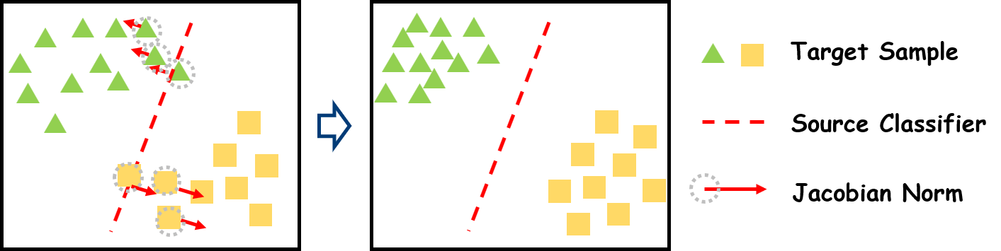
Figure 1: We propose a Jacobian norm regularizer, which effectively utilizes the neighbor information of the target sample to boost the performance of USFDA.

• We theoretically provide a new-brand target generalization bound based on the Total Variation distance [26] and model smoothness, which provides a novel insight for solving USFDA.

• We develop a simple yet general JN regularizer to boost the performance of USFDA, which can be easily incorporated into any existing USFDA methods as a plug-in unit with a few lines of code increased.

• We empirically find that JN regularizer can significantly improve the performance of the existing USFDA method, which achieves competitive results on multiple datasets.

The remainder of this paper is organized as follows. In Section II, we briefly overview unsupervised domain adaptation and unsupervised source-free domain adaptation. In Section III, we present the problem definition and derive a new-brand target generalization error bound. In Section IV, We develop the JN regularizer and the entire USFDA model to address USFDA. The experimental results and the post-hoc analysis are reported in Section V. In the end, we conclude the entire paper with future research directions in Section VI.

II Related Works

In this section, we present the most related researches on UDA/USFDA and highlight the differences between these methods and ours.

II-A Unsupervised Domain Adaptation

Recent practices on UDA usually attempt to minimize the domain discrepancy for knowledge transfer. Following this, multiple domain adaptation techniques have been developed, which can be summarized into the sample alignment [15, 16, 17] and feature alignment [18, 27, 19]. In particular, the sample alignment methods focus on mitigating the between-domain divergence such as the $\mathcal{A}$-distance [17], Maximum Mean Discrepancy (MMD) [16], or KL-divergence [15] through re-weighting the individual samples. In contrast, the feature alignment methods generate the domain-invariant feature through kernel matching [18], adversarial learning [19], transferrable contrastive learning [28], prototype matching [5], optimal transport [20] and image reconstruction [21], to reduce the distribution differences across domains, such as MMD [18], central moment discrepancy [29], Joint MMD [30], $\mathcal{A}$-distance [19] and maximum classifier discrepancy [31], Wasserstein distance [32], etc.

Compared with the UDA methods which require access to both source and target data, our work does NOT require the source data while learning to adapt. This is more suitable in real-world applications.

II-B Unsupervised Source-Free Domain Adaptation

Different from UDA, USFDA is a more practical scenario in which the source data is inaccessible at adaptation. Existing methods seek to implicitly align the target domain feature to the source domain by heuristically leveraging the information from the source model. The conventional USFDA methods include pseudo labelling (e.g., SHOT [33] and BAIT [34]), batch normalization (e.g., BN [35]) or data generation (e.g., MA [23]). Specifically, the pseudo labelling methods implicitly align representations from the target domains to the source model, the BN method minimizes the discrepancy between domains by BN statistics stored in the source model, and the image generation methods align the target domain to the annotated data generated by source model.

The existing USFDAs mainly focus on mitigating the between-domain divergence, which often neglect the neighbor information. Instead, the proposed JN regularization term focuses on optimizing the model smoothness to leverage the neighbor information from the target domain itself, which can be used as a plug-in unit to effectively boost performance of the existing USFDAs.

III Model Smoothness for Target Generalization Error Bound

The current theoretical works on domain adaptation are typically established on domain discrepancy, which encourages domain alignment in solving domain adaptation [14, 13]. However, in USFDA, due to the absence of source data, such an alignment is often difficult and insufficient. To boost the adaptation ability of USFDA, we now look back upon the origin of domain adaptation and attempt to induce a novel insights for addressing USFDA.

III-A Preliminaries

In this paper, we focus on the USFDA task. We use $\mathcal{X}\subset\mathbb{R}^{d}$ and $\mathcal{Y}\subset\mathbb{R}$ to denote the feature and the label space, respectively. We assume that the feature space $\mathcal{X}$ of source and target domain has a compact support. Thus, there exists a constant $D>0$, such that $\forall{\mathbf{u,v}\in\mathcal{X}},\|\mathbf{u-v}\|<D$. In particular, we are given $n$ labeled samples $\{x_{i}^{s},y_{i}^{s}\}_{i=1}^{n}$ from the source domain $\mathcal{D}_{s}$ with the distribution $\mathbb{P}$, where $x_{i}^{s}\in\mathcal{X}$ and $y_{i}^{s}\in\mathcal{Y}$. We also have $m$ unlabeled samples $\{x_{i}^{t}\}_{i=1}^{m}$ from $\mathcal{D}_{t}$ with the distribution $\mathbb{Q}$, where $x_{i}^{t}\in\mathcal{X}$. In the USFDA setting, $\mathbb{P}\neq\mathbb{Q}$ and the source data can be only accessed at the source model training procedure. In particular, we consider the K-way classification task. The goal of the USFDA is to learn a target function $f:\mathcal{X}\rightarrow\mathcal{Y}$ and predict the target label $\{y_{i}^{t}\}_{i=1}^{m}$, where $y_{i}^{t}\in\mathcal{Y}$, with only target data $\{x_{i}^{t}\}_{i=1}^{m}$ and the source function $f_{s}:\mathcal{X}\rightarrow\mathcal{Y}$ available in adaptation.

In addition, let $\mathcal{L}(f(\mathbf{x}),y)$ be the continuous and differentiable loss function. Inspired by a current theoretical study [36], we assume that $0\leq\mathcal{L}(f(\mathbf{x}),y)\leq M$ for constant $M$ without loss of generality. Moreover, we denote the $\mathcal{E}_{\mathbb{P}}\left(f\right)=\mathbb{E}_{\{x,y\}\sim\mathbb{P}}\mathcal{L}(f(x),y)$ as the expected risk of model $f$ over distribution $\mathbb{P}$. In order to find an alternative to mitigate the dilemma in USFDA. we also need the following definitions of Total Variation distance [26] and model smoothness:

Definition 1

Total Variation distance [26]: Given two distributions $\mathbb{P}$ and $\mathbb{Q}$. The Total Variation distance $\mathrm{TV}(\mathbb{P},\mathbb{Q})$ between distributions $\mathbb{P}$ and $\mathbb{Q}$ is defined as:

$$\mathrm{TV}(\mathbb{P},\mathbb{Q})=\frac{1}{2}\int_{\mathcal{X}}|d\mathbb{P}(\mathbf{x})-d\mathbb{Q}(\mathbf{x})|.$$ (1)

Definition 2

Model Smoothness : A model $f$ with parameter $\mathbf{w}$ is $r$-cover with $\epsilon$-smoothness on distribution $\mathbb{P}$, if

$$\mathbb{E}_{\mathbb{P}}\left[\sup_{\|\bm{\delta}\|_{\infty}\leq r}|f(\mathbf{x}+\bm{\delta})-f(\mathbf{x})|\right]\leq\epsilon.$$ (2)

where $\|\bm{\cdot}\|_{\infty}$ is the $l_{\infty}$-norm.

Remark: Since the source data is unavailable, the current theoretical works based on $\mathcal{H}$-divergence are often limited in the USFDA setting. Further, such a divergence is not consistent with the current domain alignment work [37] and let alone the existing USFDA works. In contrast, TV distance is more probabilistically interpretable and consistent with the objective of the existing USFDAs. In particular, pseudo-labeling attempts to minimize the KL-divergence between the one-hot encoding and the model output of the target domain[22], BN method also minimizes the KL-divergence between domains by utilizing batch normalization (BN) statistics stored in the source model [35]. Moreover, the image generation methods align the target domain to the annotated data by GAN, which is proven to be an approximation of TV distance [38]. Note that TV distance can be upper bounded in terms of KL-divergence as $TV(\mathbb{P},\mathbb{Q})\leq\sqrt{KL(\mathbb{P},\mathbb{Q})/{2\log e}}$ [39]. Thus, we conduct the TV distance to analyze the new target generalization error bound.

III-B Generalization Error Bound Via Model Smoothness

With the Total Variation distance in Definition 1 and model smoothness in Definition 2, we present our new-brand generalization error bound on target domain in Theorem 1.

Theorem 1

Given two distributions $\mathbb{P}$ and $\mathbb{Q}$, if a model $f$ is $2r$-cover with $\epsilon$ smoothness over distributions $\mathbb{P}$ and $\mathbb{Q}$, with probability at least $1-\theta$, we have:

$$\mathcal{E}_{\mathbb{Q}}\left(f\right)\leq\mathcal{E}_{\mathbb{P}}\left(f\right)+2 \epsilon+2M\mathrm{TV}(\mathbb{P},\mathbb{Q})$$ (3)

$$+M \sqrt{\frac{\left(2d\right)^{\frac{2\epsilon^{2}D}{r^{2}}+1}\log 2+2\log\left(\frac{1}{\theta}\right)}{m}}$$

$$+M \sqrt{\frac{\left(2d\right)^{\frac{2\epsilon^{2}D}{r^{2}}+1}\log 2+2\log\left(\frac{1}{\theta}\right)}{n}}$$

$$+M \sqrt{\frac{\log(1/\theta)}{2m}}.$$

The proof of Theorem 1 is given in the supplementary file. In contrast to the existing theoretical works, we utilize the TV-divergence $\mathrm{TV}(\mathbb{P},\mathbb{Q})$ to measure the domain discrepancy, since TV distance is more probabilistically interpretable and consistent with the objective of the existing USFDAs as mentioned. In particular, the model smoothness $\epsilon$ is firstly considered in adaptation, which provides a new perspective to address USFDA. To relieve the dilemma and boost the performance of the USFDA, we intuitively focus more on optimizing the new term $\epsilon$ to leverage the neighbor knowledge from the target domain.

IV Domain adaptation without Access to Source Data

In this section, following the idea of the theoretical result, we provide a novel learning framework to address USFDA. More precisely, for the model smoothness term, we present a JN regularizer on target domain as a plug-in unit to boost the existing USFDA, which implicitly forces the smoothness of model in the neighborhood of target sample. Subsequently, we adopt pseudo labelling strategy (i.e., SHOT [22]) as an attempt baseline to handle the domain discrepancy term, due to its simplicity.

Figure 2 shows a pipeline of our approach. Specifically, we first generate the source model by source data. During its development, we keep the classifier frozen and utilize the feature encoding module as initialization for target domain. The feature encoding module is then fine-tuned by our proposed framework. In the following, we elaborate each step of our model.

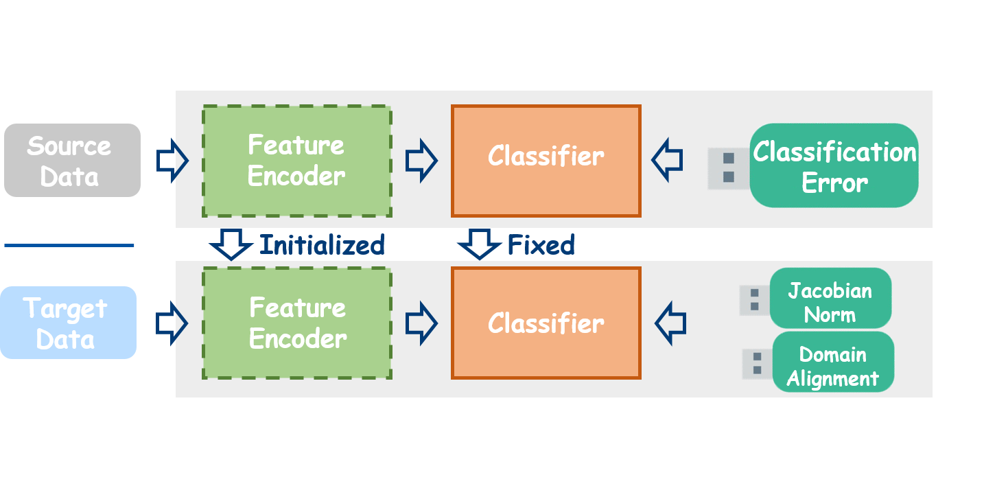
Figure 2: The pipeline of our approach: we freeze (solid line) the source classifier and fine-tune (dash line) the source encoding module. The source data is only available in source model training. The JN regularizer can be easily adopted as a plug-in unit to boost the adaptation performance.

IV-A Source Model Generation

To learn the source model for the subsequent target adaptation, referring to the baseline model [22], we adopt the cross-entropy loss based on label smoothing, as it increases the discriminability of the learned source model [40] . We have the following objective $\mathcal{L}_{s}$:

$$\mathcal{L}_{s}=-\mathbb{E}_{\left(x_{s},y_{s}\right)\in\mathcal{D}_{s}}\sum_{k=1}^{K}q_{k}^{ls}\log\left(\delta_{k}\left(f_{s}\left(x_{s}\right)\right)\right),$$ (4)

where $q_{k}^{ls}=(1-\alpha)q_{k}+\alpha/K$ is the smoothed label, $q_{k}$ is the one-of $K$ encoding and $\alpha$ is smoothing parameter empirically set to 0.1. $\delta_{k}\left(\cdot\right)$ denotes the $k$-th element in the soft-max output of a $K$-dimensional vector.

IV-B Target Model Fine-tuning

To make the fixed classifier/model works well in the target domain, we aim to obtain a fine-tuned encoder that could implicitly mitigate the domain discrepancy and optimize the model smoothness on target domain. Therefore, the objective function of our framework is formulated as follows:

$$\mathcal{L}_{t}=\mathcal{L}_{\mathcal{M}}+\mathcal{L}_{\mathcal{D}},$$ (5)

where $\mathcal{L}_{\mathcal{M}}$ denotes the model smoothness objective, and $\mathcal{L}_{\mathcal{D}}$ represents the domain alignment objective. Note that the current USFDAs focus on heuristically modelling the $\mathcal{L}_{\mathcal{D}}$, we aims to formulate $\mathcal{L}_{\mathcal{M}}$ , which can act as a plug-in unit to any existing USFDAs. These two terms are detailed in the following subsections:

IV-B1 Jacobian Norm for Model Smoothness

To formulate $\mathcal{L}_{\mathcal{M}}$, according to the Definition 2, we are motivated to control the smoothness/consistence in the neighborhood of the target sample. Along this line, we relax Eq. 2 for simplicity, and obtain the following objective:

$$\frac{1}{\sigma^{2}}\sum_{i=1}^{n_{t}}\mathbb{E}_{\zeta}\left(f\left(\mathbf{x}_{i}+\zeta\right)-f\left(\mathbf{x}_{i}\right)\right)^{2},$$ (6)

where $\zeta\sim N\left(0,\sigma^{2}\mathbf{I}\right)$. By first-order Taylor expansion, and let $\mathbf{J}(\mathbf{x})=\frac{\partial\mathbf{f}}{\partial\mathbf{x}}\in R^{K\times D}$, we have

$$f(\mathbf{x}+\zeta)=f(\mathbf{x})+\mathbf{J}(\mathbf{x})\zeta+\bm{o}(\zeta).$$ (7)

Omitting the high-order terms, Eq. 6 can be reformulated to the following JN regularizer ($\mathcal{L}_{\mathcal{J}}$):

$$\mathcal{L}_{\mathcal{J}} =\frac{1}{\sigma^{2}}\sum_{i=1}^{n_{t}}\mathbb{E}_{\zeta}\left(f\left(\mathbf{x}_{i}\right.\right.\left.+\zeta)-f\left(\mathbf{x}_{i}\right)\right)^{2}$$ (8)

$$=\frac{1}{\sigma^{2}}\sum_{i=1}^{n_{t}}\mathbb{E}_{\zeta}\left\|\mathbf{J}\left(\mathbf{x}_{i}\right)\zeta\right\|^{2}$$

$$=\sum_{i=1}^{n_{t}}\operatorname{tr}\left[\mathbf{J}\left(\mathbf{x}_{i}\right)^{T}\mathbf{J}\left(\mathbf{x}_{i}\right)\frac{1}{\sigma^{2}}\mathbb{E}_{\zeta}\left[\zeta\zeta^{T}\right]\right]$$

$$=\sum_{i=1}^{n_{t}}\operatorname{tr}\left[\mathbf{J}\left(\mathbf{x}_{i}\right)^{T}\mathbf{J}\left(\mathbf{x}_{i}\right)\frac{1}{\sigma^{2}}\sigma^{2}\mathbf{I}\right]$$

$$=\sum_{i=1}^{n_{t}}\left\|\mathbf{J}\left(\mathbf{x}_{i}\right)\right\|_{F}^{2}.$$

Consequently, we formulate $\mathcal{L}_{\mathcal{M}}$ to JN regularizer $\mathcal{L}_{\mathcal{J}}$ where $\lambda$ is the balancing hyper-parameters.

$$\mathcal{L}_{\mathcal{M}}=\lambda\mathcal{L}_{\mathcal{J}}=\lambda\sum_{i=1}^{n_{t}}\left\|\mathbf{J}\left(\mathbf{x}_{i}\right)\right\|_{F}^{2}.$$ (9)

IV-B2 Nearest Centroid classifier for Obtaining Pseudo Label

To alleviate the harmful effects caused by the inaccurate network outputs, we further apply pseudo-labeling for each unlabeled data to better supervise the target data encoding training. Inspired by the DeepCluster [41], we first attain the centroid for each class in the target domain as follows:

$$c_{k}^{(0)}=\frac{\sum_{x_{t}\in\mathcal{X}_{t}}\delta\left(\hat{f}_{t}^{(k)}(x)\right)\hat{g}_{t}(x)}{\sum_{x_{t}\in\mathcal{X}_{t}}\delta\left(\hat{f}_{t}^{(k)}(x)\right)},$$ (10)

where $\hat{f}_{t}$ denotes the previously learned target model and $\hat{g}_{t}(x)$ is the target encoder. Then, we obtain the pseudo labels via the nearest centroid classifier

$$\hat{y}_{t}=\arg\min_{k}D_{f}\left(\hat{g}_{t}\left(x_{t}\right),c_{k}^{(0)}\right),$$ (11)

where $D_{f}(\cdot,\cdot)$ measures the cosine distance. In the end, the target centroids is computed via the new pseudo labels:

$$c_{k}^{(1)}=\frac{\sum_{x_{t}\in\mathcal{X}_{t}}\mathbb{I}\left(\hat{y}_{t}=k\right)\hat{g}_{t}(x)}{\sum_{x_{t}\in\mathcal{X}_{t}}\mathbb{I}\left(\hat{y}_{t}=k\right)},$$ (12)

where $\mathbb{I}$ is the index function. The final pseudo label is obtained as followings:

$$\hat{y}_{t}=\arg\min_{k}D_{f}\left(\hat{g}_{t}\left(x_{t}\right),c_{k}^{(1)}\right),$$ (13)

IV-B3 Pseudo Labeling for Implicit Alignment

To formulate the $\mathcal{L}_{\mathcal{D}}$, referring to the baseline [22], we adopt both the information maximization loss $\mathcal{L}_{IM}$ and self-supervised pseudo labelling loss $\mathcal{L}_{SSL}$ toward implicit alignment. Their formulations are as follows, respectively:

$$\mathcal{L}_{IM}=-H\left(\frac{1}{K}\sum_{i}^{K}f\left(x_{i}\right)\right)+\frac{1}{K}\sum_{i}^{K}H\left(f\left(x_{i}\right)\right),$$ (14)

$$\mathcal{L}_{SSL}=-\mathbb{E}_{\left(x_{t}\right)\in\mathcal{D}_{t}}\sum_{k=1}^{K}\hat{q}_{k}\log\left(\delta_{k}\left(f\left(x_{t}\right)\right)\right),$$ (15)

where $H(\cdot)$ is the entropy function. $\hat{q}_{k}$ is the one-of-$K$ encoding of the target pseudo labels, which is generated by the nearest centroid classifier. For more details, please refer to [22]. In this way, we define $\mathcal{L}_{\mathcal{D}}$ as the composition of $\mathcal{L}_{IM}$ and $\mathcal{L}_{SSL}$:

$$\mathcal{L}_{\mathcal{D}}=\beta\mathcal{L}_{IM}+\gamma\mathcal{L}_{SSL},$$ (16)

where $\beta$ and $\gamma$ are the balancing hyper-parameters and we empirically set $\beta=1$ and $\gamma=1$ in our following experiments.

Last but not least importantly, we need to state that although our model is based on SHOT, for other USFDA methods, our framework can be easily applied by reformulating $\mathcal{L}_{\mathcal{D}}$. Therefore, the JN regularizer is flexible enough to be embedded into any other existing USFDAs.

TABLE I: Statistics of the benchmark datasets

Dataset	#Sample	#Class	#Domain
Office-31	4652	31	A, W, D
Office-Home	15500	65	Ar, Cl, Pr, Rw
VisDa-C	207000	12	Real, Synthesis

TABLE II: Classification accuracies (%) on small-sized Office-31 dataset (ResNet-50).

	DAN	DANN	CDAN	BSP	SO	MA	BAIT	BN	SHOT	JN(o)	Our Model
A$\rightarrow$D	78.6	79.7	92.9	93.0	80.1	92.7	92.0	89.0	92.1	88.8	95.9
A$\rightarrow$W	80.5	82.0	94.1	93.3	76.6	93.7	94.6	91.7	89.6	88.9	92.5
D$\rightarrow$A	63.6	68.3	71.0	74.6	60.5	75.3	74.6	78.5	74.1	72.7	75.4
D$\rightarrow$W	97.1	96.9	98.6	98.2	95.5	98.5	98.1	98.9	98.5	98.4	98.5
W$\rightarrow$A	62.8	67.4	69.3	72.6	63.4	77.8	73.9	76.6	73.3	73.4	77.4
W$\rightarrow$D	99.6	99.1	100	100	98.5	98.5	100	99.8	99.9	99.9	99.9
AVE	80.4	82.2	87.7	88.5	79.1	89.6	89.1	89.0	87.9	87.0	89.9
Due to the simplicity and the availability of source code, we only conduct SHOT as the baseline method. Specifically, our model is actually a JN regularized objective of SHOT, according to Eq.LABEL:eqo. The best accuracy is presented in bold and the second best is underlined, similarly hereinafter.

TABLE III: Classification accuracies (%) on medium-sized Office-Home dataset (ResNet-50).

	DAN	DANN	CDAN	BSP	SO	BAIT	SHOT	JN(o)	Our Model
Ar$\rightarrow$Cl	43.6	45.6	50.7	52.0	44.9	57.4	55.9	54.8	56.4
Ar$\rightarrow$Pr	57.0	59.3	70.6	68.6	66.5	77.5	77.8	76.6	78.6
Ar$\rightarrow$Re	67.9	70.1	76.0	76.1	74.3	82.4	80.7	82.0	82.0
Cl$\rightarrow$Ar	45.8	47.0	57.6	58.0	52.9	68.0	66.9	68.4	68.3
Cl$\rightarrow$Pr	56.5	58.5	70.0	70.3	62.8	78.2	77.3	73.9	80.1
Cl$\rightarrow$Re	60.4	60.9	70.0	70.2	65.1	78.1	77.1	76.3	79.4
Pr$\rightarrow$Ar	44.0	46.1	57.4	58.6	52.9	67.4	66.4	66.8	68.8
Pr$\rightarrow$Cl	43.6	43.7	50.9	50.3	41.5	55.5	53.6	54.6	55.1
Pr$\rightarrow$Re	67.7	68.5	77.3	77.6	73.4	81.7	81.5	81.3	82.2
Re$\rightarrow$Ar	63.1	63.2	70.9	72.2	65.4	76.3	72.1	74.2	75.3
Re$\rightarrow$Cl	51.5	51.8	56.7	59.3	45.4	57.1	57.2	58.4	58.8
Re$\rightarrow$Pr	74.3	76.8	81.6	81.9	77.9	84.3	83.0	83.3	84.6
AVE	56.3	57.6	65.8	66.3	60.2	70.8	71.5	70.6	74.5

TABLE IV: Classification accuracies (%) on large-sized VisDA-C dataset (ResNet-101).

	DAN	DANN	CDAN	BSP	SO	MA	BAIT	SHOT	JN(o)	Our Model
plane	87.1	81.9	85.2	92.4	76.1	94.8	93.7	94.6	94.6	95.1
bcycl	63.0	77.7	66.9	61.0	21.9	73.4	83.2	83.1	83.4	86.6
bus	76.5	82.8	83.0	81.0	51.1	68.8	84.5	73.3	80.3	78.3
car	42.0	44.3	50.8	57.5	70.3	74.8	65.0	54.3	56.8	62.1
horse	90.3	81.2	84.2	89.0	64.6	93.1	92.9	90.2	91.4	94.5
knife	42.9	29.5	74.9	80.6	16.0	95.4	95.4	67.1	92.5	96.4
mcycl	85.9	65.1	88.1	90.1	81.2	88.5	88.1	78.8	84.2	84.6
person	53.1	28.6	74.5	77.0	18.5	84.7	80.8	76.3	78.3	81.0
plant	49.7	51.9	83.4	84.2	69.3	89.1	90.0	89.6	87.6	90.2
sktbrd	36.3	54.6	76.0	77.9	28.4	84.7	89.0	87.2	88.9	89.5
train	85.8	82.8	81.9	82.1	84.3	83.6	84.0	87.3	87.3	84.7
truck	20.7	20.7	38.0	38.4	6.0	48.1	45.3	50.3	56.2	58.6
AVE	61.1	57.4	73.9	75.9	49.0	81.6	82.7	77.7	81.8	83.5

V Experiments

In this section, we present the experimental results on multiple domain adaptation benchmarks to demonstrate the effectiveness of our model.

V-A Benchmark Datasets

To evaluate the performance of our model, we conduct abundant experiments over the most widely-used benchmark datasets [4] with different sample size including Office-31 (small-size), Office-Home (medium size) and VisDA-C (large size). Table I lists the statistics of these datasets.
Office-31 ([42] is a small-size benchmark, which contains 4652 images with 31 categories in three visual domains Amazon(A), DSLR(D), Webcam(W).
Office-Home [43] is a medium-size benchmark, which contains 15588 images of 65 categories from 4 domains: Artistic images (Ar), Clipart images (Cl), Product images (Pr), and Real-world images (Rw).
VisDA-C ([44] is a large-scale benchmark, which contains 207000 images of 12 categories from synthesis and real domains. The source domain contains 152000 of synthetic images, while the target domain has 55000 real object images sampled from Microsoft COCO.

V-B Comparison Methods

To verify the effectiveness of the our work, we compare it respectively with several UDA and USFDA SOTAs. The UDA methods include Deep Adaptation Network (DAN) [45], Domain Adversarial Neural Networks (DANN) [19] Conditional Adversarial Networks (CDAN) [7] and Batch Spectral Penalization (BSP) [46]. The USFDA methods contain Source HypOthesis Transfer (SHOT) [22], Model Adaptation (MA) [23], BAIT [34] and Batch Normalization (BN) [35]. Moreover, source model only (SO) denotes using the entire source model for target label prediction. JN only (JN(o)) represents using JN regularizer only to fine-tune the feature encoder. It should be noted that SHOT is the baseline of our model by setting $\lambda=0$. To evaluate their performance, we follow the widely used accuracy as a measurement. The results of comparison methods are directly obtained from the published papers, since we follow the same setting.

V-C Implementation Details

V-C1 Network architecture

Following the current UDA/USFDA works [22, 30, 19], we employ the pre-trained ResNet-50 or ResNet-101 [47] models as the backbone module. Specifically, we replace the original FC layer with a bottleneck layer (256 units) and a task-specific FC classifier layer. After that, a BN layer is put inside the bottleneck layer. Moreover, a weight normalization layer is utilized in the last FC layer. More specifically, for each task, referring to the existing works [7, 48], we employ the pre-trained ResNet-50 (Office-31 and Office-Home) or ResNet-101 (VisDA-C) [47] models as the backbone module.

V-C2 Parameter Settings

To fine-tune the adaptive model, we adopt the mini-batch SGD with momentum 0.9 and set the batch size as 64. For Office-31 and Office-Home, we empirically set the learning rate as 0.01 and $\lambda=0.2$. Since VisDA-C can easily converge, we utilize a smaller learning rate 0.001 and a bigger $\lambda=0.8$. For learning in the target domain, we update the pseudo-labels epoch by epoch. The whole network is trained by the back propagation, while the newly added layers (e.g., task-specific FC classifier layer) are trained with learning rate 10 times of that of the pre-trained layers.

V-D Experimental Results

The experimental results of Office-31, Office-Home, and VisDA-C are reported in Tables II, III, and IV, respectively. From these results, we can make several observations as follows.

Firstly, by adding a simple JN regularization term, our model obtains the best mean accuracy on Office-31 and Office-Home, and the best per-class accuracy on Visda-Home. Compared with the USFDA SOTAs [23, 34, 35], we achieve the best/second-best results on 5 out of 6 individual tasks at Office-31 dataset and the best/second best on all 12 tasks at Office-Home dataset, respectively. For large-scale synthesis-to-real VisDA-C dataset, we achieve the best/second-best class accuracy among 9 out of 12 classes. These results obtained from a wide range of datasets with different sample sizes demonstrate that our model is capable of reducing the target risk while solving USFDA to great extent.

Secondly, compared to the conventional UDA works, we also achieve the competitive results even with no direct access to the source domain data. Specifically, our model achieves better gains with 1.4$\%$, 8.2$\%$ and 7.6$\%$ in performance than the UDA SOTAs on the Office-31, Office-Home and VisDA-C datasets, respectively. This implying the superior of our model even without source data.

Thirdly, compared to the baseline model (i.e, SHOT) which only achieves the second best results on two tasks at Office-31 dataset and one task at Office-Home, the designed JN regularizer provides gains on almost all tasks (e.g., $\sim$ 4% on A$\rightarrow$D and W$\rightarrow$A tasks). Moreover, the performance of our model only degrades in class ’train’ on VisDA-C, and the main reason may be that the background of this class is too complex.

TABLE V: Ablation Study: Components of Each Method

Dataset	SHOT	JN(o)	Our Model
Model Smoothness	✗	✓	✓
Implicit Alignment	✓	✗	✓

V-E Evaluation of Each Component

When solving the USFDA, our model involves two components: (1) Jacobian norm for model smoothness and (2)pseudo labeling for implicit alignment. To verify the performance of different components, we empirically select different components as shown in Table V. Specifically, SHOT only considers the implicit alignment, JN(o) only considers the model smoothness while our model contains both two terms.

As expected, compared to SHOT (i.e., $\mathcal{L}_{\mathcal{D}}$ only), the proposed JN regularizer provides a significant performance gain (i.e., 2% over Office-31, 3.7% over Office-Home and 5.8% over VisDA-C), which illustrates that implicit alignment is not sufficient to address USFDA and the proposed JN regularizer can effectively boost the performance of USFDA. Moreover,the results of JN alone (i.e., $\mathcal{L}_{\mathcal{J}}$ only) also achieves comparable results on USFDA with the accuracy of 87.0%, 70.6% and 81.8% on the Office-31, Office-Home and VisDA-C, respectively.

Those results demonstrate that both two components are important for improving the accuracy in USFDA tasks, which is consistent with the derived theoretical result in the Theorem 1. Moreover, the results further reveal that implicit alignment and model smoothness can benefit each other in solving USFDA.

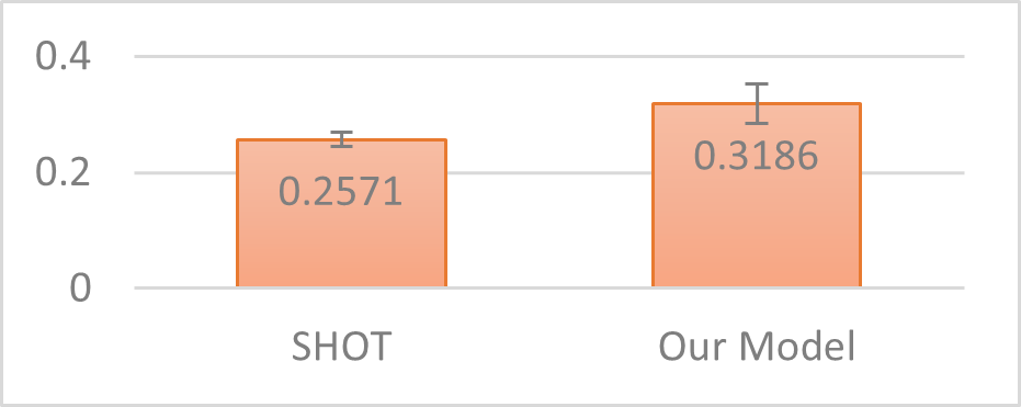
Figure 3: The time cost(s) of SHOT and our Model on the VisDA-C dataset. The error bar represents the standard deviation.

V-F Time Complexity

We validate the time complexity of the proposed JN regularizer through the empirical analysis. Specifically, we compare the time cost of our model with SHOT on the large-scale dataset, i.e., VisDA-C. The environment is Nvidia RTX 2080Ti with 11G memory. The results are given in Figure. 3. Specifically, for each batch, the proposed JN regularization term only introduces additional 0.06s cost on VisDA-C. As we can observe, despite its superiority in the performance gain, the time cost paid by the proposed JN regularization term is almost negligible.

VI Conclusion

In this paper, we develop a JN regularizer as a plug-in unit to boost the performance of USFDA. With a few lines of codes, the proposed JN regularizer can significantly improve the performance of the existing USFDAs. It is worth noting that the JN regularization term does NOT need access to the source model and thus can be applied on more challenging black-box USFDA, which will be further studied in our future work.

References

- [1] Y. Yao, Y. Zhang, X. Li, and Y. Ye, “Heterogeneous domain adaptation via soft transfer network,” in Proceedings of the 27th ACM international conference on multimedia, pp. 1578–1586, 2019.
- [2] W. M. Kouw and M. Loog, “A review of domain adaptation without target labels,” IEEE transactions on pattern analysis and machine intelligence, 2019.
- [3] W. Li and S. Chen, “Unsupervised domain adaptation with progressive adaptation of subspaces,” arXiv preprint arXiv:2009.00520, 2020.
- [4] S. Li, C. H. Liu, B. Xie, L. Su, Z. Ding, and G. Huang, “Joint adversarial domain adaptation,” in Proceedings of the 27th ACM International Conference on Multimedia, pp. 729–737, 2019.
- [5] Z. Wang, Y. Luo, Z. Huang, and M. Baktashmotlagh, “Prototype-matching graph network for heterogeneous domain adaptation,” in Proceedings of the 28th ACM International Conference on Multimedia, pp. 2104–2112, 2020.
- [6] M. Wang, W. Wang, B. Li, X. Zhang, L. Lan, H. Tan, T. Liang, W. Yu, and Z. Luo, “Interbn: Channel fusion for adversarial unsupervised domain adaptation,” in Proceedings of the 29th ACM International Conference on Multimedia, pp. 3691–3700, 2021.
- [7] M. Long, Z. Cao, J. Wang, and M. I. Jordan, “Conditional adversarial domain adaptation,” in Advances in Neural Information Processing Systems, pp. 1640–1650, 2018.
- [8] T. Jing, H. Xia, and Z. Ding, “Adaptively-accumulated knowledge transfer for partial domain adaptation,” in Proceedings of the 28th ACM International Conference on Multimedia, pp. 1606–1614, 2020.
- [9] Y. Cheng, F. Wei, J. Bao, D. Chen, F. Wen, and W. Zhang, “Dual path learning for domain adaptation of semantic segmentation,” in Proceedings of the IEEE/CVF International Conference on Computer Vision, pp. 9082–9091, 2021.
- [10] H. Guo, R. Pasunuru, and M. Bansal, “Multi-source domain adaptation for text classification via distancenet-bandits,” in Proceedings of the AAAI Conference on Artificial Intelligence, vol. 34, pp. 7830–7838, 2020.
- [11] S. Jiang, Z. Ding, and Y. Fu, “Deep low-rank sparse collective factorization for cross-domain recommendation,” in Proceedings of the 25th ACM international conference on Multimedia, pp. 163–171, 2017.
- [12] Y. Luo, Z. Huang, Z. Wang, Z. Zhang, and M. Baktashmotlagh, “Adversarial bipartite graph learning for video domain adaptation,” in Proceedings of the 28th ACM International Conference on Multimedia, pp. 19–27, 2020.
- [13] S. Ben-David, J. Blitzer, K. Crammer, F. Pereira, et al., “Analysis of representations for domain adaptation,” Advances in neural information processing systems, vol. 19, p. 137, 2007.
- [14] S. Ben-David, J. Blitzer, K. Crammer, A. Kulesza, F. Pereira, and J. W. Vaughan, “A theory of learning from different domains,” Machine learning, vol. 79, no. 1-2, pp. 151–175, 2010.
- [15] Y. Tsuboi, H. Kashima, S. Hido, S. Bickel, and M. Sugiyama, “Direct density ratio estimation for large-scale covariate shift adaptation,” Journal of Information Processing, vol. 17, pp. 138–155, 2009.
- [16] M. Sugiyama, T. Suzuki, S. Nakajima, H. Kashima, P. von Bünau, and M. Kawanabe, “Direct importance estimation for covariate shift adaptation,” Annals of the Institute of Statistical Mathematics, vol. 60, no. 4, pp. 699–746, 2008.
- [17] J. Huang, A. Gretton, K. Borgwardt, B. Schölkopf, and A. J. Smola, “Correcting sample selection bias by unlabeled data,” in Advances in neural information processing systems, pp. 601–608, 2007.
- [18] S. J. Pan, I. W. Tsang, J. T. Kwok, and Q. Yang, “Domain adaptation via transfer component analysis,” IEEE Transactions on Neural Networks, vol. 22, no. 2, pp. 199–210, 2010.
- [19] Y. Ganin and V. Lempitsky, “Unsupervised domain adaptation by backpropagation,” in International conference on machine learning, pp. 1180–1189, 2015.
- [20] W. Deng, Y. Cui, Z. Liu, G. Kuang, D. Hu, M. Pietikäinen, and L. Liu, “Informative class-conditioned feature alignment for unsupervised domain adaptation,” in Proceedings of the 29th ACM International Conference on Multimedia, pp. 1303–1312, 2021.
- [21] S. Sankaranarayanan, Y. Balaji, C. D. Castillo, and R. Chellappa, “Generate to adapt: Aligning domains using generative adversarial networks,” in 2018 IEEE/CVF Conference on Computer Vision and Pattern Recognition (CVPR), 2018.
- [22] J. Liang, D. Hu, and J. Feng, “Do we really need to access the source data? source hypothesis transfer for unsupervised domain adaptation,” in International Conference on Machine Learning, pp. 6028–6039, PMLR, 2020.
- [23] R. Li, Q. Jiao, W. Cao, H.-S. Wong, and S. Wu, “Model adaptation: Unsupervised domain adaptation without source data,” in Proceedings of the IEEE/CVF Conference on Computer Vision and Pattern Recognition, pp. 9641–9650, 2020.
- [24] M. Ye, J. Zhang, J. Ouyang, and D. Yuan, “Source data-free unsupervised domain adaptation for semantic segmentation,” in Proceedings of the 29th ACM International Conference on Multimedia, pp. 2233–2242, 2021.
- [25] R. Siry, L. Hémadou, L. Simon, and F. Jurie, “On the inductive biases of deep domain adaptation,” CoRR, vol. abs/2109.07920, 2021.
- [26] C. Villani, Optimal transport: old and new, vol. 338. Springer, 2009.
- [27] B. Fernando, A. Habrard, M. Sebban, and T. Tuytelaars, “Unsupervised visual domain adaptation using subspace alignment,” in Proceedings of the IEEE international conference on computer vision, pp. 2960–2967, 2013.
- [28] Y. Chen, Y. Pan, Y. Wang, T. Yao, X. Tian, and T. Mei, “Transferrable contrastive learning for visual domain adaptation,” in Proceedings of the 29th ACM International Conference on Multimedia, pp. 3399–3408, 2021.
- [29] W. Zellinger, T. Grubinger, E. Lughofer, T. Natschläger, and S. Saminger-Platz, “Central moment discrepancy (cmd) for domain-invariant representation learning,” arXiv preprint arXiv:1702.08811, 2017.
- [30] M. Long, H. Zhu, J. Wang, and M. I. Jordan, “Deep transfer learning with joint adaptation networks,” in International conference on machine learning, pp. 2208–2217, 2017.
- [31] K. Saito, K. Watanabe, Y. Ushiku, and T. Harada, “Maximum classifier discrepancy for unsupervised domain adaptation,” in Proceedings of the IEEE Conference on Computer Vision and Pattern Recognition, pp. 3723–3732, 2018.
- [32] N. Courty, R. Flamary, and D. Tuia, “Domain adaptation with regularized optimal transport,” in Joint European Conference on Machine Learning and Knowledge Discovery in Databases, pp. 274–289, Springer, 2014.
- [33] K. Liang, J. Y. Zhang, O. Koyejo, and B. Li, “Does adversarial transferability indicate knowledge transferability?,” arXiv preprint arXiv:2006.14512, 2020.
- [34] S. Yanga, Y. Wanga, J. van de Weijera, L. Herranza, and S. Juic, “Casting a bait for offline and online source-free domain adaptation,” arXiv preprint arXiv:2010.12427, 2021.
- [35] M. Ishii and M. Sugiyama, “Source-free domain adaptation via distributional alignment by matching batch normalization statistics,” arXiv preprint arXiv:2101.10842, 2021.
- [36] M. Yi, L. Hou, J. Sun, L. Shang, X. Jiang, Q. Liu, and Z.-M. Ma, “Improved ood generalization via adversarial training and pre-training,” arXiv preprint arXiv:2105.11144, 2021.
- [37] C. Shui, Q. Chen, J. Wen, F. Zhou, C. Gagné, and B. Wang, “Beyond h-divergence: Domain adaptation theory with jensen-shannon divergence,” arXiv preprint arXiv:2007.15567, 2020.
- [38] Z. Pan, W. Yu, B. Wang, H. Xie, V. S. Sheng, J. Lei, and S. Kwong, “Loss functions of generative adversarial networks (gans): opportunities and challenges,” IEEE Transactions on Emerging Topics in Computational Intelligence, vol. 4, no. 4, pp. 500–522, 2020.
- [39] F. Nielsen and K. Sun, “Guaranteed deterministic bounds on the total variation distance between univariate mixtures,” in 2018 IEEE 28th International Workshop on Machine Learning for Signal Processing (MLSP), pp. 1–6, IEEE, 2018.
- [40] R. Müller, S. Kornblith, and G. Hinton, “When does label smoothing help?,” Advances in neural information processing systems, 2019.
- [41] M. Caron, P. Bojanowski, A. Joulin, and M. Douze, “Deep clustering for unsupervised learning of visual features,” in Proceedings of the European conference on computer vision (ECCV), pp. 132–149, 2018.
- [42] K. Saenko, B. Kulis, M. Fritz, and T. Darrell, “Adapting visual category models to new domains,” in European conference on computer vision, pp. 213–226, Springer, 2010.
- [43] H. Venkateswara, J. Eusebio, S. Chakraborty, and S. Panchanathan, “Deep hashing network for unsupervised domain adaptation,” in Proceedings of the IEEE Conference on Computer Vision and Pattern Recognition, pp. 5018–5027, 2017.
- [44] X. Peng, Z. Huang, X. Sun, and K. Saenko, “Domain agnostic learning with disentangled representations,” in International Conference on Machine Learning, pp. 5102–5112, PMLR, 2019.
- [45] M. Long, Y. Cao, J. Wang, and M. Jordan, “Learning transferable features with deep adaptation networks,” in International conference on machine learning, pp. 97–105, 2015.
- [46] X. Chen, S. Wang, M. Long, and J. Wang, “Transferability vs. discriminability: Batch spectral penalization for adversarial domain adaptation,” in International conference on machine learning, pp. 1081–1090, PMLR, 2019.
- [47] K. He, X. Zhang, S. Ren, and J. Sun, “Deep residual learning for image recognition,” in Proceedings of the IEEE conference on computer vision and pattern recognition, pp. 770–778, 2016.
- [48] C. Chen, W. Xie, W. Huang, Y. Rong, X. Ding, Y. Huang, T. Xu, and J. Huang, “Progressive feature alignment for unsupervised domain adaptation,” in Proceedings of the IEEE/CVF Conference on Computer Vision and Pattern Recognition, pp. 627–636, 2019.