Version:

Categorical Distributions of Maximum Entropy
under Marginal Constraints

Orestis Loukas,  Ho Ryun Chung

Institute for Medical Bioinformatics and Biostatistics
Philipps-Universität Marburg
Hans-Meerwein-Straße 6, 35032 Germany

Abstract

The estimation of categorical distributions under marginal constraints summarizing some sample from a population in the most-generalizable way is key for many machine-learning and data-driven approaches. We provide a parameter-agnostic theoretical framework that enables this task ensuring (i) that a categorical distribution of Maximum Entropy under marginal constraints always exists and (ii) that it is unique. The procedure of iterative proportional fitting (ipf) naturally estimates that distribution from any consistent set of marginal constraints directly in the space of probabilities, thus deductively identifying a least-biased characterization of the population. The theoretical framework together with ipf leads to a holistic workflow that enables modeling any class of categorical distributions solely using the phenomenological information provided.

1 Introduction

Most data-scientific problems explicitly or implicitly involve the estimation of a multivariate probability distribution of features from samples of a population. Once determined, such probability distribution allows for computing all interesting measures that describe the population [1]. For example, classification relies on the conditional probability of a target-feature given the characteristics of predictor-features, which can be readily computed from the joint probability distribution of target- and predictor-features. Another common task in data science is the determination of meaningful pair-wise or higher-order associations to understand the dependency structure among features. For example, it is of interest in epidemiology and related fields to determine the contributions of various “risk factors” or combinations thereof to the probability of becoming diseased. The presence of associations between risk-factors and a disease can be inferred from generalized odds-ratios, which, in turn, can be readily computed from the joint probability distribution of risk-factors plus disease characteristics.

Current approaches in statistical learning usually start with a parametric model for the joint probability distribution of features that captures the perceived or assumed associations between those features. Parametric modeling has offered convenient ways to approximate and efficiently implement tasks such as classification and feature extraction, thus becoming state of the art. In the big-data era, as evidence from larger datasets becomes stronger, more detailed structures of feature associations become amenable to analysis leading to the design of more complex, less intuitively comprehensible models. This emphasizes two main problems of parametric modeling pertaining to the restriction to probability distributions of the exponential family and the requirement to only choose parameterizations reflecting independent information obtained about the modeled features.

In this work, we adopt a fully data-driven parameter-agnostic approach to estimate the joint probability distribution of categorical features by casting modeling into an optimization problem in linear algebra. The guiding principle of this approach is the maximization of the entropy functional under phenomenological constraints imposed by the provided dataset. Starting from the information derived from samples of a population this alternative formulation of modeling deductively leads to the characterization of the population in the least-biased, most-generalizable way. At an operational level, we employ the old method of iterative proportional fitting [2, 3, 4] to estimate probability distributions after incorporating the desired pieces of information from the data by maximizing the entropy functional. Naturally formulated in terms of the probabilities of possible configurations of features, ipf automatically incorporates any relevant information that pertains to pair-wise and, in fact, higher-order associations without modification of the algorithm, augmenting the domain of probability distributions beyond the exponential family. We showcase the combined power of the principle of Maximum Entropy (maxent) and ipf by uncovering feature associations in a public dataset from emergency departments in the usa beyond the usually considered pair-wise level.

In summary, working in the space of probabilities not only preserves interpretability at any modeling stage, but considerably enhances the class of distributions from which all desired metrics can be then computed. Encoding phenomenological information as a linear system to apply the maxent principle clearly forms a deductive way to select an optimal solution. At the same time, the flexibility of ipf helps efficiently tackle the wealth of heterogeneous data encountered in realistic settings.

2 Problem formulation

In most data-driven studies, the goal is to estimate a sufficiently generalizable joint probability distribution of the investigated features that should characterize a population using information derived from samples of this population. In our problem formulation and its solution, we concentrate on categorical features making no restriction on the amount while systematizing the form of information that enters the estimation procedure.

Concretely, assume that we are given $L$ categorical features labeled by index $i\in\{1,\ldots,L\}$. Each feature $i$ can take an a priori different number $q_{i}\in\mathbb{N}$ of states (evidently $q_{i}\geq 2$) described by state variable $\alpha_{i}\in\{1,...,q_{i}\}$. A particular realization $(\alpha_{1},\ldots,\alpha_{L})$ specifying all state variables is called a microstate of the system under investigation. To formalize our notation we introduce the space of microstates

$$\mathcal{A}=\left\{(\alpha_{1},\ldots,\alpha_{L})~{}|~{}\alpha_{1}\in\{1,...,q_{1}\},\ldots,\alpha_{L}\in\{1,...,q_{L}\}\right\}$$ (1)

of dimension ${\left|\mathcal{A}\right|}=q_{1}\cdots q_{L}$. A probability distribution assigns to each microstate $\vec{\alpha}\in\mathcal{A}$ some real value $\mathfrak{p}(\vec{\alpha})\in[0,1]$ such that the sum of $\mathfrak{p}(\vec{\alpha})$ over $\mathcal{A}$ remains always normalized to unity. When clear from context, we shall use $\alpha$ as a vector index to enumerate microstates. In that way, any distribution $\mathfrak{p}$ can be regarded as an $\left|\mathcal{A}\right|$-dimensional column vector with entries between 0 and 1, motivating the more general definition of the space of probabilities

$$\mathcal{P}=\bigg{\{}\mathfrak{p}\in\mathbb{R}^{\left|\mathcal{A}\right|}~{}\big{|}~{}\mathfrak{p}_{\alpha}\in\mathbb{R}^{+}_{0}~{}\text{ for }~{}\alpha=1,\ldots,{\left|\mathcal{A}\right|}\quad\text{and}\quad\sum_{\alpha=1}^{\left|\mathcal{A}\right|}\mathfrak{p}_{\alpha}=1\bigg{\}}~{}.$$ (2)

Notice that $\mathfrak{p}\in\mathcal{P}$ implies $0\leq\mathfrak{p}_{\alpha}\leq 1$ for all $\alpha=1,\ldots,{\left|\mathcal{A}\right|}$. In the following, any model is automatically understood to be described by a distribution on the probability simplex $\mathcal{P}$ over the declared mictostates Eq. (1).

Usually, we are given a data matrix $\mathbf{X}\in\mathcal{M}_{N\times L}(\mathbb{N})$ with the records from a sample of size $N$ in the rows and the features along the columns. Each row of $\mathbf{X}$ is a microstate vector $\mathbf{X}_{j,\mathbf{\cdot}}\in\mathcal{A}$, whose $i$-th entry gives the state $\alpha_{i}$ in which the $i$-th feature was found in the $j$-th record. Conveniently, the data matrix $\mathbf{X}$ can be summarized by an empirical distribution $\mathfrak{f}\in\mathcal{P}$ of relative frequencies over the microstates,

$$\mathfrak{f}(\alpha_{1},\ldots,\alpha_{L})=\frac{1}{N}\sum_{j=1}^{N}\delta(\alpha_{1},X_{j,1})\cdots\delta(\alpha_{L},X_{j,L})~{},$$ (3)

where $\delta(\alpha,\beta)$ denotes the Kronecker delta when dealing with categorical variables $\alpha,\beta$. As we are interested in the associations within sets of features with various cardinalities $\ell\leq L$, the information that enters the estimation of a model distribution $\mathfrak{p}$ shall be in form of marginal relative frequencies computed from the empirical distribution $\mathfrak{f}$. In a subset consisting of $\ell$ features labeled by $\{i_{1},\ldots,i_{\ell}\}$ where $1\leq i_{1}<\ldots<i_{\ell}\leq L$ with realizations $a\equiv(\alpha_{i_{1}},\ldots,\alpha_{i_{\ell}})$, a marginal relative frequency

$$\widehat{m}_{a}\equiv\mathfrak{f}_{i_{1},...,i_{\ell}}(\alpha_{i_{1}},\ldots,\alpha_{i_{\ell}})=\sum_{\alpha_{i_{\ell+1}}=1}^{q_{i_{\ell+1}}}\cdots\sum_{\alpha_{i_{L}}=1}^{q_{i_{L}}}\mathfrak{f}(\alpha_{1},\ldots,\alpha_{L})$$ (4)

is computed by summing the empirical distribution over the remaining $L-\ell$ directions in $\mathcal{A}$ that do not belong to cluster $\{i_{1},\dots,i_{\ell}\}$. Corresponding marginal probabilities $m_{a}$ can be calculated from any model joint distribution $\mathfrak{p}\in\mathcal{P}$ as

$$m_{a}\equiv\mathfrak{p}_{i_{1},...,i_{\ell}}(\alpha_{i_{1}},\ldots,\alpha_{i_{\ell}})=\sum_{\alpha_{i_{\ell+1}}=1}^{q_{i_{\ell+1}}}\cdots\sum_{\alpha_{i_{L}}=1}^{q_{i_{L}}}\mathfrak{p}(\alpha_{1},\ldots,\alpha_{L})~{}.$$ (5)

The marginal distributions $\mathfrak{p}_{i_{1},...,i_{\ell}}$ inherit the properties of non-negativity and normalization from $\mathcal{P}$. Similarly to the joint distribution, any marginal distribution $\mathfrak{p}_{i_{1},...,i_{\ell}}$ can be locally represented by a column vector of dimension $q_{i_{1}}\cdots q_{i_{\ell}}$ such that all specified marginal probabilities of $\mathfrak{p}$ can be conveniently encoded as a linear operation

$$m_{a}=\sum_{\alpha=1}^{\left|\mathcal{A}\right|}C_{a\alpha}\,\mathfrak{p}_{\alpha}~{}.$$ (6)

The columns of the binary architecture matrix $\mathbf{C}\in\mathcal{M}_{D\times\left|\mathcal{A}\right|}(\mathbb{N})$ correspond to the probability directions in $\mathcal{P}$ indexed by Greek $\alpha$ whereas its rows enumerate using Latin index $a$ the $D$ marginal probabilities we wish to incorporate into our model. Since modeling from empirical data is usually concerned with under-constrained problems where $\text{rank}\,\mathbf{C}<{\left|\mathcal{A}\right|}$, the matrix $\mathbf{C}$ is expected to be singular in most applications. In other words, marginal probabilities $m_{a}$ and design architecture matrix $\mathbf{C}$ do not unambiguously determine the joint distribution $\mathfrak{p}$.

In practical applications, only limited information about marginal relative frequencies Eq. (4) in various (possibly intersecting) subsets of features might be accessible, leaving other marginal sums unspecified. Henceforth, we refer to the set of all marginal relative frequencies $\{\widehat{m}_{a}\}_{a=1,\ldots,D}$ that are accessible and provided in the problem statement as the summary statistics of empirical distribution $\mathfrak{f}$. Naturally, adhering to the empirical summary statistics induces an equivalence class on the simplex $\mathcal{P}$,

$$[\mathfrak{f}]=\left\{\mathfrak{p}\in\mathcal{P}~{}|~{}\sum_{\alpha=1}^{\left|\mathcal{A}\right|}C_{a\alpha}\,(\mathfrak{p}_{\alpha}-\mathfrak{f}_{\alpha})=0\quad\forall a=1,...,D\right\}~{}.$$ (7)

By definition, any distribution $\mathfrak{p}\in\mathcal{P}$ belonging to the equivalence class shares the same summary statistics with $\mathfrak{f}$. In the two extreme cases where either the set of marginal probabilities is empty or saturated, it is $[\mathfrak{f}]=\mathcal{P}$ and $[\mathfrak{f}]=\{\mathfrak{f}\}$, respectively. Any other summary statistics of $\mathfrak{f}$ constitutes the realm of non-trivial model building.

The information contained in the provided set of marginal relative frequencies from empirical distribution $\mathfrak{f}$ necessarily constrains the space of admissible $\mathfrak{p}\in\mathcal{P}$ to the equivalence class $[\mathfrak{f}]$ inducing a system of coupled linear equations

$$m_{a}\equiv\sum_{\alpha=1}^{\left|\mathcal{A}\right|}C_{a\alpha}\,\mathfrak{p}_{\alpha}\overset{!}{=}\sum_{\alpha=1}^{\left|\mathcal{A}\right|}C_{a\alpha}\,\mathfrak{f}_{\alpha}\equiv\widehat{m}_{a}\quad\forall\,a=1,...,D~{}.$$ (8)

At finite $N$, the linear problem corresponds to finding all member distributions of the equivalence class $[\mathfrak{f}]$. Multiplying Eq. (8) by $N$ gives a so-called Diophantine system of coupled linear equations. More generally when $N\rightarrow\infty$, it becomes a system of linear equations in $\left|\mathcal{A}\right|$ variables $\mathfrak{p}_{\alpha}\in\mathbb{R}_{0}^{+}$ for each tuple $(\alpha_{i_{1}},...,\alpha_{i_{\ell}})$ in each subset $\{i_{1},\ldots,i_{\ell}\}$. Being an equivalence class in $\mathcal{P}$ the solution set to linear system Eq. (8) forms a non-empty convex subset of $\mathcal{P}$, whenever the summary statistics from some empirical distribution $\mathfrak{f}$ are provided, as it includes at least $\mathfrak{f}$ itself. The binary architecture matrix $\mathbf{C}$ introduced in Eq. (6) plays the role of the coefficient matrix, while the vector of marginal relative frequencies with components $\widehat{m}_{a}$ acts as the inhomogeneous term. The specification of marginal distribution $\mathfrak{f}_{i_{1},\ldots,i_{\ell}}$ in Eq. (4) in a feature set of cardinality $\ell$ automatically implies all lower marginal distributions $\mathfrak{f}_{i_{1},\ldots,i_{\nu}}$ with $\nu<\ell$ ($\nu=0$ being the normalization condition itself). This means that the system of linear constraints described by $\mathbf{C}$ is generically redundant, whenever the summary statistics of $\mathfrak{f}$ include marginal distributions on intersecting subsets of features.

Special care needs to be taken whenever any empirical marginal relative frequency $\widehat{m}_{a}$ is exactly zero. Due to the constraint of non-negativity on the simplex of Eq. (2), $\widehat{m}_{a}=0$ automatically sets all probabilities $\mathfrak{p}_{\alpha}$ contributing to $m_{a}\overset{!}{=}\widehat{m}_{a}$ via Eq. (6) to zero:

$$\exists\,a\in[1,D]:~{}~{}\widehat{m}_{a}=0\quad\Rightarrow\quad\mathfrak{p}_{\alpha}=0\quad\forall\,\alpha\in\{1,\ldots,{\left|\mathcal{A}\right|}\}~{}\text{ with }~{}C_{a\alpha}=1~{}.$$ (9)

We encounter [5] two types of $a$’s, i.e. realizations $(\alpha_{i_{1}},\ldots,\alpha_{i_{\ell}})$ in a feature subset $\{i_{1},\ldots,i_{\ell}\}$, with a marginal relative frequency $\widehat{m}_{a}=0$. One type, referred to as sampling zero is due to insufficient sampling of microstates $\alpha$ with a relatively small probability participating in the $a$-th marginal sum Eq. (4). Thus in principle, any sampling zero is expected to disappear by sufficiently increasing the sample size or via regularization. The other type, which is referred to as structural zero, is logically known to have zero value, because it corresponds to certain feature realizations that are impossible, e.g. being biologically male and pregnant. In contrast to sampling zeros, a structural zero encodes important deterministic relationships between features and their realizations.

As a deterministic constraint, the presence of structural zero(s) $\widehat{m}_{a}=0$ modifies the architecture of linear system Eq. (8). In order to describe the probabilistic constraints applied to the subset $\mathcal{A}^{\prime}\subseteq\mathcal{A}$ which only includes those microstates that are not associated with any structural zero, we first define a reduced coefficient matrix $\mathbf{C}^{\prime}$ with all rows corresponding to structural zeros and columns corresponding to the microstates with zero probability removed. From the rank-nullity theorem we know then that the degrees of freedom in $\mathcal{A}^{\prime}$ which remain unconstrained by the summary statistics are given by

$$\dim\ker\mathbf{C}^{\prime}=|\mathcal{A}^{\prime}|-\text{rank}\,\mathbf{C}^{\prime}~{},$$ (10)

where the rank of the reduced coefficient matrix defines the dimension of the linear problem, $d\equiv\text{rank}\,\mathbf{C}^{\prime}$. As long as the reduced coefficient matrix $\mathbf{C}^{\prime}$ implies $d<|\mathcal{A}^{\prime}|$, there exists a non-trivial equivalence class $[\mathfrak{f}]$ given the summary statistics, so that we anticipate non-trivial model estimation.

3 The principle of maximum entropy

In the previous section, we have outlined how information about the joint probability distribution of a population in form of summary statistics from its samples enters the estimation procedure. This yields the linear system in Eq. (8) which relates the marginal relative frequencies $\widehat{m}_{a}$ to some model $\mathfrak{p}\in\mathcal{P}$ via the binary architecture matrix $\mathbf{C}$. The solutions of Eq. (8) span the equivalence class $[\mathfrak{f}]$ of the empirical joint distribution $\mathfrak{f}$. Now, we need a mechanism to select one of the distributions $\hat{\mathfrak{p}}\in[\mathfrak{f}]$ as a “good” model for the data-generating process. In more mathematical terms, we need to find a functional of distributions over the equivalence class $\mathcal{[}\mathfrak{f}]$ whose extremization shall yield the desired model distribution $\hat{\mathfrak{p}}$.

Lacking any information about the joint distribution of categorical features other than the number $L$ of categorical features and their different number $q_{i}$ of states, all we know at this point is the number of microstates $\left|\mathcal{A}\right|$. The uniform distribution $\mathfrak{u}_{\alpha}=\left|\mathcal{A}\right|^{-1}$ is unique in that it encodes only this information and nothing more. Only the uniform distribution guarantees that any permutation in the order of microstates yields the same probability assignment. Any non-uniform probability distribution signifies the presence of additional information that distinguishes between microstates. Next, we are given the hint that we will receive a sample with $N$ records. This information does not give ground to any change in the uniform probability assignment yet. However, we could reason about the probability to receive a sample of size $N$, i.e. a data matrix $\mathbf{X}\in\mathcal{M}_{N\times L}(\mathbb{N})$ summarized by the relative frequency distribution $\mathfrak{f}\in\mathcal{P}$ of microstates. As discussed in A, the probability distribution to receive any such sample from a finite population follows a multivariate hypergeometric or approximately a multinomial distribution $\text{mult}(N\mathfrak{f};\mathfrak{u})$.

A large-$N$ expansion of the multinomial probability distribution yields

$$\text{mult}(N\mathfrak{f};\mathfrak{u})=\frac{N!}{\prod_{\alpha}(N\mathfrak{f}_{\alpha})!}\prod_{\alpha=1}^{\left|\mathcal{A}\right|}(\mathfrak{u}_{\alpha})^{N\mathfrak{f}_{\alpha}}=\exp\left\{NH[\mathfrak{f}]-N\log{\left|\mathcal{A}\right|}-\frac{\left|\mathcal{A}\right|-1}{2}\log N+\mathcal{O}\left(1\right)\right\}~{}.$$ (11)

The sample-dependent leading term corresponds to Shannon’s differential entropy

$$H[\mathfrak{f}]=-\sum_{\alpha=1}^{\left|\mathcal{A}\right|}\mathfrak{f}_{\alpha}\log\mathfrak{f}_{\alpha}~{},$$ (12)

which is a measure of uncertainty about the underlying process that generates data. Essentially, the entropy functional measures the opposite of information-theoretic distance of the uniform distribution $\mathfrak{u}$ from $\mathfrak{f}$,

$$H[\mathfrak{f}]=-D_{\textsc{kl}}(\mathfrak{f}\;\|\;\mathfrak{u})+\log\left|\mathcal{A}\right|~{},$$ (13)

where the Kullback–Leibler (kl) divergence or entropy of $\mathfrak{f}$ relative to $\mathfrak{u}$,

$$D_{\textsc{kl}}(\mathfrak{f}\;\|\;\mathfrak{u})=\sum_{\alpha=1}^{\left|\mathcal{A}\right|}\mathfrak{f}_{\alpha}\log\frac{\mathfrak{f}_{\alpha}}{\mathfrak{u}_{\alpha}}~{},$$ (14)

represents a conventional notion of distance between two probability distributions in the world of information geometry [6, 7, 8]. For any pair of distributions it is non-negative definite on account of Jensen’s inequality attaining a global minimum iff the two distributions coincide. Thus, with information only about the microstate space $\mathcal{A}$ and the sample size $N$ the most likely sample is the one whose empirical distribution $\mathfrak{f}$ maximizes Shannon’s entropy $H[\mathfrak{f}]$ at the global minimum of the associated kl divergence. Incidentally, the entropy functional also governs the large-$N$ expansion of the multinomial coefficient

$$W[N\mathfrak{f}]=\frac{N!}{\prod_{\alpha=1}^{{\left|\mathcal{A}\right|}}(N\mathfrak{f}_{\alpha})!}=\exp\left\{NH[\mathfrak{f}]-\frac{\left|\mathcal{A}\right|-1}{2}\log N+\mathcal{O}\left(1\right)\right\}~{},$$ (15)

which combinatorially describes all possible ways to assign $N$ indistinguishable entities to ${\left|\mathcal{A}\right|}$ attributes reproducing the observed multiplicities $N\mathfrak{f}$.

Eventually, we are given a sample of size $N$ with data matrix $\mathbf{X}\in\mathcal{M}_{N\times L}(\mathbb{N})$ summarized by the empirical distribution $\mathfrak{f}$ of microstates. As before, we extract information from $\mathfrak{f}$ in the form of marginal probabilities $\widehat{m}$ to set up the system of coupled linear equations in Eq. (8), constraining the space of viable distributions $\mathfrak{p}$ to the equivalence class $[\mathfrak{f}]$. The probability $p\,(\mathfrak{p}\;|\;[\mathfrak{f}])$ to obtain a distribution $\mathfrak{p}\in[\mathfrak{f}]$ is accordingly determined at large $N$ by

$$p\,(\mathfrak{p}\;|\;[\mathfrak{f}])=\left[\sum_{\mathfrak{p}^{\prime}\in[\mathfrak{f}]}\exp\left(NH[\mathfrak{p}^{\prime}]\right)\right]^{-1}\exp\left(NH[\mathfrak{p}]\right)~{},$$ (16)

on account of Eq. (11) and Eq. (15). Obviously, the probability $p\,(\mathfrak{p}\;|\;[\mathfrak{f}])$ is maximal whenever the entropy $H[\mathfrak{p}]$ is maximized. The principle of maximum likelihood (mle) dictates how to choose among the solutions $\mathfrak{p}\in[\mathfrak{f}]$ of the linear system a distribution

$$\hat{\mathfrak{p}}=\max_{\mathfrak{p}\in[\mathfrak{f}]}p\,(\mathfrak{p}\;|\;[\mathfrak{f}])$$ (17)

that maximizes Eq. (16). Hence, the most likely distribution $\hat{\mathfrak{p}}$ in the equivalence class $[\mathfrak{f}]$ is the one of maximum entropy. Any other distribution in $[\mathfrak{f}]$ appears at sufficiently large $N$ exponentially suppressed. This shows that mle coincides at large $N$ and the latest asymptotically with the principle of maximum entropy (maxent; [9]), which is also known as the principle of minimum discrimination information [10] in the statistics field.

The power of the maxent principle as a deductive mechanism to unambiguously choose an optimal solution $\hat{\mathfrak{p}}$ in $[\mathfrak{f}]$ is summarized by

Theorem 1.

Among all distributions $\mathfrak{p}$ in the equivalence class $[\mathfrak{f}]$ induced by marginal probabilities $m\overset{!}{=}\widehat{m}$ there always exists a unique probability distribution $\hat{\mathfrak{p}}$ having the maximum entropy in the given equivalence class, $\hat{\mathfrak{p}}=\max\limits_{\mathfrak{p}\in[\mathfrak{f}]}H[\mathfrak{p}]$.

This theorem, alongside further properties of the maxent solution are constructively proven in detail in B. Alternatively to the constructive proof of existence outlined in Appendix, Theorem 1 holds given that $[\mathfrak{f}]$ is a closed convex subset of $\mathcal{P}$. $\mathcal{P}$ is compact, while Shannon’s entropy is a continuous concave function over the simplex. Hence, $[\mathfrak{f}]$ is compact and Shannon’s entropy necessarily attains a maximum there. Strict concavity of $H$ ensures the uniqueness. In addition to the reasoning presented in this paper, one can axiomatically arrive [11, 12, 13] at the maxent principle as the unique mechanism to perform deduction from a provided dataset in a most minimalistic, least-biased way.

4 Iterative proportional fitting

As argued in Section 3, the maxent principle selects a “good” model distribution $\hat{\mathfrak{p}}$ from the solutions in the equivalence class $[\mathfrak{f}]$ induced by Eq. (8). Theorem 1 guarantees that $\hat{\mathfrak{p}}$ exists and is unique giving rise to a deductive mechanism to estimate a model distribution from information in the form of marginal relative frequencies $\widehat{m}$. In this section, we present the algorithmic procedure of iterative proportional fitting (ipf) directly applied to the estimation of a model joint distribution $\hat{\mathfrak{p}}$ for categorical features. This flexible algorithm can estimate model distributions that incorporate any order of associations between features, i.e. marginal constraints in subsets of different cardinalities, without any formal modification. The history of ipf is long dating back as early as 1937 [2]. Its breakthrough for estimation of missing cells in contingency tables happened mainly due to [5]. In information theory, classical papers such as [14, 15] proved its convergence while exploring [16, 17] possible generalizations. Extensively, this iterative procedure has been used to estimate [18, 19] log-linear models from (usually two- and three-dimensional) contingency tables and in the context of matrix balancing in the ras algorithm [20]. In addition, it appears [21] in Optimal Transport as the Sinkhorn-Knopp algorithm.

Surprisingly, a large part of the literature in the field of machine learning and statistical modeling remains unaware of this method. Though briefly mentioned in [22], ipf has not been systematically applied in the context of maxent modeling or more generally in the inverse Ising/Potts problem [23] and literature of Boltzmann machines [24, 25], where Newton-Raphson methods prevail [26]. The latter are usually motivated [27] within parametric models. In contrast to the dual parametric formulation (outlined in C for the sake of completeness), ipf operates exclusively in the space of probabilities $\mathfrak{p}_{\alpha}$ avoiding any potential singularities in parameter space. Merits of exclusively working with the physical degrees of freedom $\mathfrak{p}_{\alpha}$ are the insensitivity of the iterative algorithm to redundant constraints as well as to the presence of structural zeros Eq. (9). This enables us to directly consider possibly redundant marginal conditions without the need to pre-determine a minimal set of $d$ (Eq. (10)) independent constraints. Such ability is to be contrasted with Newton-based methods where any dependency in the parameters or the presence of structural zeros would lead to a singular Hessian matrix requiring (i) a parametrization that only uses Lagrange multipliers encoding independent constraints and (ii) discarding features involved in structural zeros.

Provided a realistic set of marginal relative frequencies $\widehat{m}_{a}$ calculated from the empirical distribution $\mathfrak{f}$ in Eq. (4) and using the uniform initial estimate $\mathfrak{p}^{(0)}=\mathfrak{u}$, the ipf at the $n$-th cycle updates the vector of probabilities by the iterative application of

$$\mathfrak{p}^{(nD+a)}_{\alpha}=\mathfrak{p}^{(nD+a-1)}_{\alpha}\left(\frac{\widehat{m}_{a}}{m^{(nD+a-1)}_{a}}\right)^{C_{a\alpha}}\quad\forall\,\alpha=1,\ldots,{\left|\mathcal{A}\right|}~{},$$ (18)

where $C_{a\alpha}$ are the entries of the binary architecture matrix $\mathbf{C}$ of linear system Eq. (8). Here, without loss of generality we have arbitrarily fixed some ordering in the provided set $\{\widehat{m}_{a}\}_{a=1,...,D}$ of marginal constraints. A choice of ordering could influence the speed of convergence, but not the outcome. Model marginals are computed using the estimated components of probability vector from previous step according to

$$m^{(nD+a-1)}_{a}=\sum_{\alpha=1}^{\left|\mathcal{A}\right|}C_{a\alpha}\,\mathfrak{p}^{(nD+a-1)}_{\alpha}~{}.$$ (19)

The prescription in Eq. (18) is repeatedly applied over all given marginal constraints $\widehat{m}_{a}$ until the marginal probabilities equal the marginal relative frequencies from $\mathfrak{f}$, i.e. until

$$m_{a}^{(n^{*}D+a)}=\widehat{m}_{a}\quad\forall~{}a=1,...,D$$ (20)

after $n^{*}$ cycles, at least within machine precision or some pre-specified tolerance. Of course, the practical importance of ipf arises in that it always converges after finitely many steps within the desired accuracy to the maxent distribution in $[\mathfrak{f}]$. More rigorously, we show in B the following:

Theorem 2.

Starting from the uniform distribution $\mathfrak{u}$ the algorithm of iterative proportional fitting always converges to the maxent distribution $\hat{\mathfrak{p}}\in[\mathfrak{f}]$ satisfying the provided set of phenomenological constraints from $\mathfrak{f}$ that are iteratively fitted over the procedure.

Last but not least, one needs to acknowledge that ipf works as an iterative procedure to systematically incorporate constraints with functions more general than categorical distributions going beyond marginal sums.

4.1 Toy model

To illustrate the application of ipf to estimate a model distribution $\hat{\mathfrak{p}}$ we start from a simple scenario of $L=3$ binary features resulting in ${\left|\mathcal{A}\right|}=2^{3}=8$ microstates $(\alpha_{1},\alpha_{2},\alpha_{3})$ with $\alpha_{i}=0,1$. From a sample of size $N=100$ (of the order often encountered in e.g. clinical applications) we obtain a data matrix $\mathbf{X}$ and its associated empirical relative frequency distribution $\mathfrak{f}$ and compute marginal relative frequencies $\widehat{m}_{a}$ according to Eq. (4). Choosing some arbitrary ordering of the marginal constraints $\{\widehat{m}_{a}\}_{a=1,...,D}$ the system of coupled linear equations Eq. (8) with coefficient matrix $\mathbf{C}$ incorporating all $D=12$ pairwise marginal constraints takes the form indicated in Figure 1a. Lines represent 1’s in the coefficient matrix $\mathbf{C}$ dictating which probabilities of microstates participate in the $D$ marginal sums Eq. (6). Solving the Diophantine system of coupled linear equations Eq. (8) we find 9 integer solutions $N\mathfrak{p}$, which are listed in Figure 1b. For each of these solutions we calculate the logarithm of multinomial probability $\text{mult}(N\mathfrak{p};\mathfrak{u})$ and of multinomial coefficient $W[N\mathfrak{p}]$ as well as the entropy $H[\mathfrak{p}]$ and order them according to the first metric in descending order.

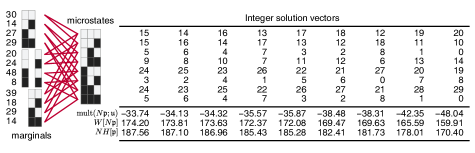
Figure 1: From marginal constraints to integer solutions of the linear system: Bipartite graph representation of coefficient matrix $\mathbf{C}$ relating the vector of marginals to the microstate probabilities. On the leftmost, marginal frequencies are provided as input. Boxes refer to feature 1,2, and 3, where white color indicates $\alpha_{i}=0$ and black $\alpha_{i}=1$. Microstates are represented in the same fashion. Table gives the solution set of the Diophantine system consisting of column vectors of counts for all microstates. For each solution vector, three metrics are listed: the logarithm of multinomial probability and multinomial coefficient as well as $N=100$ times entropy.

The solution in the top row not only has the highest ($\log$) likelihood among the solution set, but is also the one which can be realized in the most ways displaying the highest entropy. Evidently, the rational-valued $\mathfrak{p}$ at the top of Table 1b does not necessarily coincide with the maxent solution on the simplex Eq. (2) under pairwise constraints. Maximizing the entropy functional defined over the one-dimensional solution space associated to Eq. (8) in the present setting yields the optimal, real-valued distribution $\hat{\mathfrak{p}}\in[\mathfrak{f}]$. Its entries are given on the rightmost of Plot 2a. Rounding all entries of the real-valued vector $100\hat{\mathfrak{p}}$ to the nearest integer recovers the most probable solution at the top of Table 1b. Already at a sample size of $N=100$, the entropy $H[\mathfrak{p}]$ can well approximate $N^{-1}\log W[N\mathfrak{p}]$ with a relative error of $\mathcal{O}\left(10^{-1}\right)$. Hence, our conclusion about $\hat{\mathfrak{p}}$ as the asymptotic solution that is most likely and realized in the most possible ways remains unaltered. In a generic setting, it quickly becomes [28] computationally infeasible to determine all solutions of the Diophantine linear system or analytically solve entropy extremization in $[\mathfrak{f}]$ for $\hat{\mathfrak{p}}$, so that iterative methods directly yielding the limiting distribution become indispensable.

An iterative method based on some parametric ansatz requires to first choose an encoding for the feature realizations such that a non-redundant set of independent parameters can be defined in order to estimate the maxent distribution $\hat{\mathfrak{p}}$. By contrast, we apply ipf directly on the $D=12$ marginal relative frequencies in all two-clusters requiring only to arbitrarily fix an ordering of microstates in $\mathcal{A}$ and of the rational-valued marginal constraints $\{\widehat{m}_{a}\}_{a=1,...,D}$. Let us first see how to estimate the probability of microstate $(0,0,0)$ for which the initial uniform probability of $\mathfrak{p}^{(0)}(0,0,0)=1/8$ deviates from the maxent value $\hat{\mathfrak{p}}(0,0,0)\approx 0.149276$ by more than $16\%$. In the first cycle, we start by applying Eq. (18) on feature pair $\{1,2\}$:

$$\mathfrak{p}^{(1)}(0,0,0)=\mathfrak{p}^{(0)}(0,0,0)\frac{\mathfrak{f}_{12}(0,0)}{\mathfrak{p}^{(0)}(0,0,0)+\mathfrak{p}^{(0)}(0,0,1)}=\frac{3}{20}~{}~{}, ~{}~{}\mathfrak{p}^{(1)}(0,1,0)=\mathfrak{p}^{(0)}(0,1,0)\frac{\mathfrak{f}_{12}(0,1)}{\mathfrak{p}^{(0)}(0,1,0)+\mathfrak{p}^{(0)}(0,1,1)}=\frac{7}{100}~{},$$

$$\mathfrak{p}^{(1)}(1,0,0)=\mathfrak{p}^{(0)}(1,0,0)\frac{\mathfrak{f}_{12}(1,0)}{\mathfrak{p}^{(0)}(1,0,0)+\mathfrak{p}^{(0)}(1,0,1)}=\frac{27}{200}~{}, ~{}~{}\mathfrak{p}^{(1)}(1,1,0)=\mathfrak{p}^{(0)}(1,1,0)\frac{\mathfrak{f}_{12}(1,1)}{\mathfrak{p}^{(0)}(1,1,0)+\mathfrak{p}^{(0)}(1,1,1)}=\frac{29}{200}~{}.$$

The estimated probabilities of microstates $(0,1,0)$, $(1,0,0)$ and $(1,1,0)$ are needed for the next steps of the cycle. Proceeding with the subsets $\{1,3\}$ and $\{2,3\}$ we compute

$$\mathfrak{p}^{(2)}(0,0,0)=\mathfrak{p}^{(1)}(0,0,0)\frac{\mathfrak{f}_{13}(0,0)}{\mathfrak{p}^{(1)}(0,0,0)+\mathfrak{p}^{(1)}(0,1,0)}=\frac{3}{22}~{}, \mathfrak{p}^{(2)}(1,0,0)=\mathfrak{p}^{(1)}(1,0,0)\frac{\mathfrak{f}_{13}(1,0)}{\mathfrak{p}^{(1)}(1,0,0)+\mathfrak{p}^{(1)}(1,1,0)}=\frac{81}{350}\phantom{\hskip 7.96674pt,}$$

and $$\mathfrak{p}^{(3)}(0,0,0)=\mathfrak{p}^{(2)}(0,0,0)\frac{\mathfrak{f}_{23}(0,0)}{\mathfrak{p}^{(2)}(0,0,0)+\mathfrak{p}^{(2)}(1,0,0)}=\frac{273}{1888}~{},$$

respectively. The estimate $\mathfrak{p}^{(3)}(0,0,0)$ in the last step of the first cycle deviates from the actual maxent $\hat{\mathfrak{p}}(0,0,0)$ by $3\%$ improving our naive uniform guess by more than $13\%$. The ipf estimation of all $\mathfrak{p}_{\alpha}$’s over the first four cycles is depicted in Figure 2a. As the effect of applying marginal constraints over the first cycle is stronger, quickly becoming small in later cycles, we have used a logarithmic scale to increase visibility. In the lower part, we plot (also in logarithmic scale) the kl divergence of the ipf estimate from limiting distribution $\hat{\mathfrak{p}}$ to exemplify how the running estimate of the iterative procedure approaches the asymptotic distribution. After having deduced the maxent distribution $\hat{\mathfrak{p}}$ from the summary statistics of marginal vector $\widehat{m}$, one can compute various metrics. In particular, from the log-odds

$$h_{1}=\log\frac{\hat{\mathfrak{p}}(1,0,0)}{\hat{\mathfrak{p}}(0,0,0)}\approx 0.478\quad \quad h_{2}=\log\frac{\hat{\mathfrak{p}}(0,1,0)}{\hat{\mathfrak{p}}(0,0,0)}\approx 1.079\quad \quad h_{3}=\log\frac{\hat{\mathfrak{p}}(0,0,1)}{\hat{\mathfrak{p}}(0,0,0)}\approx 0.01$$

$$J_{12}=\log\frac{\hat{\mathfrak{p}}(1,1,0)}{\hat{\mathfrak{p}}(0,1,0)}-h_{1}\approx 1.073\quad \quad J_{13}=\log\frac{\hat{\mathfrak{p}}(1,0,1)}{\hat{\mathfrak{p}}(0,0,1)}-h_{1}\approx-2.117\quad \quad J_{23}=\log\frac{\hat{\mathfrak{p}}(0,1,1)}{\hat{\mathfrak{p}}(0,0,1)}-h_{2}\approx 0.556$$

one recovers a familiar-looking description [29] – dating back to the well-known Ising model [30] – of the maxent distribution defined by pairwise marginal constraints, in terms of interaction matrix $\mathbf{J}$ and bias vector $\vec{h}$. Those metrics correspond to the Lagrange multipliers that incorporate a minimal set of $d-1=6$ marginal constraints in the exponential family of distributions.

Figure 2: Evolution of the estimate for $\hat{\mathfrak{p}}$ during the first 4 cycles of ipf algorithm: (a) Probabilities of microstates as estimated by ipf, starting from the uniform ansatz $\mathfrak{u}(\alpha_{1},\alpha_{2},\alpha_{3})=1/8$ and fitting empirical relative marginals $\mathfrak{f}_{ij}(\alpha_{i},\alpha_{j})$ deduced from Figure 1 in all pairs of features $\{1,2\}$, $\{1,3\}$ and $\{2,3\}$. The asymptotic values of $\hat{\mathfrak{p}}(\alpha_{1},\alpha_{2},\alpha_{3})$ are given rounded on the rightmost. (b) kl divergence of estimated distribution after each step from the limiting maxent distribution $\hat{\mathfrak{p}}$.

We have demonstrated that a parameter-free problem formulation together with the compatibly parameter-agnostic ipf recovers the model distribution $\hat{\mathfrak{p}}$ of maximal entropy that satisfies all marginal constraints provided in the problem statement. Having the optimal solution $\hat{\mathfrak{p}}$ at hand, the optimal values of parameters in any meaningful parametrization can be calculated. This clearly demonstrates that the notion of parameters is not required for the definition and estimation of $\hat{\mathfrak{p}}$. Not only are parametric models superfluous, their application is restricted to distributions in the exponential family, rendering the estimation of distributions with structural zeros cumbersome. Thus, our ansatz is much more general than any parametric model. In this context, ipf becomes a uniquely flexible iterative estimator, because its application only requires a consistent set of marginal constraints in arbitrary subsets of $L$ features, whose information is iteratively incorporated into the model distribution.

5 Application

During the analysis of real-world data we are inevitably confronted with the pitfalls of a finite sample that could distort the picture we deduce about the population the sample descended from. In our setting, a sampled dataset is naturally described by a set of marginal constraints (i.e. empirical relative frequencies) from the sample’s empirical distribution. Generically, larger sample sizes tend to increase our trust on marginal constraints in larger subsets of features. Choosing marginal relative frequencies from the provided data matrix $\mathbf{X}$ as constraints, automatically selects also candidates for associations, because all unspecified or unimplied marginal constraints lead to the absence of the corresponding associations in the model, i.e. the generalized odds ratios correspondingly equal unity. In the following, we shall assume for concreteness that any comprehensive set of marginal probabilities $\widehat{m}$ calculated from the data $\mathbf{X}$ consists of marginal distributions in clusters of features. The cardinality of a cluster defines the order of the marginal distribution which points to the order of association among the features.

In a fully data-driven spirit, there is ground to neither postulate nor exclude any pair-wise or higher-order associations. In principle, one would need to investigate any possible set of marginal constraints that could be computed from $\mathbf{X}$. Since the powerset of $L$ features includes $2^{L}-1$ non-empty clusters, we anticipate at most $2^{2^{L}-1}$ sets of clusters of features, but symmetries among marginal distributions massively reduce this number. By comparing the maxent distributions derived from summary statistics over the various sets of constraints, the minimal set of marginal distributions required to accurately capture all major trends in the population can be found. We demonstrate modeling of real-world data and propose how to choose a set of constraints at the level of marginal distributions that can lead to the most accurate description of population statistics based on samples of a given size. To select one of the admissible sets of marginal constraints that would lead to a faithful description of the data we use an approach inspired by subsampling [31] and the bootstrap [32].

Specifically, let us consider a fictitious infinite population. Within the state space $\mathcal{A}$ this “population” has (definite and known) microstate distribution coinciding with the empirical distribution $\mathfrak{f}$ from the provided sample. Thus, we assume an asymptotic distribution, which is in general expected to contain any possible associations. Subsequently, we sample from this “population” multiple datasets $s$ of various sizes resulting in sample distributions $\mathfrak{f}^{(s)}$ and compute the maxent distributions $\hat{\mathfrak{p}}^{(s,k)}$ associated to the equivalence classes $[\mathfrak{f}^{(s)}]_{k}$ for all distinct summary statistics of each sample $s$ enumerated by $k$. Intuitively, our aim is to select the summary statistics $k^{*}$ which leads to model distribution $\hat{\mathfrak{p}}^{(s,k^{*})}$ that is closest to the “population” distribution $\mathfrak{f}$ of microstates. The distance of model distribution $\hat{\mathfrak{p}}^{(s,k)}$ from $\mathfrak{f}$ is naturally quantified by the kl divergence

$$D_{\textsc{kl}}(\mathfrak{f}\;\|\;\hat{\mathfrak{p}}^{(s,k)})=-H[\mathfrak{f}]-\sum_{\alpha=1}^{\left|\mathcal{A}\right|}\mathfrak{f}_{\alpha}\log\hat{\mathfrak{p}}^{(s,k)}_{\alpha}~{},$$

which essentially measures the opposite of the likelihood of the empirical distribution under the given model (the entropy of the provided dataset being constant). In this context, it becomes reasonable to regularize subsample distributions $\mathfrak{f}^{(s)}$ by adding a pseudocount of unity to all admissible microstates, as discussed in A, in order to ensure that the relative frequencies observed in $\mathfrak{f}$ remain also non-zero in $\mathfrak{f}^{(s)}$ thus preventing infinite kl divergences.

To demonstrate the fully data-driven reasoning, we have considered all entries documented over the years 2003 - 2018 at the emergency department (ed) by the National Hospital Ambulatory Medical Care Survey (nhamcs) from the public database of the National Center for Health Statistics. Datasets and documentation can be downloaded from https://www.cdc.gov/nchs/ for public use. We have concentrated on patients whose fate is known, excluding anyone who either left against medical advice or left without being seen or before treatment completion. In addition, anyone who arrived already dead at the ed was excluded. In this way, $N=392\,454$ records remained from which $44\,293$ were admitted to hospital. A case is considered critical whenever the patient was admitted to an intensive/critical care unit (icu) or died during the hospital stay resulting in $6\,300$ critical cases out of $44\,293$ hospitalized patients. Here, we encounter a structural zero, because non-hospitalized but critical patients are obviously impossible. Despite the fact that structural zeros are often encountered in realistic settings signifying associations that are deterministically forbidden, it is common practice to either adjust a parametric model accordingly to ensure that estimation remains possible or (more alarmingly) features are removed. Our ansatz requires neither a change in the model nor to the data, whenever structural zeros are present.

In detail, we choose to work with $L=4+1$ categorical features with $\vec{q}=\left(6,2,2,2,2\right)$ from the original dataset: age group, sex, arrival by ambulance and hospitalization augmented by the dimension of criticality defined in the previous paragraph. In the microstate space of ${\left|\mathcal{A}\right|}=6\cdot 2\cdot 2\cdot 2\cdot 2=96$ microstates (the counts are given in Supplementary Table S1), only $|\mathcal{A}^{\prime}|=96-6\cdot 2\cdot 2\cdot 1=72$ are not associated with the aforementioned structural zero. To get a feeling about marginal constraints that reflect actual associations in the population beyond finite sampling effects, we first examine models incorporating the observed marginal distributions in all clusters of features of a given cardinality $\ell$, which we refer to as the order of summary statistics. In principle, we have to estimate 5 maxent distributions corresponding to summary statistics of orders $\ell=1,2,3,4,5$, but in the reduced state space $\mathcal{A}^{\prime}$ the equivalence class $[\mathfrak{f}]_{\ell=4}$ incorporating all fourth-order marginal distributions coincides with $[\mathfrak{f}]_{\ell=5}=\{\mathfrak{f}\}$. To non-trivially obtain any model distribution $\mathfrak{p}^{(s,\ell)}$ we apply ipf using summary statistics of the desired order.

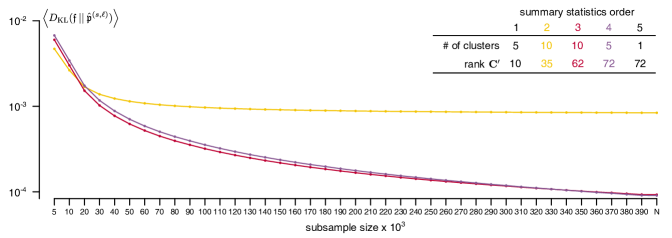
Figure 3: Average kl divergence from empirical distribution $\mathfrak{f}$ of models $\hat{\mathfrak{p}}^{(s,\ell)}$ (in $\log$ scale). maxent distributions $\hat{\mathfrak{p}}^{(s,\ell)}$ are constructed on $20\,000$ datasets subsampled for each of the sample sizes indicated on the x-axis. The colors indicate models incorporating all two- (yellow), three- (red), and four-order (purple) empirical marginal distributions. The $\ell=1$ model is not displayed for clarity, as it constitutes a poor fit for $\mathfrak{f}$. The rank of the reduced coefficient matrix is conventionally referred to as the dimension of the model.

After sampling $20\,000$ datasets for each subsample size ranging from $5\,000$ up to $N$, we averaged the kl divergence of the model $\hat{\mathfrak{p}}^{(s,\ell)}$ from “population” distribution $\mathfrak{f}$ over all samples of a given size for the orders of summary statistics leading to distinct models, as depicted in Figure 3.

The average kl divergence for $\ell=1$ remains at all subsample sizes very large signifying that the corresponding maxent model cannot accommodate major trends in the empirical distribution as satisfactory as higher-order models. Since summary statistics of order $\ell=1$ imply independence between the features, this indicates the presence of at least one higher-order association (already anticipated by the presence of structural zero) between the features which is necessary to describe the “population” distribution $\mathfrak{f}$. More interestingly, the average kl divergence for $\ell=2$ at subsample sizes below $20\,000$ was smaller than for $\ell=3,4$. Model distributions $\hat{\mathfrak{p}}^{(s,2)}$ tend on average to describe the “population” distribution $\mathfrak{f}$ better than more complex models at those smaller sample sizes, since there is only limited evidence from the data for higher-order associations. Starting at subsample sizes of $20\,000$ up to $340\,000$ the average kl divergences signify that the maxent distributions deduced from $[\mathfrak{f}^{(s)}]_{\ell=3}$ constitute optimal fits for the “population” distribution $\mathfrak{f}$. Only at sample sizes larger than $340\,000$ ($>89$% of the nhamcs original size) the average kl divergence of $\ell=4$ model becomes the lowest. Notice that even at $\mathcal{O}\left(N\right)$ sample sizes the maxent model deduced from summary statistics of cubic order performs on a comparable scale to the maxent model deduced from summary statistics of quartic order, which is the same as directly using $\mathfrak{f}^{(s)}$.

In total, we acknowledge that it would have been difficult to identify higher-order associations, although they are clearly present in the “population” distribution $\mathfrak{f}$, if the sample size of the nhamcs dataset were considerably low. On the other hand, at least third-order summary statistics seem to be required given enough data to achieve a better description of the fictitious population, as the pairwise model consistently fails to approach $\mathfrak{f}$ over a wide range of larger subsample sizes. As the sample size approaches $N$, at least one fourth-order effect may be identifiable. However, the observation that the maxent model deduced from marginal constraints on all clusters of carnality $\ell=3$ performs almost equally well to the one when $\ell=4$ suggests that not all quartic-order associations might be needed to faithfully depict the target distribution $\mathfrak{f}$.

To test whether the specification of all empirical marginal distributions in four-clusters is actually required, we now investigate via our bootstrap scheme all possible summary statistics where each of the $L=5$ features belongs to at least one cluster, resulting in a total of $6\,893$ sets of constraints. Calculating each set of marginal distributions $k=1,\ldots,6\,893$ on each dataset $s=1,\ldots,20\,000$ of size $N$ sampled from the empirical $\mathfrak{f}$ of the original nhamcs data, we consider again the kl divergence of the deduced maxent distribution $\hat{\mathfrak{p}}^{(s,k)}$ from $\mathfrak{f}$. Since the kl divergences of the models in a given sample $s$ are linked via the sample they were estimated from, we compared the kl divergence from $\mathfrak{f}$ of the maxent distributions $\hat{\mathfrak{p}}^{(s,k)}$ to the one of the sample $\mathfrak{f}^{(s)}$ itself, by computing their respective difference. This difference is positive whenever $\mathfrak{f}^{(s)}$ is closer to $\mathfrak{f}$ than any non-trivial model $\hat{\mathfrak{p}}^{(s,k)}$ and attains negative values whenever the sample distribution lies further away (Figure 4a). Even at sample sizes of order $N$, our analysis reveals that there remain sets of constraints that perform consistently better than trivially using the empirical distribution $\mathfrak{f}^{(s)}$ of each sample to describe $\mathfrak{f}$.

Taking a closer look at the sets of marginal constraints outperforming on average the sample distribution, we detect two groups of summary statistics. Within the first group that scores best for instance, there exist 13 sets of marginal distributions (summarized by hypergraphs in Figure 4b) resulting in the same maxent distribution $\hat{\mathfrak{p}}^{(s,k)}=\mathfrak{q}^{(s)}$ for $k=1,\ldots,13$. In fact, such degeneracy at the level of hypergraphs representing clusters of features is to be expected and goes beyond the maxent logic dictating the optimal distribution. The linear systems Eq. (8) induced by any of these sets of constraints coincide, as it can be immediately recognized by computing the reduced row echelon form of their coefficient matrices leading to full equivalence of the hypergraphs at the level of the induced equivalence class Eq. (7). In principle, the reduced row echelon form of the augmented matrix had to be invoked in order to conclude on the equivalence of linear systems. However, we know that our linear systems generically have by construction infinitely many solutions, hence augmenting the (reduced) coefficient matrix by the vector of empirical marginal sums does not add any new dimension to the span of columns.

Starting from any of the sets of marginal constraints represented by the 13 hypergraphs, it is instructive to distinguish the invariant part defining the same equivalence class that leads to $\mathfrak{q}^{(s)}\in[\mathfrak{f}^{(s)}]$ from the redundant specification in terms of marginals (left column in Figure 4c depicted for the first hypergraph of 4b). The row reduction of the architecture matrix $\mathbf{C}^{\prime}$ that describes one of the sets of redundant constraints correspondingly induces a row reduction of the marginal vector $\widehat{m}$ leading to a set of $\text{rank}\,\mathbf{C}^{\prime}=66$ generalized marginal constraints (middle column in Figure 4c) that comprise the linearly independent rules to be obeyed by any $\mathfrak{p}\in[\mathfrak{f}^{(s)}]$. Note that in the dual formulation, the non-vanishing generalized marginal constraints would be enforced by Lagrange multipliers (as outlined in C) acquiring the role of parameters.

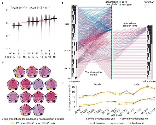
Figure 4: Selection of the best fitting model. (a) Difference between the kl divergences from $\mathfrak{f}$ of a model $\hat{\mathfrak{p}}^{(s,k)}$ and of $\mathfrak{f}^{(s)}$ is computed over 20 000 samples. Depicted are the ten top ranking models being closest to $\mathfrak{f}$. The $\ell=3,4$ models from Figure 3 are signified by red and purple color, respectively. Each model can be defined via multiple sets of marginal constraints. (b) Hypergraph representation of the set of feature-clusters for which empirical marginal distributions are specified as input. All 13 hypergraphs depicted here lead to identical linear systems and maxent distribution with the best score in (a). (c) Left column represents the realizations of marginal distributions in the clusters from the first hypergraph in (b). Via Gaussian elimination we obtain the middle column of generalized marginal constraints. The reduced row echelon form relates the non-vanishing generalized marginals (denoted by green) to the probabilities of microstates in the right column. (d) Conditional probabilities given patient’s age, sex and means of arrival at the hospital computed from the best-scoring model in (a), the empirical distribution (purple) and the pairwise model (yellow) of Figure 3.

Having seen that there exist sets of marginal constraints leading to a model distribution $\mathfrak{q}$ that describes better the “population” distribution $\mathfrak{f}$ starting from its samples $\mathfrak{f}^{(s)}$ than using $\mathfrak{f}^{(s)}$ itself, allows us to conclude that any additional empirical constraint at sample sizes of order $N$ cannot be resolved against sampling noise and should be thus omitted. Once $\mathfrak{q}\in[\mathfrak{f}]$ is deduced, it can be used to compute association metrics of biomedical interest, such as conditional probabilities and odds ratios. For example, the prediction of critical cases given patient’s profile and means of arrival is plotted in Figure 4d using model $\mathfrak{q}$ which scores best in the bootstrap. To compare the effect of constraint selection on the predictive power of a model, we also include the same conditional probabilities deduced from the empirical distribution $\mathfrak{f}$ as well as from the frequently used “baseline” model of pairwise summary statistics (yellow model in Figure 3). The simpler model of pairwise associations entirely fails to differentiate the age profile by means of arrival (arriving by ambulance results in a mere increase of conditional probability over all age groups by the same amount). Whereas the most complex model induced by $\mathfrak{f}$ itself seems to mostly perform on a comparable scale to $\mathfrak{q}$, as anticipated by subsampling scheme in Figure 4a, it overestimates the risk of arrival by ambulance especially for female younger patients by more than $1.5\%$.

In summary, our problem formulation allowed us to minimally determine sets of phenomenological constraints which go beyond pairwise associations in order to faithfully depict the original dataset. Furthermore, it clearly pointed towards optimal sets of constraints selecting a model distribution that describes the wealth of associations as good as using the empirical distribution itself, while excluding any effects that are indistinguishable from sampling noise at the given sample size. Analysing the architecture matrix uncovered the degeneracy of hypergraphs in any group of summary statistics which behave identically in our comparison tests, demonstrating that in presence of structural zeros naively enumerating hypergraphs specifying marginal distributions in clusters of features is not enough to filter out all degeneracies. Only linear system Eq. (8) gives a conclusive verdict on distinct sets of marginal constraints which are expected to lead to generically distinct maxent distributions giving a straight-forward classification of inequivalent constraints and hence a robust model definition. To arrive at any model distribution neither the data from nhamcs nor the algorithmic procedure of modeling had to be adjusted. The implementation of ipf at the level of probabilities $\mathfrak{p}_{\alpha}$ helps efficiently obtain any distribution given empirical constraints without the need to tackle awkward parametrizations. All in all, the outlined analysis constitutes a purely data-driven approach that can accommodate any class of multivariate categorical distributions with profound consequences in the area of machine learning.

Acknowledgments

We are thankful to Alan Race for useful discussions and proof-reading the manuscript. Furthermore, we thank Jan-Bernhard Kordaß for useful comments on the original arxiv version.

Appendix A Modeling finite populations

In the setting of categorical features, observed counts $N\mathfrak{f}_{\alpha}$ are to be sampled under some model $\mathfrak{q}$ via a hypergeometric distribution. For sufficiently large populations, it is permissible [36] to use instead of the hypergeometric the multinomial distribution. Treating a population as a pool with infinitely many individuals to sample from is evidently an idealization. For the purposes of modeling and benchmarking however, this simplifying approximation is mostly sufficient. To convince ourselves we consider in Plot 5 the simplistic example of a two-dimensional space $\mathcal{A}=\{\text{success},\text{failure}\}$ with $K=400$ cases of success in a finite population of $M=1\,000$ individuals. We perform an experiment with $N=100$ trials and ask about the observed count $n$ of successes. Immediately, we recognize that hypergeometric distribution $H(n;M,K,N)$ when sampling without replacement and binomial distribution $B(n;N,q)$ when sampling with replacement using $q=K/M=2/5$ exhibit very similar profiles, even in a smaller population. To compare with the entropy-based analysis advocated in this paper, we also plot (in purple) the information-theoretic approximation to multinomial distribution,

$$\log\text{mult}(N\mathfrak{f};\mathfrak{q})=-ND_{\textsc{kl}}(\mathfrak{f}\;\|\;\mathfrak{q})-\frac{\left|\mathcal{A}\right|-1}{2}\log N+\mathcal{O}\left(1\right)~{}.$$ (21)

in terms of the kl divergence of model $\mathfrak{q}=(q,1-q)$ from the observed counts $N\mathfrak{f}=(n,N-n)$.

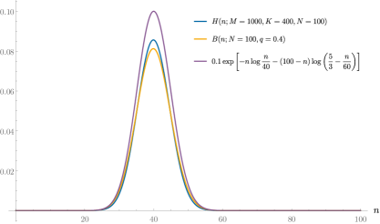
Figure 5: Comparative plot of the count $n$ of successes as observed in a sample of size $100$ following a hypergeometric distribution $H$ as well as its binomial counterpart $B$ with the information-theoretic approximation Eq. (21). In the population of $1\,000$ individuals there are $400$ cases of success.

Pseudo-count regularization.

In real life, data usually comes at a limited number of samples with the result that certain microstates in $\mathcal{A}$ with low probabilities remain unobserved in a finite dataset of size $N$, especially whenever the distribution strongly picks around some other region in microstate space. To avoid erroneous singularities in information-theoretic metrics such as the kl divergence, it thus becomes eminent the need to regularize so that the data-driven analysis captures – as much as possible – the physically relevant behavior of the underlying system. Theoretically, it is reasonable to assume that any configuration in $\mathcal{A}^{\prime}$ is possible, $\mathfrak{p}_{\alpha}\neq 0$ if not otherwise stated, anticipating finite associations among features. To roughly compensate for unobserved configurations, so-called sampling zeros, one can employ [37] the pseudo-count method. Following the logic of a least-biased setup each configuration $\alpha$ (except for those associated to any structural zero) uniformly receives a pseudo-count, before seeing the actual data. In other words, one works with a slightly modified empirical distribution

$$\mathfrak{f}_{\alpha}\quad\rightarrow\quad\frac{1}{1+\lambda/N\cdot\left|\mathcal{A}^{\prime}\right|}\left[\lambda/N+\mathfrak{f}_{\alpha}\right]$$ (22)

for some real $\lambda>0$, which in turn implies for its summary statistics

$$\widehat{m}_{a}\quad\rightarrow\quad\frac{1}{1+\lambda/N\cdot\left|\mathcal{A}^{\prime}\right|}\left[\frac{\lambda}{N}\sum_{\alpha=1}^{\left|\mathcal{A}^{\prime}\right|}C^{\prime}_{a\alpha}+\widehat{m}_{a}\right]~{}.$$ (23)

The effective regularization strength $\lambda/N$ is a – hopefully small – hyper-parameter to be tuned depending on the application field. Generically for larger data sets of size $N$, it can be taken at order $1/N$. This simple prescription helps us avoid any erroneous (near)-singular behavior that would appear whenever some entry of marginal vector $m_{a}$ happens to be close to zero – meaning that all affected relative frequencies $\mathfrak{f}_{\alpha}$ and estimates of ipf update rule thereof, would be immediately set to zero.

Models with uniform summary statistics.

Let us give an explicit formula for the dimension of the linear problem $d=\text{rank}\,\mathbf{C}$ in absence of any structural zero marginal relative frequency $\widehat{m}_{a}$, i.e. when $\mathcal{A}^{\prime}=\mathcal{A}$. For concreteness, we uniformly specify marginal distributions in all

$$\sum_{a=1}^{D}C_{a\alpha}=\begin{pmatrix}L\\ \ell\end{pmatrix}$$

subsets of cardinality $\ell$ leading to

$$D=\sum_{i_{1}=1}^{L}q_{i_{1}}\sum_{i_{2}>i_{1}}^{L}q_{i_{2}}\cdots\sum_{i_{\ell}>i_{\ell-1}}^{L}q_{i_{\ell}}$$

– in principle redundant – constraint equations. Considering pairwise summary statistics for example, the set of induced marginal constraints in a two-cluster $\{i,j\}$ explicitly constitutes $q_{i}\times q_{j}$ redundant equations. Summing either over the $j$-th or $i$-th direction leads to the constraint equations corresponding to one-feature marginal distribution $\mathfrak{f}_{i}(\alpha_{i})$ and $\mathfrak{f}_{j}(\alpha_{j})$, respectively. However, these one-site constraints would be also obtained from summing over any other two-feature marginal distributions $\mathfrak{f}_{ik}(\alpha_{i},\alpha_{k})$ and $\mathfrak{f}_{jk}(\alpha_{j},\alpha_{k})$ with $k\neq i,j$. To avoid overcounting constraints we thus need to effectively reduce the Potts order $q_{i}$ of features. Indeed, regarding one-feature marginal distributions as given for $i,j=1,\ldots,L$ only $(q_{i}-1)\times(q_{j}-1)$ from the $q_{i}\times q_{j}$ constraint equations in the cluster $\{i,j\}$ are independent. In turn, there are only $q_{i}-1$ independent constraints induced by $\mathfrak{f}_{i}(\alpha_{i})$, as one is implied by the others in conjunction with normalization on the simplex $\mathcal{P}$. Counting independent constraints in that way readily generalizes to $\nu$-th order summary statistics, where $\left(q_{i_{1}}-1\right)\times\cdots\times\left(q_{i_{\nu}}-1\right)$ independent conditions in each subset $\{i_{1},...,i_{\nu}\}\subset\{1,...,L\}$ are anticipated. In total, out of the $D$ consistent equations only

$$d=1+\sum_{\nu=1}^{\ell}\sum_{i_{1}<...<i_{\nu}}\left(q_{i_{1}}-1\right)\cdots\left(q_{i_{\nu}}-1\right)$$

constraints are independent representing independent information from empirically observed data matrix $\mathbf{X}$.

Appendix B Convergence of IPF and unique existence of MaxEnt distribution

In the first section of this paper, we have seen that the phenomenological constraints imposed by marginal relative frequencies from a data matrix $\mathbf{X}$ together with the optimality goal of mle defined a linear program. Summarizing:

Program 1.

The maxent distribution $\hat{\mathfrak{p}}$ is obtained as the optimal solution to linear program

$$\min_{\mathfrak{p}\in\mathbb{R}^{\left|\mathcal{A}\right|}}\sum_{\alpha=1}^{\left|\mathcal{A}\right|}\mathfrak{p}_{\alpha}\log\mathfrak{p}_{\alpha}\quad\text{subject to}\quad\sum_{\alpha=1}^{\left|\mathcal{A}\right|}C_{a\alpha}\,\mathfrak{p}_{\alpha}=\widehat{m}_{a}~{}\text{ for }~{}a=1,...,D\quad\text{and}\quad\mathfrak{p}_{\alpha}\geq 0~{}\text{ for }~{}\alpha=1,...,{\left|\mathcal{A}\right|}~{}.$$

Evidently, the feasible region of linear program 1, coinciding with the equivalence class $[\mathfrak{f}]$ of all distributions compatible with marginals $\widehat{m}$, is non-empty provided a consistent set of phenomenological constraints. Next, we turn to optimality to assert the asymptotic existence of the maxent solution. Note that uniqueness immediately follows from existence, as entropy is strictly concave (equivalently $D_{\textsc{kl}}(\mathfrak{p}\;\|\;\mathfrak{u})$ is strictly convex) in $\mathfrak{p}\in[\mathfrak{f}]$ and hence possesses at most one global maximum (equivalently minimum of kl divergence) in the convex set spanned by the equivalence class. All in all, we have

Theorem 3.

Among all distributions $\mathfrak{p}$ in the equivalence class $[\mathfrak{f}]$ induced by marginal probabilities $m\overset{!}{=}\widehat{m}$ there always exists a unique probability distribution $\hat{\mathfrak{p}}$ having the maximum entropy in the given equivalence class, $\hat{\mathfrak{p}}=\max\limits_{\mathfrak{p}\in[\mathfrak{f}]}H[\mathfrak{p}]$.

Showing the existence of maxent distribution in $[\mathfrak{f}]$ amounts to proving the convergence of ipf algorithm to $\hat{\mathfrak{p}}$. In order to do so we need a base Lemma from probability theory which says that

Lemma 1.

If $\hat{\mathfrak{p}}\in\mathcal{P}$ is maxent distribution in an equivalence class $[\mathfrak{f}]$, then

$$H[\hat{\mathfrak{p}}]\geq H[\mathfrak{p}]~{}\forall\,\mathfrak{p}\in[\mathfrak{f}]\quad\Leftrightarrow\quad D_{\textsc{kl}}(\mathfrak{p}\;\|\;\hat{\mathfrak{p}})=H[\hat{\mathfrak{p}}]-H[\mathfrak{p}]\quad\Leftrightarrow\quad\sum_{\alpha=1}^{\left|\mathcal{A}\right|}\left(\mathfrak{p}_{\alpha}-\mathfrak{\hat{\mathfrak{p}}}_{\alpha}\right)\log\hat{\mathfrak{p}}_{\alpha}=0~{}.$$

In fact, this is a special case of the analogue of Pythagorean theorem for kl divergences, see e.g. [38, 39]. To prove the forward direction of the equivalence we introduce a family of parametric functions on $\mathbb{R}$ via

$$\mathfrak{s}_{\alpha}(\lambda)=\lambda\mathfrak{p}_{\alpha}+\left(1-\lambda\right)\hat{\mathfrak{p}}_{\alpha}\quad\text{for}\quad\alpha=1,...,{\left|\mathcal{A}\right|}~{}.$$ (24)

For each microstate from $\mathcal{A}$ our function $\mathfrak{s}_{\alpha}(\lambda)$ describes a line with slope $\mathfrak{p}_{\alpha}-\hat{\mathfrak{p}}_{\alpha}$ and either positive or zero intercept $\hat{\mathfrak{p}}_{\alpha}$. In the latter case, $\alpha$ belongs to the complement of realization space $\mathcal{A}^{\prime}$ and the slope becomes also zero, hence $\mathfrak{s}_{\alpha}(\lambda)=0$ for any $\lambda$. In the former scenario of positive intercept, we know by continuity of the straight line that there is always a finite region around $\lambda=0$ where $\mathfrak{s}_{\alpha}$ remains non-negative. In total, there should always exist some $t>0$ such that $\mathfrak{s}_{\alpha}(\lambda)$ is non-negative when $\lambda\in(-t,t)$ for all realizations in $\mathcal{A}$ indexed by $\alpha$. Furthermore, being a linear combination of $\hat{\mathfrak{p}},\mathfrak{p}\in[\mathfrak{f}]$ the vector $\mathfrak{s}(\lambda)$ parametrized by $\lambda\in(-t,t)$ automatically satisfies the linear constraints and represents thus a distribution $\mathfrak{s}(\lambda)\in[\mathfrak{f}]$. From Lemma 1 we then have

$$H[\hat{\mathfrak{p}}]\geq H[\mathfrak{s}(\lambda)]$$ (25)

for those $\lambda$ around $\lambda=0$ where $\mathfrak{s}_{\alpha}(\lambda)\geq 0~{}\forall\alpha$, implying in particular that

$$f(\lambda)\equiv\sum_{\alpha=1}^{\left|\mathcal{A}\right|}\mathfrak{s}_{\alpha}(\lambda)\log\mathfrak{s}_{\alpha}(\lambda)-\sum_{\alpha=1}^{\left|\mathcal{A}\right|}\hat{\mathfrak{p}}_{\alpha}\log\hat{\mathfrak{p}}_{\alpha}\geq 0~{}.$$ (26)

The strictly convex function $f$ attains its minimum at $\lambda=0$ as $\hat{\mathfrak{p}}$ is assumed to be maxent in $[\mathfrak{f}]$. By the derivative condition we immediately get the desired identity:

$$0\overset{!}{=}\left.\frac{\text{d}f(\lambda)}{\text{d}\lambda}\right|_{\lambda=0}=\sum_{\alpha=1}^{\left|\mathcal{A}\right|}\left(\mathfrak{p}_{\alpha}-\hat{\mathfrak{p}}_{\alpha}\right)\log\hat{\mathfrak{p}}_{\alpha}~{}.$$ (27)

Proving the opposite direction is more straight-forward. Starting from the re-arranged expression

$$-\sum_{\alpha=1}^{\left|\mathcal{A}\right|}\hat{\mathfrak{p}}_{\alpha}\log\hat{\mathfrak{p}}_{\alpha}=-\sum_{\alpha=1}^{\left|\mathcal{A}\right|}\mathfrak{p}_{\alpha}\log\hat{\mathfrak{p}}_{\alpha}$$ (28)

we subtract from both sides $H[\mathfrak{p}]$ so that

$$H[\hat{\mathfrak{p}}]-H[\mathfrak{p}]=D_{\textsc{kl}}(\mathfrak{p}\;\|\;\hat{\mathfrak{p}})\geq 0$$ (29)

with equality only when $\mathfrak{p}=\hat{\mathfrak{p}}$. Thus, $\hat{\mathfrak{p}}$ has the maximum entropy in $[\mathfrak{f}]$.

In this work, we have advocated the use of ipf algorithm to obtain the maxent distribution from empirical marginal constraints working exclusively in the space of physically meaningful probabilities. At the $(n+1)$-th cycle after fitting onto marginal distribution in the subset $\{i_{1},\ldots,i_{\ell}\}$ the kl divergence of ipf estimate from empirical distribution $\mathfrak{f}$ can be written in the closed form

$$D_{\textsc{kl}}(\mathfrak{f}\;\|\;\mathfrak{p}^{(nD+q_{i_{1}}\cdots q_{i_{\ell}})})=D_{\textsc{kl}}(\mathfrak{f}\;\|\;\mathfrak{p}^{(nD)})-D_{\textsc{kl}}(\mathfrak{f}_{i_{1},\ldots,i_{\ell}}\;\|\;\mathfrak{p}^{(nD)}_{i_{1},\ldots,i_{\ell}})~{},$$ (30)

where the latter term is also a kl divergence in the space of marginal distributions and thus by Gibbs inequality non-negative. This means that the kl divergence of the ipf estimate from $\mathfrak{f}$ decreases after fitting onto the marginals in each subset of features. Since $D_{\textsc{kl}}$ is bounded from below, the sequence of kl divergences induced by ipf given the phenomenological constraints has to attain its infimum associated to the maxent solution, as we verify below, the latest at $n\rightarrow\infty$. Convergence is the key power of this algorithm:

Theorem 4.

Starting from the uniform distribution $\mathfrak{u}$ the algorithm of iterative proportional fitting always converges to the maxent distribution $\hat{\mathfrak{p}}\in[\mathfrak{f}]$ satisfying the provided set of phenomenological constraints that are iteratively fitted over the procedure.

Now, we rigorously prove Theorem 4 ensuring automatically the existence of maxent distribution in the equivalence class, hence completing the proof of Theorem 1 as well.

First, we need to assert that the algorithm always converges to a distribution within the equivalence class. Notice that for any probability distribution $\mathfrak{p}$ satisfying the given set of linear constraints,

$$\sum_{\alpha=1}^{\left|\mathcal{A}\right|}C_{a\alpha}\mathfrak{p}_{\alpha}=m_{a}\overset{!}{=}\widehat{m}_{a}$$

we have the identity

$$\sum_{\alpha=1}^{\left|\mathcal{A}\right|}\log\frac{\mathfrak{p}^{(nD+a)\phantom{-1}}_{\alpha}}{\mathfrak{p}^{(nD+a-1)}_{\alpha}}\left[\mathfrak{p}_{\alpha}-\mathfrak{p}^{(nD+a)}_{\alpha}\right]=\left(\log\widehat{m}_{a}-\log m^{(nD+a-1)}_{a}\right)\sum_{\alpha=1}^{\left|\mathcal{A}\right|}C_{a\alpha}\left[\mathfrak{p}_{\alpha}-\mathfrak{p}^{(nD+a)}_{\alpha}\right]=0~{}.$$ (31)

For the ratio of two consecutive ipf estimates we have substituted update rule

$$\mathfrak{p}^{(nD+a)}_{\alpha}=\mathfrak{p}^{(nD+a-1)}_{\alpha}\left(\frac{\widehat{m}_{a}}{m^{(nD+a-1)}_{a}}\right)^{C_{a\alpha}}\quad\forall\,\alpha=1,...,{\left|\mathcal{A}\right|}~{}.$$ (32)

Its form automatically ensures that

$$\sum_{\alpha=1}^{\left|\mathcal{A}\right|}C_{a\alpha}\mathfrak{p}^{(nD+a)}_{\alpha}=\widehat{m}_{a}$$ (33)

right after fitting onto the $a$-th marginal, so that each term vanishes identically in the latter sum of Eq. (31), since $\mathfrak{p}\in[\mathfrak{f}]$ by assumption. Vanishing relation Eq. (31) can be equivalently rewritten as

$$D_{\textsc{kl}}(\mathfrak{p}\;\|\;\mathfrak{p}^{(nD+a-1)})=D_{\textsc{kl}}(\mathfrak{p}\;\|\;\mathfrak{p}^{(nD+a)})+D_{\textsc{kl}}(\mathfrak{p}^{(nD+a)}\;\|\;\mathfrak{p}^{(nD+a-1)})\quad\text{for}\quad\mathfrak{p}\in\mathcal{[}\mathfrak{f}]~{}.$$ (34)

in terms of kl divergences of ipf estimates. By induction we obtain after $n$ cycles

$$D_{\textsc{kl}}(\mathfrak{p}\;\|\;\mathfrak{p}^{(0)})-D_{\textsc{kl}}(\mathfrak{p}\;\|\;\mathfrak{p}^{(nD)})=\sum_{n^{\prime}=0}^{n-1}\sum_{a=1}^{D}D_{\textsc{kl}}(\mathfrak{p}^{(n^{\prime}D+a)}\;\|\;\mathfrak{p}^{(n^{\prime}D+a-1)})~{}.$$ (35)

Whenever starting from the uniform distribution $\mathfrak{p}^{(0)}=\mathfrak{u}$ and by definition of the equivalence class, where any structural zero appearing in the marginals and hence incorporated into $\mathfrak{p}^{(nD)}$ would be also shared by all $\mathfrak{p}\in[\mathfrak{f}]$, the kl divergences on the l.h.s. are finite. Since the l.h.s. always remains bounded as $n\rightarrow\infty$, the sum of non-negative terms on the r.h.s. must be bounded, as well. Hence, we know by Cauchy criterion that there must exist $n^{*}\in\mathbb{N}$ so that

$$D_{\textsc{kl}}(\mathfrak{p}^{(nD+a)}\;\|\;\mathfrak{p}^{(nD+a-1)})<\epsilon\quad\text{for}\quad n\geq n^{*}\quad\text{and}\quad a=1,...,D~{},$$

given any $\epsilon>0$. In turn, this implies that ipf estimates $\mathfrak{p}^{(nD+a)}$ induce a Cauchy sequence in $[\mathfrak{f}]$, thus establishing the existence of a generically real-valued limiting distribution $\hat{\mathfrak{p}}^{\prime}$ in the sequence of ipf estimates. Since each $\mathfrak{p}^{(nD+a)}$ satisfies by merit of Eq. (33) the $a$-th marginal sum, cycling through all marginal constraints $a=1,...,D$ makes the limiting distribution $\hat{\mathfrak{p}}^{\prime}$ satisfy them all. Consequently, the limit $\hat{\mathfrak{p}}^{\prime}$ has to belong to $[\mathfrak{f}]$. In particular, we conclude after finitely many steps that

$$\hskip 36.98866pt\mathfrak{p}^{(nD+a-1)}\approx\mathfrak{p}^{(nD+a)}\quad\text{for}\quad n\geq n^{*}\quad\text{and}\quad a=1,...,D$$

within the desired accuracy $\epsilon$ (set e.g. by machine precision), which is obviously of practical importance.

Eventually, it remains to verify that $\hat{\mathfrak{p}}^{\prime}$ is the maxent distribution in $[\mathfrak{f}]$. Given two distributions $\mathfrak{p},\mathfrak{p}^{\prime}\in[\mathfrak{f}]$ it can be inductively shown that

$$\sum_{\alpha=1}^{\left|\mathcal{A}\right|}\left[\mathfrak{p}_{\alpha}-\mathfrak{p}^{\prime}_{\alpha}\right]\log\mathfrak{p}^{(nD+a)}_{\alpha}=0\quad\text{for}\quad n=0,1,2,...\quad\text{and}\quad a=1,...,D~{}.$$ (36)

Indeed, invoking ipf update rule Eq. (32) leads to

$$\sum_{\alpha=1}^{\left|\mathcal{A}\right|}\left[\mathfrak{p}_{\alpha}-\mathfrak{p}^{\prime}_{\alpha}\right]\log\mathfrak{p}^{(nD+a)}_{\alpha}=\sum_{\alpha=1}^{\left|\mathcal{A}\right|}\left[\mathfrak{p}_{\alpha}-\mathfrak{p}^{\prime}_{\alpha}\right]\log\mathfrak{p}^{(nD+a-1)}_{\alpha}+\left(\log\widehat{m}_{a}-\log m^{(nD+a-1)}_{a}\right)\sum_{\alpha=1}^{\left|\mathcal{A}\right|}C_{a\alpha}\left[\mathfrak{p}_{\alpha}-\mathfrak{p}^{\prime}_{\alpha}\right]=0~{}.$$ (37)

The second sum vanishes identically since both $\mathfrak{p}$ and $\mathfrak{p}^{\prime}$ sum to the observed $a$-th marginal from $\mathfrak{f}$. Starting from $n=0$ and $a=1$ the vanishing of the sum in the first term is trivial for uniform ansatz $\mathfrak{p}^{(0)}_{\alpha}=\mathfrak{u}_{\alpha}={\left|\mathcal{A}\right|}^{-1}$, while it remains zero at the $(nD+a)$-th step by the inductive assumption, thus verifying the induction. Taking $n\rightarrow\infty$ in Eq. (36) and setting $\mathfrak{p}^{\prime}=\hat{\mathfrak{p}}^{\prime}$ (recall that the limiting distribution of ipf belongs to $[\mathfrak{f}]$) results into

$$\sum_{\alpha=1}^{\left|\mathcal{A}\right|}\left[\mathfrak{p}_{\alpha}-\hat{\mathfrak{p}}^{\prime}_{\alpha}\right]\log\hat{\mathfrak{p}}^{\prime}_{\alpha}=0~{}.$$ (38)

Since this applies for arbitrary $\mathfrak{p}\in[\mathfrak{f}]$, we recognize from base Lemma 1 that the limiting distribution $\hat{\mathfrak{p}}^{\prime}$ actually is of maximum entropy in $[\mathfrak{f}]$ namely $\hat{\mathfrak{p}}^{\prime}=\hat{\mathfrak{p}}$. This shows that ipf always converges to the maxent distribution concluding the proof of both Theorems 1 and 4.

Appendix C Variational formulation

To relate to the widely used variational formulation we derive an explicit form of maxent distribution invoking the method of Lagrange multipliers. As variational approaches would fail to capture the optimal solution, if the extremum lied within a cusp of the Lagrangian, we are going to miss any microstates of zero probability. In the subspace $\mathcal{A}^{\prime}$ where all microstates associated to structural zeros have been removed, we define the Lagrangian functional

$$\mathcal{L}_{\theta}[\mathfrak{p}]=H[\mathfrak{p}]+\sum_{\alpha=1}^{|\mathcal{A}^{\prime}|}\mathfrak{p}_{\alpha}-\sum_{a=1}^{D^{\prime}}\theta_{a}\left(\sum_{\alpha=1}^{|\mathcal{A}^{\prime}|}C^{\prime}_{a\alpha}\mathfrak{p}_{\alpha}-\mathfrak{m}_{a}\right)~{},$$ (39)

parametrized by Lagrange multipliers $\theta_{a}\in\mathbb{R}$ to implement the provided phenomenological constraints

$$\sum_{\alpha=1}^{|\mathcal{A}^{\prime}|}C^{\prime}_{a\alpha}\mathfrak{p}_{\alpha}\overset{!}{=}\widehat{m}_{a}\quad\text{for}\quad a=1,\ldots,D^{\prime}~{}.$$ (40)

Here, $\mathbf{C}^{\prime}$ denotes the reduced coefficient matrix and any constraints where $\widehat{m}_{a}=0$ have been correspondingly removed from $\widehat{m}$. Extremizing first $\mathcal{L}$ w.r.t. $\mathfrak{p}_{\alpha}$ we obtain the familiar form of Boltzmann distribution,

$$\hat{\mathfrak{p}}_{\alpha}=\exp\sum_{a=1}^{D^{\prime}}\theta_{a}C^{\prime}_{a\alpha}~{}.$$ (41)

Setting next the variation of $\mathcal{L}$ w.r.t. Lagrange multipliers to zero fixes the $\theta_{a}$’s via non-linear system

$$\sum_{\alpha=1}^{|\mathcal{A}^{\prime}|}C^{\prime}_{a\alpha}\exp\sum_{b=1}^{D^{\prime}}\theta_{b}C^{\prime}_{b\alpha}\overset{!}{=}\widehat{m}_{a}\quad\text{for}\quad a=1,\ldots,D^{\prime}$$

to obey the marginal constraints $m=\widehat{m}$. In total, we obtain after incorporating any structural zeros (due to $0\log 0=0$ this does not change the extremum) the form

$$\hat{\mathfrak{p}}_{\alpha}=\left\{\begin{array}[]{ll}\exp\sum\limits_{a=1}^{D^{\prime}}\theta_{a}C^{\prime}_{a\alpha}~{},&\alpha=1,...,|\mathcal{A}^{\prime}|\\[4.30554pt] 0~{},&\alpha=|\mathcal{A}^{\prime}|+1,...,{\left|\mathcal{A}\right|}\end{array}\right.$$ (44)

for the distribution with the maximal differential entropy $H$ provided a consisted set of marginal constraints.

Generically, the exponential part in the parametric form of $\hat{\mathfrak{p}}$ cannot be unambiguously fixed, as long as the linear program 1 has redundancies to begin with. Any choice of marginal constraints $\widehat{m}$ from empirical distribution $\mathfrak{f}$ that spans the same equivalence class $[\mathfrak{f}]$ (with or without structural zeros) would in principle lead to a different real-valued solution vector $\theta$, but of course to the same maxent distribution $\hat{\mathfrak{p}}$, as demonstrated in the previous section. In fact, the converse also holds: Any probability distribution $\hat{\mathfrak{q}}\in[\mathfrak{f}]$ of the form Eq. (44) is the maxent distribution. Taking an arbitrary $\mathfrak{p}\in[\mathfrak{f}]$ we have

$$\sum_{\alpha=1}^{\left|\mathcal{A}\right|}\left(\mathfrak{p}_{\alpha}-\hat{\mathfrak{q}}_{\alpha}\right)\log\hat{\mathfrak{q}}_{\alpha}=\sum_{\alpha=1}^{|\mathcal{A}^{\prime}|}\left(\mathfrak{p}_{\alpha}-\hat{\mathfrak{q}}_{\alpha}\right)\sum_{a=1}^{D^{\prime}}\theta_{a}C^{\prime}_{a\alpha}=\sum_{a=1}^{D^{\prime}}\theta_{a}\sum_{\alpha=1}^{|\mathcal{A}^{\prime}|}\left(C^{\prime}_{a\alpha}\mathfrak{p}_{\alpha}-C^{\prime}_{a\alpha}\hat{\mathfrak{q}}_{\alpha}\right)=0~{},$$

the inner sum in the l.h.s. of last equality vanishing separately for all $a$’s as both $\mathfrak{p}$ and $\hat{\mathfrak{q}}$ solve by assumption linear system Eq. (40). Applying Lemma 1 we then conclude that $\hat{\mathfrak{q}}$ has maximum entropy in $[\mathfrak{f}]$, hence $\hat{\mathfrak{q}}=\hat{\mathfrak{p}}$. In literature, such reparametrization invariance of the optimal solution and hence of meaningful quantities such as mutual information, odds and risk metrics is called a gauge symmetry.

References

- [1] S. V. Beentjes and A. Khamseh “Higher-order interactions in statistical physics and machine learning: A model-independent solution to the inverse problem at equilibrium” Phys. Rev. E 102 (Nov, 2020) 053314.
- [2] J. Kruithof “Telefoonverkeersrekening” De Ingenieur 52 (1937) 15–25.
- [3] W. E. Deming and F. F. Stephan “On a Least Squares Adjustment of a Sampled Frequency Table When the Expected Marginal Totals are Known” The Annals of Mathematical Statistics 11 (1940) no. 4, 427 – 444.
- [4] F. F. Stephan “An Iterative Method of Adjusting Sample Frequency Tables When Expected Marginal Totals are Known” The Annals of Mathematical Statistics 13 (1942) no. 2, 166 – 178.
- [5] Y. M. Bishop, S. E. Fienberg, and P. W. Holland Discrete multivariate analysis: theory and practice. Springer Science & Business Media 2007.
- [6] S.-i. Amari and H. Nagaoka Methods of information geometry vol. 191. American Mathematical Soc. 2000.
- [7] T. M. Cover and J. A. Thomas Elements of Information Theory 2nd Edition (Wiley Series in Telecommunications and Signal Processing). Wiley-Interscience July, 2006.
- [8] N. Ay, J. Jost, H. Vân Lê, and L. Schwachhöfer Information geometry vol. 64. Springer 2017.
- [9] E. T. Jaynes Probability theory: The logic of science. Cambridge university press 2003.
- [10] S. Kullback Information theory and statistics. Courier Corporation 1997.
- [11] J. Shore and R. Johnson “Axiomatic derivation of the principle of maximum entropy and the principle of minimum cross-entropy” IEEE Transactions on information theory 26 (1980) no. 1, 26–37.
- [12] J. B. Paris and A. Vencovská “A note on the inevitability of maximum entropy” International Journal of Approximate Reasoning 4 (1990) no. 3, 183–223.
- [13] I. Csiszar “Why least squares and maximum entropy? an axiomatic approach to inference for linear inverse problems” The annals of statistics 19 (1991) no. 4, 2032–2066.
- [14] C. T. Ireland and S. Kullback “Contingency tables with given marginals” Biometrika 55 (1968) no. 1, 179–188.
- [15] I. Csiszár “I-divergence geometry of probability distributions and minimization problems” The annals of probability (1975) 146–158.
- [16] J. N. Darroch and D. Ratcliff “Generalized iterative scaling for log-linear models” The annals of mathematical statistics (1972) 1470–1480.
- [17] S. J. Haberman “Log-linear models for frequency tables derived by indirect observation: Maximum likelihood equations” The Annals of Statistics (1974) 911–924.
- [18] R. Christensen Log-linear models and logistic regression. Springer Science & Business Media 2006.
- [19] T. Rudas Lectures on categorical data analysis. Springer 2018.
- [20] M. Bacharach “Estimating nonnegative matrices from marginal data” International Economic Review 6 (1965) no. 3, 294–310.
- [21] J. Altschuler, J. Niles-Weed, and P. Rigollet “Near-linear time approximation algorithms for optimal transport via sinkhorn iteration” Advances in neural information processing systems 30 (2017).
- [22] M. Zaloznik Iterative Proportional Fitting - Theoretical Synthesis and Practical Limitations. PhD thesis 11, 2011.
- [23] H. C. Nguyen, R. Zecchina, and J. Berg “Inverse statistical problems: from the inverse ising problem to data science” Advances in Physics 66 (2017) no. 3, 197–261.
- [24] T. Tanaka “Mean-field theory of boltzmann machine learning” Physical Review E 58 (1998) no. 2, 2302.
- [25] O. Loukas “Self-regularizing restricted boltzmann machines” arXiv preprint arXiv:1912.05634 (2019).
- [26] T. S. Jaakkola and M. I. Jordan “Bayesian parameter estimation via variational methods” Statistics and Computing 10 (2000) no. 1, 25–37.
- [27] R. Malouf “A comparison of algorithms for maximum entropy parameter estimation” in COLING-02: The 6th Conference on Natural Language Learning 2002 (CoNLL-2002). 2002.
- [28] P. Diaconis and A. Gangolli “Rectangular arrays with fixed margins” in Discrete probability and algorithms pp. 15–41. Springer 1995.
- [29] G. Croce Towards a genome-scale coevolutionary analysis. PhD thesis Sorbonne Université 2019.
- [30] E. Ising “Contribution to the theory of ferromagnetism” Z. Phys 31 (1925) no. 1, 253–258.
- [31] D. N. Politis, J. P. Romano, and M. Wolf Subsampling. Springer Science & Business Media 1999.
- [32] R. Beran Bootstrap methods in statistics. Sonderforschungsbereich 123, Stochast. Math. Modelle, Univ. Heidelberg 1983.
- [33] R Core Team R: A Language and Environment for Statistical Computing. R Foundation for Statistical Computing Vienna, Austria 2021.
- [34] C. R. Harris, K. J. Millman, S. J. van der Walt, R. Gommers, P. Virtanen, D. Cournapeau, E. Wieser, J. Taylor, S. Berg, N. J. Smith, R. Kern, M. Picus, S. Hoyer, M. H. van Kerkwijk, M. Brett, A. Haldane, J. Fernández del Río, M. Wiebe, P. Peterson, P. Gérard-Marchant, K. Sheppard, T. Reddy, W. Weckesser, H. Abbasi, C. Gohlke, and T. E. Oliphant “Array programming with NumPy” Nature 585 (2020) 357–362.
- [35] “ipf 1.6 - pypi” 2020. https://pypi.org/project/ipf/.
- [36] J. Hájek “Limiting distributions in simple random sampling from a finite population” Publications of the Mathematical Institute of the Hungarian Academy of Sciences 5 (1960) 361–374.
- [37] F. Morcos, A. Pagnani, B. Lunt, A. Bertolino, D. S. Marks, C. Sander, R. Zecchina, J. N. Onuchic, T. Hwa, and M. Weigt “Direct-coupling analysis of residue coevolution captures native contacts across many protein families” Proceedings of the National Academy of Sciences 108 (2011) no. 49, E1293–E1301 [arXiv:https://www.pnas.org/content/108/49/E1293.full.pdf].
- [38] I. Csiszár and P. C. Shields “Information theory and statistics: A tutorial”.
- [39] F. Nielsen “What is an information projection” Notices of the AMS 65 (2018) no. 3, 321–324.
- [40] Y. M. M. Bishop and S. E. Fienberg “Incomplete two-dimensional contingency tables” Biometrics 25 (1969) no. 1, 119–128.
- [41] L. Ruschendorf “Convergence of the iterative proportional fitting procedure” The Annals of Statistics 23 (1995) no. 4, 1160–1174.
- [42] S. E. Fienberg and J. P. Gilbert “The geometry of a two by two contingency table” Journal of the American Statistical Association 65 (1970) no. 330, 694–701 [arXiv:https://www.tandfonline.com/doi/pdf/10.1080/01621459.1970.10481117].