Coarse-to-Fine Feature Mining for Video Semantic Segmentation

Abstract

The contextual information plays a core role in semantic segmentation. As for video semantic segmentation, the contexts include static contexts and motional contexts, corresponding to static content and moving content in a video clip, respectively. The static contexts are well exploited in image semantic segmentation by learning multi-scale and global/long-range features. The motional contexts are studied in previous video semantic segmentation. However, there is no research about how to simultaneously learn static and motional contexts which are highly correlated and complementary to each other. To address this problem, we propose a Coarse-to-Fine Feature Mining (CFFM) technique to learn a unified presentation of static contexts and motional contexts. This technique consists of two parts: coarse-to-fine feature assembling and cross-frame feature mining. The former operation prepares data for further processing, enabling the subsequent joint learning of static and motional contexts. The latter operation mines useful information/contexts from the sequential frames to enhance the video contexts of the features of the target frame. The enhanced features can be directly applied for the final prediction. Experimental results on popular benchmarks demonstrate that the proposed CFFM performs favorably against state-of-the-art methods for video semantic segmentation. Our implementation is available at https://github.com/GuoleiSun/VSS-CFFM.

1 Introduction

Semantic segmentation aims at assigning a semantic label to each pixel in a natural image, which is a fundamental and hot topic in the computer vision community. It has wide range of applications in both academic and industrial fields. Thanks to the powerful representation capability of deep neural networks [39, 71, 28, 73] and large-scale image datasets [20, 14, 102, 3, 59], tremendous achievements have been seen for image semantic segmentation. However, video semantic segmentation has not been witnessed such tremendous progress [23, 35, 53, 60] due to the lack of large-scale datasets. For example, Cityscapes [14] and NYUDv2 [70] datasets only annotate one or several nonadjacent frames in a video clip. CamVid [2] only has a small scale and a low frame rate. The real world is actually dynamic rather than static, so the research on video semantic segmentation (VSS) is necessary. Fortunately, the recent establishment of the large-scale video segmentation dataset, VSPW [58], solves the problem of video data scarcity. This inspires us to denoting our efforts to VSS.

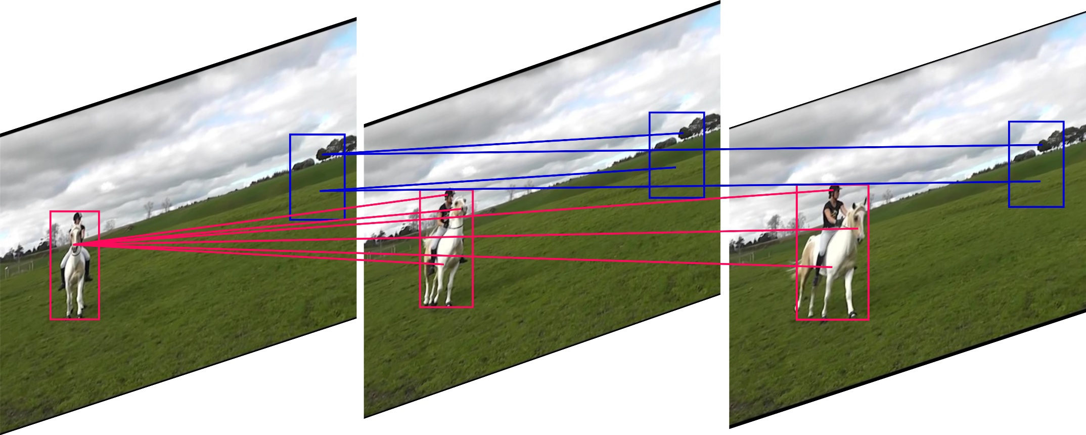
Figure 1: Illustration of static contexts (in blue) and motional contexts (in red) across neighbouring video frames. The human and horse are moving objects, while the grassland and sky are static background. Note that the static stuff is helpful for the recognition of moving objects, i.e., a human is riding a horse on the grassland.

As widely accepted, the contextual information plays a central role in image semantic segmentation [96, 36, 37, 93, 50, 103, 27, 16, 45, 5, 6, 7, 9, 90, 98, 88, 33, 107, 99]. When considering videos, the contextual information is twofold: static contexts and motional contexts, as shown in Fig. 1. The former refers to the contexts within the same video frame or the contexts of unchanged content across different frames. Image semantic segmentation has exploited such contexts (for images) a lot, mainly accounting for multi-scale [6, 7, 9, 88] and global/long-range information [98, 96, 33, 107]. Such information is essential not only for understanding the static scene but also for perceiving the holistic environment of videos. The latter, also known as temporal information, is responsible for better parsing moving object/stuff and capturing more effective scene representations with the help of motions. The motional context learning has been widely studied in video semantic segmentation [23, 60, 53, 35, 85, 54, 32, 69, 34, 4, 105, 47, 42], which usually relies on optical flows [19] to model motional contexts, ignoring the static contexts. Although each single aspect, i.e., static or motional contexts, has been well studied, how to learn static and motional contexts simultaneously deserves more attention, which is important for VSS.

Furthermore, static contexts and motional contexts are highly correlated, not isolated, because both contexts are complementary to each other to represent a video clip. Therefore, the ideal solution for VSS is to jointly learn static and motional contexts, i.e., generating a unified representation of static and motional contexts. A naïve solution is to apply recent popular self-attention [76, 18, 80] by taking feature vectors at all pixels in neighboring frames as tokens. This can directly model global relationships of all tokens, of course including both static and motional contexts. However, this naïve solution has some obvious drawbacks. For example, it is super inefficient due to the large number of tokens/pixels in a video clip, making this naïve solution unrealistic. It also contains too much redundant computation because most content in a video clip usually does not change much and it is unnecessary to compute attention for the repeated content. Moreover, the too long length of tokens would affect the performance of self-attention, as shown in [84, 56, 29, 21, 12] where the reduction of the token length through downsampling leads to better performance. More discussion about why traditional self-attention is inappropriate for video context learning can be found in §3.1.

In this paper, we propose a new Coarse-to-Fine Feature Mining (CFFM) technique, which consists of two parts: coarse-to-fine feature assembling and cross-frame feature mining. Specifically, we first apply a lightweight deep network [83] to extract features from each frame. Then, we assemble the extracted features from neighbouring frames in a coarse-to-fine manner. Here, we use a larger receptive field and a more coarse pooling if the frame is more distant from the target. This feature assembling operation has two meanings. On one hand, it organizes the features in a multi-scale way, and the farthest frame would have the largest receptive field and the most coarse pooling. Since the content in a few sequential frames usually does not change suddenly and most content may only have a little temporal inconsistency, this operation is expected to prepare data for learning static contexts. On the other hand, this feature assembling operation enables a large perception region for remote frames because the moving objects may appear in a large region for remote frames. This makes it suitable for learning motional contexts. At last, with the assembled features, we use the cross-frame feature mining technique to iteratively mine useful information from neighbouring frames for the target frame. This mining technique is a specially-designed non-self attention mechanism that has two different inputs, unlike commonly-used self-attention that only has one input [76, 18]. The output features enhanced by the CFFM can be directly used for the final prediction. We describe the technical motivations for CFFM in detail in §3.1.

The advantages of this new video context learning mechanism are four-fold. (1) The proposed CFFM technique can learn a unified representation of static contexts and motional contexts, both of which are of vital importance for VSS. (2) The CFFM technique can be added on top of frame feature extraction backbones to generate powerful video contextual features, with low complexity and limited computational cost. (3) Without bells and whistles, we achieve state-of-the-art results for VSS on standard benchmarks by using the CFFM module. (4) The CFFM technique has the potential to be extended to improve other video recognition tasks that need powerful video contexts.

2 Related Work

2.1 Image Semantic Segmentation

Image semantic segmentation has always been a key topic in the vision community, mainly because of its wide applications in real-world scenarios. Since the pioneer work of FCN [68] which adopts fully convolution networks to make densely pixel-wise predictions, a number of segmentation methods have been proposed with different motivations or techniques [94, 30, 104, 52, 78, 63, 61, 31, 10, 97, 81]. For example, some works try to design effective encoder-decoder network architectures to exploit multi-level features from different network layers [66, 62, 25, 1, 68, 9, 75, 51]. Some works impose extra boundary supervision to improve the prediction accuracy of details [89, 74, 99, 44, 77]. Some works utilize the attention mechanism to enhance the semantic representations [8, 46, 95, 22, 67, 101, 33, 107]. Besides these talent works, we want to emphasize that most research aims at learning powerful contextual information [5, 90, 96, 93, 50, 103, 17, 27, 99, 45, 37, 36], including multi-scale [6, 7, 9, 88, 27, 26, 45] and global/long-range information [98, 96, 33, 107]. The contextual information is also essential for VSS, but the video contexts are different from the image contexts, as discussed above.

2.2 Video Semantic Segmentation

Since the real world is dynamic rather than static, VSS is necessary for pushing semantic segmentation into more practical deployments. Previous research on VSS was limited by the available datasets [58]. Specifically, three datasets were available: Cityscapes [14], NYUDv2 [70], and CamVid [2]. They either only annotate several nonadjacent frames in a video clip or have a small scale, a low frame rate and low resolution. In fact, these datasets are usually used for image segmentation. Fortunately, the recent establishment of the VSPW dataset [58] which is large-scale and fully-annotated solves this problem.

Most of the existing VSS methods utilize the optical flow to capture temporal relations [23, 60, 53, 54, 69, 34, 105, 85, 42, 40, 57]. These methods usually adopt different smart strategies to balance the trade-off between accuracy and efficiency [40, 57]. Among them, some works aim at improving the segmentation accuracy by exploiting the temporal relations using the optical flow for feature warping [23, 53, 60] or the GAN-like architecture [24] for predictive feature learning [35]. The other works aim at improving the segmentation efficiency by using temporal consistency for feature propagation and reuse [34, 47, 69, 105], or directly reusing high-level features [69, 4], or adaptively selecting the key frame [85], or propagating segmentation results to neighbouring frames [42], or extracting features from different frames with different sub-networks [32], or considering the temporal consistency as extra training constraints [54]. Zhu et al. [106] utilized video prediction models to predict future frames as well as future segmentation labels, which are used as augmented data for training better image semantic segmentation models, not for VSS. Different from the above approaches, STT [43] and LMANet [65] directly models the interactions between the target and reference features to exploit the temporal information.

The above VSS approaches explore the temporal relation, here denoted as motional contexts. However, video contexts include two highly-correlated aspects: static and motional contexts. Those methods ignore the static contexts that are important for segmenting complicated scenes. This paper addresses this problem by proposing a new video context learning mechanism, capable of joint learning a unified representation of static and motional contexts.

2.3 Transformer

Vision transformer, a strong competitor of CNNs, has been widely adopted in various vision tasks [18, 56, 87, 49, 92, 55, 100, 91, 72], due to its powerful ability of modeling global connection within all the input tokens. Specifically, ViT [18] splits images into patches, constructs tokens and processes tokens using typical transformer layers. Swin [56] improves ViT by introducing shifted windows when computing self-attention and a hierarchical architecture. Focal [87] introduces both fine-grained and coarse-grained attention in architecture design. The effectiveness of transformers has been validated in segmentation [100, 83], tracking [11, 86], crowd counting [48, 72], multi-label classification [41] and so on. Despite the success of transformer in these tasks, the use of transformer layers in VSS is non-trivial due to the large number of tokens among video frames. Here, we propose a effective and efficient way to model the contextual information for VSS.

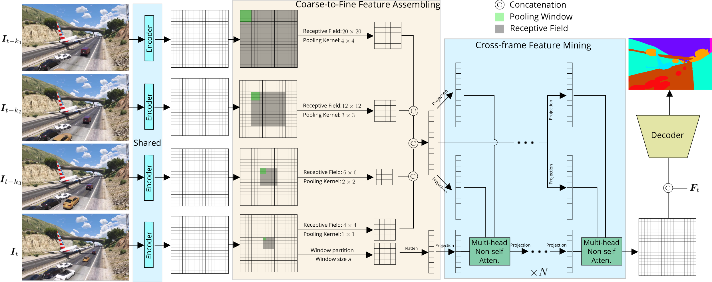
Figure 2: Overview of the proposed Coarse-to-Fine Feature Mining. All frames are first input to an encoder to extract features, which then go through the coarse-to-fine feature assembling module (CFFA). Features for different frames are processed by different pooling strategies to generate the context tokens. The principle is that for more distant frames, the bigger receptive field and more coarse pooling are used. The shown feature size ($20\times 20$), receptive field and pooling kernel are for simple explanation. The context tokens from all frames are concatenated and then processed by cross-frame feature mining (CFM) module. The context tokens are exploited to update the target features by several multi-head non-self attention layers. Finally, we use the enhanced target features to make segmentation prediction for the target frame. Best viewed with zooming.

3 Methodology

3.1 Technical Motivation

Before introducing our method, we discuss our technical motivation to help readers better understand the proposed technique. As discussed above, video contexts include static contexts and motional contexts. The former is well exploited in image semantic segmentation [96, 36, 37, 93, 50, 103, 15, 27, 26, 45, 5, 6, 7, 9, 90, 98, 88, 33, 107, 99], while the latter is studied in video semantic segmentation [47, 4, 23, 60, 53, 54, 69, 34, 105, 85, 42, 40, 57]. However, there is no research touching the joint learning of both static and motional contexts which are both essential for VSS.

To address this problem, a naïve solution is to simply apply the recently popular self-attention mechanism [76, 18, 80] to the video sequence by viewing the feature vector at each pixel of each frame as a token. In this way, we can model global relationships by connecting each pixel with all others, so all video contexts can of course be constructed. However, this naïve solution has three obvious drawbacks. First, a video sequence has $l$ times more tokens than a single image, where $l$ is the length of the video sequence. This would lead to $l^{2}$ times more computational cost than a single image because the complexity of the self-attention mechanism is $\mathcal{O}(N^{2}C)$, where $N$ is the number of tokens and $C$ is the feature dimension [76, 18, 56]. Such high complexity is unaffordable, especially for VSS that needs on-time processing as video data stream comes in sequence. Second, such direct global modeling would be redundant. Despite that there are some motions in a video clip, the overall semantics/environment would not change suddenly and most video content is repeated. Hence, most of connections built by the direct global modeling are unnecessary, i.e., self-to-self connections. Last but not least, although self-attention can technically model global relationships, a too long sequence length would limit its performance, as demonstrated in [79, 84, 56, 29, 21, 12] where downsampling features into small scales leads to better performance than the original long sequence length.

Instead of directly modeling global relationships, we propose to model relationships only among necessary tokens for the joint learning of static and motional contexts. Our CFFM technique consists of two steps. The first step, Coarse-to-Fine Feature Assembling (CFFA), assembles the features extracted from neighbouring frames in a temporally coarse-to-fine manner based on three observations. First, the moving objects/stuff can only move gradually across frames in practice, and the objects/stuff cannot move from one position to another far position suddenly. Thus, the region of the possible positions of (an) moving object/stuff in a frame gradually gets larger for farther frames. In other words, for one pixel in a frame, the farther the frames, the larger the correlated regions. Second, although some content may change across frames, the overall semantics and environment would not change much, which means that most video content may only have a little temporal inconsistency. Third, the little temporal inconsistency of the “static” content across neighbouring frames can be easily handled by the pooling operation which is scale- and rotation-invariant. Inspired by the second and third observations, a varied-size region sampling through the pooling operation in neighbouring frames can convey multi-scale contextual information. Therefore, the designed CFFA can perceive multi-scale contextual information (static contexts) and motional contexts. Specifically, each pixel in the target frame corresponds to a larger receptive field and a more coarse pooling in the farther frame, as depicted in Fig. 2. Note that the length of the sampled tokens is much shorter than that in the default self-attention.

The second step of CFFM, Cross-frame Feature Mining (CFM), is designed to mine useful information from the features of neighbouring frames. This is an attention-based process. However, unlike traditional self-attention [76, 18, 80] whose query, key, and value come from the same input, we propose to use a non-self attention mechanism, where the query is from the target frame and the key and value are from neighbouring frames. Besides, we only update the query during the iterative running of non-self attention, but we keep the context tokens unchanged. This is intuitive as our goal is to mine information from neighbouring frames and the update of context tokens is thus unnecessary. Compared with self-attention that needs to concatenate and process all assembled features, this non-self attention further reduces the computational cost.

3.2 Coarse-to-Fine Feature Assembling

Without loss of generalizability, we start our discussion on training data containing video frames $\{\bm{I}_{t-k_{1}},\cdots,\bm{I}_{t-k_{l}},\bm{I}_{t}\}$ with ground-truth segmentation of $\{\bm{S}_{t-k_{1}},\cdots,\bm{S}_{t-k_{l}},\bm{S}_{t}\}$, and we focus on segmenting $\bm{I}_{t}$. Specifically, $\bm{I}_{t}$ is the target frame and $\{\bm{I}_{t-k_{1}},\cdots,\bm{I}_{t-k_{l}}\}$ are $l$ previous frames which are $\{{k_{1}},\cdots,{k_{l}}\}$ frames away from $\bm{I}_{t}$, respectively. Let us denote $U=\{t-k_{1},\cdots,t-k_{l},t\}$ as the set of all frame subscripts. We first process $\{\bm{I}_{t-k_{1}},\cdots,\bm{I}_{t-k_{l}},\bm{I}_{t}\}$ using an encoder to extract informative features $\bm{F}=\{\bm{F}_{t-k_{1}},\cdots,\bm{F}_{t-k_{l}},\bm{F}_{t}\}$, each of which has the size of $\mathbb{R}^{h\times w\times c}$ ($h$, $w$, and $c$ represent height, width, and the number of channels, respectively). We aim to exploit $\bm{F}$ to generate better features for segmenting $\bm{I}_{t}$ as relevant and valuable video contexts exist in previous frames.

To efficiently establish long-range interactions between the reference frame features ($\{\bm{F}_{t-k_{1}},\cdots,\bm{F}_{t-k_{l}}\}$) and the target frame features $\bm{F}_{t}$, we propose the coarse-to-fine feature assembling module, as showed in Fig. 2. Inspired by previous works [56, 79, 87], we split the target frame features $\bm{F}_{t}$ into windows and each window attends to a shared set of context tokens. The reason behind this is that attending each location in $\bm{F}_{t}$ to a specific set of context tokens requires huge computation and memory cost. When using window size of $s\times s$, $\bm{F}_{t}$ is partitioned into $\frac{h}{s}\times\frac{w}{s}$ windows. We obtain the new feature map $\bm{F}^{{}^{\prime}}_{t}$ as follows:

$$\bm{F}_{t}\in\mathbb{R}^{h\times w\times c} \to\bm{F}^{\prime}_{t}\in\mathbb{R}^{(\frac{h}{s}\times s)\times(\frac{w}{s}\times s)\times c}\to\bm{F}^{\prime}_{t}\in\mathbb{R}^{\frac{h}{s}\times\frac{w}{s}\times s\times s\times c}.$$ (1)

Then, we generate context tokens from different frames. The main idea is to see a bigger receptive field and use a more coarse pooling if the frame is more distant from the target, which is why we call this step coarse-to-fine feature assembling. The motivation behind this is described in §3.1. Formally, we define two sets of parameters: the receptive fields $r=\{r_{t-k_{1}},\cdots,r_{t-k_{l}},r_{t}\}$ and the pooling kernel/window sizes $p=\{p_{t-k_{1}},\cdots,p_{t-k_{l}},p_{t}\}$, when generating corresponding context tokens. For $t-k_{1}<t-k_{2}<\cdots<t-k_{l}<t$, we have $r_{t-k_{1}}\geq r_{t-k_{2}}\geq\cdots\geq r_{t-k_{l}}\geq r_{t}$ and $p_{t-k_{1}}\geq p_{t-k_{2}}\geq\cdots\geq p_{t-k_{l}}\geq p_{t}$. With this definition, we partition $\{\bm{F}_{t-k_{1}},\cdots,\bm{F}_{t-k_{l}},\bm{F}_{t}\}$ using pooling windows $p=\{p_{t-k_{1}},\cdots,p_{t-k_{l}},p_{t}\}$ to pool the features, respectively. The result is processed by a fully connected layer (FC) for dimension reduction. This is formulated as

$$\bm{F}_{j}\in\mathbb{R}^{h\times w\times c} \to\bm{E}_{j}\in\mathbb{R}^{\frac{h}{p_{j}}\times\frac{w}{p_{j}}\times c\times p_{j}^{2}}\stackrel{{\scriptstyle\rm FC}}{{\to}}\bm{E}_{j}\in\mathbb{R}^{\frac{h}{p_{j}}\times\frac{w}{p_{j}}\times c},$$ (2)

where $j\in U$. In Fig. 2, we have $r=\{20,12,6,4\}$ and $p=\{4,3,2,1\}$ for all frames (3 reference and 1 target).

For each window partition $\bm{F}^{\prime}_{t}[i]\in\mathbb{R}^{s\times s\times c}$ ($i\in\{1,2,\cdots,\frac{hw}{s^{2}}\}$) in the target features, we extract $\frac{r_{j}}{p_{j}}\times\frac{r_{j}}{p_{j}}$ elements from $\bm{E}_{j}$ around the area where the window lies in. This can be easily implemented using the unfold function in PyTorch [64]. Let $\bm{c}_{i,j}$ denote the obtained context tokens from $j$-th frame and for $i$-th window partition in the target features. We concatenate $\bm{c}_{i,j}$ into $\bm{c}_{i}$ as follows,

$$\footnotesize\bm{c}_{i}={\rm Concat}[\bm{c}_{i,j}],$$ (3)

where $j\in U$, $\bm{c}_{i}\in\mathbb{R}^{m\times c}$ and $m=\sum_{j\in U}\frac{r^{2}_{j}}{p^{2}_{j}}$. The context tokens from the target frame are obtained by using parameter set ($r_{t}$, $p_{t}$) to process the target features. In practice, we additionally use another parameter set ($r_{t}^{{}^{\prime}}$, $p_{t}^{{}^{\prime}}$) to generate more contexts from the target since the target features are more important. For simplicity, we focus our discussion by omitting ($r_{t}^{{}^{\prime}}$, $p_{t}^{{}^{\prime}}$) and using only ($r_{t}$, $p_{t}$) for the target.

To sum up, $\bm{c}_{i}$ contains the context information from all frames, which is used to refine the target frame features. As discussed in §3.1, on one hand, $\bm{c}_{i}$ covers the tokens at possible positions that moving objects/stuff would appear, so it can be used for learning motional contexts. On the other hand, $\bm{c}_{i}$ is a multi-scale sampling of neighbouring frames with the temporal inconsistency solved by the pooling operation, so it can be used for learning static contexts.

3.3 Cross-frame Feature Mining

After that we obtain the context tokens $\bm{c}_{i}$, for each window partition in the target features, we propose a non-self attention mechanism to mine useful information from neighboring frames. Unlike the traditional self-attention mechanism that computes the query, key, and value from the same input, our non-self attention mechanism utilizes different inputs to calculate the query, key, and value. Since $\bm{F}^{{}^{\prime}}_{t}$ is the input to the first layer of our cross-frame feature mining module, we re-write it as $\bm{F}^{0}_{t}=\bm{F}^{{}^{\prime}}_{t}$. For the $i$-th window partition in $\bm{F}^{0}_{t}$, the query $Q_{i}$, key $K_{i}$, and value $V_{i}$ are computed using three fully connected layers as follows:

$$\footnotesize\begin{split}Q_{i}={\rm FC}(\bm{F}^{0}_{t}[i]),~{}~{}~{}K_{i}={\rm FC}(\bm{c}_{i}),~{}~{}~{}V_{i}={\rm FC}(\bm{c}_{i}),\end{split}$$ (4)

where ${\rm FC}(\cdot)$ represents a FC layer. Next, we use non-self attention to update the target frame features, given by

$$\footnotesize\begin{split}\bm{F}^{1}_{t}[i]=\text{Softmax}(\frac{Q_{i}K_{i}^{T}}{\sqrt{c}}+B)V_{i}+\bm{F}^{0}_{t}[i],\end{split}$$ (5)

where $B$ represents the position bias, following [56]. Note that we omit the formulation of the multi-head attention [76, 18] for simplicity. Equ. (4) and Equ. (5) are repeated for $N$ steps, and we finally obtain the enhanced feature $\bm{F}^{N}_{t}\in\mathbb{R}^{\frac{h}{s}\times\frac{w}{s}\times s\times s\times c}$ for the target frame. Long-range static and motional contexts from neighbouring frames are continuously exploited to learn better features for segmenting the target frame. Note that in this process, we do not update the context tokens $\bm{c}_{i}$ for simplicity/elegance and reducing computation. Since this step is to mine useful information from the reference frames, it is also unnecessary to update $\bm{c}_{i}$. This is the advantage of non-self attention.

To generate segmentation predictions, we reshape $\bm{F}^{N}_{t}$ into $\mathbb{R}^{h\times w\times c}$ and concatenate $\bm{F}^{N}_{t}$ with $\bm{F}_{t}$. Then, a simple MLP projects the features to segmentation logits. The common cross entropy (CE) is used as the loss function for training. Auxiliary losses on original features are also computed. During inference, our method does not need to extract features for all $l+1$ frames when processing $\bm{I}_{t}$. Instead, the features of the reference frames, which are the frames before the target frame, have already been extracted in previous steps. Only the target frame is passed to the encoder to generate $\bm{F}_{t}$, and then features $\{\bm{F}_{t-k_{1}},\cdots,\bm{F}_{t-k_{l}},\bm{F}_{t}\}$ for all frames are passed to the CFFM.

3.4 Complexity Analysis

Here, we formally analyze the complexity of the proposed CFFM and the recent popular self-attention mechanism [76, 18, 80] when processing video clip features $\{\bm{F}_{t-k_{1}},\cdots,\bm{F}_{t-k_{l}},\bm{F}_{t}\}$. The coarse-to-fine feature assembling (Equ. (2)) has the complexity of $\mathcal{O}((l+1)hwc)$, which is irrespective of $p$. The cross-frame feature mining has two parts: Equ. (4) has the complexity of $\mathcal{O}(hwc^{2})+\mathcal{O}(mc^{2})$, and Equ. (5) is with the complexity of $\mathcal{O}(hwmc)$. As mentioned early, $m=\sum_{j\in U}\frac{r^{2}_{j}}{p^{2}_{j}}$. To sum over, the complexity of our method is given by

$$\scriptsize\begin{split}\mathcal{O}({\rm CFFM})&=\mathcal{O}(hwmc)+\mathcal{O}(hwc^{2})+\mathcal{O}(mc^{2})+\mathcal{O}((l+1)hwc)\\ &=\mathcal{O}(hwmc)+\mathcal{O}(hwc^{2}),\end{split}$$ (6)

where the derivation is conducted by removing less significant terms. For the self-attention mechanism [76, 18, 80], the complexity is $\mathcal{O}((l+1)^{2}h^{2}w^{2}c)+\mathcal{O}((l+1)hwc^{2})$. Since $m\ll(l+1)^{2}hw$, the complexity of the proposed approach is much less than the self-attention mechanism. Take the example in Fig. 2, $m=66$ while $(l+1)^{2}hw=6400$.

3.5 Difference with STT

We notice that a concurrent work STT [43] also utilizes bigger searching regions for more distant frames and self-attention mechanisms to establish connections across frames. While two works share these similarities, there are key differences between them. First, two methods have different motivations. We target at exploiting both static and motional contexts, while STT focuses on capturing the temporal relations among complex regions. Note that the concept of static/motional contexts is similar to the concept of simple/complex regions in STT. As a result, STT models only the motional contexts, while our method models both static and motional contexts. Second, the designs are different. For query selection, STT selects 50% of query locations in order to reduce the computation. However, our method splits the query features into windows and the query features in each window share the same contexts to reduce the computation. For key/value selection, STT operates in the same granularity, while our method processes the selected key/value into different granularity, which reduces the number of tokens and models the multi-scale information for static contexts. Third, our cross-frame feature mining can exploit multiple transformer layers to deeply mine the contextual information from the reference frames, but STT only uses one layer. The reason may be that STT only updates the query features of the selected locations and using multiple STT layers could lead to inconsistency in the query features in un-selected and selected locations.

4 Experiments

4.1 Experimental Setup

Implementation details. We implement our approach based on the $mmsegmentation$ [13] codebase and conduct all experiments on 4 NVIDIA GPUs. The backbones are the same as SegFormer [83], which are all pretrained on ImageNet [39]. For other parts of our model, we adopt random initialization. Our model uses 3 reference frames unless otherwise specified, and $\{k_{1},k_{2},k_{3}\}=\{9,6,3\}$, following [58]. We found that this selection of reference frames is enough to include rich context and achieve impressive performance. For the receptive field, pooling kernel and window size, we set $r=\{49,20,6,7\}$, $p=\{7,4,2,1\}$ and $s=7$. For the target frame, we additionally have $r_{t}^{{}^{\prime}}=35$ and $p_{t}^{{}^{\prime}}=5$. During training, we adopt augmentations including random resizing, flipping, cropping, and photometric distortion. We use the crop size of $480\times 480$ for the VSPW dataset [58] and $512\times 1024$ for Cityscapes [14]. For optimizing parameters, we use the AdamW and “poly” learning rate schedule, with an initial learning rate of 6$e$-5. During testing, we conduct single-scale test and resize all images on VSPW to the size of $480\times 853$ and $512\times 1024$ for Cityscapes. Note that for efficiency and simplicity, the predicted mask is obtained by feeding the whole image to the network, rather than using sliding window as in [100]. We do not use any post-processing such as CRF [38].

Datasets.  Our experiments are mainly conducted on the VSPW dataset [58], which is the largest video semantic segmentation benchmark. Its training, validation and test sets have 2,806 clips (198,244 frames), 343 clips (24,502 frames), and 387 clips (28,887 frames), respectively. It contains diverse scenarios including both indoor and outdoor scenes, annotated for 124 categories. More importantly, VSPW has dense annotations with a high frame rate of 15fps, making itself the best benchmark for video semantic segmentation till now. In contrast, previous datasets used for video semantic segmentation only have very sparse annotation, i.e., only one frame out of many consecutive frames is annotated. In addition, we also evaluate the proposed method on the Cityscapes dataset [14], which annotates one frame out of every 30 frames.

Evaluation metrics.  Following previous works [68], we use mean IoU (mIoU), and weigheted IoU to evaluate the segmentation performance. In addition, we also adopt video consistency (VC) [58] to evaluate the smoothness of the predicted segmentation maps across the temporal domain. Formally, for a video clips $\{\bm{I}_{c}\}_{c=1}^{C}$ with ground truth masks $\{\bm{S}_{c}\}_{c=1}^{C}$ and predicted masks $\{\bm{S}^{{}^{\prime}}_{c}\}_{c=1}^{C}$, VC_n is computed as follows,

$$\footnotesize\begin{split}\text{VC}_{n}=\frac{1}{C-n+1}\sum_{i=1}^{C-n+1}\frac{(\cap_{i}^{i+n-1}\bm{S}_{i})\cap(\cap_{i}^{i+n-1}\bm{S}^{{}^{\prime}}_{i})}{\cap_{i}^{i+n-1}\bm{S}_{i}},\end{split}$$ (7)

where $C\geq n$. After computing VC_n for every video, we obtain the mean of VC_n for all videos as mVC_n. The purpose of this metric is to evaluate the level of consistency in the predicted masks among those common areas (pixels’ semantic labels don’t change) across long-range frames. For more details, please refer to [58]. Note that to compute VC metric, the ground-truth masks for all frames are needed.

Methods	Backbone	Params (M) $\downarrow$	mIoU $\uparrow$	Weighted IoU $\uparrow$	mVC8 $\uparrow$	mVC16 $\uparrow$	FPS (f/s) $\uparrow$
SegFormer [83]	MiT-B0	3.8	32.9	56.8	82.7	77.3	73.4
SegFormer [83]	MiT-B1	13.8	36.5	58.8	84.7	79.9	58.7
CFFM (Ours)	MiT-B0	4.7	35.4	58.5	87.7	82.9	43.1
CFFM (Ours)	MiT-B1	15.5	38.5	60.0	88.6	84.1	29.8
DeepLabv3+ [7]	ResNet-101	62.7	34.7	58.8	83.2	78.2	-
UperNet [82]	ResNet-101	83.2	36.5	58.6	82.6	76.1	-
PSPNet [98]	ResNet-101	70.5	36.5	58.1	84.2	79.6	13.9
OCRNet [93]	ResNet-101	58.1	36.7	59.2	84.0	79.0	14.3
ETC [54]	PSPNet	89.4	36.6	58.3	84.1	79.2	-
NetWarp [82]	PSPNet	89.4	37.0	57.9	84.4	79.4	-
ETC [54]	OCRNet	58.1	37.5	59.1	84.1	79.1	-
NetWarp [82]	OCRNet	58.1	37.5	58.9	84.0	79.0	-
TCB${}_{\text{st-ppm}}$ [58]	ResNet-101	70.5	37.5	58.6	87.0	82.1	10.0
TCB${}_{\text{st-ocr}}$ [58]	ResNet-101	58.1	37.4	59.3	86.9	82.0	5.5
TCB${}_{\text{st-ocr-mem}}$ [58]	ResNet-101	58.1	37.8	59.5	87.9	84.0	5.5
SegFormer [83]	MiT-B2	24.8	43.9	63.7	86.0	81.2	39.2
SegFormer [83]	MiT-B5	82.1	48.2	65.1	87.8	83.7	17.2
CFFM (Ours)	MiT-B2	26.5	44.9	64.9	89.8	85.8	23.8
CFFM (Ours)	MiT-B5	85.5	49.3	65.8	90.8	87.1	11.3

Table 1: Comparison with state-of-the-art methods on the VSPW [58] validation set. Our model outperforms the compared methods, with better balance in terms of model size, performance and speed.

4.2 Comparison with State-of-the-art Methods

We compare the proposed method with state-of-the-art algorithms on VSPW [58] in Tab. 1. The results are analyzed from different aspects. For small models (# of parameters $<$ 20M), our method outperforms corresponding baseline with a clear margin, while introducing limited model complexity. For example, using the backbone MiT-B0, we obtain 2.5% mIoU gain over the strong baseline of SegFormer [83], with the cost of increasing the parameters from 13.8M to 15.5M and reducing the FPS from 73.4 to 43.1. Our method also provides much more consistent predictions for the videos, outperforming the baseline with 5.0% and 5.6% in mVC₈ and mVC₁₆, respectively.

For large models, our approach achieves the new state-of-the-art performance in this challenging dataset and also generates visually consistent results. Specifically, our model with 26.5M parameters (slightly larger than SegFormer [83] with MiT-B2) achieves 44.9% mIoU at the frame rate of 23.8fps. Our large model (based on MiT-B5) achieves mIoU of 49.3% and performs best in terms of visual consistency, with mVC₈ and mVC₁₆ of 90.8% and 87.1%, respectively. For all backbones (MiT-B0, MiT-B1, MiT-B2 and MiT-B5), CFFM clearly outperforms the corresponding baselines, showing that the proposed modules are stable. The results validate the effectiveness of the proposed coarse-to-fine feature assembling and cross-frame feature mining in mining informative contexts from all frames.

For Cityscapes [14] dataset, our method is compared with recent efficient segmentation methods. Only using 4.6M parameters, our model obtains 74.0% mIoU with frame rate of 34.2fps, achieving an excellent balance on model size, performance and speed. When using deeper backbone, we achieve 75.1% mIoU with the frame rate of 23.6fps. Note that this dataset has sparse annotations, the excellent performance demonstrates that our method works well for both fully supervised and semi-supervised settings.

The qualitative results are shown in Fig. 3. For the given example, our method resolves the inconsistency existing in the predictions of the baseline, due to the use of rich contextual information from the all frames.

Methods	Backbone	Params (M)	mIoU	FPS (f/s)
FCN [68]	MobileNetV2	9.8	61.5	14.2
CC [69]	VGG-16	-	67.7	16.5
DFF [105]	ResNet-101	-	68.7	9.7
GRFP [60]	ResNet-101	-	69.4	3.2
PSPNet [98]	MobileNetV2	13.7	70.2	11.2
DVSN [85]	ResNet-101	-	70.3	19.8
Accel [34]	ResNet-101	-	72.1	3.6
ETC [54]	ResNet-18	13.2	71.1	9.5
SegFormer [83]	MiT-B0	3.7	71.9	58.5
CFFM (Ours)	MiT-B0	4.6	74.0	34.2
SegFormer [83]	MiT-B1	13.8	74.1	46.8
CFFM (Ours)	MiT-B1	15.4	75.1	23.6

Table 2: Comparison with recent efficient video semantic segmentation methods on the Cityscapes [14] dataset.

Figure 3: Qualitative results. We compare the proposed method with the baseline (SegFormer [83]) visually. From top to down: the input video frames, the predictions of SegFormer [83], our predictions, and the ground truth. It shows that our model produces more accurate and consistent results, compared to the strong baseline. Best viewed in color.

Methods	Backbone	$N$	mIoU	mVC8	mVC16	Params (M)
SegFormer [83]	MiT-B0	-	32.9	82.7	77.3	3.8
CFFM (Ours)	MiT-B0	1	35.4	87.7	82.9	4.7
	MiT-B0	2	35.7	87.7	83.0	5.5
SegFormer [83]	MiT-B1	-	36.5	84.7	79.9	13.8
CFFM (Ours)	MiT-B1	1	37.8	88.3	83.6	14.6
	MiT-B1	2	38.5	88.6	84.1	15.5
	MiT-B1	3	38.7	88.6	84.1	16.3
	MiT-B1	4	38.8	88.5	83.9	17.2

Table 3: Ablation study on the number of attention layers in cross-frame feature mining module.

Methods	k1	k2	k3	mIoU	mVC8	mVC16
SegFormer	-	-	-	36.5	84.7	79.9
CFFM (Ours)	-	-	3	37.4	87.4	82.4
	-	-	6	37.7	88.0	83.3
	-	-	9	37.9	88.4	83.9
	3	2	1	37.7	88.3	83.6
	9	6	3	38.5	88.6	84.1

Table 4: Ablation study on the selection of the reference frames. We use MiT-B1 as the backbone.

4.3 Ablation Study

All ablation studies are conducted on the large-scale VSPW [58] dataset and follows the same training strategies as described above, for fair comparison.

Influence of the number of attention layers.  Tab. 3 shows the performance of our method with respect to the number of non-self attention layers in cross-frame feature mining module. For two backbones of MiT-B0 [83] and MiT-B1 [83], our method clearly outperforms the corresponding baseline (SegFormer) when only using a single attention layer and introducing a small amount of additional parameters. It demonstrates the effectiveness of the proposed coarse-to-fine feature assembling module and the attention layer. The former efficiently extracts the context information from the frames and the latter effectively mine the information to refine target features. In addition, we observe there is a trade-off between performance and the model complexity on MiT-B1 backbone. When using more attention layers, better mIoU is obtained while the model size linearly increases. For our method on MiT-B1, we choose $N=2$ since better trade-off is obtained.

Impact of selection of reference frames.  We study the impact of the selection of reference frames in Tab. 4. We start by using a single reference frame. There seems to be a trend that when increasing the distance between the reference frame and the target frame, better performance is obtained. The possible reason for this is that the far-away reference frame may contain richer and different context which complements the one of the target frame. When using more reference frames ($k_{1}=9,k_{2}=6,k_{3}=3$), the best performance is achieved. It is worthy noting that the reference frames combination of $k_{1}=3,k_{2}=2$, and $k_{3}=1$, performs similarly as the cases when using single reference frame, possibly due to the fact that the close reference frames don’t give much new information for segmenting the target frame.

Impact of CFFA and CFM  Starting from SegFormer [83], we first add CFFA by using MLP to process the context tokens and then merge them with the target features. We obtain mIoU of 37.6. Then we add both CFFA and CFM on the baseline, which is our final model. The segmentation mIoU is 38.5. It shows that both CFFA and CFM are valuable for the proposed CFFM mechanism.

5 Conclusion

The video contexts include static contexts and motional contexts, both of which are essential for video semantic segmentation. Previous methods pay much attention to motional contexts but ignore the static contexts. To this end, this paper proposes a Coarse-to-Fine Feature Mining (CFFM) technique to jointly learn a unified presentation of static and motional contexts, for precise and efficient VSS. CFFM contains two parts: coarse-to-fine feature assembling and cross-frame feature mining. The former summarizes contextual information with different granularity for different frames, according to their distance to the target frame. The latter efficiently mines the contexts from neighbouring frames to enhance the feature of the target frame. While adding limited computational resources, CFFM boosts segmentation performance in a clear margin.

References

- [1] Vijay Badrinarayanan, Alex Kendall, and Roberto Cipolla. SegNet: A deep convolutional encoder-decoder architecture for image segmentation. IEEE TPAMI, 39(12):2481–2495, 2017.
- [2] Gabriel J. Brostow, Jamie Shotton, Julien Fauqueur, and Roberto Cipolla. Segmentation and recognition using structure from motion point clouds. In ECCV, pages 44–57, 2008.
- [3] Holger Caesar, Jasper Uijlings, and Vittorio Ferrari. COCO-Stuff: Thing and stuff classes in context. In IEEE CVPR, pages 1209–1218, 2018.
- [4] Joao Carreira, Viorica Patraucean, Laurent Mazare, Andrew Zisserman, and Simon Osindero. Massively parallel video networks. In ECCV, pages 649–666, 2018.
- [5] Liang-Chieh Chen, George Papandreou, Iasonas Kokkinos, Kevin Murphy, and Alan L Yuille. Semantic image segmentation with deep convolutional nets and fully connected CRFs. In ICLR, 2015.
- [6] Liang-Chieh Chen, George Papandreou, Iasonas Kokkinos, Kevin Murphy, and Alan L Yuille. DeepLab: Semantic image segmentation with deep convolutional nets, atrous convolution, and fully connected CRFs. IEEE TPAMI, 40(4):834–848, 2018.
- [7] Liang-Chieh Chen, George Papandreou, Florian Schroff, and Hartwig Adam. Rethinking atrous convolution for semantic image segmentation. arXiv preprint arXiv:1706.05587, 2017.
- [8] Liang-Chieh Chen, Yi Yang, Jiang Wang, Wei Xu, and Alan L Yuille. Attention to scale: Scale-aware semantic image segmentation. In IEEE CVPR, pages 3640–3649, 2016.
- [9] Liang-Chieh Chen, Yukun Zhu, George Papandreou, Florian Schroff, and Hartwig Adam. Encoder-decoder with atrous separable convolution for semantic image segmentation. In ECCV, pages 801–818, 2018.
- [10] Wanli Chen, Xinge Zhu, Ruoqi Sun, Junjun He, Ruiyu Li, Xiaoyong Shen, and Bei Yu. Tensor low-rank reconstruction for semantic segmentation. In ECCV, pages 52–69, 2020.
- [11] Xin Chen, Bin Yan, Jiawen Zhu, Dong Wang, Xiaoyun Yang, and Huchuan Lu. Transformer tracking. In IEEE CVPR, pages 8126–8135, 2021.
- [12] Xiangxiang Chu, Zhi Tian, Yuqing Wang, Bo Zhang, Haibing Ren, Xiaolin Wei, Huaxia Xia, and Chunhua Shen. Twins: Revisiting the design of spatial attention in vision transformers. In NeurIPS, 2021.
- [13] MMSegmentation Contributors. MMSegmentation: Openmmlab semantic segmentation toolbox and benchmark. https://github.com/open-mmlab/mmsegmentation, 2020.
- [14] Marius Cordts, Mohamed Omran, Sebastian Ramos, Timo Rehfeld, Markus Enzweiler, Rodrigo Benenson, Uwe Franke, Stefan Roth, and Bernt Schiele. The Cityscapes dataset for semantic urban scene understanding. In IEEE CVPR, pages 3213–3223, 2016.
- [15] Henghui Ding, Xudong Jiang, Ai Qun Liu, Nadia Magnenat Thalmann, and Gang Wang. Boundary-aware feature propagation for scene segmentation. In IEEE ICCV, pages 6819–6829, 2019.
- [16] Henghui Ding, Xudong Jiang, Bing Shuai, Ai Qun Liu, and Gang Wang. Context contrasted feature and gated multi-scale aggregation for scene segmentation. In IEEE CVPR, pages 2393–2402, 2018.
- [17] Henghui Ding, Xudong Jiang, Bing Shuai, Ai Qun Liu, and Gang Wang. Semantic correlation promoted shape-variant context for segmentation. In IEEE CVPR, pages 8885–8894, 2019.
- [18] Alexey Dosovitskiy, Lucas Beyer, Alexander Kolesnikov, Dirk Weissenborn, Xiaohua Zhai, Thomas Unterthiner, Mostafa Dehghani, Matthias Minderer, Georg Heigold, Sylvain Gelly, Jakob Uszkoreit, and Neil Houlsby. An image is worth 16x16 words: Transformers for image recognition at scale. In ICLR, 2021.
- [19] Alexey Dosovitskiy, Philipp Fischer, Eddy Ilg, Philip Hausser, Caner Hazirbas, Vladimir Golkov, Patrick Van Der Smagt, Daniel Cremers, and Thomas Brox. FlowNet: Learning optical flow with convolutional networks. In IEEE ICCV, pages 2758–2766, 2015.
- [20] Mark Everingham, SM Ali Eslami, Luc Van Gool, Christopher KI Williams, John Winn, and Andrew Zisserman. The pascal visual object classes challenge: A retrospective. IJCV, 111(1):98–136, 2015.
- [21] Haoqi Fan, Bo Xiong, Karttikeya Mangalam, Yanghao Li, Zhicheng Yan, Jitendra Malik, and Christoph Feichtenhofer. Multiscale vision transformers. In IEEE ICCV, pages 6824–6835, 2021.
- [22] Jun Fu, Jing Liu, Haijie Tian, Yong Li, Yongjun Bao, Zhiwei Fang, and Hanqing Lu. Dual attention network for scene segmentation. In IEEE CVPR, pages 3146–3154, 2019.
- [23] Raghudeep Gadde, Varun Jampani, and Peter V Gehler. Semantic video CNNs through representation warping. In IEEE ICCV, pages 4453–4462, 2017.
- [24] Ian Goodfellow, Jean Pouget-Abadie, Mehdi Mirza, Bing Xu, David Warde-Farley, Sherjil Ozair, Aaron Courville, and Yoshua Bengio. Generative adversarial nets. In NeurIPS, 2014.
- [25] Bharath Hariharan, Pablo Arbeláez, Ross Girshick, and Jitendra Malik. Hypercolumns for object segmentation and fine-grained localization. In IEEE CVPR, pages 447–456, 2015.
- [26] Junjun He, Zhongying Deng, and Yu Qiao. Dynamic multi-scale filters for semantic segmentation. In IEEE ICCV, pages 3562–3572, 2019.
- [27] Junjun He, Zhongying Deng, Lei Zhou, Yali Wang, and Yu Qiao. Adaptive pyramid context network for semantic segmentation. In IEEE CVPR, pages 7519–7528, 2019.
- [28] Kaiming He, Xiangyu Zhang, Shaoqing Ren, and Jian Sun. Deep residual learning for image recognition. In IEEE CVPR, pages 770–778, 2016.
- [29] Byeongho Heo, Sangdoo Yun, Dongyoon Han, Sanghyuk Chun, Junsuk Choe, and Seong Joon Oh. Rethinking spatial dimensions of vision transformers. In IEEE ICCV, pages 11936–11945, 2021.
- [30] Chi-Wei Hsiao, Cheng Sun, Hwann-Tzong Chen, and Min Sun. Specialize and fuse: Pyramidal output representation for semantic segmentation. In IEEE ICCV, pages 7137–7146, 2021.
- [31] Hanzhe Hu, Deyi Ji, Weihao Gan, Shuai Bai, Wei Wu, and Junjie Yan. Class-wise dynamic graph convolution for semantic segmentation. In ECCV, pages 1–17, 2020.
- [32] Ping Hu, Fabian Caba, Oliver Wang, Zhe Lin, Stan Sclaroff, and Federico Perazzi. Temporally distributed networks for fast video semantic segmentation. In IEEE CVPR, pages 8818–8827, 2020.
- [33] Zilong Huang, Xinggang Wang, Lichao Huang, Chang Huang, Yunchao Wei, and Wenyu Liu. CCNet: Criss-cross attention for semantic segmentation. In IEEE ICCV, pages 603–612, 2019.
- [34] Samvit Jain, Xin Wang, and Joseph E Gonzalez. Accel: A corrective fusion network for efficient semantic segmentation on video. In IEEE CVPR, pages 8866–8875, 2019.
- [35] Xiaojie Jin, Xin Li, Huaxin Xiao, Xiaohui Shen, Zhe Lin, Jimei Yang, Yunpeng Chen, Jian Dong, Luoqi Liu, Zequn Jie, et al. Video scene parsing with predictive feature learning. In IEEE ICCV, pages 5580–5588, 2017.
- [36] Zhenchao Jin, Tao Gong, Dongdong Yu, Qi Chu, Jian Wang, Changhu Wang, and Jie Shao. Mining contextual information beyond image for semantic segmentation. In IEEE ICCV, pages 7231–7241, 2021.
- [37] Zhenchao Jin, Bin Liu, Qi Chu, and Nenghai Yu. ISNet: Integrate image-level and semantic-level context for semantic segmentation. In IEEE ICCV, pages 7189–7198, 2021.
- [38] Philipp Krähenbühl and Vladlen Koltun. Efficient inference in fully connected CRFs with Gaussian edge potentials. In NeurIPS, pages 109–117, 2011.
- [39] Alex Krizhevsky, Ilya Sutskever, and Geoffrey E Hinton. ImageNet classification with deep convolutional neural networks. In NeurIPS, volume 25, pages 1097–1105, 2012.
- [40] Abhijit Kundu, Vibhav Vineet, and Vladlen Koltun. Feature space optimization for semantic video segmentation. In IEEE CVPR, pages 3168–3175, 2016.
- [41] Jack Lanchantin, Tianlu Wang, Vicente Ordonez, and Yanjun Qi. General multi-label image classification with transformers. In IEEE CVPR, pages 16478–16488, 2021.
- [42] Shih-Po Lee, Si-Cun Chen, and Wen-Hsiao Peng. GSVNet: Guided spatially-varying convolution for fast semantic segmentation on video. In IEEE ICME, pages 1–6, 2021.
- [43] Jiangtong Li, Wentao Wang, Junjie Chen, Li Niu, Jianlou Si, Chen Qian, and Liqing Zhang. Video semantic segmentation via sparse temporal transformer. In ACM MM, pages 59–68, 2021.
- [44] Xiangtai Li, Xia Li, Li Zhang, Guangliang Cheng, Jianping Shi, Zhouchen Lin, Shaohua Tan, and Yunhai Tong. Improving semantic segmentation via decoupled body and edge supervision. In ECCV, pages 435–452, 2020.
- [45] Xia Li, Yibo Yang, Qijie Zhao, Tiancheng Shen, Zhouchen Lin, and Hong Liu. Spatial pyramid based graph reasoning for semantic segmentation. In IEEE CVPR, pages 8950–8959, 2020.
- [46] Xia Li, Zhisheng Zhong, Jianlong Wu, Yibo Yang, Zhouchen Lin, and Hong Liu. Expectation-maximization attention networks for semantic segmentation. In IEEE ICCV, pages 9167–9176, 2019.
- [47] Yule Li, Jianping Shi, and Dahua Lin. Low-latency video semantic segmentation. In IEEE CVPR, pages 5997–6005, 2018.
- [48] Dingkang Liang, Xiwu Chen, Wei Xu, Yu Zhou, and Xiang Bai. Transcrowd: Weakly-supervised crowd counting with transformer. arXiv preprint arXiv:2104.09116, 2021.
- [49] Jingyun Liang, Jiezhang Cao, Guolei Sun, Kai Zhang, Luc Van Gool, and Radu Timofte. Swinir: Image restoration using swin transformer. In IEEE ICCV, pages 1833–1844, 2021.
- [50] Jianbo Liu, Junjun He, Yu Qiao, Jimmy S Ren, and Hongsheng Li. Learning to predict context-adaptive convolution for semantic segmentation. In ECCV, pages 769–786, 2020.
- [51] Jianbo Liu, Junjun He, Jiawei Zhang, Jimmy S Ren, and Hongsheng Li. EfficientFCN: Holistically-guided decoding for semantic segmentation. In ECCV, pages 1–17, 2020.
- [52] Mingyuan Liu, Dan Schonfeld, and Wei Tang. Exploit visual dependency relations for semantic segmentation. In IEEE CVPR, pages 9726–9735, 2021.
- [53] Si Liu, Changhu Wang, Ruihe Qian, Han Yu, Renda Bao, and Yao Sun. Surveillance video parsing with single frame supervision. In IEEE CVPR, pages 413–421, 2017.
- [54] Yifan Liu, Chunhua Shen, Changqian Yu, and Jingdong Wang. Efficient semantic video segmentation with per-frame inference. In ECCV, pages 352–368, 2020.
- [55] Yun Liu, Guolei Sun, Yu Qiu, Le Zhang, Ajad Chhatkuli, and Luc Van Gool. Transformer in convolutional neural networks. arXiv preprint arXiv:2106.03180, 2021.
- [56] Ze Liu, Yutong Lin, Yue Cao, Han Hu, Yixuan Wei, Zheng Zhang, Stephen Lin, and Baining Guo. Swin transformer: Hierarchical vision transformer using shifted windows. In IEEE ICCV, pages 10012–10022, 2021.
- [57] Behrooz Mahasseni, Sinisa Todorovic, and Alan Fern. Budget-aware deep semantic video segmentation. In IEEE CVPR, pages 1029–1038, 2017.
- [58] Jiaxu Miao, Yunchao Wei, Yu Wu, Chen Liang, Guangrui Li, and Yi Yang. VSPW: A large-scale dataset for video scene parsing in the wild. In IEEE CVPR, pages 4133–4143, 2021.
- [59] Gerhard Neuhold, Tobias Ollmann, Samuel Rota Bulo, and Peter Kontschieder. The Mapillary Vistas dataset for semantic understanding of street scenes. In IEEE ICCV, pages 4990–4999, 2017.
- [60] David Nilsson and Cristian Sminchisescu. Semantic video segmentation by gated recurrent flow propagation. In IEEE CVPR, pages 6819–6828, 2018.
- [61] Yuval Nirkin, Lior Wolf, and Tal Hassner. HyperSeg: Patch-wise hypernetwork for real-time semantic segmentation. In IEEE CVPR, pages 4061–4070, 2021.
- [62] Hyeonwoo Noh, Seunghoon Hong, and Bohyung Han. Learning deconvolution network for semantic segmentation. In IEEE ICCV, pages 1520–1528, 2015.
- [63] Yanwei Pang, Yazhao Li, Jianbing Shen, and Ling Shao. Towards bridging semantic gap to improve semantic segmentation. In IEEE ICCV, pages 4230–4239, 2019.
- [64] Adam Paszke, Sam Gross, Francisco Massa, Adam Lerer, James Bradbury, Gregory Chanan, Trevor Killeen, Zeming Lin, Natalia Gimelshein, Luca Antiga, et al. PyTorch: An imperative style, high-performance deep learning library. In NeurIPS, pages 8026–8037, 2019.
- [65] Matthieu Paul, Martin Danelljan, Luc Van Gool, and Radu Timofte. Local memory attention for fast video semantic segmentation. In IROS, pages 1102–1109. IEEE, 2021.
- [66] Olaf Ronneberger, Philipp Fischer, and Thomas Brox. U-Net: Convolutional networks for biomedical image segmentation. In MICCAI, pages 234–241, 2015.
- [67] Soroush Seifi and Tinne Tuytelaars. Attend and segment: Attention guided active semantic segmentation. In ECCV, pages 305–321, 2020.
- [68] Evan Shelhamer, Jonathan Long, and Trevor Darrell. Fully convolutional networks for semantic segmentation. IEEE TPAMI, 39(4):640–651, 2017.
- [69] Evan Shelhamer, Kate Rakelly, Judy Hoffman, and Trevor Darrell. Clockwork convnets for video semantic segmentation. In ECCV, pages 852–868, 2016.
- [70] Nathan Silberman, Derek Hoiem, Pushmeet Kohli, and Rob Fergus. Indoor segmentation and support inference from RGBD images. In ECCV, 2012.
- [71] Karen Simonyan and Andrew Zisserman. Very deep convolutional networks for large-scale image recognition. In ICLR, 2015.
- [72] Guolei Sun, Yun Liu, Thomas Probst, Danda Pani Paudel, Nikola Popovic, and Luc Van Gool. Boosting crowd counting with transformers. arXiv preprint arXiv:2105.10926, 2021.
- [73] Christian Szegedy, Wei Liu, Yangqing Jia, Pierre Sermanet, Scott Reed, Dragomir Anguelov, Dumitru Erhan, Vincent Vanhoucke, and Andrew Rabinovich. Going deeper with convolutions. In IEEE CVPR, pages 1–9, 2015.
- [74] Towaki Takikawa, David Acuna, Varun Jampani, and Sanja Fidler. Gated-SCNN: Gated shape CNNs for semantic segmentation. In IEEE ICCV, pages 5229–5238, 2019.
- [75] Zhi Tian, Tong He, Chunhua Shen, and Youliang Yan. Decoders matter for semantic segmentation: Data-dependent decoding enables flexible feature aggregation. In IEEE CVPR, pages 3126–3135, 2019.
- [76] Ashish Vaswani, Noam Shazeer, Niki Parmar, Jakob Uszkoreit, Llion Jones, Aidan N Gomez, Lukasz Kaiser, and Illia Polosukhin. Attention is all you need. In NeurIPS, pages 6000–6010, 2017.
- [77] Chi Wang, Yunke Zhang, Miaomiao Cui, Jinlin Liu, Peiran Ren, Yin Yang, Xuansong Xie, XianSheng Hua, Hujun Bao, and Weiwei Xu. Active boundary loss for semantic segmentation. arXiv preprint arXiv:2102.02696, 2021.
- [78] Li Wang, Dong Li, Yousong Zhu, Lu Tian, and Yi Shan. Dual super-resolution learning for semantic segmentation. In IEEE CVPR, pages 3774–3783, 2020.
- [79] Wenhai Wang, Enze Xie, Xiang Li, Deng-Ping Fan, Kaitao Song, Ding Liang, Tong Lu, Ping Luo, and Ling Shao. Pyramid vision transformer: A versatile backbone for dense prediction without convolutions. In IEEE ICCV, pages 568–578, 2021.
- [80] Xiaolong Wang, Ross Girshick, Abhinav Gupta, and Kaiming He. Non-local neural networks. In IEEE CVPR, pages 7794–7803, 2018.
- [81] Zhen Wei, Jingyi Zhang, Li Liu, Fan Zhu, Fumin Shen, Yi Zhou, Si Liu, Yao Sun, and Ling Shao. Building detail-sensitive semantic segmentation networks with polynomial pooling. In IEEE CVPR, pages 7115–7123, 2019.
- [82] Tete Xiao, Yingcheng Liu, Bolei Zhou, Yuning Jiang, and Jian Sun. Unified perceptual parsing for scene understanding. In ECCV, pages 418–434, 2018.
- [83] Enze Xie, Wenhai Wang, Zhiding Yu, Anima Anandkumar, Jose M Alvarez, and Ping Luo. SegFormer: Simple and efficient design for semantic segmentation with transformers. In NeurIPS, 2021.
- [84] Weijian Xu, Yifan Xu, Tyler Chang, and Zhuowen Tu. Co-Scale conv-attentional image transformers. In IEEE ICCV, pages 9981–9990, 2021.
- [85] Yu-Syuan Xu, Tsu-Jui Fu, Hsuan-Kung Yang, and Chun-Yi Lee. Dynamic video segmentation network. In IEEE CVPR, pages 6556–6565, 2018.
- [86] Bin Yan, Houwen Peng, Jianlong Fu, Dong Wang, and Huchuan Lu. Learning spatio-temporal transformer for visual tracking. In IEEE ICCV, pages 10448–10457, 2021.
- [87] Jianwei Yang, Chunyuan Li, Pengchuan Zhang, Xiyang Dai, Bin Xiao, Lu Yuan, and Jianfeng Gao. Focal self-attention for local-global interactions in vision transformers. arXiv preprint arXiv:2107.00641, 2021.
- [88] Maoke Yang, Kun Yu, Chi Zhang, Zhiwei Li, and Kuiyuan Yang. DenseASPP for semantic segmentation in street scenes. In IEEE CVPR, pages 3684–3692, 2018.
- [89] Changqian Yu, Jingbo Wang, Chao Peng, Changxin Gao, Gang Yu, and Nong Sang. Learning a discriminative feature network for semantic segmentation. In IEEE CVPR, pages 1857–1866, 2018.
- [90] Fisher Yu and Vladlen Koltun. Multi-scale context aggregation by dilated convolutions. In ICLR, 2016.
- [91] Xumin Yu, Yongming Rao, Ziyi Wang, Zuyan Liu, Jiwen Lu, and Jie Zhou. Pointr: Diverse point cloud completion with geometry-aware transformers. In IEEE ICCV, pages 12498–12507, 2021.
- [92] Li Yuan, Yunpeng Chen, Tao Wang, Weihao Yu, Yujun Shi, Zi-Hang Jiang, Francis E.H. Tay, Jiashi Feng, and Shuicheng Yan. Tokens-to-token vit: Training vision transformers from scratch on imagenet. In IEEE ICCV, pages 558–567, October 2021.
- [93] Yuhui Yuan, Xilin Chen, and Jingdong Wang. Object-contextual representations for semantic segmentation. In ECCV, pages 173–190, 2020.
- [94] Dong Zhang, Hanwang Zhang, Jinhui Tang, Xian-Sheng Hua, and Qianru Sun. Self-regulation for semantic segmentation. In IEEE ICCV, pages 6953–6963, 2021.
- [95] Fan Zhang, Yanqin Chen, Zhihang Li, Zhibin Hong, Jingtuo Liu, Feifei Ma, Junyu Han, and Errui Ding. ACFNet: Attentional class feature network for semantic segmentation. In IEEE ICCV, pages 6798–6807, 2019.
- [96] Hang Zhang, Kristin Dana, Jianping Shi, Zhongyue Zhang, Xiaogang Wang, Ambrish Tyagi, and Amit Agrawal. Context encoding for semantic segmentation. In IEEE CVPR, pages 7151–7160, 2018.
- [97] Hang Zhang, Han Zhang, Chenguang Wang, and Junyuan Xie. Co-occurrent features in semantic segmentation. In IEEE CVPR, pages 548–557, 2019.
- [98] Hengshuang Zhao, Jianping Shi, Xiaojuan Qi, Xiaogang Wang, and Jiaya Jia. Pyramid scene parsing network. In IEEE CVPR, pages 2881–2890, 2017.
- [99] Mingmin Zhen, Jinglu Wang, Lei Zhou, Shiwei Li, Tianwei Shen, Jiaxiang Shang, Tian Fang, and Long Quan. Joint semantic segmentation and boundary detection using iterative pyramid contexts. In IEEE CVPR, pages 13666–13675, 2020.
- [100] Sixiao Zheng, Jiachen Lu, Hengshuang Zhao, Xiatian Zhu, Zekun Luo, Yabiao Wang, Yanwei Fu, Jianfeng Feng, Tao Xiang, Philip H.S. Torr, and Li Zhang. Rethinking semantic segmentation from a sequence-to-sequence perspective with transformers. In IEEE CVPR, pages 6881–6890, 2021.
- [101] Zilong Zhong, Zhong Qiu Lin, Rene Bidart, Xiaodan Hu, Ibrahim Ben Daya, Zhifeng Li, Wei-Shi Zheng, Jonathan Li, and Alexander Wong. Squeeze-and-attention networks for semantic segmentation. In IEEE CVPR, pages 13065–13074, 2020.
- [102] Bolei Zhou, Hang Zhao, Xavier Puig, Tete Xiao, Sanja Fidler, Adela Barriuso, and Antonio Torralba. Semantic understanding of scenes through the ADE20K dataset. IJCV, 127(3):302–321, 2019.
- [103] Yizhou Zhou, Xiaoyan Sun, Zheng-Jun Zha, and Wenjun Zeng. Context-reinforced semantic segmentation. In IEEE CVPR, pages 4046–4055, 2019.
- [104] Lanyun Zhu, Deyi Ji, Shiping Zhu, Weihao Gan, Wei Wu, and Junjie Yan. Learning statistical texture for semantic segmentation. In IEEE CVPR, pages 12537–12546, 2021.
- [105] Xizhou Zhu, Yuwen Xiong, Jifeng Dai, Lu Yuan, and Yichen Wei. Deep feature flow for video recognition. In IEEE CVPR, pages 2349–2358, 2017.
- [106] Yi Zhu, Karan Sapra, Fitsum A Reda, Kevin J Shih, Shawn Newsam, Andrew Tao, and Bryan Catanzaro. Improving semantic segmentation via video propagation and label relaxation. In IEEE CVPR, pages 8856–8865, 2019.
- [107] Zhen Zhu, Mengde Xu, Song Bai, Tengteng Huang, and Xiang Bai. Asymmetric non-local neural networks for semantic segmentation. In IEEE ICCV, pages 593–602, 2019.