Constraints on TESS albedos for five hot Jupiters

Abstract

Photometric observations of occultations of transiting exoplanets can place important constraints on the thermal emission and albedos of their atmospheres. We analyse photometric measurements and derive geometric albedo ($A_{\mathrm{g}}$) constraints for five hot Jupiters observed with TESS in the optical: WASP-18 b, WASP-36 b, WASP-43 b, WASP-50 b and WASP-51 b. For WASP-43 b, our results are complemented by a VLT/HAWK-I observation in the near-infrared at $2.09\,\upmu$m. We derive the first geometric albedo constraints for WASP-50 b and WASP-51 b: $A_{\mathrm{g}}<0.445$ and $A_{\mathrm{g}}<0.368$, respectively. We find that WASP-43 b and WASP-18 b are both consistent with low geometric albedos ($A_{\mathrm{g}}<0.16$) even though they lie at opposite ends of the hot Jupiter temperature range with equilibrium temperatures of $\sim 1400$ K and $\sim 2500$ K, respectively. We report self-consistent atmospheric models which explain broadband observations for both planets from TESS, HST, Spitzer and VLT/HAWK-I. We find that the data of both hot Jupiters can be explained by thermal emission alone and inefficient day-night energy redistribution. The data do not require optical scattering from clouds/hazes, consistent with the low geometric albedos observed.

1 Introduction

Thermal emission observations of exoplanet atmospheres provide essential insights into their chemical compositions, thermal structures, energy transport and clouds/hazes (e.g., Burrows et al., 2008b; Cowan & Agol, 2011; Parmentier et al., 2016; Madhusudhan, 2019). In particular, optical and near-infrared occultation photometry allows the albedo (or reflectance) of an exoplanet to be measured (e.g., Cowan & Agol, 2011; Angerhausen et al., 2015; Esteves et al., 2015; Mallonn et al., 2019). The albedo, in turn, provides key insights into the physical properties of the atmoshpere, including the presence of clouds and hazes (e.g., Burrows et al., 2008b). To study exoplanetary atmospheres, two measures of albedo are typically used. While the Bond albedo measures the fraction of stellar light reflected over all wavelengths, the geometric albedo $A_{\mathrm{g}}$ is wavelength dependent. Specifically, the latter is used to describe the reflectance of an atmosphere at optical wavelengths.

A high albedo is indicative of significant optical scattering in the atmosphere and can therefore indicate the presence of clouds and/or hazes. To date, a range of albedo measurements have been made for exoplanetary atmospheres, suggesting clear to cloudy atmospheres. For example, several hot Jupiters have been found to have low albedos and are therefore thought to have little or no cloud coverage in the photosphere, e.g., TrES-2 b ($A_{\mathrm{g}}=0.025$, Kipping & Spiegel 2011), WASP-12 b ($A_{\mathrm{g}}<0.064$, Bell et al. 2017), WASP-18 b ($A_{\mathrm{g}}<0.048$, Shporer et al. 2019). Meanwhile, several exoplanets across the mass range have been found to have larger albedos, suggesting more significant clouds and/or hazes, e.g., HD 189733 b ($A_{\mathrm{g}}=0.40\pm 0.12$, Evans et al. 2013), Kepler-7 b ($A_{\mathrm{g}}=0.35\pm 0.02$, Demory et al. 2011, 2013), HAT-P-11 b ($A_{\mathrm{g}}=0.39\pm 0.07$, Huber et al. 2017), Kepler-10 b ($A_{\mathrm{g}}<0.61$, Batalha et al. 2011). Furthermore, phase-curve offsets observed in some exoplanets by the Kepler space telescope (Borucki et al., 2010; Demory et al., 2013; Angerhausen et al., 2015; Esteves et al., 2015; Shporer & Hu, 2015) suggest that clouds may be more prevalent in cooler planets, with a transition at $\sim 1900$ K between cloudy and non-cloudy atmospheres (Parmentier et al., 2016). Albedo measurements of hot Jupiters across a range of temperatures are therefore needed to further elucidate the presence of clouds and hazes across this regime.

Constraints on exoplanetary albedos also provide important information about the thermal properties of their atmospheres. Optical scattering from clouds and hazes cools the dayside, affecting the brightness temperatures measured in occultations (e.g., Morley et al., 2013). This can in turn affect inferences of day-night energy redistribution, as the cooling due to clouds/hazes may be degenerate with the effects of energy redistribution (Cowan & Agol, 2011). Previous studies of hot Jupiters have revealed typically low albedos (Cowan & Agol, 2011; Angerhausen et al., 2015; Esteves et al., 2015; Mallonn et al., 2019), and the Transiting Exoplanet Survey Satellite (TESS; Ricker et al. 2015) will provide valuable new constraints as it continues to expand the population of hot Jupiters with albedo measurements.

Near-infrared (NIR) and optical observations probe different atmospheric properties and are therefore highly complementary. In particular, the NIR probes thermal emission from exoplanet atmospheres and can place constraints on their chemical compositions and thermal profiles. The High Acuity Wide-field K-band Imager (HAWK-I) on the Very Large Telescope (VLT) probes the $\sim 0.9$–2.4-$\upmu$m range and is well-suited to probing such thermal emission (e.g., Anderson et al., 2010; Gibson et al., 2010). Meanwhile, TESS operates in the 0.6–1-$\upmu$m range and is ideally suited to search for reflected light from exoplanet atmospheres (e.g., Shporer et al., 2019; Beatty et al., 2020). To date, TESS has made confirmed detections of over a hundred exoplanets, with more than a thousand detections currently awaiting confirmation. While its primary goal is to search for new exoplanets orbiting bright stars, many occultations of already known exoplanets have been detected with TESS phase curves (e.g., Shporer et al., 2019; Bourrier et al., 2020). The growing population of exoplanets with TESS data is allowing comprehensive studies of atmospheric albedos across a range of exoplanets (Wong et al., 2020a).

Our primary goal in this work is to constrain occultation depths, using observations from TESS in the optical and from HAWK-I in the near-infrared, of these hot Jupiters: WASP-18 b, WASP-36 b, WASP-43 b, WASP-50 b, and WASP-51 b. This in turn leads to constraints on the albedos of these planets, providing clues about their thermal properties, energy redistribution and clouds. We further use TESS and HAWK-I data, in addition to existing Spitzer data, to investigate atmospheric models for two hot Jupiters at opposite ends of the temperature range: WASP-43 b (Hellier et al., 2011), with an equilibrium temperature of $\sim 1400$ K, and WASP-18 b (Southworth et al., 2009), with an equilibrium temperature of $\sim 2500$ K. In particular, WASP-18 b is at the transition between the hot and ultra-hot subcategories of hot Jupiters. This is an important regime as there can be significant changes in atmospheric properties, including the thermal dissociation of molecules (e.g., Arcangeli et al., 2018; Gandhi et al., 2020; Lothringer et al., 2018; Parmentier et al., 2018) and the presence of thermal inversions (e.g., Baxter et al., 2020).

This article is structured as follows: in Section 2 we describe the data sets and instrumentation, in Section 3 we present data analysis, our results are presented in Section 4, and in Section 5 we discuss atmospheric properties of the studied exoplanets.

2 Observations

We investigate occultation observations of hot Jupiters with two different facilities: TESS in the optical from space and VLT HAWK-I in the near-infrared on the ground. The observations include datasets of five occultations observed with TESS and one occultation observed with HAWK-I. In what follows, we describe these observations.

2.1 Target selection

We selected WASP targets for our study which were discovered in a scope of the WASP survey (Pollacco et al., 2006). They include the following exoplanetary systems: WASP-18 (Hellier et al., 2009), WASP-36 (Smith et al., 2012a), WASP-43 (Hellier et al., 2011), WASP-50 (Gillon et al., 2011), and WASP-51 (Johnson et al., 2011).

The chosen targets were originally selected from unpublished (all but one) HAWK-I data in the ESO Science Archive. Usually, these targets were observed because of the expected larger, and thus favourable, occultation depth. We investigate if by using modern techniques such as Gaussian process-based methods, we could extract meaningful science from these neglected data, and to draw – if possible – some conclusion for future occultation observations. Due to the insufficient quality of the HAWK-I data to detect an occultation or to put meaningful upper limits, we further describe in this work only one HAWK-I archival data set – WASP-43. The data are based on an observation made with ESO Telescope at the La Silla Paranal Observatory under programme ID 086.C-0222 (PI Michaël Gillon). The data set was used as a test benchmark for which occultation was published by Gillon et al. (2012) and we re-analysed it with a different method.

Next, we mined the TESS archive for observations of our original HAWK-I objects, and found that they all have been monitored between 2018 and 2021 in various TESS sectors, so we used all the available data for this work.

The orbital and physical properties of all studied exoplanetary systems are listed in Table 1.

2.2 Instruments used to acquire the data sets

The Transiting Exoplanet Survey Satellite (Ricker et al., 2015) contains four wide-angle 10-cm telescopes with associated CCDs working in the wavelength bandpass between 600 and 1000 nm centred on 786.5 nm. As TESS observes brighter stars, the brightness of our targets is between 8.8 and 12.2 mag in the optical TESS band. Since the start of its operation in 2018, TESS has been photometrically observing almost the whole sky in sectors, each covering a field of view $24\arcdeg\times 96\arcdeg$.

The instrument used to get the ground-based data described in this article is the High Acuity Wide-field K-band Imager (HAWK-I) at Very Large Telescope of ESO (Pirard et al., 2004; Casali et al., 2006; Kissler-Patig et al., 2008; Siebenmorgen et al., 2011). It hosts six narrow-band filters and the field of view of HAWK-I is $7.5\arcmin\times 7.5\arcmin$. The detector is composed of four chips, each of them with $2048\times 2048$ px and works in the near-infrared band between 0.85–2.50 $\upmu$m. The pixel scale of HAWK-I is 0.1064 arcsec px^-1. For more details see HAWK-I User Manual.

Table 1: Stellar characteristics and physical properties of the planetary systems analysed in this article. Here RA is the right ascension, DEC is the declination, $T_{\mathrm{e{f}f,\star}}$ is the effective temperature of the star, $m_{\mathrm{TESS}}$ is the apparent magnitude in the TESS bandpass, $R_{\mathrm{p}}$ and $M_{\mathrm{p}}$ are the stellar radius and the mass, respectively, $a$ is the semi-major axis of the orbit, and $P$ is the orbital period of the planet. References: ^a: Southworth et al. (2009), ^b: Smith et al. (2012a), ^c: Gillon et al. (2012), ^d: Tregloan-Reed & Southworth (2013), ^e: Enoch et al. (2011). Note: WASP-51 corresponds to HAT-P-30.

System	RA ($\alpha$)	DEC ($\delta$)	Type	$T_{\mathrm{e{f}f,\star}}$ [K]	$m_{\mathrm{TESS}}$ [mag]	$R_{\mathrm{p}}~{}[\mathrm{R}_{\mathrm{J}}]$	$M_{\mathrm{p}}~{}[\mathrm{M}_{\mathrm{J}}]$	$a~{}[\mathrm{au}]$	$P$ [d]
WASP-18a	$01^{\mathrm{h}}37^{\mathrm{m}}25^{\mathrm{s}}$	$-45\arcdeg 40\arcmin 40\arcsec$	F6V	6431	8.83	1.165	10.43	0.021	0.94
WASP-36b	$08^{\mathrm{h}}46^{\mathrm{m}}20^{\mathrm{s}}$	$-08\arcdeg 01\arcmin 37\arcsec$	G2	5900	12.15	1.281	2.303	0.026	1.54
WASP-43c	$10^{\mathrm{h}}19^{\mathrm{m}}38^{\mathrm{s}}$	$-09\arcdeg 48\arcmin 23\arcsec$	K7V	4520	11.02	1.036	2.034	0.015	0.81
WASP-50d	$02^{\mathrm{h}}54^{\mathrm{m}}45^{\mathrm{s}}$	$-10\arcdeg 53\arcmin 53\arcsec$	G9V	5400	11.01	1.138	1.437	0.029	1.96
WASP-51e	$08^{\mathrm{h}}15^{\mathrm{m}}48^{\mathrm{s}}$	$+05\arcdeg 50\arcmin 12\arcsec$	G0	6250	9.91	1.420	0.760	0.042	2.81

2.3 Observations and data reduction

While TESS data are primarily intended to detect new exoplanets, here they serve as a probe of potential reflected light in the optical wavelength range. The HAWK-I data set analysed here is the result of an observing run proposed to study atmospheres of highly irradiated transiting exoplanets. For the data reduction and to perform aperture photometry of this data set we used the Image Reduction and Analysis Facility (iraf; Tody, D. 1986, 1993). While data reduction includes removing of effects of the used instrument which are added to raw images by the detector, aperture photometry includes summing the light of a given star in an aperture and subtracting sky background.

2.3.1 TESS full-phase data sets

The available TESS data of our targets were obtained in 2-minute cadence. The data sets analysed in this article were taken between August 2018 and March 2021, each of the sets comprises between roughly 13,000 and 18,000 data points and covers between 9 and 27 orbital phases (depending on the orbital period). The targets were observed in TESS sectors 2–4, 7–9, 29–31, and 34–35.

To analyse the data, we used the Pre-search Data Conditioned Simple Aperture Photometry Flux, abbreviated as PDCSAP_FLUX (Smith et al., 2012b; Stumpe et al., 2012; Jenkins et al., 2016), which is the flux corrected for instrumental variations.

2.3.2 HAWK-I occultation data set

Our HAWK-I data set was downloaded from the ESO archive. This data were obtained through a narrow-band filter of HAWK-I – NB2090 ($2.09\,\upmu$m with width of 20 nm). This data set of WASP-43 has already been previously analysed and published (Gillon et al., 2012), using a Markov chain Monte Carlo algorithm (Gillon et al., 2010) to model the light curve. We selected this system as a benchmark for comparison of different fitting methods and for our re-analysis we used the Gaussian Processes method described in Gibson et al. (2012).

The data set was obtained in 2010 and consists of 184 science frames with integration time of 1.7 s. Three comparison stars were observed along with the target star. Standard photometric data reduction using flat-field frames was performed. Then differential aperture photometry was performed and the star with the most stable flux (TYC 5490-153-1) was used as a comparison star for the differential photometry. The obtained data points were then binned per 2 minute time intervals.

During the observation, changes of meteorological conditions were as follows: humidity in a range 10–18 per cent, seeing in a range $0.47$–$1.39\arcsec$, and airmass decreasing from 2.10 to 1.05 as the star on the sky was rising during the whole observation.

The obtained light curve with the original data and the binned data is shown in Fig. 1.

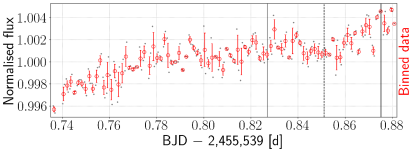
Figure 1: The raw light curve of WASP-43 system (HAWK-I, NB2090). The normalised raw light curve showing all data (the grey points) and data binned per 2 minutes (the red circles with error bars) is depicted. The vertical lines show the calculated beginning, the centre, and the end of the occultation.

3 Analysis of the photometric light curves

In this section we describe the fitting methods used for all our data sets to derive occultation depths. We also present here the basic equations to theoretically estimate the occultation depth both from the reflected light and from thermal emission.

3.1 The fitting routines and detrending

To fit the data sets, we used two different software packages. For fitting the TESS phase curves, we used allesfitter package and for fitting the HAWK-I data set we used GeePea modelling routine. These two methods are described in the following subsections.

3.1.1 ‘Allesfitter’ software package

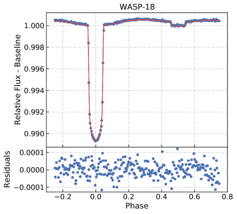
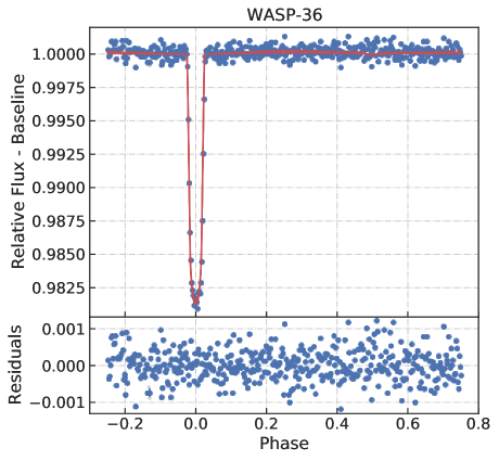
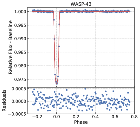
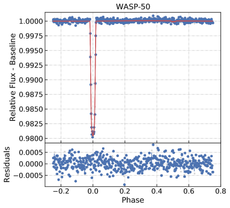
Figure 4: TESS phase curves fitted by allesfitter software package. The light grey points are the original data binned per 5 minutes, the blue points with error bars (mostly not visible) are the data binned per 15 minutes, and the red curves (seen as one) show 50 models which are randomly drawn from the posteriors.

To fit the TESS phase curves, shown in Fig. 4, we used python-based allesfitter software package (Günther & Daylan, 2019, 2021). It was developed to model photometric and radial velocity data. To make systematic noise models, Gaussian processes (GP) are included. After running the code an initial guess is obtained, then inference via MCMC or Nested Sampling is initiated. The methods include tests to assess convergence and also residual diagnostics to check possible structure in residuals. For details about allesfitter modelling package, see Günther & Daylan (2019, 2021) and the official website.

We fitted and sampled from the posterior of the ratio of the planetary to the stellar radius $R_{\mathrm{p}}/R_{\star}$, the sum of those radii divided by the semi-major axis $(R_{\mathrm{p}}+R_{\star})/a$, cosine of the inclination angle of the planetary orbit $\cos{i}$, epoch, i.e., the time of the centre of the transit $T_{0}$, the ratio of the surface brightness of the planet to the star $J$, logarithm of the error scaling of white noise used for the GP $\ln\sigma$, a baseline offset $\Delta{F}$, the semi-amplitude of the Doppler-boosting $A_{\mathrm{beaming}}$, the amplitude of the atmospheric contribution (both thermal and reflected) to the phase curve modulation $A_{\mathrm{atmospheric}}$, and the amplitude of the ellipsoidal modulation caused by tidal interaction between the host star and the planet $A_{\mathrm{ellipsoidal}}$. We fixed the orbital period of the planet $P$, eccentricity and argument of periastron (planetary orbit) $\sqrt{e}\cos{\omega}$ and $\sqrt{e}\sin{\omega}$, and limb darkening coefficients $q_{1}$ and $q_{2}$. The values of $P,e$, and $\omega$ were adopted from discovery articles of the particular exoplanetary systems (Table 1). To derive limb darkening coefficients we used the quadratic model of PyLDTk software package (Parviainen & Aigrain 2015 describing the package and Husser et al. 2013 describing the spectrum library).

The derived parameters from our fits were the host star radius divided by the semi-major axis $R_{\star}/a$, the semi-major axis divided by the host star radius $a/R_{\star}$, the planetary radius divided by the semi-major axis $R_{\mathrm{p}}/a$, the planetary radius $R_{\mathrm{p}}$, the semi-major axis of the planetary orbit $a$, the inclination angle of the planetary orbit $i$, the transit and occultation impact parameter $b_{\mathrm{tra}}$ and $b_{\mathrm{occ}}$, the total and full-transit duration $T_{\mathrm{tot}}$ and $T_{\mathrm{full}}$, the epoch of the occultation $T_{\mathrm{0;occ}}$, the equilibrium temperature of the planet $T_{\mathrm{eq;p}}$, the transit and occultation depth $\delta_{\mathrm{tra}}$ and $\delta_{\mathrm{occ}}$, the nightside flux of the planet $F_{\mathrm{nightside;p}}$, and host star density $\rho_{\star}$. Formulae of all derived parameters by allesfitter are listed in Table A3 of Günther & Daylan (2021).

We used all the TESS photometric data of the systems available to date. Particularly, for WASP-18 modelling we used data of sectors 2, 3, 29, and 30, for WASP-36 data of sectors 8 and 34, for WASP-43 data of sectors 9 and 35, for WASP-50 data of sectors 4 and 31, and for WASP-51 data of sectors 7 and 34. For each sector of every system we period-folded the light curves and then merged all the light curves of each system together. Finally, we binned the data sets per 5-minute time intervals.

For each modelling, we used both MCMC and Nested Sampling method to fit our data and to derive parameters and their uncertainties. Both the methods perfectly agreed and gave results with negligible differences. As Nested Sampling ensures that all convergence criteria are fulfilled, we present only the results obtained from this method (Section 4.1).

3.1.2 ‘GeePea’ routine

For fitting our HAWK-I data set (WASP-43), we used a Gaussian Processes method. The method is defined as an infinite set of Gaussian variables which have common Gaussian distribution. The systematics are modelled here as a stochastic process. The GP model, our eclipse model, is a set of a deterministic component and a stochastic component. These are represented here as a mean function (the light-curve model) and a kernel function (the noise model), respectively. To implement our GP, we used the GeePea code as described in Gibson et al. (2013a, 2013b) and Gibson (2014).

If we model a light curve of transit or occultation by using the GP, we have to assign parameters to the mean and kernel function (we will refer the parameters of the kernel function to ‘hyperparameters’). The kernel function takes at least three hyperparameters: height scale $\xi$ physically representing the typical range of the data points on the y-axis, a vector of length scale parameters $\eta$ physically representing changes on the x-axis (distance between ‘bumps’), and white noise $\sigma^{2}_{\mathrm{w}}$. We assign an array of parameters to the mean function, which represents the light-curve model. These parameters are time of the occultation centre $T_{0}$, orbital period $P$, scaled semi-major axis $a/R_{\star}$, planet-star radii ratio $R_{\mathrm{p}}/R_{\star}$, impact parameter $b$, out-of-transit flux $f_{\mathrm{oot}}$, time gradient $T_{\mathrm{grad}}$, expected occultation depth $\delta_{\mathrm{occ}}$ and, in the case of a primary transit, also limb darkening coefficients $q_{1}$ and $q_{2}$. As the HAWK-I data are obtained only during the planetary occultation, we fitted only the occultation.

Before the run of the fitting routine, $P$, $a/R_{\star}$, $R_{\mathrm{p}}/R_{\star}$, and $b$ were taken from literature and thus fixed. The fitted parameters were $T_{0}$, $f_{\mathrm{oot}}$, $T_{\mathrm{grad}}$, $\delta_{\mathrm{occ}}$, and hyperparameters of the kernel function $\xi$, $\eta$, and $\sigma^{2}_{\mathrm{w}}$. In our case, besides time ($\eta_{t}$), we used airmass ($\eta_{a}$) as the second component of the length scale vector $\eta$.

To detrend the fitted light curve, we used polynomial regression of degree two assuming the out-of-occultation model to be a quadratic function of time ($f(t)=at^{2}+bt+c$). For the polynomial regression we excluded data during the occultation. After inferring their values we calculated the function $f(t)$ for all the data points. To get the detrended and normalised-to-one flux and the occultation model, we subsequently divided our data by the the polynomial function.

We describe results of the HAWK-I light curve fit of WASP-43 in Section 4.2.

3.2 Occultation depth estimation

One of the input parameters of the GeePea routine is an estimated flux drop during the occultation searched in our data which is then refined by the routine. The value is also needed to interpret the data and compare it with atmospheric models. To get the flux drop estimation, we used a formula to calculate the occultation depth caused by reflected light (by a Lambert surface, i.e., a surface which scatters intensity isotropically; e.g., Winn, 2010):

$$\delta_{\mathrm{occ,re}}=A_{\mathrm{g}}\left(\frac{R_{\mathrm{p}}}{a}\right)^{2},$$ (1)

where $A_{\mathrm{g}}$ is the wavelength dependent geometric albedo (ratio of the flux of a planet at full phase to the flux of a perfectly diffusing Lambert disc), $R_{\mathrm{p}}$ is the planetary radius and $a$ is the semi-major axis of the orbit. For putting upper limits on occultation depths we assume $A_{\mathrm{g}}$ equal to one which sets the maximum possible value of the occultation depth due to reflected light.

During an occultation, the radiation flux of the system is decreased as the thermal radiation from the planet is no longer seen while the planet is behind the star. To include that, we used the following formulation to estimate the thermal contribution of the planet:

$$\delta_{\mathrm{occ,th}}=\left(\frac{R_{\mathrm{p}}}{R_{\star}}\right)^{2}\frac{B_{\lambda}(T_{\mathrm{p}})}{B_{\lambda}(T_{\star})},$$ (2)

where $R_{\star}$ is the stellar radius and $B_{\lambda}$ ($T_{\mathrm{p}},T_{\star}$) are the Planck’s functions corresponding to temperatures of the planet ($T_{\mathrm{eq}}$) and the star ($T_{\mathrm{e{f}f,\star}}$), approximating them as blackbody radiators.

3.3 Estimation of temperatures

To estimate the equilibrium temperature of a planet we used this formula:

$$T_{\mathrm{eq,p}}=T_{\mathrm{e{f}f,\star}}\sqrt{\frac{R_{\star}}{a}}\sqrt[4]{f(1-A_{\mathrm{B}})}.$$ (3)

Here $T_{\mathrm{e{f}f,\star}}$ is the effective temperature of the parent star, $R_{\star}$ is its radius, $A_{\mathrm{B}}$ is the Bond albedo (including radiation at all frequencies scattered into all directions), and $f$ is a flux correction factor connected with redistribution of the stellar radiation over the planet’s hemispheres.

Knowing the occultation depth from our fit and approximating planets and stars to be blackbody radiators, the brightness temperature $T_{\mathrm{b}}$ can be calculated from the occultation depth $\delta_{\mathrm{occ}}$ as follows:

$$T_{\mathrm{b}}(\lambda)=\left(\frac{\mathrm{hc}}{\lambda\mathrm{k}_{\mathrm{B}}}\right)\left\lgroup\ln\left(1+\frac{2\mathrm{h}\mathrm{c}^{2}k^{2}}{\delta_{\mathrm{occ}}\lambda^{5}B_{\lambda,\star}}\right)\right\rgroup^{-1},$$ (4)

where h is Planck’s constant, c is the speed of light in vacuum, k_B is the Steffan-Boltzmann constant, $\lambda$ is the wavelength at which we observed, $\delta_{\mathrm{occ}}$ is the measured occultation depth, and $B_{\lambda,\star}$ is the Planck function corresponding to $T_{\mathrm{e{f}f}}$ of the star. We have also denoted $k^{2}\equiv\left(R_{\mathrm{p}}/R_{\star}\right)^{2}$ and used the wavelength dependent form of the Planck’s law.

4 Results

Following the methods described in Section 3, in Section 4.1 we describe our results for the TESS phase curves for each hot Jupiter target and in Section 4.2 for the HAWK-I occultation for WASP-43 b.

4.1 TESS phase curve models and upper limits

We were able to detect primary transits of all the systems in the TESS data sets. We have also detected the occultation of WASP-18 b, which has the brightest host star among the systems we consider here. For the other systems we were able to place upper limits on their occultation depths and corresponding upper limits on their geometric albedos. For each binned data set we have also calculated the standard deviation of the weighted mean (RMS_w), serving as a measure of the quality of the data set and which can also be compared with expected and derived occultation depths.

To derive $3\sigma$ upper limits on the occultation depths of WASP-36 b, WASP-43 b, WASP-50 b, and WASP-51 b, we took values of the upper and the lower uncertainties of the derived occultation depth, averaged them, and multipied by three (i.e., $3[(\sigma_{+}+\sigma_{-})/2]$). A corresponding upper limit on the geometric albedo can be obtained using Equation 1 and by estimating the contribution of reflected light, $\delta_{\mathrm{occ,re}}$, to the observed occultation depth. To do this, we use Equation 2 to estimate the contribution of thermal emission to the occultation depth, and subtract it from the observed occultation depth: $\delta_{\mathrm{occ,re}}=\delta_{\mathrm{occ}}-\delta_{\mathrm{occ,th}}$.

In Table 2, we summarise our constraints on the transit/occultation depths and geometric albedos of each planet. We also show ‘expected’ values of the occultation depth for each planet ($\delta_{\mathrm{occ,exp}}$), calculated as the sum of the ‘expected’ occultation depths due to reflected light ($\delta_{\mathrm{occ,re,exp}}$) and thermal emission ($\delta_{\mathrm{occ,th,exp}}$). These contributions are defined by Equations 1 and 2, respectively, assuming a limiting case of $A_{\mathrm{g}}=1$ and $T_{\mathrm{p}}=T_{\mathrm{eq,p}}$, where $T_{\mathrm{eq,p}}$ is defined according to Equation 3 with $f=0.25$ and $A_{\mathrm{B}}=0$. For all five hot Jupiters considered here, the occultation depth constraint (whether a detection or an upper limit) is lower than the ‘expected’ occultation depth due to reflection alone, $\delta_{\mathrm{occ,re,exp}}$. This indicates that $A_{\mathrm{g}}<1$ for these planets, as expected given existing constraints on hot Jupiter albedos (e.g., Esteves et al., 2015). Fig. 2 shows our derived geometric albedo constraints as a function of $a/R_{\mathrm{p}}$ for all the planets studied in this work, alongside existing optical albedo constraints from the literature. The ratio $a/R_{\mathrm{p}}$ can be used to identify how well an exoplanet fits the characteristics of a hot Jupiter; a lower value means that the planet is closer to its parent star and/or has a larger radius.

In Fig. 3, we show geometric albedo as a function of equilibrium temperature for the same planets as in Fig. 2. The geometric albedo upper limits which we derive in this work for WASP-18 b, WASP-36 b, WASP-43 b, WASP-50 b, and WASP-51 b all lie below 0.45. This is consistent with previous works which find that hot Jupiters typically have low albedos (e.g., Heng & Demory, 2013; Esteves et al., 2015; Mallonn et al., 2019; Brandeker et al., 2022), though higher optical albedos have also been measured in some cases (e.g., Esteves et al., 2015; Niraula et al., 2018; Wong et al., 2020b; Adams et al., 2021; Heng et al., 2021). The geometric albedos shown in Fig. 3 are consistent with a range of values, with upper limits spanning $\lesssim 0.05$ to $\sim 0.45$. The diversity seen in hot Jupiter albedos may be indicative of a variety of cloud types and processes (Adams et al., 2021). Future albedo measurements spanning a wider range of equilibrium temperatures will be needed to further elucidate the nature of optical scattering in hot Jupiter atmospheres.

In what follows, we describe our results from the TESS data for each planet in turn. The estimated values of the fitted parameters are shown in Table 2, alongside the fixed parameters. In Table 2, we summarise the parameters subsequently derived from the best-fitting phase curve parameters. Fig. 4 and 5 show the fitted phase curves and occultations, respectively.

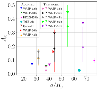
Figure 2: Optical geometric albedo as a function of the semi-major axis to planetary radius ratio, $a/R_{\textrm{p}}$. We include albedo constraints from the literature for seven hot Jupiters (‘Adopted’) as well as the TESS albedos derived here for WASP-18 b, WASP-36 b, WASP-43 b, WASP-50 b, and WASP-51 b (‘This work’). The downward triangles ($\blacktriangledown$) show upper limits while a different symbol (bold ‘+’ for our results) with an error bar shows a derived value including uncertainties. Literature references and corresponding instruments used are: WASP-12 b: Bell et al. (2017), HST STIS; WASP-18 b: Shporer et al. (2019), TESS; HD 209458 b: Brandeker et al. (2022), CHEOPS; TrES-2 b: Kipping & Spiegel (2011), Kepler; Qatar-2 b: Dai et al. (2017), K2 (Kepler); WASP-36 b & WASP-43 b: Wong et al. (2020b), TESS.

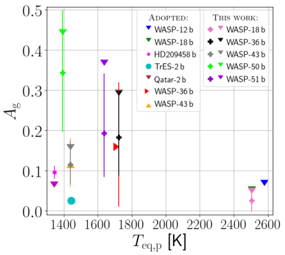
Figure 3: Optical geometric albedo as a function of equilibrium temperature, $T_{\textrm{eq,p}}$, for the same planets as in Fig. 2. Meaning of the used symbols, literature references and instruments used are the same as in Fig. 2.

4.1.1 WASP-18

The TESS phase curve of this system has previously been studied by Shporer et al. (2019), as well as Günther & Daylan (2021) who also used allesfitter to fit the phase curve. We detected a primary transit depth of $10.617_{-0.015}^{+0.014}$ ppt and an occultation depth of $0.345\pm 0.011$ ppt. The occultation depth is consistent with the values derived by both Shporer et al. (2019) and Günther & Daylan (2021), while the primary transit depth we derive is consistent with that of Günther & Daylan (2021). Shporer et al. (2019) obtain a transit depth of 9.439${}^{+0.027}_{-0.026}$ ppt; the discrepancy between our value and theirs may be due to different analysis methods and the fact that we used data from four TESS sectors, while only two sectors were available at the time of their study. We determined the amplitude of the atmospheric contribution to the phase-curve model to be $0.3065\pm 0.0086$ ppt (i.e., a semi-amplitude of $0.1533\pm 0.0043$ ppt), which lies between the values derived by Günther & Daylan (2021) and Shporer et al. (2019). Furthermore, our value is consistent with that of Günther & Daylan (2021) to within $2\sigma$, which is expected since allesfitter was used for both analyses.

We further estimate the optical albedo of WASP-18 b based on the measured occultation depth. Due to the high dayside temperature of WASP-18 b, its thermal emission represents a non-negligible contribution in the TESS band, unlike the cooler targets in our sample. The way in which this thermal contribution is estimated may therefore have a significant effect on the resulting albedo constraint. Using Equation 2, the thermal contribution to the occultation depth in the TESS band is 97 ppm, resulting in an albedo value of $A_{\mathrm{g}}=0.340\pm 0.044$. This albedo calculation assumes efficient day-night energy redistribution ($f=0.25$) in the estimation of $T_{\mathrm{p}}$. However, existing infrared observations of WASP-18 b indicate that its day-night energy redistribution is inefficient (e.g., Arcangeli et al. 2018, see also Section 5).

A more accurate albedo constraint can be derived by considering a more realistic thermal contribution to the TESS occultation depth. Shporer et al. (2019) used the atmospheric model of Arcangeli et al. (2018), found by fitting the HST and Spitzer occultation depths of WASP-18 b and resulting in a thermal contribution of 0.327 ppt. As noted by Shporer et al. (2019), this contribution is consistent with the observed occultation depth, meaning that only an upper limit can be placed on the reflected contribution. They placed a $2\sigma$ upper limit of $A_{\mathrm{g}}<0.048$. To derive the geometric albedo, we used our value of the detected occultation depth and their value of the thermal contribution of 0.327 ppt, and we come to $A_{\mathrm{g}}=0.025\pm 0.027$ which is consistent with their value obtained from the upper limit on the occultation depth. The high values of the uncertainties are caused by uncertainties of the thermal contribution which are expected to be a few per cent using the model of Arcangeli et al. 2018 as in Shporer et al. (2019). Thus, we set them to be 5 per cent when calculating the geometric albedo uncertainties. However, as our detected occultation depth is very similar to theirs (0.345 vs 0.341 ppt), we can also not claim a detection of the reflected light since the difference between the thermal emission and our occultation depth is not at $3\sigma$ significance ($\sim 1.6\sigma$). We, therefore, set a $3\sigma$ uppper limit on the reflected light by the planet of $<0.033$ ppt implying an upper limit on the geometric albedo $A_{\mathrm{g}}<0.045$, consistent with the $2\sigma$ upper limit of Shporer et al. 2019.

We note that our self-consistent atmospheric model for WASP-18 b, discussed in Section 5, is consistent with the observed occultation depth within 2$\sigma$ without the inclusion of scattering from clouds or hazes. The predicted thermal contribution from this model is slightly higher than the observed occultation depth, and is therefore consistent with zero albedo in the TESS band.

4.1.2 WASP-36

We detected the primary transit of WASP-36 b and obtained a transit depth of $18.67\pm 0.13$ ppt. This value is lower than that obtained by Maciejewski et al. (2016) in the $R$-band ($19.349\pm 0.320$ ppt), however this difference may be due to the different wavelength range used. We obtained an occultation depth of $0.105^{+0.057}_{-0.049}$ ppt, and therefore did not significantly detect the occultation of WASP-36 b ($\sim 2\sigma$ detection). This is a result of the relatively high RMS_w of the data of 0.288 ppt. We place a 3$\sigma$ upper limit on the occultation depth of $\delta_{\mathrm{occ}}<0.159$ ppt. This is consistent with the constraint from Wong et al. (2020b), who derive $\delta_{\mathrm{occ}}=0.09^{+0.10}_{-0.07}$ ppt using TESS. Zhou et al. (2015) derive an occultation depth of $1.3\pm 0.4$ ppt in the $Ks$-band; for the shorter wavelengths at which TESS operates, the occultation depth is indeed expected to be lower under the assumption of little or no optical scattering. The upper limit which we derive on the occultation depth corresponds to a $3\sigma$ upper limit on the geometric albedo of $A_{\mathrm{g}}<0.286$. This is consistent with the geometric albedo constraint derived by Wong et al. (2020b) ($A_{\mathrm{g}}=0.16^{+0.16}_{-0.15}$).

4.1.3 WASP-43

We detected the primary transit of WASP-43 b, obtaining a transit depth of $26.597^{+0.078}_{-0.070}$ ppt. This value is slightly different than $25.415\pm 0.131$ ppt in the optical band ($i^{\prime}+g^{\prime}$ filters) published in Hoyer et al. (2016). We do not detect the occultation of WASP-43 b at sufficiently high significance, obtaining $\delta_{\mathrm{occ}}=0.123^{+0.059}_{-0.048}$ ppt ($2.3\sigma$) while the RMS_w of our data is 0.148 ppt. This is consistent with the results of Wong et al. (2020b), who obtain a TESS occultation depth of $\delta_{\mathrm{occ}}=0.17\pm 0.07$ ppt. Furthermore, Chen et al. (2014) measured the occultation depth of WASP-43 b in the $i^{\prime}$ band (centred on roughly the same wavelength as the TESS bandpass) to be $\delta_{\mathrm{occ}}=0.37\pm 0.22$ ppt, which is also consistent with our value. Fraine et al. (2021) put for the reflected light component a $3\sigma$ upper limit $\delta_{\mathrm{occ}}<0.067$ ppt from HST WFC3/UVIS data and from this value they derived a $3\sigma$ upper limit $A_{\mathrm{g}}\lesssim 0.06$. From our $3\sigma$ upper limit on the occultation depth of $\delta_{\mathrm{occ}}<0.161$ ppt, we derive an upper limit on the geometric albedo of $A_{\mathrm{g}}<0.154$. This value is consistent with the albedos derived by Wong et al. (2020b) and Chen et al. (2014), i.e., $0.12\pm 0.06$ and $0.31\pm 0.22$, respectively. Our $\delta_{\mathrm{occ}}$ and $A_{\mathrm{g}}$ upper limits are also consistent with the upper limits obtained by Fraine et al. (2021).

4.1.4 WASP-50

We obtained a transit depth value of $19.502^{+0.085}_{-0.093}$ ppt. This is consistent with the derived value of $19.321\pm 0.167$ ppt in the $I$ and $R$ bands published in Chakrabarty & Sengupta (2019). We detected an occultation with less than $3\sigma$ significance, $\delta_{\mathrm{occ}}=0.117^{+0.051}_{-0.048}$ ppt ($\sim 2.4\sigma$), which is nevertheless the first occultation measurement of this system. Our derived value is lower than the expected value of 0.342 ppt (assuming $A_{g}=1$) and also lower than RMS_w of our data, 0.174 ppt. We placed a $3\sigma$ upper limit on the occultation depth $\delta_{\mathrm{occ}}<0.149$ ppt. From the upper limit of the occultation depth, we then derived an upper limit on the geometric albedo of $A_{\mathrm{g}}<0.44$.

4.1.5 WASP-51

We obtained a transit depth of $10.872\pm 0.055$ ppt. While this value is not consistent with the transit depths derived by Maciejewski et al. (2016) and Saha et al. (2021) in the $R$ and $V$ bands, respectively, the difference may be due to the use of different wavelength ranges. Indeed, Saeed et al. (2022) discovered a strong dependency of the transit depth with wavelength. The occultation of WASP-51 b was not detected at sufficiently high significance, with a measured occultation depth of $0.048^{+0.033}_{-0.024}$ ppt ($\sim 1.7\sigma$). As in the case of WASP-50, this the first occultation measurement of this system. The RMS of the data was also high, at 0.105 ppt. We placed an upper limit on the occultation depth $\delta_{\mathrm{occ}}<0.086$ ppt. This allowed us to set a $3\sigma$ upper limit on the geometric albedo $A_{\mathrm{g}}<0.368$ ppt.

Table 2: Results of the analysed data sets. Parameters presented and their meaning is following: the used HAWK-I filter, RMS_w is the standard deviation of the weighted mean of the binned data sets, $\delta_{\mathrm{occ,re,exp}}$ is the expected occultation depth due to reflected light, $\delta_{\mathrm{occ,th,exp}}$ is the expected occultation depth due to thermal radiation, $\delta_{\mathrm{occ,exp}}$ is the total expected occultation depth (the sum of the both previous), $\delta_{\mathrm{occ}}$ is the derived occultation depth (with at least $3\sigma$ significance), $\delta_{\mathrm{occ,}3\sigma\mathrm{UL}}$ is the $3\sigma$ upper limit on the occultation depth, and $A_{\mathrm{g}}$ is the upper limit (or derived value) of the geometric albedo. For TESS data sets $\delta_{\mathrm{tra}}$ is the inferred transit depth. In the third table $T_{\mathrm{eq,p}}$ is the equilibrium temperature of the planet. Notes: ^(a): calculated from Equation 1 supposing $A_{\mathrm{g}}=1$; ^(b): calculated from Equation 2 substituting $T_{\mathrm{p}}=T_{\mathrm{eq,p}}$ and $T_{\star}=T_{\mathrm{e{f}f,\star}}$; ^(c): adopted from Arcangeli et al. (2018), as in Shporer et al. (2019); ^(d): derived using the thermal contribution from Arcangeli et al. (2018), as in Shporer et al. (2019); ^(e): calculated from Equation 3 assuming $f=1/4$ and $A_{\mathrm{B}}=0$.

TESS data sets
System	$\delta_{\mathrm{tra}}$	RMSw	$\delta_{\mathrm{occ,re,exp}}$ (a)	$\delta_{\mathrm{occ,th,exp}}$ (b)	$\delta_{\mathrm{occ,exp}}$	$\delta_{\mathrm{occ}}$	$A_{\mathrm{g}}$	$\delta_{\mathrm{occ,3\sigma UL}}$	$A_{\mathrm{g,3\sigma UL}}$
	[ppt]	[ppt]	[ppt]	[ppt]	[ppt]	[ppt]		[ppt]
WASP-18	$10.617_{-0.015}^{+0.014}$	0.042	0.690	0.327(c)	1.017	$0.345_{-0.011}^{+0.011}$	$0.025^{+0.027~{}(d)}_{-0.027}$	–	$<0.045^{(d)}$
WASP-36	$18.670^{+0.130}_{-0.130}$	0.288	0.500	0.012	0.512	$0.105_{-0.049}^{+0.057}$	$0.181^{+0.112}_{-0.096}$	$<0.159$	$<0.286$
WASP-43	$26.597_{-0.070}^{+0.078}$	0.148	0.990	0.007	0.997	$0.123_{-0.048}^{+0.059}$	$0.116^{+0.059}_{-0.048}$	$<0.161$	$<0.154$
WASP-50	$19.502_{-0.093}^{+0.085}$	0.174	0.340	0.002	0.342	$0.117_{-0.048}^{+0.051}$	$0.344^{+0.156}_{-0.148}$	$<0.149$	$<0.440$
WASP-51	$10.872^{+0.055}_{-0.055}$	0.105	0.263	0.004	0.267	$0.048_{-0.024}^{+0.033}$	$0.197^{+0.149}_{-0.109}$	$<0.086$	$<0.368$

VLT HAWK-I data set
System	Filter	RMSw [ppt]	$\delta_{\mathrm{occ,re,exp}}$ [ppt](a)	$\delta_{\mathrm{occ,th,exp}}$ [ppt](b)	$\delta_{\mathrm{occ,exp}}$ [ppt]	$\delta_{\mathrm{occ}}$ [ppt]
WASP-43	NB2090	0.298	0.990	0.750	1.740	$1.26^{+0.17}_{-0.17}$

Planet:	WASP-18 b	WASP-36 b	WASP-43 b	WASP-50 b	WASP-51 b
$T_{\mathrm{eq}}$ [K](e)	$2504^{+63}_{-65}$	$1724^{+43}_{-43}$	$1439^{+34}_{-31}$	$1393^{+42}_{-42}$	$1637^{+42}_{-42}$

=1.33in Posterior values of all the fitted parameters (and hyperparameters) of TESS phase curves of all the systems analysed in this work obtained by using by allesfitter NS. Parameter / System WASP-18 WASP-36 WASP-43 WASP-50 WASP-51 fit/fixed $R_{\mathrm{p}}/R_{\star}$ $0.09669\pm 0.00013$ $0.13271\pm 0.00085$ $0.15865\pm 0.00044$ $0.13668\pm 0.00058$ $0.10949\pm 0.00046$ fit $(R_{\star}+R_{\mathrm{p}})/a$ $0.3131\pm 0.0023$ $0.1952\pm 0.0044$ $0.2474\pm 0.0022$ $0.1550\pm 0.0022$ $0.1609\pm 0.0013$ fit $\cos{i}$ $0.0997_{-0.0063}^{+0.0059}$ $0.1157\pm 0.0059$ $0.1481\pm 0.0027$ $0.0974\pm 0.0028$ $0.1214\pm 0.0013$ fit $T_{0}$ [epoch] $0.000021\pm 0.000035$ $-0.00002\pm 0.00014$ $0.000013\pm 0.000048$ $-0.000017\pm 0.000096$ $0.00004\pm 0.00012$ fit $P$ [d] $0.9414518$ $1.5373653$ $0.81347753$ $1.9550959$ $2.8106084$ fixed $\sqrt{e}\cos{\omega}$ $-0.00163718$ $0.0$ $0.05017120$ $0.06824257$ $-0.05781180$ fixed $\sqrt{e}\sin{\omega}$ $-0.09379403$ $0.0$ $-0.03135045$ $0.06590108$ $-0.17792638$ fixed $J_{\mathrm{TESS}}$ $0.0041\pm 0.0012$ $0.0019_{-0.0013}^{+0.0024}$ $0.0032_{-0.0018}^{+0.0022}$ $0.0035_{-0.0021}^{+0.0029}$ $0.0037_{-0.0021}^{+0.0026}$ fit $q_{1;~{}\mathrm{TESS}}$ $0.36660057$ $0.38667813$ $0.53140888$ $0.44026143$ $0.37665187$ fixed $q_{2;~{}\mathrm{TESS}}$ $0.15570471$ $0.15819508$ $0.10952400$ $0.13763435$ $0.1549222$ fixed $\ln\sigma_{\mathrm{TESS}}$ [ln(relative flux)] $-10.075\pm 0.043$ $-7.774\pm 0.034$ $-8.605\pm 0.048$ $-8.245\pm 0.030$ $-8.732\pm 0.026$ fit $\Delta F_{\mathrm{TESS}}$ $-0.0002474\pm 0.0000076$ $0.000141_{-0.000040}^{+0.000038}$ $0.000161_{-0.000027}^{+0.000025}$ $0.000050_{-0.000019}^{+0.000017}$ $0.0000334\pm 0.0000099$ fit $A_{\mathrm{p;~{}beaming;~{}TESS}}$ [ppt] (semi-amplitude) $0.0312\pm 0.0035$ $0.032_{-0.018}^{+0.024}$ $0.0157_{-0.0096}^{+0.013}$ $0.033_{-0.014}^{+0.015}$ $0.0139_{-0.0069}^{+0.0074}$ fit $A_{\mathrm{p;~{}atmospheric;~{}TESS}}$ [ppt] (amplitude) $0.3065\pm 0.0086$ $0.062_{-0.036}^{+0.049}$ $0.037_{-0.022}^{+0.030}$ $0.044_{-0.024}^{+0.030}$ $0.0031_{-0.0022}^{+0.0042}$ fit $A_{\mathrm{p;~{}ellipsoidal;~{}TESS}}$ [ppt] (amplitude) $0.3516\pm 0.0089$ $0.099_{-0.050}^{+0.058}$ $0.085\pm 0.037$ $0.0084_{-0.0057}^{+0.0110}$ $0.026_{-0.014}^{+0.016}$ fit =1.3in Posterior values of all the derived parameters of TESS phase curves of all the systems analysed in this work obtained by using by allesfitter NS. Parameter / System WASP-18 WASP-36 WASP-43 WASP-50 WASP-51 Host star radius over semi-major axis; $R_{\star}/a$ $0.2855\pm 0.0021$ $0.1723\pm 0.0038$ $0.2135\pm 0.0018$ $0.1364\pm 0.0019$ $0.1450\pm 0.0012$ Semi-major axis over host star radius; $a/R_{\star}$ $3.502\pm 0.025$ $5.80_{-0.12}^{+0.13}$ $4.683\pm 0.041$ $7.33\pm 0.11$ $6.895\pm 0.056$ Planetary radius over semi-major axis; $R_{\mathrm{p}}/a$ $0.02761\pm 0.00023$ $0.02286\pm 0.00062$ $0.03388\pm 0.00037$ $0.01864\pm 0.00033$ $0.01588\pm 0.00018$ Planetary radius; $R_{\mathrm{p}}$ [$\mathrm{R_{\oplus}}$] $13.29\pm 0.42$ $13.6\pm 2.5$ $11.54\pm 0.18$ $13.1\pm 1.6$ $15.89\pm 0.37$ Planetary radius; $R_{\mathrm{p}}$ [$\mathrm{R_{J}}$] $1.186\pm 0.038$ $1.21\pm 0.22$ $1.030\pm 0.016$ $1.17\pm 0.15$ $1.417\pm 0.033$ Semi-major axis of the planetary orbit; $a$ [$\mathrm{R_{\odot}}$] $4.41\pm 0.14$ $5.46\pm 1.0$ $3.124\pm 0.054$ $6.45\pm 0.81$ $9.17\pm 0.22$ Semi-major axis of the planetary orbit; $a$ [au] $0.02052\pm 0.00067$ $0.0254\pm 0.0047$ $0.01453\pm 0.00025$ $0.0300\pm 0.0038$ $0.0427\pm 0.0010$ Inclination angle of the planetary orbit; $i$ [deg] $84.28_{-0.34}^{+0.37}$ $83.36\pm 0.34$ $81.49\pm 0.16$ $84.41\pm 0.16$ $83.026\pm 0.077$ Impact parameter; $b_{\mathrm{tra}}$ $0.352_{-0.020}^{+0.018}$ $0.671_{-0.020}^{+0.018}$ $0.6946\pm 0.0069$ $0.7099_{-0.0110}^{+0.0099}$ $0.8651\pm 0.0029$ Total transit duration; $T_{\mathrm{tot}}$ [h] $2.1956\pm 0.0041$ $1.867\pm 0.017$ $1.2552\pm 0.0058$ $1.810\pm 0.012$ $2.257\pm 0.011$ Full-transit duration; $T_{\mathrm{full}}$ [h] $1.7486\pm 0.0043$ $1.121_{-0.027}^{+0.025}$ $0.6393\pm 0.0091$ $1.000_{-0.019}^{+0.018}$ $0.686_{-0.039}^{+0.037}$ Epoch occultation; $T_{\mathrm{0;occ}}$ $0.470655\pm 0.000035$ $0.76867\pm 0.00014$ $0.408289\pm 0.000049$ $0.985589\pm 0.000096$ $1.38599\pm 0.00012$ Impact parameter occultation; $b_{\mathrm{occ}}$ $0.346_{-0.020}^{+0.018}$ $0.671_{-0.020}^{+0.018}$ $0.6921\pm 0.0069$ $0.7188_{-0.011}^{+0.0100}$ $0.8093\pm 0.0027$ Transit depth; $\delta_{\mathrm{tra;p;TESS}}$ [ppt] $10.617_{-0.015}^{+0.014}$ $18.67\pm 0.13$ $26.597_{-0.070}^{+0.078}$ $19.502_{-0.093}^{+0.085}$ $10.872\pm 0.055$ Occultation depth; $\delta_{\mathrm{occ;p;TESS}}$ [ppt] $0.345\pm 0.011$ $0.105_{-0.049}^{+0.057}$ $0.123_{-0.048}^{+0.059}$ $0.117_{-0.048}^{+0.051}$ $0.048_{-0.024}^{+0.033}$ Nightside flux of the planet; $F_{\mathrm{nightside;p;TESS}}$ [ppt] $0.039\pm 0.011$ $0.034_{-0.023}^{+0.043}$ $0.079_{-0.043}^{+0.057}$ $0.068_{-0.041}^{+0.047}$ $0.045_{-0.025}^{+0.031}$ Median host star density – all orbits; $\rho_{\mathrm{\star}}$ (cgs) $0.917\pm 0.020$ $1.564_{-0.096}^{+0.11}$ $2.936\pm 0.077$ $1.950_{-0.080}^{+0.086}$ $0.785\pm 0.019$

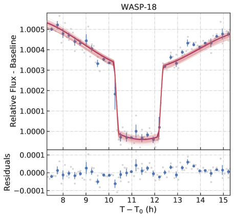
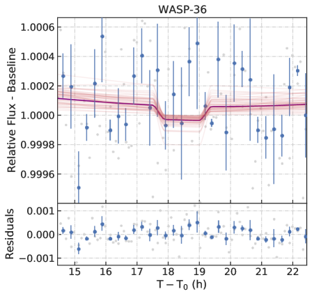
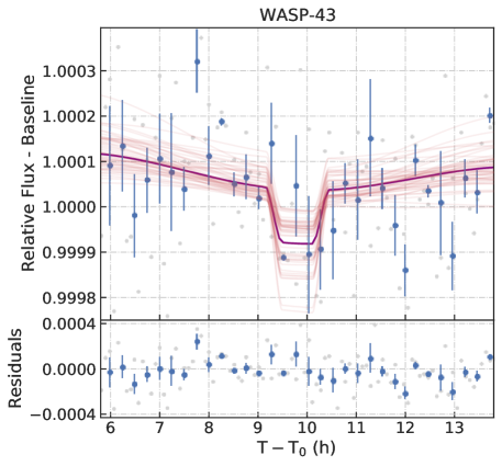
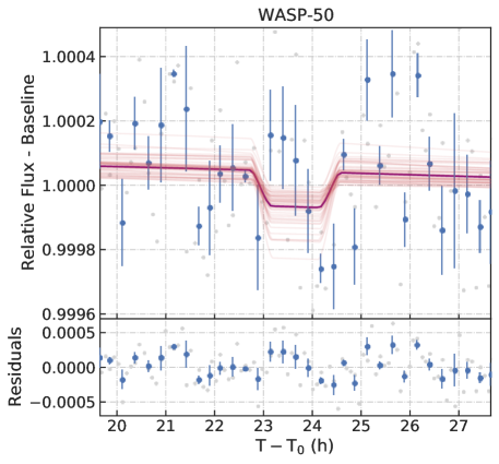
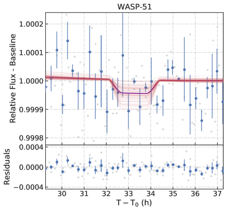
Figure 5: TESS phase curves fitted by allesfitter software package with the occultation part zoomed. The purple curves show the median model drawn from the posteriors. The meaning of all the points and the red curves is the same as in Fig. 4.

4.2 HAWK-I occultation measurement for WASP-43 b

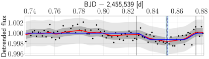
Figure 6: Results of the best-fitting model of WASP-43 from HAWK-I data. The upper panel: Detrended occultation light curve. The black dots are our measurements binned per 2 minutes, the red curve shows the fit of the data (the occultation model + noise model) together with $1\sigma$ and $3\sigma$ regions depicted as the shaded regions. The blue curve is the occultation model only. The black vertical lines show the calculated beginning, the centre, and the end of the occultation, and the blue dot-and-dash vertical line shows the inferred centre of the occultation together with $1\sigma$ uncertainty region (the light-blue area). The bottom panel: blue – residuals of the occultation model, red – residuals of the fit.

We detected the occultation of WASP-43 b using the HAWK-I NB2090 data described in Section 2.3.2, consistent with the detection by Gillon et al. (2012) who used the same data set but different analysis methods. Here, we first binned the near-infrared HAWK-I data by 2-minute time intervals. As well as for the TESS data sets, we have calculated the $\mathrm{RMS_{w}}$. The fitted light curve is shown in Fig. 6. All used and inferred parameters are summarised in Table 3.

We detected the occultation of WASP-43 b and inferred an occultation depth, $\delta_{\mathrm{occ}}$, of $1.26\pm 0.17$ ppt. The inferred time of the occultation centre is consistent with the expected value within the derived uncertainty. Our $\delta_{\mathrm{occ}}$ value is consistent with the value of Gillon et al. (2012) ($1.56\pm 0.14$ ppt) within $1.8\sigma$. Our inferred occultation depth of $1.26\pm 0.17$ ppt is significantly deeper than our TESS occultation depth upper limit of 0.161 ppt. This implies that planet-star flux ratio is increasing with wavelength, which is naturally explained by the decreasing stellar flux and increasing planetary thermal emission with wavelength in the near-infrared.

We use this occultation depth to calculate the brightness temperature of WASP-43 b at $\sim 2.09\,\upmu$m, obtaining a value of $T_{\mathrm{b}}=1619\pm 52$ K. This temperature can be used to gain some initial insights into the energy redistribution in the atmosphere of WASP-43 b. For example, the equilibrium temperature of WASP-43 b assuming zero albedo and a flux correction factor, $f$, of 1/4 is $T_{\mathrm{eq}}=1439\pm 34$ K (see Equation 3). The brightness temperature corresponding to the HAWK-I occultation is greater than $T_{\mathrm{eq}}$, which may be due to inefficient day-night energy redistribution (i.e., $f>1/4$). A lower limit on the efficiency of day-night energy redistribution can be estimated by substituting $T_{\mathrm{b}}-\sigma_{T_{\mathrm{b}}}$ for $T_{\mathrm{eq,p}}$ in Equation 3 and solving for $f$. We obtain a physically plausible estimate of $f\geq 0.35$, which lies between the limits of $f=1/4$ (uniform redistribution) and $f=2/3$ (instantaneous reradiation). This is consistent with the result obtained by Chen et al. (2014) of $f\geq 0.56$, measured in the $K$ band.

While optical observations can be used to estimate the optical albedos of hot Jupiter atmospheres, inferring infrared scattering can be more complex. In the near-infrared, thermal emission dominates the observed planetary flux and is expected to be significantly greater than the contribution from reflected light. Furthermore, molecular opacity in the infrared causes the planetary thermal emission to significantly deviate from a blackbody spectrum, as can be seen from the evident H₂O absorption in the HST/WFC3 spectrum of WASP-43 b (Kreidberg et al., 2014). As a result, the method described in Section 4.1 to estimate optical geometric albedos should not be used in the near-infrared. Instead, detailed radiative-convective atmospheric models can be used to explain multi-wavelength observations and assess the need for optical and/or infrared scattering. We do this for WASP-43 b and WASP-18 b in Section 5, and find that cloud scattering is not required to explain either of their optical to infrared spectra.

While our self-consistent atmospheric models indicate that cloud scattering is not needed to explain the optical and infrared observations of WASP-43 b, Keating & Cowan (2017) find that an infrared albedo of $0.24\pm 0.01$ is needed to fit the HST/WFC3 and Spitzer observations. However, we note that their atmospheric model assumes an isothermal temperature profile, which does not capture the effect of molecular absorption features. In contrast to this, we find that the HST/WFC3 and Spitzer data can be explained by absorption features due to H₂O and CO (see Section 5). This highlights the need to consider molecular spectral features when interpreting infrared observations. Nevertheless, in order to compare with the results of Keating & Cowan (2017), we use the HAWK-I occultation depth derived above to estimate a nominal infrared albedo. As in Keating & Cowan (2017), we assume a blackbody thermal contribution to the observed planetary flux. We use a planetary temperature of 1483 K, i.e., the best-fitting isothermal temperature found by Keating & Cowan (2017). Using Equation 2, this results in a nominal thermal contribution of 0.864 ppt. Following the methods outlined in Section 4.1, this results in an estimated infrared albedo of $A_{\mathrm{g}}=0.395^{+0.174}_{-0.176}$. Our nominal albedo estimate agrees with the results of Keating & Cowan (2017) when the same assumptions are made. However, we stress that the infrared thermal contribution should not be assumed to take the form of a blackbody, and that detailed atmospheric models are required to interpret infrared observations. We discuss our self-consistent models in Section 5.

Table 3: Deduced, calculated and fixed parameters of the occultation of WASP-43. Notes: ^(a): calculated from Equation 3 assuming $f=1/4$ and $A_{\mathrm{B}}=0$; ^(b): calculated from Equation 4; ^(c): taken from Hellier et al. (2011).

Deduced parameters:
occultation depth $\delta_{\mathrm{occ}}$ [ppt]	$1.261^{+0.165}_{-0.168}$
$T_{0}-2{,}450{,}000$ [BJDTDB]	$0.8519^{+0.0016}_{-0.0015}$
out-of-occultation flux $f_{\mathrm{oot}}$	$1.0027\pm 0.0003$
time gradient $T_{\mathrm{grad}}$	$0.0013\pm 0.0005$
time gradient $T^{2}_{\mathrm{grad}}$	$-0.0002\pm 0.0002$
$\xi$ (GP)	$0.0003877^{+0.0001523}_{-0.0001066}$
$\eta_{t}$ (GP)	$0.0081001^{+0.0018084}_{-0.0015249}$
$\eta_{a}$ (GP)	$0.0266166^{+0.0018885}_{-0.0017666}$
$\sigma_{\mathrm{w}}^{2}$ (GP)	$0.0007866^{+0.0000878}_{-0.0000703}$
Calculated parameters:
equilibrium temperature${}^{(a)}~{}T_{\mathrm{eq}}$ [K]	$1439^{+34}_{-31}$
brightness temperature${}^{(b)}~{}T_{\mathrm{b}}$ [K]	$1619^{+47}_{-52}$
Fixed parameters(c):
period $P$ [d]	0.81347404
scaled semi-major axis $a/R_{\star}$	5.13
ratio of the radii $R_{\mathrm{p}}/R_{\star}$	0.159687
impact parameter $b$	0.66

5 Atmospheric Constraints for WASP-43 b and WASP-18 b

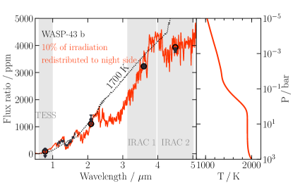
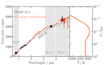
Figure 7: Self-consistent temperature profiles and thermal emission spectra for the dayside atmospheres of WASP-43 b (top panel) and WASP-18 b (bottom panel). TESS, HAWK-I and Spitzer observations (upper limits) are shown as black points and error bars (arrows), while the red circles show the binned model points. Note that the TESS error bar for WASP-18 b is smaller than the symbol size. The Spitzer data for WASP-43 b and WASP-18 b are from Blecic et al. (2014) and Sheppard et al. (2017), respectively. Small black points and error bars show HST/WFC3 data for WASP-43 b (Kreidberg et al., 2014) and WASP-18 b (Sheppard et al., 2017). The dashed black lines show blackbody spectra corresponding to the irradiation temperature, $T_{\rm irr}$, for each planet. $T_{\mathrm{irr}}=2^{-1/4}\sqrt{R_{\star}/a}\,T_{\rm e{f}f,\star}$ corresponds to the dayside temperature of the planet assuming no day-night energy redistribution and a Bond albedo of zero ($R_{\star}$, $a$, and $T_{\rm e{f}f,\star}$ defined as in Section 3).

WASP-43 b and WASP-18 b represent opposite ends in temperature across the hot and ultra-hot Jupiter regimes. Therefore, they are ideal case studies for the comparative study of hot Jupiter atmospheres, including the presence of clouds and hazes. The TESS and HAWK-I occultation depths we have derived for these planets (Section 4) provide constraints on the optical and near-infrared thermal emission/scattering of these planets. In this section, we therefore model the atmospheres of WASP-43 b and WASP-18 b in order to assess their potential atmospheric properties.

We self-consistently model the dayside atmospheres of WASP-43 b and WASP-18 b using the genesis atmospheric model (Gandhi & Madhusudhan, 2017; Piette et al., 2020). genesis solves for the temperature profile, thermal emission spectrum and chemical profile of the atmosphere by calculating full, line-by-line radiative transfer under radiative-convective, thermodynamic, hydrostatic and thermochemical equilibrium. In particular, equilibrium chemical abundances are calculated using the hsc chemistry (version 8) software (see e.g., Moriarty et al. 2014; Harrison et al. 2018; Piette et al. 2020). hsc chemistry minimizes the Gibbs’ free energy of the system using the gibbs solver (White et al., 1958), given the atmospheric elemental abundances. These equilibrium chemistry calculations consider $>150$ chemical species (see Piette et al. 2020). Of these, we consider atmospheric opacity due to the species known to dominate the H₂-rich atmospheres of hot Jupiters (Burrows & Sharp, 1999; Madhusudhan et al., 2016): H₂O, CH₄, CO, CO₂, NH₃, HCN, C₂H₂, Na, K, TiO, VO and H^-, besides H₂ and He. We note that besides Na, K, TiO and VO, other atomic and molecular species such as Fe and AlO can also contribute to the optical opacity and cause thermal inversions in hot Jupiter atmospheres (e.g., Lothringer et al., 2018; Gandhi & Madhusudhan, 2019). However, the optical data considered here (i.e., TESS photometry) is only sensitive to the integrated optical flux, and does not resolve spectral features due to individual species. We therefore use Na, K, TiO and VO as a proxy for the atmospheric optical opacity in these models, and find that we are able to explain the observations.

We calculate the absorption cross sections of these species as in Gandhi & Madhusudhan (2017) using line lists from ExoMol, HITEMP and HITRAN (H₂O, CO and CO₂: Rothman et al. 2010, CH₄: Yurchenko et al. 2013; Yurchenko & Tennyson 2014, C₂H₂: Rothman et al. 2013; Gordon et al. 2017, NH₃: Yurchenko et al. 2011, HCN: Harris et al. 2006; Barber et al. 2014, TiO: McKemmish et al. 2019, VO: McKemmish et al. 2016, H₂-H₂ and H₂-He Collision-Induced Absorption: Richard et al. 2012). Na and K opacities are calculated as in Burrows & Volobuyev (2003) and Gandhi & Madhusudhan (2017), and H^- bound-free and free-free cross sections are calculated using the prescriptions of Bell & Berrington (1987) and John (1988) (see also Arcangeli et al. 2018; Parmentier et al. 2018; Gandhi et al. 2020).

The free parameters in the atmospheric model are therefore the elemental abundances (explored here by changing the C/O ratio and metallicity), the incident irradiation, and the internal flux. The incident irradiation on the dayside of a hot Jupiter can be varied by considering different efficiencies of energy redistribution, both on the day side and between the day and night sides (see e.g., Burrows et al., 2008a), as described below. The internal flux can be parameterised by a single temperature parameter ($T_{\rm int}$) and represents the flux emanating from the planetary interior, e.g., as a remnant of the planet formation process. Given the relatively high irradiation levels of both WASP-43 b and WASP-18 b, the internal heat is not expected to noticeably affect the observable atmosphere. We therefore set $T_{\rm int}$ to a nominal value of 100 K, similar to that of Jupiter. We explore physically plausible models for WASP-43 b and WASP-18 b in order to explain their observed TESS and HAWK-I occultation depths (reported in this work) as well as existing Spitzer IRAC dayside fluxes. The IRAC 1 and IRAC 2 data are obtained from Blecic et al. (2014) and Sheppard et al. (2017) for WASP-43 b and WASP-18 b, respectively.

For WASP-43 b, we find that an atmospheric model with solar metallicity and $\mathrm{C/O}=0.5$ is able to fit the observed TESS, HAWK-I and Spitzer data if 10 per cent of the energy incident on the day side is transported to the night side, and energy redistribution is efficient on the dayside (top panel of Fig. 7). Using the notation of Burrows et al. (2008a) and Equation 3, this corresponds to a flux distribution factor of $f=0.45$. Our model is in agreement with previous inferences of inefficient day-night energy redistribution from Spitzer and TRAPPIST eclipse observations (Gillon et al., 2012; Blecic et al., 2014). The strong day-night flux contrast from Spitzer phase curve constraints is also suggestive of inefficient day-night energy redistribution (Stevenson et al., 2014, 2017), though Stevenson et al. (2017) note that this contrast could also be caused by high-altitude nightside clouds. Our model fits the Spitzer and HAWK-I NB2090 data within the $\sim 1\sigma$ uncertainties, while models with more efficient day-night energy redistribution result in IRAC 1 and IRAC 2 brightness temperatures which are colder than what is observed.

This atmospheric model for WASP-43 b is dominated by H₂O and CO opacity, as expected for H₂-rich atmospheres at such temperatures (Burrows & Sharp, 1999; Madhusudhan et al., 2016). The IRAC 1 and IRAC 2 bands probe H₂O and CO absorption features, respectively. Meanwhile, the TESS and HAWK-I NB2090 bands probe the spectral continuum and therefore have a higher brightness temperature relative to the Spitzer data. The model also agrees well with occultation data from the Hubble Space Telescope’s Wide-Field Camera 3 (HST/WFC3; Kreidberg et al. 2014), as shown in Fig. 7. We further note that the TESS upper limit is consistent with pure thermal emission, without the need for reflected light.

In the case of WASP-18 b, we find that an atmospheric model with solar metallicity and $\mathrm{C/O}=1$ is able to fit the observed TESS and Spitzer data if there is no day-night energy redistribution and no energy redistribution on the dayside of the planet (i.e., instant re-radiation). This corresponds to a flux distribution factor of $f=2/3$ (Burrows et al., 2008a) and is consistent with Spitzer phase curve observations (Maxted et al., 2013), while Arcangeli et al. (2019) infer a redistribution efficiency between uniform dayside redistribution ($f=0.5$) and instant re-radiation ($f=2/3$) from HST/WFC3 phase curve observations. The model is shown in the bottom panel of Fig. 7 and is able to fit the TESS and Spitzer observations within the $\sim 2\sigma$ uncertainties.

This atmospheric model for WASP-18 b is also broadly consistent with previous studies of its Spitzer and HST/WFC3 thermal emission observations (Sheppard et al., 2017; Arcangeli et al., 2018; Gandhi et al., 2020). For example, Sheppard et al. (2017) retrieve $\mathrm{C/O}=1$, while Gandhi et al. (2020) find evidence for sub-solar H₂O and super-solar CO (consistent with a high C/O ratio) and Arcangeli et al. (2018) derive a super-solar upper limit of $\mathrm{C/O}<0.85$. Furthermore, the atmospheric metallicity derived by Arcangeli et al. (2018) is consistent with solar values, though Sheppard et al. (2017) infer a super-solar metallicity and Gandhi et al. (2020) infer a metallicity between solar and super-solar, depending on the model assumptions and data used. We overplot the HST/WFC3 data from Sheppard et al. (2017) in Fig. 7 and find that these are in good agreement with our self-consistent model. We note that the photometric TESS and Spitzer data is not significantly sensitive to the model C/O ratio, while the lack of H₂O absorption in the HST/WFC3 data is better fit by a higher C/O ratio. Consistent with Sheppard et al. (2017), Arcangeli et al. (2018), and Gandhi et al. (2020), we find that a thermal inversion is required to explain the Spitzer data for WASP-18 b. In particular, the IRAC 2 data point probes a CO emission feature and therefore has a higher brightness temperature than the TESS and IRAC 1 observations. Furthermore, we find that with this model, the TESS observation is readily explained by thermal emission alone, without the need for reflected light.

6 Conclusions

In this work, we have presented constraints on the occultation depths and geometric albedos ($A_{\mathrm{g}}$) of five hot Jupiters using data from the TESS space mission: WASP-18 b, WASP-36 b, WASP-43 b, WASP-50 b, and WASP-51 b. We place the first constraints on the albedos of WASP-50 b and WASP-51 b, i.e., 3$\sigma$ upper limits of $A_{\mathrm{g}}<0.44$ and $A_{\mathrm{g}}<0.368$, respectively. For WASP-36 b we place a 3$\sigma$ upper limit of $A_{\mathrm{g}}<0.286$, consistent with the previously published value of $0.16\pm 0.16$ (Wong et al., 2020a). We further confirm the previous transit and occultation detections of WASP-18 b with TESS, and find a $3\sigma$ upper limit on the albedo, $A_{\mathrm{g}}<0.045$, consistent with the result of Shporer et al. (2019). We also place a 3$\sigma$ upper limit on the albedo of WASP-43 b, $A_{\mathrm{g}}<0.154$, in the TESS bandpass, consistent with the results of Chen et al. (2014) and Wong et al. (2020a).

Using data of the ground-based ESO VLT HAWK-I near-infrared instrument, we confidently detect the occultation of WASP-43 b. This data point is valuable for the modelling and characterisation of WASP-43 b, and can be explained alongside existing Spitzer data. Results of the same data set had been previously published in Gillon et al. (2012). We therefore used this data set as a benchmark to compare two different fitting methods and found out that the derived occultation depths agree within $\sim 2\sigma$.

We use both the TESS and HAWK-I data to place more detailed constraints on the atmospheres of two end-member hot Jupiters: WASP-43 b and WASP-18 b. To do this, we calculate self-consistent atmospheric models for each of these planets which explain the TESS, HAWK-I and Spitzer observations. As WASP-43 b and WASP-18 b represent opposite extremes in temperature, these data allow a comparative study of exoplanet atmospheres across the hot and ultra-hot Jupiter regimes.

For both WASP-43 b and WASP-18 b, we find that inefficient energy redistribution is required to explain the data, though more so for WASP-18 b. In particular, we find that 10-per cent day–night energy redistribution can explain the observations of WASP-43 b, and no dayside or day-night energy redistribution (i.e., instant re-radiation) can explain the WASP-18 b observations. This is consistent with the observed trend of lower energy redistribution efficiencies for highly-irradiated hot Jupiters (Cowan & Agol, 2011). Consistent with previous works (e.g., Blecic et al. 2014; Stevenson et al. 2014; Sheppard et al. 2017; Arcangeli et al. 2018), we find that a non-inverted (inverted) temperature profile is required to explain the thermal emission spectrum of WASP-43 b (WASP-18 b). We further find that thermal emission alone is able to explain the observations, without the need for reflected light resulting from clouds and/or hazes. Despite the extreme temperature contrast between WASP-43 b and WASP-18 b, the data analysed in this work therefore do not suggest the presence of clouds and/or hazes on the dayside of either planet.

As the population of hot Jupiters with TESS observations continues to grow, so too does our understanding of their atmospheric albedos. Furthermore, complementary infrared observations are essential in order to model and characterise these atmospheres in more detail. While optical occultation depths provide a measure of planetary geometric albedos, infrared spectra allow such albedos to be put into context, e.g., with atmospheric compositions and thermal profiles. Future more precise observations of albedos and thermal emission from hot Jupiters could enable population-level studies with joint constraints on the temperature structures, compositions, and sources of scattering in their atmospheres.

Data availability

The data underlying this article are available from ESO archive via the query form (http://archive.eso.org/eso/eso_archive_main.html) under the programme specified in Acknowledgements. This article also includes data collected by the TESS mission, which are publicly available from the Mikulski Archive for Space Telescopes (MAST) (https://archive.stsci.edu/).

References

- Adams et al. (2021) Adams, D., Kataria, T., Batalha, N., Gao, P., & Knutson, H. 2021, arXiv e-prints, arXiv:2112.00041. https://arxiv.org/abs/2112.00041
- Anderson et al. (2010) Anderson, D. R., Gillon, M., Maxted, P. F. L., et al. 2010, A&A, 513, L3, doi: 10.1051/0004-6361/201014226
- Angerhausen et al. (2015) Angerhausen, D., DeLarme, E., & Morse, J. A. 2015, PASP, 127, 1113, doi: 10.1086/683797
- Arcangeli et al. (2018) Arcangeli, J., Désert, J.-M., Line, M. R., et al. 2018, ApJ, 855, L30, doi: 10.3847/2041-8213/aab272
- Arcangeli et al. (2019) Arcangeli, J., Désert, J.-M., Parmentier, V., et al. 2019, A&A, 625, A136, doi: 10.1051/0004-6361/201834891
- Barber et al. (2014) Barber, R. J., Strange, J. K., Hill, C., et al. 2014, MNRAS, 437, 1828, doi: 10.1093/mnras/stt2011
- Batalha et al. (2011) Batalha, N. M., Borucki, W. J., Bryson, S. T., et al. 2011, ApJ, 729, 27, doi: 10.1088/0004-637X/729/1/27
- Baxter et al. (2020) Baxter, C., Désert, J.-M., Parmentier, V., et al. 2020, A&A, 639, A36, doi: 10.1051/0004-6361/201937394
- Beatty et al. (2020) Beatty, T. G., Wong, I., Fetherolf, T., et al. 2020, AJ, 160, 211, doi: 10.3847/1538-3881/abb5aa
- Bell & Berrington (1987) Bell, K. L., & Berrington, K. A. 1987, Journal of Physics B Atomic Molecular Physics, 20, 801, doi: 10.1088/0022-3700/20/4/019
- Bell et al. (2017) Bell, T. J., Nikolov, N., Cowan, N. B., et al. 2017, ApJ, 847, L2, doi: 10.3847/2041-8213/aa876c
- Blecic et al. (2014) Blecic, J., Harrington, J., Madhusudhan, N., et al. 2014, ApJ, 781, 116, doi: 10.1088/0004-637X/781/2/116
- Borucki et al. (2010) Borucki, W. J., Koch, D., Basri, G., et al. 2010, Science, 327, 977, doi: 10.1126/science.1185402
- Bourrier et al. (2020) Bourrier, V., Kitzmann, D., Kuntzer, T., et al. 2020, A&A, 637, A36, doi: 10.1051/0004-6361/201936647
- Brandeker et al. (2022) Brandeker, A., Heng, K., Lendl, M., et al. 2022, A&A, 659, L4, doi: 10.1051/0004-6361/202243082
- Burrows et al. (2008a) Burrows, A., Budaj, J., & Hubeny, I. 2008a, ApJ, 678, 1436, doi: 10.1086/533518
- Burrows et al. (2008b) Burrows, A., Ibgui, L., & Hubeny, I. 2008b, ApJ, 682, 1277, doi: 10.1086/589824
- Burrows & Sharp (1999) Burrows, A., & Sharp, C. M. 1999, ApJ, 512, 843, doi: 10.1086/306811
- Burrows & Volobuyev (2003) Burrows, A., & Volobuyev, M. 2003, ApJ, 583, 985, doi: 10.1086/345412
- Casali et al. (2006) Casali, M., Pirard, J.-F., Kissler-Patig, M., et al. 2006, in Society of Photo-Optical Instrumentation Engineers (SPIE) Conference Series, Vol. 6269, Society of Photo-Optical Instrumentation Engineers (SPIE) Conference Series, ed. I. S. McLean & M. Iye, 62690W, doi: 10.1117/12.670150
- Chakrabarty & Sengupta (2019) Chakrabarty, A., & Sengupta, S. 2019, AJ, 158, 39, doi: 10.3847/1538-3881/ab24dd
- Chen et al. (2014) Chen, G., van Boekel, R., Wang, H., et al. 2014, A&A, 563, A40, doi: 10.1051/0004-6361/201322740
- Cowan & Agol (2011) Cowan, N. B., & Agol, E. 2011, ApJ, 729, 54, doi: 10.1088/0004-637X/729/1/54
- Dai et al. (2017) Dai, F., Winn, J. N., Yu, L., & Albrecht, S. 2017, AJ, 153, 40, doi: 10.3847/1538-3881/153/1/40
- Demory et al. (2011) Demory, B.-O., Seager, S., Madhusudhan, N., et al. 2011, ApJ, 735, L12, doi: 10.1088/2041-8205/735/1/L12
- Demory et al. (2013) Demory, B.-O., de Wit, J., Lewis, N., et al. 2013, ApJ, 776, L25, doi: 10.1088/2041-8205/776/2/L25
- Enoch et al. (2011) Enoch, B., Anderson, D. R., Barros, S. C. C., et al. 2011, AJ, 142, 86, doi: 10.1088/0004-6256/142/3/86
- Esteves et al. (2015) Esteves, L. J., De Mooij, E. J. W., & Jayawardhana, R. 2015, ApJ, 804, 150, doi: 10.1088/0004-637X/804/2/150
- Evans et al. (2013) Evans, T. M., Pont, F., Sing, D. K., et al. 2013, ApJ, 772, L16, doi: 10.1088/2041-8205/772/2/L16
- Fraine et al. (2021) Fraine, J., Mayorga, L. C., Stevenson, K. B., et al. 2021, AJ, 161, 269, doi: 10.3847/1538-3881/abe8d6
- Gandhi & Madhusudhan (2017) Gandhi, S., & Madhusudhan, N. 2017, MNRAS, 472, 2334, doi: 10.1093/mnras/stx1601
- Gandhi & Madhusudhan (2019) —. 2019, MNRAS, 485, 5817, doi: 10.1093/mnras/stz751
- Gandhi et al. (2020) Gandhi, S., Madhusudhan, N., & Mandell, A. 2020, AJ, 159, 232, doi: 10.3847/1538-3881/ab845e
- Gibson (2014) Gibson, N. P. 2014, MNRAS, 445, 3401, doi: 10.1093/mnras/stu1975
- Gibson et al. (2013a) Gibson, N. P., Aigrain, S., Barstow, J. K., et al. 2013a, MNRAS, 428, 3680, doi: 10.1093/mnras/sts307
- Gibson et al. (2013b) —. 2013b, MNRAS, 436, 2974, doi: 10.1093/mnras/stt1783
- Gibson et al. (2012) Gibson, N. P., Aigrain, S., Roberts, S., et al. 2012, MNRAS, 419, 2683, doi: 10.1111/j.1365-2966.2011.19915.x
- Gibson et al. (2010) Gibson, N. P., Aigrain, S., Pollacco, D. L., et al. 2010, MNRAS, 404, L114, doi: 10.1111/j.1745-3933.2010.00847.x
- Gillon et al. (2010) Gillon, M., Lanotte, A. A., Barman, T., et al. 2010, A&A, 511, A3, doi: 10.1051/0004-6361/200913507
- Gillon et al. (2011) Gillon, M., Doyle, A. P., Lendl, M., et al. 2011, A&A, 533, A88, doi: 10.1051/0004-6361/201117198
- Gillon et al. (2012) Gillon, M., Triaud, A. H. M. J., Fortney, J. J., et al. 2012, A&A, 542, A4, doi: 10.1051/0004-6361/201218817
- Gordon et al. (2017) Gordon, I. E., Rothman, L. S., Hill, C., et al. 2017, J. Quant. Spec. Radiat. Transf., 203, 3, doi: 10.1016/j.jqsrt.2017.06.038
- Günther & Daylan (2019) Günther, M. N., & Daylan, T. 2019, Allesfitter: Flexible Star and Exoplanet Inference From Photometry and Radial Velocity, Astrophysics Source Code Library. http://ascl.net/1903.003
- Günther & Daylan (2021) —. 2021, ApJS, 254, 13, doi: 10.3847/1538-4365/abe70e
- Harris et al. (2006) Harris, G. J., Tennyson, J., Kaminsky, B. M., Pavlenko, Y. V., & Jones, H. R. A. 2006, MNRAS, 367, 400, doi: 10.1111/j.1365-2966.2005.09960.x
- Harrison et al. (2018) Harrison, J. H. D., Bonsor, A., & Madhusudhan, N. 2018, MNRAS, 479, 3814, doi: 10.1093/mnras/sty1700
- Hellier et al. (2009) Hellier, C., Anderson, D. R., Collier Cameron, A., et al. 2009, Nature, 460, 1098, doi: 10.1038/nature08245
- Hellier et al. (2011) —. 2011, A&A, 535, L7, doi: 10.1051/0004-6361/201117081
- Heng & Demory (2013) Heng, K., & Demory, B.-O. 2013, ApJ, 777, 100, doi: 10.1088/0004-637X/777/2/100
- Heng et al. (2021) Heng, K., Morris, B. M., & Kitzmann, D. 2021, Nature Astronomy, 5, 1001, doi: 10.1038/s41550-021-01444-7
- Hoyer et al. (2016) Hoyer, S., Pallé, E., Dragomir, D., & Murgas, F. 2016, AJ, 151, 137, doi: 10.3847/0004-6256/151/6/137
- Huber et al. (2017) Huber, K. F., Czesla, S., & Schmitt, J. H. M. M. 2017, A&A, 597, A113, doi: 10.1051/0004-6361/201629699
- Husser et al. (2013) Husser, T.-O., Wende-von Berg, S., Dreizler, S., et al. 2013, A&A, 553, A6, doi: 10.1051/0004-6361/201219058
- Jenkins et al. (2016) Jenkins, J. M., Twicken, J. D., McCauliff, S., et al. 2016, in Society of Photo-Optical Instrumentation Engineers (SPIE) Conference Series, Vol. 9913, Software and Cyberinfrastructure for Astronomy IV, ed. G. Chiozzi & J. C. Guzman, 99133E, doi: 10.1117/12.2233418
- John (1988) John, T. L. 1988, A&A, 193, 189
- Johnson et al. (2011) Johnson, J. A., Winn, J. N., Bakos, G. Á., et al. 2011, ApJ, 735, 24, doi: 10.1088/0004-637X/735/1/24
- Keating & Cowan (2017) Keating, D., & Cowan, N. B. 2017, ApJ, 849, L5, doi: 10.3847/2041-8213/aa8b6b
- Kipping & Spiegel (2011) Kipping, D. M., & Spiegel, D. S. 2011, MNRAS, 417, L88, doi: 10.1111/j.1745-3933.2011.01127.x
- Kissler-Patig et al. (2008) Kissler-Patig, M., Pirard, J. F., Casali, M., et al. 2008, A&A, 491, 941, doi: 10.1051/0004-6361:200809910
- Kreidberg et al. (2014) Kreidberg, L., Bean, J. L., Désert, J.-M., et al. 2014, ApJ, 793, L27, doi: 10.1088/2041-8205/793/2/L27
- Lothringer et al. (2018) Lothringer, J. D., Barman, T., & Koskinen, T. 2018, ApJ, 866, 27, doi: 10.3847/1538-4357/aadd9e
- Maciejewski et al. (2016) Maciejewski, G., Dimitrov, D., Mancini, L., et al. 2016, Acta Astron., 66, 55. https://arxiv.org/abs/1603.03268
- Madhusudhan (2019) Madhusudhan, N. 2019, ARA&A, 57, 617, doi: 10.1146/annurev-astro-081817-051846
- Madhusudhan et al. (2016) Madhusudhan, N., Agúndez, M., Moses, J. I., & Hu, Y. 2016, Space Sci. Rev., 205, 285, doi: 10.1007/s11214-016-0254-3
- Mallonn et al. (2019) Mallonn, M., Köhler, J., Alexoudi, X., et al. 2019, A&A, 624, A62, doi: 10.1051/0004-6361/201935079
- Maxted et al. (2013) Maxted, P. F. L., Anderson, D. R., Doyle, A. P., et al. 2013, MNRAS, 428, 2645, doi: 10.1093/mnras/sts231
- McKemmish et al. (2019) McKemmish, L. K., Masseron, T., Hoeijmakers, H. J., et al. 2019, MNRAS, 488, 2836, doi: 10.1093/mnras/stz1818
- McKemmish et al. (2016) McKemmish, L. K., Yurchenko, S. N., & Tennyson, J. 2016, MNRAS, 463, 771, doi: 10.1093/mnras/stw1969
- Moriarty et al. (2014) Moriarty, J., Madhusudhan, N., & Fischer, D. 2014, ApJ, 787, 81, doi: 10.1088/0004-637X/787/1/81
- Morley et al. (2013) Morley, C. V., Fortney, J. J., Kempton, E. M. R., et al. 2013, ApJ, 775, 33, doi: 10.1088/0004-637X/775/1/33
- Niraula et al. (2018) Niraula, P., Redfield, S., de Wit, J., et al. 2018, arXiv e-prints, arXiv:1812.09227. https://arxiv.org/abs/1812.09227
- Parmentier et al. (2016) Parmentier, V., Fortney, J. J., Showman, A. P., Morley, C., & Marley, M. S. 2016, ApJ, 828, 22, doi: 10.3847/0004-637X/828/1/22
- Parmentier et al. (2018) Parmentier, V., Line, M. R., Bean, J. L., et al. 2018, A&A, 617, A110, doi: 10.1051/0004-6361/201833059
- Parviainen & Aigrain (2015) Parviainen, H., & Aigrain, S. 2015, MNRAS, 453, 3821, doi: 10.1093/mnras/stv1857
- Piette et al. (2020) Piette, A. A. A., Madhusudhan, N., McKemmish, L. K., et al. 2020, MNRAS, 496, 3870, doi: 10.1093/mnras/staa1592
- Pirard et al. (2004) Pirard, J.-F., Kissler-Patig, M., Moorwood, A., et al. 2004, in Society of Photo-Optical Instrumentation Engineers (SPIE) Conference Series, Vol. 5492, Ground-based Instrumentation for Astronomy, ed. A. F. M. Moorwood & M. Iye, 1763–1772, doi: 10.1117/12.578293
- Pollacco et al. (2006) Pollacco, D. L., Skillen, I., Collier Cameron, A., et al. 2006, PASP, 118, 1407, doi: 10.1086/508556
- Richard et al. (2012) Richard, C., Gordon, I. E., Rothman, L. S., et al. 2012, J. Quant. Spec. Radiat. Transf., 113, 1276, doi: 10.1016/j.jqsrt.2011.11.004
- Ricker et al. (2015) Ricker, G. R., Winn, J. N., Vanderspek, R., et al. 2015, Journal of Astronomical Telescopes, Instruments, and Systems, 1, 014003, doi: 10.1117/1.JATIS.1.1.014003
- Rothman et al. (2010) Rothman, L. S., Gordon, I. E., Barber, R. J., et al. 2010, J. Quant. Spec. Radiat. Transf., 111, 2139, doi: 10.1016/j.jqsrt.2010.05.001
- Rothman et al. (2013) Rothman, L. S., Gordon, I. E., Babikov, Y., et al. 2013, J. Quant. Spec. Radiat. Transf., 130, 4, doi: 10.1016/j.jqsrt.2013.07.002
- Saeed et al. (2022) Saeed, M. I., Goderya, S. N., & Chishtie, F. A. 2022, New A, 91, 101680, doi: 10.1016/j.newast.2021.101680
- Saha et al. (2021) Saha, S., Chakrabarty, A., & Sengupta, S. 2021, AJ, 162, 18, doi: 10.3847/1538-3881/ac01dd
- Sheppard et al. (2017) Sheppard, K. B., Mandell, A. M., Tamburo, P., et al. 2017, ApJ, 850, L32, doi: 10.3847/2041-8213/aa9ae9
- Shporer & Hu (2015) Shporer, A., & Hu, R. 2015, AJ, 150, 112, doi: 10.1088/0004-6256/150/4/112
- Shporer et al. (2019) Shporer, A., Wong, I., Huang, C. X., et al. 2019, AJ, 157, 178, doi: 10.3847/1538-3881/ab0f96
- Siebenmorgen et al. (2011) Siebenmorgen, R., Carraro, G., Valenti, E., et al. 2011, The Messenger, 144, 9
- Smith et al. (2012a) Smith, A. M. S., Anderson, D. R., Collier Cameron, A., et al. 2012a, AJ, 143, 81, doi: 10.1088/0004-6256/143/4/81
- Smith et al. (2012b) Smith, J. C., Stumpe, M. C., Van Cleve, J. E., et al. 2012b, PASP, 124, 1000, doi: 10.1086/667697
- Southworth et al. (2009) Southworth, J., Hinse, T. C., Dominik, M., et al. 2009, ApJ, 707, 167, doi: 10.1088/0004-637X/707/1/167
- Stevenson et al. (2014) Stevenson, K. B., Désert, J.-M., Line, M. R., et al. 2014, Science, 346, 838, doi: 10.1126/science.1256758
- Stevenson et al. (2017) Stevenson, K. B., Line, M. R., Bean, J. L., et al. 2017, AJ, 153, 68, doi: 10.3847/1538-3881/153/2/68
- Stumpe et al. (2012) Stumpe, M. C., Smith, J. C., Van Cleve, J. E., et al. 2012, PASP, 124, 985, doi: 10.1086/667698
- Tody (1986) Tody, D. 1986, in Society of Photo-Optical Instrumentation Engineers (SPIE) Conference Series, Vol. 627, Proc. SPIE, ed. D. L. Crawford, 733, doi: 10.1117/12.968154
- Tody (1993) Tody, D. 1993, in Astronomical Society of the Pacific Conference Series, Vol. 52, Astronomical Data Analysis Software and Systems II, ed. R. J. Hanisch, R. J. V. Brissenden, & J. Barnes, 173
- Tregloan-Reed & Southworth (2013) Tregloan-Reed, J., & Southworth, J. 2013, MNRAS, 431, 966, doi: 10.1093/mnras/stt227
- White et al. (1958) White, W. B., Johnson, S. M., & Dantzig, G. B. 1958, The Journal of Chemical Physics, 28, 751, doi: 10.1063/1.1744264
- Winn (2010) Winn, J. N. 2010, Exoplanet Transits and Occultations (University of Arizona space science series), 55–77
- Wong et al. (2020a) Wong, I., Shporer, A., Kitzmann, D., et al. 2020a, AJ, 160, 88, doi: 10.3847/1538-3881/aba2cb
- Wong et al. (2020b) Wong, I., Shporer, A., Daylan, T., et al. 2020b, AJ, 160, 155, doi: 10.3847/1538-3881/ababad
- Yurchenko et al. (2011) Yurchenko, S. N., Barber, R. J., & Tennyson, J. 2011, MNRAS, 413, 1828, doi: 10.1111/j.1365-2966.2011.18261.x
- Yurchenko & Tennyson (2014) Yurchenko, S. N., & Tennyson, J. 2014, MNRAS, 440, 1649, doi: 10.1093/mnras/stu326
- Yurchenko et al. (2013) Yurchenko, S. N., Tennyson, J., Barber, R. J., & Thiel, W. 2013, Journal of Molecular Spectroscopy, 291, 69, doi: 10.1016/j.jms.2013.05.014
- Zhou et al. (2015) Zhou, G., Bayliss, D. D. R., Kedziora-Chudczer, L., et al. 2015, MNRAS, 454, 3002, doi: 10.1093/mnras/stv2138