HD 183986: a high-contrast SB2 system with a pulsating component

Abstract

There is a small group of peculiar early-type stars on the main sequence that show different rotation velocities from different spectral lines. This inconsistency might be due to the binary nature of these objects. We aim to verify this hypothesis by a more detailed spectroscopic and photometric investigation of one such object: HD 183986. We obtained 151 high and medium resolution spectra that covered an anticipated long orbital period. There is clear evidence of the orbital motion of the primary component. We uncovered a very faint and broad spectrum of the secondary component. The corresponding SB2 orbital parameters, and the component spectra, were obtained by Fourier disentangling using the KOREL code. The component spectra were further modeled by iSpec code to arrive at the atmospheric quantities and the projected rotational velocities. We have proven that this object is a binary star with the period $P=1268.2(11)$ d, eccentricity $e=0.5728(20)$, and mass ratio $q$ = 0.655. The primary component is a slowly rotating star (${v\sin i}$ = 27 km s^-1) while the cooler and less massive secondary rotates much faster ($v\sin i\sim$ 120 km s^-1). Photometric observations obtained by the TESS satellite were also investigated to shed more light on this object. A multi-period photometric variability was detected in the TESS data ranging from hours (the $\delta$ Sct-type variability) to a few days (spots/rotational variability). The physical parameters of the components and the origin of the photometric variability are discussed in more detail.

1 Introduction

The easiest proof that a system is binary is the presence of eclipses. The second most useful technique is radial-velocity (RV) variations. Such variations are typically detected within spectroscopic surveys, which results in a list of objects cataloged according to their specific stellar attributes (e.g. Duquennoy & Mayor 1991; Latham et al. 2002; Raghavan et al. 2010). Once such a variation has been detected, targeted and systematic observations must be obtained to characterize the system. In the simplest case, the binary comprises two components of relatively close luminosity which results in two systems of spectral lines in the composed spectrum. When the components differ significantly in luminosity, spectral lines of the fainter secondary component become less evident. The situation gets especially difficult when the secondary is a fast rotator. Although the spectral lines of the fast-rotating secondary component are shallow and hard both to identify and to model, its light boosts the continuum level, which uniformly reduces the depths of the dominant component’s spectral lines.

More rarely, a star might be revealed to be double when discrepancies in the projected rotational velocity, ${v\sin i}$, determined using spectral lines that have a different sensitivity to the atmospheric effective temperature are detected, e.g., the lines of Mg ii at $\lambda$ 4481 Å and Ca ii $\lambda$ 3933 Å (Zverko et al., 2011). Zverko (2014) initiated a long-term spectroscopic survey of seven interesting CP candidates thought to be binaries. Because the objects are bright, they are suitable for observations even with meter-class telescopes equipped with an échelle spectrograph, such as the 60-cm and 1.3-m reflectors of the Astronomical Institute, Slovak Academy of Sciences (Vaňko et al., 2020). In this paper, we present a detailed study of HD 183986, which was identified in this spectroscopic survey as a binary star candidate.

This paper is organized as follows. In Section 2, we present more details on HD 183986. Section 3 describes new spectroscopic observations, the determination of RVs, the orbital solution, and disentangling of the spectra. The modeling of spectra is shown in Section 4. The TESS photometric data are analyzed and interpreted in Sections 5. An evolutionary state of HD 183986 is studied in Section 6. The paper is concluded with a discussion of the results and future observations which might improve the parameters of HD 183986.

2 HD 183986

HD 183986 ($V$ = 6.25, $\alpha_{2000}$ = 19^h 30^m 46.8^s, $\delta_{2000}$ = +36$\arcdeg$ 13$\arcmin$ 42$\arcsec$) is the brightest component of a visual triple star (see Table 1). The B and C components are much fainter, 13.9 mag and 13.5 mag in $V$, and are 22.27 arcsec and 27.95 arcsec distant from component A, respectively (Kuiper, 1961).

The duplicity of the brightest component was indicated per discrepant measurements of RV. Wenger et al. (2000) (Simbad database) list six different values of RV, ranging from 1.3 to 19 km s^-1. Unfortunately, the RV is mostly given as an average value from several measurements, without giving the individual values and the epochs of the observations. Measurements of the projected rotational velocity spread from 20 km s^-1 (Abt et al., 2002) to 100 km s^-1 (Palmer et al., 1968). Hoffleit & Warren (1995) determined ${v\sin i}$ = 65 km s^-1 using the Ca ii line $\lambda$ 3933 Å, and Wolff & Preston (1978) determined ${v\sin i}$ = 30 km s^-1 for Mg ii $\lambda$ 4481 Å.

The spectrum of HD 183986 shows metalic lines reduced in strength by $\approx 20-25\%$ (Fig. 1). It is possible that the object is a binary star, with the strength of the visible lines of the primary component diluted by the light of a second star with wide and hard-to-detect spectral features.

The astrometric solution presented in the Gaia EDR3 (Gaia Collaboration et al., 2021) gives the so-called astrometric over-noise parameter as large as $\sim$578 sigma. This indicates that the photocenter motion is marked and the Gaia DR3 will, very probably, provide the astrometric orbit of the system. The astrometric motion of the photocenter is also indicated by the discrepant values of the parallax from the DR2 and EDR3 Gaia reductions (see Table 1).

Table 1: Overview of identifications and basic parameters of HD 183986. The references are given in the last column. The last five rows give Strömgren colour indices. The references are: (1) - Gaia Collaboration et al. (2018), (2) - Gaia Collaboration et al. (2021), (3) - van Leeuwen (2007), (4) - ESA (1997), (5) - Wenger et al. (2000), (6) - Skrutskie et al. (2006), (7) - Hauck & Mermilliod (1998), (8) - Paunzen (2015)

BD		+35 3658
GSC		02667-00744
HIP		95 953
$\mu_{\alpha}\cos\delta$	[mas.yr-1]	1.158(106)	(1)
$\mu_{\delta}$	[mas.yr-1]	$-$12.114(109)	(1)
$\pi$	[mas]	4.561(63)	(1)
$\pi$	[mas]	5.007(69)	(2)
$\pi$	[mas]	5.18(45)	(3)
$\pi$	[mas]	4.30(69)	(4)
$V_{\rm max}$	[mag]	6.254	(2)
$(B-V)$	[mag]	$-$0.018	(5)
$J$	[mag]	6.194(24)	(6)
$H$	[mag]	6.253(20)	(6)
$K$	[mag]	6.250(16)	(6)
$V$	[mag]	6.25	(7)
$b-y$	[mag]	0.002	(7)
$m_{1}$	[mag]	0.126	(7)
$c_{1}$	[mag]	0.958	(7)
$\beta$	[mag]	2.798(11)	(7)
$\beta$	[mag]	2.806(14)	(8)

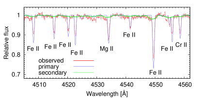
Figure 1: A comparison of the observed spectrum with the synthetic ones of the primary and secondary. The latter is reduced by a factor of 0.255

3 Spectroscopy

3.1 Observations and data reduction

Spectroscopic observations of HD 183986 were carried out with two different instruments. We began at the Stará Lesná observatory (G1 pavilion) in July 2014 with a 60cm, f/12.5 Zeiss Cassegrain telescope equipped with a fiber-fed échelle spectrograph eShel (Pribulla et al., 2015). The spectra, consisting of 24 orders, cover the wavelength range from 4 150 to 7 600 Å. The resolving power of the spectrograph is about $R=10\,000$. An Atik 460EX CCD camera, which has a 2749$\times$2199 array chip, 4.54$\mu$m square pixels, a read-out noise of 5.1 e^- and a gain of 0.26e^-/ADU, was used as a detector. From July 2017, we also observed at the Skalnaté Pleso Observatory (SP), using the 1.3m, f/8.36 Nasmyth-Cassegrain telescope, equipped with a fiber-fed échelle spectrograph of MUSICOS design (Baudrand & Bohm, 1992). The spectra were recorded using an Andor iKon-L DZ936N-BV CCD camera with a 2048$\times$2048 array, 13.5$\mu$m square pixels, 2.9e^- read-out noise and a gain close to unity. The spectral range of the instrument is 4 250-7 375 Å (56 échelle orders) with a maximum resolution of $R=38\,000$. Our observations spanned an interval of 2 334 days.

The raw data were reduced using IRAF package tasks, Linux shell scripts, and FORTRAN programs (Pribulla et al., 2015; Garai et al., 2017). In the first stage, master dark and flat-field frames were produced. In the second stage, photometric calibration of the frames was performed using dark and flat-field frames. Bad pixels were cleaned using a bad pixel mask and cosmic hits were removed using the Pych (2004) program. Usually, three consecutive photometrically-calibrated frames were combined to increase the signal-to-noise ratio (SNR) and to clean any remaining cosmics. The échelle order positions were defined by fitting the 6^th order Chebyshev polynomials to a tungsten-lamp and blue LED spectra tracings. In the following stage, scattered light was modeled and subtracted. Aperture spectra were then extracted for both the object and the ThAr lamp frames and the resulting 2D spectra were dispersion solved. The 2D spectra were, lastly, combined into 1D spectra and rectified to the continuum.

3.2 Primary component velocities and its orbit

The RVs were determined using the cross-correlation function (CCF) technique (Griffin, 1967; Simkin, 1974; Tonry & Davis, 1979; Zverko et al., 2007). Except for the Balmer lines, the observed spectrum of the star included a few tens of metallic absorption lines that were largely of central depths $\approx 0.1$ below the continuum. The strongest one was the line of Mg ii $\lambda$ 4481 Å  with a central depth of $\approx 0.45$ in the spectra, with $R$ = 38 000. We used two wavelength regions, namely 4 400–4 640 Å and 4 900–5 470 Å, which contain an absolute majority of the mentioned metallic lines. Due to the luminosity ratio and the high $v\sin i$, which was estimated to be up to 150 km s^-1, the CCFs represent only the primary component and its orbital motion. The synthetic ”template” spectrum used here was computed with $T_{\rm eff}=10\,600$  K and $\log g=3.63$ rotated with $v\sin i=30$ km s^-1, adopted from Zverko et al. (2013). The RVs are listed in Tables 4 and 5 and plotted in Fig. 2.

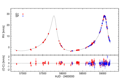
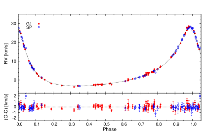
Figure 2: Radial velocities of the primary component of HD 183986 and their best fit and the residuals showing the measurement errors. Radial velocity as a function of time (top) and the corresponding phase diagram (bottom) is shown. Data obtained in the G1 pavilion with the eShel spectrograph (G1), together with those obtained with the MUSICOS at the Skalnaté Pleso observatory (SP), are shown.

Having a sufficient number of spectra for each spectrograph (eShel and MUSICOS), the RV errors were first determined as 1/SNR (see equation 1 of Hatzes et al., 2010). These errors were then re-scaled to give the reduced $\chi^{2}$ = 1 for either of the spectrographs. The scaling constant in $\sigma=C/SNR$ was found to be 28.6 for MUSICOS and 31.4 for eShel. No statistically significant shift of the systemic RV between the spectrographs was found.

All the RVs were modeled simultaneously to obtain the spectroscopic elements. The modeling was performed using a gradient-based optimization (GbO). The best fit to the data showed three deviating points at HJD 2 458 343.51, 2 458 347.38 and 2 458 358.45, which were omitted, and the RVs were re-analyzed. The resulting orbital parameters for the primary component are listed in Table 2, and the best fit with corresponding residuals in Fig. 2. The mean standard deviation of a single RV measurement is about 0.36 km s^-1. This is comparable to the systematic uncertainties caused by the limited stability of the spectrographs. Using the zero point difference of the wavelength solution of the preceding and following comparison spectra, the typical RV stability is 0.20 km s^-1, and 0.05 km s^-1 for MUSICOS and eShel spectrographs, respectively.

We also employed an alternative FOTEL code (Hadrava, 1990), which enables either a simultaneous or a separate analysis of the light curve and radial velocity of a binary star. It is based on the minimization of the sum $\Sigma(O-C)^{2}$ as a function of the orbital elements. The orbital elements of the primary component’s orbit, obtained with the same RV data as in the GbO modelling, are listed in the last column of Table 2. The resulting parameters are mostly within errors of the GbO results.

Table 2: Spectroscopic orbit of the primary component obtained fitting radial velocities from the CCF method. The standard error of the last decimal place is given in parenthesis.

Element		GbO	FOTEL
$P$	[days]	1 268.2(11)	1 267.8(12)
$e$		0.572 8(20)	0.571 4(22)
$\omega$	[rad]	0.354(6)	0.359(7)
$T_{0}$	[HJD]	2 456 528.2(24)	2 456 529.4(27)
$V_{0}$	[km s-1]	4.115(32)	4.030(40)
$K_{1}$	[km s-1]	15.79(5)	15.83(7)
$a_{1}\sin i$	[a.u.]	1.509(5)	1.514(7)
$f(m)$	[M⊙]	0.286(3)	0.288(4)
$\chi^{2}$		147.64	-
d.o.f.		148-6	-
$\Sigma(O-C)^{2}$			0.0660

3.3 Signatures of the secondary component

Zverko et al. (2013) demonstrated that the observed line profiles of the Ca ii $\lambda$ 3933 Å and Mg ii $\lambda$ 4481 Å lines of HD 183986 can be reproduced by superimposing the spectra of two stars, namely a B9.5III and a middle A-type star. They also estimated the flux ratio of the components as $F_{1}/F_{2}$ = 0.9/0.1 in the ultraviolet region and $F_{1}/F_{2}$ = 0.89/0.11 in the blue region.

Now, having the orbital cycle sufficiently covered by the RV observations, we can illustrate how, for example, the profile of the line of Mg ii $\lambda$ 4481 Å varies due to the orbital motion. The spectral lines of the secondary component were recognized by a careful inspection of the spectrum. They are very weak due to the luminosity ratio of the component stars, and in addition, the lines are broadened due to the high projected rotational velocity, $v\sin i$, which may reach up to $\approx$ 150 km s^-1.

Spectra selected close to the extremes of the RV curve, as well as near the systemic velocity, are plotted in Fig. 3. It is well documented that, when the secondary component approaches, a depression in the short-wavelength wing of the line appears while, when it recedes, depression occurs in the red wing of the line. A similar depression in the opposite wings of the line can be clearly seen in the line of the Fe ii $\lambda$ 4549 Å (Fig. 4). The line is, in terms of strength, the second following the line of magnesium Mg ii $\lambda$ 4481 Å. The theoretical spectrum shown here was computed assuming the atmospheric parameters adopted from Zverko et al. (2013), namely $T_{\rm eff}=10\,600$ K, $\log g=3.63$ for the primary and $T_{\rm eff}=8\,200$  K, $\log g=4.2$ for the secondary, and taking into account the ratio of luminosities of the components.

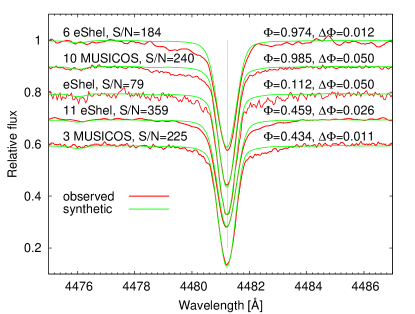
Figure 3: The profile of the Mg ii $\lambda$ 4481 Å near the maximum RV of the primary component (upper 2 spectra), close to the systemic velocity (middle), and the minimum RV (lower 2 spectra). The labels on the left mean that 6, 10, 11 and 3 individual spectra have been co-added to increase the SNR. The corresponding mean phase, $\Phi$, and the phase interval, $\Delta\Phi$, are shown on the right.

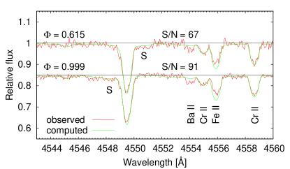
Figure 4: Similar to Fig. 3, but in the vicinity of the Fe ii line $\lambda$ 4549 Å. The computed spectrum is a theoretical one summed from the spectra of the primary and secondary components. The letter ”S” marks the position of the secondary component line.

Table 3: Spectroscopic SB2 orbit obtained by the Fourier disentangling. The standard error of the last decimal place is given in parenthesis. KOREL does not calculate errors of parameters. The errors of $V_{0},K_{1},K_{2},a_{1,2}\sin i,M_{1,2}\sin^{3}i$ and $\Sigma(O-C)^{2}$ are from FOTEL

Parameter
$P$	[days]	1268.2
$e$		0.5729
$\omega$	[rad]	0.359
$T_{0}$	[HJD]	2 456 528.2
$V_{0}$	[km s-1]	4.03(4)
$K_{1}$	[km s-1]	15.82(5)
$K_{2}$	[km s-1]	24.15(5)
$a_{1}\sin i$	[a.u.]	1.514 4
$a_{2}\sin i$	[a.u.]	2.247 5
$M_{1}\sin^{3}i$	[M⊙]	2.93
$M_{2}\sin^{3}i$	[M⊙]	1.92
$q$		0.655
$\Sigma(O-C)^{\rm 2}$		0.138 1

Table 4: Heliocentric radial velocities of HD 183986 from G1. The estimated SNRs at 4400 Å  are also listed.

HJD	RV		SNR	HJD	RV		SNR	HJD	RV	SNR
2 400 000+	[km s-1]			2 400 000+	[km s-1]			2 400 000+	[km s-1]
56845.4475	-2.95	132	58231.6029	-3.27	82	58769.2555	4.30	55
57191.5324	-1.93	126	58344.3883	-2.73	132	58770.2446	3.96	105
57198.4525	-1.77	86	58347.3794	-2.50	134	58771.2281	4.42	99
57207.4420	-2.47	128	58358.3795	-2.92	106	58781.2150	4.05	94
57327.2816	-0.35	87	58361.3937	-2.41	107	58782.2516	4.71	74
57328.3314	0.51	40	58374.3454	-2.39	109	58783.2421	5.04	82
57330.3210	-0.12	53	58378.3288	-2.46	98	58787.2984	5.75	59
57499.5912	4.18	98	58380.3630	-2.48	105	58788.2476	5.43	70
57514.5199	4.24	94	58392.3203	-2.38	94	58924.6172	13.48	32
57516.5285	4.90	138	58405.2533	-2.81	123	58940.5006	14.33	48
57541.5202	5.87	116	58406.2512	-2.20	100	58978.3835	19.50	58
57561.5570	6.71	144	58407.2656	-2.24	108	59011.4915	24.48	53
57564.5105	7.29	101	58576.5496	-0.57	62	59014.3394	25.14	81
57641.3648	11.93	119	58599.5643	0.10	92	59024.3419	26.42	73
57642.3621	12.36	116	58629.5304	0.57	75	59025.4075	28.00	83
57643.3026	12.09	104	58707.3115	1.72	115	59026.4321	27.53	90
57845.5650	16.36	77	58714.3568	2.14	73	59032.3348	27.70	54
57906.5262	5.72	62	58715.3577	2.61	91	59038.3680	28.65	52
57929.5448	3.68	93	58725.3420	2.56	84	59040.4144	28.46	70
57934.5240	3.16	56	58726.4111	2.70	71	59041.4208	27.95	91
57944.4365	2.07	126	58727.3460	3.75	98	59044.4157	27.90	63
57964.4208	1.43	90	58728.3038	3.08	63	59074.3292	26.32	83
57966.4706	0.91	98	58730.3559	2.53	74	59083.2849	24.82	79
57968.4001	1.18	93	58739.2977	3.80	91	59101.2839	19.23	62
57989.4201	0.14	116	58741.2609	3.87	59	59108.2470	18.23	99
58036.2989	-1.89	84	58742.2569	2.73	59	59114.2379	16.50	95
58202.6364	-3.73	98	58745.2722	3.50	62	59141.1980	10.18	70
58229.6100	-3.08	116	58749.2397	3.86	98	59161.2816	7.64	104

Table 5: Heliocentric radial velocities of HD 183986 from SP. Three systematically deviating points, 2 458 343.50870, 2 458 347.38010 and 2 458 358.44960, were not used for the next analysis. The estimated SNRs at 4400 Å  are also listed.

HJD	RV		SNR	HJD	RV		SNR	HJD	RV	SNR
2 400 000+	[km s-1]			2 400 000+	[km s-1]			2 400 000+	[km s-1]
57966.3834	1.38	144	58942.5265	15.10	59	59075.4500	25.50	89
58236.5091	-3.13	69	58946.5072	15.73	89	59087.3447	22.93	84
58245.5391	-3.32	79	58959.5131	16.88	36	59089.4625	22.80	45
58343.5087	-4.65	83	58962.4249	17.92	59	59090.3030	22.06	92
58347.3801	-4.33	112	58987.4497	21.18	59	59096.3852	20.76	88
58358.4496	-4.65	88	58988.4476	21.40	76	59105.3386	18.32	93
58575.4717	-0.72	67	58991.4351	21.85	40	59106.2910	18.43	73
58644.4567	0.60	109	59004.4100	23.98	67	59107.3438	17.76	95
58650.4295	0.85	96	59007.3186	23.58	75	59108.3786	17.52	119
58676.4817	1.38	51	59028.4739	27.19	79	59120.2311	16.90	70
58679.4284	1.37	41	59029.4058	27.12	75	59146.2498	9.46	86
58680.3978	1.65	86	59031.3720	27.32	50	59150.2405	8.81	57
58705.4143	2.10	67	59036.4256	27.83	106	59151.2793	8.70	69
58721.4782	2.19	92	59038.4410	27.78	62	59154.2333	8.29	63
58723.4627	2.48	79	59045.3634	28.39	73	59163.2130	6.80	98
58782.2594	4.68	71	59050.4923	28.41	72	59165.3082	6.74	86
58783.2614	4.66	91	59059.3083	26.94	52	59166.1999	6.47	63
58784.2637	4.86	66	59060.3910	27.56	89	59167.2362	6.61	54
58795.2202	3.97	51	59061.4166	27.55	85	59175.1781	5.85	93
58811.1984	5.59	76	59062.3655	27.39	64	59178.2052	5.11	79
58917.6143	12.76	83	59063.3634	27.39	91	59180.2369	5.82	62
58926.5886	13.50	83	59067.4542	27.62	99	.	.	.
58928.5464	13.68	78	59074.3237	25.83	90	.	.	.

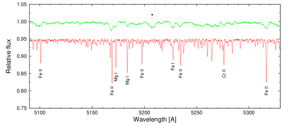
Figure 5: The disentangled spectra in the yellow region normalised to unity. Some of the spectral lines identified in the spectrum of the primary component (lower spectrum) are also identifiable as rotationally-widened in the spectrum of the cooler secondary component (upper spectrum). A remaining artifact depression, resulting from the disentangling, is visible in the secondary-spectrum (black triangle). The primary component spectrum was shifted for clarity by $-$0.05.

3.4 Disentangling spectra with KOREL

Spectral disentangling is a powerful method used to separate component spectra of spectroscopic binaries (SB2) and multiple systems. There are several viable approaches, e.g. disentangling in the wavelength domain (Simon & Sturm, 1994; Ilijic, 2004), Fourier disentangling (Hadrava, 1995), or tomographic decomposition (Bagnuolo & Gies, 1991; Konacki et al., 2010). Each of these techniques has different assumptions. While some of them require knowledge of radial velocities, or of basic orbital parameters, others provide results with a complete solution without RVs as an input. Nevertheless, spectral disentangling is the method of choice for high-contrast systems. The disentangling typically provides spectra of the fainter components with a higher SNR, which can be used for spectroscopic analysis. The advantages and limitations of the above techniques are discussed in detail by e.g., Ilijic (2004) or Hełminiak et al. (2019).

In order to separate the component spectra of HD 183986, the Fourier disentangling method of Hadrava (1995) was used. KOREL (Hadrava, 2004) is a code for decomposition of component spectra and determination of the orbital elements of binary and multiple stars by means of Fourier disentangling. It is especially suitable for spectra with faint spectral lines of the secondary component superimposed on strong lines of primary ones. It enables multiple spectral regions to be analyzed simultaneously in a set of spectra.

We selected 23 out of 67 MUSICOS (SP) spectra, 15 of them with SNR$\mathrel{\mathchoice{\vbox{\offinterlineskip\halign{\hfil$\displaystyle#$\hfil\cr>\cr\vskip 1.2pt\cr=\cr}}}{\vbox{\offinterlineskip\halign{\hfil$\textstyle#$\hfil\cr>\cr\vskip 1.2pt\cr=\cr}}}{\vbox{\offinterlineskip\halign{\hfil$\scriptstyle#$\hfil\cr>\cr\vskip 1.0pt\cr=\cr}}}{\vbox{\offinterlineskip\halign{\hfil$\scriptscriptstyle#$\hfil\cr>\cr\vskip 0.9pt\cr=\cr}}}}89$; a further 8 with SNR$\mathrel{\mathchoice{\vbox{\offinterlineskip\halign{\hfil$\displaystyle#$\hfil\cr>\cr\vskip 1.2pt\cr=\cr}}}{\vbox{\offinterlineskip\halign{\hfil$\textstyle#$\hfil\cr>\cr\vskip 1.2pt\cr=\cr}}}{\vbox{\offinterlineskip\halign{\hfil$\scriptstyle#$\hfil\cr>\cr\vskip 1.0pt\cr=\cr}}}{\vbox{\offinterlineskip\halign{\hfil$\scriptscriptstyle#$\hfil\cr>\cr\vskip 0.9pt\cr=\cr}}}}62$ were added for a better covering of the orbital phase. Two sections well populated with metallic lines were selected, namely from 4 377–4 650 Å and 5 031–5 359 Å, avoiding the region of the $H_{\beta}$ line, where the continuum position is often uncertain. The wavelength scale was converted to the RV scale with a constant step of 4.3 km s^-1, thus giving 4 096 = $2^{12}$ frequency points.

Having an initial set of orbital elements, the code enables each parameter, individually, to be adjusted while the others are kept fixed. Furthermore, all six elements can be adjusted simultaneously. Various combinations of fixed and adjusted elements are also possible.

We adopted the elements corresponding to the orbit of the primary component that were derived using both the eShel and MUSICOS data as they together span over 2 334 days, while the MUSICOS data used in KOREL covers only 1 214 days, which is slightly lower than the orbital period.

First, we fixed the orbital period and the time of the periastron passage, and the eccentricity was adjusted while keeping the remaining elements fixed. We then adjusted the argument of periastron $\omega$, the semi-amplitude $K_{1}$, and the mass ratio $q=M_{2}/M_{1}$ with the new values of the preceding elements fixed. Next, those four elements were converged simultaneously. And lastly, all the 6 elements were converged simultaneously. The resulting parameter set is given in Table 3. The disentangled spectra are plotted in Fig. 5. In the case of the secondary component, some artifacts very probably resulting from the disentangling are visible.

4 Spectra modeling

The KOREL disentangling does not provide the flux ratio of the components (see e.g., Pavlovski & Hensberge, 2010; Lehmann & Tkachenko, 2012). Hence, prior to further modeling, the component spectra must be corrected for the contribution of the other component. We can estimate the flux ratio from the observed color of the system and the mass ratio determined by the disentangling. Applying the programs UVBYBETA (Moon & Dworetsky, 1985) and TEFFLOG (Moon & Dworetsky, 1985), using the $uvby\beta$ indices of HD 183986 (Wenger et al., 2000), we get $T_{\rm eff}=10\,490$ K. As initial values, we used the data summarized in the Astrophysical Quantities (TAQ) (Cox, 2000). This temperature corresponds to a B9.5V star with $M_{1}=3.1$ M_☉ and $R_{1}$ = 2.70 R_☉. Adopting the KOREL mass ratio, $q=0.655$, the secondary mass is about $M_{2}=2.0$ M_☉. This corresponds to an A5V star with about $R_{2}$ = 1.70 R_☉. Now we can estimate the flux ratio of the components in both the blue and yellow regions. In Tab. 15.8 of TAQ, we estimate B9.5V, $M(V)=0.425$ mag for the primary, and with a corresponding $B-V=-0.045$ mag, we get $M(B)=0.380$ mag. For the secondary A5V, there is $M(V)=1.95$ mag, $B-V=0.15$ mag, and $M(B)=2.10$ mag. Using $M(B)_{\rm prim}-M(B)_{\rm sec}=-2.5\times\log(F_{1}/F_{2})$, we arrive at a flux ratio of $F_{2}/F_{1}=0.17/0.83$ = 0.205 in the $B$ band. For the $V$ band, we get $F_{2}/F_{1}=0.20/0.80$ = 0.245.

The component spectra were modeled to determine the atmospheric parameters $T_{\rm eff}$, $\log g$, metallicity, and the projected rotational velocity, $v\sin i$. We used code iSpec (Blanco-Cuaresma et al., 2014; Blanco-Cuaresma, 2019) based on the SPECTRUM (Gray & Corbally, 1994). Prior to the modeling, the line depth of either component was corrected (increased) to take into account the contribution of the other component. The (continuum) flux ratios estimated above were taken into account.

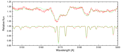
Figure 6: Disentangled spectra of the components (red lines) and their best fits with synthetic spectra obtained from iSpec. The line depth of the components was corrected for the contribution of the other component. The spectrum of the secondary was shifted by +0.2 for clarity

The resulting parameters for the primary component in the blue section (4393 - 4639 Å) of the spectrum are $T_{\rm eff}$ = 11 000$\pm$500 K, $\log g$ = 4.17$\pm$0.45, [M/H] = 0.19$\pm$0.18, and $v\sin i$ = 27.9$\pm$2.5 km s^-1. An attempt to adjust the individual abundances of the elements did not lead to a significant improvement in the fit. The yellow section of the spectrum (5034 - 5333 Å) resulted in a consistent parameter set: $T_{\rm eff}$ = 11 000$\pm$400 K, $\log g$ = 4.37$\pm$0.60, [M/H] = 0.35$\pm$0.08, and $v\sin i$ = 29.1 $\pm$ 3.2 km s^-1. The surface gravity is consistent with the main-sequence evolutionary status. A segment of the yellow part of the spectrum is plotted in Fig. 6.

Modeling the secondary component spectrum was difficult and the results are much less robust. A comparison of the disentangled spectrum of the secondary component with the synthetic spectra showed that numerous dips cannot be identified with the spectral lines but are artifacts resulting from an incorrect continuum definition. The artifacts are much less numerous in the yellow region (see Fig. 5). To arrive at a useful fit, the continuum artifacts were skipped. Thus, in the yellow spectrum, the analysis used the three least-affected segments: 5032 - 5200 Å, 5213 - 5241 Å, and 5259 - 5332 Å. To avoid non-physical parameters (e.g. zero surface gravity), only the surface temperature and the projected rotational velocity were adjusted, fixing $\log g$ = 4.2 and [M/H] = 0 (solar metallicity). This resulted in $T_{\rm eff}$ = 8 420$\pm$130 K and $v\sin i$ = 134 $\pm$ 10 km s^-1. The blue section (segments 4440 - 4496 Å, and 4513 - 4589 Å) was modeled under the same assumptions, resulting in $T_{\rm eff}$ = 7 780$\pm$140 K and $v\sin i$ = 121 $\pm$7 km s^-1. We also attempted to determine the parameters from the two segments in the blue part separately. While the resulting rotational velocities are similar, $v\sin i$ = 124 $\pm$9 km s^-1 and $v\sin i$ = 118$\pm$11 km s^-1, the temperatures differ by almost 600 K. Due to the numerous artifacts in the secondary component’s spectrum in the blue region, we prefer the parameters obtained from the yellow part of the spectrum.

The iSpec code searches for the optimal parameters, using the Levenberg-Marquard algorithm, and the errors are estimated from the co-variance matrix (see Blanco-Cuaresma et al., 2014). The errors strongly depend on the supplied uncertainties of the data. The error estimates should also be taken with caution because of the problematic continuum normalization (especially of the secondary component). A more reliable parameter estimate would require data with a better spectrophotometric calibration and higher spectral resolution.

5 TESS Photometry

In this study, we also analyzed the photometric data acquired by the Transiting Exoplanet Survey Satellite (TESS), which is open to public access. The satellite, launched in 2018, was designed as an all-sky space survey searching for exoplanets orbiting stars brighter than 12 mag (Ricker et al., 2014). The spacecraft consists of four 100-mm telescopes (f/1.4) with four CCD cameras, each with a 4 Mpix chip. The combined field of view is 24 $\times$ 96 degrees. TESS uses the broad bandpass filter (600 – 1000 nm), which is centered on the I_C filter. During the primary mission (from July 2018 to July 2020), nearly the whole sky was observed in 26 sectors. Each sector is 27.4 days long. Every 30 minutes, the full-frame image (FFI) was obtained. For selected targets, the short-cadence (SC) data are available. They are collected every 2 minutes. In July 2020, the mission was extended for the following two years and slightly modified. The FFI are obtained every 10 minutes (Bell, 2020), and the number of targets with SC data was increased and, for very interesting targets, the data cadence, as short as 20 seconds, was also collected.

HD 183986 was observed by TESS in Sector 14 from July 18 to August 15, 2019. However, only FFIs are available. Their cadence (30 minutes) is not sufficient for precise period analysis and produces many spurious low-amplitude frequencies. During the extended mission, this target was observed in two consecutive sectors (Sector 40 and 41), from June 24 to August 20, 2021. SC data are also available from these sectors. A further period analysis was primarily based on the SC data and the FFIs (with improved 10-minute cadence) serve for confirmation of our results. We used an open-source package, eleanor (Feinstein et al., 2019) to obtain a light curve from TESS FFIs. This package cuts a small area (20 $\times$ 20 pixels, i.e. 7 $\times$ 7 arcmin) around the target and downloads only this part of the FFIs. In the next stage, it automatically selects the optimal shape and size of the aperture. The remaining part of the image cut is used to model the background. This workflow, and the quality of the final light curve, is very similar to the PDCSAP_FLUX data of TESS SC data. Finally, the brightness of the star was transformed from fluxes to TESS magnitudes.

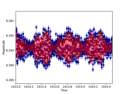
Figure 7: Part of light curve of HD 183986 obtained by TESS in SC mode, together with a model from period analysis. Time is given as BJD - 2 457 000.

A small part of the light curve of HD 183986 obtained from TESS is shown in Fig. 7. No long-term changes of the light curve could be observed as the observations span a period of about 57 days. The pulsations with beats are clearly visible. The period of the beats is about 9.5 hours. The scatter of data caused by the beats is about 1 mmag around the mean value. The amplitudes of the individual pulsation modes is less than 0.5 mmag. The mean uncertainty of the data points is about 0.15 mmag. No significant change of brightness between the years 2019 (Sector 14) and 2021 (Sectors 40 and 41) was observed.

5.1 Period analysis

Table 6: Short-periodic signals found in the TESS data – frequencies, periods and amplitudes of associated sine waves. FAP - false alarm probability.

Frequency	Period	Amplitude	FAP
(d-1)	(min)	(mmag)	(%)
35.80140 $\pm$ 0.00008	40.2219 $\pm$ 0.0001	0.4670 $\pm$ 0.0026	$<10^{-322}$
38.18852 $\pm$ 0.00009	37.7077 $\pm$ 0.0001	0.3154 $\pm$ 0.0020	$<10^{-322}$
29.86847 $\pm$ 0.00016	48.2114 $\pm$ 0.0003	0.1632 $\pm$ 0.0019	$<10^{-322}$
32.26096 $\pm$ 0.00022	44.6360 $\pm$ 0.0003	0.1083 $\pm$ 0.0018	$<10^{-322}$
33.99184 $\pm$ 0.00025	42.3631 $\pm$ 0.0003	0.0905 $\pm$ 0.0017	$<10^{-322}$
36.03922 $\pm$ 0.00035	39.9565 $\pm$ 0.0004	0.0668 $\pm$ 0.0017	$<10^{-322}$
26.76969 $\pm$ 0.00040	53.7922 $\pm$ 0.0008	0.0576 $\pm$ 0.0017	$10^{-255}$
36.18048 $\pm$ 0.00057	39.8005 $\pm$ 0.0006	0.0416 $\pm$ 0.0016	$10^{-134}$
35.10046 $\pm$ 0.00055	41.0251 $\pm$ 0.0006	0.0403 $\pm$ 0.0016	$10^{-119}$
38.20103 $\pm$ 0.00050	37.6953 $\pm$ 0.0005	0.0358 $\pm$ 0.0016	$10^{-100}$
27.10228 $\pm$ 0.00064	53.1321 $\pm$ 0.0013	0.0344 $\pm$ 0.0016	$10^{-94}$
35.78888 $\pm$ 0.00058	40.2360 $\pm$ 0.0006	0.0317 $\pm$ 0.0016	$10^{-80}$
38.17779 $\pm$ 0.00083	37.7183 $\pm$ 0.0008	0.0248 $\pm$ 0.0016	$10^{-47}$
34.13131 $\pm$ 0.00088	42.1900 $\pm$ 0.0011	0.0239 $\pm$ 0.0016	$10^{-43}$
35.81213 $\pm$ 0.00098	40.2098 $\pm$ 0.0011	0.0217 $\pm$ 0.0016	$10^{-35}$
38.54971 $\pm$ 0.00116	37.3544 $\pm$ 0.0011	0.0213 $\pm$ 0.0016	$10^{-34}$
47.20413 $\pm$ 0.00116	30.5058 $\pm$ 0.0007	0.0194 $\pm$ 0.0016	$10^{-27}$
27.17201 $\pm$ 0.00114	52.9957 $\pm$ 0.0022	0.0189 $\pm$ 0.0016	$10^{-26}$
31.38478 $\pm$ 0.00127	45.8821 $\pm$ 0.0019	0.0176 $\pm$ 0.0016	$10^{-21}$
33.96859 $\pm$ 0.00124	42.3921 $\pm$ 0.0016	0.0154 $\pm$ 0.0016	$10^{-15}$
40.98869 $\pm$ 0.00146	35.1317 $\pm$ 0.0013	0.0142 $\pm$ 0.0016	$10^{-12}$
43.37044 $\pm$ 0.00183	33.2023 $\pm$ 0.0014	0.0129 $\pm$ 0.0016	$10^{-9}$
35.52424 $\pm$ 0.00170	40.5357 $\pm$ 0.0019	0.0124 $\pm$ 0.0016	$10^{-8}$
40.96186 $\pm$ 0.00201	35.1546 $\pm$ 0.0017	0.0122 $\pm$ 0.0016	$10^{-7}$
27.96951 $\pm$ 0.00179	51.4846 $\pm$ 0.0033	0.0120 $\pm$ 0.0016	$10^{-7}$
73.98813 $\pm$ 0.00173	19.4626 $\pm$ 0.0005	0.0119 $\pm$ 0.0016	$10^{-7}$
27.66911 $\pm$ 0.00190	52.0436 $\pm$ 0.0036	0.0119 $\pm$ 0.0016	$10^{-7}$
37.12996 $\pm$ 0.00207	38.7827 $\pm$ 0.0022	0.0116 $\pm$ 0.0016	$10^{-6}$
34.47284 $\pm$ 0.00224	41.7720 $\pm$ 0.0027	0.0110 $\pm$ 0.0015	$10^{-5}$
38.24037 $\pm$ 0.00211	37.6565 $\pm$ 0.0021	0.0107 $\pm$ 0.0015	$10^{-4}$
38.47998 $\pm$ 0.00241	37.4221 $\pm$ 0.0023	0.0102 $\pm$ 0.0015	$10^{-4}$
37.41784 $\pm$ 0.00227	38.4843 $\pm$ 0.0023	0.0093 $\pm$ 0.0015	0.019
26.38882 $\pm$ 0.00213	54.5686 $\pm$ 0.0044	0.0093 $\pm$ 0.0015	0.020
45.60557 $\pm$ 0.00246	31.5751 $\pm$ 0.0017	0.0090 $\pm$ 0.0015	0.069

Table 7: Long-periodic signals found in the TESS data. For description, see Tab. 6.

Frequency	Period	Amplitude	FAP
(d-1)	(d)	(mmag)	(%)
0.17702 $\pm$ 0.00178	5.6490 $\pm$ 0.0569	0.0163 $\pm$ 0.0016	$10^{-18}$
0.10729 $\pm$ 0.00166	9.3208 $\pm$ 0.1445	0.0141 $\pm$ 0.0016	$10^{-11}$
0.23067 $\pm$ 0.00168	4.3353 $\pm$ 0.0316	0.0137 $\pm$ 0.0016	$10^{-11}$
1.22664 $\pm$ 0.00195	0.8152 $\pm$ 0.0013	0.0116 $\pm$ 0.0016	$10^{-6}$
0.19133 $\pm$ 0.00197	5.2267 $\pm$ 0.0537	0.0106 $\pm$ 0.0015	$10^{-4}$
0.32543 $\pm$ 0.00217	3.0728 $\pm$ 0.0205	0.0112 $\pm$ 0.0015	$10^{-6}$
0.41663 $\pm$ 0.00249	2.4002 $\pm$ 0.0143	0.0102 $\pm$ 0.0015	$10^{-3}$
1.00849 $\pm$ 0.00324	0.9916 $\pm$ 0.0032	0.0100 $\pm$ 0.0015	0.001
6.86095 $\pm$ 0.00219	0.1458 $\pm$ 0.0001	0.0098 $\pm$ 0.0015	0.003
0.91730 $\pm$ 0.00214	1.0901 $\pm$ 0.0026	0.0094 $\pm$ 0.0015	0.018
0.99419 $\pm$ 0.00211	1.0058 $\pm$ 0.0022	0.0090 $\pm$ 0.0015	0.079

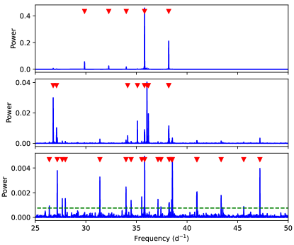
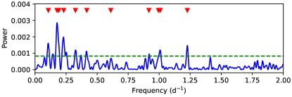
Figure 8: Periodograms associated to the SC data. The dashed horizontal line provides FAP (false alarm probability) levels of 0.3%. The red triangles show the frequencies found, and listed in Tab. 6. Top: high frequencies (periods less than an hour). Bottom: low frequencies (periods more than one day).

The Generalized Lomb-Scargle (GLS; Zechmeister & Kürster, 2009) periodogram was used to find all of the frequencies in the data. At first, we constructed a GLS periodogram from the original data. We identified the highest power peak and subtracted the associated sine wave from the light curve. Next, we generated a GLS periodogram only from the obtained residua. We repeated this procedure until the false-alarm probability (FAP) level of 0.3% was reached. This value corresponds to $3\sigma$-confidence. Using this procedure, we removed all aliases.

We found 45 frequencies (listed in Tab. 6 and 7) with FAP levels less than 0.3%. The amplitudes of periodic signals with a FAP above this limit are significantly smaller than the precision of the input photometric data. Therefore, we assumed that they are only noise. The corresponding periods of the detected signals were in a range from 30 minutes to 5.6 days. Most of them are shorter than one hour. The amplitudes of the associated sine waves were smaller and range from 0.5 mmag to less than 0.01 mmag (for the most powerless frequencies). Periodograms, where all the frequencies are marked, are in Fig. 8. The general shape of the light curve is given by the 5 most significant frequencies with amplitudes larger than approx. 0.1 mmag (top panel of Fig. 8; with periods 40.2, 37.7, 48.2, 44.6 and 42.4 minutes). The reality of some frequencies (mainly those in the third panel of Fig. 8) with small amplitudes and a relatively high FAP is questionable. Their amplitudes are on a level of errors of TESS observations and, therefore, they could only be the result of noise in the light curve. Photometric data with a higher precision, obtained over a longer time interval, are needed to confirm these frequencies. On the other side of our periodograms, we found 11 signals with longer periods (from a few hours to a few days; bottom panel of Fig. 8 and Tab. 7). These frequencies probably result from instrumental effects.

We used photometric data obtained from FFI, with a cumulative exposure time of 10 minutes, to check the results of our period analysis. The main advantage of using this data is that the photometric precision is more than as twice good as the SC data – the mean uncertainty is 0.068 mmag. Their time resolution is also sufficient to distinguish 40-minutes pulsations. The Nyquist frequency is 72 d^-1, with a corresponding period of 20 minutes. We found 36 frequencies with a FAP below our $3\sigma$ level. All the most significant frequencies found using the SC data were confirmed. However, only one of the low frequencies (with a period of 0.8152 days or 19.6 hours) is also present in FFI data. This fact confirms our previous hypothesis that all long-periodic signals are spurious. Moreover, the amplitude of this single long-periodic signal present in both data sets is significantly below the precision of the input data. Therefore, its nature and reality is more than questionable.

5.2 A $\delta$ Scuti pulsations

In general, photometric variations with amplitudes 0.003 to 0.9 mag, with periods of 0.02 d - 0.25 d, in stars within the spectral type range A0 to F5, are typical of $\delta$ Scuti stars (Breger, 2000a). Since the majority of $\delta$ Scuti stars are multi-mode pulsators, the most plausible explanation is that the pulsator could be the secondary component of the binary HD 183986. According to Fernie (1964), the relation between the period and the mass and radius of a radially pulsating star is

$$P=Q\times(M_{\star}/M_{\sun})^{-1/2}\times(R_{\star}/R_{\sun})^{3/2}.$$ (1)

Breger & Bregman (1975) deduced average values $Q=0.033,0.025$ and 0.020 days for the fundamental frequency, its first and second overtones. The values may vary due to, for example, rotation, or differ for hot and cool $\delta$ Scuti-type stars.

With the mass and radius of the secondary estimated in Sec. 4, we get a fundamental frequency of $f_{0}=19.8$  d^-1  and with the values for the primary, we get $f_{0}=12.07$  d^-1. Neither of the frequencies was detected in the TESS photometry. The observed frequencies are, therefore, higher non-radial pulsational modes.

It is important to note that mode identification is more difficult for $\delta$ Scuti stars because they are located at the intersection between the classical instability strip and the main sequence in the HR diagram, a region where the asymptotic theory of non-radial pulsations is invalid due to low-order modes (complicated by avoided crossing and mixed modes). Although there are examples of mode identification based on long-term ground-based observations (e.g. $\tau$ Peg, Kennelly et al. (1998) or 4 CVn, Breger (2000b)), only a few modes have been identified by comparing the observed frequencies with modelling.

Concerning the low-amplitude $\delta$ Scuti stars (LADS), HD 174936 (García Hernández et al., 2009), HD 50844 (Poretti et al., 2009), and HD 50870 (Mantegazza et al., 2012) showed an extremely rich frequency content of low-amplitude peaks in the range 0-35 d^-1 . A similar dense distribution was obtained in KIC 4840675 (Balona et al., 2012a). However, KIC 9700322 (Breger et al., 2011), one of the coolest $\delta$ Scuti stars with $T_{\rm eff}$ = 6 700 K, revealed a remarkably simple frequency content, with only two radial modes and a large number of combination frequencies and rotational modulations. Based on the MOST satellite data, Monnier et al. (2010) identified 57 distinct pulsation modes in $\alpha$ Oph above a stochastic granulation noise.

A good example of a high-amplitude $\delta$ Scuti (HADS) star is V2367 Cyg. Almost all the light variation of V2367 Cyg (Balona et al., 2012b) is attributed to three modes and their combination frequencies. The authors also detected several hundred other frequencies of very low amplitude in the star (with $T_{\rm eff}$ = 7 300 K). On the other hand, twelve independent terms, beside the radial fundamental mode and its harmonics up to the tenth harmonic, were identified in the light of CoRoT 101155310 (Poretti et al., 2011). Regarding the linear combinations of modes, only 61 frequencies were found, down to 0.1 mmag. A much smaller number of low-amplitude modes were thus reported for this HADS star, although it has the same effective temperature as V2367 Cyg. As the examples show, a large number of low-amplitude modes have been detected in both of the largest subgroups of $\delta$ Scuti stars by various space missions.

Although an investigation of the stellar energy balance proved that $\delta$ Scuti stars are energetically and mechanically stable even when hundreds of pulsational modes are present (Moya & Rodríguez-López, 2010), the number of modes can also be interpreted as non-radial pulsation superimposed on granulation noise (Kallinger & Matthews, 2010).

It seems that in HD 183986, we have reached a level of precision where the interpretation of the periodicities arising from different physical processes can be quite difficult. The presence of non-radial modes and granulation noise seem to wash out the physical separation of the LADS and HADS groups. It may be that only the selection mechanism of the excited modes is different in the two groups (Paparó, 2019). However, we do not exactly know the nature of the selection mechanism. Any step towards understanding the selection mechanism of non-radial modes in $\delta$ Scuti stars would, therefore, be very valuable. A meaningful direction would be to find some regularities, if there are any, among the increased number of observed frequencies based on a promising parameter such as the frequency spacings.

6 Evolutionary status of the binary system

An important constraint on the system can be based on stellar evolutionary models. We used a calibration of the Geneva evolutionary models of non-rotating stars by Lejeune & Schaerer (2001). Grids for $Z$ = 0.020 were assumed. We began with an apparent $V$ band magnitude and parallax, which are reliable quantities measured to a very good precision. From them, one can calculate the absolute $V$ band magnitude. Assuming a temperature of the primary of 11 000 K, from iSpec modeling, one can plot the location of the star in the HR diagram. This, in fact, represents an upper limit on the mass and brightness of the primary since we did not take into account the contribution of the secondary star. However, the secondary is much fainter and it will not significantly affect the location of the primary star. Interpolating in the evolutionary tracks, the location of the primary corresponds to a star with a mass of 3.2 $M_{\odot}$ and an age of $220\pm 50$ Myr. Note that the isochrone is almost isothermal in this region so its error is mainly given by the error in the effective temperature of the primary star and is not very sensitive to the brightness or flux dilution due to the secondary star.

Next we exploit the mass ratio of $M_{2}/M_{1}$ = 0.655, obtained from the KOREL disentangling, which is also a reliable quantity, and obtain the mass of the secondary of 2.1 $M_{\odot}$. We again interpolate in the evolutionary tracks to obtain the evolution of such a star. Assuming that both stars have the same age, the intersection of this track with the isochrone of the primary gives us the location of the secondary star in the HR diagram. Once we know the brightness of the secondary star, we subtract its value and correct the location of the primary and iterate the whole procedure again. The final location of both stars, as well as that of the whole binary, is shown in Figure 9. The parameters of the stars are summarized in Table 8. One can see that both stars are located on the main sequence. The masses of the stars from evolutionary models are in good agreement with the masses obtained from the spectroscopic orbit. They indicate that the inclination of the orbit must be close to 90 degrees.

Table 8: Stellar parameters based on evolutionary models.

$T_{1}$ [K]	11000$\pm$ 500
$M_{1}$ [M⊙]	3.1$\pm$ 0.2
$T_{2}$ [K]	8900$\pm$ 200
$M_{2}$ [M⊙]	2.0$\pm$ 0.2
Age [Myr]	220$\pm$ 50
$L_{2}/L$	0.19
$L_{1}/L$	0.81
$L_{2}/L_{1}$	0.23

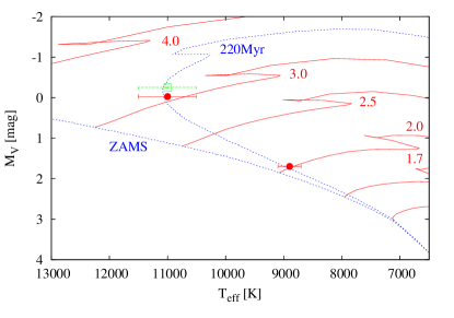
Figure 9: Location of the primary and secondary stars in the HR diagram (full red circles). The location of the whole binary is a green open square. Red full lines are evolutionary tracks of stars with different masses also plotted in red. The two blue dotted lines are isochrones corresponding to ZAMS and 220 Myr.

7 Discussion and conclusions

New and extensive échelle spectroscopy conclusively showed that HD 183986 is a spectroscopic binary and led to the first reliable determination of the orbital period of the system, $P$ = 1268.2$\pm$1.1 days. While the SB1 orbit of the primary component is very robust and well defined, the secondary component is significantly fainter and rotating much faster, which complicates the analysis. The lines of the secondary component were, however, clearly detected in the wings of the strongest metallic lines, e.g. Mg ii $\lambda$ 4481Å , and in the disentangled spectrum.

To arrive at the SB2 orbital parameters, the Fourier domain disentangling using code KOREL was used. The disentangling provided not only the individual component spectra but also the SB2 orbit for the system, including the mass ratio of the components $M_{2}/M_{1}=0.655$. Using the observed color indices, the spectral type of the primary component was estimated as B9.5V. Knowing the mass ratio from the Fourier disentangling indicates an A5V secondary star and the flux ratio in the visual region $F_{2}/F_{1}$ = 0.245. After correcting the spectra for the light contribution of the other component, the disentangled spectra were further modeled to determine the atmospheric parameters, $T_{\rm eff}$, $\log g$, [M/H] and the projected rotational velocity $v\sin i$, using code iSpec. The resulting parameters are consistent with those estimated from the Strömgren $uvby\beta$ color indices. The iSpec modelling proved that the secondary component is a fast rotator.

HD 183986 is an object which, due to the rapid rotation of the secondary component, shows a smaller depth of the spectral lines for its temperature and metallicity from the photometric color indices. Without the inclination angle of the orbit, we cannot reliably determine the absolute parameters of the components. It is, however, highly probable that the next Gaia data release (DR3) in 2022 will provide the visual orbit of the system photocenter and the missing inclination angle required to arrive at the true masses. Without eclipses the component radii cannot be directly determined.

The components of HD 183986 show significantly different projected rotational velocities. The small rotational velocity of the primary, ${v\sin i}$ = 27 km s^-1, and the large rotational velocity of the secondary, ${v\sin i}$ = 120 km s^-1, match perfectly the maxima of the bi-modal distribution of rotational velocities found for normal late-B to mid A-type stars (Royer et al., 2004). The true rotational velocities are, however, unknown and due to the long orbital period of HD 183986, the spin obliquities of the components may be significantly different.

Substantial information on HD 183986 was also obtained from high-precision photometry with the TESS. The satellite provided two month-long and uninterrupted photometry of the object. The data show several signals with periods of about 40 minutes and amplitudes less than 0.5 mmag. Here, we concluded that the observed frequencies are higher non-radial pulsational modes. Also, some lower frequencies (with few-days periods) were found. However, their nature is probably only the result of instrumental effects. A detailed analysis of the observed frequencies is, however, beyond the scope of this paper.

References

- Abt et al. (2002) Abt, H. A., Levato, H., & Grosso, M. 2002, ApJ, 573, 359, doi: 10.1086/340590
- Bagnuolo & Gies (1991) Bagnuolo, W. G., & Gies, D. R. 1991, in Bulletin of the American Astronomical Society, Vol. 23, 1378
- Balona et al. (2012a) Balona, L. A., Breger, M., Catanzaro, G., et al. 2012a, MNRAS, 424, 1187, doi: 10.1111/j.1365-2966.2012.21295.x
- Balona et al. (2012b) Balona, L. A., Lenz, P., Antoci, V., et al. 2012b, MNRAS, 419, 3028, doi: 10.1111/j.1365-2966.2011.19939.x
- Baudrand & Bohm (1992) Baudrand, J., & Bohm, T. 1992, A&A, 259, 711
- Bell (2020) Bell, K. J. 2020, Research Notes of the American Astronomical Society, 4, 19, doi: 10.3847/2515-5172/ab72aa
- Blanco-Cuaresma (2019) Blanco-Cuaresma, S. 2019, MNRAS, 486, 2075, doi: 10.1093/mnras/stz549
- Blanco-Cuaresma et al. (2014) Blanco-Cuaresma, S., Soubiran, C., Heiter, U., & Jofré, P. 2014, A&A, 569, A111, doi: 10.1051/0004-6361/201423945
- Breger (2000a) Breger, M. 2000a, in Astronomical Society of the Pacific Conference Series, Vol. 210, Delta Scuti and Related Stars, ed. M. Breger & M. Montgomery, 3
- Breger (2000b) Breger, M. 2000b, MNRAS, 313, 129, doi: 10.1046/j.1365-8711.2000.03185.x
- Breger & Bregman (1975) Breger, M., & Bregman, J. N. 1975, ApJ, 200, 343, doi: 10.1086/153794
- Breger et al. (2011) Breger, M., Balona, L., Lenz, P., et al. 2011, MNRAS, 414, 1721, doi: 10.1111/j.1365-2966.2011.18508.x
- Cox (2000) Cox, A. N. 2000, Allen’s astrophysical quantities
- Czesla et al. (2019) Czesla, S., Schröter, S., Schneider, C. P., et al. 2019, PyA: Python astronomy-related packages. http://ascl.net/1906.010
- Duquennoy & Mayor (1991) Duquennoy, A., & Mayor, M. 1991, A&A, 500, 337
- ESA (1997) ESA, ed. 1997, ESA Special Publication, Vol. 1200, The HIPPARCOS and TYCHO catalogues. Astrometric and photometric star catalogues derived from the ESA HIPPARCOS Space Astrometry Mission
- Feinstein et al. (2019) Feinstein, A. D., Montet, B. T., Foreman-Mackey, D., et al. 2019, PASP, 131, 094502, doi: 10.1088/1538-3873/ab291c
- Fernie (1964) Fernie, J. D. 1964, ApJ, 140, 1482, doi: 10.1086/148053
- Gaia Collaboration et al. (2018) Gaia Collaboration, Brown, A. G. A., Vallenari, A., et al. 2018, A&A, 616, A1, doi: 10.1051/0004-6361/201833051
- Gaia Collaboration et al. (2021) —. 2021, A&A, 649, A1, doi: 10.1051/0004-6361/202039657
- Garai et al. (2017) Garai, Z., Pribulla, T., Hambálek, Ł., et al. 2017, Astronomische Nachrichten, 338, 35, doi: 10.1002/asna.201613208
- García Hernández et al. (2009) García Hernández, A., Moya, A., Michel, E., et al. 2009, A&A, 506, 79, doi: 10.1051/0004-6361/200911932
- Gray & Corbally (1994) Gray, R. O., & Corbally, C. J. 1994, AJ, 107, 742, doi: 10.1086/116893
- Griffin (1967) Griffin, R. F. 1967, ApJ, 148, 465, doi: 10.1086/149168
- Hadrava (1990) Hadrava, P. 1990, Contributions of the Astronomical Observatory Skalnate Pleso, 20, 23
- Hadrava (1995) —. 1995, A&AS, 114, 393
- Hadrava (2004) —. 2004, Publications of the Astronomical Institute of the Czechoslovak Academy of Sciences, 92, 15
- Hatzes et al. (2010) Hatzes, A. P., Cochran, W. D., & Endl, M. 2010, The Detection of Extrasolar Planets Using Precise Stellar Radial Velocities, ed. N. Haghighipour, Vol. 366, 51, doi: 10.1007/978-90-481-8687-7_3
- Hauck & Mermilliod (1998) Hauck, B., & Mermilliod, M. 1998, A&AS, 129, 431, doi: 10.1051/aas:1998195
- Hełminiak et al. (2019) Hełminiak, K. G., Tokovinin, A., Niemczura, E., et al. 2019, A&A, 622, A114, doi: 10.1051/0004-6361/201732482
- Hoffleit & Warren (1995) Hoffleit, D., & Warren, W. H., J. 1995, VizieR Online Data Catalog, V/50
- Ilijic (2004) Ilijic, S. 2004, in Astronomical Society of the Pacific Conference Series, Vol. 318, Spectroscopically and Spatially Resolving the Components of the Close Binary Stars, ed. R. W. Hilditch, H. Hensberge, & K. Pavlovski, 107–110
- Kallinger & Matthews (2010) Kallinger, T., & Matthews, J. M. 2010, ApJ, 711, L35, doi: 10.1088/2041-8205/711/1/L35
- Kennelly et al. (1998) Kennelly, E. J., Brown, T. M., Kotak, R., et al. 1998, ApJ, 495, 440, doi: 10.1086/305268
- Konacki et al. (2010) Konacki, M., Muterspaugh, M. W., Kulkarni, S. R., & Hełminiak, K. G. 2010, ApJ, 719, 1293, doi: 10.1088/0004-637X/719/2/1293
- Kuiper (1961) Kuiper, G. P. 1961, ApJS, 6, 1, doi: 10.1086/190059
- Latham et al. (2002) Latham, D. W., Stefanik, R. P., Torres, G., et al. 2002, AJ, 124, 1144, doi: 10.1086/341384
- Lehmann & Tkachenko (2012) Lehmann, H., & Tkachenko, A. 2012, in From Interacting Binaries to Exoplanets: Essential Modeling Tools, ed. M. T. Richards & I. Hubeny, Vol. 282, 395–396, doi: 10.1017/S174392131102789X
- Lejeune & Schaerer (2001) Lejeune, T., & Schaerer, D. 2001, A&A, 366, 538, doi: 10.1051/0004-6361:20000214
- Mantegazza et al. (2012) Mantegazza, L., Poretti, E., Michel, E., et al. 2012, A&A, 542, A24, doi: 10.1051/0004-6361/201118682
- Monnier et al. (2010) Monnier, J. D., Townsend, R. H. D., Che, X., et al. 2010, ApJ, 725, 1192, doi: 10.1088/0004-637X/725/1/1192
- Moon & Dworetsky (1985) Moon, T. T., & Dworetsky, M. M. 1985, MNRAS, 217, 305, doi: 10.1093/mnras/217.2.305
- Moya & Rodríguez-López (2010) Moya, A., & Rodríguez-López, C. 2010, ApJ, 710, L7, doi: 10.1088/2041-8205/710/1/L7
- Palmer et al. (1968) Palmer, D. R., Walker, E. N., Jones, D. H. P., & Wallis, R. E. 1968, Royal Greenwich Observatory Bulletins, 135, 385
- Paparó (2019) Paparó, M. 2019, Frontiers in Astronomy and Space Sciences, 6, 26, doi: 10.3389/fspas.2019.00026
- Paunzen (2015) Paunzen, E. 2015, A&A, 580, A23, doi: 10.1051/0004-6361/201526413
- Pavlovski & Hensberge (2010) Pavlovski, K., & Hensberge, H. 2010, in Astronomical Society of the Pacific Conference Series, Vol. 435, Binaries - Key to Comprehension of the Universe, ed. A. Prša & M. Zejda, 207. https://arxiv.org/abs/0909.3246
- Poretti et al. (2009) Poretti, E., Michel, E., Garrido, R., et al. 2009, A&A, 506, 85, doi: 10.1051/0004-6361/200912039
- Poretti et al. (2011) Poretti, E., Rainer, M., Weiss, W. W., et al. 2011, A&A, 528, A147, doi: 10.1051/0004-6361/201016045
- Pribulla et al. (2015) Pribulla, T., Garai, Z., Hambálek, L., et al. 2015, Astronomische Nachrichten, 336, 682, doi: 10.1002/asna.201512202
- Pych (2004) Pych, W. 2004, PASP, 116, 148, doi: 10.1086/381786
- Raghavan et al. (2010) Raghavan, D., McAlister, H. A., Henry, T. J., et al. 2010, ApJS, 190, 1, doi: 10.1088/0067-0049/190/1/1
- Ricker et al. (2014) Ricker, G. R., Winn, J. N., Vanderspek, R., et al. 2014, in Society of Photo-Optical Instrumentation Engineers (SPIE) Conference Series, Vol. 9143, Space Telescopes and Instrumentation 2014: Optical, Infrared, and Millimeter Wave, 914320, doi: 10.1117/12.2063489
- Royer et al. (2004) Royer, F., Zorec, J., & Gómez, A. E. 2004, in The A-Star Puzzle, ed. J. Zverko, J. Ziznovsky, S. J. Adelman, & W. W. Weiss, Vol. 224, 109–114, doi: 10.1017/S1743921304004442
- Simkin (1974) Simkin, S. M. 1974, A&A, 31, 129
- Simon & Sturm (1994) Simon, K. P., & Sturm, E. 1994, A&A, 281, 286
- Skrutskie et al. (2006) Skrutskie, M. F., Cutri, R. M., Stiening, R., et al. 2006, AJ, 131, 1163, doi: 10.1086/498708
- Tody (1986) Tody, D. 1986, in Society of Photo-Optical Instrumentation Engineers (SPIE) Conference Series, Vol. 627, Instrumentation in astronomy VI, ed. D. L. Crawford, 733, doi: 10.1117/12.968154
- Tody (1993) Tody, D. 1993, in Astronomical Society of the Pacific Conference Series, Vol. 52, Astronomical Data Analysis Software and Systems II, ed. R. J. Hanisch, R. J. V. Brissenden, & J. Barnes, 173
- Tonry & Davis (1979) Tonry, J., & Davis, M. 1979, AJ, 84, 1511, doi: 10.1086/112569
- van Leeuwen (2007) van Leeuwen, F. 2007, A&A, 474, 653, doi: 10.1051/0004-6361:20078357
- Vaňko et al. (2020) Vaňko, M., Pribulla, T., Hambálek, Ľ., et al. 2020, Contributions of the Astronomical Observatory Skalnate Pleso, 50, 632, doi: 10.31577/caosp.2020.50.2.632
- Wenger et al. (2000) Wenger, M., Ochsenbein, F., Egret, D., et al. 2000, A&AS, 143, 9, doi: 10.1051/aas:2000332
- Wolff & Preston (1978) Wolff, S. C., & Preston, G. W. 1978, ApJS, 37, 371, doi: 10.1086/190533
- Zechmeister & Kürster (2009) Zechmeister, M., & Kürster, M. 2009, A&A, 496, 577, doi: 10.1051/0004-6361:200811296
- Zverko (2014) Zverko, J. 2014, Contributions of the Astronomical Observatory Skalnate Pleso, 43, 256
- Zverko et al. (2013) Zverko, J., Romanyuk, I., Iliev, I., et al. 2013, Astrophysical Bulletin, 68, 442, doi: 10.1134/S1990341313040056
- Zverko et al. (2011) Zverko, J., Žižňovský, J., Iliev, I., et al. 2011, Astrophysical Bulletin, 66, 325, doi: 10.1134/S1990341311030059
- Zverko et al. (2007) Zverko, J., Žižňovský, J., Mikulášek, Z., & Iliev, I. K. 2007, Contributions of the Astronomical Observatory Skalnate Pleso, 37, 49