Multi-Sample $\zeta$-mixup: Richer, More Realistic Synthetic Samples from a $p$-Series Interpolant

Abstract

Modern deep learning training procedures rely on model regularization techniques such as data augmentation methods, which generate training samples that increase the diversity of data and richness of label information. A popular recent method, mixup, uses convex combinations of pairs of original samples to generate new samples. However, as we show in our experiments, mixup can produce undesirable synthetic samples, where the data is sampled off the manifold and can contain incorrect labels. We propose $\zeta$-mixup, a generalization of mixup with provably and demonstrably desirable properties that allows convex combinations of $N\geq 2$ samples, leading to more realistic and diverse outputs that incorporate information from $N$ original samples by using a $p$-series interpolant. We show that, compared to mixup, $\zeta$-mixup better preserves the intrinsic dimensionality of the original datasets, which is a desirable property for training generalizable models. Furthermore, we show that our implementation of $\zeta$-mixup is faster than mixup, and extensive evaluation on controlled synthetic and 24 real-world natural and medical image classification datasets shows that $\zeta$-mixup outperforms mixup and traditional data augmentation techniques.

1 Introduction

Deep learning-based techniques have demonstrated unprecedented performance improvements over the last decade in a wide range of tasks, including but not limited to image classification, segmentation, and detection, speech recognition, natural language processing, and graph processing [53, 41, 3, 65]. These deep neural networks (DNNs) have a large number of parameters, often in the tens to hundreds of millions, and training accurate, robust, and generalizable models has largely been possible because of large public datasets [19, 43, 18], efficient training methods [52, 57], hardware-accelerated training [58, 10, 49, 13], advances in network architecture design [55, 51, 28], advanced optimizers [21, 70, 36, 20], new regularization layers [56, 34], and other novel regularization techniques. While techniques such as weight decay [40], dropout [56], batch normalization [34], and stochastic depth [32] can be considered as “data independent" regularization schemes [25], popular “data dependent" regularization approaches include data augmentation [42, 12, 39, 71, 55] and adversarial training [24, 6].

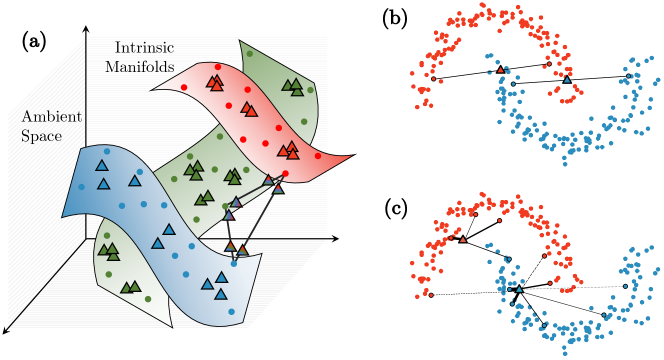
Figure 1: Overview of mixup (b) and $\zeta$-mixup (a, c). The original and synthesized samples are denoted by $\circ$ and $\bigtriangleup$ respectively, and line segments indicate which original samples were used to create the new ones. The line thicknesses denote the relative weights assigned to original samples. Observe how $\zeta$-mixup can mix any number of samples (e.g., 3 in (a) and 4 or 8 in (c)), and that $\zeta$-mixup’s formulation allows the generated samples to be close to the original distribution while still incorporating rich information from several samples.

Given the large parameter space of deep learning models, training on small datasets tends to cause the models to overfit to the training samples. This is especially a problem when training with data from high dimensional input spaces, such as images, because the sampling density is exponentially proportional to $1/\mathcal{D}$, where $\mathcal{D}$ is the dimensionality of the input space [27]. As $\mathcal{D}$ grows larger (typically $10^{4}$ to $10^{6}$ for most real-world image datasets), we need to increase the number of samples exponentially in order to retain the same sampling density. As a result, it is imperative that the training datasets for these models have a sufficiently large number of samples in order to prevent overfitting. Moreover, deep learning models generally exhibit good generalization performance when evaluated on samples that come from a distribution similar to the training samples’ distribution. In addition to their regularization effects to prevent overfitting [30, 29], data augmentation techniques also help the training by synthesizing more samples in order to better learn the training distributions.

Traditional image data augmentation techniques include geometric- and inte-nsity-based transformations, such as affine transformations, rotation, scaling, zooming, cropping, adding noise, etc., and are quite popular in the deep learning literature. For a comprehensive review of data augmentation techniques for deep learning methods on images, we refer the interested readers to the survey by Shorten et al. [54]. In this paper, we focus on a recent and popular data augmentation technique based on a rather simple idea, which generates a convex combination of a pair of input samples, variations of which are presented as mixup [73], Between-Class learning [59], and SamplePairing [33]. The most popular of these approaches, mixup [73], performs data augmentation by generating new training samples from convex combinations of pairs of original samples and linear interpolations of their corresponding labels, leading to new training samples, which are obtained by essentially overlaying 2 images with different transparencies, and new training labels, which are soft probabilistic labels. Other related augmentation methods can broadly be grouped into 3 categories: (a) methods that crop or mask region(s) of the original input image followed by mixup like blending, e.g., CutMix [69] and GridMix [5], (b) methods that generate convex combinations in the learned feature space, e.g., Manifold Mixup [62] and MixFeat [67], and (c) methods that add a learnable component to mixup, e.g., AdaMixUp [25], AutoMix [74], and AutoMix [44]. However, mixup can lead to ghosting artifacts in the synthesized samples (as we show later in the paper, e.g., Fig. 3), in addition to generating synthetic samples with wrong class labels. Moreover, because mixup uses a convex combination of only a pair of points, it can lead to the synthetic samples being generated off the original data manifold (Fig. 1 (a)). This in turn leads to an inflation of the manifold, which can be quantified by an increase in the intrinsic dimensionality of the resulting data distribution, as shown in Fig. 4, which is undesirable since it has been shown that deep models trained on datasets with lower dimensionalities generalize better to unseen samples [48]. Additionally, mixup-like approaches, which crop or mask regions of the input images, may degrade the training data quality by occluding informative and discriminatory regions of images, which is highly undesirable for high-stakes applications such as medical image analysis tasks.

The primary hypothesis of mixup and many of its derivatives is that a model should behave linearly between any two training samples, even if the distance between samples is large. This implies that we may train the model with synthetic samples that have very low confidence of realism; in effect over-regularizing. We instead argue that a model should only behave linearly nearby training samples and that we should thus only generate synthetic examples with high confidence of realism. To achieve this, we propose $\zeta$-mixup, a generalization of mixup with provably desirable properties that addresses the shortcomings of mixup. $\zeta$-mixup generates new training samples by using a convex combination of $N$ samples in a training batch, requires no custom layers or special training procedures to employ, and is faster than mixup in terms of wall-clock time. We show how, as compared to mixup, the $\zeta$-mixup formulation allows for generating more realistic and more diverse samples that better conform to the data manifold (Fig. 1 (b)) with richer labels that incorporate information from multiple classes, and that mixup is indeed a special case of $\zeta$-mixup. We show qualitatively and quantitatively on synthetic and real-world datasets that $\zeta$-mixup’s output better preserves the intrinsic dimensionality of the data than that of mixup. Finally, we demonstrate the efficacy of $\zeta$-mixup on 24 datasets comprising a wide variety of tasks from natural image classification to diagnosis with several medical imaging modalities.

2 Method

Vicinal Risk Minimization: Revisiting the concept of risk minimization from Vapnik [61], given $\mathcal{X}$ and $\mathcal{Y}$ as the input data and the target label distributions respectively, and a family of functions $\mathcal{F}$, the supervised learning setting consists of searching for an optimal function $f\in\mathcal{F}:\mathcal{X}\to\mathcal{Y}$, which minimizes the expected value of a given loss function $\mathcal{L}$ over the data distribution $P(x,y);(x,y)\in(\mathcal{X},\mathcal{Y})$. This expected value of the loss, also known as the expected value of the risk, is given by: $R(f)=\int\mathcal{L}\left(f(x),y\right)\ P(x,y)\ dx\ dy.$ In scenarios when the exact distribution $P(x,y)$ is unknown, such as in practical supervised learning settings with a finite training dataset $\{x_{i},y_{i}\}_{i=1}^{m}$, the common approach is to minimize the risk w.r.t. the empirical data distribution approximated by using delta functions at each sample, $R_{\mathrm{emp}}(f)=\frac{1}{m}\sum_{i=1}^{m}\mathcal{L}\left(f(x_{i}),y_{i}\right),$ and this is known as empirical risk minimization (ERM). However, if the data distribution is smooth, as is the case with most real datasets, it is desirable to minimize the risk in the vicinity of the provided samples [61, 9], $R_{\mathrm{vic}}(f)=\frac{1}{\hat{m}}\sum_{i=1}^{\hat{m}}\mathcal{L}\left(f(\hat{x_{i}}),\hat{y_{i}}\right)$, where $\left\{(\hat{x},\hat{y})\right\}_{i=1}^{\hat{m}}$ are points sampled from the vicinity of the original data distribution, also known as the vicinal distribution $P_{\mathrm{vic}}(x,y)$. This is known as vicinal risk minimization (VRM) and theoretical analysis [61, 9, 72] has shown that VRM generalizes well when at least one of these two criteria are satisfied: (i) the vicinal data distribution $P_{\mathrm{vic}}(x,y)$ must be a good approximation of the actual data distribution $P(x,y)$, and (ii) the class $\mathcal{F}$ of functions must have a suitably small capacity. Since modern deep neural networks have up to hundreds of millions of parameters, it is imperative that the former criteria is met.

Data Augmentation: A popular example of VRM is the use of data augmentation for training deep neural networks. For example, applying geometric and intensity-based transformations to images leads to a diverse training dataset allowing the prediction models to generalize well to unseen samples [54]. However, the assumption of these transformations that points sampled in the vicinity of the original data distribution share the same class label is rather limiting and does not account for complex interactions (e.g., proximity relationships) between class-specific data distributions in the input space. Recent approaches based on convex combinations of pairs of samples to synthesize new training samples aim to alleviate this by allowing the model to learn smoother decision boundaries [62]. Consider the general $\mathcal{K}$-class classification task. mixup [73] synthesizes a new training sample $(\hat{x},\hat{y})$ from training data samples $(x_{i},y_{i})$ and $(x_{j},y_{j})$ as

$$\hat{x}=\lambda x_{i}+(1-\lambda)x_{j};\ \ \hat{y}=\lambda y_{i}+(1-\lambda)y_{j}$$ (1)

where $\lambda\in[0,1]$. The labels $y_{i}$, $y_{j}$ are converted to one-hot encoded vectors to allow for linear interpolation between pairs of labels. However, as we show in our experiments (Sec. 4), mixup leads to the synthesized points being sampled off the data manifold (Fig. 1 (a)).

$\zeta$-mixup Formulation: Going back to the $\mathcal{K}$-class classification task, suppose we are given a set of $N$ points $\{x_{i}\}_{i=1}^{N}$ in a $\mathcal{D}$-dimensional ambient space $\mathbb{R^{\mathcal{D}}}$ with the corresponding labels $\{y_{i}\}_{i=1}^{m}$ in a label space $\mathcal{L}=\{l_{1},\cdots,l_{\mathcal{K}}\}\in\mathbb{R^{\mathcal{K}}}$. Keeping in line with the manifold hypothesis [8, 22], which states that complex data manifolds in high dimensional ambient spaces are actually made up of samples from manifolds with low intrinsic dimensionalities, we assume that the $N$ points are samples from $\mathcal{K}$ manifolds $\{\mathcal{M}_{i}\}_{i=1}^{\mathcal{K}}$ of intrinsic dimensionalities $\{d_{i}\}_{i=1}^{\mathcal{K}}$, where $d_{i}<<D\ \forall i\in[1,\mathcal{K}]$ (Fig. 1 (a)). We seek an augmentation method that facilitates a denser sampling of each intrinsic manifold $\mathcal{M}_{i}$, thus generating more real and more diverse samples with richer labels. Following Wood et al. [64, 63], we consider three criteria for evaluating the quality of synthetic data:

(i) realism: allowing the generation of correctly labeled synthetic samples close to the original samples, ensuring the realism of the synthetic samples,

(ii) diversity: facilitating the generation of more diverse synthetic samples by allowing exploration of the input space, and

(iii) label richness when generating synthetic samples while still staying on the manifold of realistic samples. Additionally, we aim for:

(iv) valid probabilistic labels from combinations of samples along with

(v) computationally efficient (e.g., avoiding inter-sample distance calculations) augmentation of training batches.

To this end, we propose to synthesize a new sample $(x_{k},y_{k})$ as

$$x_{k}=\sum_{i=1}^{N}w_{i}x_{i};\ \ y_{k}=\sum_{i=1}^{N}w_{i}y_{i},$$ (2)

where $w_{i}$s are the weights assigned to the $N$ samples. One such weighting scheme that satisfies the aforementioned requirements consists of sample weights from the terms of a $p$-series, i.e., $w_{i}=i^{-p}$, which is a convergent series for $p\geq 1$. Since this implies that the weight assigned to the first sample will be the largest, we want to randomize the order of the samples to ensure that the synthetic samples are not all generated near one original sample. Therefore, building upon the idea of local synthetic instances initially proposed for the augmentation of connectome dataset [7], we adopt the following formulation: Given $N$ samples (where $2\leq N\leq m$ and thus, theoretically, the entire dataset), an $N\times N$ random permutation matrix $\pi$, and the resulting randomized ordering of samples $s=\pi[1,2,\dots,N]^{T}$, the weights are defined as

$$w_{i}=\frac{s_{i}^{-\gamma}}{C},\ \ i\in[1,N]$$ (3)

where $C$ is the normalization constant and $\gamma$ is a hyperparameter. As we show in our experiments later, $\gamma$ allows us to control how far the synthetic samples can stray away from the original samples. Moreover, in order to ensure that $y_{k}$ in Eqn. 2 is a valid probabilistic label, $w_{i}$ must satisfy $w_{i}\geq 0\ \forall i$ and $\sum_{i=1}^{N}w_{i}=1$. Accordingly, we use $L_{1}$-normalization and $C=\sum_{j=1}^{N}j^{-\gamma}$ is the $N$-truncated Riemann zeta function [50] $\zeta(z)$ evaluated at $z=\gamma$, and call our method $\zeta$-mixup. An illustration of $\zeta$-mixup for $N=3,\mathcal{D}=3,d_{1}=d_{2}=d_{3}=2$ is shown in Fig. 1(a). Notice how despite generating convex combinations of samples from disjoint manifolds, the resulting synthetic samples are close to the original ones. A similar observation can be made for $N=4$ and $N=8$ is shown in Fig. 1(c). Since there exist $N!$ possible $N\times N$ random permutation matrices, given $N$ original samples, $\zeta$-mixup can synthesize $N!$ new samples for a single value of $\gamma$, as compared to mixup which can only synthesize 1 new sample per sample pair for a single value of $\lambda$.

As a result of the aforementioned formulation, $\zeta$-mixup presents two desirable properties that we present in the following 2 theorems (proofs in the Appendix). Theorem 1 states that for all values of $\gamma\geq\gamma_{\mathrm{min}}$, the weight assigned to one sample is greater than the sum of the weights assigned to all the other samples in a batch, thus implicitly introducing the desired notion of linearity in only the locality of the original samples. Theorem 2 states the equivalence of mixup and $\zeta$-mixup and establishes the former as a special case of the latter.

Theorem 1.

For $\gamma\geq\gamma_{\mathrm{min}}=1.72865$, the weight assigned to one sample dominates all other weights, i.e., $\forall\ \gamma\geq 1.72865$, $w_{1}>\sum_{i=2}^{N}w_{i}$.

Theorem 2.

For $N=2$ and $\gamma=\log_{2}\left(\frac{\lambda}{1-\lambda}\right)$, $\zeta$-mixup simplifies to mixup.

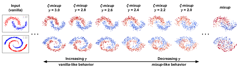
(a) Synthetic two-class 2D data with non-linear class decision boundaries.

(b) Synthetic data distributed along a 3D helical manifold. 2D projections of the 3D manifolds are shown from the following viewpoints top to bottom: (elevation, azimuth): (0°, 0°), (70°, 0°), (90°, 0°). In all the plots, the grey points denote the original input samples.

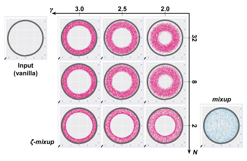
(c) Visualizing the effect of changing $N$ and $\gamma$ on the output of $\zeta$-mixup. 2D projections of the 3D manifolds are shown from the (elevation, azimuth): (0°, 90°) viewpoint.

Figure 2: Visualizing how mixup and $\zeta$-mixup synthesize new samples. Notice that mixup produces samples that (a) are assigned wrong labels and (b) are sampled off the original data manifold, with an extreme example being where the points are sampled from the hollow region in the helix. A moderately low value of $\gamma$ allows for a more reasonable exploration of the data manifold, with higher values of $N$ allowing more diversity in the synthesized points.

3 Datasets and Experimental Details

Synthetic Data: We first generate two-class distributions of $2^{9}=512$ samples with non-linear class boundaries in the shape of interleaving crescents (CRESCENTS) and spirals (SPIRALS), and add Gaussian noise $\mathcal{N}(0,0.1)$, as shown in the “Input" column of Fig. 2 (a). Next, moving on to higher dimensional spaces, we generate synthetic data distributed along a helix. In particular, we sample $2^{13}$ = 8,192 points off a 1-D helix embedded in $\mathbb{R}^{3}$ (see the “Input" column of Fig. 2 (b)) and, as a manifestation of low-D manifolds lying in high-D ambient spaces, a 1-D helix in $\mathbb{R}^{12}$.

Natural Image Datasets (NATURAL): We use MNIST [42], CIFAR-10 and CIFAR-100 [38], Fashion-MNIST (F-MNIST) [66], STL-10 [14], and, to evaluate models on real-world images but with faster training times, two 10-class subsets of the standard ImageNet [19]: Imagenette and Imagewoof [31]. Further details about these datasets and model training are in the Appendix. We train ResNet-18 [28] models and report the overall error rate (ERR) since the datasets have balanced class distributions.

We use 10 skin lesion image diagnosis datasets: ISIC 2016 [26], ISIC 2017 [16], ISIC 2018 [15, 60], MSK [1], (all datasets have dermoscopic images, i.e., captured by a dermatoscope [37, 45], except those denoted by a $\dagger$). We train ResNet-18 and ResNet-50 [28] models on the 5-class diagnosis task used in the literature [35, 17, 2] and report three evaluation metrics that account for the inherent class imbalance: balanced accuracy (i.e., macro-averaged recall) [46] (ACC_bal) and micro- and macro-averaged F1 scores.

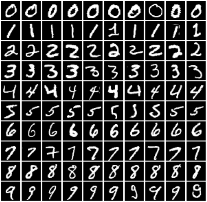
(a) The first 10 images of each MNIST class.

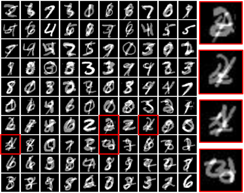
(b) Output of mixup ($N=25$).

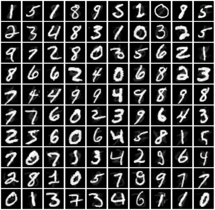
(c) Output of $\zeta$-mixup ($N=25$; $\gamma=2.8$).

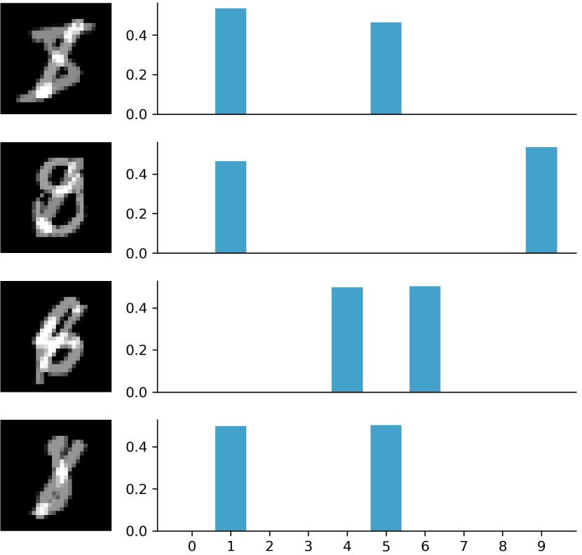
(d) Soft labels of mixup outputs.

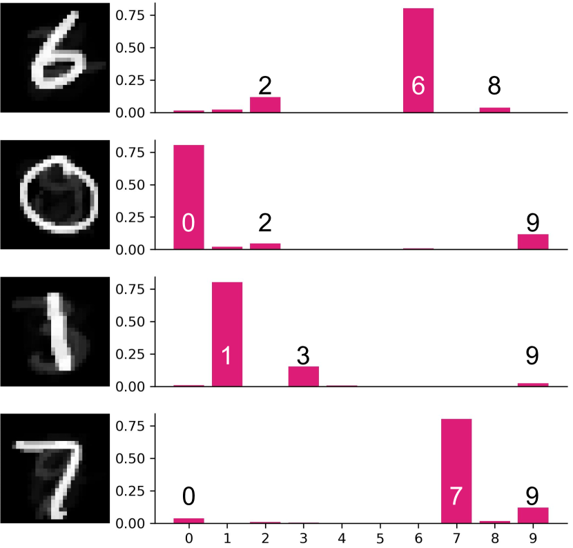
(e) Soft labels of $\zeta$-mixup outputs.

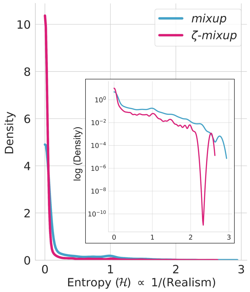
(f) Measuring realism of samples.

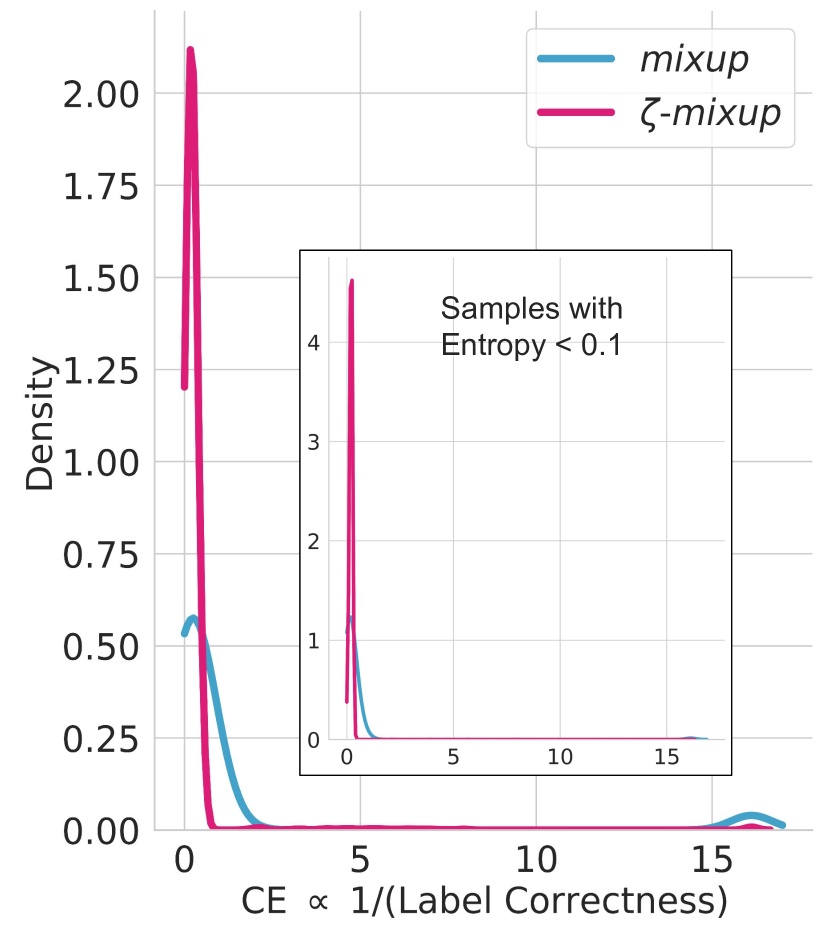
(g) Measuring correctness of labels.

Figure 3: Visualizing the results obtained using mixup and $\zeta$-mixup on images from the MNIST dataset. In (d) and (e), we visualize the probabilistic “soft" labels assigned to images generated by mixup and $\zeta$-mixup respectively. Notice how all images in (d) look close to the digit “8" while their assigned soft labels do not contain the class “8". $\zeta$-mixup alleviates this issue and the soft labels in (e) correspond exactly to the class the synthesized images belong to. Also note how mixup produces images with a wrong label, i.e., a label different from the original labels of the 2 images it is interpolated from. In (f) and (g), we evaluate the realism of mixup’s and $\zeta$-mixup’s generated samples and the correctness of the corresponding labels by measuring the entropy of the Oracle’s predictions ($\mathcal{H}$) and the cross entropy of the Oracle’s predictions with the soft labels (CE) respectively. For both (f) and (g), lower values are better.

Datasets of Other Medical Imaging Modalities (MEDMNIST): To evaluate our models on multiple medical imaging modalities, we use the 8 datasets from the MedMNIST Classification Decathlon [68]: PathMNIST^‡ (histopathology images), DermaMNIST^‡ (multi-source images of pigmented skin lesions), OCTMNIST (optical coherence tomography images), PneumoniaMNIST (pediatric chest X-ray images), BreastMNIST (breast ultrasound images), and OrganMNIST_{A, C, S} (axial, coronal, and sagittal views respectively of 3D computed tomography CT scans). Datasets denoted by $\ddagger$ consist of RGB images, others are grayscale. We train ResNet-18 [28] models and report overall accuracy (ACC) and area under the ROC curve (AUC), similar to the MedMNIST paper [68].

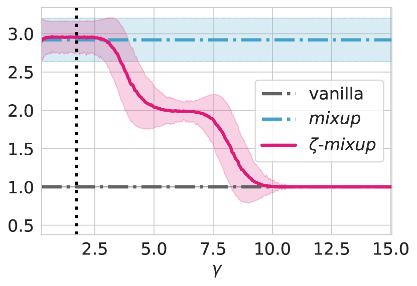
(a) A 1D helix in a 3D embedding space ($n_{\mathrm{NN}}=8$).

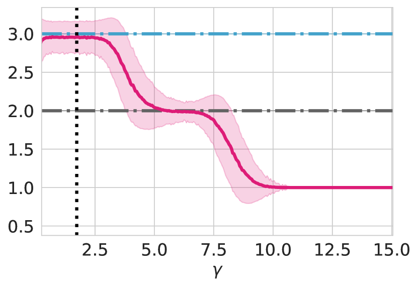
(b) A 1D helix in a 3D embedding space ($n_{\mathrm{NN}}=128$).

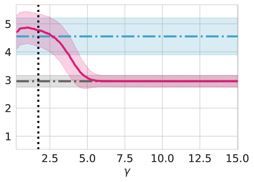
(c) A 3D highly curved manifold in a 12D embedding space ($n_{\mathrm{NN}}=8$).

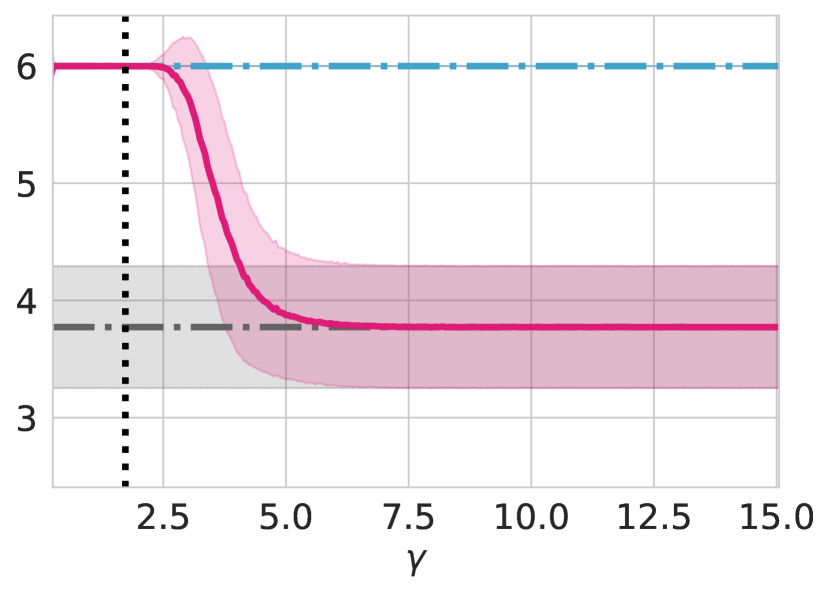
(d) A 3D highly curved manifold in a 12D embedding space ($n_{\mathrm{NN}}=128$).

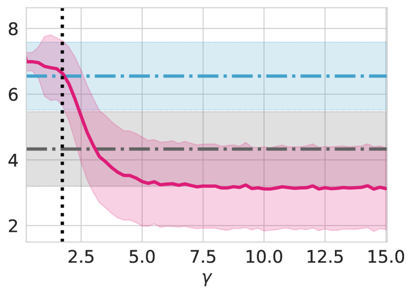
(e) CIFAR-10 images ($n_{\mathrm{NN}}=8$).

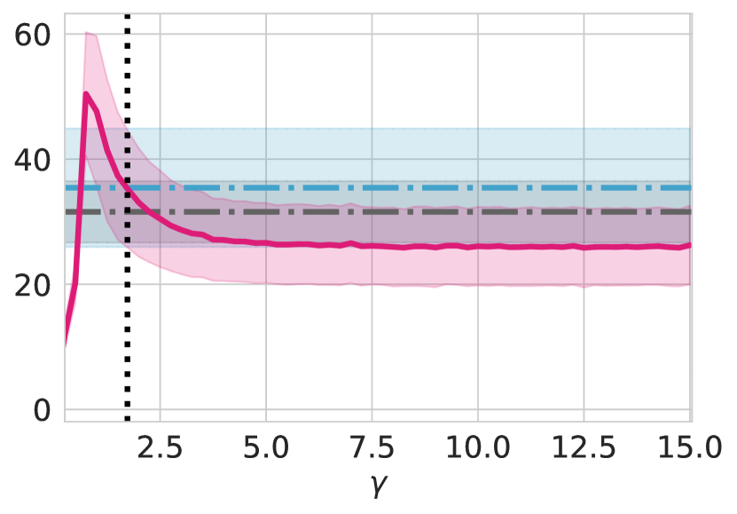
(f) CIFAR-10 images ($n_{\mathrm{NN}}=128$).

(g) CIFAR-100 images ($n_{\mathrm{NN}}=8$).

(h) CIFAR-100 images ($n_{\mathrm{NN}}=128$).

Figure 4: Visualizing how $\zeta$-mixup affects the local intrinsic dimensionality of synthesized datasets distributed as 1D helices ((a) and (b)) and 3D manifold ((c)) in a higher dimensional embedding space as the hyperparameter $\gamma$ changes. The mean and the standard deviation of the intrinsic dimensionality are shown using lines (bold or dashed-dotted) and shaded bands respectively. The vertical dotted line in all the plots denotes the value of $\gamma=\gamma_{\mathrm{min}}$ (Theorem 1).

4 Results and Discussion

We present experimental evaluation on controlled synthetic (1-D manifolds in 2-D and 3-D, 3-D manifolds in 12-D) and on 24 real-world natural and medical image datasets of various modalities. We evaluate the quality of $\zeta$-mixup’s outputs: directly, by assessing the realism, label correctness, diversity, richness [63, 64], and preservation of intrinsic dimensionality of the generated samples; as well as indirectly, by assessing the effect of the samples on the performance of downstream classification tasks.

Table 1: Classification error rates (ERR) on NATURAL. The lowest and the second lowest errors are formatted with bold and underline respectively. Improvements over mixup are shown in green. ERRs are averages over 3 runs.

Method	CIFAR-10	CIFAR-100	F-MNIST	STL-10	Imagenette	Imagewoof
# images (#classes)	60,000 (10)	60,000 (10)	60,000 (10)	13,000 (10)	13,394 (10)	12,954 (10)
ERM	$5.48$	$23.33$	$6.11$	$25.74$	$16.08$	$30.92$
mixup	$4.68$	$21.85$	$6.04$	$25.31$	$16.20$	$30.80$
$\zeta$-mixup($\gamma=2.4$)	$4.42{\color[rgb]{0,1,0}\textsubscript{\bf$+$5.56\%}}$	$21.50{\color[rgb]{0,1,0}\textsubscript{\bf$+$1.60\%}}$	$6.04{\color[rgb]{.5,.5,.5}\textsubscript{$+$0.00\%}}$	$24.14{\color[rgb]{0,1,0}\textsubscript{\bf$+$4.62\%}}$	$15.16{\color[rgb]{0,1,0}\textsubscript{\bf$+$6.42\%}}$	$30.72{\color[rgb]{0,1,0}\textsubscript{\bf$+$0.26\%}}$
$\zeta$-mixup($\gamma=2.8$)	$4.67$   $+$0.21%	$21.35$$+$2.29%	$5.70{\color[rgb]{0,1,0}\textsubscript{\bf$+$5.63\%}}$	$24.82$$+$1.94%	$15.62$$+$3.58%	$30.21{\color[rgb]{0,1,0}\textsubscript{\bf$+$1.92\%}}$
$\zeta$-mixup($\gamma=4.0$)	$4.42{\color[rgb]{0,1,0}\textsubscript{\bf$+$5.56\%}}$	$21.28{\color[rgb]{0,1,0}\textsubscript{\bf$+$2.61\%}}$	$5.89$$+$2.48%	$24.92{\color[rgb]{0,1,0}\textsubscript{\bf$+$1.54\%}}$	$15.92{\color[rgb]{0,1,0}\textsubscript{\bf$+$1.73\%}}$	$30.67$$+$0.42%

4.1 Realism and Label Correctness

While it is desirable that the output of any augmentation method be different from the original data in order to better minimize $R_{\mathrm{vic}}$ (Sec. 2), we want to avoid sampling synthetic points off the original data manifold. Applying mixup to CRESCENTS and SPIRALS datasets shows that mixup does not respect the individual class boundaries and synthesizes samples off the data manifold, also known as manifold intrusion [25]. This also results in the generated samples being wrongly labeled, i.e., points in the “red" class’s region being assigned “blue" labels and vice versa, which we term as “label error". On the other hand, $\zeta$-mixup preserves the class decision boundaries irrespective of the hyperparameter $\gamma$ and additionally allows for a controlled interpolation between the original distribution and mixup-like output. With $\zeta$-mixup, small values of $\gamma$ (greater than $\gamma_{\mathrm{min}}$; see Theorem 1) lead to samples being generated further away from the original data and as $\gamma$ increases, the resulting distribution approaches the original data.

Applying mixup in 3D space (Fig. 2 (b)) results in a somewhat extreme case of the generated points sampled off the data manifold, filling up the entire hollow region in between the helical distribution. $\zeta$-mixup, however, similar to Fig. 2 (a), generates points that are relatively much closer to the original points, and increasing the value of $\gamma$ to a large value, say $\gamma=6.0$, leads the generated samples to lie almost perfectly on the original data manifold.

Moving on to higher dimensions with the MNIST data, i.e., 784-D, we observe that the problems with mixup’s output are even more severe and that the improvements by using $\zeta$-mixup are more conspicuous. For each digit class in the MNIST dataset, we take the first 10 samples as shown in Fig. 3 (a) and use mixup and $\zeta$-mixup to generate 100 new images each (Fig. 3 (b-c)). It is easy to see that the digits in $\zeta$-mixup’s output are more discernible than those in mixup’s output.

Finally, to analyze the correctness of probabilistic labels in the outputs of mixup and $\zeta$-mixup, we pick 4 samples from each. mixup’s outputs (Fig. 3 (d)) all look like images of handwritten “8". The soft label of the first digit in Fig. 3 (d) is $[0,0.53,0,0,0,0.47,0,0,0,0]$, where the $i^{\mathrm{th}}$ index is the probability of the $i^{\mathrm{th}}$ digit, implying that this output has been obtained by mixing images of digits “1" and “5". Interestingly, neither the resulting output looks like the digits “1" or “5" nor is the digit “8" one of the classes used as input for this image. I.e., there is a disagreement, with mixup, between the appearance of the synthesized image and its assigned label. Similar label error exists in the other images in Fig. 3 (d). On the other hand, there is a clear agreement between the images produced by $\zeta$-mixup and the labels assigned to them (Fig. 3 (e)).

Table 2: Classification performance (ACC_bal) evaluated on SKIN. The highest and the second highest values of ACC_bal have been formatted with bold and underline respectively.

Dataset		ISIC 2016	ISIC 2017	ISIC 2018	MSK	UDA
#images (#classes)		1,279 (2)	2,750 (3)	10,015 (5)	3,551 (4)	601 (2)
ResNet-18	ERM	70.44%	69.31%	84.31%	62.35%	67.46%
	mixup	71.77%	71.60%	83.96%	63.59%	69.38%
	$\zeta$-mixup (2.4)	74.53%	73.02%	87.20%	65.52%	70.54%
	$\zeta$-mixup (2.8)	73.03%	72.33%	84.67%	64.87%	70.22%
	$\zeta$-mixup (4.0)	72.27%	70.93%	83.63%	62.39%	67.88%
ResNet-50		ERM	71.75%	68.20%	81.28%	63.86%	66.85%
	mixup	72.08%	71.51%	85.65%	65.62%	67.27%
	$\zeta$-mixup (2.4)	71.52%	72.91%	84.75%	65.23%	68.39%
	$\zeta$-mixup (2.8)	72.20%	69.99%	86.59%	65.94%	70.92%
	$\zeta$-mixup (4.0)	72.11%	72.39%	89.18%	65.33%	67.59%
Dataset		DermoFit	derm7point-C	derm7point-D	PH2	MED-NODE
#images (#classes)		1,300 (5)	1,011 (5)	1,011 (5)	200 (2)	170 (2)
ResNet-18	ERM	80.43%	42.08%	54.79%	84.38%	75.00%
	mixup	81.17%	46.68%	55.38%	85.94%	80.36%
	$\zeta$-mixup (2.4)	82.57%	47.82%	55.88%	85.94%	79.29%
	$\zeta$-mixup (2.8)	83.50%	48.91%	56.41%	96.88%	82.86%
	$\zeta$-mixup (4.0)	83.94%	46.93%	55.45%	85.94%	81.79%
ResNet-50		ERM	83.24%	42.15%	74.64%	84.38%	55.46%
	mixup	84.37%	45.57%	62.08%	85.94%	81.79%
	$\zeta$-mixup (2.4)	86.26%	46.63%	64.59%	87.50%	80.71%
	$\zeta$-mixup (2.8)	85.91%	48.36%	62.98%	87.50%	81.79%
	$\zeta$-mixup (4.0)	88.16%	45.95%	62.58%	87.50%	80.71%

Next, we set out to quantify (i) realism and (ii) label correctness of mixup and $\zeta$-mixup-synthesized images. To this end, we assume access to an Oracle that can recognize MNIST digits. For (i), we hypothesize that the more an image is realistic, the more the Oracle will be certain about the digit in it, and vice-versa.

For example, although the first image in Fig. 3 (d) is a combination of a “1" and a “5", the resulting image looks very similar to a realistic handwritten “8". On the other hand, consider the highlighted and zoomed digits in Fig. 3 (b). For an Oracle, images like these are ambiguous and do not belong to one particular class. Consequently, the uncertainty of the Oracle’s prediction will be high. We therefore adopt the Oracle’s entropy ($\mathcal{H}$) as a proxy for realism. For (ii), we use cross entropy (CE) to compare the soft labels assigned by either mixup or $\zeta$-mixup to the label assigned by the Oracle. For example, if the resulting digit in a synthesized image is deemed an “8" to an Oracle and the label assigned to the sample, by mixup or $\zeta$-mixup, is also “8", then the CE is low and the label is correct. We also note that for the Oracle, the certainty of the predictions is correlated with the correctness of label. Finally, to address the issue of what Oracle to use, we adopt a highly accurate LeNet-5 [42] MNIST digit classifier that achieves $99.31\%$ classification accuracy on the standardized MNIST test set.

Fig. 3 (f) and (g) show the quantitative results for the realism ($\propto$ 1/$\mathcal{H}$) of mixup and $\zeta$-mixup’s outputs, and the correctness of the corresponding labels ($\propto$ 1/CE) as evaluated by the Oracle, respectively, using kernel density estimate (KDE) plots with normalized areas. For both metrics, lower values (along the horizontal axes) are better. In Fig. 3 (f), we observe the $\zeta$-mixup has a higher peak for low values of entropy as compared to mixup, indicating that the former generates more realistic samples. The inset figure therein shows the same plot with a logarithmic scale for the density, and $\zeta$-mixup’s improvements over mixup for higher values of entropy are clearly discernible here. Similarly, in Fig. 3 (g), we see that the cross entropy values for $\zeta$-mixup are concentrated around 0, whereas those for mixup are spread out more widely, implying that the former produces fewer samples with label error. If we restrict our samples to only those whose entropy of Oracle’s predictions was less than $0.1$, meaning they were highly realistic samples, the label correctness distribution remains similar as shown in the inset figure, i.e., mixup’s outputs that look realistic are more likely to exhibit label error.

Table 3: Classification performance (AUC and ACC) evaluated on MEDMNIST.

Dataset	PathMNIST		DermaMNIST		OCTMNIST		PneumoniaMNIST
#images (#classes)	107,180 (9)		10,005 (7)		109,309 (4)		5856 (2)
Method	AUC	ACC	AUC	ACC	AUC	ACC	AUC	ACC
ERM	0.962	84.4%	0.899	72.1%	0.951	70.8%	0.947	80.3%
mixup	0.959	77.5%	0.897	72.2%	0.945	70.5%	0.945	75.4%
$\zeta$-mixup ($\gamma=2.8$)	0.969	87.6%	0.911	73.3%	0.918	72.8%	0.951	80.9%
Dataset	BreastMNIST		OrganMNIST_A		OrganMNIST_C		OrganMNIST_S
#images (#classes)	780 (2)		58,850 (11)		23,660 (11)		25,221 (11)
Method	AUC	ACC	AUC	ACC	AUC	ACC	AUC	ACC
ERM	0.897	85.9%	0.995	92.1%	0.990	88.9%	0.967	76.2%
mixup	0.914	76.2%	0.995	93.1%	0.990	89.9%	0.966	72.7%
$\zeta$-mixup ($\gamma=2.8$)	0.928	87.2%	0.996	92.7%	0.991	91.0%	0.969	77.1%

4.2 Diversity

We can control the diversity of $\zeta$-mixup’s output by changing $N$, i.e., the number of points used as input to $\zeta$-mixup, and the hyperparameter $\gamma$. As the value of $\gamma$ increases, the resulting distribution of the sampled points approaches the original data distribution. For example, in Fig. 2 (a), we see that changing $\gamma$ leads to an interpolation between mixup-like and the original input-like distributions. Similarly, in Fig. 2 (c), we can see the effects of varying the batch size $N$ (i.e., the number of input samples used to synthesize new samples) and $\gamma$. As $N$ increases, more original samples are used to generate the synthetic samples, and therefore the synthesized samples allow for a wider exploration of the space around the original samples. This effect is more pronounced with smaller values of $\gamma$ because with the weight assigned to one point, while still dominating all other weights, is not large enough to pull the synthetic sample close to it. This, along with fewer points to compute the weighted average of, leads to samples being generated farther from the original distribution as $\gamma$ decreases. On the other hand, as $\gamma$ increases, the contribution of one sample gets progressively larger, and as a result, the effect of a large $\gamma$ overshadows the effect of $N$.

4.3 Richness of Labels

The third desirable property of synthetic data is that, not only the generated samples should be able to capture and reflect the diversity of the original dataset, but also build upon it and extend it. As discussed in Sec. 2, for a single value of $\lambda$, mixup  generates 1 synthetic sample for every pair of original samples. In contrast, given a single value of $\gamma$ and $N$ original samples, $\zeta$-mixup can generate $N!$ new samples. The richness of the generated labels in $\zeta$-mixup comes from the fact that, unlike mixup whose outputs lie anywhere on the straight line between the original 2 samples, $\zeta$-mixup generates samples which are close to the original samples (as discussed in “Realism" above) while still incorporating information from the original $N$ samples. As a case in point, consider the visualization of the soft labels in mixup’s and $\zeta$-mixup’s outputs on the MNIST dataset. Examining Fig. 3 (b,d) again, we note mixup’s outputs are only made up of inputs from at most 2 classes. On the other hand, because of $\zeta$-mixup’s formulation, the outputs of $\zeta$-mixup can be made up of inputs from up to $min\left(N,\mathcal{K}\right)$ classes. This can also be seen in $\zeta$-mixup’s outputs in Fig. 3 (e): while the probability of one class dominates all others (see Theorem 1), inputs from multiple classes, in addition to the dominant class, contribute to the final output and therefore this is reflected in the soft labels, leading to richer labels with information from multiple classes in 1 synthetic sample, which in turn arguably allow models trained on these samples to better learn the class decision boundaries.

4.4 Preserving the Intrinsic Dimensionality of the Original Data

As a direct consequence of the realism of synthetic data discussed above and its relation to the data manifold, we evaluate how the intrinsic dimensionality (ID hereafter) of the datasets change when mixup and $\zeta$-mixup are applied. With our 3D manifold visualizations in Fig. 2 (b), we saw that mixup samples points off the data manifold while $\zeta$-mixup limits the exploration of the high dimensional space, thus maintaining a lower ID. In order to substantiate this claim with quantitative results, we estimate the IDs of several datasets, both synthetic and real-world, and compare how the IDs of mixup- and $\zeta$-mixup-generated distributions compare to those of the respective original distributions. For synthetic data, we use the high dimensional datasets described in Sec. 3, i.e., 1-D helical manifolds embedded in $\mathbb{R}^{3}$ and in $\mathbb{R}^{12}$. For real-world datasets, we use the entire training partitions (50,000 images) of CIFAR-10 and CIFAR-100 datasets. For each point in all the 4 datasets, the local measure of the ID (local ID hereafter) is calculated using a $k$-nearest neighborhood around each point with $k=8$ and $k=128$ [4, 23]. The means and the standard deviations of the local ID estimates for all the datasets: original data distribution, mixup’s output, and $\zeta$-mixup’s outputs for $\gamma\in[0,15]$, are visualized in Fig. 4.

The results in Fig. 4 support the observations from the discussion around the realism (Sec. 4.1) and the diversity (Sec. 4.2) of outputs. In particular, notice how mixup’s off-manifold sampling leads to an inflated estimate of the local ID, whereas the local ID of $\zeta$-mixup’s output is lower than that of mixup and, as expected, can be controlled using $\gamma$. This difference is even more apparent with real-world high dimensional (3072-D) datasets, i.e., CIFAR-10 and CIFAR-100, where for all values of $\gamma\geq\gamma_{\mathrm{min}}$ (Theorem 1), as $\gamma$ increases, the local ID of $\zeta$-mixup’s output drops dramatically, meaning the resulting distributions lie on progressively lower dimensional intrinsic manifolds.

4.5 Evaluation on Downstream Task: Classification

Table 1 contains the performance evaluation of models trained using traditional data augmentation techniques, e.g., rotation, flipping, and cropping, (“ERM"), and mixup’s and $\zeta$-mixup’s outputs from natural image datasets. For $\zeta$-mixup, we choose 3 values of $\gamma$: $2.4$ (to allow exploration of the space around the original data manifold), $4.0$ (to restrict the synthetic samples to be close to the original samples), and $2.8$ (to allow for a behavior that permits exploration while still restricting the points to a small region around the original distribution). We see that 17 of the 18 models in Table 1 trained with $\zeta$-mixup outperform their ERM and mixup counterparts, with the lone exception being a model that is as accurate as mixup. Next, Table 4.1 shows the performance of the models on the 10 skin lesion image diagnosis datasets ($\gamma=\{2.4,2.8,4.0\}$). For both ResNet-18 and ResNet-50 and for all the 10 SKIN datasets, $\zeta$-mixup outperforms both mixup and ERM on skin lesion diagnosis tasks. Finally, Table 3 presents the quantitative evaluation on the 8 classification datasets from the MedMNIST collection, but use $\zeta$-mixup only with $\gamma=2.8$. In 6 out of the 8 datasets, $\zeta$-mixup outperforms both mixup and ERM, and in the other 2, $\zeta$-mixup achieves the highest value for 1 metric out of 2 each.

Note that these selected values of $\gamma$ can be changed to other reasonable values (please see the Appendix for sensitivity analysis of $\gamma$), and as shown above qualitatively and quantitatively, the desirable properties of $\zeta$-mixup hold for all values of $\gamma\geq\gamma_{\mathrm{min}}$. Consequently, our quantitative results on classification tasks on 24 datasets show that $\zeta$-mixup outperforms ERM and mixup for all the datasets and in most cases, using all the 3 selected values of $\gamma$.

4.6 Computational Efficiency

$\zeta$-mixup’s PyTorch [47] implementation is provided in the Appendix. Our benchmarking experiments (Appendix) show that training DNNs for downstream tasks (Sec. 4.5) with $\zeta$-mixup is at least as fast as mixup, and for augmenting batches of 32 RGB images of $224\times 224$ resolution, $\zeta$-mixup is over $2\times$ faster than mixup.

5 Conclusion

We proposed $\zeta$-mixup, a multi-sample generalization of the popular mixup technique for data augmentation that uses the terms of a truncated Riemann zeta function to combine $N\geq 2$ samples of original dataset. We presented theoretical proofs that mixup is a special case of $\zeta$-mixup (when $N$=2 and with a specific setting of $\zeta$-mixup’s hyperparameter $\gamma$) and that the $\zeta$-mixup formulation allows for the weight assigned to one sample to dominate all the others, thus ensuring the synthesized samples are on or close to the original data manifold. The latter property leads to generating samples that are more realistic and, along with allowing $N>2$, generates more diverse samples with richer labels as compared to their mixup counterparts. We presented extensive experimental evaluation on controlled synthetic (1-D manifolds in 2-D and 3-D; 3-D manifolds in 12-D) and 24 real-world (natural and medical) image datasets of various modalities. We demonstrated quantitatively that, compared to mixup: $\zeta$-mixup better preserves the intrinsic dimensionality of the original datasets; provides higher levels of realism and label correctness; and achieves stronger performance (i.e., higher accuracy) on multiple downstream classification tasks. Future work will include exploring $\zeta$-mixup in the learned feature space, although opinions on the theoretical justifications for interpolating in the latent space are not yet converged [11].

Appendix

List of contents:

• Appendix A: Proofs of Theorems 1 and 2.

• Appendix B: PyTorch implementation and benchmarking of $\zeta$-mixup.

• Appendix C: Details about local intrinsic dimensionality estimation.

• Appendix D: Details about datasets and model training for classification tasks.

• Appendix E: Hyperparameter sensitivity analysis results on CIFAR-10 and CIFAR-100.

• Appendix F: Detailed quantitative results on SKIN.

Appendix A Theorem Proofs

Theorem 3.

For $\gamma\geq\gamma_{\mathrm{min}}=1.72865$, the weight assigned to one sample dominates all other weights, i.e., $\forall\ \gamma\geq 1.72865$,

$$w_{1}>\sum_{i=2}^{N}w_{i}$$ (4)

Proof.

Let us consider the case when $N\to\infty$. We need to find the value of $\gamma$ such that

$$w_{1} >\sum_{i=2}^{\infty}w_{i}$$ (5)

$$\Rightarrow\frac{1^{-\gamma}}{C} >\sum_{i=2}^{\infty}\frac{i^{-\gamma}}{C};\ \ C=\sum_{j=1}^{\infty}j^{-\gamma}$$ (6)

$$\Rightarrow 1^{-\gamma} >\sum_{i=2}^{\infty}i^{-\gamma}\ (\mathrm{since}\ C>0)$$ (7)

$$\Rightarrow 1^{-\gamma}+1^{-\gamma} >1^{-\gamma}+\sum_{i=2}^{\infty}i^{-\gamma}$$ (8)

$$\Rightarrow 2 >\sum_{i=1}^{\infty}i^{-\gamma}$$ (9)

Note that $\sum_{i=1}^{\infty}i^{-\gamma}=\zeta(\gamma)$ is the Riemann zeta function at $\gamma$. Using a solver, we get $\gamma\geq 1.72865$. Therefore, $\forall\ \gamma\geq\gamma_{\mathrm{min}}=1.72865$,

$$w_{1}>\sum_{i=2}^{\infty}w_{i}>\sum_{i=2}^{N}w_{i}\Rightarrow w_{1}>\sum_{i=2}^{N}w_{i}.$$ (10)

∎

Theorem 4.

For $N=2$ and $\gamma=\log_{2}\left(\frac{\lambda}{1-\lambda}\right)$, mixup simplifies to $\zeta$-mixup.

Proof.

When $N=2$, $\zeta$-mixup (Eqn. 2) generates new samples by

$$x_{k}=\sum_{i=1}^{2}w_{i}x_{i}=w_{1}x_{1}+w_{2}x_{2}$$ (11)

$$y_{k}=\sum_{i=1}^{2}w_{i}y_{i}=w_{1}y_{1}+w_{2}y_{2},$$

where

$$w_{1}=\frac{1^{-\gamma}}{1^{-\gamma}+2^{-\gamma}};\ \ w_{2}=\frac{2^{-\gamma}}{1^{-\gamma}+2^{-\gamma}}.$$ (12)

For this to be equivalent to mixup (Eqn. 1), we should have

$$w_{1}=\lambda;\ \ w_{2}=1-\lambda.$$ (13)

Solving for $\gamma$, we have

$$w_{1} =\frac{1^{-\gamma}}{1^{-\gamma}+2^{-\gamma}}=\lambda$$ (14)

$$\Rightarrow\frac{1}{1+2^{-\gamma}}=\lambda$$ (15)

$$\Rightarrow 2^{-\gamma}=\frac{1-\lambda}{\lambda}$$ (16)

$$\Rightarrow\gamma=-\log_{2}\left(\frac{1-\lambda}{\lambda}\right)=\log_{2}\left(\frac{\lambda}{1-\lambda}\right).$$ (17)

∎

Appendix B $\zeta$-mixup: Implementation and Benchmarking

The $\zeta$-mixup implementation in PyTorch [47] is shown in Listing A1 and in the Appendix_utils.py file. Unlike mixup which performs scalar multiplications of $\lambda$ and $1-\lambda$ with the input batches, $\zeta$-mixup performs a single matrix multiplication of the input batches with the weights. With our optimized implementation, we find that model training times using $\zeta$-mixup are as fast as, if not faster than, those using mixup when evaluated on datasets with different spatial resolutions: CIFAR-10 ($32\times 32$ RGB images), STL-10 ($96\times 96$ RGB images), and Imagenette ($224\times 224$ RGB images), as shown in Table B. Moreover, when using mixup and $\zeta$-mixup on a batch of 32 tensors of $224\times 224$ spatial resolution with 3 feature channels, which is the case with popular ImageNet-like training regimes, $\zeta$-mixup is over twice as fast as mixup and over 110 times faster than the original local synthetic instances implementation [7].

All models were trained and benchmarked on a workstation with Intel Core i9-9900K and 32 GB of memory with the Nvidia GeForce GTX TITAN X GPU with 12 GB of memory.

Table A1: Benchmarking $\zeta$-mixup against mixup for training models on CIFAR-10, STL-10, Imagenette, and for augmenting a batch of 32 RGB images of $224\times 224$ spatial resolution.

Method		CIFAR-10 (200 epochs)	STL-10 (200 epochs)	Imagenette (80 epochs)	[32, 3, 224, 224] torch.Tensor
Wall Time	mixup	1h 19m $\pm$ 30s	24m 59s $\pm$ 16.9s	45m 39s $\pm$ 8.5s	745$\mu$s $\pm$ 9.55$\mu$s
	$\zeta$-mixup	1h 21m $\pm$ 23s	24m 58s $\pm$ 4.6s	45m 34s $\pm$ 14.1s	345$\mu$s $\pm$ 2.53$\mu$s
2-6	Local synthetic instances [7]	-	-	-	38.7ms $\pm$ 1.33 ms

Listing A1: PyTorch-style implementation of $\zeta$-mixup.

⬇

import torch.nn.functional as F

def zeta_mixup(X, Y, n_classes, weights):

"""

␣␣␣␣X␣->␣input␣feature␣tensor␣([N,␣C,␣H,␣W])

␣␣␣␣Y␣->␣label␣tensor␣([N,␣1])

␣␣␣␣weights␣->␣weights␣tensor␣([W,␣W])

␣␣␣␣N:␣batch␣size;␣C:␣channels;␣H:␣height;␣W:␣width

␣␣␣␣"""

# compute weighted average of all samples

X_new = torch.einsum("ijkl,pi->pjkl", X, weights)

# encode original labels to one-hot vectors

Y_onehot = F.one_hot(Y, n_classes)

# compute weighted average of all labels

Y_new = torch.einsum("pq,qj->pj", weights, Y_onehot)

# return synthesized samples and labels

return X_new, Y_new

# Specify number of classes and training batch size

n_cls, b_size = 10, 32

# Random training batch constructed for illustration

x = torch.randn(b_size, 3, 224, 224).cuda()

y = torch.randint(0, (n_cls-1), (b_size,)).cuda()

# Generate weights using normalized p-series

weights = zeta_mixup_weights(batch_size=b_size).cuda()

# Perform zeta-mixup on the training batch

x_new, y_new = zeta_mixup(x, y, n_cls, weights)

Appendix C Intrinsic Dimensionality Estimation

While the ID of a dataset can be estimated globally, datasets can have heterogenous regions and thus consist of regions of varying IDs. As such, instead of a global estimate of the ID, a local measure of the ID (local ID hereafter), estimated in the local neighborhood of each point in the dataset with neighborhoods typically defined using the $k$-nearest neighbors, is more informative of the inherent organization of the dataset. For our local ID estimation experiments, we use a principal component analysis-based local ID estimator from the scikit-dimension Python library [4] using the Fukunaga-Olsen method [23], where an eigenvalue is considered significant if it is larger than $5\%$ of the largest eigenvalue.

Appendix D Training Details for Classification Task Models

D.1 Natural Image Datasets

MNIST and F-MNIST have $28\times 28$ grayscale images. CIFAR-10 and CIFAR-100 datasets which have RGB images with $32\times 32$ spatial resolution. STL-10 consists of RGB images with a higher $96\times 96$ resolution and also has fewer training images than testing images per class. Released by Jeremy Howard to facilitate evaluation on natural images from the original ImageNet dataset [19] but with more reasonable computational and time requirements, Imagenette and Imagewoof [31] are 10-class subsets each of the ImageNet dataset. The list of ImageNet classes and the corresponding synset IDs from WordNet in both these datasets are shown in Table A2. Both the datasets have standardized training and validation partitions.

For all the 6 natural image datasets: CIFAR-10, CIFAR-100, F-MNIST, STL-10, Imagenette, and Imagewoof, we train and validate deep models with the ResNet-18 architecture [28] on the standard training and validation partitions and use random horizontal flipping for data augmentation.

For CIFAR-10, CIFAR-100, F-MNIST, and STL-10, the models are trained on the original image resolutions, whereas for Imagenette and Imagewoof, the images are resized to $224\times 224$. For CIFAR-10, CIFAR-100, F-MNIST, the models are trained for 200 epochs with an initial learning rate of $0.1$, which is decayed by a multiplicative factor of $0.2$ at $80^{\mathrm{th}}$, $120^{\mathrm{th}}$, and $160^{\mathrm{th}}$ epochs, with batches of 128 images for CIFAR datasets and 32 images for F-MNIST. For STL-10, the models are trained for 120 epochs with a batch size of 32 and an initial learning rate of $0.1$, which is decayed by a multiplicative factor of $0.2$ at $80^{\mathrm{th}}$ epoch. Finally, for Imagenette and Imagewoof, the models are trained for 80 epochs with a batch size of 32 and an initial learning rate of $0.01$, which is decayed by a multiplicative factor of $0.2$ at $25^{\mathrm{th}}$, $50^{\mathrm{th}}$, and $65^{\mathrm{th}}$ epochs. All models are optimized using cross entropy loss and mini-batch stochastic gradient descent (SGD) with Nesterov momentum of $0.9$ and a weight decay of $5$e$-4$.

Table A2: List of classes from ImageNet and the corresponding WordNet synset IDs in Imagenette and Imagewoof datasets.

Imagenette	ImageNet class	tench	English springer	cassette player	chain saw	church	French horn	garbage truck	gas pump	golf ball	parachute
	WordNet synset ID	n01440764	n02102040	n02979186	n03000684	n03028079	n03394916	n03417042	n03425413	n03445777	n03888257
Imagewoof	ImageNet class	Australian terrier	Border terrier	Samoyed	Beagle	Shih-Tzu	English foxhound	Rhodesian ridgeback	Dingo	Golden retriever	Old English sheepdog
	WordNet synset ID	n02096294	n02093754	n02111889	n02088364	n02086240	n02089973	n02087394	n02115641	n02099601	n02105641

D.2 Skin Lesion Image Diagnosis Datasets

Skin lesion imaging has 2 pre-dominant modalities: clinical images and dermoscopic images. While both capture RGB images, clinical images consist of close-up lesion images acquired with consumer-grade cameras, whereas dermoscopic images are acquired using a dermatoscope which allows for identification of detailed morphological structures [45] along with fewer imaging-related artifacts [37].

For all the 10 skin lesion image diagnosis datasets, we train classification models with the ResNet-18 and the ResNet-50 architectures. For data augmentation, we take a square center-crop of the image with edge length equal to 0.8*min(height, width) and then resize it to $256\times 256$ spatial resolution. The ISIC 2016, 2017, and 2018 come with standardized partitions that we use for training and evaluating our models, and for the other 7 datasets, we perform a stratified split in the ratio of training : validation : testing :: $70:10:20$. For all the datasets, we use the 5-class diagnosis labels used in the original dataset paper and in the literature [35, 17, 2]: “basal cell carcinoma", “nevus", “melanoma", “seborrheic keratosis", and “others".

For all the datasets except ISIC 2018, we use a batch size of 32 images and train the models for 50 epochs with an initial learning rate of $0.01$, which was decayed by a multiplicative factor of $0.1$ every $10$ epochs. Given that the ISIC 2018 dataset is considerably larger, we train it for 20 epochs with 32 images in a batch and an initial learning rate of $0.01$, which was decayed by a multiplicative factor of $0.1$ every $4$ epochs. As with experiments with the natural image datasets, all models are optimized using cross entropy loss and SGD with Nesterov momentum of $0.9$ and a weight decay of $5$e$-4$.

D.3 Datasets of Other Medical Imaging Modalities from MedMNIST

For all the 8 datasets from the MedMNIST collection, we train and evaluate classification models with the ResNet-18 architecture on the standard training, validation, and testing partitions. The images are used in their original $28\times 28$ spatial resolution.

For all the datasets, we use a learning rate of $0.01$ and following the original paper [68], we use cross entropy loss with SGD on batches of 128 images to optimize the classification models.

Appendix E $\zeta$-mixup: Hyperparameter Sensitivity Analysis

(k) Hyperparameter sweeps for $\gamma$ and weight decay (CIFAR-10).

(l) Hyperparameter sweeps for $\gamma$ and weight decay (CIFAR-100).

Figure A1: Hyperparameter sensitivity analysis for $\zeta$-mixup on CIFAR-10 and CIFAR-100. In (a, b), $\gamma$ is varied from $[1.8,5.0]$ and the resulting ERR is shown. In (c, d), 200 models are trained by varying $\gamma$ uniformly in $[1.0,6.0]$ and weight decay log-uniformly in $[5$e$-5,1$e$-3]$ and the resulting test accuracies are plotted on the right-most column. Models with $\gamma<\gamma_{\mathrm{min}}$ are shown in light gray.

We conduct extensive experiments on CIFAR-10 and CIFAR-100 datasets to analyze the effect of hyperparameters, particularly $\gamma$ and weight decay, on the performance of $\zeta$-mixup.

First, we vary the hyperparameter $\gamma$ by choosing values from [1.8, 2.0, 2.2, $\cdots$, 5.0] and train and evaluate ResNet-18 models on CIFAR-10 and CIFAR-100. The corresponding overall error rates (ERR) are shown in Fig. 4.1 (a) and (b) respectively.

Next, we perform a hyperparameter sweep by varying both $\gamma$ and weight decay and training and evaluating ResNet-18 models on CIFAR-10 and CIFAR-100. We use Weights and Biases to perform a Bayesian search over this hyperparameter space and sample $\gamma$ from a uniform distribution over [1.0, 6.0] and weight decay from a log-uniform distribution over [5e-5, 1e-3]. We perform 200 sweeps, effectively training 200 models, for both CIFAR-10 and CIFAR-100 each and plot the overall test accuracy in Fig. 4.1 (c) and (d) respectively. Models trained with $\gamma<\gamma_{\mathrm{min}}$ are shown in light gray.

Appendix F Detailed Quantitative Results on Skin Lesion Diagnosis Datasets

Table A3: Classification performance evaluated on SKIN. ^$\dagger$ and ^$\ddagger$ denote dermoscopic and clinical skin lesion images respectively. The evaluation metrics are ACC_bal, F1-micro, and F1-macro. The highest and the second highest values of each metric have been formatted with bold and underline respectively.

Dataset	ISIC 2016						ISIC 2017
#images (#classes)	1,279 (2)						2,750 (3)
Method	ResNet-18			ResNet-50			ResNet-18			ResNet-50
	ACCbal	F1-micro	F1-macro	ACCbal	F1-micro	F1-macro	ACCbal	F1-micro	F1-macro	ACCbal	F1-micro	F1-macro
ERM	70.44%	0.7836	0.6865	71.75%	0.8127	0.7121	69.31%	0.7383	0.6720	68.20%	0.6867	0.6361
mixup	71.77%	0.7968	0.7017	72.08%	0.8179	0.7175	71.60%	0.7333	0.6756	71.51%	0.7433	0.6979
$\zeta$-mixup (2.4)	74.53%	0.8417	0.7180	71.52%	0.8654	0.7492	73.02%	0.7483	0.6965	72.91%	0.7783	0.7099
$\zeta$-mixup (2.8)	73.03%	0.8654	0.7588	72.20%	0.8602	0.7493	72.33%	0.7633	0.7068	69.99%	0.7733	0.7028
$\zeta$-mixup (4.0)	72.27%	0.7968	0.7043	72.11%	0.8391	0.7151	70.93%	0.7567	0.6815	72.39%	0.7517	0.6963
Dataset	ISIC 2018						MSK
#images (#classes)	10,015 (5)						3,551 (4)
Method	ResNet-18			ResNet-50			ResNet-18			ResNet-50
	ACCbal	F1-micro	F1-macro	ACCbal	F1-micro	F1-macro	ACCbal	F1-micro	F1-macro	ACCbal	F1-micro	F1-macro
ERM	84.31%	0.8756	0.8122	81.28%	0.8653	0.7982	62.35%	0.6986	0.5999	63.86%	0.7873	0.6586
mixup	83.96%	0.8394	0.7767	85.65%	0.8601	0.8064	63.59%	0.7423	0.6404	65.62%	0.7958	0.6434
$\zeta$-mixup (2.4)	87.20%	0.8964	0.8441	84.75%	0.8653	0.8112	65.52%	0.7746	0.6475	65.23%	0.8056	0.6875
$\zeta$-mixup (2.8)	84.67%	0.8756	0.8066	86.59%	0.9016	0.8333	64.87%	0.7845	0.6883	65.94%	0.7930	0.6704
$\zeta$-mixup (4.0)	83.63%	0.8808	0.8062	89.18%	0.9223	0.8718	62.39%	0.6930	0.6006	65.33%	0.7817	0.6587
Dataset	UDA						DermoFit
#images (#classes)	601 (2)						1,300 (5)
Method	ResNet-18			ResNet-50			ResNet-18			ResNet-50
	ACCbal	F1-micro	F1-macro	ACCbal	F1-micro	F1-macro	ACCbal	F1-micro	F1-macro	ACCbal	F1-micro	F1-macro
ERM	67.46%	0.7000	0.6666	66.85%	0.6917	0.6593	80.43%	0.8269	0.8120	83.24%	0.8500	0.8316
mixup	69.38%	0.7167	0.6851	67.27%	0.7167	0.6727	81.17%	0.8577	0.8302	84.37%	0.8500	0.8406
$\zeta$-mixup (2.4)	70.54%	0.8000	0.7272	68.39%	0.7417	0.6900	82.57%	0.8692	0.8419	86.26%	0.8615	0.8491
$\zeta$-mixup (2.8)	70.22%	0.7667	0.7127	70.92%	0.7667	0.7176	83.50%	0.8731	0.8459	85.91%	0.8962	0.8765
$\zeta$-mixup (4.0)	67.88%	0.7250	0.6800	67.59%	0.7500	0.6865	83.94%	0.8769	0.8514	88.16%	0.9115	0.9008
Dataset	derm7point: Clinical						derm7point: Dermoscopic
#images (#classes)	1,011 (5)						1,011 (5)
Method	ResNet-18			ResNet-50			ResNet-18			ResNet-50
	ACCbal	F1-micro	F1-macro	ACCbal	F1-micro	F1-macro	ACCbal	F1-micro	F1-macro	ACCbal	F1-micro	F1-macro
ERM	42.08%	0.5297	0.3797	42.15%	0.6485	0.4328	54.79%	0.7030	0.5670	55.46%	0.7574	0.5819
mixup	46.68%	0.5941	0.4392	45.57%	0.6485	0.4474	55.38%	0.7376	0.5683	62.08%	0.7772	0.6419
$\zeta$-mixup (2.4)	47.82%	0.6782	0.4833	46.63%	0.6436	0.4239	55.88%	0.7525	0.5914	64.59%	0.7376	0.6406
$\zeta$-mixup (2.8)	48.91%	0.6089	0.4496	48.36%	0.6733	0.5122	56.41%	0.7574	0.5700	62.98%	0.7624	0.6552
$\zeta$-mixup (4.0)	46.93%	0.7030	0.4902	45.95%	0.6881	0.4828	55.45%	0.7178	0.5618	62.58%	0.7772	0.6622
Dataset	PH2						MED-NODE
#images (#classes)	200 (2)						170 (2)
Method	ResNet-18			ResNet-50			ResNet-18			ResNet-50
	ACCbal	F1-micro	F1-macro	ACCbal	F1-micro	F1-macro	ACCbal	F1-micro	F1-macro	ACCbal	F1-micro	F1-macro
ERM	84.38%	0.8000	0.8438	84.38%	0.9000	0.8438	75.00%	0.7941	0.7589	74.64%	0.7647	0.7509
mixup	85.94%	0.9250	0.8769	85.94%	0.8500	0.8000	80.36%	0.7941	0.7925	81.79%	0.8235	0.8179
$\zeta$-mixup (2.4)	85.94%	0.9250	0.8769	87.50%	0.9500	0.9134	79.29%	0.7941	0.7986	80.71%	0.8235	0.8132
$\zeta$-mixup (2.8)	96.88%	0.9500	0.9283	87.50%	0.9500	0.9134	82.86%	0.8235	0.8211	81.79%	0.8235	0.8179
$\zeta$-mixup (4.0)	85.94%	0.9250	0.8769	87.50%	0.9500	0.9134	81.79%	0.8235	0.8179	80.71%	0.8235	0.8132

Due to space constraints, only the balanced accuracy values for SKIN are reported in the paper (Table 4.1). Table A3 lists balanced accuracy (ACC_bal) and micro- and macro-averaged F1 scores (F1-micro and F1-macro respectively) for all the models trained and evaluated on SKIN.

References

- [1] International Skin Imaging Collaboration (ISIC): Melanoma Project - ISIC Archive. https://www.isic-archive.com/, 2016. [Online. Accessed February 18, 2022].
- [2] Kumar Abhishek, Jeremy Kawahara, and Ghassan Hamarneh. Predicting the clinical management of skin lesions using deep learning. Scientific Reports, 11(1):1–14, 2021.
- [3] Md Zahangir Alom, Tarek M Taha, Christopher Yakopcic, Stefan Westberg, Paheding Sidike, Mst Shamima Nasrin, Brian C Van Esesn, Abdul A S Awwal, and Vijayan K Asari. The history began from AlexNet: A comprehensive survey on deep learning approaches. arXiv preprint arXiv:1803.01164, 2018.
- [4] Jonathan Bac, Evgeny M Mirkes, Alexander N Gorban, Ivan Tyukin, and Andrei Zinovyev. scikit-dimension: A Python package for intrinsic dimension estimation. Entropy, 23(10):1368, 2021.
- [5] Kyungjune Baek, Duhyeon Bang, and Hyunjung Shim. GridMix: Strong regularization through local context mapping. Pattern Recognition, 109:107594, 2021.
- [6] Tao Bai, Jinqi Luo, Jun Zhao, Bihan Wen, and Qian Wang. Recent advances in adversarial training for adversarial robustness. arXiv preprint arXiv:2102.01356, 2021.
- [7] Colin J Brown, Steven P Miller, Brian G Booth, Kenneth J Poskitt, Vann Chau, Anne R Synnes, Jill G Zwicker, Ruth E Grunau, and Ghassan Hamarneh. Prediction of motor function in very preterm infants using connectome features and local synthetic instances. In International Conference on Medical Image Computing and Computer-Assisted Intervention (MICCAI), pages 69–76. Springer, 2015.
- [8] Lawrence Cayton. Algorithms for manifold learning. University of California at San Diego Technical Report, 12(1-17):1, 2005.
- [9] Olivier Chapelle, Jason Weston, Léon Bottou, and Vladimir Vapnik. Vicinal risk minimization. Advances in Neural Information Processing Systems (NeurIPS), pages 416–422, 2001.
- [10] Kumar Chellapilla, Sidd Puri, and Patrice Simard. High performance convolutional neural networks for document processing. In Tenth International Workshop on Frontiers in Handwriting Recognition (IWFHR). Suvisoft, 2006.
- [11] Kyunghyun Cho. Manifold mixup: Degeneracy? https://kyunghyuncho.me/manifold-mixup-degeneracy/, December 2021. [Online. Accessed February 18, 2022].
- [12] Dan Cireşan, Ueli Meier, and Jürgen Schmidhuber. Multi-column deep neural networks for image classification. In 2012 IEEE Conference on Computer Vision and Pattern Recognition (CVPR), pages 3642–3649. IEEE, 2012.
- [13] Dan Claudiu Cireşan, Ueli Meier, Luca Maria Gambardella, and Jürgen Schmidhuber. Deep, big, simple neural nets for handwritten digit recognition. Neural Computation, 22(12):3207–3220, 2010.
- [14] Adam Coates, Andrew Ng, and Honglak Lee. An analysis of single-layer networks in unsupervised feature learning. In Proceedings of the Fourteenth International Conference on Artificial Intelligence and Statistics (AISTATS), pages 215–223. JMLR Workshop and Conference Proceedings, 2011.
- [15] Noel Codella, Veronica Rotemberg, Philipp Tschandl, M Emre Celebi, Stephen Dusza, David Gutman, Brian Helba, Aadi Kalloo, Konstantinos Liopyris, Michael Marchetti, et al. Skin lesion analysis toward melanoma detection 2018: A challenge hosted by the International Skin Imaging Collaboration (ISIC). arXiv preprint arXiv:1902.03368, 2019.
- [16] Noel CF Codella, David Gutman, M Emre Celebi, Brian Helba, Michael A Marchetti, Stephen W Dusza, Aadi Kalloo, Konstantinos Liopyris, Nabin Mishra, Harald Kittler, et al. Skin lesion analysis toward melanoma detection: A challenge at the 2017 international symposium on biomedical imaging (ISBI), hosted by the international skin imaging collaboration (ISIC). In 2018 IEEE 15th International Symposium on Biomedical Imaging (ISBI 2018), pages 168–172. IEEE, 2018.
- [17] Davide Coppola, Hwee Kuan Lee, and Cuntai Guan. Interpreting mechanisms of prediction for skin cancer diagnosis using multi-task learning. In Proceedings of the IEEE/CVF Conference on Computer Vision and Pattern Recognition Workshops, pages 734–735, 2020.
- [18] Marius Cordts, Mohamed Omran, Sebastian Ramos, Timo Rehfeld, Markus Enzweiler, Rodrigo Benenson, Uwe Franke, Stefan Roth, and Bernt Schiele. The Cityscapes dataset for semantic urban scene understanding. In Proceedings of the IEEE Conference on Computer Vision and Pattern Recognition (CVPR), pages 3213–3223, 2016.
- [19] Jia Deng, Wei Dong, Richard Socher, Li-Jia Li, Kai Li, and Li Fei-Fei. ImageNet: A large-scale hierarchical image database. In 2009 IEEE Conference on Computer Vision and Pattern Recognition (CVPR), pages 248–255. IEEE, 2009.
- [20] Timothy Dozat. Incorporating Nesterov momentum into Adam. International Conference on Learning Representations (ICLR) Workshop, 2016.
- [21] John Duchi, Elad Hazan, and Yoram Singer. Adaptive subgradient methods for online learning and stochastic optimization. The Journal of Machine Learning Research (JMLR), 12(7), 2011.
- [22] Charles Fefferman, Sanjoy Mitter, and Hariharan Narayanan. Testing the manifold hypothesis. Journal of the American Mathematical Society, 29(4):983–1049, 2016.
- [23] Keinosuke Fukunaga and David R Olsen. An algorithm for finding intrinsic dimensionality of data. IEEE Transactions on Computers, 100(2):176–183, 1971.
- [24] Ian J Goodfellow, Jonathon Shlens, and Christian Szegedy. Explaining and harnessing adversarial examples. arXiv preprint arXiv:1412.6572, 2014.
- [25] Hongyu Guo, Yongyi Mao, and Richong Zhang. MixUp as locally linear out-of-manifold regularization. Proceedings of the AAAI Conference on Artificial Intelligence (AAAI), 33:3714–3722, Jul 2019.
- [26] David Gutman, Noel CF Codella, Emre Celebi, Brian Helba, Michael Marchetti, Nabin Mishra, and Allan Halpern. Skin lesion analysis toward melanoma detection: A challenge at the International Symposium on Biomedical Imaging (ISBI) 2016, hosted by the International Skin Imaging Collaboration (ISIC). arXiv preprint arXiv:1605.01397, 2016.
- [27] Trevor Hastie, Robert Tibshirani, Jerome H Friedman, and Jerome H Friedman. The elements of statistical learning: Data mining, inference, and prediction, volume 2. Springer, 2009.
- [28] Kaiming He, Xiangyu Zhang, Shaoqing Ren, and Jian Sun. Deep residual learning for image recognition. In Proceedings of the IEEE Conference on Computer Vision and Pattern Recognition (CVPR), pages 770–778, 2016.
- [29] Alex Hernández-García and Peter König. Data augmentation instead of explicit regularization. arXiv preprint arXiv:1806.03852, 2018.
- [30] Alex Hernández-García and Peter König. Further advantages of data augmentation on convolutional neural networks. In International Conference on Artificial Neural Networks (ICANN), pages 95–103. Springer, 2018.
- [31] Jeremy Howard. imagenette. https://github.com/fastai/imagenette, 2019. [Online. Accessed February 18, 2022].
- [32] Gao Huang, Yu Sun, Zhuang Liu, Daniel Sedra, and Kilian Q Weinberger. Deep networks with stochastic depth. In European Conference on Computer Vision (ECCV), pages 646–661. Springer, 2016.
- [33] Hiroshi Inoue. Data augmentation by pairing samples for images classification. arXiv preprint arXiv:1801.02929, 2018.
- [34] Sergey Ioffe and Christian Szegedy. Batch normalization: Accelerating deep network training by reducing internal covariate shift. In International Conference on Machine Learning (ICML), pages 448–456. PMLR, 2015.
- [35] Jeremy Kawahara, Sara Daneshvar, Giuseppe Argenziano, and Ghassan Hamarneh. Seven-point checklist and skin lesion classification using multitask multimodal neural nets. IEEE Journal of Biomedical and Health Informatics, 23(2):538–546, 2018.
- [36] Diederik P Kingma and Jimmy Ba. Adam: A method for stochastic optimization. arXiv preprint arXiv:1412.6980, 2014.
- [37] Harold Kittler, H Pehamberger, K Wolff, and MJTIO Binder. Diagnostic accuracy of dermoscopy. The Lancet Oncology, 3(3):159–165, 2002.
- [38] Alex Krizhevsky and Geoffrey Hinton. Learning multiple layers of features from tiny images. Technical Report, 2009.
- [39] Alex Krizhevsky, Ilya Sutskever, and Geoffrey E Hinton. ImageNet classification with deep convolutional neural networks. Advances in Neural Information Processing Systems (NeurIPS), 25, 2012.
- [40] Anders Krogh and John Hertz. A simple weight decay can improve generalization. Advances in Neural Information Processing Systems (NeurIPS), 4, 1991.
- [41] Yann LeCun, Yoshua Bengio, and Geoffrey Hinton. Deep learning. nature, 521(7553):436–444, 2015.
- [42] Yann LeCun, Léon Bottou, Yoshua Bengio, and Patrick Haffner. Gradient-based learning applied to document recognition. Proceedings of the IEEE, 86(11):2278–2324, 1998.
- [43] Tsung-Yi Lin, Michael Maire, Serge Belongie, James Hays, Pietro Perona, Deva Ramanan, Piotr Dollár, and C Lawrence Zitnick. Microsoft COCO: Common objects in context. In European Conference on Computer Vision (ECCV), pages 740–755. Springer, 2014.
- [44] Zicheng Liu, Siyuan Li, Di Wu, Zhiyuan Chen, Lirong Wu, Jianzhu Guo, and Stan Z Li. Unveiling the power of mixup for stronger classifiers. arXiv preprint arXiv:2103.13027, 2021.
- [45] Scott W Menzies, Kerry A Crotty, Christian Ingvar, and William McCarthy. Dermoscopy: An Atlas. McGraw-Hill Education, Maidenhead, England, 3 edition, April 2009.
- [46] Lawrence Mosley. A balanced approach to the multi-class imbalance problem. PhD thesis, Iowa State University, 2013.
- [47] Adam Paszke, Sam Gross, Francisco Massa, Adam Lerer, James Bradbury, Gregory Chanan, Trevor Killeen, Zeming Lin, Natalia Gimelshein, Luca Antiga, et al. PyTorch: An imperative style, high-performance deep learning library. Advances in Neural Information Processing Systems (NeurIPS), 32, 2019.
- [48] Phil Pope, Chen Zhu, Ahmed Abdelkader, Micah Goldblum, and Tom Goldstein. The intrinsic dimension of images and its impact on learning. In International Conference on Learning Representations (ICLR), 2021.
- [49] Rajat Raina, Anand Madhavan, and Andrew Y Ng. Large-scale deep unsupervised learning using graphics processors. In Proceedings of the 26th Annual International Conference on Machine Learning (ICML), pages 873–880, 2009.
- [50] Bernhard Riemann. Ueber die anzahl der primzahlen unter einer gegebenen grosse. Ges. Math. Werke und Wissenschaftlicher Nachlaß, 2(145-155):2, 1859.
- [51] Olaf Ronneberger, Philipp Fischer, and Thomas Brox. U-Net: Convolutional networks for biomedical image segmentation. In International Conference on Medical Image Computing and Computer-Assisted Intervention (MICCAI), pages 234–241. Springer, 2015.
- [52] David E Rumelhart, Geoffrey E Hinton, and Ronald J Williams. Learning representations by back-propagating errors. nature, 323(6088):533–536, 1986.
- [53] Jürgen Schmidhuber. Deep learning in neural networks: An overview. Neural networks, 61:85–117, 2015.
- [54] Connor Shorten and Taghi M Khoshgoftaar. A survey on image data augmentation for deep learning. Journal of Big Data, 6(1):1–48, 2019.
- [55] Karen Simonyan and Andrew Zisserman. Very deep convolutional networks for large-scale image recognition. arXiv preprint arXiv:1409.1556, 2014.
- [56] Nitish Srivastava, Geoffrey Hinton, Alex Krizhevsky, Ilya Sutskever, and Ruslan Salakhutdinov. Dropout: A simple way to prevent neural networks from overfitting. The Journal of Machine Learning Research (JMLR), 15(1):1929–1958, 2014.
- [57] Kenneth O Stanley and Risto Miikkulainen. Evolving neural networks through augmenting topologies. Evolutionary Computation, 10(2):99–127, 2002.
- [58] Dave Steinkraus, Ian Buck, and PY Simard. Using GPUs for machine learning algorithms. In Eighth International Conference on Document Analysis and Recognition (ICDAR’05), pages 1115–1120. IEEE, 2005.
- [59] Yuji Tokozume, Yoshitaka Ushiku, and Tatsuya Harada. Between-class learning for image classification. In Proceedings of the IEEE Conference on Computer Vision and Pattern Recognition (CVPR), pages 5486–5494, 2018.
- [60] Philipp Tschandl, Cliff Rosendahl, and Harald Kittler. The HAM10000 dataset, a large collection of multi-source dermatoscopic images of common pigmented skin lesions. Scientific data, 5(1):1–9, 2018.
- [61] Vladimir Vapnik. The Nature of Statistical Learning Theory. Springer Science & Business Media, 1999.
- [62] Vikas Verma, Alex Lamb, Christopher Beckham, Amir Najafi, Ioannis Mitliagkas, David Lopez-Paz, and Yoshua Bengio. Manifold mixup: Better representations by interpolating hidden states. In International Conference on Machine Learning (ICML), pages 6438–6447. PMLR, 2019.
- [63] Erroll Wood. Synthetic data with digital humans. Microsoft Sponsor Session, CVPR 2021, 2021.
- [64] Erroll Wood, Tadas Baltrušaitis, Charlie Hewitt, Sebastian Dziadzio, Thomas J Cashman, and Jamie Shotton. Fake it till you make it: Face analysis in the wild using synthetic data alone. In Proceedings of the IEEE/CVF International Conference on Computer Vision (ICCV), pages 3681–3691, 2021.
- [65] Zonghan Wu, Shirui Pan, Fengwen Chen, Guodong Long, Chengqi Zhang, and S Yu Philip. A comprehensive survey on graph neural networks. IEEE Transactions on Neural Networks and Learning Systems, 32(1):4–24, 2020.
- [66] Han Xiao, Kashif Rasul, and Roland Vollgraf. Fashion-MNIST: A novel image dataset for benchmarking machine learning algorithms. arXiv preprint arXiv:1708.07747, 2017.
- [67] Yoichi Yaguchi, Fumiyuki Shiratani, and Hidekazu Iwaki. MixFeat: Mix feature in latent space learns discriminative space, 2019.
- [68] Jiancheng Yang, Rui Shi, and Bingbing Ni. MedMNIST classification decathlon: A lightweight autoML benchmark for medical image analysis. In 2021 IEEE 18th International Symposium on Biomedical Imaging (ISBI), pages 191–195. IEEE, 2021.
- [69] Sangdoo Yun, Dongyoon Han, Seong Joon Oh, Sanghyuk Chun, Junsuk Choe, and Youngjoon Yoo. CutMix: Regularization strategy to train strong classifiers with localizable features. In Proceedings of the IEEE/CVF International Conference on Computer Vision (ICCV), pages 6023–6032, 2019.
- [70] Matthew D Zeiler. ADADELTA: An adaptive learning rate method. arXiv preprint arXiv:1212.5701, 2012.
- [71] Matthew D Zeiler and Rob Fergus. Visualizing and understanding convolutional networks. In European Conference on Computer Vision (ECCV), pages 818–833. Springer, 2014.
- [72] Chao Zhang, Min-Hsiu Hsieh, and Dacheng Tao. Generalization bounds for vicinal risk minimization principle. arXiv preprint arXiv:1811.04351, 2018.
- [73] Hongyi Zhang, Moustapha Cisse, Yann N Dauphin, and David Lopez-Paz. mixup: Beyond empirical risk minimization. In International Conference on Learning Representations (ICLR), 2018.
- [74] Jianchao Zhu, Liangliang Shi, Junchi Yan, and Hongyuan Zha. AutoMix: Mixup networks for sample interpolation via cooperative barycenter learning. In European Conference on Computer Vision (ECCV), pages 633–649. Springer, 2020.