Tapered multi-core fiber for lensless endoscopes

¹ Univ. Lille, CNRS, UMR 8523—PhLAM—Physique des Lasers, Atomes et Molécules, F-59000 Lille, France.
² Aix-Marseille Univ., CNRS, Centrale Marseille, Institut Fresnel, Marseille, France.
³ INSERM, Aix-Marseille Univ., CNRS, INMED, Marseille, France.
⁴ Contributed equally to this work.
^∗ esben.andresen@univ-lille.fr

1 abstract

We present a novel fiber-optic component, a ”tapered multi-core fiber (MCF)”, designed for integration into ultra-miniaturized endoscopes for minimally invasive two-photon point-scanning imaging and to address the power delivery issue that has faced MCF based lensless endoscopes. With it we achieve experimentally a factor 6.0 increase in two-photon signal yield while keeping the ability to point-scan by the memory effect, and a factor 8.9 sacrificing the memory effect. To reach this optimal design we first develop and validate a fast numerical model capable of predicting the essential properties of an arbitrarily tapered MCF from its structural parameters. We then use this model to identify the tapered MCF design parameters that result in a chosen set of target properties (point-spread function, delivered power, presence or absence of memory effect). We fabricate the identified target designs by stack-and-draw and post-processing on a CO₂ laser-based glass processing and splicing system. Finally we demonstrate the performance gain of the fabricated tapered MCFs in two-photon imaging when used in a lensless endoscope system. Our results show that tailoring of the taper profile brings new degrees of freedom that can be efficiently exploited for lensless endoscopes.

2 Introduction

The term ”lens-less endoscope” generally refers to an optical fiber based flexible imaging endoscope that reduces the diameter of the probe to the diameter of the fiber itself, typically 100–200 $\upmu$m; and where light at the distal end (closest to the sample) is controlled by wave front shaping at the proximal side (opposite to the sample) [1, 2]. The lens-less endoscope is a promising ultra-miniaturized imaging tool which may enable minimally invasive and high-resolution observation of neuronal activity in-vivo inside deep brain areas [3, 4, 5]. The interest of this miniaturized endoscope stems from its ability to allow new functionalities because light source and detectors are remote as well as the light weight and flexibility of the optical fibers which constitute here the main part of the imaging system. These properties give the lens-less endoscope the ability to be fixed for instance onto a mouse’s head allowing its free movement while studying neuronal activity. Also, it could reduce space constraints to allow fixing several probes simultaneously and thus the ability to study functional connectivity of neurons in two distant brain regions. The initial reports of lens-less endoscopy based on a bundle of single-mode fibers (SMFs) published in Ref. 6, and the first demonstrations of microscopic imaging of objects through multi-mode fiber which did not require any optical elements between the fiber and the object were published in Refs. 7, 8, 9. However, also multicore fiber (MCF) presents great potential as imaging wave guides due to its particular merits [2]. In this paper, we focus on MCF because it is more readily compatible with two-photon imaging modalities [10, 2, 11] widely used in bio-medical microscopy.

In a two-photon lens-less endoscope, the MCF must perform two tasks: (i) Imaging; and (ii) transport. For the imaging task the modes at the distal end face (closest to the sample) of the MCF must lend themselves to coherent combination to intense foci for point-scanning imaging—best results have been obtained with dense core layouts with down to 3.2 $\upmu$m core separation as in Ref. 12; while for the transport task, the main section of the MCF must be able to transport an ultra-short pulse distributed over all cores without deforming it through dispersion or changes induced by twists and bends—for which a sparse core layout with around 12–15 $\upmu$m core separation is better suited as in Refs. 13, 10, 14. In this paper we aim to realize a MCF comprising three segments comprising ”injection”, ”transport” and ”imaging” segments joined by conical tapers as sketched in Fig. 1. We will refer to this object with the shorthand ”tapered MCF”. Our aim is to reconcile the conflicting demands for both dense and sparse core layout in a tapered MCF in which the properties of injection, transport, and imaging segments are decoupled.

In this paper we report the design, fabrication, and application of a tapered MCF optimized for two-photon imaging with pulsed 920 nm excitation. The paper is organized as follows. In Sec. 3 we provide the main results of this work which we further discuss in Sec. 4. Detailed Methods are provided in Supplement 1 and referenced when appropriate. The presented Data is available as Dataset 1, Ref. 15. Specifically, in Sec. 3.1 we present a fast numerical model capable of predicting the essential properties of an arbitrarily tapered MCF from its structural parameters. In Sec. 3.2 we use this model to identify the design parameters that result in a chosen set of target properties. In Sec. 3.3 we report the fabrication and post-processing of the target designs as well as their optical characterization and validation. Finally, in Sec. 3.4 we demonstrate the application of the fabricated tapered MCFs in a two-photon lensless endoscope system and quantify the gains in imaging performance.

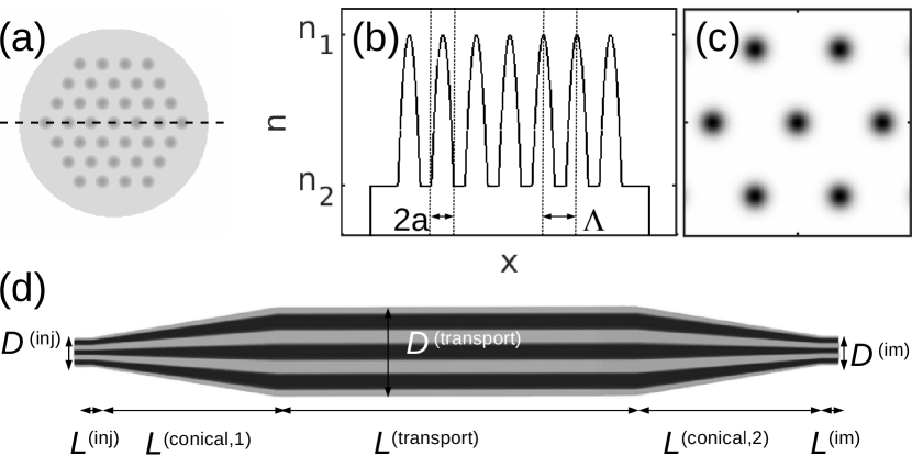
Figure 1: Sketch of tapered MCF (shown with reduced core count, for compactness). (a) Structure of MCF with triangular core layout. (b) Refractive index profile along the dashed line in (a). $a$, core diameter. $\Lambda$, pitch. $n_{1}$ Core refractive index. $n_{2}$ Cladding refractive index. (c) Example image of intensity emerging from the distal end facet of the tapered MCF showing the fundamental mode of seven cores. (d) Taper profile of the tapered MCF. From the left, injection segment of constant diameter $D^{(\mathrm{inj})}$ and length $L^{(\mathrm{inj})}$; first conical segment of length $L^{(\mathrm{conical,1})}$; transport segment of diameter $D^{(\mathrm{transport})}$ and length $L^{(\mathrm{transport})}$; second conical segment of length $L^{(\mathrm{conical,2})}$ ; imaging segment of diameter $D^{(\mathrm{im})}$ and length $L^{(\mathrm{im})}$.

3 Results

3.1 Coupled-mode theory model

To assist in the identification of the optimal design parameters, we developed a code, based on coupled-mode theory (CMT) and perturbation theory, which we refer to as the ”CMT model”, and which is available as part of Dataset 1, Ref. 15. The CMT model considers the tapered MCF as a concatenation of uniform segments and requires the structural parameters of these segments. It returns the effective indices of the guided modes as well as its transmission matrix (TM) ${\mathbf{H}}$ which it calculates as the product of segment TMs: $\mathbf{H}$ = $\prod_{i}{\mathbf{H}}_{i}$ (Suppl. Doc. Sec. A). The TM $\mathbf{H}$ is expressed in the basis of the fundamental modes of the $N$ cores and is of dimension $N\times N$ (higher-order modes—if present—are simply left out). $\mathbf{H}$ alone allows to predict the cross-talk (XT, a measure of the energy exchanged among cores) in terms of the $N\times N$ ”cross-talk matrix” (sometimes called the ”power transfer matrix”) $\mathbf{X}$ here defined as

$$\mathbf{X}=\langle|\mathbf{H}|^{2}\rangle_{\lambda}$$ (1)

where the average over $\lambda$ is the average over a sufficiently large number of calculated TMs for different wavelengths (cf the experimental measurement with a filtered—about 10 nm spectral width—incoherent source); and the scalar ”average total cross-talk” $X_{\mathrm{ave}}$

$$X_{\mathrm{ave}}=\frac{1}{N}\sum_{i}(\sum_{j\neq i}X_{ij}).$$ (2)

In parallel with the CMT model, we developed a model based on the finite-element beam propagation method (FE-BPM) [16, 17] (Suppl. Doc. Sec. B) which we refer to as ”the FE-BPM model”. Unlike CMT, FE-BPM makes no prior assumptions on the modes of the MCF and so is generally the more accurate of the two. It is however much slower. Here, we have used the FE-BPM model as a ”gold standard” against which we have compared the results of the CMT model. In Fig. 2(a) and 2(b) we present XT matrices for a $N$ = 475 core MCF as predicted by the CMT model and the FE-BPM model respectively which look qualitatively and quantitatively similar. The XT preferentially occurs between neighbor cores. This is not easy to see from the Figure because the core numbering convention influences the appearance of the Figure. Typically, in the modelled case there is significant XT ($X_{ij}>-30$ dB) between cores up to 5$\Lambda$ apart. From this comparison we establish the accuracy of the CMT model up to average total cross-talk of at least $X_{\mathrm{ave}}$ = -2 dB and down to effective indices 0.8e-3 above the cladding index.

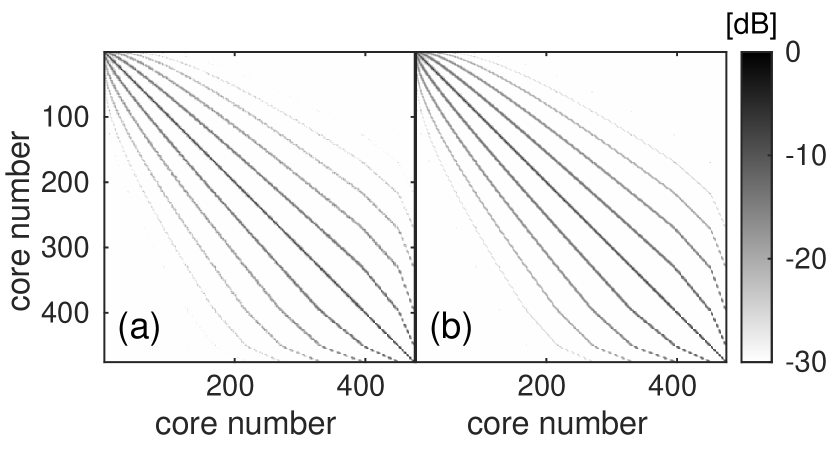
Figure 2: XT matrix $\mathbf{X}$ of a uniform MCF segment computed by (a) CMT model; and (b) FE-BPM model at 800 nm. Core numbering convention, the center core is number 1, the six cores in the first hexagonal ring are 2–7, etc. Simulation parameters: $L$ = 5 mm; $N$ = 475; $\Lambda$ = 7.5 $\upmu$m; $a$ = 1.4 $\upmu$m.

The CMT model also returns the field of the fundamental core mode vs the radial coordinate; it can be interpolated on the cartesian ”distal pixel basis” $\{x^{(\mathrm{dist})}_{j},y^{(\mathrm{dist})}_{j}\},1\leq j\leq N_{\mathrm{pix}}$; centering $N$ copies on the core positions $(x^{(\mathrm{core})}_{j},y^{(\mathrm{core})}_{j}),1\leq j\leq N$ ; each of these can be numerically propagated (assuming free-space propagation) to the far-field by a two-dimensional discrete Fourier transform, the resulting fields are expressed in the (angular) ”far-field pixel basis” $\{f^{(\mathrm{FF})}_{x,j},f^{(\mathrm{FF})}_{y,j}\},1\leq j\leq N_{\mathrm{pix}}$; and finally re-arranged to a mode-to-far-field pixel basis change matrix $\mathbf{U}$ of dimensions $N\times N_{\mathrm{pix}}$. $\mathbf{U}$ together with $\mathbf{H}$ permit to calculate ${\mathbf{e}}^{(\mathrm{FF,pix})}$ of dimensions $N_{\mathrm{pix}}\times 1$ the field in the far-field of the MCF distal end face

$${\mathbf{e}}^{(\mathrm{FF,pix})}={\mathbf{U}}^{\dagger}\mathbf{H}{\mathbf{e}}^{(\mathrm{prox,mode})}$$ (3)

where ${\mathbf{e}}^{(\mathrm{prox,mode})}$ is $N\times 1$ and contains elements representing the complex modal field amplitudes injected into the proximal end of the MCF. It is from the vector ${\mathbf{e}}^{(\mathrm{FF,pix})}$ that the properties of Strehl ratio (a measure of the intensity in the distal focus relative to the total intensity) and the memory effect (a measure of input-output angular correlations allowing distal point-scanning by proximal angular scanning) [18] can be inferred. ${\mathbf{e}}^{(\mathrm{FF,pix})}$ can also be numerically propagated to any intermediate plane with an angular spectrum propagator if required. The elements of the $N\times 1$ vector ${\mathbf{e}}^{(\mathrm{prox},\mathrm{mode},j_{0})}$ are the optimal input modal amplitudes to obtain an optimal focus on far-field pixel $j_{0}$ and is found as the conjugate transpose of the $j_{0}$’th row of $\mathbf{U}^{\dagger}\mathbf{H}$. ${\mathbf{e}}^{(\mathrm{FF,pix,j_{0}})}$ is the resulting complex field optimally focused on far-field pixel $j_{0}$ which is found by applying Eq. (3). The Strehl ratio $S$ can then be defined as the ratio of the energy in the focus on far-field pixel $j_{0}$ to the total energy in the field, for example by plotting the norm-square of ${\mathbf{e}}^{(\mathrm{FF,pix,j_{0}})}$ versus $\{f^{(\mathrm{FF})}_{x,j},f^{(\mathrm{FF})}_{y,j}\}$ and integrating over the focus area and then over the whole field. The so-called ”memory effect” is the effect by which the direction (phase ramp) of the output field changes by the same amount as the direction (phase ramp) of an input field [18]. In presence of the memory effect, it is therefore possible to displace a distal focus by simply adding a phase ramp to the proximal field. ${\mathbf{p}}(f^{(0)}_{x},f^{(0)}_{y})$ is $N\times 1$ and its elements are the [complex exponentials of] additional proximal modal phases required to move the focus in the far-field by $(f^{(0)}_{x},f^{(0)}_{y})$ using the memory effect:

$$\mathbf{p}(f^{(0)}_{x},f^{(0)}_{y}):p_{k}(f^{(0)}_{x},f^{(0)}_{y})=\mathrm{exp}(i2\pi f^{(0)}_{x}x_{k}^{(\mathrm{core})}+i2\pi f^{(0)}_{y}y_{k}^{(\mathrm{core})})$$ (4)

The memory effect can then be quantified as a two-dimensional curve $M(f^{(0)}_{x},f^{(0)}_{y})$ which is a ratio, the denominator containing the intensity of the field ”optimally focused on far-field pixel $j_{1}$” ${\mathbf{e}}^{(\mathrm{FF,pix,j_{1}})}$; and the numerator containing the intensity of the field ”initially optimally focused on far-field pixel $j_{0}$ then shifted to far-field pixel $j_{1}$ using the memory effect”:

$${\mathbf{e}}^{(\mathrm{FF,pix},j_{0}\rightarrow j_{1})}={\mathbf{U}}^{\dagger}\mathbf{H}[{\mathbf{h}}^{(j_{0})}\circ{\mathbf{p}}(f^{(0)}_{x},f^{(0)}_{y})]$$ (5)

where ”$\circ$” signifies Hadamard product (element-by-element multiplication). $M$ is constant = 1 for ”full” memory effect, and = 0 everywhere except the origin for ”no” memory effect.

As outlined above, the quantities $X_{\mathrm{ave}}$, $S$, and $M$ represent properties of tapered MCF that can be predicted by the CMT model from the tapered MCFs structural properties. Inversely, the CMT model can be used to identify the tapered MCF designs that result in a chosen set of properties.

3.2 Target properties and identification of target designs

The objective is to identify the design parameters cf Fig. 1(d) of a tapered MCF with triangular core layout with suitable properties for two-photon lensless imaging with a pulsed 920 nm excitation laser—the method would also work for any other core layout one has the capacity to fabricate.

As a first step, we want to minimize inter-core group delay dispersion in the transport segment cf Fig. 1(d) (center) which is debilitating for the short-pulsed excitation that we aim for. This dispersion arises from local variations among cores. We identify the rule-of-thumb that inter-core group delay dispersion decreases with increasing $V$-parameter. This holds for all the hypothesized physical origins that we considered ([19, 20, 21] and Suppl. Doc. Sec. D). We therefore choose to constrain the $V$-parameter to around 5.06, the second cutoff of a parabolic-index core, making the core bi-mode. To avoid exciting the higher-order mode in the transport segment, we decide to add an ”injection” segment separated cf Fig. 1(d) (left) from the transport segment by a conical taper whose dimensions are scaled by the factor $t^{(\mathrm{inj})}$ = 0.6 resulting in $V$ = 3.0 which is comfortably below the single-mode cutoff ($V_{\mathrm{cutoff}}$ = 3.518). Next we want to fix the refractive index step, core size, and pitch in the transport segment with the aim of keeping $X_{\mathrm{ave}}$ very low, say, below -25 dB in one metre of MCF. To this end, the refractive index step should generally be chosen as high as practically possible, $\Delta n$ = 30$\cdot$10^-3; to conserve $V$ = 5 the radius must then be chosen $a$ = 2.5 $\upmu$m. The only parameter left is the pitch $\Lambda$. We use the CMT model to predict that the chosen criterion on $XT_{\mathrm{ave}}$ is respected for $\Lambda~{}>~{}14~{}\upmu$m (predicted $X_{\mathrm{ave}}$ = -62 dB per metre in the uniform segment, -26 dB in the injection segment with $t^{(\mathrm{inj})}$ = 0.6). At this point the number of cores $N$ can be fixed. It may be chosen arbitrarily, generally ”the more the better” as the number of resolvable image pixels is proportional to $N$. Other than that $N$ only impacts on the outer diameter of the transport section, so it can be chosen so as to respect a chosen condition on the outer diameter. Here, we choose $N$ = 349, resulting in an outer diameter $D^{(\mathrm{transport})}$ = 330 $\upmu$m. Finally, and most importantly, we now want to choose the dimensions of the imaging segment cf Fig. 1(d) (right). All of its structural parameters are scaled by the factor $t^{(\mathrm{im})}$ relative to those of the transport segment. We are particularly interested in two values, a first one which maximizes the Strehl ratio under the condition that the ”full” memory effect is conserved; and a second one which maximizes the Strehl ratio without any conditions on the memory effect. But in this case a new condition must be respected, that core guidance is maintained, i.e. the effective indices of all modes must remain comfortably above the cladding index so as not to be too close to the single-mode cutoff. In Fig. 3(d) we present the curves of memory effect for different $t^{(\mathrm{im})}$; in Fig. 3(e) the Strehl ratio; in Fig. 3(f) the effective indices; and in Fig. 3(g) the average XT as functions of $t^{(\mathrm{im})}$ as predicted by the CMT model (the rest of the parameters are as in Tab. 1). Based on the following discussion we identify $t^{(\mathrm{im})}$ = 0.6 (maximum Strehl ratio while retaining full memory effect) and 0.4 (maximum Strehl ratio while retaining core guidance) respectively.

Fig. 3(a)-3(c) present the predicted point-spread functions (PSF) at distance $Z$ = $Z_{0}\cdot t^{(\mathrm{im})}$ from the distal end of the MCFs with $Z_{0}$ = 500 $\upmu$m and $t^{(\mathrm{im})}$ = 1, 0.6, and 0.4 (per se they are far-field images scaled by $x$ = $f_{x}Z\lambda$, $y$ = $f_{y}Z\lambda$). It comprises a central spot surrounded by a dimmer periodic replicas for untapered MCF ($t^{(\mathrm{im})}$ = 1). However, it becomes more singly-peaked, very beneficial for image quality, as the taper ratio decreases while the focal spot size which is represented by the full-width at half-maximum (FWHM) of the PSF is fairly constant equal to 2.4 $\upmu$m. From Fig. 3(f) which shows the predictions of effective indices it can be seen that at $t^{(\mathrm{im})}$ = 0.3 some of the indices drop below the cladding index (lower dashed line) making leaking to cladding modes inevitable. This is the reason the lowest value of $t^{(\mathrm{im})}$ retained as design parameter was 0.4 for which effective indices remain 2$\cdot$10^-3 above the cladding index. Another important consequence of tapering, of primordial importance for two-photon imaging, is the dramatic increase in the Strehl ratio with decreasing taper ratio as shown in Fig. 3(e).

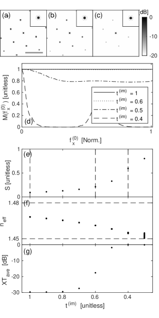
Figure 3: Properties of tapered MCF predicted by CMT model. (a)-(c) PSF for $t^{(\mathrm{im})}$ = 1.0, 0.6, and 0.4 in a plane $Z$ = $Z_{0}\cdot t^{(\mathrm{im})}$. Each image is normalized to its maximum intensity. Scale bar, 50 $\upmu$m. Insets, 5$\times$ zoom on the central spot. (d) Memory effect curves. Horizontal axis normalized to half the distance between replica spots. (e) Strehl ratio. (f) Effective indices of supermodes. (g) Average XT. Unmentioned parameters are as in Tab. 1.

3.3 Fabrication and characterization of target designs

We fabricated a MCF to the specification requirement of the transport segment identified in Sec. 3.2 ($\Delta n$ = 30$\cdot 10^{-3}$; $\Lambda$ = 14 $\upmu$m; $a$ = 2.5 $\upmu$m; $N$ = 349) by the methods we used previously (Ref. 13 and Suppl. Doc. Sec. C).

Then we post-processed the uniform MCF to obtain the tapered MCF represented by Fig. 1(d) by tapering a short length at the terminals of the MCF using a CO₂ laser-based glass processing and splicing system (LZM-100 FUJIKURA) (Suppl. Doc. Sec. E). The MCF is locally heated up with the CO₂ laser and simultaneously pulled lengthwise by stepper motors so as to obtain a fiber whose diameter varies longitudinally. This system provides extremely stable operation and allows control over a wide range of parameters to achieve the tapered MCFs precisely with the chosen design parameters Tab. 1.

Identifier	0	1	2
$D^{(\mathrm{inj})}$ [$\upmu$m]	196	194	196
$t^{(\mathrm{inj})}$	0.6	0.6	0.6
$L^{(\mathrm{inj})}$ [m]	0.005	0.005	0.005
$L^{(\mathrm{conical,1})}$ [m]	0.025	0.025	0.025
$D^{(\mathrm{transport})}$ [$\upmu$m]	330	330	330
$L^{(\mathrm{transport})}$ [m]	0.23	0.21	0.24
$L^{(\mathrm{conical,2})}$ [m]	0	0.05	0.05
$D^{(\mathrm{im})}$ [$\upmu$m]	330	199	135
$t^{(\mathrm{im})}$	1	0.6	0.4
$L^{(\mathrm{im})}$ [m]	0	0.005	0.005

Table 1: The physical dimensions of the fabricated tapered MCF samples.

We characterized the optical properties of the fabricated tapered MCF using a filtered super-continuum laser source (Suppl. Sec. F). We injected the focused laser beam into MCF cores in the injection segment successively, and imaged the emerging beam out of imaging segment on a camera. Consequently, we could measure the mode field diameter (MFD) of the visualized mode profile and confirm—for each $t^{(\mathrm{im})}$—the agreement with the predictions of the CMT model. Additionally we were able to measure the XT between excited core and other cores and thus build up $\mathbf{X}$ in the core basis which is presented in Fig. 4(f) and which agrees reasonably with the predicted values in Fig. 3(g). To confirm that the tapered MCFs were effectively single-mode with the choice of injection segment parameters, we tested a long MCF ($L^{(\mathrm{transport})}>~{}1$ m) with $t^{(\mathrm{inj})}$ = 0.6 and $t^{(\mathrm{im})}$ = 1. On the camera we visualized the intensity profile exiting one core and verified that it did not change while applying a perturbation on the fiber. This verifies that only the fundamental mode propagates through the transport segment despite it being bi-modal, thus the injection segment allows the selective excitation of only the fundamental mode of each core.

3.4 Two-photon imaging lensless endoscope

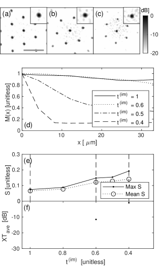
Figure 4: Experimentally observed properties of the tapered MCFs with parameters given in Tab. 1; the parameters of the two tapered MCFs with $t^{(\mathrm{im})}$ = 0.8 and 0.5 not appearing in the Table are very similar. (a)–(c) PSF for $t^{(\mathrm{im})}$ = 1, 0.6, and 0.4 in a plane $Z$ = $Z_{0}\cdot t^{(\mathrm{im})}$ = 500, 300, and 200 $\upmu$m. Insets, 5$\times$ zoom on the central spot. Each image is normalized to its maximum intensity. Scale bar, 50 $\upmu$m. (d) Memory effect curves. (e) Strehl ratio. (f) Average cross-talk.

As a first step towards implementing the tapered MCFs in a lensless endoscope system we measured the imaging properties of the fabricated tapered MCFs. The measurements were done using a pulsed fs-laser shaped by a spatial-light modulator (SLM) for injection while measuring the resulting intensity distributions in a plane a distance $Z$ from the distal end face. The SLM was programmed to generate the focus (Suppl. Doc. Sec. G). The experimentally measured properties are presented in Fig. 4 and organized in the same way as the Figure of predicted properties, Fig. 3. Figures 4(a)–4(c) show the PSFs with $t^{(\mathrm{im})}$ = 1, 0.6, and 0.4 and $Z$ = $Z_{0}\cdot t^{(\mathrm{im})}$ = 500 $\upmu$m, 300 $\upmu$m, and 200 $\upmu$m. The measured FWHMs of the PSFs are 4.2, 4.0, and 3.6 $\upmu$m, slightly larger than predicted. The rest of the observed trends are in line with the predictions, that is, increasing intensity in the central focus and decreasing intensity in the satellite peaks as $t^{(\mathrm{im})}$ is decreased. This trend is quantified in the measured Strehl ratio, presented in Fig. 4(e), from a value of 7 % at $t^{(\mathrm{im})}$ = 1, it increases to 15 % at $t^{(\mathrm{im})}$ = 0.6 and reaches 19 % at the smallest value of $t^{(\mathrm{im})}$ = 0.4. In terms of absolute power in focus these values correspond to 20, 43, and 54 mW. The experimentally measured memory effect curves are presented in Fig. 4(d). The taper ratios $t^{(\mathrm{im})}$ = 1, 0.6, and 0.4 were identified as key values in Sec. 3.2, the first assuring maximum memory effect, the second assuring the highest Strehl ratio while preserving significant memory effect, and the final assuring highest Strehl ratio regardless of memory effect. The Fig. 4(d) confirms these predictions, as the curves $t^{(\mathrm{im})}$ = 1 and 0.6 are coincident and almost constant equal to 1 testifying to an almost identical memory effect. On the other hand, the curve $t^{(\mathrm{im})}$ = 0.4 strongly peaked around $x$ = 0 testifies to an almost complete absence of memory effect but the highest Strehl ratio as seen from Fig. 4(e).

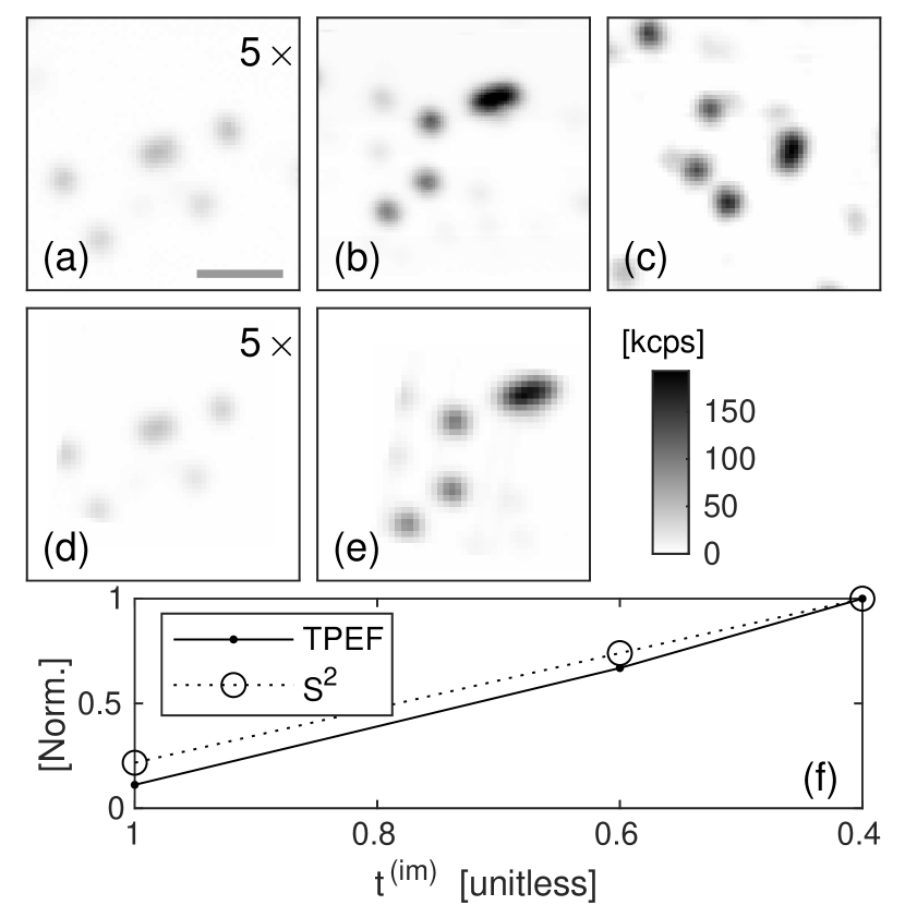
Figure 5: Two-photon excited fluorescence images of fluorescent beads with the lensless endoscope. (a)-(c) Point-scanning with an optimal focus on each pixel (TM scan) and taper ratios (a) $t^{(\mathrm{im})}$ = 1 and $Z$ = 500 $\upmu$m; (b) $t^{(\mathrm{im})}$ = 0.6 and $Z$ = 300 $\upmu$m; and (c) $t^{(\mathrm{im})}$ = 0.4 and $Z$ = 200 $\upmu$m. (d)-(e) Point-scanning with memory effect starting from an optimal focus on the central pixel (ME scan) and taper ratios (d) $t^{(\mathrm{im})}$ = 1; and (e) $t^{(\mathrm{im})}$ = 0.6. Spatial scales are identical for all the images. Intensities in (a) and (d) have been multiplied by 5 for visualization. Scale bar, 10 $\mu$m. (f) Evolution of two-photon signal with taper ratio. (dots) Observed two-photon signals; and (circles) the square of the observed Strehl ratios.

The formation of a two-photon fluorescence image in a lensless endoscopy system requires a single-point detector to acquire the two-photon fluorescence generated by the sample; and a raster scanning scheme where the focus is scanned across two dimensions. This can be realized in two different ways, either (i - ”TM scan”) the phases of the elements of a pre-measured TM can be converted to SLM masks which scan the focus across the sample when displayed sequentially on the SLM; or (ii - ”memory effect (ME) scan”) a focus initially on a center pixel can be displaced by the memory effect and scanned across the sample, this is done through the addition of a sequence of suitable phase ramps in a conjugate plane of the proximal MCF end face (Suppl. Sec. G). When possible, the ME scan method has the dual advantage of not requiring knowledge of a full TM; and the possibility to use fast galvo mirrors to generate the phase ramps (virtually unbound image acquisition time [13]). With the different tapered MCFs in our lensless endoscope system, we performed two-photon imaging with both the TM scan method and the ME scan method. For simplicity and pragmatism, here, we used the SLM for both (so we are unable to demonstrate the speed advantage). For these proof-of-principle demonstrations, we used yellow-green fluorescent beads as a sample whose emission spectrum is similar to that of yellow fluorescent proteins commonly expressed e.g. in mice neurons during in-vivo exploration of neuronal activity. The acquired two-photon images are presented in Fig. 5. The upper row Figs. 5(a)-5(c) show two-photon images acquired using the TM scan method with $t^{(\mathrm{im})}$ = 1, 0.6, and 0.4. The second row Figs. 5(d), 5(e) show two-photon images acquired using the ME scan method with $t^{(\mathrm{im})}$ = 1 and 0.6. The comparison to Figs. 5(a), 5(b) provides visual evidence that the memory effect is indeed retained at these values, as predicted. No image with the ME scan is shown for $t^{(\mathrm{im})}$ = 0.4 because the ME is absent. All images are on the same intensity scale which allows to appreciate the increase in two-photon signal with decreasing $t^{(\mathrm{im})}$. It can be seen that the signal from single, isolated beads increases appreciably from Fig. 5(a) over 5(b) to 5(c). This two-photon signal increase is quantified in Fig. 5(f). The points represent a mean over two-photon signal measured on several single, isolated beads. The relative increases are a factor 6.0 and a factor 8.9 for $t^{(\mathrm{im})}$ = 0.6 and 0.4. The two-photon signal increase is expected to be proportional to the square of the Strehl ratio, represented by circles. And indeed the two curves are coincident to a high degree.

4 Discussion

Initially, we remark that for the experimental two-photon imaging, only 169 out of the $N$ = 349 cores of the tapered MCFs were employed simultaneously. An experimental constraint limiting the number of cores that can be used simultaneously is the number of pixels on the SLM. A 800$\times$600 pixel SLM can be divided into 169 40$\times$40 pixel segments which must control not only the phase but also the focusing of light injected into a core (Suppl. Sec. G), and the latter is compromised as the number of pixels per segment decreases. So, while not a hard limit, 169 cores was the compromise we chose. Workarounds are to use one of the newer SLM generations with higher pixel count; or using the SLM in conjunction with a passive elements like a micro-lens array to take care of the focusing. The modelling was limited to the same number of cores ($N$ = 169) in order to have directly comparable results.

Next, we remark that the CMT model has not correctly predicted the experimentally measured Strehl ratios [Fig. 3(e) compared to Fig. 4(e)]. For $t^{(\mathrm{im})}$ = 0.6 the prediction is $S$ = 21 % versus the observed $S$ = 15 %. This discrepancy can be accounted for by two factors not included in the model. (i) Polarization is not accounted for in the CMT model, but the fabricated tapered MCF has circular ie non-polarization-maintaining cores. In the experiment a polarizer selects one of the polarization components, each core thus contributes a random amplitude to the image on the camera. The effect can be modelled by multiplying each element of ${\mathbf{e}}^{(\mathrm{prox},\mathrm{mode},j_{0})}$ by a random number between zero and one before applying Eq. (3), and the consequence is a drop of $S$ down to 18 %. (ii) The model calculates the Strehl ratio in the far-field whereas the experiments were done in intermediate planes $Z$ = 500, 300, and 200 $\upmu$m. The predicted Strehl ratio should therefore be taken as upper bounds. If we numerically propagate the predicted far-field to the intermediate plane, this effect alone leads to a drop of $S$ down to 16.5 %. Both effects together result in a drop of $S$ to 12 %. These effects thus seem to fully explain the discrepancy. For $t^{(\mathrm{im})}$ = 0.4 the discrepancy is more flagrant, the prediction is $S$ = 59 % versus the observed $S$ = 19 %. Here; effects (i) and (ii) combined would only result in a drop of $S$ down to 42 %. It is possible that at this small value of $t^{(\mathrm{im})}$ the effect of leakage from the cores into the cladding becomes important. This would signify that the CMT model is at the limit of or even beyond its regime of validity for $t^{(\mathrm{im})}$ = 0.4. Beyond this point one would have to resort to FE-BPM modelling to assure accurate results (using, for example, the open source FE-BPM tool in Ref. 22).

Inter-core group delay dispersion (GDD) [21] is also not accounted for in the CMT model. Non-zero inter-core group delay dispersion has the consequence of reducing the coherence between the fields emerging from different cores (since we are using ultra-short pulses) and hence the Strehl ratio. We have sampled inter-core GDD in some pairs of cores which indicate that the distribution of inter-core GDD is narrower than the duration (150 fs) of the ultra-short laser pulse. This is not expected to be a main source of the discrepancy in Strehl ratios and the above discussion corroborates this.

We must remark that the lensless endoscope system used to generate Figs. 4 and 5 employed a detector located at the distal end, after both MCF and sample, rather than at the proximal end as it would in a ”true” endoscopic configuration, detecting fluorescence collected in the backward direction through the MCF. In a previous paper we did demonstrate how a double-clad MCF allows for efficient fluorescence collection and thus to work with a proximal detector only [10], where the double-cladding was a ring of air holes around the $N$ cores. However we were unable to use the same kind of double cladding in the present work because the post-processing on the glass processing and splicing system would have collapsed the air holes. In the near term our aim is to realize versions of the tapered MCF presented above with double cladding. We envisage that coating the tapered MCFs with low-index polymer as a final step will achieve this effect.

One of the biggest challenges facing lensless endoscopes—be they multi-mode fiber-based or MCF-based—is the resilience to bending or lack thereof. Conformational changes of a multi-mode fiber or MCF generally alters its TM significantly, meaning that re-performing the initial calibration steps is mandatory after each conformational change, which becomes unfeasible even for slow conformational changes. The tapered MCFs presented above are also subject to this problem—even though we previously showed that bending a MCF results in a predictable phase ramp which only shifts the focus without degrading it [23]. In a more recent paper [14] we reported the fabrication of a helically-twisted MCF and demonstrated that it is invariant to conformational changes in a fairly wide range of operational conditions when used in a lensless endoscope system. The fabrication method of the tapered MCFs outlined in the present paper takes as its starting point a standard (ie not helically twisted) MCF. But there would be no conceptual difficulties starting from a helically-twisted MCF instead. As such the pursuit of conformationally-invariant tapered MCFs also represents a near-term aim.

5 Conclusion

We have presented a novel tapered MCF for optimal two-photon lensless endoscopy by point-scanning imaging. Our key result is that optimized tapered MCF can increase two-photon yield by a factor 6.0 while still keeping the ability to point-scan by the memory effect, and up to a factor 8.9 while sacrificing the memory effect. These results are decoupled from the transport segment of the tapered MCF with low XT which can be metres in length without altering the results. We have outlined the entire procedure of conception, design, fabrication, and application in a lensless endoscopy system of this novel fiber-optic component. The procedure, namely the step involving the CMT model, is generic and applicable to other ranges of properties, other MCF core layouts e.g. a Fermat golden spiral layout [24], wavelength ranges, etc. We conclude that tailoring of the taper profile is a degree of freedom that can be efficiently exploited for ameliorating MCF based lensless endoscopes and we have shown here that it contributes to solving the major power delivery issue that MCF based lensless endoscopes [25]. More generally a tapered multi-core fiber is a valuable add-on into the lensless endoscope toolbox to design, optimize and fabricate ultra-miniaturized endoscope tailored to a broad range of applications.

6 Backmatter

Funding
Agence Nationale de la Recherche (ANR-11-IDEX-0001-02, ANR-20-CE19-0028, ANR-21-ESRS-0002 IDEC, ANR-21-ESRE-0003 CIRCUITPHOTONICS); INSERM (18CP128-00, PC201508); Centre National de la Recherche Scientifique, Aix-Marseille Université (A-M-AAP-ID-17-13-170228-15.22-RIGNEAULT); National Institute of Health (NIH R21 EY029406-01).

Acknowledgments
Parts of this work were developed at IRCICA (USR CNRS 3380, https://ircica.univ-lille.fr/) using FiberTech Lille facilities (https://fibertech.univ-lille.fr/en/). This work was supported by the French Ministry of Higher Education and Research, the ”Hauts de France” Regional Council, the European Regional Development fund (ERDF) through the CPER ”Photonics for Society”.

Disclosures
The authors declare no conflicts of interest.

Supplemental document
See Supplement 1 for supporting content.

References

- [1] D. Psaltis and C. Moser, “Imaging with multimode fibers,” Opt. Photon. News 27, 24–31 (2016).
- [2] E. R. Andresen, S. Sivankutty, V. Tsvirkun, G. Bouwmans, and H. Rigneault, “Ultrathin endoscopes based on multicore fibers and adaptive optics: a status review and perspectives,” J. Biomed. Opt. 21, 121506 (2016).
- [3] S. Turtaev, I. T. Leite, T. Altwegg-Boussac, J. M. P. Pakan, N. L. Rochefort, and T. Čižmar, “High-fidelity multimode fibre-based endoscope for deep brain in vivo imaging,” Light Sci. Appl. 7, 92 (2018).
- [4] S. A. Vasquez-Lopez, R. Turcotte, V. Koren, M. Plöschner, Z. Padamsey, M. J. Booth, T. Čižmar, and N. J. Emptage, “Subcellular spatial resolution achieved for deep-brain imaging in vivo using a minimally invasive multimode fiber,” Light Sci. Appl. 7, 110 (2018).
- [5] S. Ohayon, A. Caravaca-Aguirre, R. Piestun, and J. J. DiCarlo, “Minimally invasive multimode optical fiber microendoscope for deep brain fluorescence imaging,” Biomed. Opt. Express 9, 1492–1509 (2018).
- [6] A. J. Thompson, C. Paterson, M. A. A. Neil, C. Dunsby, and P. M. W. French, “Adaptive phase compensation for ultracompact laser scanning endomicroscopy,” Opt. Lett. 36, 1707–1709 (2011).
- [7] T. Čižmár and K. Dholakia, “Shaping the light transmission through a multimode optical fibre: complex transformation analysis and applications in biophotonics,” Opt. Express 19, 18871–18884 (2011).
- [8] Y. Choi, C. Yoon, M. Kim, T. D. Yang, C. Fang-Yen, R. R. Dasari, K. J. Lee, and W. Choi, “Scanner-free and wide-field endoscopic imaging by using a single multimode optical fiber,” Phys. Rev. Lett. 109, 203901 (2012).
- [9] I. N. Papadopoulos, S. Farahi, C. Moser, and D. Psaltis, “Focusing and scanning light through a multimode optical fiber using digital phase conjugation,” Opt. Express 20, 10583–10590 (2012).
- [10] E. R. Andresen, G. Bouwmans, S. Monneret, and H. Rigneault, “Two-photon lensless endoscope,” Opt. Express 21, 20713–20721 (2013).
- [11] Y. Kim, S. C. Warren, J. M. Stone, J. C. Knight, M. A. A. Neil, C. Paterson, C. W. Dunsby, and P. M. W. French, “Adaptive multiphoton endomicroscope incorporating a polarization-maintaining multicore optical fibre,” IEEE J. Sel. Top. Quantum. Electron. 22, 171–178 (2016).
- [12] D. B. Conkey, N. Stasio, E. E. Morales-Delgado, M. Romito, C. Moser, and D. Psaltis, “Lensless two-photon imaging through a multicore fiber with coherence-gated digital phase conjugation,” J. Biomed. Opt. 21, 045002 (2016).
- [13] E. R. Andresen, G. Bouwmans, S. Monneret, and H. Rigneault, “Toward endoscopes with no distal optics: video-rate scanning microscopy through a fiber bundle,” Opt. Lett. 38, 609–611 (2013).
- [14] V. Tsvirkun, S. Sivankutty, K. Baudelle, R. Habert, G. Bouwmans, O. Vanvincq, E. R. Andresen, and H. Rigneault, “Flexible lensless endoscope with a conformationally invariant multi-core fiber,” Optica 6, 1185–1189 (2019).
- [15] “Dataset 1,” Https://XXX.
- [16] B. M. A. Rahman and A. Agrawal, Finite element modeling methods for photonics (Artech house, 2013).
- [17] M. Koshiba and Y. Tsuji, “A wide-angle finite-element beam propagation method,” IEEE Photon. Technol. Lett. 8, 1208–1210 (1996).
- [18] I. Freund, M. Rosenbluh, and S. Feng, “Memory effects in propagation of optical waves through disordered media,” Phys. Rev. Lett. 61, 2328 (1988).
- [19] J. C. Roper, S. Yerolatsitis, T. A. Birks, B. J. Mangan, C. Dunsby, P. M. W. French, and J. C. Knight, “Minimizing group index variations in a multicore endoscope fiber,” IEEE Photon. Technol. Lett. 27, 2359–2362 (2015).
- [20] J. C. Roper, “Advances in multicore optical fibres for endoscopy,” Ph.D. thesis, University of Bath (2015).
- [21] E. R. Andresen, S. Sivankutty, G. Bouwmans, L. Gallais, S. Monneret, and H. Rigneault, “Measurement and compensation of residual group delay in a multi-core fiber for lensless endoscopy,” J. Opt. Soc. Am. B 32, 1221–1228 (2015).
- [22] M. Veettikazhy, A. K. Hansen, D. Marti, S. M. Jensen, A. L. Borre, E. R. Andresen, K. Dholakia, and P. E. Andersen, “Bpm-matlab: an open-source optical propagation simulation tool in matlab,” Opt. Express 29, 11819–11832 (2021).
- [23] V. Tsvirkun, S. Sivankutty, G. Bouwmans, O. Vanvincq, E. R. Andresen, and H. Rigneault, “Bending-induced inter-core group delays in multicore fibers,” Opt. Express 25, 31863–31875 (2017).
- [24] S. Sivankutty, V. Tsvirkun, O. Vanvincq, G. Bouwmans, E. R. Andresen, and H. Rigneault, “Nonlinear imaging through a fermat’s golden spiral multicore fiber,” Opt. Lett. 43, 3638–3641 (2018).
- [25] S. Sivankutty, A. Bertoncini, V. Tsvirkun, N. G. Kumar, G. Brévalle, G. Bouwmans, E. R. Andresen, C. Liberale, and H. Rigneault, “Miniature 120-beam coherent combiner with 3d-printed optics for multicore fiber-based endoscopy,” Opt. Lett. 46, 4968–4971 (2021).