Fast estimation of Kendall’s Tau and conditional Kendall’s Tau matrices under structural assumptions

Abstract

Kendall’s tau and conditional Kendall’s tau matrices are multivariate (conditional) dependence measures between the components of a random vector. For large dimensions, available estimators are computationally expensive and can be improved by averaging. Under structural assumptions on the underlying Kendall’s tau and conditional Kendall’s tau matrices, we introduce new estimators that have a significantly reduced computational cost while keeping a similar error level. In the unconditional setting we assume that, up to reordering, the underlying Kendall’s tau matrix is block-structured with constant values in each of the off-diagonal blocks. Consequences on the underlying correlation matrix are then discussed. The estimators take advantage of this block structure by averaging over (part of) the pairwise estimates in each of the off-diagonal blocks. Derived explicit variance expressions show their improved efficiency. In the conditional setting, the conditional Kendall’s tau matrix is assumed to have a constant block structure, independently of the conditioning variable. Conditional Kendall’s tau matrix estimators are constructed similarly as in the unconditional case by averaging over (part of) the pairwise conditional Kendall’s tau estimators. We establish their joint asymptotic normality, and show that the asymptotic variance is reduced compared to the naive estimators. Then, we perform a simulation study which displays the improved performance of both the unconditional and conditional estimators. Finally, the estimators are used for estimating the value at risk of a large stock portfolio; backtesting illustrates the obtained improvements compared to the previous estimators.

Keywords: Kendall’s tau matrix, block structure, kernel smoothing, conditional dependence measure.

MSC: Primary: 62H20; secondary: 62F30, 62G05.

1 Introduction

In dependence modeling, the main object of interest is the copula, which is a cumulative distribution function on $[0,1]^{p}$ with uniform margins, describing the links between elements of a $p$-dimensional random vector ${\mathbf{X}}$. However, the copula belongs to an infinite-dimensional space, and it is not easy to represent it as soon as $p$ is larger than $3$ or $4$. In such cases, finite-dimensional statistics becomes more useful to understand the dependence, the most well-known of them being Kendall’s tau matrix.

Kendall’s tau between two random variables $X_{i}$ and $X_{j}$, denoted by $\tau_{i,j}=\tau({\mathbb{P}}_{i,j})$, is defined as the probability of concordance between two independent replications from the distribution ${\mathbb{P}}_{i,j}$ of $(X_{i},X_{j})$ minus the probability of discordance. The equality $\tau({\mathbb{P}}_{i,j})=4\int C_{i,j}dC_{i,j}-1$ relates Kendall’s tau with the copula $C_{i,j}$ of $X_{i}$ and $X_{j}$; we refer to [26] for an extensive introduction to Kendall’s tau and copulas.

When a covariate ${\mathbf{Z}}\in{\mathbb{R}}^{d}$ is available, we can extend the definition of Kendall’s tau to this conditional setting. Conditional Kendall’s tau is then defined as $\tau_{i,j|{\mathbf{Z}}={\mathbf{z}}}:=\tau({\mathbb{P}}_{(i,j)|{\mathbf{Z}}={\mathbf{z}}})$, where ${\mathbb{P}}_{(i,j)|{\mathbf{Z}}={\mathbf{z}}}$ denotes the conditional law of $(X_{i},X_{j})$ given ${\mathbf{Z}}={\mathbf{z}}$, for some ${\mathbf{z}}\in{\mathbb{R}}^{d}$. In [7, 16, 36], smoothing-based estimators of conditional Kendall’s tau are studied. In [6], it is shown that the estimation of conditional Kendall’s tau can be written as a classification task; they proposed to use classification algorithms to estimate conditional Kendall’s tau. In [8], a regression-type model is used to estimate conditional Kendall’s tau in a parametric conditional framework. [2] uses conditional Kendall’s tau for hypothesis testing.

For a random vector ${\mathbf{X}}$, we define Kendall’s tau matrix by ${\mathbf{T}}:=[\tau_{i,j}]_{1\leq i,j\leq p}$, which contains all pairwise Kendall’s taus; respectively, in the conditional framework, a natural counterpart is conditional Kendall’s tau matrix, denoted by ${\mathbf{T}}_{|{\mathbf{Z}}={\mathbf{z}}}:=[\tau_{i,j|{\mathbf{Z}}={\mathbf{z}}}]_{1\leq i,j\leq p}$. Kendall’s tau matrix is especially useful for elliptical graphical models and their generalizations, see [3, 22]. In [24], a time-varying graphical model is studied using an estimate of conditional Kendall’s tau matrix. Kendall’s tau matrix plays an important role since it allows robust estimation of the dependence, and can be used to fit an appropriate copula [15]. In an elliptical distribution framework, it can also be used to estimate the Value at Risk of a portfolio, see [30, 33].

Estimation of the $p\times p$ Kendall’s tau matrix ${\mathbf{T}}$ becomes particularly challenging in the high-dimensional setting when $p$ is large. Simple use of the naive Kendall’s tau matrix estimator of all pairwise sample Kendall’s taus will result in noisy estimates with estimation errors piling up due to the estimates’ individual imprecision [11]. Over the past two decades, various regularization strategies have been proposed to reduce the aggregation of estimation errors. Ultimately, these methods all make certain assumptions on the underlying dependence structure, hereby reducing the number of free parameters to estimate.

In many instances, sparsity of the target matrix is assumed. For such settings, various (combinations of) thresholding and shrinkage methods have been proposed, see for example [4, 17, 32]. However, such assumptions are certainly not appropriate for the modeling of most financial data, e.g. market risk is reflected in all share prices and therefore their returns are certainly correlated. To this end, factor models are usually imposed, where the correlations depend on a number of common factors, which may or may not be latent, see [11, 12].

In [28], an alternative approach to estimating large Kendall’s tau matrices was introduced. They studied a model in which it is assumed that the set of variables could be partitioned into smaller clusters with exchangeable dependence. As such, after reordering of the variables by cluster, the corresponding Kendall’s tau matrix is block-structured with constant values within each block. Following naturally is an improved estimation by averaging all pairwise sample Kendall’s taus within each of the blocks. Additionally, they have proposed a robust algorithm identifying such structures (see also [29] for testing for the presence of such a structure).

In this article, we study a similar framework as in [28], where we relax the partial exchangeability assumption: we only assume that off-diagonal blocks of Kendall’s tau matrix are constant. One of the drawbacks of the estimator studied in [28] is its computational cost, which is close to the one of the naive Kendall’s tau matrix estimator: the number of pairwise sample Kendall’s taus that are to be computed scales quadratically with the dimension $p$.

Naturally, the idea of averaging among several Kendall’s taus can be applied to part of the blocks, which allows for faster computations. As such, we propose several estimators that average among part of the Kendall’s tau per off-diagonal block and study their efficiencies and computational costs. For every off-diagonal block, we will consider averaging over elements in the same row, averaging over elements on the diagonal and averaging over a number of randomly selected elements. We will be referring to these estimators as the row, diagonal and random estimators; the estimator that averages over all elements is referred to as the block estimator.

We then extend this model to the conditional setup: conditional Kendall’s taus are depending on ${\mathbf{z}}$ and are assumed to be clustered such that for all ${\mathbf{z}}\in{\mathbb{R}}^{d}$, the Kendall’s tau conditionally on ${\mathbf{Z}}={\mathbf{z}}$ between variables of different groups is only depending on group numbers and on the value of ${\mathbf{z}}$. In view of applications to finance, the conditional version of our structural assumption could, for example, be seen as assuming that the correlations between European stocks of two different groups are equal and react equally in changes of some other American stock or portfolio. Furthermore, in [1, 10, 23], it was shown that stock returns actually exhibit higher correlations during market declines than during market upturns, and moreover that the same applies to exchange rates in [27]. In such a model, it is also important to limit computation times and study improved estimators that can take advantage of the block structure of the Kendall’s tau matrix.

In this framework, we adopt nonparametric estimates of the conditional Kendall’s tau based on kernel smoothing. Based on these nonparametric estimates we introduce conditional versions of the averaging estimators and study their asymptotic behavior as the sample size $n$ tends to infinity. It is worth noting that conditional estimates of Kendall’s tau using kernel smoothing carry significantly more computational cost than their unconditional counterparts, especially when the covariate’s dimension $d$ is large. Therefore, faster computations of conditional Kendall’s tau matrices will be of particular use in the conditional, nonparametric setup.

The rest of this article is structured as follows. In Section 2, we present the unconditional framework, and detail a few consequences on the correlation matrix. Then we construct the different estimators in this framework, and derive variance expressions. Similarly, Section 3 is devoted to the improved estimation of the conditional Kendall’s tau matrix, where we propose averaged conditional estimators and we derive the estimators’ joint asymptotic normality. In Section 4 we perform a simulation study in order to support the theoretical findings. Finally, in Section 5, we examine a possible application to study the behavior of the estimators in real data conditions. The estimators are used for the robust inference of the covariance matrix to estimate the value at risk of a large stock portfolio. Most proofs are postponed to the Appendix.

Notations. We denote by ${\mathbf{1}}$ be the vector and the matrix with all entries equal to $1$, where the dimensions can be inferred from the context. For a matrix $M$ of size $p\times p$, and a set of indices $J\subset\{1,\dots,p\}^{2}$, we denote by $[M]_{J}$ the submatrix $(M_{j})_{j\in J}$.

2 Fast estimation of Kendall’s tau matrix

2.1 The Structural Assumption

Let $n\geq 0$ and assume that we observe $n$ i.i.d. replications $\mathbf{X}_{i}=(X_{i,1},\ldots,X_{i,p})$ of a random vector ${\mathbf{X}}=(X_{1},\dots,X_{p})\in{\mathbb{R}}^{p}$, for $i=1,\dots,n$. Moreover, assume that the Kendall’s tau matrix ${\mathbf{T}}:=[\tau_{i,j}]_{1\leq i,j\leq p}$ of ${\mathbf{X}}$ satisfies the following structural assumption.

Assumption A1 (Structural Assumption).

There exists $K>0$ and a partition $\mathcal{G}=\{\mathcal{G}_{1},\dots,\mathcal{G}_{K}\}$ of $\{1,\dots,p\}$, such that for all distinct $k_{1},k_{2}\in\{1,\dots,K\}$,

$$\left[{\mathbf{T}}\right]_{\mathcal{G}_{k_{1}}\times\mathcal{G}_{k_{2}}}=\tau_{k_{1},k_{2}}{\bf 1},$$

for some constants $\tau_{k_{1},k_{2}}\in[-1,1]$.

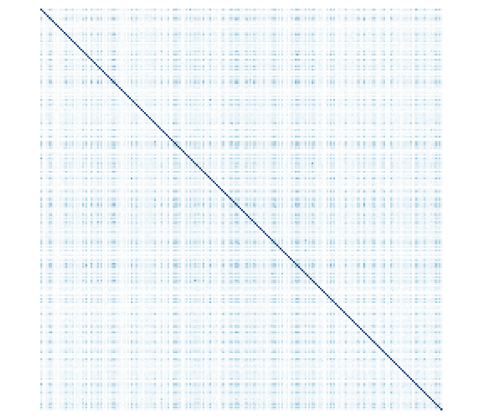
(a) unclustered

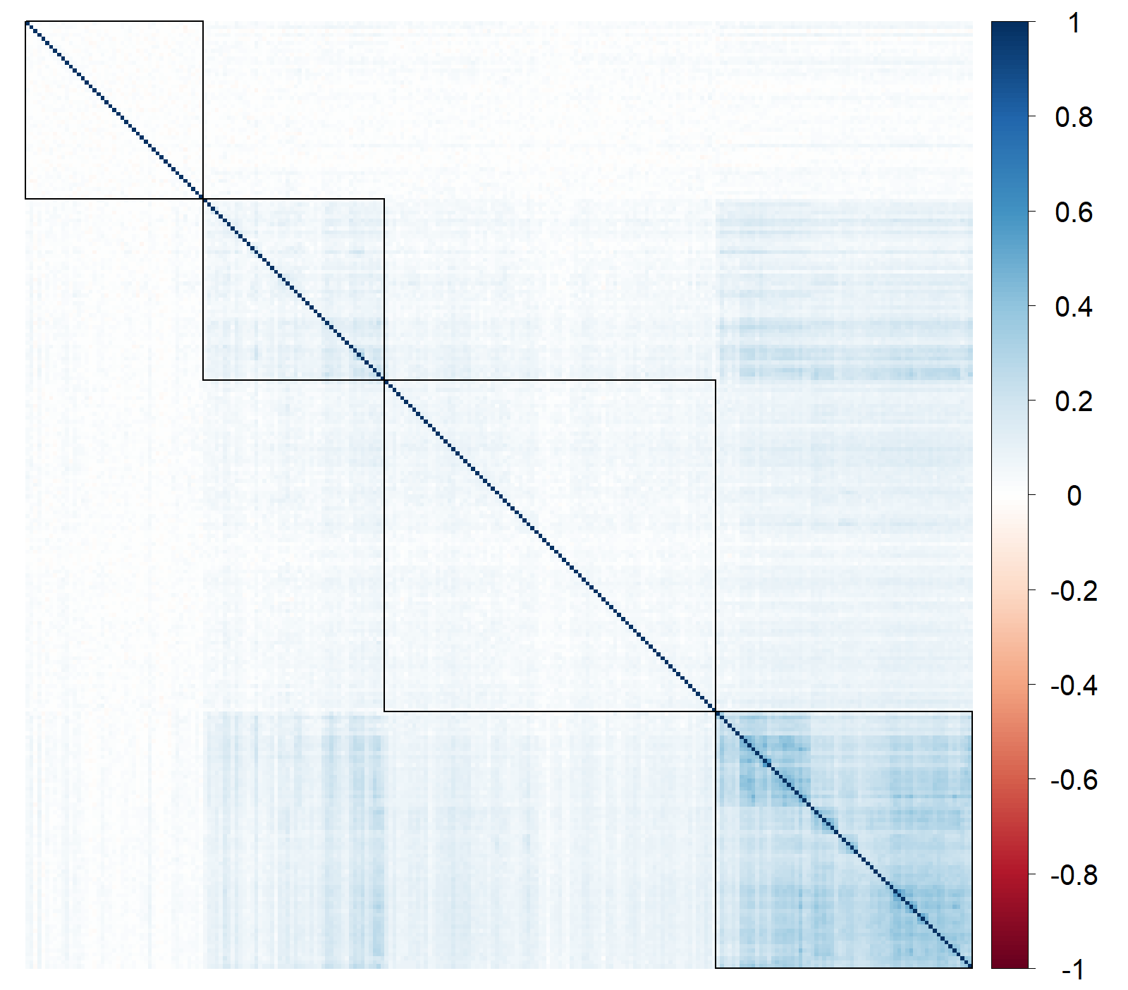
(b) clustered

Figure 1: Heatmap plots of the sample Kendall’s tau matrix computed on the daily log returns from 01 January 2007 until 14 January 2022 of all 240 portfolio stocks (whose list is available in Appendix B).

Note that after reordering of the variables by group, the corresponding Kendall’s tau matrix is block-structured with constant values in each of the off-diagonal blocks. The interest in investigating this structural assumption originates from applications in stock return modeling. In this context, the clustering of the variables could for instance be considered as grouping companies by sector or economy. It then seems at least intuitive to assume that companies from different groups have correlations that depend only on the groups they are in, without making any assumptions on the correlations between companies from the same group.

This can be clearly see on Figure 1: in each of the off-diagonal blocks the Kendall’s tau is mostly homogeneous, but significant differences can be seen in the fourth diagonal block. Indeed, it gathers companies whose link to other groups is constant, but with different relationships inside the group. This may be explained by the presence of subgroups inside this fourth group, even if the relationship with variables from other groups do not seem to be related to these subgroup structures.

Obviously, the structural assumption is satisfied for any set of variables by using only groups of length $1$. Therefore, assuming larger groups will make the assumption more constraining. Indeed, in this framework, Kendall’s tau matrix depends on

$$\frac{1}{2}K(K-1)+\frac{1}{2}\sum_{k=1}^{K}\lvert\mathcal{G}_{k}\rvert(\lvert\mathcal{G}_{k}\rvert-1)$$

free parameters. For a dimension of $100$, assuming we can split into $K=10$ groups of equal size, this translates to a reduction by factor of 10 of the number of free parameters to estimate (from $4950$ to $495$). Such a reduction suggests that the use of appropriate estimators can lead to significant estimation improvements.

Note that [28] proposed a similar model with a more restrictive version of Assumption A1, the Partial Exchangeability Assumption, by assuming that the variables could be partitioned into $K$ clusters with exchangeable dependence.

Assumption A2 (Partial Exchangeability Assumption).

For $j\in\{1,\ldots,p\}$, let $U_{j}=F_{j}\left(X_{j}\right)$, where $F_{j}$ is the cumulative distribution function of $X_{j}$, and $C$ be the copula of ${\mathbf{X}}$. For any partition $\mathcal{G}=\left\{\mathcal{G}_{1},\ldots,G_{K}\right\}$ of $\{1,\ldots,p\}$, let $\pi(G)$ be the set of permutations $\pi$ of $\{1,\ldots,p\}$ such that for all $j\in\{1,\ldots,p\}$ and all $k\in\{1,\ldots,K\}$, $\pi(j)\in\mathcal{G}_{k}$ if and only if $j\in\mathcal{G}_{k}$.

A partition $\mathcal{G}=\left\{\mathcal{G}_{1},\ldots,G_{K}\right\}$ satisfies the Partial Exchangeability Assumption if for any $u_{1},\ldots,u_{p}\in[0,1]$ and any permutation $\pi\in\pi(G)$, one has

$$C\left(u_{1},\ldots,u_{p}\right)=C\left(u_{\pi(1)},\ldots,u_{\pi(p)}\right)$$

or, equivalently, $\left(U_{1},\ldots,U_{p}\right)\stackrel{{\scriptstyle law}}{{=}}\left(U_{\pi(1)},\ldots,U_{\pi(p)}\right)$.

Note that the Partial Exchangeability Assumption imposes restrictions on the underlying copula, whereas Assumption A1 only does so on the underlying Kendall’s tau matrix, making it a lot less restrictive. Further, under Assumption A2, Kendall’s tau matrix is fully block-structured including constant diagonal blocks as well, after reordering of the variables. In contrast to [28], we are more interested in a model where we do not consider partial exchangeability nor constant interdependence of marginal variables within the same cluster. Particularly in view of the aforementioned application of stock returns, the Partial Exchangeability Assumption seems quite restrictive and a model without partial exchangeability in which companies from the same cluster have different mutual dependence is more plausible (see Figure 1). For these reasons, we opt for a more flexible variant of this model.

2.2 Consequences of the block structure on the correlation matrix

As explained in [20, Chapter 3], if ${\mathbf{X}}$ follows a multivariate Gaussian distribution with exchangeable dependence and correlation $\rho\in(-1,1)$, then $\mathrm{Corr}({\mathbf{X}})$ is positive definite if and only if $\rho>-1/(p-1)$. In terms of Kendall’s tau, this constraint translates as $\tau>-(2/\pi)\mathrm{Arcsin}(1/(p-1))$. Assumption A1 is weaker than exchangeable dependence, and even in the Gaussian setting with two groups of variables, it allows for arbitrary negative correlation in the off-diagonal block.

Proposition 1.

Let $b_{1},b_{2}\geq 2$ be integers. Let $\rho_{1},\rho_{2},\rho_{3}\in(-1,1)$, and define the block matrix $M\in{\mathbb{R}}^{(b_{1}+b_{2})^{2}}$ with blocks of size $b_{1}$ and $b_{2}$ by

$$M:=\left(\begin{array}[]{cc}I+\rho_{1}J&\rho_{3}{\bf 1}\\ \rho_{3}{\bf 1}&I+\rho_{2}J\end{array}\right),$$

where $I$ is the identity matrix and $J={\bf 1}-I$ is the matrix with $1$ at each off-diagonal entry and $0$ on the diagonal. Then $M$ is positive definite if and only if

$$\Big{(}\big{(}b_{2}b_{1}-b_{1}-b_{2}+1\big{)}\rho_{2}+b_{1}-1\Big{)}\rho_{1}-b_{1}b_{2}\rho_{3}^{2}+(b_{2}-1)\rho_{2}+1>0.$$ (1)

Furthermore, this inequality is satisfied as soon as

$$\left\{\begin{array}[]{l}\rho_{1}>\dfrac{b_{1}b_{2}\rho_{3}^{2}-(b_{2}-1)\rho_{2}-1}{\left(b_{1}b_{2}-b_{1}-b_{2}+1\right)\rho_{2}+b_{1}-1},\\ \rho_{2}>-\dfrac{b_{1}-1}{b_{1}b_{2}-b_{1}-b_{2}+1}.\end{array}\right.$$

This result is proved in Section A.1. We can remark that, the constraint (1) is always satisfied as soon as

$$\rho_{1}\rho_{2}\geq\rho_{3}^{2},$$ (2)

i.e. the absolute value of $\rho_{3}$ has to be smaller than the geometric mean of $\rho_{1}$ and $\rho_{2}$. Furthermore, in the high-dimensional setting where $b_{1},b_{2}\to+\infty$ and $\rho_{1},\rho_{2}$ are fixed and positive, (1) actually becomes equivalent to the simplified constraint (2). Note that (1) allows for situations where $\rho_{3}$ is arbitrarily close to $-1$, for any choice of block sizes. This is possible, for example, by setting $\rho_{1}=\rho_{2}=|\rho_{3}|$. Concretely, if all variables of one group have a high correlation with all variables of the second group, then in each group the intragroup correlation should be high. Such a result translates directly for Kendall’s tau matrix by using the relationship $\tau=(2/\pi)\mathrm{Arcsin}(\rho)$, allowing for Kendall’s tau matrix with arbitrary entries in the off-diagonal blocks.

Rather surprisingly, as soon as the group sizes $b_{1}$ and $b_{2}$ are large enough, they don’t appear anymore in the constraint (2). This phenomenon is in fact typical of block-structured matrices and will appear again in the performance of our estimators in the next sections. We now give a lower bound for the intergroup correlation in the setting where $K$ groups are present, with equal intergroup correlations. It is proved in Section A.1.

Proposition 2.

Let $K\geq 1$ and let $b_{1},\dots,b_{K}$ be positive integers. Let $\rho\in(-1,1)$, $\Sigma_{1},\dots,\Sigma_{K}$ be $K$ correlation matrices of size $b_{1},\dots b_{K}$ respectively and let $M\in{\mathbb{R}}^{(b_{1}+b_{2}+\dots+b_{K})^{2}}$ be the block matrix defined by

$$M:=\left(\begin{array}[]{cccc}\Sigma_{1}&\rho{\bf 1}&\cdots&\rho{\bf 1}\\ \rho{\bf 1}&\Sigma_{2}&\ddots&\vdots\\ \vdots&\ddots&\ddots&\rho{\bf 1}\\ \rho{\bf 1}&\cdots&\rho{\bf 1}&\Sigma_{K}\\ \end{array}\right)$$

Then

$$\inf\big{\{}\rho\in(-1,1):\exists\Sigma_{1},\dots,\Sigma_{K}\text{ such that }M\text{ is a correlation matrix }\big{\}}=\frac{-1}{K-1}.$$

Interestingly, this bound does not depend on the sizes of the blocks $b_{1},\dots,b_{K}$. This shows that, for such a matrix, the structure of each block does not have a strong influence on the possible choice of intergroup correlations. The constraint $\rho\geq-1/(p-1)$ for exchangeable correlation matrices becomes in this framework $\rho\geq-1/(K-1)$ for exchangeable intergroup dependence, suggesting that the number of blocks becomes the relevant dimension for this problem (instead of the number of variables). Nevertheless, the knowledge of the intragroup correlations matrices $\Sigma_{1},\dots,\Sigma_{K}$ will still constraint the range of possible values of $\rho$, as this was the case in Proposition 1 for the particular case $K=2$ and exchangeable dependence in each block.

2.3 Construction of estimators

In this section, we define estimators of the Kendall’s tau matrix ${\mathbf{T}}$ under Assumption A1 for some known partitions $\mathcal{G}$ of $\{1,\ldots,p\}$. Note that such partition can also be inferred from the data, see [28, 29]. First, let us define the group membership function $\kappa:\{1,\ldots,p\}\to\{1,\ldots,K\}$ by $\kappa(j):=k$ whenever $j\in\mathcal{G}_{k}$. Without loss of generality we assume that the ordering of variables is such that $j_{1}<j_{2}\Rightarrow\kappa(j_{1})\leq\kappa(j_{2})$, i.e. the variables are ordered by group and thus ${\mathbf{T}}$ has the proper block-structure. Naturally, we use the sample version of Kendall’s tau as a first step statistic, defined by

$$\widehat{\tau}_{1,2}:=\frac{2}{n(n-1)}\sum_{i_{1}<i_{2}}\operatorname{sign}\left(\left(X_{i_{1},1}-X_{i_{2},1}\right)\left(X_{i_{1},2}-X_{i_{2},2}\right)\right).$$ (3)

We denote the corresponding Kendall’s tau matrix estimator by $\widehat{{\mathbf{T}}}=\left[\widehat{\tau}_{j_{1},j_{2}}\right]_{p\times p}$, which serves as a first step estimator for obtaining a better estimator of the Kendall’s tau matrix. The sample Kendall’s tau matrix does not make any use of the underlying structure and will therefore be a rather naive tool in practice. Since we assume that the Kendall’s taus in each of the off-diagonal blocks are equal, the idea of averaging the pairwise sample Kendall’s tau follows naturally. Let us introduce the block estimator $\widehat{{\mathbf{T}}}^{B}$ that averages all sample Kendall’s taus within each of the off-diagonal blocks. Formally, we have

$$\widehat{{\mathbf{T}}}^{B}:=\left[\widehat{T}^{B}_{j_{1},j_{2}}\right]_{p\times p}=\begin{cases}\widehat{\tau}_{j_{1},j_{2}},&\text{if}\ \kappa(j_{1})=\kappa(j_{2})\\ \widehat{\tau}^{B}_{k_{1},k_{2}},&\text{for distinct}\ \kappa(j_{1})=k_{1}\text{ and }\kappa(j_{2})=k_{2},\end{cases}$$

where

$$\widehat{\tau}^{B}_{k_{1},k_{2}}:=\frac{1}{\lvert\mathcal{B}_{k_{1},k_{2}}\rvert}\sum_{(j_{1},j_{2})\in\mathcal{B}_{k_{1},k_{2}}}\widehat{\tau}_{j_{1},j_{2}},\quad\text{ and }\quad\mathcal{B}_{k_{1},k_{2}}:=\mathcal{G}_{k_{1}}\times\mathcal{G}_{k_{2}}.$$

Under the Partial Exchangeability Assumption, [28] showed that this estimator is asymptotically normal and optimal under the Mahalanobis distance. However, in terms of computational efficiency, the block estimator $\widehat{{\mathbf{T}}}^{B}$ does not show any improvement over the usual estimator $\widehat{{\mathbf{T}}}$, as both estimators require the computation of the usual Kendall’s tau between all pairs of variables anyway.

To reduce the computation time, we propose not averaging over all Kendall’s taus in the block but only over some of them. This would lead to computationally cheaper estimates. Naturally, the question arises over which elements then to average over. For this purpose, we introduce several estimators that average over different subsets of elements within each of the off-diagonal blocks.

We introduce two estimators that each average $N_{k_{1},k_{2}}\in\{1,\dots,\lvert\mathcal{G}_{k_{1}}\rvert\vee\lvert\mathcal{G}_{k_{2}}\rvert\}$ pairs per off-diagonal block $\mathcal{B}_{k_{1},k_{2}}$, so that we can compare estimators that either average pairs in the same row/column, or pairs on the diagonal. For averaging pairs on the diagonal, it is moreover required that $N_{k_{1},k_{2}}\leq\lvert\mathcal{G}_{k_{1}}\rvert\wedge\lvert\mathcal{G}_{k_{2}}\rvert$. The number of Kendall’s tau estimates is then reduced to scaling linearly with group size, which is a significant improvement over the previous quadratic growth. For distinct groups $k_{1},k_{2}\in\{1,\ldots,K\}$, we set

$$\widehat{\tau}^{R}_{k_{1},k_{2}} :=\frac{1}{N_{k_{1},k_{2}}}\sum_{(j_{1},j_{2})\in(\mathcal{B}_{k_{1},k_{2}})_{R}}\widehat{\tau}_{j_{1},j_{2}},$$

$$\widehat{\tau}^{D}_{k_{1},k_{2}} :=\frac{1}{N_{k_{1},k_{2}}}\sum_{(j_{1},j_{2})\in(\mathcal{B}_{k_{1},k_{2}})_{D}}\widehat{\tau}_{j_{1},j_{2}},$$

where $(\mathcal{B}_{k_{1},k_{2}})_{R}$ is the set of the $N_{k_{1},k_{2}}$ first pairs in the first line along the largest side of block $\mathcal{B}_{k_{1},k_{2}}$ and $(\mathcal{B}_{k_{1},k_{2}})_{D}$ is the set of the $N_{k_{1},k_{2}}$ first pairs on the first diagonal of the block. For example, if $N_{1,2}=3$, $\mathcal{G}_{1}=\{1,2,3,4\}$ and $\mathcal{G}_{2}=\{5,6,7\}$, then $(\mathcal{B}_{1,2})_{R}=\{(1,5),(2,5),(3,5)\}$ and $(\mathcal{B}_{1,2})_{D}=\{(1,5),(2,6),(3,7)\}$. Then, analogously to the definition of ${\mathbf{T}}^{B}$, we define the row estimator $\widehat{{\mathbf{T}}}^{R}$ and the diagonal estimator $\widehat{{\mathbf{T}}}^{D}$ as

$$\widehat{{\mathbf{T}}}^{R}:=\left[\widehat{T}^{R}_{j_{1},j_{2}}\right]_{p\times p}=\begin{cases}\widehat{\tau}_{j_{1},j_{2}},&\text{if}\ \kappa(j_{1})=\kappa(j_{2})\\ \widehat{\tau}^{R}_{k_{1},k_{2}},&\text{for distinct}\ \kappa(j_{1})=k_{1}\text{ and }\kappa(j_{2})=k_{2},\end{cases}$$

$$\widehat{{\mathbf{T}}}^{D}:=\left[\widehat{T}^{D}_{j_{1},j_{2}}\right]_{p\times p}=\begin{cases}\widehat{\tau}_{j_{1},j_{2}},&\text{if}\ \kappa(j_{1})=\kappa(j_{2})\\ \widehat{\tau}^{D}_{k_{1},k_{2}},&\text{for distinct}\ \kappa(j_{1})=k_{1}\text{ and }\kappa(j_{2})=k_{2}.\end{cases}$$

As such, for each of the off-diagonal blocks $\widehat{{\mathbf{T}}}^{R}$ averages only the pairs on the first line along the largest side, whereas $\widehat{{\mathbf{T}}}^{D}$ averages only the pairs along the first diagonal.

Lastly, we introduce the estimator that randomly selects pairs to average over per block. We denote the (deterministic) number of averaged pairs per block $\mathcal{B}_{k_{1},k_{2}}$ by $N_{k_{1},k_{2}}\in\{1,\dots,\lvert\mathcal{G}_{k_{1}}\rvert\times\lvert\mathcal{G}_{k_{2}}\rvert\}$ and the corresponding estimator by ${\mathbf{T}}^{U}$. The pairs are selected with uniform probability and without replacement. For distinct $k_{1},k_{2}\in\{1,\ldots,K\}$ we define

$$\widehat{\tau}^{U}_{k_{1},k_{2}}=\frac{1}{N_{k_{1},k_{2}}}\sum_{(j_{1},j_{2})\in\mathcal{B}_{k_{1},k_{2}}}W_{j_{1},j_{2}}\widehat{\tau}_{j_{1},j_{2}},$$

where $\mathbf{W}$ is a $p\times p$ matrix of random weights that selects $N_{k_{1},k_{2}}$ pairs per off-diagonal block $\mathcal{B}_{k_{1},k_{2}}$ with uniform probability and without replacement. $W_{j_{1},j_{2}}=1$ corresponds to selecting pair $(X_{j_{1}},X_{j_{2}})$ and $W_{j_{1},j_{2}}=0$ corresponds to passing over it. The corresponding matrix estimator is then given by

$$\widehat{{\mathbf{T}}}^{U}=\left[\widehat{T}^{U}_{j_{1},j_{2}}\right]=\begin{cases}\widehat{\tau}_{j_{1},j_{2}},&\text{if}\ \kappa(j_{1})=\kappa(j_{2})\\ \widehat{\tau}^{U}_{k_{1},k_{2}},&\text{for distinct}\ \kappa(j_{1})=k_{1}\text{ and }\kappa(j_{2})=k_{2}.\end{cases}$$

2.4 Comparison of their variances

Before we proceed with the main theoretical results on the estimators’ variances, let us introduce some auxiliary notations. For every distinct $k_{1},k_{2}\in\{1,\ldots,K\}$ we set

$$P_{k_{1},k_{2}} :=\mathbb{P}\left(\left(X_{j_{1},1}-X_{j_{1},2}\right)\left(X_{j_{2},1}-X_{j_{2},2}\right)>0\right),$$

where the pair $(j_{1},j_{2})$ lies within the block $\mathcal{B}_{k_{1},k_{2}}$. The quantity $P_{k_{1},k_{2}}$ is equal to the probability of concordance of the variables $X_{j_{1}}$ and $X_{j_{2}}$ and thus $\tau_{k_{1},k_{2}}=2P_{k_{1},k_{2}}-1$. As such, the structural assumption ensures that $P_{k_{1},k_{2}}$ is independent of the choice of pair $(j_{1},j_{2})\in\mathcal{B}_{k_{1},k_{2}}$. Alternatively we can write $P_{k_{1},k_{2}}$ in terms of the copula $C_{j_{1},j_{2}}$ of $(X_{j_{1}},X_{j_{2}})$ by

$$P_{k_{1},k_{2}}=2\int_{[0,1]^{2}}C_{j_{1},j_{2}}(u_{1},u_{2})\mathrm{d}C_{j_{1},j_{2}}(u_{1},u_{2}).$$

Further, for every pair $(j_{1},j_{2})\in\{1,\ldots,p\}^{2}$ we define

$$Q_{j_{1},j_{2}}:=\mathbb{P}\left(\left(X_{j_{1},1}-X_{j_{1},2}\right)\left(X_{j_{2},1}-X_{j_{2},2}\right)>0,\left(X_{j_{1},1}-X_{j_{1},3}\right)\left(X_{j_{2},1}-X_{j_{2},3}\right)>0\right).$$

Note that

$$Q_{j_{1},j_{2}}=\int_{[0,1]^{2}}(C_{j_{1},j_{2}}(u_{1},u_{2})+\bar{C}_{j_{1},j_{2}}(u_{1},u_{2}))^{2}\mathrm{d}C_{j_{1},j_{2}}(u_{1},u_{2}),$$ (4)

where $\bar{C}$ denotes the survival copula of variables $(X_{j_{1}},X_{j_{2}})$. For completeness, this expression is derived in Section A.2. Note that, for symmetric copulas, $\bar{C}(u_{1},u_{2})=C(1-u_{1},1-u_{2})$. Additionally, for all distinct $k_{1},k_{2}\in\{1,\ldots,K\}$ and for every $(j_{1},j_{2}),(j_{3},j_{4})\in\mathcal{B}_{k_{1},k_{2}}$ such that $\lvert\{j_{1},j_{2}\}\cap\{j_{3},j_{4}\}\rvert=1$ we define

$$R_{j_{1},j_{2},j_{3},j_{4}} :=\mathbb{P}\left(\left(X_{j_{1},1}-X_{j_{1},2}\right)\left(X_{j_{2},1}-X_{j_{2},2}\right)>0,\left(X_{j_{3},1}-X_{j_{3},2}\right)\left(X_{j_{4},1}-X_{j_{4},2}\right)>0\right)$$

$$S_{j_{1},j_{2},j_{3},j_{4}} :=\mathbb{P}\left(\left(X_{j_{1},1}-X_{j_{1},2}\right)\left(X_{j_{2},1}-X_{j_{2},2}\right)>0,\left(X_{j_{3},1}-X_{j_{3},3}\right)\left(X_{j_{4},1}-X_{j_{4},3}\right)>0\right).$$

and for every $(j_{1},j_{2}),(j_{3},j_{4})\in\mathcal{B}_{k_{1},k_{2}}$ such that $\{j_{1},j_{2}\}\cap\{j_{3},j_{4}\}=\emptyset$, we set

$$T_{j_{1},j_{2},j_{3},j_{4}} :=\mathbb{P}\left(\left(X_{j_{1},1}-X_{j_{1},2}\right)\left(X_{j_{2},1}-X_{j_{2},2}\right)>0,\left(X_{j_{3},1}-X_{j_{3},2}\right)\left(X_{j_{4},1}-X_{j_{4},2}\right)>0\right),$$

$$U_{j_{1},j_{2},j_{3},j_{4}} :=\mathbb{P}\left(\left(X_{j_{1},1}-X_{j_{1},2}\right)\left(X_{j_{2},1}-X_{j_{2},2}\right)>0,\left(X_{j_{3},1}-X_{j_{3},3}\right)\left(X_{j_{4},1}-X_{j_{4},3}\right)>0\right).$$

Note that these quantities $R,S,T,U$ can all be written as 8-dimensional integrals involving the copula of $X_{j_{1},j_{2},j_{3},j_{4}}$. $X_{(j_{1},j_{2},j_{3},j_{4})}$. As a consequence, they are all functions of the joint law ${\mathbb{P}}_{(j_{1},j_{2},j_{3},j_{4})}$ of the random vector ${\mathbf{X}}_{(j_{1},j_{2},j_{3},j_{4})}$, as well as $Q$. Note further that under Assumption A1, the quantities $Q_{j_{1},j_{2}}$, $R_{j_{1},j_{2},j_{3},j_{4}}$, $S_{j_{1},j_{2},j_{3},j_{4}}$, $T_{j_{1},j_{2},j_{3},j_{4}}$ and $U_{j_{1},j_{2},j_{3},j_{4}}$ are all depending on the choice of pairs within the off-diagonal block $\mathcal{B}_{k_{1},k_{2}}$.

Let $Q_{k_{1},k_{2}}^{B}$, $Q_{k_{1},k_{2}}^{R}$, $Q_{k_{1},k_{2}}^{D}$ denote the average among all $Q_{j_{1},j_{2}}$ of combinations of pairs within $\mathcal{B}_{k_{1},k_{2}}$, $(\mathcal{B}_{k_{1},k_{2}})_{R}$ and $(\mathcal{B}_{k_{1},k_{2}})_{D}$ respectively. Accordingly, we will denote the average among all $R_{j_{1},j_{2},j_{3},j_{4}}$ and all $S_{j_{1},j_{2},j_{3},j_{4}}$ of pairs within $\mathcal{B}_{k_{1},k_{2}}$ and $(\mathcal{B}_{k_{1},k_{2}})_{R}$ by respectively $R_{k_{1},k_{2}}^{B}$, $R_{k_{1},k_{2}}^{R}$ and $S_{k_{1},k_{2}}^{B}$, $S_{k_{1},k_{2}}^{R}$. Likewise, we set $T_{k_{1},k_{2}}^{B}$, $T_{k_{1},k_{2}}^{D}$ and $U_{k_{1},k_{2}}^{B}$, $U_{k_{1},k_{2}}^{D}$ for the averages among all $T_{j_{1},j_{2},j_{3},j_{4}}$ and all $U_{j_{1},j_{2},j_{3},j_{4}}$ of pairs within $\mathcal{B}_{k_{1},k_{2}}$ and $(\mathcal{B}_{k_{1},k_{2}})_{D}$.

Now that we have all auxiliary notations in place, let us start by showing that each of the estimators is in fact a U-statistic.

Lemma 3.

For distinct $k_{1},k_{2}\in\{1,\ldots,K\}$ and all $(j_{1},j_{2})\in\mathcal{B}_{k_{1},k_{2}}$, the estimators $\widehat{\tau}_{j_{1},j_{2}}$, $\widehat{\tau}_{k_{1},k_{2}}^{B},\widehat{\tau}^{R}_{k_{1},k_{2}},\widehat{\tau}^{D}_{k_{1},k_{2}}$ and $\widehat{\tau}^{U}_{k_{1},k_{2}}$ are all second order U-statistics.

This lemma is proved in Section A.3. From Lemma 3 and the fact that $\mathbb{E}\left[g^{*}\left((X_{j_{1}},X_{j_{2}})_{i_{1}},(X_{j_{1}},X_{j_{2}})_{i_{2}}\right)\right]=\tau_{k_{1},k_{2}}$ when $(j_{1},j_{2})\in\mathcal{B}_{k_{1},k_{2}}$, it follows that $\widehat{{\mathbf{T}}}$, $\widehat{{\mathbf{T}}}^{B}$, $\widehat{{\mathbf{T}}}^{R}$, $\widehat{{\mathbf{T}}}^{D}$ and $\widehat{{\mathbf{T}}}^{U}$ are all unbiased estimators of the Kendall’s tau matrix. The finite sample variances are given in the following theorem, proved in Section A.4.

Theorem 4.

Under Assumption A1, for distinct $k_{1},k_{2}\in\{1,\ldots,K\}$ and all $(j_{1},j_{2})\in\mathcal{B}_{k_{1},k_{2}}$, the variances of $\widehat{\tau}_{j_{1},j_{2}}$, $\widehat{\tau}_{k_{1},k_{2}}^{B},\widehat{\tau}^{R}_{k_{1},k_{2}},\widehat{\tau}^{D}_{k_{1},k_{2}}$ and $\widehat{\tau}^{U}_{k_{1},k_{2}}$ are given by

• $$\mathbb{V}\mathrm{ar}\left[\widehat{\tau}_{j_{1},j_{2}}\right] =\frac{8}{n(n-1)}\Big{(}P_{k_{1},k_{2}}-P_{k_{1},k_{2}}^{2}+2(n-2)\big{(}Q_{j_{1},j_{2}}-P_{k_{1},k_{2}}^{2}\big{)}\Big{)},$$

• $$\mathbb{V}\mathrm{ar}\left[\widehat{\tau}^{B}_{k_{1},k_{2}}\right] =\frac{8}{\lvert\mathcal{B}_{k_{1},k_{2}}\rvert n(n-1)}\bigg{(}P_{k_{1},k_{2}}-P^{2}_{k_{1},k_{2}}+\big{(}\lvert\mathcal{G}_{k_{1}}\rvert-1\big{)}\big{(}\lvert\mathcal{G}_{k_{2}}\rvert-1\big{)}\big{(}T_{k_{1},k_{2}}^{B}-P^{2}_{k_{1},k_{2}}\big{)}$$

  $$\hskip 152.0002pt+\big{(}\lvert\mathcal{G}_{k_{1}}\rvert+\lvert\mathcal{G}_{k_{2}}\rvert-2\big{)}\big{(}R_{k_{1},k_{2}}^{B}-P^{2}_{k_{1},k_{2}}\big{)}$$

  $$\hskip 80.00012pt+2(n-2)\Big{(}Q_{k_{1},k_{2}}^{B}-P^{2}_{k_{1},k_{2}}+\big{(}\lvert\mathcal{G}_{k_{1}}\rvert-1\big{)}\big{(}\lvert\mathcal{G}_{k_{2}}\rvert-1\big{)}\big{(}U_{k_{1},k_{2}}^{B}-P^{2}_{k_{1},k_{2}}\big{)}$$

  $$\hskip 197.00026pt+\big{(}\lvert\mathcal{G}_{k_{1}}\rvert+\lvert\mathcal{G}_{k_{2}}\rvert-2\big{)}\big{(}S_{k_{1},k_{2}}^{B}-P^{2}_{k_{1},k_{2}}\big{)}\Big{)}\bigg{)},$$

• $$\mathbb{V}\mathrm{ar}\left[\widehat{\tau}^{R}_{k_{1},k_{2}}\right]=\frac{8}{N_{k_{1},k_{2}}n(n-1)} \bigg{(}P_{k_{1},k_{2}}-P^{2}_{k_{1},k_{2}}+\big{(}N_{k_{1},k_{2}}-1\big{)}\big{(}R_{k_{1},k_{2}}^{R}-P^{2}_{k_{1},k_{2}}\big{)}$$

  $$+2(n-2)\Big{(}Q_{k_{1},k_{2}}^{R}-P^{2}_{k_{1},k_{2}}+\big{(}N_{k_{1},k_{2}}-1\big{)}(S_{k_{1},k_{2}}^{R}-P^{2}_{k_{1},k_{2}})\Big{)}\bigg{)},$$

• $$\mathbb{V}\mathrm{ar}\left[\widehat{\tau}^{D}_{k_{1},k_{2}}\right]=\frac{8}{N_{k_{1},k_{2}}n(n-1)} \bigg{(}P_{k_{1},k_{2}}-P^{2}_{k_{1},k_{2}}+\big{(}N_{k_{1},k_{2}}-1\big{)}\big{(}T_{k_{1},k_{2}}^{D}-P^{2}_{k_{1},k_{2}}\big{)}$$

  $$+2(n-2)\Big{(}Q_{k_{1},k_{2}}^{D}-P^{2}_{k_{1},k_{2}}+\big{(}N_{k_{1},k_{2}}-1\big{)}\big{(}U_{k_{1},k_{2}}^{D}-P^{2}_{k_{1},k_{2}}\big{)}\Big{)}\bigg{)},$$

• $$\mathbb{V}\mathrm{ar}\left[\widehat{\tau}^{U}_{k_{1},k_{2}}\right] =\frac{8}{N_{k_{1},k_{2}}n(n-1)}\Bigg{(}P_{k_{1},k_{2}}-P^{2}_{k_{1},k_{2}}+\frac{N_{k_{1},k_{2}}-1}{\lvert\mathcal{B}_{k_{1},k_{2}}\rvert-1}\Big{(}\big{(}\lvert\mathcal{G}_{k_{1}}\rvert-1\big{)}\big{(}\lvert\mathcal{G}_{k_{2}}\rvert-1\big{)}\big{(}T_{k_{1},k_{2}}^{B}-P^{2}_{k_{1},k_{2}}\big{)}$$

  $$\hskip 210.00032pt+\big{(}\lvert\mathcal{G}_{k_{1}}\rvert+\lvert\mathcal{G}_{k_{2}}\rvert-2\big{)}\big{(}R_{k_{1},k_{2}}^{B}-P^{2}_{k_{1},k_{2}}\big{)}\Big{)}$$

  $$\hskip 40.00006pt+2(n-2)\bigg{(}Q_{k_{1},k_{2}}^{B}-P^{2}_{k_{1},k_{2}}+\frac{N_{k_{1},k_{2}}-1}{\lvert\mathcal{B}_{k_{1},k_{2}}\rvert-1}\Big{(}\big{(}\lvert\mathcal{G}_{k_{1}}\rvert-1\big{)}\big{(}\lvert\mathcal{G}_{k_{2}}\rvert-1\big{)}\big{(}U_{k_{1},k_{2}}^{B}-P^{2}_{k_{1},k_{2}}\big{)}$$

  $$\hskip 210.00032pt+\big{(}\lvert\mathcal{G}_{k_{1}}\rvert+\lvert\mathcal{G}_{k_{2}}\rvert-2\big{)}\big{(}S_{k_{1},k_{2}}^{B}-P^{2}_{k_{1},k_{2}}\big{)}\Big{)}\bigg{)}\Bigg{)}.$$

This theorem is proved in Section A.4. Note that the variance of the sample Kendall’s tau estimator $\widehat{\tau}_{j_{1},j_{2}}$ is already known, see e.g. [15].

Remark 5.

If the stronger Assumption A2 holds, all quantities $Q_{j_{1},j_{2}}$, $R_{j_{1},j_{2},j_{3},j_{4}}$, $S_{j_{1},j_{2},j_{3},j_{4}}$, $T_{j_{1},j_{2},j_{3},j_{4}}$ and $U_{j_{1},j_{2},j_{3},j_{4}}$ are independent of the choice of pairs $(j_{1},j_{2}),(j_{3},j_{4})\in\mathcal{B}_{k_{1},k_{2}}$ for every distinct $k_{1},k_{2}\in\{1,\ldots,K\}$. It then follows that $Q^{B}_{k_{1},k_{2}}=Q^{R}_{k_{1},k_{2}}=Q^{D}_{k_{1},k_{2}}=Q_{i,j}$ and the same equality holds for quantities $R,S,T$ and $U$.

Corollary 6.

Under Assumption A1, for distinct $k_{1},k_{2}$ and all $(j_{1},j_{2})\in\mathcal{B}_{k_{1},k_{2}}$, it holds that as $n\to\infty$

$$n^{1/2}\left(\widehat{\tau}_{k_{1},k_{2}}-\tau_{k_{1},k_{2}}\right)\stackrel{{\scriptstyle\textnormal{law}}}{{\longrightarrow}}\mathcal{N}\left(0,V_{k_{1},k_{2}}\right),$$

where $\widehat{\tau}_{k_{1},k_{2}}$ denotes any of the estimators $\widehat{\tau}_{j_{1},j_{2}}$, $\widehat{\tau}^{B}_{k_{1},k_{2}}$, $\widehat{\tau}^{R}_{k_{1},k_{2}}$, $\widehat{\tau}^{D}_{k_{1},k_{2}}$, $\widehat{\tau}^{U}_{k_{1},k_{2}}$, and the corresponding asymptotic variances $V_{k_{1},k_{2}}$ are respectively given by

$$V_{j_{1},j_{2}}\hskip 1.4pt=V_{j_{1},j_{2}}({\mathbb{P}}_{\mathbf{X}})\hskip 1.4pt :=16(Q_{j_{1},j_{2}}-P_{k_{1},k_{2}}^{2}),$$ (5)

$$V_{k_{1},k_{2}}^{B}=V_{k_{1},k_{2}}^{B}({\mathbb{P}}_{\mathbf{X}}) :=\frac{16}{\lvert\mathcal{B}_{k_{1},k_{2}}\rvert}\Big{(}Q_{k_{1},k_{2}}^{B}-P^{2}_{k_{1},k_{2}}+\big{(}\lvert\mathcal{G}_{k_{1}}\rvert-1\big{)}\big{(}\lvert\mathcal{G}_{k_{2}}\rvert-1\big{)}(U_{k_{1},k_{2}}^{B}-P^{2}_{k_{1},k_{2}})$$

$$\hskip 118.0002pt+\big{(}\lvert\mathcal{G}_{k_{1}}\rvert+\lvert\mathcal{G}_{k_{2}}\rvert-2\big{)}\big{(}S_{k_{1},k_{2}}^{B}-P^{2}_{k_{1},k_{2}}\big{)}\Big{)},$$ (6)

$$V_{k_{1},k_{2}}^{R}=V_{k_{1},k_{2}}^{R}({\mathbb{P}}_{\mathbf{X}}) :=\frac{16}{N_{k_{1},k_{2}}}\Big{(}Q_{k_{1},k_{2}}^{R}-P^{2}_{k_{1},k_{2}}+\left(N_{k_{1},k_{2}}-1\right)\big{(}S_{k_{1},k_{2}}^{R}-P^{2}_{k_{1},k_{2}}\big{)}\Big{)},$$ (7)

$$V_{k_{1},k_{2}}^{D}=V_{k_{1},k_{2}}^{D}({\mathbb{P}}_{\mathbf{X}}) :=\frac{16}{N_{k_{1},k_{2}}}\Big{(}Q_{k_{1},k_{2}}^{D}-P^{2}_{k_{1},k_{2}}+\big{(}N_{k_{1},k_{2}}-1\big{)}\big{(}U_{k_{1},k_{2}}^{D}-P^{2}_{k_{1},k_{2}}\big{)}\Big{)},$$ (8)

$$V_{k_{1},k_{2}}^{U}=V_{k_{1},k_{2}}^{U}({\mathbb{P}}_{\mathbf{X}}) :=\frac{16}{N_{k_{1},k_{2}}}\bigg{(}Q_{k_{1},k_{2}}^{B}-P^{2}_{k_{1},k_{2}}+\frac{N_{k_{1},k_{2}}-1}{\lvert\mathcal{B}_{k_{1},k_{2}}\rvert-1}\Big{(}\big{(}\lvert\mathcal{G}_{k_{1}}\rvert-1\big{)}\big{(}\lvert\mathcal{G}_{k_{2}}\rvert-1\big{)}\big{(}U_{k_{1},k_{2}}^{B}-P^{2}_{k_{1},k_{2}}\big{)}$$

$$\hskip 160.00024pt+\big{(}\lvert\mathcal{G}_{k_{1}}\rvert+\lvert\mathcal{G}_{k_{2}}\rvert-2\big{)}\big{(}S_{k_{1},k_{2}}^{B}-P^{2}_{k_{1},k_{2}}\big{)}\Big{)}\bigg{)},$$ (9)

where ${\mathbb{P}}_{\mathbf{X}}$ denotes the law of the random vector $\mathbf{X}$. This can straightforwardly be derived by combining Theorem A of [34, Section 5.5.1] and the computations of the corresponding $\zeta_{1}$’s in the proof of Theorem 4.

From the lengthy expressions in Theorem 4 we can derive the asymptotic variances in the setting where $n,\lvert\mathcal{G}_{k_{1}}\rvert,\lvert\mathcal{G}_{k_{2}}\rvert,N_{k_{1},k_{2}}\to+\infty$.

Corollary 7.

Under Assumption A1, as $n,\lvert\mathcal{G}_{k_{1}}\rvert,\lvert\mathcal{G}_{k_{2}}\rvert,N_{k_{1},k_{2}}\to+\infty$, we have the following equivalents

• $\displaystyle\mathbb{V}\mathrm{ar}\left[\widehat{\tau}_{j_{1},j_{2}}\right]\sim\frac{16}{n}\left(Q_{j_{1},j_{2}}-P_{k_{1},k_{2}}^{2}\right)=\frac{1}{n}\times V_{j_{1},j_{2}}({\mathbb{P}}_{\mathbf{X}}),$

• $\displaystyle\mathbb{V}\mathrm{ar}\left[\widehat{\tau}^{B}_{k_{1},k_{2}}\right]\sim\frac{16}{n}\left(U_{k_{1},k_{2}}^{B}-P_{k_{1},k_{2}}^{2}\right)=\frac{1}{n}\times{\lim_{\lvert\mathcal{G}_{k_{1}}\rvert,\lvert\mathcal{G}_{k_{2}}\rvert\to+\infty}}V_{k_{1},k_{2}}^{B}({\mathbb{P}}_{\mathbf{X}}),$

• $\displaystyle\mathbb{V}\mathrm{ar}\left[\widehat{\tau}^{R}_{k_{1},k_{2}}\right]\sim\frac{16}{n}\left(S_{k_{1},k_{2}}^{R}-P_{k_{1},k_{2}}^{2}\right)=\frac{1}{n}\times{\lim_{N_{k_{1},k_{2}}\to+\infty}}V_{k_{1},k_{2}}^{R}({\mathbb{P}}_{\mathbf{X}}),$

• $\displaystyle\mathbb{V}\mathrm{ar}\left[\widehat{\tau}^{D}_{k_{1},k_{2}}\right]\sim\frac{16}{n}\left(U_{k_{1},k_{2}}^{D}-P_{k_{1},k_{2}}^{2}\right)=\frac{1}{n}\times{\lim_{N_{k_{1},k_{2}}\to+\infty}}V_{k_{1},k_{2}}^{D}({\mathbb{P}}_{\mathbf{X}}),$

• $\displaystyle\mathbb{V}\mathrm{ar}\left[\widehat{\tau}^{U}_{k_{1},k_{2}}\right]\sim\frac{16}{n}\left(U_{k_{1},k_{2}}^{B}-P_{k_{1},k_{2}}^{2}\right)=\frac{1}{n}\times{\lim_{\lvert\mathcal{G}_{k_{1}}\rvert,\lvert\mathcal{G}_{k_{2}}\rvert,N_{k_{1},k_{2}}\to+\infty}}V_{k_{1},k_{2}}^{U}({\mathbb{P}}_{\mathbf{X}}),$

assuming that $U_{k_{1},k_{2}}^{B},U_{k_{1},k_{2}}^{D},S_{k_{1},k_{2}}^{R}$ are constant and strictly larger than $P_{k_{1},k_{2}}^{2}$. If this is not the case, the corresponding variances converges to $0$ at a rate faster than $O(1/n)$.

Surprisingly, note that the variances do not depend on the block dimensions as soon as they are large enough. This is also true if the block dimensions tends to the infinity at different rates. In the limit, the quality of the estimator will therefore not improve by averaging over additional elements in general. Note that this is coherent, since we do not assume the dependence to converge to $0$, which would correspond to some mixing assumption. Therefore, averaging must have only a limited effect, as in the simpler statistical model $Y_{i}=\theta+\epsilon_{i}$ where $\epsilon=(\epsilon_{1},\dots,\epsilon_{n})$ follows an exchangeable Normal distribution with correlation $\rho>0$. In this case, the average $\overline{Y}_{n}$ is inconsistent for estimating $\theta$ since $\mathbb{E}[(\overline{Y}_{n}-\theta)^{2}]=n^{-2}\sum_{i,j=1}^{n}\mathbb{E}[\epsilon_{i}\epsilon_{j}]=1/n+(n-1)\rho/n\to\rho$ as $n\to\infty$.

For large sample sizes, only the quantities $Q$, $S$ and $U$ determine the levels of variance. Whether the asymptotic variance contains either $S$ or $U$ is determined by which terms (corresponding to the overlapping and non-overlapping combinations of pairs) get the overhand in the summing of the proof of Theorem 4 when dimensions tend to infinity. For the diagonal, random and block estimators, the number of terms corresponding to non-overlapping combinations grow faster than the number of overlapping combinations. However, for the row estimator only pairs within the same row are averaged, and thus the limiting variance contains the quantity $S$ (instead of $U$). Furthermore, it should be noted that for every distinct $k_{1},k_{2}$ we have $U_{k_{1},k_{2}}^{B}\leq Q_{k_{1},k_{2}}^{B}$ and $S_{k_{1},k_{2}}^{R}\leq Q_{k_{1},k_{2}}^{R}$ with equality if and only if the Kendall’s taus within the diagonal blocks corresponding to $k_{1}$ and $k_{2}$ are equal to 1. This follows from the fact that averaging among several unbiased estimates reduces the total variance when compared to no averaging.

Open problem. It would seem natural from the definitions of $Q_{j_{1},j_{2}}$, $S_{j_{1},j_{2},j_{1},j_{3}}$ and $U_{j_{1},j_{2},j_{3},j_{4}}$ that

$$U_{j_{1},j_{2},j_{3},j_{4}}\leq S_{j_{1},j_{2},j_{1},j_{3}}\leq Q_{j_{1},j_{2}},$$ (10)

for all pairs $(j_{1},j_{2})$, $(j_{1},j_{3})$, $(j_{3},j_{4})$ such these quantities are all well defined, i.e. $(j_{1},j_{2})$, $(j_{1},j_{3})$, $(j_{3},j_{4})\in\mathcal{B}_{k_{1},k_{2}}$ such that $k_{1},k_{2}$ are distinct. The intuition behind this is the following: the probability that both pairs of observations $(1,2)$ and $(1,3)$ are concordant should be naturally greater if the corresponding pairs of variables $\{j_{1},j_{2}\}$ and $\{j_{3},j_{4}\}$ overlap (assuming some kind of positive dependence). If so, then the row estimator performs worse than the block, diagonal and random estimator. Empirically, we indeed observe that this is the case. However, a proof of this inequality seems very difficult, even under seemingly easy frameworks. For instance, even in the case of Gaussian copulas with constant correlation $r$, this would require the computation of involved integrals such as

$$\int_{-\infty}^{\infty}\int_{-\infty}^{\infty} {\mathrm{e}}^{-rx_{1}x_{2}-\frac{1}{2}x_{1}^{2}-\frac{1}{2}x_{2}^{2}}$$

$$\times\mathrm{erf}\left(x_{1}+x_{2}+a\right)\mathrm{erf}\left(x_{1}+x_{2}+b\right)\mathrm{erf}\left(x_{1}+x_{2}+c\right)\mathrm{erf}\left(x_{1}+x_{2}+d\right)\mathrm{d}x_{1}\mathrm{d}x_{2},$$

for some reals $a,b,c,d,r$, where $\mathrm{erf}$ is the Gauss error function. Using integration by part, a necessary condition would be the computation of the indefinite integral $\int\exp(-x^{2})\mathrm{erf}(\alpha+\beta x)\mathrm{d}x$ for $\alpha,\beta\in{\mathbb{R}}$. Except when $\alpha=\beta=0$, this integral does not appear in usual tables of integrals; the computer algebra system Maple was also unable to compute this integral and we conjecture that it cannot be expressed using standard functions.

Interestingly, the block estimator, the diagonal estimator and the random estimator perform (almost) equally well in the limit, assuming that the averages $U^{B}$ and $U^{D}$ are not far apart. Hence, we can greatly reduce computation time by using either one of the diagonal or random estimator instead of the block estimator, while still maintaining a low asymptotic variance. This is summarized in the following corollary. Furthermore, we set additional conditions to derive an ordering of the three estimators.

Corollary 8.

Under Assumption A1 we have the following:

• Assume that the quantity $U$ does not depend on the choice of pairs within the off-diagonal block $\mathcal{B}_{k_{1},k_{2}}$. Then, the asymptotic variances of the block, diagonal and random estimators are equal:

  $${\lim_{\lvert\mathcal{G}_{k_{1}}\rvert,\lvert\mathcal{G}_{k_{2}}\rvert,n\to+\infty}}n\mathbb{V}\mathrm{ar}\left[\widehat{\tau}^{B}_{k_{1},k_{2}}\right] ={\lim_{\begin{subarray}{c}n\to+\infty\\ N_{k_{1},k_{2}}\to+\infty\end{subarray}}}n\mathbb{V}\mathrm{ar}\left[\widehat{\tau}^{D}_{k_{1},k_{2}}\right]$$

  $$={\lim_{\begin{subarray}{c}\lvert\mathcal{G}_{k_{1}}\rvert,\lvert\mathcal{G}_{k_{2}}\rvert,\\ n,N_{k_{1},k_{2}}\end{subarray}\to+\infty}}n\mathbb{V}\mathrm{ar}\left[\widehat{\tau}^{U}_{k_{1},k_{2}}\right]=U_{k_{1},k_{2}}-P_{k_{1},k_{2}}^{2}:=\sigma_{A}^{2}.$$

• Further, assume that quantities $Q$ and $S$ do not depend on the choice of pairs within $\mathcal{B}_{k_{1},k_{2}}$ and that $U<S<\frac{1}{2}Q+\frac{1}{2}U$. Then, there is a natural ordering between the estimators, given by:

  $$0 <{\lim_{\lvert\mathcal{G}_{k_{1}}\rvert,\lvert\mathcal{G}_{k_{2}}\rvert,n\to+\infty}}n\,\lvert\mathcal{G}_{k_{1}}\rvert\wedge\lvert\mathcal{G}_{k_{2}}\rvert\left(\mathbb{V}\mathrm{ar}\left[\widehat{\tau}^{B}_{k_{1},k_{2}}\right]-\sigma_{A}^{2}\right)$$

  $$<{\lim_{\begin{subarray}{c}n\to+\infty\\ N_{k_{1},k_{2}}\to+\infty\end{subarray}}}n\,N_{k_{1},k_{2}}\left(\mathbb{V}\mathrm{ar}\left[\widehat{\tau}^{D}_{k_{1},k_{2}}\right]-\sigma_{A}^{2}\right)<{\lim_{\begin{subarray}{c}\lvert\mathcal{G}_{k_{1}}\rvert,\lvert\mathcal{G}_{k_{2}}\rvert,\\ n,N_{k_{1},k_{2}}\end{subarray}\to+\infty}}n\,N_{k_{1},k_{2}}\left(\mathbb{V}\mathrm{ar}\left[\widehat{\tau}^{U}_{k_{1},k_{2}}\right]-\sigma_{A}^{2}\right),$$

• Assume, moreover, that quantities $R$ and $T$ do not depend on the choice of pairs within $\mathcal{B}_{k_{1},k_{2}}$ and that $T<R<\frac{1}{2}P+\frac{1}{2}T$. Then, there is a natural ordering for finite sample sizes and block dimensions, given by:

  $$\mathbb{V}\mathrm{ar}\left[\widehat{\tau}^{B}_{k_{1},k_{2}}\right]<\mathbb{V}\mathrm{ar}\left[\widehat{\tau}^{D}_{k_{1},k_{2}}\right]<\mathbb{V}\mathrm{ar}\left[\widehat{\tau}^{U}_{k_{1},k_{2}}\right],$$

  when $N_{k_{1},k_{2}}=\lvert\mathcal{G}_{k_{1}}\rvert\wedge\lvert\mathcal{G}_{k_{2}}\rvert$.

This corollary is proved in Section A.5. As a consequence of this result, under the above conditions the variance of the block estimator converges the fastest to the asymptotic variance. This is coherent with Theorem 1 of [28] which shows that under Assumption A2 the block averaging estimator is optimal with respect to the Mahalanobis distance. Furthermore, since the diagonal estimator averages solely over non-overlapping combinations, note that it should converge faster than that of the random estimator. Therefore, if computation costs are to be reduced, the diagonal estimator is preferable to both the random and the row estimator.

Lastly, we note that if only part of the row or diagonal is averaged, the asymptotic variances of the resulting estimators do not change. By doing so we can further lower computation times, but at the cost of attaining the limiting variances at slower rates. It therefore makes sense to choose $N_{k_{1},k_{2}}$ large enough to attain the asymptotic rates, but not too large to keep a low computation time.

3 Fast estimation of conditional Kendall’s tau matrix

We extend the aforementioned setting to the conditional setup, when a $d$-dimensional covariate ${\mathbf{Z}}$ is available taking values in $\mathcal{Z}\subset{\mathbb{R}}^{d}$. The objective is now to estimate the $p\times p$ conditional Kendall’s tau matrix ${\mathbf{T}}_{\mid{\mathbf{Z}}={\mathbf{z}}}=\left[\tau_{j_{1},j_{2}\mid{\mathbf{Z}}={\mathbf{z}}}\right]$. To this end, we study several kernel-based estimators of the pairwise conditional Kendall’s tau in Section 3.1. Then, in Section 3.2 we formalize the assumptions and construct the estimators adjusted for the conditional setup. Lastly, the main theoretical results on the estimators’ asymptotic variances are presented in Section 3.3.

3.1 Estimation of conditional Kendall’s tau

For construction of nonparametric estimates of the conditional Kendall’s tau, let us start by recalling the equivalent expressions of the conditional Kendall’s tau, following [7]:

$$\tau_{1,2\mid{\mathbf{Z}}={\mathbf{z}}} =\mathbb{P}\left(\left(X_{1,1}-X_{1,2}\right)\left(X_{2,1}-X_{2,2}\right)>0\mid{\mathbf{Z}}_{1}={\mathbf{Z}}_{2}={\mathbf{z}}\right)-\mathbb{P}\left(\left(X_{1,1}-X_{1,2}\right)\left(X_{2,1}-X_{2,2}\right)<0\mid{\mathbf{Z}}_{1}={\mathbf{Z}}_{2}={\mathbf{z}}\right)$$

$$=4\,\mathbb{P}\left(X_{1,1}<X_{1,2},X_{2,1}<X_{2,2}\mid{\mathbf{Z}}_{1}={\mathbf{Z}}_{2}={\mathbf{z}}\right)-1$$

$$=1-4\,\mathbb{P}\left(X_{1,1}<X_{1,2},X_{2,1}>X_{2,2}\mid{\mathbf{Z}}_{1}={\mathbf{Z}}_{2}={\mathbf{z}}\right),$$

Following the approach of [7], we introduce several kernel estimators of $\tau_{1,2\mid{\mathbf{Z}}={\mathbf{z}}}$ motivated by each of the equivalent definitions

$$\widehat{\tau}^{(1)}_{1,2\mid{\mathbf{Z}}={\mathbf{z}}} :=\sum_{i_{1}=1}^{n}\sum_{i_{2}=1}^{n}w_{i_{1},n}({\mathbf{z}})w_{i_{2},n}({\mathbf{z}})\bigg{(}\mathds{1}\left\{\left(X_{i_{1},1}-X_{i_{2},1}\right)\left(X_{2,i_{1}}-X_{i_{2},2}\right)>0\right\}$$

$$\hskip 130.0002pt-\mathds{1}\left\{\left(X_{i_{1},1}-X_{i_{2},1}\right)\left(X_{2,i_{1}}-X_{i_{2},2}\right)<0\right\}\bigg{)},$$

$$\widehat{\tau}^{(2)}_{1,2\mid{\mathbf{Z}}={\mathbf{z}}} :=4\sum_{i_{1}=1}^{n}\sum_{i_{2}=1}^{n}w_{i_{1},n}({\mathbf{z}})w_{i_{2},n}({\mathbf{z}})\mathds{1}\left\{X_{i_{1},1}<X_{i_{2},1},X_{2,i_{1}}<X_{i_{2},2}\right\}-1,$$

$$\widehat{\tau}^{(3)}_{1,2\mid{\mathbf{Z}}={\mathbf{z}}} :=1-4\sum_{i_{1}=1}^{n}\sum_{i_{2}=1}^{n}w_{i_{1},n}({\mathbf{z}})w_{i_{2},n}({\mathbf{z}})\mathds{1}\left\{X_{i_{1},1}<X_{i_{2},1},X_{2,i_{1}}>X_{i_{2},2}\right\},$$

with Nadaraya-Watson weights $w_{i,n}$ given by

$$w_{i,n}({\mathbf{z}}):=\frac{{\mathcal{K}}_{h}({\mathbf{Z}}_{i}-{\mathbf{z}})}{\sum_{k=1}^{n}{\mathcal{K}}_{h}({\mathbf{Z}}_{k}-{\mathbf{z}})},$$ (11)

for some kernel ${\mathcal{K}}$ on ${\mathbb{R}}^{d}$ and a bandwidth sequence $h=h(n)$ converging to zero as $n\to\infty$. Further, let us define

$$g_{1}((X_{1},X_{2})_{i_{1}},(X_{1},X_{2})_{i_{2}}) :=\mathds{1}\left(\left(X_{i_{1},1}-X_{i_{2},1}\right)\left(X_{i_{1},2}-X_{i_{2},2}\right)>0\right)-\mathds{1}\left(\left(X_{i_{1},1}-X_{i_{2},1}\right)\left(X_{i_{1},2}-X_{i_{2},2}\right)<0\right),$$

$$g_{2}((X_{1},X_{2})_{i_{1}},(X_{1},X_{2})_{i_{2}}) :=4\,\mathds{1}\left(X_{i_{1},1}<X_{i_{1},1},X_{i_{2},1}<X_{i_{2},1}\right)-1,$$

$$g_{3}((X_{1},X_{2})_{i_{1}},(X_{1},X_{2})_{i_{2}}) :=1-4\,\mathds{1}\left(X_{i_{1},1}<X_{i_{2},1},X_{i_{1},2}>X_{i_{2},2}\right).$$

Then $\widehat{\tau}^{(s)}_{1,2\mid{\mathbf{Z}}={\mathbf{z}}}$ is a smoothed estimator of $\tau_{1,2\mid{\mathbf{Z}}={\mathbf{z}}}=\mathbb{E}\left[g_{s}(\mathbf{X}_{i},\mathbf{X}_{j})\mid{\mathbf{Z}}_{1}={\mathbf{Z}}_{2}={\mathbf{z}}\right]$, for any choice of $s=1,2,3$. However, note that the terms for which $i_{1}=i_{2}$ are treated differently by each of the estimators. Consequently, the estimators $\widehat{\tau}^{(s)}_{1,2\mid{\mathbf{Z}}={\mathbf{z}}},$ $s=1,2,3$ all take values in different subsets of $[-1,1]$, as remarked in [7]. We therefore define a rescaled version taking values in $[-1,1]$ by

$$\widetilde{\tau}_{j_{1},j_{2}\mid{\mathbf{Z}}={\mathbf{z}}}:=\frac{\widehat{\tau}^{(1)}_{j_{1},j_{2}\mid{\mathbf{Z}}={\mathbf{z}}}}{1-s_{n}}=\frac{\widehat{\tau}^{(2)}_{j_{1},j_{2}\mid{\mathbf{Z}}={\mathbf{z}}}}{1-s_{n}}+\frac{s_{n}}{1-s_{n}}=\frac{\widehat{\tau}^{(3)}_{j_{1},j_{2}\mid{\mathbf{Z}}={\mathbf{z}}}}{1-s_{n}}-\frac{s_{n}}{1-s_{n}}.$$ (12)

where $s_{n}:=\sum_{i=1}^{n}w_{i,n}^{2}({\mathbf{z}}).$ Naturally, we prefer the rescaled version over the other estimators since it takes values in the whole interval $[-1,1]$.

3.2 The conditional setup

In the conditional setup, we need adapted versions of the structural assumption as well as adapted versions of each of the estimators. We adapt the structural assumption by assuming that the underlying structural pattern applies to the conditional Kendall’s tau matrix for any value of the covariate ${\mathbf{Z}}$. We formalize this in the following assumption.

Assumption A3 (Conditional Structural Assumption).

There exists $K>0$ and a partition $\mathcal{G}=\{\mathcal{G}_{1},\dots,\mathcal{G}_{K}\}$ of $\{1,\dots,p\}$, such that for all distinct $k_{1},k_{2}\in\{1,\dots,K\}$ and all ${\mathbf{z}}\in\mathcal{Z}$,

$$\left[{\mathbf{T}}_{\mid{\mathbf{Z}}={\mathbf{z}}}\right]_{\mathcal{B}_{k_{1},k_{2}}}=\tau_{k_{1},k_{2}\mid{\mathbf{Z}}={\mathbf{z}}}\cdot{\bf 1}$$

for some $\tau_{k_{1},k_{2}\mid{\mathbf{Z}}={\mathbf{z}}}\in[-1,1]$, where $\mathcal{B}_{k_{1},k_{2}}:=\left\{\left(j_{1},j_{2}\right)\in\left(\mathcal{G}_{k_{1}}\times\mathcal{G}_{k_{2}}\right)\right\}$.

In terms of stock return modeling, Assumption A3 has the following interpretation: conditionally on a given market state or portfolio movement, the stocks of companies from different sectors/countries have equal rank correlations with every other pair from the respective groups. This could for instance be used for the computation of conditional risk measures. Note that we also assume that the blocks do not change with ${\mathbf{z}}$, which seems reasonable in our perspective of groups chosen from sectors or countries. For any fixed ${\mathbf{z}}\in\mathcal{Z}$, the number of free parameters is again reduced from $\frac{1}{2}p(p-1)$ to

$$\frac{1}{2}K(K-1)+\frac{1}{2}\sum_{k=1}^{K}\lvert\mathcal{G}_{k}\rvert(\lvert\mathcal{G}_{k}\rvert-1),$$

allowing for an improved estimation based on the averaging principle. Note that here the free parameters are functions of ${\mathbf{z}}$ and therefore live in an infinite-dimensional space, contrary to the previous section where each parameter was a real number.

Let us denote the naive (unaveraged) conditional Kendall’s tau matrix estimator as $\widehat{{\mathbf{T}}}_{\mid{\mathbf{Z}}={\mathbf{z}}}=\left[\widetilde{\tau}_{j_{1},j_{2}\mid{\mathbf{Z}}={\mathbf{z}}}\right]_{p\times p}$ with $\widetilde{\tau}_{j_{1},j_{2}\mid{\mathbf{Z}}={\mathbf{z}}}$ as in (12). As in the unconditional framework that was studied previously, we define conditional versions of the averaging estimators by

$$\widehat{\tau}^{B}_{k_{1},k_{2}\mid{\mathbf{Z}}={\mathbf{z}}} :=\frac{1}{\lvert\mathcal{B}_{k_{1},k_{2}}\rvert}\sum_{(j_{1},j_{2})\in\mathcal{B}_{k_{1},k_{2}}}\widetilde{\tau}_{j_{1},j_{2}\mid{\mathbf{Z}}={\mathbf{z}}},\qquad\hskip 6.00006pt\widehat{\tau}^{R}_{k_{1},k_{2}\mid{\mathbf{Z}}={\mathbf{z}}}:=\frac{1}{N_{k_{1},k_{2}}}\sum_{(j_{1},j_{2})\in(\mathcal{B}_{k_{1},k_{2}})_{R}}\widetilde{\tau}_{j_{1},j_{2}\mid{\mathbf{Z}}={\mathbf{z}}},$$

$$\widehat{\tau}^{D}_{k_{1},k_{2}\mid{\mathbf{Z}}={\mathbf{z}}} :=\frac{1}{N_{k_{1},k_{2}}}\sum_{(j_{1},j_{2})\in(\mathcal{B}_{k_{1},k_{2}})_{D}}\widetilde{\tau}_{j_{1},j_{2}\mid{\mathbf{Z}}={\mathbf{z}}},\qquad\widehat{\tau}^{U}_{k_{1},k_{2}\mid{\mathbf{Z}}={\mathbf{z}}}:=\frac{1}{N_{k_{1},k_{2}}}\sum_{(j_{1},j_{2})\in\mathcal{B}_{k_{1},k_{2}}}W_{j_{1},j_{2}}\widetilde{\tau}_{j_{1},j_{2}\mid{\mathbf{Z}}={\mathbf{z}}},$$

using the same notations $\mathcal{B}_{k_{1},k_{2}},(\mathcal{B}_{k_{1},k_{2}})_{R},(\mathcal{B}_{k_{1},k_{2}})_{D},N_{k_{1},k_{2}}$ and $\mathbf{W}$ as before. The corresponding conditional Kendall’s tau matrix estimators are respectively denoted by $\widehat{{\mathbf{T}}}^{B}_{\mid{\mathbf{Z}}={\mathbf{z}}}$, $\widehat{{\mathbf{T}}}^{R}_{\mid{\mathbf{Z}}={\mathbf{z}}}$, $\widehat{{\mathbf{T}}}^{D}_{\mid{\mathbf{Z}}={\mathbf{z}}}$ and $\widehat{{\mathbf{T}}}^{U}_{\mid{\mathbf{Z}}={\mathbf{z}}}$.

Next, let us define auxiliary notations $P,Q,S$ and $U$ for the conditional setup. Under Assumption A3, we define the conditional version of $P_{k_{1},k_{2}}$ for each distinct $k_{1},k_{2}\in\{1,\ldots,K\}$ and all ${\mathbf{z}}\in\mathcal{Z}$ as

$$P_{k_{1},k_{2}\mid{\mathbf{Z}}={\mathbf{z}}} :=\mathbb{P}\left(\left(X_{j_{1},1}-X_{j_{1},2}\right)\left(X_{j_{2},1}-X_{j_{2},2}\right)>0\mid{\mathbf{Z}}_{1}={\mathbf{Z}}_{2}={\mathbf{z}}\right),$$

where $(j_{1},j_{2})$ is a pair in the block $\mathcal{B}_{k_{1},k_{2}}$. Note that Assumption A3 ensures that $P_{k_{1},k_{2}\mid{\mathbf{Z}}={\mathbf{z}}}$ is independent of the choice of the pair $(j_{1},j_{2})\in\mathcal{B}_{k_{1},k_{2}}$. Alternatively, we can write $P_{k_{1},k_{2}\mid{\mathbf{Z}}={\mathbf{z}}}$ in terms of the conditional copula $C_{j_{1},j_{2}\mid{\mathbf{Z}}={\mathbf{z}}}$ (defined as the copula of the corresponding conditional distribution, see [13, 27]) of $(X_{j_{1}},X_{j_{2}})$ by

$$P_{k_{1},k_{2}\mid{\mathbf{Z}}={\mathbf{z}}}=2\int_{[0,1]^{2}}C_{j_{1},j_{2}\mid{\mathbf{Z}}={\mathbf{z}}}(u_{1},u_{2})\mathrm{d}C_{j_{1},j_{2}\mid{\mathbf{Z}}={\mathbf{z}}}(u_{1},u_{2}).$$

Let the conditional version of $Q_{j_{1},j_{2}}$ for every $(j_{1},j_{2})\in\{1,\ldots,p\}^{2}$ and all ${\mathbf{z}}\in\mathcal{Z}$ be given by

$$Q_{j_{1},j_{2}\mid{\mathbf{Z}}={\mathbf{z}}}:=\mathbb{P}( \left(X_{j_{1},1}-X_{j_{1},2}\right)\left(X_{j_{2},1}-X_{j_{2},2}\right)>0,$$

$$\left(X_{j_{1},1}-X_{j_{1},3}\right)\left(X_{j_{2},1}-X_{j_{2},3}\right)>0\mid{\mathbf{Z}}_{1}={\mathbf{Z}}_{2}={\mathbf{z}}),$$

or, alternatively, in terms of conditional copulas

$$Q_{j_{1},j_{2}\mid{\mathbf{Z}}={\mathbf{z}}}=\int_{[0,1]^{2}}\left(C_{j_{1},j_{2}\mid{\mathbf{Z}}={\mathbf{z}}}(u_{1},u_{2})+\bar{C}_{{\mathbf{Z}}={\mathbf{Z}}}(u_{1},u_{2})\right)\mathrm{d}C_{j_{1},j_{2}{\mathbf{Z}}={\mathbf{Z}}}(u_{1},u_{2}),$$

where $\bar{C}_{j_{1},j_{2}\mid{\mathbf{Z}}={\mathbf{Z}}}$ denotes the survival copula of the variables $(X_{j_{1}},X_{j_{2}})$ conditionally on ${\mathbf{Z}}={\mathbf{z}}$. For all ${\mathbf{z}}\in\mathcal{Z}$, for all distinct $k_{1},k_{2}\in\{1,\ldots,K\}$ and for all $(j_{1},j_{2}),(j_{3},j_{4})\in\mathcal{B}_{k_{1},k_{2}}$ such that $\lvert\{j_{1},j_{2}\}\cap\{j_{3},j_{4}\}\rvert=1$, we define

$$S_{j_{1},j_{2},j_{3},j_{4}\mid{\mathbf{Z}}={\mathbf{z}}}:=\mathbb{P}( \left(X_{j_{1},1}-X_{j_{1},2}\right)\left(X_{j_{2},1}-X_{j_{2},2}\right)>0,$$

$$\left(X_{j_{3},1}-X_{j_{3},3}\right)\left(X_{j_{4},1}-X_{j_{4},3}\right)>0\mid{\mathbf{Z}}_{1}={\mathbf{Z}}_{2}={\mathbf{Z}}_{3}={\mathbf{z}}),$$

and for every $(j_{1},j_{2}),(j_{3},j_{4})\in\mathcal{B}_{k_{1},k_{2}}$ such that $\{j_{1},j_{2}\}\cap\{j_{3},j_{4}\}=\emptyset$, we define

$$U_{j_{1},j_{2},j_{3},j_{4}\mid{\mathbf{Z}}={\mathbf{z}}}:=\mathbb{P}( \left(X_{j_{1},1}-X_{j_{1},2}\right)\left(X_{j_{2},1}-X_{j_{2},2}\right)>0,$$

$$\left(X_{j_{3},1}-X_{j_{3},3}\right)\left(X_{j_{4},1}-X_{j_{4},3}\right)>0\mid{\mathbf{Z}}_{1}={\mathbf{Z}}_{2}={\mathbf{Z}}_{3}={\mathbf{z}}).$$

As before, the notations $Q^{B}$, $Q^{R}$ and $Q^{D}$ are used to denote the auxiliary quantities averaged over the whole block, row, or diagonal, respectively.

We will now give asymptotic results for the our estimators. Note that we did not define the conditional versions of quantities $R$ and $T$ since they will not appear in the asymptotic results as $n\to\infty$, similarly at what happened in the unconditional setting (see Corollary 6 and 7).

3.3 Comparison of their asymptotic variances

Before proceeding with the asymptotic results, we need to formalize some regularity assumptions on the kernel ${\mathcal{K}}$, the covariate ${\mathbf{Z}}$ and the bandwidth sequence $h(n)$. Since we will give similar results as in [7, Proposition 9] where the case of the (bivariate) conditional Kendall’s tau was treated, we give an adapted version of their assumptions.

Assumption A4.

• The kernel ${\mathcal{K}}$ is bounded, compactly supported, symmetrical in the sense that ${\mathcal{K}}(\mathbf{u})={\mathcal{K}}(-\mathbf{u})$ for every $\mathbf{u}\in{\mathbb{R}}^{d}$ and satisfies $\int{\mathcal{K}}=1,\int|{\mathcal{K}}|<\infty,\int{\mathcal{K}}^{2}<\infty$.

• The kernel is of order $\alpha$ for some integer $\alpha>1$, i.e. for all $k=1,\ldots,\alpha-1$ and every indices $j_{1},\ldots,j_{k}$ in $\{1,\ldots,d\}$,

  $$\int{\mathcal{K}}(\mathbf{u})u_{j_{1}}\ldots u_{j_{k}}d\mathbf{u}=0.$$

• In addition, $\mathbb{E}\left[{\mathcal{K}}_{h}({\mathbf{Z}}-{\mathbf{z}})\right]>0$ for every ${\mathbf{z}}\in\mathcal{Z}$ and $h>0$.

Assumption A5.

For every $\mathbf{x}\in{\mathbb{R}}^{p},{\mathbf{z}}\mapsto f_{{\mathbf{X}},{\mathbf{Z}}}(\mathbf{x},{\mathbf{z}})$ is continuous and almost everywhere differentiable on $\mathcal{Z}$ up to the order $\alpha$. For every $0\leq k\leq\alpha$ and every $1\leq j_{1},\ldots,j_{\alpha}\leq d$, let

$$\mathcal{H}_{k,\vec{\jmath}}\left(\mathbf{u},\mathbf{v},\mathbf{x}_{1},\mathbf{x}_{2},{\mathbf{z}}\right):=\sup_{t\in[0,1]}\left|\frac{\partial^{k}f_{\mathbf{X},{\mathbf{Z}}}}{\partial z_{j_{1}}\ldots\partial z_{j_{k}}}\left(\mathbf{x}_{1},{\mathbf{z}}+th\mathbf{u}\right)\frac{\partial^{\alpha-k}f_{\mathbf{X},{\mathbf{Z}}}}{\partial z_{j_{k+1}}\ldots\partial z_{j_{\alpha}}}\left(\mathbf{x}_{2},{\mathbf{z}}+th\mathbf{v}\right)\right|$$

denoting $\vec{\jmath}=\left(j_{1},\ldots,j_{\alpha}\right).$ Assume that $\mathcal{H}_{k,\vec{\jmath}}\left(\mathbf{u},\mathbf{v},\mathbf{x}_{1},\mathbf{x}_{2},{\mathbf{z}}\right)$ is integrable and there exists a finite constant $C_{\mathbf{XZ},\alpha}>$ 0 such that, for every ${\mathbf{z}}\in\mathcal{Z}$ and every $h<1$,

$$\int|{\mathcal{K}}|(\mathbf{u})|{\mathcal{K}}|(\mathbf{v})\sum_{k=0}^{\alpha}\binom{\alpha}{k}\sum_{j_{1},\ldots,j_{\alpha}=1}^{p}\mathcal{H}_{k,\vec{\jmath}}\left(\mathbf{u},\mathbf{v},\mathbf{x}_{1},\mathbf{x}_{2},{\mathbf{z}}\right)\left|u_{j_{1}}\ldots u_{j_{k}}v_{j_{k+1}}\ldots v_{j_{\alpha}}\right|d\mathbf{u}d\mathbf{v}d\mathbf{x}_{1}d\mathbf{x}_{2}$$

is less than $C_{\mathbf{XZ},\alpha}$.

Assumption A6.

$nh_{n}^{d}\rightarrow\infty\text{ and }nh_{n}^{d+2\alpha}\rightarrow 0\text{ as }n\to\infty.$

Assumption A4 is satisfied for the commonly used Epanechnikov kernel. It should however be noted that the Gaussian kernel does not meet the requirements of Assumption A4 due to its infinite support. Furthermore, under the above assumptions, the asymptotic distribution of the averaging estimators is in fact independent of the choice of the pairwise conditional Kendall’s tau estimator $\widehat{\tau}_{j_{1},j_{2}\mid{\mathbf{Z}}={\mathbf{z}}}$ or $\widetilde{\tau}^{(s)}_{j_{1},j_{2}\mid{\mathbf{Z}}={\mathbf{z}}},$ $s=1,2,3$ on which the averaging is based. We formalize this in the following lemma, which is a consequence of Proposition 1 in [7].

Lemma 9.

Under Assumptions A4-A6, for any ${\mathbf{z}}\in\mathcal{Z}$ and any $j_{1},j_{2}\in\{1,\ldots,p\}$, the asymptotic laws of the pairwise estimators $\widetilde{\tau}_{j_{1},j_{2}\mid{\mathbf{Z}}={\mathbf{z}}}$ and $\widehat{\tau}^{(s)}_{j_{1},j_{2}\mid{\mathbf{Z}}={\mathbf{z}}},$ $s=1,2,3$ are all equal as $n\to\infty$. As such, the asymptotic laws of the averaging estimators $\widehat{\tau}^{B}_{k_{1},k_{2}\mid{\mathbf{Z}}={\mathbf{z}}}$, $\widehat{\tau}^{R}_{k_{1},k_{2}\mid{\mathbf{Z}}={\mathbf{z}}}$, $\widehat{\tau}^{D}_{k_{1},k_{2}\mid{\mathbf{Z}}={\mathbf{z}}}$ and $\widehat{\tau}^{U}_{k_{1},k_{2}\mid{\mathbf{Z}}={\mathbf{z}}}$ are all invariant under interchanging $\widetilde{\tau}_{j_{1},j_{2}\mid{\mathbf{Z}}={\mathbf{z}}}$ for any of the $\widehat{\tau}^{(s)}_{j_{1},j_{2}\mid{\mathbf{Z}}={\mathbf{z}}},$ $s=1,2,3$ in their respective definitions.

We now present our main theoretical result on the joint asymptotic normality at different points of the conditioning variable ${\mathbf{Z}}$.

Theorem 10.

[Joint asymptotic normality at different points]. Let ${\mathbf{z}}_{1}^{\prime},\ldots,{\mathbf{z}}_{n^{\prime}}^{\prime}$ be fixed, distinct points in the set $\mathcal{Z}\subset\mathbf{R}^{d}$ and assume Assumptions A3-A6. For all distinct $k_{1},k_{2}\in\{1,\ldots,K\}$ and all $(j_{1},j_{2})\in\mathcal{B}_{k_{1},k_{2}}$, as $n\rightarrow\infty$

$$\left(nh_{n}^{d}\right)^{1/2}\left(\widehat{\tau}_{k_{1},k_{2}\mid{\mathbf{Z}}={\mathbf{z}}^{\prime}_{j^{\prime}}}-\tau_{k_{1},k_{2}\mid{\mathbf{Z}}={\mathbf{z}}^{\prime}_{j^{\prime}}}\right)_{j^{\prime}=1,\ldots,n^{\prime}}\stackrel{{\scriptstyle\textnormal{law}}}{{\longrightarrow}}\mathcal{N}\left(0,\mathbf{H}_{k_{1},k_{2}}\right),$$

where $\widehat{\tau}_{k_{1},k_{2}\mid{\mathbf{Z}}={\mathbf{z}}^{\prime}}$ denotes any of the estimators $\widetilde{\tau}_{j_{1},j_{2}\mid{\mathbf{Z}}={\mathbf{z}}^{\prime}}$, $\widehat{\tau}^{B}_{k_{1},k_{2}\mid{\mathbf{Z}}={\mathbf{z}}^{\prime}}$, $\widehat{\tau}^{R}_{k_{1},k_{2}\mid{\mathbf{Z}}={\mathbf{z}}^{\prime}}$, $\widehat{\tau}^{D}_{k_{1},k_{2}\mid{\mathbf{Z}}={\mathbf{z}}^{\prime}}$, $\widehat{\tau}^{U}_{k_{1},k_{2}\mid{\mathbf{Z}}={\mathbf{z}}^{\prime}}$, and the corresponding $n^{\prime}\times n^{\prime}$ diagonal matrices $\mathbf{H}$ are given by

$$\left[\mathbf{H}\right]_{j_{1}^{\prime},j_{2}^{\prime}}=\frac{\int{\mathcal{K}}^{2}\mathds{1}_{\{j_{1}^{\prime}=j_{2}^{\prime}\}}}{f_{\mathbf{Z}}\left(\mathbf{z}_{j_{1}^{\prime}}^{\prime}\right)}\times V\Big{(}{\mathbb{P}}_{\mathbf{X}|\mathbf{Z}=\mathbf{z}^{\prime}_{j_{1}^{\prime}}}\Big{)},$$

for every integer $1\leq j_{1}^{\prime},j_{2}^{\prime}\leq n^{\prime}$, where the asymptotic variance functions $V$ are respectively defined in Equations (5)-(9).

The proof of this result is given in Section A.6. Note that, since the variances of the conditional estimators are equal to the ones of the unconditional estimators, the same ordering as in Corollary 8 holds under adapted conditions, where the (unconditional) distribution of ${\mathbf{X}}$ is replaced by ${\mathbb{P}}_{{\mathbf{X}}|{\mathbf{Z}}={\mathbf{z}}}$.

Remark 11.

Under the assumptions of Theorem 10, we have for ${\mathbb{P}}_{\mathbf{Z}}$-almost all ${\mathbf{z}}\in\mathcal{Z}$,

$$\lim_{n\to+\infty}\left(nh_{n}^{d}\right)^{1/2}\big{(}\widehat{\tau}_{k_{1},k_{2}\mid{\mathbf{Z}}={\mathbf{z}}}-\tau_{k_{1},k_{2}\mid{\mathbf{Z}}={\mathbf{z}}}\big{)}\overset{\textnormal{law}}{=}\frac{\int{\mathcal{K}}^{2}}{f_{{\mathbf{Z}}}({\mathbf{z}})}\times\lim_{n\to+\infty}n^{1/2}\big{(}\widehat{\tau}_{k_{1},k_{2}}({\mathbb{P}}_{{\mathbf{X}}|{\mathbf{Z}}={\mathbf{z}}})-\tau_{k_{1},k_{2}}({\mathbb{P}}_{{\mathbf{X}}|{\mathbf{Z}}={\mathbf{z}}})\big{)},$$

where on the left-hand side $\widehat{\tau}_{k_{1},k_{2}\mid{\mathbf{Z}}={\mathbf{z}}}$ denotes any of the estimators $\widetilde{\tau}_{j_{1},j_{2}\mid{\mathbf{Z}}={\mathbf{z}}}$, $\widehat{\tau}^{B}_{k_{1},k_{2}\mid{\mathbf{Z}}={\mathbf{z}}}$, $\widehat{\tau}^{R}_{k_{1},k_{2}\mid{\mathbf{Z}}={\mathbf{z}}}$, $\widehat{\tau}^{D}_{k_{1},k_{2}\mid{\mathbf{Z}}={\mathbf{z}}}$, $\widehat{\tau}^{U}_{k_{1},k_{2}\mid{\mathbf{Z}}={\mathbf{z}}}$, and on the right-hand side $\widehat{\tau}_{k_{1},k_{2}}({\mathbb{P}}_{{\mathbf{X}}|{\mathbf{Z}}={\mathbf{z}}})$ denotes the estimated Kendall’s tau if we had observed a sample of size $n$ from the distribution ${\mathbb{P}}_{{\mathbf{X}}|{\mathbf{Z}}={\mathbf{z}}}$ and $\tau_{k_{1},k_{2}}({\mathbb{P}}_{{\mathbf{X}}|{\mathbf{Z}}={\mathbf{z}}})=\tau_{k_{1},k_{2}\mid{\mathbf{Z}}={\mathbf{z}}}$ denotes Kendall’s tau of the distribution ${\mathbb{P}}_{{\mathbf{X}}|{\mathbf{Z}}={\mathbf{z}}}$.

Corollary 12.

Under the same assumptions as in Theorem 10 and by letting the sample size and dimensions tend to infinity, the following holds for ${\mathbb{P}}_{\mathbf{Z}}$-almost all ${\mathbf{z}}\in\mathcal{Z}$,

• $\mathbb{V}\mathrm{ar}\left[\widetilde{\tau}_{j_{1},j_{2}\mid{\mathbf{Z}}={\mathbf{z}}}\right]\sim\frac{16\int{\mathcal{K}}^{2}}{nh^{d}f_{{\mathbf{Z}}}({\mathbf{z}})}\left(Q_{j_{1},j_{2}\mid{\mathbf{Z}}={\mathbf{z}}}-P_{k_{1},k_{2}\mid{\mathbf{Z}}={\mathbf{z}}}^{2}\right),$

• $\mathbb{V}\mathrm{ar}\left[\widehat{\tau}^{B}_{k_{1},k_{2}\mid{\mathbf{Z}}={\mathbf{z}}}\right]\sim\frac{16\int{\mathcal{K}}^{2}}{nh^{d}f_{{\mathbf{Z}}}({\mathbf{z}})}\left(U_{k_{1},k_{2}\mid{\mathbf{Z}}={\mathbf{z}}}^{B}-P_{k_{1},k_{2}\mid{\mathbf{Z}}={\mathbf{z}}}^{2}\right),$

• $\mathbb{V}\mathrm{ar}\left[\widehat{\tau}^{R}_{k_{1},k_{2}\mid{\mathbf{Z}}={\mathbf{z}}}\right]\sim\frac{16\int{\mathcal{K}}^{2}}{nh^{d}f_{{\mathbf{Z}}}({\mathbf{z}})}\left(S_{k_{1},k_{2}\mid{\mathbf{Z}}={\mathbf{z}}}^{R}-P_{k_{1},k_{2}\mid{\mathbf{Z}}={\mathbf{z}}}^{2}\right),$

• $\mathbb{V}\mathrm{ar}\left[\widehat{\tau}^{D}_{k_{1},k_{2}\mid{\mathbf{Z}}={\mathbf{z}}}\right]\sim\frac{16\int{\mathcal{K}}^{2}}{nh^{d}f_{{\mathbf{Z}}}({\mathbf{z}})}\left(U_{k_{1},k_{2}\mid{\mathbf{Z}}={\mathbf{z}}}^{D}-P_{k_{1},k_{2}\mid{\mathbf{Z}}={\mathbf{z}}}^{2}\right),$

• $\mathbb{V}\mathrm{ar}\left[\widehat{\tau}^{U}_{k_{1},k_{2}\mid{\mathbf{Z}}={\mathbf{z}}}\right]\sim\frac{16\int{\mathcal{K}}^{2}}{nh^{d}f_{{\mathbf{Z}}}({\mathbf{z}})}\left(U_{k_{1},k_{2}\mid{\mathbf{Z}}={\mathbf{z}}}^{B}-P_{k_{1},k_{2}\mid{\mathbf{Z}}={\mathbf{z}}}^{2}\right),$

assuming that $U_{k_{1},k_{2}\mid{\mathbf{Z}}={\mathbf{z}}}^{B},U_{k_{1},k_{2}\mid{\mathbf{Z}}={\mathbf{z}}}^{D},S_{k_{1},k_{2}\mid{\mathbf{Z}}={\mathbf{z}}}^{R}$ are constant and strictly larger than $P_{k_{1},k_{2}\mid{\mathbf{Z}}={\mathbf{z}}}^{2}$. If this is not the case, the corresponding variances converges to $0$ at a rate faster than $O(1/(nh^{d}))$.

As seen before, we remark that the asymptotic variances have analogous expressions to that of their unconditional counterparts. Therefore, all averaging estimators exhibit a lower asymptotic variance than the naive conditional Kendall’s tau estimator. Also, the row averaging estimator intuitively performs worse than the block, diagonal and random estimators and for growing dimensions the block, diagonal and random estimator perform (almost) equally in the limit, assuming that the averages of $U$ are not far apart. Again, we can greatly reduce computation time by using either one of the diagonal or random averaging estimator instead of the block averaging estimator, since then only part of all conditional Kendall’s taus have to be computed. Under mild assumptions, the block estimator estimator converges fastest to the $U$-asymptotic variance, followed by the diagonal and then the random estimator. Lastly, it again holds that if only part of the row or diagonal is averaged, the asymptotic variances of the resulting estimators do not change. By doing so we can further decrease computation time, but at the cost of attaining the limiting variances at slower rates.

4 Simulation Study

We perform a simulation study to assess the finite sample properties of our estimators. First, in Section 4.1, we compare the unconditional estimators by studying their variances and computation times for varying block and sample sizes. In the unconditional setting, we consider the row, diagonal, block and sample Kendall’s tau estimators In Section 4.2, we focus on the conditional versions of the diagonal and block estimators and we let the Kendall’s taus depend on a one-dimensional covariate. Similarly, we compare their accuracy and computational efficiency for varying sample size and block dimensions. In addition, we examine the estimators’ optimal bandwidths under varying conditional dependencies of the Kendall’s tau matrix. The simulations are all executed with the help of the statistical environment R [31]. For simplicity, we choose $N_{k_{1},k_{2}}=\lvert\mathcal{G}_{k_{1}}\rvert\wedge\lvert\mathcal{G}_{k_{2}}\rvert$, so that diagonal and row estimators average over the same number of terms.

4.1 Unconditional Kendall’s Tau

In the unconditional framework, we compare the block, row, diagonal and naive Kendall’s tau matrix estimators. The random estimator is left out as it is mainly of interest from a theoretical point of view. We will examine how the estimators’ variance changes as a function of the block dimensions and the sample size. For this purpose, we consider mean squared errors (MSEs), which is a measure of variance here as all unconditional estimators are unbiased. Furthermore, we measure computation times for comparing the computational efficiency. For computing the pairwise sample Kendall’s taus, we use the function cor.fk() in the R package pcaPP [14], which can efficiently calculate the sample Kendall’s tau with time complexity $O(n\log(n))$. The row, diagonal and block estimators are now available as part of the package ElliptCopulas [9], and can be computed using the function KTMatrixEst.

In each simulation, data is generated using either the Gaussian distribution or the Student’s t distribution with one degree of freedom, with zero mean and unit marginal variances. As both distributions are elliptical, correlation matrices can be directly obtained from the Kendall’s tau matrix. We let the underlying Kendall’s tau matrix be block-structured corresponding to two groups of equal size, which we will refer to as the block size. This results in two diagonal blocks and a single distinct off-diagonal block due to symmetry.

As obtained in Theorem 4, the variances depend on the averages of the auxiliary quantities $P,Q,R,S,T$ and $U$ of pairs either along the row, the diagonal or over the entire block. For a fair comparison of the different estimators, we need all different averages of these auxiliary quantities to be equal. As such, in addition to having identical Kendall’s tau values in the off-diagonal block, we take the values within the diagonal blocks to be identical as well. In that case, all auxiliary quantities are independent of the choice of pairs within the off-diagonal block, and moreover the Partial Exchangeability Assumption holds.

In Section 4.1.1 we study MSEs and computation times for different sample sizes. For this, we set the diagonal block Kendall’s taus to $0.3$ and the off-diagonal block Kendall’s taus to $0.1$, which can be considered realistic for the modeling of stock returns. Similarly, using these values, we study the estimators’ performances for different block dimensions in Section 4.1.2. To confirm these results, we are interested in the estimators’ behavior for a different Kendall’s tau matrix: we now set the diagonal block Kendall’s taus to $0.5$ and the off-diagonal block Kendall’s taus to $-0.5$. Note that the diagonal blocks need to have a positive value to ensure positive definiteness. For this data-generating process, we will study the influence of the block dimension on the MSEs in Section 4.1.2.

For performance analysis, we will focus on estimates of the single off-diagonal block, as all estimators treat the diagonal blocks equally. As such, computation times and MSEs result from only estimating the single off-diagonal block.

4.1.1 Effect of the sample size

In the first experiment, we study the dependency of the MSE on the sample size. To this end, the sample size is varied and the block size is fixed to $10$, resulting in a block size of $10\times 10$. We examine data generated from both the Gaussian distribution and the Student’s t distribution. For each estimator, the MSEs and 95% confidence intervals are calculated using 4000 replications. The results can be found on a log-log scale in Figure 2.

Figure 2: Log-log plots of the estimators’ mean squared error as a function of the sample size including 95% confidence intervals, calculated using a block size of $10$. The diagonal block Kendall’s taus are set at $0.3$ and the off-diagonal block values at $0.1$.

Figure 2 shows that for each estimator the MSEs generated from the Gaussian distribution are slightly lower than those generated from the Student’s t distribution, but apart from that there is little difference. In the figure we clearly observe straight lines for all of the estimators, with slopes indicating an inverse relationship. This not only confirms that the limiting variances are inversely proportional to the sample size, but that this also applies accurately for small sample sizes. In addition, we see that averaging the sample Kendall’s taus does indeed lead to better estimates. This applies to any given sample size, as all estimates depend equally on it. As expected, the block estimator behaves best, only closely followed by the diagonal estimator.

Next, we study the dependency of the computation times on sample size. For this experiment, we set the block size to $40$ and for each estimator we calculate the average of the computation time by performing $400$ replications. The results are shown in Figure 3 on a log-log scale. It shows that as the sample size increases, the computation times gradually increase to a point where they appear to scale almost linearly with each other. These observations are in line with the computation time $O(n\log(n))$ of the pairwise sample Kendall’s tau estimator. As expected, the computation times of the block and sample Kendall’s tau matrix estimator are very similar, as are the computation times of the row and diagonal estimators, with the latter two being significantly more efficient for any given sample size.

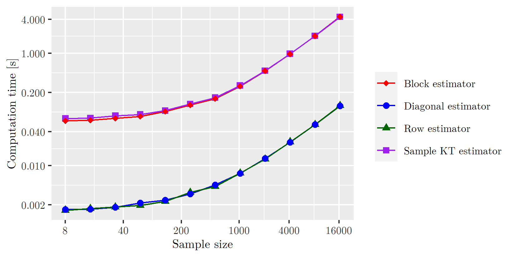
Figure 3: Log-log plot of the estimators’ mean computation time [s] as a function of the sample size, calculated using a block size of $40$.

4.1.2 Effect of the block size

We first study the behavior of the MSE with respect to varying block sizes with off-diagonal block Kendall’s taus of $0.1$ and diagonal block Kendall’s taus of $0.3$. In this experiment, we set the sample size to $4$ to reduce the computational cost of running a sufficient number of replications. Again, we examine data generated from the Gaussian and the Student’s t distributions. The MSEs and their 95% pointwise confidence intervals are calculated using 4000 replications. See Figure 4 for a log-log plot of the MSEs as a function block size.

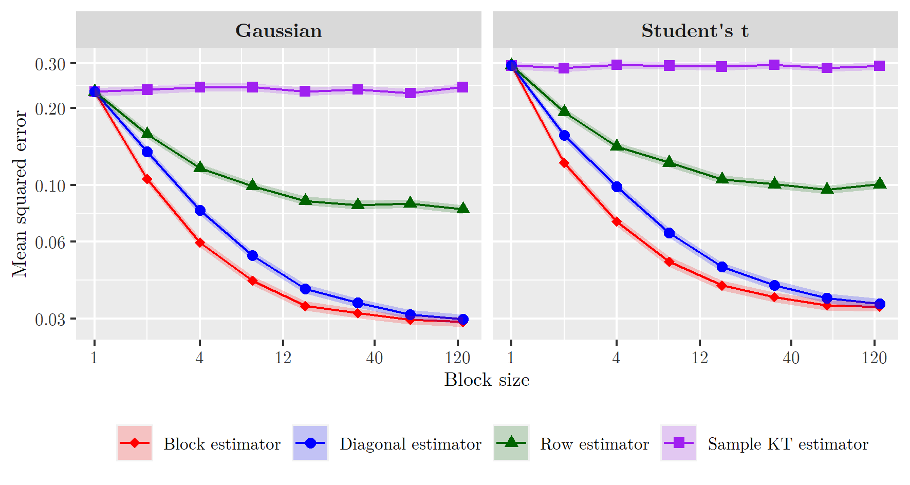
Figure 4: Log-log plots of the mean squared error as a function of the block size including 95% confidence intervals, calculated using a sample size of $4$. The diagonal block Kendall’s taus are set at $0.3$ and the off-diagonal block values at $0.1$.

Figure 4 shows that all of the averaging estimators perform increasingly better than the sample Kendall’s tau estimator for growing block dimensions. For large block dimensions the MSEs seem to reach constant values, confirming that the asymptotic variances do not depend on block dimensions. As expected, the block and diagonal averaging estimators both converge to the lowest limiting variance, approached fastest by the block averaging estimator. The row averaging estimator performs considerably less. The only difference we observe between the Gaussian and the Student’s t distribution is again that that the MSEs of the latter are slightly higher. This is not surprising as all of the variances depend on the underlying copula.

Figure 5: Log-log plots of the ratio $\text{MSE}(\widehat{\tau})/\text{MSE}(\widehat{\tau}^{B})$ as a function of the block size including 95% confidence intervals, calculated using a sample size of $4$. The diagonal block Kendall’s taus are set at $0.3$ and the off-diagonal block values at $0.1$.

To better visualize the difference in order of magnitude between the MSEs of the estimators $\widehat{\tau}$, we plot the ratio $\text{MSE}(\widehat{\tau})/\text{MSE}(\widehat{\tau}^{B})$ as a function of the block size, where $\widehat{\tau}$ denotes any of the row, diagonal and naive estimators. The results are depicted in Figure 5 including 95% confidence intervals. On this figure, we see that for both the Gaussian and Student’s t distributions the averaging estimators seem to improve on the sample Kendall’s tau estimator by roughly the same order of magnitude. Note, however, that these improvements do theoretically depend on the underlying copula. This result thus indicates that the exact form of the copula makes little difference to the improvement on the sample Kendall’s tau matrix estimator when the copula resembles to some extent the Gaussian or Student’s t copulas. Furthermore, we find that the relative difference between the diagonal and block estimator is largest for small dimensions, but they are still well within a factor of $1.5$ of each other. As the dimension increase, the MSEs of the diagonal estimator converge rapidly to that of the block estimator, again confirming that the block and diagonal estimators have close variances for large block dimensions.

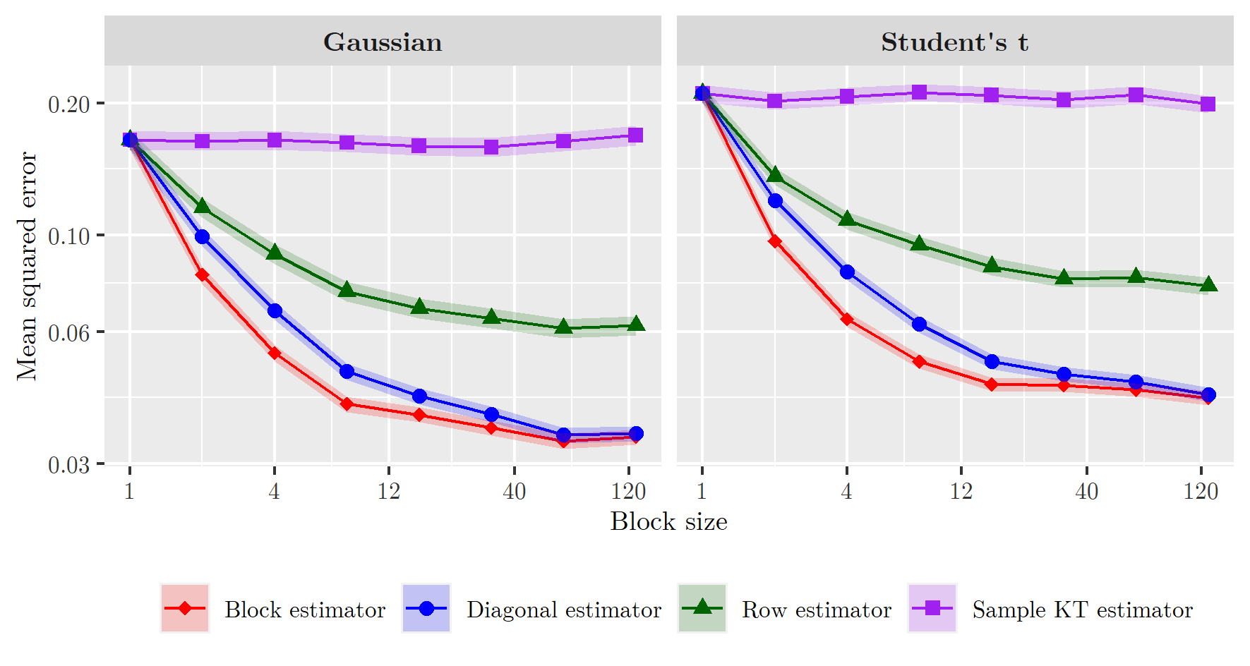
Figure 6: Log-log plots of the unconditional estimators’ mean squared error as a function of the block size including 95% confidence intervals, estimated using a sample size of $4$. The diagonal block target Kendall’s taus are set at $0.5$ and the off-diagonal block values at $-0.5$.

Figure 7: Log-log plots of the ratio $\text{MSE}(\widehat{\tau})/\text{MSE}(\widehat{\tau}^{B})$ as a function of the block size including 95% confidence intervals in the unconditional framework. The diagonal block Kendall’s taus are set at $0.5$ and the off-diagonal block values at $-0.5$.

Next, let us investigate the estimators’ MSEs under the less realistic target values of $-0.5$ in the off-diagonal block and $0.5$ in the diagonal blocks. Similarly, we set the sample size to $4$ since this does not affect the relative performance of the estimators, and examine data generated from both the Gaussian and Student’s t distributions. The MSEs and 95% confidence intervals are estimated using 4000 replications. See Figure 6 for a plot of the MSEs as a function of the block size and see Figure 7 for the corresponding ratio plot.

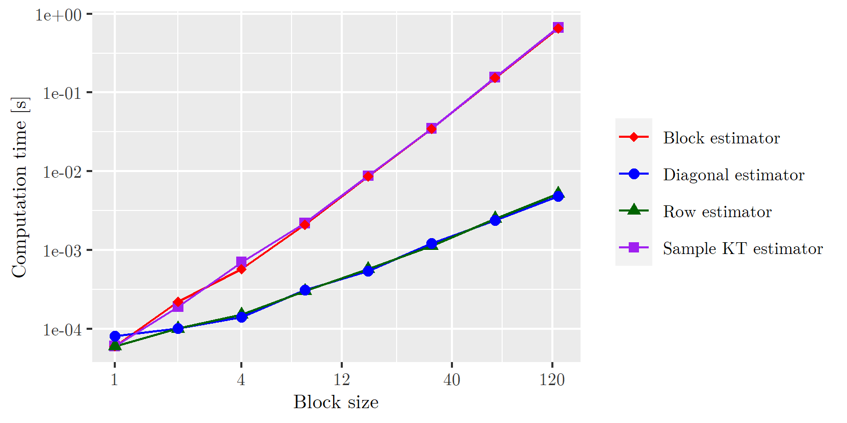
Figure 8: Log-log plot of the unconditional estimators’ mean computation time [s] as a function of the block size.

On Figure 6, we observe analogous results to the more realistic target values: all estimators are improvements over the naive estimator, the block and diagonal estimators have the best limiting variance, with the block estimator having the fastest convergence. Also, the MSEs generated from the student’s t distribution are slightly higher than for the Gaussian distribution, but the order of magnitudes with which the averaging estimators improve are comparable again. It is however noticeable that these order of magnitudes are considerably lower when compared to the setting with the more realistic target Kendall’s tau values, i.e. roughly 4 versus 8 for the block and diagonal estimators. This comes as no surprise; the diagonal block Kendall’s tau are higher, reducing the degree of independence of the pairwise estimates of the off-diagonal block’s, and thus reducing the effect of averaging.

For comparison of the computation efficiency, we perform 1000 replications with the same parameters as before. In Figure 8 the averages of the computation times can be found on log-log scale. As expected, we observe that both the sample Kendall’s tau matrix estimator and the block estimator scale quadratically with block size and that the row and diagonal estimators both scale linearly with block size. Consequently, for larger block dimensions one may prefer the diagonal estimator over the block estimator to gain substantial computational efficiency and lose only little precision.

4.2 Conditional Kendall’s Tau

In this section, we study the conditional versions of the block and diagonal estimators. Since the estimators make use of kernel regression, a larger sample size is needed for obtaining stable results. We therefore consider only a one-dimensional covariate $Z$, so that we do not need to increase the sample size even further and can run a sufficient number of replications. Kernel estimation is carried out with the Epanechnikov kernel and the estimation procedures are now available in the function CKTmatrix.kernel of the R package CondCopulas [5].

In each of the experiments, we let the covariate $Z$ be uniformly distributed on the interval $[0,1]$. We will estimate conditional Kendall’s taus for points $z$ ranging from 0 to 1 in steps of 0.1. We generate data with the Gaussian distribution, as the Student’s t distribution yields similar results. All variables will have a mean of $Z$ and variance of $1+Z^{2}$. The Kendall’s tau matrix is again block-structured corresponding to two groups of equal size. Similarly to the unconditional case, we only focus on the estimates of the single off-diagonal block. We set all Kendall’s taus within the diagonal blocks to a constant value of $0.3$, which is independent of $Z$. Finally, we let the Kendall’s taus within the off-diagonal block depend on the covariate $Z$.

In Section 4.2.1 and Section 4.2.2, we examine the accuracy and computational efficiency of the estimates under varying sample size and block dimensions. To this end, we set Kendall’s tau in the off-diagonal blocks to $0.1\,Z$. As $Z$ is distributed on $[0,1]$, the conditional Kendall’s taus range from $0$ to $0.1$. As such, the underlying variables are again partially exchangeable conditionally to $Z=z$ for any $z\in[0,1]$. It follows that the biases of the pairwise estimates in the off-diagonal block are all equal and thus that averaging over them does not change the total bias. Since therefore all estimators have equal biases, we focus on the sample variances instead of the MSEs for a comparison of accuracies.

Then, in Section 4.2.3 we study optimal bandwidths where we vary the way in which the off-diagonal block Kendall’s taus depend on $Z$. We consider a model in which we let the off-diagonal block conditional Kendall’s taus be given by

$$\left[{\mathbf{T}}_{|Z=z}\right]_{\mathcal{B}_{1,2}}=0.1(\cos(0.5\pi\omega z)+1){\bf 1},$$

with frequencies $\omega$ in $\{1,2,3,4\}$. As such, these conditional Kendall’s taus range from $0$ until $0.2$. For comparing the accuracies under varying bandwidths, we study mean integrated squared errors (MISE) computed by averaging the MSEs of conditional estimates computed at conditioning points ranging from $0$ to 1 in steps of 0.1.

4.2.1 Effect of the sample size

In this experiment, we study the dependency of the variances on the sample size. To this end, we vary the sample size under a fixed block size of $4$ and a bandwidth of $0.5$. We use this relatively large bandwidth to ensure stable results even at lower sample sizes. The sample variances and 95% confidence intervals are estimated using 8000 replications. For each grid point $z$ we plot the resulting sample variances on log-log scale in Figure 11.

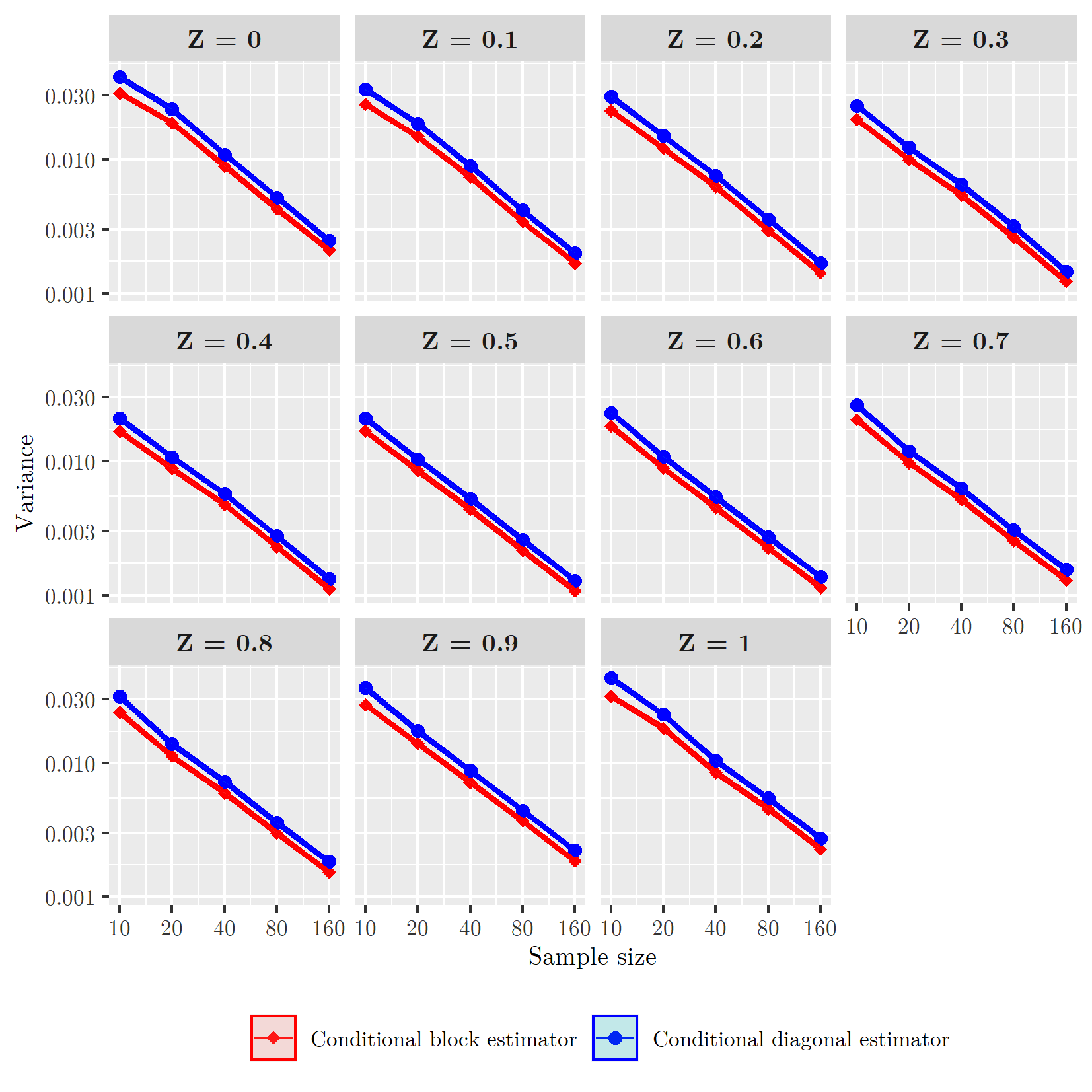
Figure 9: Log-log plots of the conditional estimators’ variances as a function of the sample size on several conditioning points including 95% confidence intervals, using a block size of $4$ and a bandwidth of 0.5.

Unsurprisingly, the conditional variances are also inversely related to the sample size. It follows that if bandwidths are kept constant, MSEs converge to the bias. As such, appropriate bandwidths are naturally smaller for larger sample sizes. Furthermore, it is seen that the estimates near the edges of the interval $[0,1]$ are less accurate than those in the middle. This can be attributed to the fact that there are fewer observations of $Z$ near grid points close to the edges than near grid points in the middle, since the observations can be found there on both sides. Evidently, a change in the distribution of $Z$ also changes the level of the variances.

Next, let us study the dependency of the computation time on the sample size. We leave the setting unchanged, though the results correspond to the calculation of the conditional block estimates on a single grid point. The results are computed using 500 replications and are represented on log-log scale in Figure 10. Here it is seen that the computation times gradually increase with the sample sample to a point where they appear to scale quadratically with each other. This behavior follows from the fact that the conditional estimates require the calculation of a double sum of $n$ terms. Note that the computation times of the diagonal and block estimators are relatively close since only a block size of $4$ is used here.

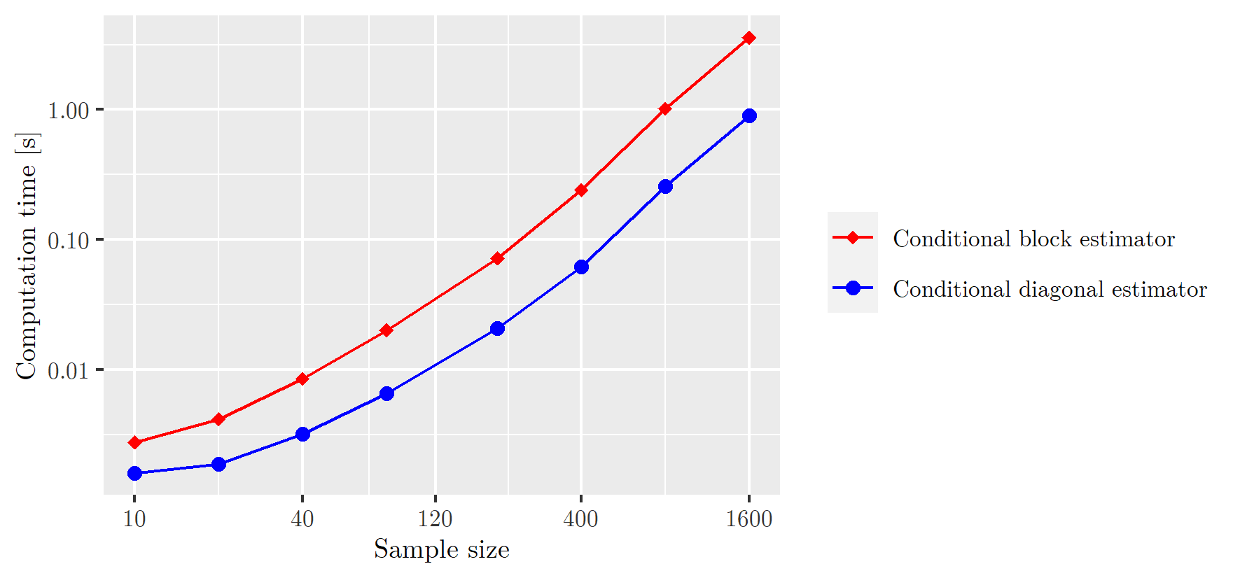
Figure 10: Log-log plot of the mean computation time [s] of the conditional estimator as a function of the sample size, for a block size of 4.

4.2.2 Effect of the block size

We first study the estimators’ variance under varying block dimensions. In order to run a sufficient number of replications we set the sample size to 20 and consequently the bandwidth to 0.5. The variances and 95% confidence intervals are estimated using 30000 replications. For each grid point $z$, the resulting sample variances are displayed on log-log scale in Figure 11.

From the figure we observe that the estimators’ variances behave similarly to the unconditional setting under varying block dimensions, for each of the grid points. That is, both estimators are improvements over the naive estimator, both limiting variances are identical, and the block estimator converges slightly faster than the diagonal estimator. It further follows that since averaging reduces variance, it also reduces the optimal bandwidth. This will be studied in more detail in Section 4.2.3. Again, as there are fewer observations of $Z$ near grid points close to the edges of $[0,1]$, the variance levels vary slightly over the different grid points.

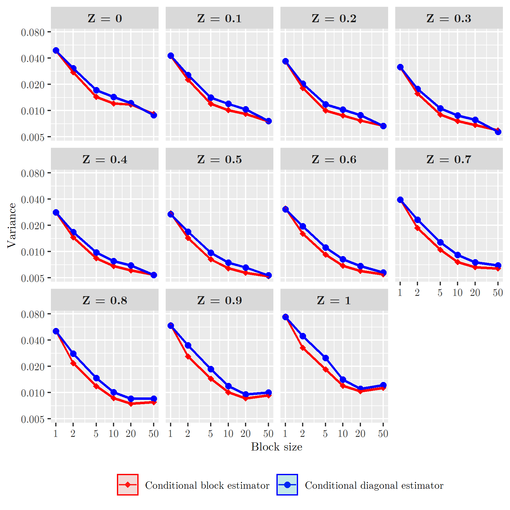
Figure 11: Log-log plots of the conditional estimators’ variances as a function of the sample size on several conditioning points including 95% confidence intervals, for a sample size of $20$ and a bandwidth of 0.5.

As for the computation times, there is clearly no fundamental change in how these depend on the block size when compared to the unconditional setting. However, since the conditional estimators are kernel-based, it should be noted that they generally require more computation time than their unconditional counterparts, as was also seen in Figure 10. For the sake of completeness, we still include a plot of the average computation time against the block size, see Figure 12. The results correspond to estimating the off-diagonal block conditional Kendall’s taus simultaneously on the $11$ grid points, and follow from $10000$ replications with a sample size of $150$. As expected, the block estimator scales quadratically with block size, while the diagonal estimator scales linearly with block size. Therefore, as in the unconditional case, one may prefer the diagonal estimator over the block estimator to gain substantial computational efficiency and lose only little precision.

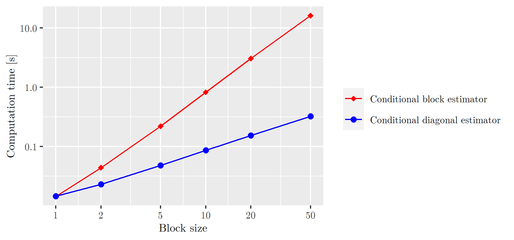
Figure 12: Log-log plot of the conditional estimators’ mean computation time [s] as a function of the block size, for a sample size of $150$.

4.2.3 Bandwidth selection

Let us compare the estimators’ MISEs for different bandwidths. In this experiment, we set the diagonal block Kendall’s taus to 0.3 and the off-diagonal block Kendall’s taus conditionally at $Z=z$ to

$$0.1(\cos(0.5\pi\omega z)+1),$$

with frequencies $\omega\in\{1,2,3,4\}$. The block size is fixed at $8$ and the sample size at $200$. The MISEs and 95% confidence intervals are estimated using 100 replications, see Figure 13.

The figure confirms that indeed the averaging estimators have smaller optimal bandwidths than the naive estimator. It should be noted that only a block size of $8$ is used here, and that the optimal bandwidth decreases with block size until the limit values are reached. Furthermore, the figure shows that as the frequency increases, the optimal bandwidth is reduced. This is fully consistent with kernel regression theory: increasing the frequency increases the difference in Kendall’s tau values conditionally on adjacent points of $z$, and therefore we need to pick a smaller bandwidth. Lastly, it should be noted that as the bandwidth increases the effect of averaging is less and less visible. This can be attributed to the fact that by increasing the bandwidth, the variance term within the MISE becomes less and less prominent, while the bias term generally increases.

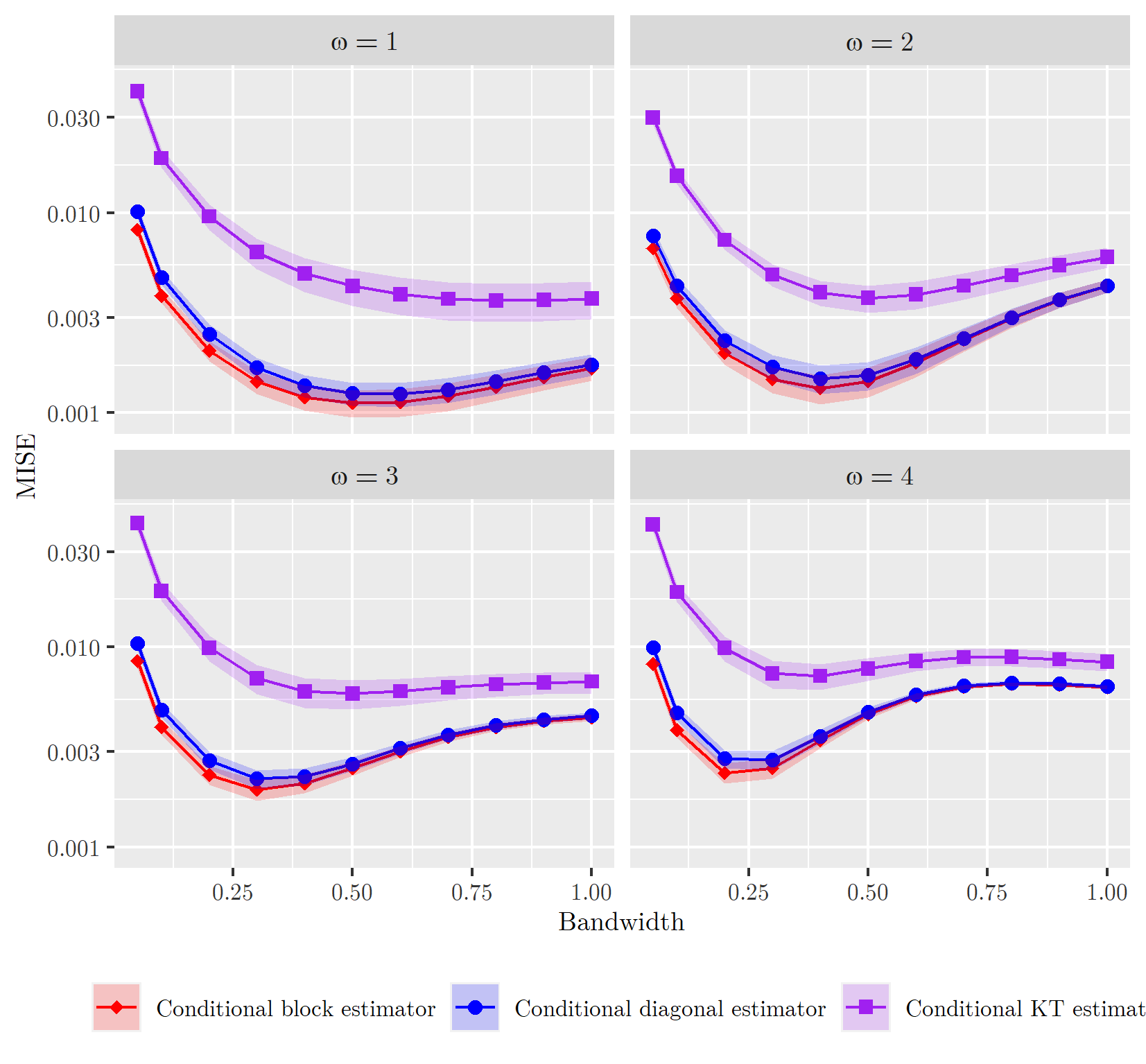
Figure 13: Log-plots of the conditional estimators’ MISEs as a function of the bandwidth for different frequencies $\omega$ including 95% confidence intervals, for a sample size of 200 and a block size of 8.

5 Application to Real Data

In this section, we study the behavior of the estimators under real data conditions and provide value at risk (VaR) computations of a large stock portfolio as an example of possible applications. In Section 5.2, we describe the methods used to estimate the VaR input parameters. The results are presented in Section 5.3, where backtesting is applied to asses the viability. All computations have been done using the R statistical environment [31].

5.1 VaR for Elliptical Distributions

The value at risk is a widely used risk measure in a variety of financial fields, ranging from auditing and financial reporting to risk management and the calculation of regulatory capital [25]. It is used to quantify potential losses over a specific time frame of some financial entity or portfolio of assets. We will follow the approach of [30, 33], in which explicit expressions for the value at risk of elliptical distributions was derived. For the reader’s convenience, we recall these expressions in the present section.

Let $X$ be a loss function (with negative losses and positive profits), then we define the VaR at level $\alpha\in(0,1)$ as the smallest number $x$ such that the probability that $X$ does not exceed $x$ is at least $1-\alpha$. More formally,

$$\operatorname{VaR}_{\alpha}(X):=-\inf\left\{x\in\mathbb{R}:F_{X}(x)>\alpha\right\},$$

or equivalently by setting $Y:=-X$,

$$\operatorname{VaR}_{\alpha}(X)=F_{Y}^{-1}(1-\alpha).$$ (13)

To calculate the VaR of a given portfolio of assets, it is often assumed that the portfolio’s profits and losses are a linear function of the returns of the individual constituents. More formally, a portfolio with value $\Pi(t)$ at time $t$ is called linear if its profit and loss $\Delta\Pi(t)=\Pi(t)-\Pi(0)$ over a time window $[0,\mathrm{t}]$ is a linear function of the returns $X_{1}(t),\ldots,X_{p}(t)$:

$$\Delta\Pi(t)=\delta_{1}X_{1}(t)+\delta_{2}X_{2}(t)+\ldots+\delta_{p}X_{p}(t).$$

This clearly applies to any common stock portfolio by using the ordinary returns of the individual shares and when considering the log returns, this holds to a good approximation provided that the time window $[0,t]$ is small, e.g. for daily log returns. The time window $t$ will be kept constant and will therefore be omitted from future notations.

Furthermore, we will assume that the $X_{j}$ are elliptically distributed with mean $\boldsymbol{\mu}$, covariance matrix $\boldsymbol{\Sigma}$ with Cholesky decomposition $\boldsymbol{\Sigma}=\mathbf{A}\mathbf{A}^{T}$ and density generator $g$. Thus, the probability density function $f_{\mathbf{X}}$ of $\mathbf{X}=(X_{1},\ldots,X_{p})$ is given by

$$f_{\mathbf{X}}(\mathbf{x})=\lvert\boldsymbol{\Sigma}\rvert^{-1/2}g\left((\mathbf{x}-\boldsymbol{\mu})^{T}\boldsymbol{\Sigma}^{-1}(\mathbf{x}-\boldsymbol{\mu})\right).$$

When considering elliptically distributed risk factors, we cannot simply use the Delta-Normal approach to calculate the VaR, as it relies on the stronger assumption of normality. A generalization of the Delta-Normal method was derived for the class of elliptical distributions in [33].

Let us start by noting that the VaR of the portfolio profits and losses $\Delta\Pi(t)$ as given in (13) can be rewritten as $\mathbb{P}\left(\Delta\Pi<-\operatorname{VaR}_{\alpha}\right)=\alpha.$ Then, given the linearity of the portfolio and the fact that $\mathbf{X}$ follows an elliptical distribution, the VaR is obtained by solving the following equation:

$$\alpha=|\boldsymbol{\Sigma}|^{-1/2}\int_{\left\{\boldsymbol{\delta}\mathbf{x}^{T}\leq-\operatorname{VaR}_{\alpha}\right\}}g\left((\mathbf{x}-\boldsymbol{\mu})\boldsymbol{\Sigma}^{-1}(\mathbf{x}-\boldsymbol{\mu})^{T}\right)\mathrm{d}\mathbf{x},$$

where $\boldsymbol{\delta}$ denotes the vector of weights $(\delta_{1},\ldots,\delta_{p})$. After several changes of variables, we obtain

$$\alpha=\left|S_{p-2}\right|\int_{0}^{\infty}r^{p-2}\int_{-\infty}^{\frac{-\boldsymbol{\delta}\boldsymbol{\mu}^{T}-\operatorname{VaR}_{\alpha}}{|\boldsymbol{\delta}\mathbf{A}|}}g\left(z_{1}^{2}+r^{2}\right)\mathrm{d}z_{1}\mathrm{d}r,$$ (14)

where $\left|S_{p-2}\right|:=2\pi^{\frac{p-1}{2}}/\Gamma(\frac{p-1}{2}).$ Let us now introduce the function

$$G(s) =\frac{2\pi^{\frac{p-1}{2}}}{\Gamma(\frac{p-1}{2})}\int_{-\infty}^{-s}\int_{0}^{\infty}r^{n-2}g(z_{1}^{2}+r^{2})\mathrm{d}r\mathrm{d}z_{1}=\frac{\pi^{\frac{p-1}{2}}}{\Gamma(\frac{p-1}{2})}\int_{s}^{\infty}\int_{z}^{\infty}(u-z^{2})^{\frac{p-3}{2}}g(u)\mathrm{d}u\mathrm{d}z,$$ (15)

where we have changed variables to $u=r^{2}+z_{1}^{2}$ and $z=-z_{1}$. Let us denote by $q_{\alpha,p}^{g}$ the unique solution of the transcendental equation

$$\alpha=G(q_{\alpha,p}^{g}).$$ (16)

It then finally follows from expressions (14) and (15) that the Delta-Elliptic VaR is given by

$$\operatorname{VaR}_{\alpha} =-\boldsymbol{\delta}\boldsymbol{\mu}^{T}+q_{\alpha,p}^{g}|\boldsymbol{\delta}\mathbf{A}|=-\boldsymbol{\delta}\boldsymbol{\mu}^{T}+q_{\alpha,p}^{g}\sqrt{\boldsymbol{\delta}\boldsymbol{\Sigma}\boldsymbol{\delta}^{T}}.$$ (17)

Note that this equation has a clear financial interpretation: the portfolio’s average return is given by $\boldsymbol{\delta}\boldsymbol{\mu}^{T}$ and the portfolio’s standard deviation by $\sqrt{\boldsymbol{\delta}\boldsymbol{\Sigma}\boldsymbol{\delta}^{T}}$. Further note that the result is analogous to that of the Delta-Normal VaR, in which we simply replace $q_{\alpha,p}^{g}$ with the $1-\alpha$ quantile of the standard-normal distribution.

5.2 Estimation Procedure

In order to test the estimators in real data conditions, we consider a portfolio consisting of $240$ different stocks. All stocks are listed on the Euronext markets and data has been downloaded from Yahoo Finance. The complete list of all shares involved is available in Appendix B. We will estimate the portfolio’s daily VaR assuming that the price is set at a level of 100 and that all stocks in the portfolio are equally weighted. To this end, we model the daily log returns of the individual stocks, assuming they follow an elliptical distribution.

In order to achieve a proper clustering, we compute the pairwise Kendall’s tau matrix over a long time period from 01 January 2007 to 14 January 2022, after which we reorder the variables in order to obtain the intended block structure. Since we have not proposed a clustering method, we simply use the method GW_Ward method from package seriation [18], along with a few manual adjustments. The resulting reordering corresponds to four large groups, which are specified further in Appendix B. See Figure 1 for a heatmap of the pairwise Kendall’s tau matrix before and after reordering the variables by group. To indicate the groups, lines have been drawn around the diagonal blocks. It should be noted that, if studied carefully, the large groups can be broken down into smaller and more accurate groups. Nevertheless, these large groups already seem to be quite useful and therefore we will simply use them for our further analysis.

Based on the groups displayed in Figure 1, the objective is to compute the VaR at 30 June 2017, leaving sufficient future data for backtesting the results. To this end, we estimate the Kendall’s tau matrix of the log returns using the block, row, diagonal and sample Kendall’s tau matrix estimators using data points over the period 01 August 2015 to 30 June 2017. To estimate the standard deviations and averages over the same period, we use the sample mean and sample standard deviation.

Following the elliptical assumption, we can now obtain covariance matrix estimates from each of the Kendall’s tau matrix estimates. Subsequently, we can compute nonparametric estimates of the density generator for each of these inputs. To this end, we make use of the function EllDistrEst from the ElliptCopulas package [9] which implements Liebscher’s procedure [21].

For the density generator estimation we require a complete data set with no missing values. As such, the interval on which we estimate the density generator will be chosen as shorter (01 June 2016 to 30 June 2017). The kernel function will be chosen as the Epanechnikov kernel. Further we use Silverman’s rule of thumb for bandwidth selection to estimate elliptical density generators [30], which for a sample size of $n$ is given by

$$h=1.06\sqrt{\operatorname{Var}\left[\widehat{\boldsymbol{\xi}}\right]n^{1/5}},$$ (18)

where

$$\widehat{\xi}_{i}=-1+\left(1+((\mathbf{x}_{i}-\boldsymbol{\mu})\widehat{\boldsymbol{\Sigma}}^{-1}(\mathbf{x}_{i}-\boldsymbol{\mu}))^{p/2}\right)^{2/p},$$

for $i=1,\ldots,n$ and $p=240$. Here, $\mathbf{x}_{i}$ stands for the vector of log returns at the $i$th date, $\widehat{\boldsymbol{\Sigma}}$ stands for one of the covariance matrix estimates and $\boldsymbol{\mu}$ stands for the log returns’ sample mean. Clearly, by using this bandwidth selection method, the use of different Kendall’s tau matrix estimators yields different values for the bandwidth. In order to get a better idea of the effects of the bandwidth choice, we also consider several deterministic bandwidths, and compare the performance of the estimators for each of them.

Finally, we can numerically solve the transcendental equation as given in (14) to arrive at the corresponding quantiles. As such, we have discussed all ingredients for calculating the VaR as in (17). In order to test the results, we perform backtesting on two intervals, one in the future from 01 July 2017 to 14 January 2022 and one during the period on which the estimations are based, from 01 August 2015 to 30 June 2017.

5.3 Results

We compute the portfolio’s 5% and 10% VaR values by following the estimation procedure described in Section 5.2. Table 1 shows the quantile estimates obtained by solving the transcendental equation for each of the different density generator estimates. The density generators were estimated using each of the block, row, diagonal and naive Kendall’s tau matrix estimators and using varying values of the bandwidth.

The table shows that the averaging estimators yield very similar quantiles which are all relatively constant for different choices of the bandwidth. In contrast, the quantiles of the naive estimator lie substantially higher and vary significantly for the different bandwidths. In that sense, the estimates obtained with the averaging estimators seem to be much more stable. Moreover, the Silverman’s bandwidths of the averaging estimators are also all very similar, while that of the naive estimator is again considerably larger.

Table 1: Estimated quantiles corresponding to the 5% and 10% VaRs calculated by estimating an elliptical distribution for the daily log returns using each of the different Kendall’s tau matrix estimates and several values of the bandwidth.

Quantiles $\boldsymbol{q_{\alpha,p}^{\widehat{g}_{h}}}$		Estimated
$\alpha$	Estimator	$h=20$	$h=40$	$h=100$	Silverman’s $h$
5%	Naive	2.11	1.94	1.98	2.12 ($h=586.8$)
	Block	1.60	1.60	1.60	1.60 ($h=40.8$)
	Row	1.60	1.60	1.60	1.60 ($h=41.1$)
	Diagonal	1.59	1.59	1.60	1.59 ($h=40.5$)
10%	Naive	1.48	1.38	1.40	1.53 ($h=586.8$)
	Block	1.23	1.23	1.23	1.23 ($h=40.8$)
	Row	1.24	1.24	1.23	1.24 ($h=41.1$)
	Diagonal	1.23	1.23	1.23	1.23 ($h=40.5$)

Table 2 shows the VaR estimates for each of the different estimators and bandwidths, and also the backtested VaR values. As discussed in Section 5.2, backtests were conducted at two intervals, interval 1 refers to the upcoming interval from 01 July 2017 until 14 January 2022, and interval 2 refers to the interval on which the estimation is based, from 01 August 2015 until 30 June 2017.

Table 2: Estimated 5% and 10% VaRs including the corresponding backtesting results on two intervals. Interval 1 corresponds to 01 July 2017 until 14 January 2022 and interval 2 to 01 August 2015 until 30 June 2017.

$\boldsymbol{\operatorname{VaR}}$		Estimated				Backtested
$\alpha$	Estimator	$h=20$	$h=40$	$h=100$	Silverman’s $h$	Interval 1	Interval 2
5%	Naive	1.647	1.512	1.544	1.655 ($h=586.8$)	1.392	1.262
	Block	1.320	1.320	1.320	1.320 ($h=40.8$)
	Row	1.332	1.332	1.332	1.332 ($h=41.1$)
	Diagonal	1.284	1.284	1.292	1.284 ($h=40.5$)
10%	Naive	1.147	1.083	1.068	1.187 ($h=586.8$)	0.861	0.839
	Block	1.008	1.008	1.008	1.008 ($h=40.8$)
	Row	1.026	1.017	1.026	1.026 ($h=41.1$)
	Diagonal	0.987	0.987	0.987	0.987 ($h=40.5$)

Table 3: The number of exceedances of the estimated 5% and 10% VaRs during backtesting interval 1, from 01 July 2017 until 14 January 2022.

# Exceedances		Estimated				Backtested
$\alpha$	Estimator	$h=20$	$h=40$	$h=100$	Silverman’s $h$	Interval 1
5%	Naive	47	53	53	46 ($h=586.8$)	58
	Block	58	58	58	58 ($h=40.8$)
	Row	58	58	58	58 ($h=41.1$)
	Diagonal	61	61	59	61 ($h=40.5$)
10%	Naive	76	85	83	72 ($h=586.8$)	116
	Block	94	94	94	94 ($h=40.8$)
	Row	91	91	92	91 ($h=41.1$)
	Diagonal	100	100	100	100 ($h=40.5$)

Table 4: The number of exceedances of the estimated 5% and 10% VaRs during backtesting interval 2, from 01 August 2015 until 30 June 2017.

# Exceedances		Estimated				Backtested
$\alpha$	Estimator	$h=20$	$h=40$	$h=100$	Silverman’s $h$	Interval 2
5%	Naive	9	12	12	9 ($h=586.8$)	25
	Block	20	20	20	20 ($h=40.8$)
	Row	20	20	20	20 ($h=41.1$)
	Diagonal	22	22	21	22 ($h=40.5$)
10%	Naive	30	32	32	30 ($h=586.8$)	49
	Block	35	35	35	35 ($h=40.8$)
	Row	35	35	35	35 ($h=41.1$)
	Diagonal	35	35	35	35 ($h=40.5$)

This clearly shows that the averaging estimators have performed significantly better than the naive estimator when compared to both backtesting intervals. For both $\alpha$-levels, it can be seen that the VaRs generated using the naive estimator are considerably larger than those using the averaging estimators, which themselves produce relatively similar values. Furthermore, it can be seen that the 5% VaRs of the averaging estimators agree fairly well with the results of the backtesting, unlike those of the naive estimator.

However, the 10% VaR estimates are not as accurate and all estimators yield considerably higher VaRs than those obtained by backtesting. This could indicate that the log returns are not elliptically distributed, or that the interval at which we estimate the density generator is too short. Recall that the interval on which we estimate the density generator is merely from 01 June 2016 until 30 June 2017.

To get a better understanding of how well the VaR estimates correspond with the backtesting results, we examine how often the estimates are exceeded by the portfolio’s losses in each of the backtesting periods. Table 3 and 4 show the number of exceedances in interval 1 and interval 2 respectively.

Both tables show that the difference between the theoretical and the observed number of exceedances is much larger when using the naive sample Kendall’s tau matrix estimator than when using any of the averaging estimators and this applies to both $\alpha$-levels as well as to all bandwidths. As such, the averaging estimators are overall significantly better performers than the naive estimator. In addition, although there are subtle differences in the performance of the block, row and diagonal estimators, there is no clear winner in this example. This shows that computing all Kendall’s tau using the block estimators incur no clear additional benefits compared to using only the row or diagonal estimators, that are computationally much cheaper.

6 Conclusion

We have provided an alternative approach to the generally challenging task of estimating Kendall’s tau and conditional Kendall’s tau matrices in high-dimensional settings. By imposing structural assumptions on the underlying (conditional) Kendall’s tau matrix, we have introduced new estimators that have significantly reduced computational costs without much loss in performance.

For the unconditional case, a model was studied in which the set of variables could be grouped in such a way that the Kendall’s taus of variables from different groups depends only on the group numbers. After reordering the variables by group, the underlying Kendall’s tau matrix is then block-structured with constant values in the off-diagonal blocks. We have proposed several (unbiased) estimators that take advantage of this block-structure by averaging over the usual pairwise Kendall’s tau estimates in each of the off-diagonal blocks: the block estimator averages over all pairwise estimates, whereas the row, the diagonal and the random estimators only average over part of the off-diagonal blocks (respectively, over the pairs on the first row, on the first diagonal and over a random selection of pairs).

We have formally derived variance expressions, which showed not only that all estimators are improvements over the usual sample Kendall’s tau matrix estimator, but also, interestingly, that the asymptotic variances do not depend on the block dimensions. Furthermore, we have seen that the block, the diagonal and the random estimators have very similar asymptotic variances, whereas that of the row estimator was different. The former depend on the auxiliary quantity $U$, while the latter depends on $S$. In each example that has been studied, we saw that the $U$-asymptotic variances were lower than the $S$-asymptotic variances, but a formal characterization of the set of copulas to which this applies is left for future work. Under light assumptions, we have shown that $U$-asymptotic variances are equal, and that it is approached fastest by the block estimator, followed by the diagonal estimator and then the random estimator. Hence, if the computational costs were to be reduced, the diagonal estimator is preferable to both the random and the row estimator.

Furthermore, a model was studied in which the Kendall’s taus depend on a conditioning variable. Here it was assumed that the conditional Kendall’s tau matrix has the above-mentioned block structure and, moreover, that it is preserved under fluctuations of the conditioning variable. We have adopted nonparametric, kernel-based estimates of the conditional Kendall’s tau in order to construct the conditional versions of the block, row, diagonal and random estimators. Under some additional regularity assumptions, we have shown that the estimators are all asymptotically normal conditionally to different values of the covariate. Following from these expressions, we have seen that the asymptotic variances have analogous expressions to their unconditional counterparts. As such, all estimators are again improvements over the naive estimator, with the block estimator having the best performance. Similarly, if computational costs were to be reduced, the diagonal estimator is preferable to both the random and the row estimator. Moreover, the reduction of computing costs becomes particularly relevant in the conditional setting, as the use of kernel smoothing introduces additional complexity.

We have performed a simulation study in order to support the theoretical findings. In the unconditional setting, simulations were performed with the Gaussian and Student’s t distributions. It was furthermore confirmed that the diagonal and the block estimator indeed have the lowest asymptotic variance, with the block estimator converging the fastest, though closely followed by the diagonal estimator. This emphasizes the practical use of the diagonal estimator.

We remarked again that the conditional estimators’ variances decrease in a similar fashion for growing block dimensions. As a consequence, the averaging estimators allow for a reduced optimal bandwidth; this was indeed confirmed in the simulations. This makes the averaging estimators perfectly suited for practical applications, as reducing the bandwidth goes hand in hand with reducing the estimation bias.

Lastly, we have demonstrated the use of the estimators in a real world application. The estimators were used to model the daily log returns of a large stock portfolio consisting of 240 Euronext listed stocks. After clustering the sample Kendall’s tau matrix, the proposed block structure was clearly visible. Building on these groups, robust estimates of the correlation matrix were obtained by assuming that the log returns follow an elliptical distribution. Using each of these estimates, the portfolio’s 5% and 10% VaR values were estimated. The results of the averaging estimators were much more stable under changes in the bandwidth used for the estimation of the density generator. Moreover, the averaging VaRs were significant improvements over the naive estimates. This example confirmed that the proposed block structures are well reflected in real data conditions and that the averaging estimators lead to significantly more stable and accurate results.

Acknowledgments. The authors thanks Thomas Nagler for useful comments on a previous draft, and Dorota Kurowicka for a discussion and references that lead to Section 2.2.

Appendix A Proofs

A.1 Proofs for Section 2.2

Proof of Proposition 1.

Note that

$$M({\bf 1}_{1}-{\bf 1}_{2})=(1-\rho_{1},\rho_{1}-1,0,\dots,0)=(1-\rho_{1})({\bf 1}_{1}-{\bf 1}_{2})$$

$$M({\bf 1}_{b_{1}+1}-{\bf 1}_{b_{1}+2})=(0,\dots,0,1-\rho_{2},\rho_{2}-1,0,\dots,0)=(1-\rho_{2})({\bf 1}_{b_{1}+1}-{\bf 1}_{b_{1}+2})$$

This gives us a number of $(b_{1}-1)+(b_{2}-1)$ eigenvectors with eigenvalues $1-\rho_{1}$ and $1-\rho_{2}$ that are positive since $\rho_{1},\rho_{2}$ are smaller than $1$. Moreover, remark that

$$M{\bf 1}_{1:b_{1}}=(1+(b_{1}-1))\rho_{1}{\bf 1}_{1:b_{1}}+b_{1}\rho_{3}{\bf 1}_{b_{1}+(1:b_{2})}$$

$$M{\bf 1}_{b_{1}+(1:b_{2})}=b_{2}\rho_{3}{\bf 1}_{1:b_{1}}+(1+(b_{2}-1)\rho_{2}){\bf 1}_{b_{1}+(1:b_{2})},$$

so the eigenvalues of the matrix

$$\left(\begin{array}[]{cc}(1+(b_{1}-1)\rho_{1}&b_{1}\rho_{3}\\ b_{2}\rho_{3}&1+(b_{2}-1)\rho_{2}\end{array}\right)$$

are also eigenvalues of $M$. These eigenvalues are

$$1+\frac{\left(b_{1}-1\right)\rho_{1}}{2}+\frac{\left(b_{2}-1\right)\rho_{2}}{2}\pm\frac{\sqrt{\left(\left(b_{1}-1\right)\rho_{1}-\left(b_{2}-1\right)\rho_{2}\right)^{2}+4b_{1}\rho_{3}^{2}b_{2}}}{2}$$

The smallest eigenvalue is positive if and only if

$$\left(1+\frac{\left(b_{1}-1\right)\rho_{1}}{2}+\frac{\left(b_{2}-1\right)\rho_{2}}{2}\right)^{2}>\frac{\left(\left(b_{1}-1\right)\rho_{1}-\left(b_{2}-1\right)\rho_{2}\right)^{2}+4b_{1}\rho_{3}^{2}b_{2}}{4}.$$

i.e.

$$\Big{(}\big{(}b_{2}b_{1}-b_{1}-b_{2}+1\big{)}\rho_{2}+b_{1}-1\Big{)}\rho_{1}-b_{1}\rho_{3}^{2}b_{2}+(b_{2}-1)\rho_{2}+1>0$$

A sufficient condition is:

$$\rho_{1}>\frac{b_{1}b_{2}\rho_{3}^{2}-(b_{2}-1)\rho_{2}-1}{\left(b_{2}b_{1}-b_{1}-b_{2}+1\right)\rho_{2}+b_{1}-1},$$

$$\rho_{2}>-\frac{b_{1}-1}{b_{2}b_{1}-b_{1}-b_{2}+1}.$$

∎

Proof of Proposition 2.

Assume that $M$ is a correlation matrix, and let ${\mathbf{X}}\sim\mathcal{N}(0,M)$. Take one random variable from each block. Their correlation matrix is $(I+\rho J)$ and must therefore be positive semidefinite. This yields the constraint $\rho\geq-1/(K-1)$.

Conversely, this bound is reached by choosing the correlation matrices $\Sigma_{k}={\bf 1}$ for all $k=1,\dots,K$ and considering $M$ as the correlation matrix of $(X_{1},\dots,X_{1},X_{2},\dots,X_{2},\dots,X_{K},\dots,X_{K})\in{\mathbb{R}}^{b_{1}+b_{2}+\dots+b_{K}}$, where $(X_{1},\dots,X_{K})$ follows an exchangeable normal distribution with correlation arbitrarily close to $-1/(K-1)$. ∎

A.2 Derivation of Equation (4)

To derive the copula expression, we write

$$Q_{j_{1},j_{2}} =\mathbb{P}\big{(}(X_{j_{1}},X_{j_{2}})_{1}<(X_{j_{1}},X_{j_{2}})_{2},(X_{j_{1}},X_{j_{2}})_{1}<(X_{j_{1}},X_{j_{2}})_{3}\big{)}$$

$$+\mathbb{P}\big{(}(X_{j_{1}},X_{j_{2}})_{1}<(X_{j_{1}},X_{j_{2}})_{2},(X_{j_{1}},X_{j_{2}})_{1}>(X_{j_{1}},X_{j_{2}})_{3}\big{)}$$

$$+\mathbb{P}\big{(}(X_{j_{1}},X_{j_{2}})_{1}>(X_{j_{1}},X_{j_{2}})_{2},(X_{j_{1}},X_{j_{2}})_{1}>(X_{j_{1}},X_{j_{2}})_{3}\big{)}$$

$$+\mathbb{P}\big{(}(X_{j_{1}},X_{j_{2}})_{1}>(X_{j_{1}},X_{j_{2}})_{2},(X_{j_{1}},X_{j_{2}})_{1}<(X_{j_{1}},X_{j_{2}})_{3}\big{)}$$

where $(X_{j_{1}},X_{j_{2}})_{i}$ denotes the pair $(X_{j_{1},i},X_{j_{2},i})$. Let us write these probabilities in terms of the copula $C_{j_{1},j_{2}}$ of $(X_{j_{1}},X_{j_{2}})$. This gives

$$Q_{j_{1},j_{2}} =\int_{[0,1]^{2}}\int_{(u_{1},u_{2})}^{(1,1)}\int_{(u_{1},u_{2})}^{(1,1)}\mathrm{d}C_{j_{1},j_{2}}(u_{5},u_{6})\mathrm{d}C_{j_{1},j_{2}}(u_{3},u_{4})\mathrm{d}C_{j_{1},j_{2}}(u_{1},u_{2})$$

$$+\int_{[0,1]^{2}}\int_{(0,0)}^{(u_{1},u_{2})}\int_{(u_{1},u_{2})}^{(1,1)}\mathrm{d}C_{j_{1},j_{2}}(u_{5},u_{6})\mathrm{d}C_{j_{1},j_{2}}(u_{3},u_{4})\mathrm{d}C_{j_{1},j_{2}}(u_{1},u_{2})$$

$$+\int_{[0,1]^{2}}\int_{(u_{1},u_{2})}^{(1,1)}\int_{(0,0)}^{(u_{1},u_{2})}\mathrm{d}C_{j_{1},j_{2}}(u_{5},u_{6})\mathrm{d}C_{j_{1},j_{2}}(u_{3},u_{4})\mathrm{d}C_{j_{1},j_{2}}(u_{1},u_{2})$$

$$+\int_{[0,1]^{2}}\int_{(0,0)}^{(u_{1},u_{2})}\int_{(0,0)}^{(u_{1},u_{2})}\mathrm{d}C_{j_{1},j_{2}}(u_{5},u_{6})\mathrm{d}C_{j_{1},j_{2}}(u_{3},u_{4})\mathrm{d}C_{j_{1},j_{2}}(u_{1},u_{2})$$

$$=\int_{[0,1]^{2}}\bar{C}_{j_{1},j_{2}}^{2}(u_{1},u_{2})\mathrm{d}C_{j_{1},j_{2}}(u_{1},u_{2})+\int_{[0,1]^{2}}\bar{C}_{j_{1},j_{2}}(u_{1},u_{2})C_{j_{1},j_{2}}(u_{1},u_{2})\mathrm{d}C_{j_{1},j_{2}}(u_{1},u_{2})$$

$$+\int_{[0,1]^{2}}C_{j_{1},j_{2}}(u_{1},u_{2})\bar{C}_{j_{1},j_{2}}(u_{1},u_{2})\mathrm{d}C_{j_{1},j_{2}}(u_{1},u_{2})+\int_{[0,1]^{2}}C_{j_{1},j_{2}}^{2}(u_{1},u_{2})\mathrm{d}C_{j_{1},j_{2}}(u_{1},u_{2})$$

$$=\int_{[0,1]^{2}}(C_{j_{1},j_{2}}(u_{1},u_{2})+\bar{C}_{j_{1},j_{2}}(u_{1},u_{2}))^{2}\mathrm{d}C_{j_{1},j_{2}}(u_{1},u_{2}),$$

A.3 Proof of Lemma 3

Proof.

First check that, trivially, the sample Kendall’s tau $\widehat{\tau}_{j_{1},j_{2}}$ is a U-statistic of order 2 with (symmetric) kernel

$$g^{*}\left((X_{j_{1}},X_{j_{2}})_{i_{1}},(X_{j_{1}},X_{j_{2}})_{i_{2}}\right):=\operatorname{sign}\left(\left(X_{i_{1},j_{1}}-X_{i_{2},j_{1}}\right)\left(X_{i_{1},j_{2}}-X_{i_{2},j_{2}}\right)\right).$$

Consequently,

$$\widehat{\tau}_{k_{1},k_{2}}^{B} =\frac{1}{\lvert\mathcal{B}_{k_{1},k_{2}}\rvert}\sum_{(j_{1},j_{2})\in\mathcal{B}_{k_{1},k_{2}}}\widehat{\tau}_{j_{1},j_{2}}$$

$$=\frac{1}{\lvert\mathcal{B}_{k_{1},k_{2}}\rvert}\sum_{(j_{1},j_{2})\in\mathcal{B}_{k_{1},k_{2}}}\frac{2}{n(n-1)}\sum_{i_{1}<i_{2}}g^{*}\left((X_{j_{1}},X_{j_{2}})_{i_{1}},(X_{j_{1}},X_{j_{2}})_{i_{2}}\right)$$

$$=\frac{2}{n(n-1)}\sum_{i_{1}<i_{2}}\frac{1}{\lvert\mathcal{B}_{k_{1},k_{2}}\rvert}\sum_{(j_{1},j_{2})\in\mathcal{B}_{k_{1},k_{2}}}g^{*}\left((X_{j_{1}},X_{j_{2}})_{i_{1}},(X_{j_{1}},X_{j_{2}})_{i_{2}}\right),$$

and it follows that $\widehat{\tau}_{k_{1},k_{2}}^{B}$ is a U-statistic with kernel

$$g_{k_{1},k_{2}}^{B}\left(\mathbf{X}_{i_{1}},\mathbf{X}_{i_{2}}\right)=\frac{1}{\lvert\mathcal{B}_{k_{1},k_{2}}\rvert}\sum_{(j_{1},j_{2})\in\mathcal{B}_{k_{1},k_{2}}}g^{*}\left((X_{j_{1}},X_{j_{2}})_{i_{1}},(X_{j_{1}},X_{j_{2}})_{i_{2}}\right).$$

In a similar manner, it is easily seen that $\widehat{\tau}^{R}_{k_{1},k_{2}}$, $\widehat{\tau}^{D}_{k_{1},k_{2}}$ and $\widehat{\tau}^{U}_{k_{1},k_{2}}$ are all U-statistics as well with respective kernels

$$g_{k_{1},k_{2}}^{R}\left(\mathbf{X}_{i_{1}},\mathbf{X}_{i_{2}}\right) =\frac{1}{N_{k_{1},k_{2}}}\sum_{(j_{1},j_{2})\in(\mathcal{B}_{k_{1},k_{2}})_{R}}g^{*}\left((X_{j_{1}},X_{j_{2}})_{i_{1}},(X_{j_{1}},X_{j_{2}})_{i_{2}}\right),$$

$$g_{k_{1},k_{2}}^{D}\left(\mathbf{X}_{i_{1}},\mathbf{X}_{i_{2}}\right) =\frac{1}{N_{k_{1},k_{2}}}\sum_{(j_{1},j_{2})\in(\mathcal{B}_{k_{1},k_{2}})_{D}}g^{*}\left((X_{j_{1}},X_{j_{2}})_{i_{1}},(X_{j_{1}},X_{j_{2}})_{i_{2}}\right),$$

$$g_{k_{1},k_{2}}^{U}\left(\mathbf{X}_{i_{1}},\mathbf{X}_{i_{2}}\right) =\frac{1}{N_{k_{1},k_{2}}}\sum_{(j_{1},j_{2})\in\mathcal{B}_{k_{1},k_{2}}}W_{j_{1},j_{2}}g^{*}\left((X_{j_{1}},X_{j_{2}})_{i_{1}},(X_{j_{1}},X_{j_{2}})_{i_{2}}\right).$$

Note that the kernel $g_{k_{1},k_{2}}^{U}$ is random by depending on the weights $\mathbf{W}$. ∎

A.4 Proof of Theorem 4

Proof.

Recall from Lemma 3 that $\widehat{\tau}_{j_{1},j_{2}},\widehat{\tau}^{B}_{k_{1},k_{2}},\widehat{\tau}^{R}_{k_{1},k_{2}},\widehat{\tau}^{D}_{k_{1},k_{2}},\widehat{\tau}^{U}_{k_{1},k_{2}}$ can all be written as U-statistics of order 2 with the following symmetric kernels respectively

$$g^{*}\left((X_{j_{1}},X_{j_{2}})_{i_{1}},(X_{j_{1}},X_{j_{2}})_{i_{2}}\right) =\operatorname{sign}\left(\left(X_{i_{1},j_{1}}-X_{i_{2},j_{1}}\right)\left(X_{i_{1},j_{2}}-X_{i_{2},j_{2}}\right)\right)$$

$$g_{k_{1},k_{2}}^{R}\left(\mathbf{X}_{i_{1}},\mathbf{X}_{i_{2}}\right) =\frac{1}{N_{k_{1},k_{2}}}\sum_{(j_{1},j_{2})\in(\mathcal{B}_{k_{1},k_{2}})_{R}}g^{*}\left((X_{j_{1}},X_{j_{2}})_{i_{1}},(X_{j_{1}},X_{j_{2}})_{i_{2}}\right),$$

$$g_{k_{1},k_{2}}^{D}\left(\mathbf{X}_{i_{1}},\mathbf{X}_{i_{2}}\right) =\frac{1}{N_{k_{1},k_{2}}}\sum_{(j_{1},j_{2})\in(\mathcal{B}_{k_{1},k_{2}})_{D}}g^{*}\left((X_{j_{1}},X_{j_{2}})_{i_{1}},(X_{j_{1}},X_{j_{2}})_{i_{2}}\right),$$

$$g_{k_{1},k_{2}}^{U}\left(\mathbf{X}_{i_{1}},\mathbf{X}_{i_{2}}\right) =\frac{1}{N_{k_{1},k_{2}}}\sum_{(j_{1},j_{2})\in\mathcal{B}_{k_{1},k_{2}}}W_{j_{1},j_{2}}g^{*}\left((X_{j_{1}},X_{j_{2}})_{i_{1}},(X_{j_{1}},X_{j_{2}})_{i_{2}}\right).$$

To compute the variance of these U-statistics, we will use Hoeffding’s formula [19]. For a second order U-statistic $U_{n}$ with symmetric kernel $g(\mathbf{X}_{1},\mathbf{X}_{2})$ satisfying $\mathbb{E}\lvert g(\mathbf{X}_{1},\mathbf{X}_{2})\rvert<\infty$, the variance is given by

$$\mathbb{V}\mathrm{ar}[U_{n}] =\binom{n}{2}^{-1}\sum_{c=1}^{2}\binom{2}{c}\binom{n-2}{2-c}\zeta_{c}$$

$$=\frac{2}{n(n-1)}\left(2(n-2)\zeta_{1}+\zeta_{2}\right),$$ (19)

where $\zeta_{1}:=\mathbb{V}\mathrm{ar}\left[g_{1}(\mathbf{X})\right]$, $\zeta_{2}:=\mathbb{V}\mathrm{ar}\left[g_{2}(\mathbf{X}_{1},\mathbf{X}_{2})\right]$, $g_{1}(\mathbf{x}):=\mathbb{E}[g(\mathbf{X}_{1},\mathbf{x})]$ and $g_{2}:=g$. Further, note that $\mathbb{E}\left[g_{1}(\mathbf{X})\right]=\mathbb{E}\left[g_{1}\left(\mathbf{X}_{1},\mathbf{X}_{2}\right)\right]=\mathbb{E}\left[U_{T}\right]$.

We proceed to evaluate $\zeta_{1}$ and $\zeta_{2}$ for the different kernels, and then substitute them into (A.4). Since the kernels $g^{*}$, $g^{B}$, $g^{R}$ and $g^{D}$ are all deterministic, this leaves us with the variances of the corresponding estimators. First we proof items (i)-(iv) and then proceed with the proof of (v), where we deal with the randomness of $g^{U}$.

• Under Assumption A1, we have for every distinct $k_{1},k_{2}\in\{1,\ldots,K\}$ and all $(j_{1},j_{2})\in\mathcal{B}_{k_{1},k_{2}}$,

  $$\mathbb{E}[g^{*}\left((X_{j_{1}},X_{j_{2}})_{1},(X_{j_{1}},X_{j_{2}})_{2}\right)]=\tau_{k_{1},k_{2}}=2P_{k_{1},k_{2}}-1.$$

  Also,

  $$g^{*}_{1}(x_{j_{1}},x_{j_{2}}) =\mathbb{E}\left[2\left(\mathds{1}\left\{x_{j_{1}}<X_{1,j_{1}},x_{j_{2}}<X_{1,j_{2}}\right\}+\mathds{1}\left\{X_{1,j_{1}}<x_{j_{1}},X_{1,j_{2}}<x_{j_{2}}\right\}\right)-1\right]$$

  $$=2P^{c}(x_{j_{1}},x_{j_{2}})-1,$$

  where $P^{c}(x_{j_{1}},x_{j_{2}})$ denotes the probability of concordance of two versions of $(X_{j_{1}},X_{j_{2}})$ given that one pair equals $(x_{j_{1}},x_{j_{2}})$. Then,

  $$\zeta_{1} =\mathbb{V}\mathrm{ar}\left[g^{*}_{1}(X_{j_{1}},X_{j_{2}})\right]$$

  $$=\mathbb{E}\left[(2P^{c}(X_{j_{1}},X_{j_{2}})-1-\tau_{k_{1},k_{2}})^{2}\right]$$

  $$=4\mathbb{E}\left[P^{c}(X_{j_{1}},X_{j_{2}})^{2}\right]-4(1+\tau_{k_{1},k_{2}})\mathbb{E}\left[P^{c}(X_{j_{1}},X_{j_{2}})\right]+(1+\tau_{k_{1},k_{2}})^{2}.$$

  Note that $\mathbb{E}\left[P^{c}(X_{j_{1}},X_{j_{2}})\right]=P_{k_{1},k_{2}}$ and $\mathbb{E}\left[P^{c}(X_{j_{1}},X_{j_{2}})^{2}\right]=Q_{j_{1},j_{2}}$. Furthermore, substitution of $\tau_{k_{1},k_{2}}=2P_{k_{1},k_{2}}-1$ gives us

  $$\zeta_{1}=4(Q_{j_{1},j_{2}}-P_{k_{1},k_{2}}^{2}).$$ (20)

  For $\zeta_{2}$ we find

  $$\zeta_{2} =\mathbb{V}\mathrm{ar}\left[g^{*}\left((X_{j_{1}},X_{j_{2}})_{1},(X_{j_{1}},X_{j_{2}})_{2}\right)\right]$$

  $$=\begin{multlined}\mathbb{E}\Big{[}\big{(}2\left(\mathds{1}\left\{X_{j_{1},1}<X_{j_{1},2},X_{j_{2},1}<X_{j_{2},2}\right\}+\mathds{1}\left\{X_{j_{1},2}<X_{j_{1},1},X_{j_{2},2}<X_{j_{2},1}\right\}\right)-1-\tau_{k_{1},k_{2}}\big{)}^{2}\Big{]}\end{multlined}\mathbb{E}\Big{[}\big{(}2\left(\mathds{1}\left\{X_{j_{1},1}<X_{j_{1},2},X_{j_{2},1}<X_{j_{2},2}\right\}+\mathds{1}\left\{X_{j_{1},2}<X_{j_{1},1},X_{j_{2},2}<X_{j_{2},1}\right\}\right)-1-\tau_{k_{1},k_{2}}\big{)}^{2}\Big{]}$$

  $$=4\mathbb{E}\left[\left(\mathds{1}\left\{X_{j_{1},1}<X_{j_{1},2},X_{j_{2},1}<X_{j_{2},2}\right\}+\mathds{1}\left\{X_{j_{1},2}<X_{j_{1},1},X_{j_{2},2}<X_{j_{2},1}\right\}\right)^{2}\right]$$

  $$-4(1+\tau_{k_{1},k_{2}})\mathbb{E}\left[\mathds{1}\left\{X_{j_{1},1}<X_{j_{1},2},X_{j_{2},1}<X_{j_{2},2}\right\}+\mathds{1}\left\{X_{j_{1},2}<X_{j_{1},1},X_{j_{2},2}<X_{j_{2},1}\right\}\right]$$

  $$+(1+\tau_{k_{1},k_{2}})^{2}.$$

  Furthermore, note that

  $$\mathds{1}\left\{X_{1,j_{1}}<X_{2,j_{1}},X_{1,j_{2}}<X_{2,j_{2}}\right\}+\mathds{1}\left\{X_{2,j_{1}}<X_{1,j_{1}},X_{2,j_{2}}<X_{1,j_{2}}\right\}\in\{0,1\}$$

  and that therefore the expression is equal to its square. We obtain

  $$\zeta_{2} =4\mathbb{E}\left[\left(\mathds{1}\left\{X_{1,j_{1}}<X_{2,j_{1}},X_{1,j_{2}}<X_{2,j_{2}}\right\}+\mathds{1}\left\{X_{2,j_{1}}<X_{1,j_{1}},X_{2,j_{2}}<X_{1,j_{2}}\right\}\right)^{2}\right]$$

  $$-4(1+\tau_{k_{1},k_{2}})\mathbb{E}\left[\mathds{1}\left\{X_{1,j_{1}}<X_{2,j_{1}},X_{1,j_{2}}<X_{2,j_{2}}\right\}+\mathds{1}\left\{X_{2,j_{1}}<X_{1,j_{1}},X_{2,j_{2}}<X_{1,j_{2}}\right\}\right]$$

  $$+(1+\tau_{k_{1},k_{2}})^{2}$$

  $$=-4\tau_{k_{1},k_{2}}\mathbb{E}\left[\mathds{1}\left\{X_{1,j_{1}}<X_{2,j_{1}},X_{1,j_{2}}<X_{2,j_{2}}\right\}+\mathds{1}\left\{X_{2,j_{1}}<X_{1,j_{1}},X_{2,j_{2}}<X_{1,j_{2}}\right\}\right]$$

  $$+(1+\tau_{k_{1},k_{2}})^{2}$$

  $$=-4(2P_{k_{1},k_{2}}-1)P_{k_{1},k_{2}}+(1+2P_{k_{1},k_{2}}-1)^{2}$$

  $$=4(P_{k_{1},k_{2}}-P_{k_{1},k_{2}}^{2}),$$ (21)

  where in the second step we have used that

  $$\mathbb{E}\left[\mathds{1}\left\{X_{1,j_{1}}<X_{2,j_{1}},X_{1,j_{2}}<X_{2,j_{2}}\right\}+\mathds{1}\left\{X_{2,j_{1}}<X_{1,j_{1}},X_{j_{2},2}<X_{1,j_{2}}\right\}\right]=P_{k_{1},k_{2}}.$$

  Substitution of (20) and (21) into (A.4) gives us the final expression

  $$\mathbb{V}\mathrm{ar}\left[\widehat{\tau}_{j_{1},j_{2}}\right]=\frac{8}{n(n-1)}\left(2(n-2)\left(Q_{j_{1},j_{2}}-P_{k_{1},k_{2}}^{2}\right)+P_{k_{1},k_{2}}-P_{k_{1},k_{2}}^{2}\right).$$

• Here, the following applies

  $$\mathbb{E}[g_{k_{1},k_{2}}^{B}\left(\mathbf{X}_{1},\mathbf{X}_{2}\right)]=\tau_{k_{1},k_{2}}=2P_{k_{1},k_{2}}-1,$$

  and

  $$g_{k_{1},k_{2},1}^{B}(\mathbf{x}) =\mathbb{E}\left[\frac{1}{\lvert\mathcal{B}_{k_{1},k_{2}}\rvert}\sum_{(j_{1},j_{2})\in\mathcal{B}_{k_{1},k_{2}}}h\left((X_{j_{1}},X_{j_{2}})_{1},(x_{j_{1}},x_{j_{2}})\right)-1\right]$$

  $$=\frac{1}{\lvert\mathcal{B}_{k_{1},k_{2}}\rvert}\sum_{(j_{1},j_{2})\in\mathcal{B}_{k_{1},k_{2}}}2P^{c}(x_{j_{1}},x_{j_{2}})-1.$$

  For $\zeta_{1}$ we then obtain

  $$\zeta_{1} =\mathbb{V}\mathrm{ar}\left[h_{k_{1},k_{2},1}^{B}(\mathbf{X})\right]=\mathbb{E}\left[\left(\frac{1}{\lvert\mathcal{B}_{k_{1},k_{2}}\rvert}\sum_{(j_{1},j_{2})\in\mathcal{B}_{k_{1},k_{2}}}2P^{c}(X_{j_{1}},X_{j_{2}})-1-\tau_{k_{1},k_{2}}\right)^{2}\right]$$

  $$=\frac{1}{\lvert\mathcal{B}_{k_{1},k_{2}}\rvert^{2}}\sum_{(j_{1},j_{2})\in\mathcal{B}_{k_{1},k_{2}}}\Big{(}\mathbb{E}\left[\left(2P^{c}(X_{j_{1}},X_{j_{2}})-1-\tau_{k_{1},k_{2}}\right)^{2}\right]$$

  $$+\sum_{\begin{subarray}{c}(j_{3},j_{4})\in\mathcal{B}_{k_{1},k_{2}}\\ \{j_{1},j_{2}\}\cap\{j_{3},j_{4}\}=\emptyset\end{subarray}}\mathbb{E}\Big{[}\left(2P^{c}(x_{j_{1}},x_{j_{2}})-1-\tau_{k_{1},k_{2}}\right)\left(2P^{c}(X_{j_{3}},X_{j_{4}})-1-\tau_{k_{1},k_{2}}\right)\Big{]}$$

  $$+\sum_{\begin{subarray}{c}(j_{3},j_{4})\in\mathcal{B}_{k_{1},k_{2}}\\ \lvert\{j_{1},j_{2}\}\cap\{j_{3},j_{4}\}\rvert=1\end{subarray}}\mathbb{E}\Big{[}\left(2P^{c}(x_{j_{1}},x_{j_{2}})-1-\tau_{k_{1},k_{2}}\right)\left(2P^{c}(X_{j_{3}},X_{j_{4}})-1-\tau_{k_{1},k_{2}}\right)\Big{]}\Big{)}.$$

  Now check that when $(j_{1},j_{2}),(j_{3},j_{4})\in\mathcal{B}_{k_{1},k_{2}}$ such that $\lvert\{j_{1},j_{2}\}\cap\{j_{3},j_{4}\}\rvert=1$, then

  $$\mathbb{E}\left[P^{c}(X_{j_{1}},X_{j_{2}})P^{c}(X_{j_{3}},X_{j_{4}})\right]=S_{j_{1},j_{2},j_{3},j_{4}},$$

  and if $\{j_{1},j_{2}\}\cap\{j_{3},j_{4}\}=\emptyset$, then

  $$\mathbb{E}\left[P^{c}(X_{j_{1}},X_{j_{2}})P^{c}(X_{j_{3}},X_{j_{4}})\right]=U_{j_{1},j_{2},j_{3},j_{4}}.$$

  This gives

  $$\zeta_{1} =\frac{1}{\lvert\mathcal{B}_{k_{1},k_{2}}\rvert^{2}}\sum_{(j_{1},j_{2})\in\mathcal{B}_{k_{1},k_{2}}}\Big{(}4(Q_{j_{1},j_{2}}-P^{2}_{k_{1},k_{2}})+\sum_{\begin{subarray}{c}(j_{3},j_{4})\in\mathcal{B}_{k_{1},k_{2}}\\ \{j_{1},j_{2}\}\cap\{j_{3},j_{4}\}=\emptyset\end{subarray}}4(U_{j_{1},j_{2},j_{3},j_{4}}-P_{k_{1},k_{2}})^{2}$$

  $$+\sum_{\begin{subarray}{c}(j_{3},j_{4})\in\mathcal{B}_{k_{1},k_{2}}\\ \lvert\{j_{1},j_{2}\}\cap\{j_{3},j_{4}\}\rvert=1\end{subarray}}4(S_{j_{1},j_{2},j_{3},j_{4}}-P^{2}_{k_{1},k_{2}})\Big{)}.$$ (22)

  Recall the definitions of $Q_{k_{1},k_{2}}^{B},S_{k_{1},k_{2}}^{B}$ and $U_{k_{1},k_{2}}^{B}$ and note that

  $$Q_{k_{1},k_{2}}^{B} =\frac{1}{\lvert\mathcal{B}_{k_{1},k_{2}}\rvert}\sum_{(j_{1},j_{2})\in\mathcal{B}_{k_{1},k_{2}}}Q_{j_{1},j_{2}},$$

  $$S_{k_{1},k_{2}}^{B} =\frac{1}{\lvert\mathcal{G}_{k_{1}}\rvert+\lvert\mathcal{G}_{k_{2}}\rvert-2}\sum_{(j_{1},j_{2})\in\mathcal{B}_{k_{1},k_{2}}}\sum_{\begin{subarray}{c}(j_{3},j_{4})\in\mathcal{B}_{k_{1},k_{2}}\\ \lvert\{j_{1},j_{2}\}\cap\{j_{3},j_{4}\}\rvert=1\end{subarray}}S_{j_{1},j_{2},j_{3},j_{4}},$$

  $$U_{k_{1},k_{2}}^{B} =\frac{1}{(\lvert\mathcal{G}_{k_{1}}\rvert-1)(\lvert\mathcal{G}_{k_{2}}\rvert-1)}\sum_{(j_{1},j_{2})\in\mathcal{B}_{k_{1},k_{2}}}\sum_{\begin{subarray}{c}(j_{3},j_{4})\in\mathcal{B}_{k_{1},k_{2}}\\ \{j_{1},j_{2}\}\cap\{j_{3},j_{4}\}=\emptyset\end{subarray}}U_{j_{1},j_{2},j_{3},j_{4}}.$$

  We combine them with (22) and obtain

  $$\zeta_{1} =\frac{4}{\lvert\mathcal{B}_{k_{1},k_{2}}\rvert}\big{(}Q_{k_{1},k_{2}}^{B}-P^{2}_{k_{1},k_{2}}+\left(\lvert\mathcal{G}_{k_{1}}\rvert-1\right)\left(\lvert\mathcal{G}_{k_{2}}\rvert-1\right)(U_{k_{1},k_{2}}^{B}-P^{2}_{k_{1},k_{2}})$$

  $$+\left(\lvert\mathcal{G}_{k_{1}}\rvert+\lvert\mathcal{G}_{k_{2}}\rvert-2\right)(S_{k_{1},k_{2}}^{B}-P^{2}_{k_{1},k_{2}})\big{)}.$$ (23)

  For $\zeta_{2}$ we have

  $$\zeta_{2} =\mathbb{V}\mathrm{ar}\left[g_{k_{1},k_{2}}^{B}\left(\mathbf{X}_{1},\mathbf{X}_{2})\right)\right]$$

  $$=\mathbb{E}\left[\left(\frac{1}{\lvert\mathcal{B}_{k_{1},k_{2}}\rvert}\sum_{(j_{1},j_{2})\in\mathcal{B}_{k_{1},k_{2}}}g^{*}\left((X_{j_{1}},X_{j_{2}})_{1},(X_{j_{1}},X_{j_{2}})_{2}\right)-\tau_{k_{1},k_{2}}\right)^{2}\right]$$

  $$=\frac{1}{\lvert\mathcal{B}_{k_{1},k_{2}}\rvert^{2}}\sum_{(j_{1},j_{2})\in\mathcal{B}_{k_{1},k_{2}}}\Big{(}\mathbb{E}\left[\left(g^{*}\left((X_{j_{1}},X_{j_{2}})_{1},(X_{j_{1}},X_{j_{2}})_{2}\right)-\tau_{k_{1},k_{2}}\right)^{2}\right]$$

  $$+\begin{multlined}\sum_{\begin{subarray}{c}(j_{3},j_{4})\in\mathcal{B}_{k_{1},k_{2}}\\ \{j_{1},j_{2}\}\cap\{j_{3},j_{4}\}=\emptyset\end{subarray}}\mathbb{E}\big{[}\left(g^{*}\left((X_{j_{1}},X_{j_{2}})_{1},(X_{j_{1}},X_{j_{2}})_{2}\right)-\tau_{k_{1},k_{2}}\right)\\[-12.91663pt] \hskip 85.35826pt\times\left(g^{*}\left((X_{j_{3}},X_{j_{4}})_{1},(X_{j_{3}},X_{j_{4}})_{2}\right)-\tau_{k_{1},k_{2}}\right)\big{]}\end{multlined}\sum_{\begin{subarray}{c}(j_{3},j_{4})\in\mathcal{B}_{k_{1},k_{2}}\\ \{j_{1},j_{2}\}\cap\{j_{3},j_{4}\}=\emptyset\end{subarray}}\mathbb{E}\big{[}\left(g^{*}\left((X_{j_{1}},X_{j_{2}})_{1},(X_{j_{1}},X_{j_{2}})_{2}\right)-\tau_{k_{1},k_{2}}\right)\\[-12.91663pt] \hskip 85.35826pt\times\left(g^{*}\left((X_{j_{3}},X_{j_{4}})_{1},(X_{j_{3}},X_{j_{4}})_{2}\right)-\tau_{k_{1},k_{2}}\right)\big{]}$$

  $$+\begin{multlined}\sum_{\begin{subarray}{c}(j_{3},j_{4})\in\mathcal{B}_{k_{1},k_{2}}\\ \lvert\{j_{1},j_{2}\}\cap\{j_{3},j_{4}\}\rvert=1\end{subarray}}\mathbb{E}\big{[}\left(g^{*}\left((X_{j_{1}},X_{j_{2}})_{1},(X_{j_{1}},X_{j_{2}})_{2}\right)-\tau_{k_{1},k_{2}}\right)\\[-12.91663pt] \hskip 85.35826pt\times\left(g^{*}\left((X_{j_{3}},X_{j_{4}})_{1},(X_{j_{3}},X_{j_{4}})_{1}\right)-\tau_{k_{1},k_{2}}\right)\big{]}\Big{)}.\end{multlined}\sum_{\begin{subarray}{c}(j_{3},j_{4})\in\mathcal{B}_{k_{1},k_{2}}\\ \lvert\{j_{1},j_{2}\}\cap\{j_{3},j_{4}\}\rvert=1\end{subarray}}\mathbb{E}\big{[}\left(g^{*}\left((X_{j_{1}},X_{j_{2}})_{1},(X_{j_{1}},X_{j_{2}})_{2}\right)-\tau_{k_{1},k_{2}}\right)\\[-12.91663pt] \hskip 85.35826pt\times\left(g^{*}\left((X_{j_{3}},X_{j_{4}})_{1},(X_{j_{3}},X_{j_{4}})_{1}\right)-\tau_{k_{1},k_{2}}\right)\big{]}\Big{)}.$$

  Note that when $(j_{1},j_{2}),(j_{3},j_{4})\in\mathcal{B}_{k_{1},k_{2}}$ such that $\lvert\{j_{1},j_{2}\}\cap\{j_{3},j_{4}\}\rvert=1$, then

  $$\mathbb{E}\left[h\left((X_{j_{1}},X_{j_{2}})_{1},(X_{j_{1}},X_{j_{2}})_{2}\right)h\left((X_{j_{3}},X_{j_{4}})_{1},(X_{j_{3}},X_{j_{4}})_{2}\right)\right]=4R_{j_{1},j_{2},j_{3},j_{4}},$$

  and if $\{j_{1},j_{2}\}\cap\{j_{3},j_{4}\}=\emptyset$, then

  $$\mathbb{E}\left[h\left((X_{j_{1}},X_{j_{2}})_{1},(X_{j_{1}},X_{j_{2}})_{2}\right)h\left((X_{j_{3}},X_{j_{4}})_{1},(X_{j_{3}},X_{j_{4}})_{2}\right)\right]=4T_{j_{1},j_{2},j_{3},j_{4}}.$$

  This yields

  $$\zeta_{2} =\frac{1}{\lvert\mathcal{B}_{k_{1},k_{2}}\rvert^{2}}\sum_{(j_{1},j_{2})\in\mathcal{B}_{k_{1},k_{2}}}\Big{(}4(P_{k_{1},k_{2}}-P^{2}_{k_{1},k_{2}})+\sum_{\begin{subarray}{c}(j_{3},j_{4})\in\mathcal{B}_{k_{1},k_{2}}\\ \{j_{3},j_{4}\}\cap\{j_{1},j_{2}\}=\emptyset\end{subarray}}4(T_{k_{1},k_{2}}-P_{k_{1},k_{2}}^{2})$$

  $$+\sum_{\begin{subarray}{c}(j_{3},j_{4})\in\mathcal{B}_{k_{1},k_{2}}\\ \lvert\{j_{1},j_{2}\}\cap\{j_{3},j_{4}\}\rvert=1\end{subarray}}4(R_{k_{1},k_{2}}-P^{2}_{k_{1},k_{2}})\Big{)}$$

  Further, note that

  $$R_{k_{1},k_{2}}^{B} =\frac{1}{\lvert\mathcal{G}_{k_{1}}\rvert+\lvert\mathcal{G}_{k_{2}}\rvert-2}\sum_{(j_{1},j_{2})\in\mathcal{B}_{k_{1},k_{2}}}\sum_{\begin{subarray}{c}(j_{3},j_{4})\in\mathcal{B}_{k_{1},k_{2}}\\ \lvert\{j_{1},j_{2}\}\cap\{j_{3},j_{4}\}\rvert=1\end{subarray}}R_{j_{1},j_{2},j_{3},j_{4}},$$

  $$T_{k_{1},k_{2}}^{B} =\frac{1}{(\lvert\mathcal{G}_{k_{1}}\rvert-1)(\lvert\mathcal{G}_{k_{2}}\rvert-1)}\sum_{(j_{1},j_{2})\in\mathcal{B}_{k_{1},k_{2}}}\sum_{\begin{subarray}{c}(j_{3},j_{4})\in\mathcal{B}_{k_{1},k_{2}}\\ \{j_{1},j_{2}\}\cap\{j_{3},j_{4}\}=\emptyset\end{subarray}}T_{j_{1},j_{2},j_{3},j_{4}}.$$

  Therefore,

  $$\zeta_{2} =\frac{4}{\lvert\mathcal{B}_{k_{1},k_{2}}\rvert}\Big{(}P_{k_{1},k_{2}}-P^{2}_{k_{1},k_{2}}+\left(\lvert\mathcal{G}_{k_{1}}\rvert-1\right)\left(\lvert\mathcal{G}_{k_{2}}\rvert-1\right)(T_{k_{1},k_{2}}-P^{2}_{k_{1},k_{2}})$$

  $$+\left(\lvert\mathcal{G}_{k_{1}}\rvert+\lvert\mathcal{G}_{k_{2}}\rvert-2\right)(R_{k_{1},k_{2}}-P^{2}_{k_{1},k_{2}})\Big{)}$$ (24)

  Finally, by substituting (23) and (24) into (A.4) we find

  $$\mathbb{V}\mathrm{ar}\left[\widehat{\tau}^{B}_{k_{1},k_{2}}\right]=\frac{8}{\lvert\mathcal{B}_{k_{1},k_{2}}\rvert n(n-1)}\bigg{(}2(n-2)\Big{(}Q_{k_{1},k_{2}}^{B}-P^{2}_{k_{1},k_{2}}$$

  $$+\left(\lvert\mathcal{G}_{k_{1}}\rvert-1\right)\left(\lvert\mathcal{G}_{k_{2}}\rvert-1\right)(U_{k_{1},k_{2}}^{B}-P^{2}_{k_{1},k_{2}})+\left(\lvert\mathcal{G}_{k_{1}}\rvert+\lvert\mathcal{G}_{k_{2}}\rvert-2\right)(S_{k_{1},k_{2}}^{B}-P^{2}_{k_{1},k_{2}})\Big{)}$$

  $$+P_{k_{1},k_{2}}-P^{2}_{k_{1},k_{2}}+\left(\lvert\mathcal{G}_{k_{1}}\rvert-1\right)\left(\lvert\mathcal{G}_{k_{2}}\rvert-1\right)(T_{k_{1},k_{2}}^{B}-P^{2}_{k_{1},k_{2}})$$

  $$+\left(\lvert\mathcal{G}_{k_{1}}\rvert+\lvert\mathcal{G}_{k_{2}}\rvert-2\right)(R_{k_{1},k_{2}}^{B}-P^{2}_{k_{1},k_{2}})\bigg{)}.$$

• In a similar manner to the proof of (ii) we obtain

  $$\zeta_{1} =\frac{1}{N_{k_{1},k_{2}}^{2}}\sum_{(j_{1},j_{2})\in(\mathcal{B}_{k_{1},k_{2}})_{R}}\Big{(}4(Q_{j_{1},j_{2}}-P^{2}_{k_{1},k_{2}})+\sum_{\begin{subarray}{c}(j_{3},j_{4})\in(\mathcal{B}_{k_{1},k_{2}})_{R}\\ \{j_{1},j_{2}\}\cap\{j_{3},j_{4}\}=\emptyset\end{subarray}}4(U_{j_{1},j_{2},j_{3},j_{4}}-P_{k_{1},k_{2}}^{2})$$

  $$+\sum_{\begin{subarray}{c}(j_{3},j_{4})\in(\mathcal{B}_{k_{1},k_{2}})_{R}\\ \lvert\{j_{1},j_{2}\}\cap\{j_{3},j_{4}\}\rvert=1\end{subarray}}4(S_{j_{1},j_{2},j_{3},j_{4}}-P^{2}_{k_{1},k_{2}})\Big{)},$$

  Note that for all $(j_{1},j_{2})\in\mathcal{B}_{k_{1},k_{2}}$, the set $\{(j_{3},j_{4})\in(\mathcal{B}_{k_{1},k_{2}})_{R}:\{j_{1},j_{2}\}\cap\{j_{3},j_{4}\}=\emptyset\}$ is in fact empty and that

  $$S_{k_{1},k_{2}}^{R}=\frac{1}{N_{k_{1},k_{2}}(N_{k_{1},k_{2}}-1)}\sum_{(j_{1},j_{2})\in(\mathcal{B}_{k_{1},k_{2}})_{R}}\sum_{\begin{subarray}{c}(j_{3},j_{4})\in(\mathcal{B}_{k_{1},k_{2}})_{R}\\ \lvert\{j_{1},j_{2}\}\cap\{j_{3},j_{4}\}\rvert=1\end{subarray}}S_{j_{1},j_{2},j_{3},j_{4}}$$

  Therefore,

  $$\zeta_{1}=\frac{4}{N_{k_{1},k_{2}}}\left(Q_{k_{1},k_{2}}^{R}-P^{2}_{k_{1},k_{2}}+\left(N_{k_{1},k_{2}}-1\right)(S_{k_{1},k_{2}}^{R}-P^{2}_{k_{1},k_{2}})\right).$$

  Similarly, we find that

  $$\zeta_{2}=\frac{4}{N_{k_{1},k_{2}}}\left(P_{k_{1},k_{2}}-P^{2}_{k_{1},k_{2}}+\left(N_{k_{1},k_{2}}-1\right)(R_{k_{1},k_{2}}^{R}-P^{2}_{k_{1},k_{2}})\right).$$

  Hence,

  $$\mathbb{V}\mathrm{ar}\left[\widehat{\tau}^{R}_{k_{1},k_{2}}\right]=\frac{8}{N_{k_{1},k_{2}}n(n-1)}\bigg{(}2(n-2)\left(Q_{k_{1},k_{2}}^{R}-P^{2}_{k_{1},k_{2}}+\left(N_{k_{1},k_{2}}-1\right)(S_{k_{1},k_{2}}^{R}-P^{2}_{k_{1},k_{2}})\right)$$

  $$+P_{k_{1},k_{2}}-P^{2}_{k_{1},k_{2}}+\left(N_{k_{1},k_{2}}-1\right)(R_{k_{1},k_{2}}^{R}-P^{2}_{k_{1},k_{2}})\bigg{)}.$$

• Again, analogous to the proof of (ii) we obtain

  $$\zeta_{1} =\frac{1}{N_{k_{1},k_{2}}^{2}}\sum_{(j_{1},j_{2})\in(\mathcal{B}_{k_{1},k_{2}})_{D}}\Big{(}4(Q_{j_{1},j_{2}}-P^{2}_{k_{1},k_{2}})+\sum_{\begin{subarray}{c}(j_{3},j_{4})\in(\mathcal{B}_{k_{1},k_{2}})_{D}\\ \{j_{1},j_{2}\}\cap\{j_{3},j_{4}\}=\emptyset\end{subarray}}4(U_{j_{1},j_{2},j_{3},j_{4}}-P_{k_{1},k_{2}}^{2})$$

  $$+\sum_{\begin{subarray}{c}(j_{3},j_{4})\in(\mathcal{B}_{k_{1},k_{2}})_{D}\\ \lvert\{j_{1},j_{2}\}\cap\{j_{3},j_{4}\}\rvert=1\end{subarray}}4(S_{j_{1},j_{2},j_{3},j_{4}}-P^{2}_{k_{1},k_{2}})\Big{)}$$

  We note that the set $\{(j_{3},j_{4})\in(\mathcal{B}_{k_{1},k_{2}})_{D}:\lvert\{j_{1},j_{2}\}\cap\{j_{3},j_{4}\}\rvert=1\}$ is empty for all $(j_{1},j_{2})\in\mathcal{B}_{k_{1},k_{2}}$ and that

  $$U_{k_{1},k_{2}}^{D}=\frac{1}{N_{k_{1},k_{2}}(N_{k_{1},k_{2}}-1)}\sum_{(j_{1},j_{2})\in(\mathcal{B}_{k_{1},k_{2}})_{D}}\sum_{\begin{subarray}{c}(j_{3},j_{4})\in(\mathcal{B}_{k_{1},k_{2}})_{D}\\ \{j_{1},j_{2}\}\cap\{j_{3},j_{4}\}=\emptyset\end{subarray}}U_{j_{1},j_{2},j_{3},j_{4}}.$$

  Consequently,

  $$\zeta_{1}=\frac{4}{N_{k_{1},k_{2}}}\left(Q_{k_{1},k_{2}}^{D}-P^{2}_{k_{1},k_{2}}+\left(N_{k_{1},k_{2}}-1\right)(U_{k_{1},k_{2}}^{D}-P^{2}_{k_{1},k_{2}})\right).$$

  In a similar manner we obtain $\zeta_{2}$

  $$\zeta_{2}=\frac{4}{N_{k_{1},k_{2}}}\left(P_{k_{1},k_{2}}-P^{2}_{k_{1},k_{2}}+\left(N_{k_{1},k_{2}}-1\right)(T_{k_{1},k_{2}}^{D}-P^{2}_{k_{1},k_{2}})\right).$$

  Hence,

  $$\mathbb{V}\mathrm{ar}\left[\widehat{\tau}^{D}_{k_{1},k_{2}}\right] =\frac{8}{N_{k_{1},k_{2}}n(n-1)}\bigg{(}2(n-2)\left(Q_{k_{1},k_{2}}^{D}-P^{2}_{k_{1},k_{2}}+\left(N_{k_{1},k_{2}}-1\right)(U_{k_{1},k_{2}}^{D}-P^{2}_{k_{1},k_{2}})\right)$$

  $$+P_{k_{1},k_{2}}-P^{2}_{k_{1},k_{2}}+\left(N_{k_{1},k_{2}}-1\right)(T_{k_{1},k_{2}}^{D}-P^{2}_{k_{1},k_{2}})\bigg{)}.$$

• Lastly, for obtaining the variance of $\widehat{\tau}_{k_{1},k_{2}}^{U}$ we need to deal with the random kernel $g_{k_{1},k_{2}}^{U}$. To this end, we use the law of total variance and find

  $$\mathbb{V}\mathrm{ar}\left[\widehat{\tau}_{k_{1},k_{2}}^{U}\right] =\mathbb{V}\mathrm{ar}\left[\mathbb{E}\left[\widehat{\tau}_{k_{1},k_{2}}^{U}\lvert\mathbf{W}\right]\right]+\mathbb{E}\left[\mathbb{V}\mathrm{ar}\left[\widehat{\tau}_{k_{1},k_{2}}^{U}\lvert\mathbf{W}\right]\right]$$

  $$=\mathbb{V}\mathrm{ar}\left[\tau_{k_{1},k_{2}}\right]+\mathbb{E}\left[\mathbb{V}\mathrm{ar}\left[\widehat{\tau}_{k_{1},k_{2}}^{U}\lvert\mathbf{W}\right]\right]$$

  $$=\mathbb{E}\left[\mathbb{V}\mathrm{ar}\left[\widehat{\tau}_{k_{1},k_{2}}^{U}\lvert\mathbf{W}\right]\right].$$

  We can thus obtain the desired variance by first evaluating the variance of $\tau_{k_{1},k_{2}}^{U}$ under a given $\mathbf{W}$ and then by taking the expectation with respect to $\mathbf{W}$. Note that $\widehat{\tau}_{k_{1},k_{2}}^{U}\lvert\mathbf{W}$ is a U-statistic with (deterministic) kernel $g_{k_{1},k_{2}}^{U}\lvert\mathbf{W}$. Therefore,

  $$\mathbb{V}\mathrm{ar}\left[\widehat{\tau}_{k_{1},k_{2}}^{U}\right] =\mathbb{E}\left[\mathbb{V}\mathrm{ar}\left[\widehat{\tau}_{k_{1},k_{2}}^{U}\lvert\mathbf{W}\right]\right]=\frac{2}{n(n-1)}\left(2(n-2)\mathbb{E}\left[\zeta_{1}\right]+\mathbb{E}\left[\zeta_{2}\right]\right).$$ (25)

  With similar steps as before we obtain the corresponding $\zeta_{1}$ and $\zeta_{2}$

  $$\zeta_{1} =\frac{1}{N_{k_{1},k_{2}}^{2}}\sum_{(j_{1},j_{2})\in\mathcal{B}_{k_{1},k_{2}}}\Big{(}4W_{j_{1},j_{2}}^{2}(Q_{j_{1},j_{2}}-P^{2}_{k_{1},k_{2}})$$

  $$+\sum_{\begin{subarray}{c}(j_{3},j_{4})\in\mathcal{B}_{k_{1},k_{2}}\\ \{j_{1},j_{2}\}\cap\{j_{3},j_{4}\}=\emptyset\end{subarray}}4W_{j_{1},j_{2}}W_{j_{3},j_{4}}(U_{j_{1},j_{2},j_{3},j_{4}}-P_{k_{1},k_{2}}^{2})$$

  $$+\sum_{\begin{subarray}{c}(j_{3},j_{4})\in\mathcal{B}_{k_{1},k_{2}}\\ \lvert\{j_{1},j_{2}\}\cap\{j_{3},j_{4}\}\rvert=1\end{subarray}}4W_{j_{1},j_{2}}W_{j_{3},j_{4}}(S_{j_{1},j_{2},j_{3},j_{4}}-P^{2}_{k_{1},k_{2}})\Big{)},$$

  $$\zeta_{2} =\frac{1}{N_{k_{1},k_{2}}^{2}}\sum_{(j_{1},j_{2})\in\mathcal{B}_{k_{1},k_{2}}}\Big{(}4W_{j_{1},j_{2}}^{2}(P_{k_{1},k_{2}}-P^{2}_{k_{1},k_{2}})+$$

  $$\sum_{\begin{subarray}{c}(j_{3},j_{4})\in\mathcal{B}_{k_{1},k_{2}}\\ \{j_{1},j_{2}\}\cap\{j_{3},j_{4}\}=\emptyset\end{subarray}}4W_{j_{1},j_{2}}W_{j_{3},j_{4}}(T_{j_{1},j_{2},j_{3},j_{4}}-P_{k_{1},k_{2}})^{2}$$

  $$+\sum_{\begin{subarray}{c}(j_{3},j_{4})\in\mathcal{B}_{k_{1},k_{2}}\\ \lvert\{j_{1},j_{2}\}\cap\{j_{3},j_{4}\}\rvert=1\end{subarray}}4W_{j_{1},j_{2}}W_{j_{3},j_{4}}(R_{j_{1},j_{2},j_{3},j_{4}}-P^{2}_{k_{1},k_{2}})\Big{)}.$$

  Inserting them into (25) gives us

  $$\mathbb{V}\mathrm{ar}\left[\widehat{\tau}_{k_{1},k_{2}}^{U}\right] =\frac{8}{N_{k_{1},k_{2}}^{2}n(n-1)}\bigg{(}2(n-2)\Big{(}\sum_{(j_{1},j_{2})\in\mathcal{B}_{k_{1},k_{2}}}\mathbb{E}\left[W_{j_{1},j_{2}}^{2}\right](Q_{j_{1},j_{2}}-P^{2}_{k_{1},k_{2}})$$

  $$+\sum_{(j_{1},j_{2})\in\mathcal{B}_{k_{1},k_{2}}}\sum_{\begin{subarray}{c}(j_{3},j_{4})\in\mathcal{B}_{k_{1},k_{2}}\\ \{j_{1},j_{2}\}\cap\{j_{3},j_{4}\}=\emptyset\end{subarray}}\mathbb{E}\left[W_{j_{1},j_{2}}W_{j_{3},j_{4}}\right](U_{j_{1},j_{2},j_{3},j_{4}}-P_{k_{1},k_{2}}^{2})$$

  $$+\sum_{(j_{1},j_{2})\in\mathcal{B}_{k_{1},k_{2}}}\sum_{\begin{subarray}{c}(j_{3},j_{4})\in\mathcal{B}_{k_{1},k_{2}}\\ \lvert\{j_{1},j_{2}\}\cap\{j_{3},j_{4}\}\rvert=1\end{subarray}}\mathbb{E}\left[W_{j_{1},j_{2}}W_{j_{3},j_{4}}\right](S_{j_{1},j_{2},j_{3},j_{4}}-P^{2}_{k_{1},k_{2}})\Big{)}$$

  $$+\sum_{(j_{1},j_{2})\in\mathcal{B}_{k_{1},k_{2}}}\mathbb{E}\left[W_{j_{1},j_{2}}^{2}\right](P_{k_{1},k_{2}}-P^{2}_{k_{1},k_{2}})$$

  $$+\sum_{(j_{1},j_{2})\in\mathcal{B}_{k_{1},k_{2}}}\sum_{\begin{subarray}{c}(j_{3},j_{4})\in\mathcal{B}_{k_{1},k_{2}}\\ \{j_{1},j_{2}\}\cap\{j_{3},j_{4}\}=\emptyset\end{subarray}}\mathbb{E}\left[W_{j_{1},j_{2}}W_{j_{3},j_{4}}\right](T_{j_{1},j_{2},j_{3},j_{4}}-P_{k_{1},k_{2}}^{2})$$

  $$+\sum_{(j_{1},j_{2})\in\mathcal{B}_{k_{1},k_{2}}}\sum_{\begin{subarray}{c}(j_{3},j_{4})\in\mathcal{B}_{k_{1},k_{2}}\\ \lvert\{j_{1},j_{2}\}\cap\{j_{3},j_{4}\}\rvert=1\end{subarray}}\mathbb{E}\left[W_{j_{1},j_{2}}W_{j_{3},j_{4}}\right](R_{j_{1},j_{2},j_{3},j_{4}}-P^{2}_{k_{1},k_{2}})\bigg{)}$$ (26)

  Recall that we select $N_{k_{1},k_{2}}$ pairs out of the $\lvert\mathcal{B}_{k_{1},k_{2}}\rvert$ possible pairs with uniform probability and without replacement. Therefore, for every distinct $(j_{1},j_{2}),(j_{3},j_{4})\in\mathcal{B}_{k_{1},k_{2}}$ we have the following expectations

  $$\mathbb{E}\left[W_{j_{1},j_{2}}^{2}\right] =\mathbb{E}\left[W_{j_{1},j_{2}}\right]=\frac{N_{k_{1},k_{2}}}{\rvert\mathcal{B}_{k_{1},k_{2}}\rvert},$$

  $$\mathbb{E}\left[W_{j_{1},j_{2}}W_{j_{3},j_{4}}\right] =\frac{N_{k_{1},k_{2}}(N_{k_{1},k_{2}}-1)}{\lvert\mathcal{B}_{k_{1},k_{2}}\rvert(\lvert\mathcal{B}_{k_{1},k_{2}}\rvert-1)}.$$

  Lastly, by inserting these and the expressions of $Q_{k_{1},k_{2}}^{B}$, $R_{k_{1},k_{2}}^{B}$, $S_{k_{1},k_{2}}^{B}$, $T_{k_{1},k_{2}}^{B}$ and $U_{k_{1},k_{2}}^{B}$ from the proof of item (ii) into (26), we establish the desired formula

  $$\mathbb{V}\mathrm{ar}\left[\widehat{\tau}^{U}_{k_{1},k_{2}}\right]=\frac{8}{N_{k_{1},k_{2}}n(n-1)}\bigg{(}2(n-2)\Big{(}Q_{k_{1},k_{2}}^{B}-P^{2}_{k_{1},k_{2}}$$

  $$+\frac{N_{k_{1},k_{2}}-1}{\lvert\mathcal{B}_{k_{1},k_{2}}\rvert-1}\big{(}\left(\lvert\mathcal{G}_{k_{1}}\rvert-1\right)\left(\lvert\mathcal{G}_{k_{2}}\rvert-1\right)(U_{k_{1},k_{2}}^{B}-P^{2}_{k_{1},k_{2}})$$

  $$+\left(\lvert\mathcal{G}_{k_{1}}\rvert+\lvert\mathcal{G}_{k_{2}}\rvert-2\right)(S_{k_{1},k_{2}}^{B}-P^{2}_{k_{1},k_{2}})\big{)}\Big{)}$$

  $$+P_{k_{1},k_{2}}-P^{2}_{k_{1},k_{2}}+\frac{N_{k_{1},k_{2}}-1}{\lvert\mathcal{B}_{k_{1},k_{2}}\rvert-1}\big{(}(\lvert\mathcal{G}_{k_{1}}\rvert-1)\left(\lvert\mathcal{G}_{k_{2}}\rvert-1\right)(T_{k_{1},k_{2}}^{B}-P^{2}_{k_{1},k_{2}})$$

  $$+\left(\lvert\mathcal{G}_{k_{1}}\rvert+\lvert\mathcal{G}_{k_{2}}\rvert-2\right)(R_{k_{1},k_{2}}^{B}-P^{2}_{k_{1},k_{2}})\big{)}\bigg{)}.$$

∎

A.5 Proof of Corollary 8

Proof.

• This follows from Corollary 7 and the assumption that $U_{k_{1},k_{2}}^{B}=U_{k_{1},k_{2}}^{D}:=U_{k_{1},k_{2}}$ are independent of block dimensions.

• We further have that $Q_{k_{1},k_{2}}^{B}=Q_{k_{1},k_{2}}^{D}:=Q_{k_{1},k_{2}}$ and $S_{k_{1},k_{2}}^{B}:=S_{k_{1},k_{2}}$ are all independent of block dimensions. From the the expressions in Theorem 4 we then obtain

  $$0 <{\lim_{\lvert\mathcal{G}_{k_{1}}\rvert,\lvert\mathcal{G}_{k_{2}}\rvert,n\to+\infty}}n\,\lvert\mathcal{G}_{k_{1}}\rvert\wedge\lvert\mathcal{G}_{k_{2}}\rvert\left(\mathbb{V}\mathrm{ar}\left[\widehat{\tau}^{B}_{k_{1},k_{2}}\right]-\sigma_{A}^{2}\right)$$

  $$=8{\lim_{\lvert\mathcal{G}_{k_{1}}\rvert,\lvert\mathcal{G}_{k_{2}}\rvert,n\to+\infty}}\frac{\lvert\mathcal{G}_{k_{1}}\rvert\wedge\lvert\mathcal{G}_{k_{2}}\rvert\left(\lvert\mathcal{G}_{k_{1}}\rvert+\lvert\mathcal{G}_{k_{2}}\rvert-2\right)}{\left|\mathcal{B}_{k_{1},k_{2}}\right|}\left((S_{k_{1},k_{2}}-U_{k_{1},k_{2}})-P_{k_{1},k_{2}}^{2}\right)$$

  $$\leq 16\left((S_{k_{1},k_{2}}-U_{k_{1},k_{2}})-P_{k_{1},k_{2}}^{2}\right)$$

  $$<16\left((\frac{1}{2}Q_{k_{1},k_{2}}+\frac{1}{2}U_{k_{1},k_{2}}-U_{k_{1},k_{2}})-P_{k_{1},k_{2}}^{2}\right)$$

  $$=8\left((Q_{k_{1},k_{2}}-U_{k_{1},k_{2}})-P_{k_{1},k_{2}}^{2}\right)$$

  $$={\lim_{\lvert\mathcal{G}_{k_{1}}\rvert,\lvert\mathcal{G}_{k_{2}}\rvert,n\to+\infty}}n\,N_{k_{1},k_{2}}\left(\mathbb{V}\mathrm{ar}\left[\widehat{\tau}^{D}_{k_{1},k_{2}}\right]-\sigma_{A}^{2}\right)$$

  $$<8\left((Q_{k_{1},k_{2}}-U_{k_{1},k_{2}})-P_{k_{1},k_{2}}^{2}\right)$$

  $$+\lim_{N_{k_{1},k_{2}}\to\infty}\frac{N_{k_{1},k_{2}}(N_{k_{1},k_{2}}-1)}{\lvert\mathcal{B}_{k_{1},k_{2}}\rvert}\left(\lvert\mathcal{G}_{k_{1}}\rvert+\lvert\mathcal{G}_{k_{2}}\rvert-2\right)\left((S_{k_{1},k_{2}}-U_{k_{1},k_{2}})-P_{k_{1},k_{2}}^{2}\right)$$

  $$={\lim_{\begin{subarray}{c}\lvert\mathcal{G}_{k_{1}}\rvert,\lvert\mathcal{G}_{k_{2}}\rvert,\\ n,N_{k_{1},k_{2}}\end{subarray}\to+\infty}}n\,N_{k_{1},k_{2}}\left(\mathbb{V}\mathrm{ar}\left[\widehat{\tau}^{U}_{k_{1},k_{2}}\right]-\sigma_{A}^{2}\right),$$

  where we have used that $U_{k_{1},k_{2}}<S_{k_{1},k_{2}}<\frac{1}{2}Q_{k_{1},k_{2}}+\frac{1}{2}U_{k_{1},k_{2}}$.

• Additionally, we have that $T_{k_{1},k_{2}}^{B}=T_{k_{1},k_{2}}^{D}:=T_{k_{1},k_{2}}$ and $R_{k_{1},k_{2}}^{B}=R_{k_{1},k_{2}}$ are independent of block dimensions. Further, let us use the notations $C_{1,n}:=16(n-2)/(n(n-1))$ and $C_{2,n}:=8/(n(n-1))$. Following the expressions of Theorem 4 we then obtain

  $$\mathbb{V}\mathrm{ar}\left[\widehat{\tau}^{B}_{k_{1},k_{2}}\right]=\frac{C_{1,n}}{\lvert\mathcal{B}_{k_{1},k_{2}}\rvert}\Big{(}Q_{k_{1},k_{2}}-P^{2}_{k_{1},k_{2}}+\left(\lvert\mathcal{G}_{k_{1}}\rvert-1\right)\left(\lvert\mathcal{G}_{k_{2}}\rvert-1\right)(U_{k_{1},k_{2}}-P^{2}_{k_{1},k_{2}})$$

  $$+\left(\lvert\mathcal{G}_{k_{1}}\rvert+\lvert\mathcal{G}_{k_{2}}\rvert-2\right)(S_{k_{1},k_{2}}-P^{2}_{k_{1},k_{2}})\Big{)}$$

  $$+\frac{C_{2,n}}{\lvert\mathcal{B}_{k_{1},k_{2}}\rvert}\Big{(}P_{k_{1},k_{2}}-P^{2}_{k_{1},k_{2}}+\left(\lvert\mathcal{G}_{k_{1}}\rvert-1\right)\left(\lvert\mathcal{G}_{k_{2}}\rvert-1\right)(T_{k_{1},k_{2}}-P^{2}_{k_{1},k_{2}})$$

  $$+\left(\lvert\mathcal{G}_{k_{1}}\rvert+\lvert\mathcal{G}_{k_{2}}\rvert-2\right)(R_{k_{1},k_{2}}-P^{2}_{k_{1},k_{2}})\Big{)},$$

  $$<\frac{C_{1,n}}{\lvert\mathcal{B}_{k_{1},k_{2}}\rvert}\Big{(}Q_{k_{1},k_{2}}-P^{2}_{k_{1},k_{2}}+\left(\lvert\mathcal{G}_{k_{1}}\rvert-1\right)\left(\lvert\mathcal{G}_{k_{2}}\rvert-1\right)(U_{k_{1},k_{2}}-P^{2}_{k_{1},k_{2}})$$

  $$+\left(\lvert\mathcal{G}_{k_{1}}\rvert+\lvert\mathcal{G}_{k_{2}}\rvert-2\right)(\frac{1}{2}Q_{k_{1},k_{2}}+\frac{1}{2}U_{k_{1},k_{2}}-P^{2}_{k_{1},k_{2}})\Big{)}$$

  $$+\frac{C_{2,n}}{\lvert\mathcal{B}_{k_{1},k_{2}}\rvert}\Big{(}P_{k_{1},k_{2}}-P^{2}_{k_{1},k_{2}}+\left(\lvert\mathcal{G}_{k_{1}}\rvert-1\right)\left(\lvert\mathcal{G}_{k_{2}}\rvert-1\right)(T_{k_{1},k_{2}}-P^{2}_{k_{1},k_{2}})$$

  $$+\left(\lvert\mathcal{G}_{k_{1}}\rvert+\lvert\mathcal{G}_{k_{2}}\rvert-2\right)(\frac{1}{2}P_{k_{1},k_{2}}+\frac{1}{2}T_{k_{1},k_{2}}-P^{2}_{k_{1},k_{2}})\Big{)},$$

  $$=\frac{C_{1,n}}{\lvert\mathcal{B}_{k_{1},k_{2}}\rvert}\left(\frac{1}{2}\big{(}\lvert\mathcal{G}_{k_{1}}\rvert+\lvert\mathcal{G}_{k_{2}}\rvert\big{)}(Q_{k_{1},k_{2}}-P^{2}_{k_{1},k_{2}})+\Big{(}\lvert\mathcal{B}_{k_{1},k_{2}}\rvert-\frac{1}{2}\big{(}\lvert\mathcal{G}_{k_{1}}\rvert+\lvert\mathcal{G}_{k_{2}}\rvert\big{)}\Big{)}(U_{k_{1},k_{2}}-P^{2}_{k_{1},k_{2}})\right)$$

  $$+\frac{C_{2,n}}{\lvert\mathcal{B}_{k_{1},k_{2}}\rvert}\bigg{(}\frac{1}{2}\big{(}\lvert\mathcal{G}_{k_{1}}\rvert+\lvert\mathcal{G}_{k_{2}}\rvert\big{)}(P_{k_{1},k_{2}}-P^{2}_{k_{1},k_{2}})+\Big{(}\lvert\mathcal{B}_{k_{1},k_{2}}\rvert-\frac{1}{2}\big{(}\lvert\mathcal{G}_{k_{1}}\rvert+\lvert\mathcal{G}_{k_{2}}\rvert\big{)}\Big{)}(T_{k_{1},k_{2}}-P^{2}_{k_{1},k_{2}})\bigg{)}$$

  $$\leq\frac{C_{1,n}}{N_{k_{1},k_{2}}}\bigg{(}Q_{k_{1},k_{2}}-P^{2}_{k_{1},k_{2}}+(N_{k_{1},k_{2}}-1)(U_{k_{1},k_{2}}-P^{2}_{k_{1},k_{2}})\bigg{)}$$

  $$+\frac{C_{2,n}}{N_{k_{1},k_{2}}}\bigg{(}P_{k_{1},k_{2}}-P^{2}_{k_{1},k_{2}}+(N_{k_{1},k_{2}}-1)(T_{k_{1},k_{2}}-P^{2}_{k_{1},k_{2}})\bigg{)}$$

  $$=\mathbb{V}\mathrm{ar}\left[\widehat{\tau}^{D}_{k_{1},k_{2}}\right]$$

  $$=\frac{C_{1,n}}{N_{k_{1},k_{2}}}\bigg{(}Q_{k_{1},k_{2}}-P^{2}_{k_{1},k_{2}}+\frac{N_{k_{1},k_{2}}-1}{\lvert\mathcal{B}_{k_{1},k_{2}}\rvert-1}\big{(}\left(\lvert\mathcal{G}_{k_{1}}\rvert-1\right)\left(\lvert\mathcal{G}_{k_{2}}\rvert-1\right)(U_{k_{1},k_{2}}-P^{2}_{k_{1},k_{2}})$$

  $$+\left(\lvert\mathcal{G}_{k_{1}}\rvert+\lvert\mathcal{G}_{k_{2}}\rvert-2\right)(U_{k_{1},k_{2}}-P^{2}_{k_{1},k_{2}})\big{)}\bigg{)}$$

  $$+\frac{C_{2,n}}{\lvert\mathcal{B}_{k_{1},k_{2}}\rvert}\bigg{(}P_{k_{1},k_{2}}-P^{2}_{k_{1},k_{2}}+\frac{N_{k_{1},k_{2}}-1}{\lvert\mathcal{B}_{k_{1},k_{2}}\rvert-1}\big{(}(\lvert\mathcal{G}_{k_{1}}\rvert-1)\left(\lvert\mathcal{G}_{k_{2}}\rvert-1\right)(T_{k_{1},k_{2}}-P^{2}_{k_{1},k_{2}})$$

  $$+\left(\lvert\mathcal{G}_{k_{1}}\rvert+\lvert\mathcal{G}_{k_{2}}\rvert-2\right)(T_{k_{1},k_{2}}-P^{2}_{k_{1},k_{2}})\big{)}\bigg{)}$$

  $$<\frac{C_{1,n}}{N_{k_{1},k_{2}}}\bigg{(}Q_{k_{1},k_{2}}-P^{2}_{k_{1},k_{2}}+\frac{N_{k_{1},k_{2}}-1}{\lvert\mathcal{B}_{k_{1},k_{2}}\rvert-1}\big{(}\left(\lvert\mathcal{G}_{k_{1}}\rvert-1\right)\left(\lvert\mathcal{G}_{k_{2}}\rvert-1\right)(U_{k_{1},k_{2}}-P^{2}_{k_{1},k_{2}})$$

  $$+\left(\lvert\mathcal{G}_{k_{1}}\rvert+\lvert\mathcal{G}_{k_{2}}\rvert-2\right)(S_{k_{1},k_{2}}-P^{2}_{k_{1},k_{2}})\big{)}\bigg{)}$$

  $$+\frac{C_{2,n}}{\lvert\mathcal{B}_{k_{1},k_{2}}\rvert}\bigg{(}P_{k_{1},k_{2}}-P^{2}_{k_{1},k_{2}}+\frac{N_{k_{1},k_{2}}-1}{\lvert\mathcal{B}_{k_{1},k_{2}}\rvert-1}\big{(}(\lvert\mathcal{G}_{k_{1}}\rvert-1)\left(\lvert\mathcal{G}_{k_{2}}\rvert-1\right)(T_{k_{1},k_{2}}-P^{2}_{k_{1},k_{2}})$$

  $$+\left(\lvert\mathcal{G}_{k_{1}}\rvert+\lvert\mathcal{G}_{k_{2}}\rvert-2\right)(R_{k_{1},k_{2}}-P^{2}_{k_{1},k_{2}})\big{)}\bigg{)}$$

  $$=\mathbb{V}\mathrm{ar}\left[\widehat{\tau}^{U}_{k_{1},k_{2}}\right],$$

  where we have used that $U_{k_{1},k_{2}}<S_{k_{1},k_{2}}<\frac{1}{2}Q_{k_{1},k_{2}}+\frac{1}{2}U_{k_{1},k_{2}}$ and that $T_{k_{1},k_{2}}<R_{k_{1},k_{2}}<\frac{1}{2}P_{k_{1},k_{2}}+\frac{1}{2}T_{k_{1},k_{2}}$.

∎

A.6 Proof of Theorem 10

Proof.

In [7] (see p. 299) it was already shown that the conditional Kendall’s tau estimator defined in (12) is asymptotically normal at different points of the conditioning variable. We can use this result directly for the proof of $(i)$. However, the asymptotic normalities of the averaging estimators remain to be proven. To this end, we follow their approach of studying the joint distribution of U-statistics at several conditioning points. The asymptotic covariance matrices are then obtained by combining the results with the appropriate kernels under Assumption A3.

• Let us start with restating the result from [7] on the joint asymptotic normality of the conditional Kendall’s tau estimator at different points. That is, as $n\to\infty$

  $$\left(nh_{n}^{d}\right)^{1/2}\left(\widetilde{\tau}_{j_{1},j_{2}\mid{\mathbf{Z}}={\mathbf{z}}^{\prime}_{j^{\prime}}}-\tau_{j_{1},j_{2}\mid{\mathbf{Z}}={\mathbf{z}}^{\prime}_{j^{\prime}}}\right)_{j^{\prime}=1,\ldots,n^{\prime}}\stackrel{{\scriptstyle\textnormal{law}}}{{\longrightarrow}}\mathcal{N}\left(0,\mathbf{H}_{j_{1},j_{2}}\right),$$

  where $\mathbf{H}_{j_{1},j_{2}}$ is a $n^{\prime}\times n^{\prime}$ diagonal matrix given by

  $$\left[\mathbf{H}_{j_{1},j_{2}}\right]_{j_{1}^{\prime},j_{2}^{\prime}} =\frac{4\int{\mathcal{K}}^{2}\mathds{1}_{\{j_{1}^{\prime}=j_{2}^{\prime}\}}}{f_{{\mathbf{Z}}}\left({\mathbf{z}}_{j_{1}^{\prime}}^{\prime}\right)}$$

  $$\Big{(}\mathbb{E}\big{[}g^{*}\left((X_{j_{1}},X_{j_{2}})_{1},(X_{j_{1}},X_{j_{2}})_{2}\right)g^{*}\left((X_{j_{1}},X_{j_{2}})_{1},(X_{j_{1}},X_{j_{2}})_{3}\right)\mid\mathbf{Z_{1}}={\mathbf{Z}}_{2}={\mathbf{Z}}_{3}={\mathbf{z}}_{j_{1}^{\prime}}^{\prime}\big{]}$$

  $$-\tau_{j_{1},j_{2}\mid{\mathbf{Z}}={\mathbf{z}}^{\prime}_{j^{\prime}}}^{2}\Big{)},$$

  where $1\leq j_{1}^{\prime},j_{2}^{\prime}\leq n^{\prime}$, and

  $$g^{*}\left((X_{j_{1}},X_{j_{2}})_{1},(X_{j_{1}},X_{j_{2}})_{2}\right)=2 \mathds{1}\left\{X_{j_{1},1}<X_{j_{1},2},X_{j_{2},1}<X_{j_{2},2}\right\}$$

  $$+2 \mathds{1}\left\{X_{j_{1},2}<X_{j_{1},1},X_{j_{2},2}<X_{j_{2},1}\right\}-1.$$

  Then, by similar algebraic steps as in the derivation of $\zeta_{1}$ from the proof of Theorem 4(i), we obtain

  $$\left[\mathbf{H}_{j_{1},j_{2}}\right]_{j_{1}^{\prime},j_{2}^{\prime}}=\frac{16\int{\mathcal{K}}^{2}\mathds{1}_{\{j_{1}^{\prime}=j_{2}^{\prime}\}}}{f_{{\mathbf{Z}}}\left({\mathbf{z}}_{j_{1}^{\prime}}^{\prime}\right)}\left(Q_{j_{1},j_{2}\mid{\mathbf{Z}}={\mathbf{z}}^{\prime}_{j_{1}^{\prime}}}-P^{2}_{k_{1},k_{2}\mid{\mathbf{Z}}={\mathbf{z}}^{\prime}_{j_{1}^{\prime}}}\right).$$

• From Lemma 9 we known that the asymptotic distributions of the averaging estimators are invariant under interchanging $\widehat{\tau}_{j_{1},j_{2}\mid{\mathbf{Z}}={\mathbf{z}}}$ for any of the $\widetilde{\tau}^{(s)}_{j_{1},j_{2}\mid{\mathbf{Z}}={\mathbf{z}}},$ $s=1,2,3$ in their definitions. We continue the proof using the symmetric version of the estimator $\widetilde{\tau}^{(2)}_{j_{1},j_{2}}$, so that the proof stays similar to the one of Theorem 4. Again, we set the following notations

  $$g^{*}\left((X_{j_{1}},X_{j_{2}})_{i_{1}},(X_{j_{1}},X_{j_{2}})_{i_{2}}\right) =2\mathds{1}\left\{X_{i_{1},j_{1}}<X_{i_{2},j_{1}},X_{i_{1},j_{2}}<X_{i_{2},j_{2}}\right\}$$

  $$+2\mathds{1}\left\{X_{i_{2},j_{1}}<X_{i_{1},j_{1}},X_{i_{2},j_{2}}<X_{i_{1},j_{2}}\right\}-1$$

  $$g_{k_{1},k_{2}}^{B}\left(\mathbf{X}_{i_{1}},\mathbf{X}_{i_{2}}\right) =\frac{1}{\lvert\mathcal{B}_{k_{1},k_{2}}\rvert}\sum_{(j_{1},j_{2})\in\mathcal{B}_{k_{1},k_{2}}}g^{*}\left((X_{j_{1}},X_{j_{2}})_{i_{1}},(X_{j_{1}},X_{j_{2}})_{i_{2}}\right)$$

  $$g_{k_{1},k_{2}}^{R}\left(\mathbf{X}_{i_{1}},\mathbf{X}_{i_{2}}\right) =\frac{1}{N_{k_{1},k_{2}}}\sum_{(j_{1},j_{2})\in(\mathcal{B}_{k_{1},k_{2}})_{R}}g^{*}\left((X_{j_{1}},X_{j_{2}})_{i_{1}},(X_{j_{1}},X_{j_{2}})_{i_{2}}\right),$$

  $$g_{k_{1},k_{2}}^{D}\left(\mathbf{X}_{i_{1}},\mathbf{X}_{i_{2}}\right) =\frac{1}{N_{k_{1},k_{2}}}\sum_{(j_{1},j_{2})\in(\mathcal{B}_{k_{1},k_{2}})_{D}}g^{*}\left((X_{j_{1}},X_{j_{2}})_{i_{1}},(X_{j_{1}},X_{j_{2}})_{i_{2}}\right),$$

  $$g_{k_{1},k_{2}}^{U}\left(\mathbf{X}_{i_{1}},\mathbf{X}_{i_{2}}\right) =\frac{1}{N_{k_{1},k_{2}}}\sum_{(j_{1},j_{2})\in\mathcal{B}_{k_{1},k_{2}}}W_{j_{1},j_{2}}g^{*}\left((X_{j_{1}},X_{j_{2}})_{i_{1}},(X_{j_{1}},X_{j_{2}})_{i_{2}}\right).$$

  Furthermore, for any measurable function $g:{\mathbb{R}}^{2d}\to{\mathbb{R}}$, let us define the second order U-statistic

  $$U_{n,j^{\prime}}(g) :=\frac{1}{n(n-1)}\sum_{1\leq i_{1}\neq i_{2}\leq n}\frac{g\left(\mathbf{X}_{i_{1}},\mathbf{X}_{i_{2}}\right){\mathcal{K}}_{h}\left({\mathbf{z}}^{\prime}_{j^{\prime}}-{\mathbf{Z}}_{i_{1}}\right){\mathcal{K}}_{h}\left({\mathbf{z}}^{\prime}_{j^{\prime}}-{\mathbf{Z}}_{i_{2}}\right)}{\mathbb{E}\left[{\mathcal{K}}_{h}\left({\mathbf{z}}^{\prime}_{j^{\prime}}-{\mathbf{Z}}\right)\right]^{2}}$$

  $$=:\frac{1}{n(n-1)}\sum_{1\leq i_{1}\neq i_{2}\leq n}g_{i_{1},i_{2}}.$$ (27)

  It follows easily that the averaging estimators can be written in terms of $U_{n,j^{\prime}}$ by

  $$\widehat{\tau}_{k_{1},k_{2}\mid{\mathbf{Z}}={\mathbf{z}}^{\prime}_{j^{\prime}}}=\frac{U_{n,j^{\prime}}(g_{k_{1},k_{2}})}{U_{n,j^{\prime}}(1)+\epsilon_{n,j^{\prime}}},$$ (28)

  where we write $\widehat{\tau}_{k_{1},k_{2}\mid{\mathbf{Z}}={\mathbf{z}}^{\prime}_{j^{\prime}}}$ for any of the estimators $\widehat{\tau}^{B}_{k_{1},k_{2}\mid{\mathbf{Z}}={\mathbf{z}}^{\prime}_{j^{\prime}}}$, $\widehat{\tau}^{R}_{k_{1},k_{2}\mid{\mathbf{Z}}={\mathbf{z}}^{\prime}_{j^{\prime}}}$, $\widehat{\tau}^{D}_{k_{1},k_{2}\mid{\mathbf{Z}}={\mathbf{z}}^{\prime}_{j^{\prime}}}$, $\widehat{\tau}^{U}_{k_{1},k_{2}\mid{\mathbf{Z}}={\mathbf{z}}^{\prime}_{j^{\prime}}}$ with $g_{k_{1},k_{2}}$ given by, respectively, $g_{k_{1},k_{2}}^{B}$, $g_{k_{1},k_{2}}^{R}$, $g_{k_{1},k_{2}}^{D}$, $g_{k_{1},k_{2}}^{U}$. The residual term $\epsilon_{n,j^{\prime}}$ is given by

  $$\epsilon_{n,j^{\prime}}:=\frac{\sum_{i=1}^{n}{\mathcal{K}}_{h}^{2}\left({\mathbf{z}}^{\prime}_{j^{\prime}}-{\mathbf{Z}}_{i}\right)}{n(n-1)\mathbb{E}\left[{\mathcal{K}}_{h}({\mathbf{z}}^{\prime}_{j^{\prime}}-{\mathbf{Z}})\right]^{2}}.$$

  Further, we set

  $$\widetilde{\tau}_{k_{1},k_{2}\mid{\mathbf{Z}}={\mathbf{z}}^{\prime}_{j^{\prime}}}:=\frac{U_{n,j^{\prime}}(g_{k_{1},k_{2}})}{U_{n,j^{\prime}}(1)}$$ (29)

  and find that under Assumption A4

  $$\mathbb{E}\left[\frac{1}{\epsilon_{n,j^{\prime}}}(\widetilde{\tau}_{k_{1},k_{2}\mid{\mathbf{Z}}={\mathbf{z}}^{\prime}_{j^{\prime}}}-\widehat{\tau}_{k_{1},k_{2}\mid{\mathbf{Z}}={\mathbf{z}}^{\prime}_{j^{\prime}}})\right] =\mathbb{E}\left[\frac{1}{\epsilon_{n,j^{\prime}}}\left(\frac{U_{n,j^{\prime}}(h_{k_{1},k_{2}})}{U_{n,j^{\prime}}(1)}-\frac{U_{n,j^{\prime}}(h_{k_{1},k_{2}})}{U_{n,j^{\prime}}(1)+\epsilon_{n,j^{\prime}}}\right)\right]$$

  $$=\mathbb{E}\left[\frac{1}{U_{n,j^{\prime}}(1)}\frac{U_{n,j^{\prime}}(h_{k_{1},k_{2}})}{U_{n,j^{\prime}}(1)+\epsilon_{n,j^{\prime}}}\right]$$

  $$=\mathbb{E}\left[\frac{1}{U_{n,j^{\prime}}(1)}\widehat{\tau}_{k_{1},k_{2}\mid{\mathbf{Z}}={\mathbf{z}}^{\prime}_{j^{\prime}}}\right]$$

  $$=O(1),$$

  or equivalently $\widehat{\tau}_{k_{1},k_{2}\mid{\mathbf{Z}}={\mathbf{z}}^{\prime}_{j^{\prime}}}-\widetilde{\tau}_{k_{1},k_{2}\mid{\mathbf{Z}}={\mathbf{z}}^{\prime}_{j^{\prime}}}=O_{P}(\epsilon_{n,j^{\prime}})$ using Markov’s inequality. By Assumption A4(c) and by Bochner’s lemma (see e.g. [35]) we see that $\epsilon_{n,j^{\prime}}=O_{P}((nh^{d})^{-1})$. It then follows by Assumption A6 that

  $$(nh^{d})^{1/2}(\widehat{\tau}_{k_{1},k_{2}\mid{\mathbf{Z}}={\mathbf{z}}^{\prime}_{j^{\prime}}}-\widetilde{\tau}_{k_{1},k_{2}\mid{\mathbf{Z}}={\mathbf{z}}^{\prime}_{j^{\prime}}})=O_{P}((nh^{d})^{1/2}\epsilon_{n,j^{\prime}})=o_{P}(1).$$

  It therefore suffices to obtain the limiting law of $(nh^{d})^{1/2}(\widetilde{\tau}_{k_{1},k_{2}\mid{\mathbf{Z}}={\mathbf{z}}^{\prime}_{j^{\prime}}}-\tau_{k_{1},k_{2}\mid{\mathbf{Z}}={\mathbf{z}}^{\prime}_{j^{\prime}}})$ as $n\to\infty$.

  Now let us apply the result from [7] (see p. 318) on the joint asymptotic law of U-statistics of the form $U_{n,j^{\prime}}$. That is, under Assumptions A4-A6 and for any two bounded measurable functions $g_{1}$ and $g_{2}$

  $$\left(nh^{d}\right)^{1/2}\bigg{(}\Big{(}U_{n,j^{\prime}}\left(g_{1}\right) -\mathbb{E}\left[U_{n,j^{\prime}}\left(g_{1}\right)\right]\Big{)}_{j^{\prime}=1,\ldots,n^{\prime}},\Big{(}U_{n,j^{\prime}}\left(g_{2}\right)-\mathbb{E}\left[U_{n,j^{\prime}}\left(g_{2}\right)\right]\Big{)}_{j^{\prime}=1,\ldots,n^{\prime}}\bigg{)}$$

  $$\stackrel{{\scriptstyle\textnormal{law}}}{{\longrightarrow}}\mathcal{N}\left(0,\left[\begin{array}[]{cc}M_{\infty}\left(g_{1}\right)&M_{\infty}\left(g_{1},g_{2}\right)\\ M_{\infty}\left(g_{1},g_{2}\right)&M_{\infty}\left(g_{2}\right)\end{array}\right]\right),$$ (32)

  as $n\rightarrow\infty$, where

  $$\left[M_{\infty}\left(g_{1},g_{2}\right)\right]_{j_{1}^{\prime},j_{2}^{\prime}}:=\frac{4\int{\mathcal{K}}^{2}\mathds{1}_{\{{\mathbf{z}}_{j_{1}^{\prime}}^{\prime}={\mathbf{z}}_{j_{2}^{\prime}}^{\prime}\}}}{f_{{\mathbf{Z}}}\left({\mathbf{z}}_{j_{1}^{\prime}}^{\prime}\right)} \int g_{1}\left(\mathbf{x}_{1},\mathbf{x}\right)g_{2}\left(\mathbf{x}_{2},\mathbf{x}\right)$$ (33)

  $$\times f_{\mathbf{X}\mid{\mathbf{Z}}={\mathbf{z}}_{j_{1}^{\prime}}^{\prime}}(\mathbf{x})f_{\mathbf{X}\mid{\mathbf{Z}}={\mathbf{z}}_{j_{1}^{\prime}}^{\prime}}\left(\mathbf{x}_{1}\right)f_{\mathbf{X}\mid{\mathbf{Z}}={\mathbf{z}}_{j_{1}^{\prime}}^{\prime}}\left(\mathbf{x}_{2}\right)\mathrm{d}\mathbf{x}\mathrm{d}\mathbf{x}_{1}\mathrm{d}\mathbf{x}_{2}.$$

  Let us investigate the expectation of $U_{n,j^{\prime}}(g)$. We write by ((ii)-(v))

  $$\mathbb{E}\left[U_{n,j^{\prime}}(g)\right]=\frac{1}{\mathbb{E}\left[{\mathcal{K}}_{h}({\mathbf{z}}^{\prime}_{j^{\prime}}-{\mathbf{Z}})\right]^{2}}\mathbb{E}\Big{[}g\left(\mathbf{X}_{1},\mathbf{X}_{2}\right){\mathcal{K}}_{h}\left({\mathbf{z}}^{\prime}_{j^{\prime}}-{\mathbf{Z}}_{1}\right){\mathcal{K}}_{h}\left({\mathbf{z}}^{\prime}_{j^{\prime}}-{\mathbf{Z}}_{2}\right)\Big{]}.$$

  Further, by a change of variable we find

  $$\mathbb{E}\Big{[}g\left(\mathbf{X}_{1},\mathbf{X}_{2}\right){\mathcal{K}}_{h}\left({\mathbf{z}}^{\prime}_{j^{\prime}}-{\mathbf{Z}}_{1}\right){\mathcal{K}}_{h}\left({\mathbf{z}}^{\prime}_{j^{\prime}}-{\mathbf{Z}}_{2}\right)\Big{]}$$

  $$=\int g\left(\mathbf{x}_{1},\mathbf{x}_{2}\right){\mathcal{K}}_{h}\left({\mathbf{z}}^{\prime}_{j^{\prime}}-{\mathbf{Z}}_{1}\right){\mathcal{K}}_{h}\left({\mathbf{z}}^{\prime}_{j^{\prime}}-{\mathbf{Z}}_{2}\right)f_{\mathbf{X},{\mathbf{Z}}}(\mathbf{x_{1}},{\mathbf{Z}}_{1})f_{\mathbf{X},{\mathbf{Z}}}(\mathbf{x_{2}},{\mathbf{Z}}_{2})\mathrm{d}\mathbf{x}_{1}\mathrm{d}\mathbf{x}_{2}\mathrm{d}{\mathbf{Z}}_{1}\mathrm{d}{\mathbf{Z}}_{2}$$

  $$=\int g\left(\mathbf{x}_{1},\mathbf{x}_{2}\right){\mathcal{K}}\left(\mathbf{u}_{1}\right){\mathcal{K}}\left(\mathbf{u}_{2}\right)f_{\mathbf{X},{\mathbf{Z}}}(\mathbf{x_{1}},{\mathbf{z}}^{\prime}_{j^{\prime}}+hu_{1})f_{\mathbf{X},{\mathbf{Z}}}(\mathbf{x_{2}},{\mathbf{z}}^{\prime}_{j^{\prime}}+hu_{2})\mathrm{d}\mathbf{x}_{1}\mathrm{d}\mathbf{x}_{2}\mathrm{d}\mathbf{u}_{1}\mathrm{d}\mathbf{u}_{2}.$$ (34)

  Let us define the function $\phi_{\mathbf{x}_{1},\mathbf{x}_{2},\mathbf{u}_{1},\mathbf{u}_{2}}(t):=f_{\mathbf{X},{\mathbf{Z}}}\left(\mathbf{x}_{1},{\mathbf{z}}^{\prime}_{j^{\prime}}+th\mathbf{u}_{1}\right)f_{\mathbf{X},{\mathbf{Z}}}\left(\mathbf{x}_{2},{\mathbf{z}}^{\prime}_{j^{\prime}}+th\mathbf{u}_{2}\right)$ for $t\in[0,1]$. By Assumption A5, $\phi_{\mathbf{x}_{1},\mathbf{x}_{2},\mathbf{u}_{1},\mathbf{u}_{2}}(t)$ is $\alpha$ times differentiable, allowing us to apply the Taylor-Lagrange formula. This gives

  $$\phi_{\mathbf{x}_{1},\mathbf{x}_{2},\mathbf{u}_{1},\mathbf{u}_{2}}(t)=\sum_{k=0}^{\alpha-1}\frac{1}{k!}\phi_{\mathbf{x}_{1},\mathbf{x}_{2},\mathbf{u}_{1},\mathbf{u}_{2}}^{(k)}(0)+\frac{1}{\alpha!}\phi_{\mathbf{x}_{1},\mathbf{x}_{2},\mathbf{u}_{1},\mathbf{u}_{2}}^{(\alpha)}(t^{*}),$$ (35)

  for some $t^{*}\in[0,1]$ and where $\phi_{\mathbf{x}_{1},\mathbf{x}_{2},\mathbf{u}_{1},\mathbf{u}_{2}}^{k}(t)$ is equal to

  $$\sum_{l=0}^{k}\binom{k}{l}\sum_{j_{1},\ldots,j_{k}=1}^{d} h^{k}u_{j_{1},1}\ldots u_{j_{l},1}u_{j_{l+1},2}\ldots u_{j_{k},2}$$

  $$\frac{\partial^{k}f_{\mathbf{X},{\mathbf{Z}}}}{\partial z_{j_{1}}\ldots\partial z_{j_{l}}}\left(\mathbf{x}_{1},{\mathbf{z}}^{\prime}_{j^{\prime}}+th\mathbf{u}_{1}\right)\frac{\partial^{k-l}f_{\mathbf{X},{\mathbf{Z}}}}{\partial z_{j_{l+1}}\ldots\partial z_{j_{k}}}\left(\mathbf{x}_{2},{\mathbf{z}}^{\prime}_{j^{\prime}}+th\mathbf{u}_{2}\right).$$

  After substituting (35) into ((ii)-(v)) we obtain

  $$\int g\left(\mathbf{x}_{1},\mathbf{x}_{2}\right){\mathcal{K}}\left(\mathbf{u}_{1}\right){\mathcal{K}}\left(\mathbf{u}_{2}\right)\left(\sum_{k=0}^{\alpha-1}\frac{1}{k!}\phi_{\mathbf{x}_{1},\mathbf{x}_{2},\mathbf{u}_{1},\mathbf{u}_{2}}^{(k)}(0)+\frac{1}{\alpha!}\phi_{\mathbf{x}_{1},\mathbf{x}_{2},\mathbf{u}_{1},\mathbf{u}_{2}}^{(\alpha)}(t^{*})\right)\mathrm{d}\mathbf{x}_{1}\mathrm{d}\mathbf{x}_{2}\mathrm{d}\mathbf{u}_{1}\mathrm{d}\mathbf{u}_{2}$$

  $$=\int g\left(\mathbf{x}_{1},\mathbf{x}_{2}\right){\mathcal{K}}\left(\mathbf{u}_{1}\right){\mathcal{K}}\left(\mathbf{u}_{2}\right)\left(\phi_{\mathbf{x}_{1},\mathbf{x}_{2},\mathbf{u}_{1},\mathbf{u}_{2}}(0)+\frac{1}{\alpha!}\phi_{\mathbf{x}_{1},\mathbf{x}_{2},\mathbf{u}_{1},\mathbf{u}_{2}}^{(\alpha)}(t^{*})\right)\mathrm{d}\mathbf{x}_{1}\mathrm{d}\mathbf{x}_{2}\mathrm{d}\mathbf{u}_{1}\mathrm{d}\mathbf{u}_{2}$$

  $$=\int g\left(\mathbf{x}_{1},\mathbf{x}_{2}\right){\mathcal{K}}\left(\mathbf{u}_{1}\right){\mathcal{K}}\left(\mathbf{u}_{2}\right)f_{\mathbf{X},{\mathbf{Z}}}(\mathbf{x_{1}},{\mathbf{z}}^{\prime}_{j^{\prime}})f_{\mathbf{X},{\mathbf{Z}}}(\mathbf{x_{2}},{\mathbf{z}}^{\prime}_{j^{\prime}})\mathrm{d}\mathbf{x}_{1}\mathrm{d}\mathbf{x}_{2}\mathrm{d}\mathbf{u}_{1}\mathrm{d}\mathbf{u}_{2}$$

  $$+\frac{1}{\alpha!}\int g\left(\mathbf{x}_{1},\mathbf{x}_{2}\right){\mathcal{K}}\left(\mathbf{u}_{1}\right){\mathcal{K}}\left(\mathbf{u}_{2}\right)\phi_{\mathbf{x}_{1},\mathbf{x}_{2},\mathbf{u}_{1},\mathbf{u}_{2}}^{(\alpha)}(t^{*})\mathrm{d}\mathbf{x}_{1}\mathrm{d}\mathbf{x}_{2}\mathrm{d}\mathbf{u}_{1}\mathrm{d}\mathbf{u}_{2}$$

  $$=f_{{\mathbf{Z}}}^{2}({\mathbf{z}}^{\prime}_{j^{\prime}})\mathbb{E}\Big{[}g\left(\mathbf{X}_{1},\mathbf{X}_{2}\right)\mid{\mathbf{Z}}_{1}={\mathbf{Z}}_{2}={\mathbf{z}}^{\prime}_{j^{\prime}}\Big{]}$$

  $$+\frac{1}{\alpha!}\int g\left(\mathbf{x}_{1},\mathbf{x}_{2}\right){\mathcal{K}}\left(\mathbf{u}_{1}\right){\mathcal{K}}\left(\mathbf{u}_{2}\right)\phi_{\mathbf{x}_{1},\mathbf{x}_{2},\mathbf{u}_{1},\mathbf{u}_{2}}^{(\alpha)}(t^{*})\mathrm{d}\mathbf{x}_{1}\mathrm{d}\mathbf{x}_{2}\mathrm{d}\mathbf{u}_{1}\mathrm{d}\mathbf{u}_{2},$$

  where we have used the fact that $\int{\mathcal{K}}(\mathbf{u})u_{j_{1}}\ldots u_{j_{k}}d\mathbf{u}=0$ for all $k=1,\ldots,\alpha-1$ as stated in Assumption A4(b).

  Furthermore, by Assumption A5 we have

  $$\frac{1}{\alpha!}\bigg{|}\int g\left(\mathbf{x}_{1},\mathbf{x}_{2}\right){\mathcal{K}}\left(\mathbf{u}_{1}\right){\mathcal{K}}\left(\mathbf{u}_{2}\right)\phi_{\mathbf{x}_{1},\mathbf{x}_{2},\mathbf{u}_{1},\mathbf{u}_{2}}^{(\alpha)}(t^{*})\mathrm{d}\mathbf{x}_{1}\mathrm{d}\mathbf{x}_{2}\mathrm{d}\mathbf{u}_{1}\mathrm{d}\mathbf{u}_{2}\bigg{|}$$

  $$\leq\int\lvert{\mathcal{K}}\rvert\left(\mathbf{u}_{1}\right)\lvert{\mathcal{K}}\rvert\left(\mathbf{u}_{2}\right)\lvert\phi_{\mathbf{x}_{1},\mathbf{x}_{2},\mathbf{u}_{1},\mathbf{u}_{2}}^{(\alpha)}\rvert(t^{*})\mathrm{d}\mathbf{x}_{1}\mathrm{d}\mathbf{x}_{2}\mathrm{d}\mathbf{u}_{1}\mathrm{d}\mathbf{u}_{2}$$

  $$\leq C_{\mathbf{X},{\mathbf{Z}}}h^{\alpha}.$$

  Therefore,

  $$\mathbb{E}\Big{[}g\left(\mathbf{X}_{1},\mathbf{X}_{2}\right){\mathcal{K}}_{h}\left({\mathbf{z}}^{\prime}_{j^{\prime}}-{\mathbf{Z}}_{1}\right){\mathcal{K}}_{h}\left({\mathbf{z}}^{\prime}_{j^{\prime}}-{\mathbf{Z}}_{2}\right)\Big{]}=f_{{\mathbf{Z}}}^{2}({\mathbf{Z}}^{\prime}_{j})\mathbb{E}\Big{[}g\left(\mathbf{X}_{1},\mathbf{X}_{2}\right)\mid{\mathbf{Z}}_{1}={\mathbf{Z}}_{2}={\mathbf{z}}^{\prime}_{j^{\prime}}\Big{]}+O(h^{\alpha}),$$

  and by the same reasoning we obtain

  $$\mathbb{E}\left[{\mathcal{K}}_{h}({\mathbf{z}}^{\prime}_{j^{\prime}}-{\mathbf{Z}})\right]=f_{{\mathbf{Z}}}^{2}({\mathbf{Z}}^{\prime}_{j})+O(h^{\alpha}).$$

  Consequently, we find that

  $$\mathbb{E}\left[U_{n,j^{\prime}}(g)\right] =\frac{1}{\mathbb{E}\left[{\mathcal{K}}_{h}({\mathbf{z}}^{\prime}_{j^{\prime}}-{\mathbf{Z}})\right]^{2}}\mathbb{E}\Big{[}g\left(\mathbf{X}_{1},\mathbf{X}_{2}\right){\mathcal{K}}_{h}\left({\mathbf{z}}^{\prime}_{j^{\prime}}-{\mathbf{Z}}_{1}\right){\mathcal{K}}_{h}\left({\mathbf{z}}^{\prime}_{j^{\prime}}-{\mathbf{Z}}_{2}\right)\Big{]}$$

  $$=\mathbb{E}\Big{[}g\left(\mathbf{X}_{1},\mathbf{X}_{2}\right)\mid{\mathbf{Z}}_{1}={\mathbf{Z}}_{2}={\mathbf{z}}^{\prime}_{j^{\prime}}\Big{]}+r_{n,j^{\prime}},$$ (36)

  where $\lvert r_{n,j^{\prime}}\rvert\leq C_{0}h^{\alpha}$ for some constant $C_{0}$ independent of $j^{\prime}$. Then, by Assumption A6

  $$(nh^{d})^{1/2}\left(\mathbb{E}[U_{n,j^{\prime}}(g)]-\mathbb{E}[g(\mathbf{X}_{1},\mathbf{X}_{2})\mid{\mathbf{Z}}_{1}={\mathbf{Z}}_{2}={\mathbf{z}}^{\prime}_{j^{\prime}}]\right)=O((nh^{d})^{1/2}h^{\alpha})=o(1).$$

  Therefore, the asymptotic law of (32) still holds after replacing $\mathbb{E}[U_{n,j^{\prime}}(g)]$ with $\mathbb{E}[g(\mathbf{X}_{1},\mathbf{X}_{2})\mid{\mathbf{Z}}_{1}={\mathbf{Z}}_{2}={\mathbf{z}}^{\prime}_{j^{\prime}}]$. As such,

  $$\left(nh^{d}\right)^{1/2}\bigg{(}\Big{(}U_{n,j^{\prime}}\left(g_{k_{1},k_{2}}\right) -\tau_{k_{1},k_{2}\mid{\mathbf{Z}}={\mathbf{z}}^{\prime}_{j^{\prime}}}\Big{)}_{j^{\prime}=1,\ldots,n^{\prime}},\Big{(}U_{n,j^{\prime}}\left(1\right)-1\Big{)}_{j^{\prime}=1,\ldots,n^{\prime}}\bigg{)}$$

  $$\stackrel{{\scriptstyle\textnormal{law}}}{{\longrightarrow}}\mathcal{N}\left(0,\left[\begin{array}[]{cc}M_{\infty}\left(g_{k_{1},k_{2}},g_{k_{1},k_{2}}\right)&M_{\infty}\left(g_{k_{1},k_{2}},1\right)\\ M_{\infty}\left(g_{k_{1},k_{2}},1\right)&M_{\infty}\left(1,1\right)\end{array}\right]\right),$$ (39)

  as $n\to\infty$, where we have used that $\mathbb{E}[g_{k_{1},k_{2}}(\mathbf{X}_{1},\mathbf{X}_{2})\mid{\mathbf{Z}}_{1}={\mathbf{Z}}_{2}={\mathbf{z}}^{\prime}_{j^{\prime}}]=\tau_{k_{1},k_{2}\mid{\mathbf{Z}}={\mathbf{z}}^{\prime}_{j^{\prime}}}$ under Assumption A3.

  In order to derive the asymptotic law of $(nh^{d})^{1/2}(\widetilde{\tau}_{k_{1},k_{2}\mid{\mathbf{Z}}={\mathbf{z}}^{\prime}_{j^{\prime}}}-\tau_{k_{1},k_{2}\mid{\mathbf{Z}}={\mathbf{z}}^{\prime}_{j^{\prime}}})$ we apply the Delta-method on (39) with the function $\gamma(\mathbf{x},\mathbf{y}):=\mathbf{x}/\mathbf{y}$, that divides two real vectors $\mathbf{x},\mathbf{y}$ of size $n^{\prime}$ component-wise. The corresponding Jacobian is given by the $n^{\prime}\times 2n^{\prime}$ matrix

  $$J_{\gamma}(\mathbf{x},\mathbf{y})=\left[\operatorname{Diag}\left(y_{1}^{-1},\ldots,y_{n^{\prime}}^{-1}\right),\operatorname{Diag}\left(-x_{1}y_{1}^{-2},\ldots,-x_{n^{\prime}}y_{n^{\prime}}^{-2}\right)\right].$$

  Hence, as $n\to\infty$

  $$\left(nh_{n}^{d}\right)^{1/2}\left(\widehat{\tau}_{k_{1},k_{2}\mid{\mathbf{Z}}={\mathbf{z}}^{\prime}_{j^{\prime}}}-\tau_{k_{1},k_{2}\mid{\mathbf{Z}}={\mathbf{z}}^{\prime}_{j^{\prime}}}\right)_{j^{\prime}=1,\ldots,n^{\prime}}\stackrel{{\scriptstyle\textnormal{law}}}{{\longrightarrow}}\mathcal{N}\left(0,\mathbf{H}_{k_{1},k_{2}}\right),$$

  setting

  $$\mathbf{H}_{k_{1},k_{2}}:=J_{\gamma}(\vec{\tau}_{k_{1},k_{2}|{\mathbf{Z}}},\mathbf{e})\left[\begin{array}[]{cc}M_{\infty}\left(g_{k_{1},k_{2}}\right)&M_{\infty}\left(g_{k_{1},k_{2}},1\right)\\ M_{\infty}\left(g_{k_{1},k_{2}},1\right)&M_{\infty}(1)\end{array}\right]J_{\gamma}(\vec{\tau}_{k_{1},k_{2}|{\mathbf{Z}}},\mathbf{e})^{T},$$

  where $\vec{\tau}_{k_{1},k_{2}|{\mathbf{Z}}}$ and $\mathbf{e}$ denote $n^{\prime}$-dimensional vectors filled with respectively $\tau_{k_{1},k_{2}\mid{\mathbf{Z}}={\mathbf{z}}^{\prime}_{j^{\prime}}}$ and $1$. This gives

  $$\mathbf{H}_{k_{1},k_{2}} =M_{\infty}\left(g_{k_{1},k_{2}},g_{k_{1},k_{2}}\right)-\operatorname{Diag}(\vec{\tau}_{k_{1},k_{2}|{\mathbf{Z}}})M_{\infty}\left(g_{k_{1},k_{2}},1\right)-M_{\infty}\left(g_{k_{1},k_{2}},1\right)\operatorname{Diag}(\vec{\tau}_{k_{1},k_{2}|{\mathbf{Z}}})$$

  $$+\operatorname{Diag}(\vec{\tau}_{k_{1},k_{2}|{\mathbf{Z}}})M_{\infty}(1,1)\operatorname{Diag}(\vec{\tau}_{k_{1},k_{2}|{\mathbf{Z}}})$$

  and for $1\leq j_{1}^{\prime},j_{2}^{\prime}\leq n^{\prime}$, we find

  $$\left[M_{\infty}\left(g_{k_{1},k_{2}},g_{k_{1},k_{2}}\right)\right]_{j_{1}^{\prime},j_{2}^{\prime}} =\frac{4\int{\mathcal{K}}^{2}\mathds{1}_{\{{\mathbf{z}}_{j_{1}^{\prime}}^{\prime}={\mathbf{z}}_{j_{2}^{\prime}}^{\prime}\}}}{f_{{\mathbf{Z}}}\left({\mathbf{z}}_{j_{1}^{\prime}}^{\prime}\right)}$$

  $$\mathbb{E}\left[g_{k_{1},k_{2}}\left(\mathbf{X}_{1},\mathbf{X}\right)g_{k_{1},k_{2}}\left(\mathbf{X}_{2},\mathbf{X}\right)\mid{\mathbf{Z}}={\mathbf{z}}_{1}={\mathbf{Z}}_{2}={\mathbf{z}}_{j_{1}^{\prime}}^{\prime}\right],$$

  $$\left[\operatorname{Diag}(\vec{\tau}_{k_{1},k_{2}|{\mathbf{Z}}})M_{\infty}\left(g_{k_{1},k_{2}},1\right)\right]_{j_{1}^{\prime},j_{2}^{\prime}} =\frac{4\int{\mathcal{K}}^{2}\mathds{1}_{\{{\mathbf{z}}_{j_{1}^{\prime}}^{\prime}={\mathbf{z}}_{j_{2}^{\prime}}^{\prime}\}}}{f_{{\mathbf{Z}}}\left({\mathbf{z}}_{j_{1}^{\prime}}^{\prime}\right)}\tau_{k_{1},k_{2}|{\mathbf{Z}}={\mathbf{z}}^{\prime}_{j^{\prime}}}\mathbb{E}\left[g_{k_{1},k_{2}}\left(\mathbf{X}_{1},\mathbf{X}\right)\mid{\mathbf{Z}}={\mathbf{z}}_{1}={\mathbf{z}}_{j_{1}^{\prime}}^{\prime}\right]$$

  $$=\frac{4\int{\mathcal{K}}^{2}\mathds{1}_{\{{\mathbf{z}}_{j_{1}^{\prime}}^{\prime}={\mathbf{z}}_{j_{2}^{\prime}}^{\prime}\}}}{f_{{\mathbf{Z}}}\left({\mathbf{z}}_{j_{1}^{\prime}}^{\prime}\right)}\tau_{k_{1},k_{2}|{\mathbf{Z}}={\mathbf{z}}^{\prime}_{j^{\prime}}}^{2}$$

  $$=\left[M_{\infty}\left(g_{k_{1},k_{2}},1\right)\operatorname{Diag}(\vec{\tau}_{k_{1},k_{2}|{\mathbf{Z}}})\right]_{j_{1}^{\prime},j_{2}^{\prime}}$$

  $$=\left[\operatorname{Diag}(\vec{\tau}_{k_{1},k_{2}|{\mathbf{Z}}})M_{\infty}\left(1,1\right)\operatorname{Diag}(\vec{\tau}_{k_{1},k_{2}|{\mathbf{Z}}})\right]_{j_{1}^{\prime},j_{2}^{\prime}},$$

  and thus,

  $$[\mathbf{H}_{k_{1},k_{2}}]_{j_{1}^{\prime},j_{2}^{\prime}} =\frac{4\int{\mathcal{K}}^{2}\mathds{1}_{\left\{{\mathbf{z}}_{j_{1}^{\prime}}^{\prime}={\mathbf{z}}_{j_{2}^{\prime}}^{\prime}\right\}}}{f_{{\mathbf{Z}}}\left({\mathbf{z}}_{j_{1}^{\prime}}^{\prime}\right)}\times$$

  $$\left(\mathbb{E}\left[g_{k_{1},k_{2}}\left(\mathbf{X}_{1},\mathbf{X}_{2}\right)g_{k_{1},k_{2}}\left(\mathbf{X}_{1},\mathbf{X}_{3}\right)\mid{\mathbf{Z}}_{1}={\mathbf{Z}}_{2}={\mathbf{Z}}_{3}={\mathbf{z}}_{j_{1}^{\prime}}^{\prime}\right]-\tau_{k_{1},k_{2}\mid{\mathbf{Z}}={\mathbf{z}}^{\prime}_{j^{\prime}}}^{2}\right).$$

  Lastly, by substituting the appropriate kernels and by similar steps as in the derivation of the corresponding $\zeta_{1}$’s from the proof of Theorem 4, it is easily seen that under Assumption A3 we obtain the desired asymptotic covariance matrices.

∎

Appendix B List of Stocks Used

Group 1

1. Cafom (CAFO)

2. Techstep (TECH)

3. Gold by Gold (ALGLD)

4. Fonciere Inea (INEA)

5. NSC Groupe (ALNSC)

6. Hofseth BioCare (HBC)

7. GC Rieber Shipping (RISH)

8. Aega (AEGA)

9. i2S (ALI2S)

10. Moury Construct (MOUR)

11. Gascogne (ALBI)

12. Thunderbird (TBIRD)

13. Hydratec Industries (HYDRA)

14. Sparebank 1 Ostfold Akershus (SOAG)

15. Altareit (AREIT)

16. Unibel (UNBL)

17. Cheops Technology France (MLCHE)

18. Zenobe Gramme Cert (ZEN)

19. Indel Fin (INFE)

20. Artois Nom (ARTO)

21. IDS (MLIDS)

22. Musee Grevin (GREV)

23. Robertet (CBE)

24. Aurskog Sparebank (AURG)

25. Alliance Developpement Capital (ALDV)

26. Fonciere Atland (FATL)

27. FREYR Battery (FREY)

28. Hotels de Paris (HDP)

29. Phone Web (MLPHW)

30. Maroc Telecom (IAM)

31. Sporting (SCP)

32. MG International (ALMGI)

33. Ucar (ALUCR)

34. Cumulex (CLEX)

35. Televerbier (TVRB)

36. Alan Allman Associates (AAA)

37. Serma Group (ALSER)

38. Planet Media (ALPLA)

39. Philly Shipyard (PHLY)

40. Augros Cosmetic Packaging (AUGR)

41. Sequa Petroleum (MLSEQ)

42. EMOVA Group (ALEMV)

43. Streamwide (ALSTW)

44. Accentis (ACCB)

45. Smalto (MLSML)

46. Signaux Girod (ALGIR)

Group 2

1. Interoil (IOX)

2. Ensurge Micropower (ENSU)

3. Idex Biometrics (IDEX)

4. SD Standard Drilling (SDSD)

5. SpareBank 1 Nord-Norge (NONG)

6. Bonheur (BONHR)

7. Eidesvik Offshore (EIOF)

8. DOF (DOF)

9. Solstad Offshore (SOFF)

10. Havila Shipping (HAVI)

11. Awilco LNG (ALNG)

12. FLEX LNG (FLNG)

13. Avance Gas Holding (AGAS)

14. Hunter Group (HUNT)

15. Itera (ITERA)

16. Q-Free (QFR)

17. Photocure (PHO)

18. PCI Biotech Holding (PCIB)

19. Hexagon Composites (HEX)

20. Nel (NEL)

21. McPhy Energy (MCPHY)

22. Vow (VOW)

23. Axactor (ACR)

24. Magseis Fair Fairfield (MSEIS)

25. NRC Group (NRC)

26. Petrolia (PSE)

27. Ctac (CTAC)

28. StrongPoint (STRO)

29. Crescent (OPTI)

30. Magnora (MGN)

31. Rec Silicon (RECSI)

32. Questerre Energy Corp (QEC)

33. ElectroMagnetic GeoServices (EMGS)

34. ABG Sundal Collier Holding (ABG)

35. Nekkar (NKR)

36. SeaBird Exploration (GEG)

37. Wilh. Wilhelmsen Holding (WWI)

38. Golden Ocean Group (GOGL)

39. Frontline (FRO)

40. Euronav (EURN)

41. Norwegian Air Shuttle (NAS)

42. Atea (ATEA)

43. Vopak (VPK)

44. Orkla (ORK)

45. Corbion (CRBN)

46. Otello Corporation (OTEC)

Group 3

1. Aures Technologies (AURS)

2. Keyrus (ALKEY)

3. Nextedia (ALNXT)

4. Cabasse Group (ALCG)

5. Groupe Guillin (ALGIL)

6. Guillemot (GUI)

7. Solutions 30 (S30)

8. Esker (ALESK)

9. Wavestone (WAVE)

10. Groupe Open (OPN)

11. Envea (ALTEV)

12. Stern Groep (STRN)

13. IT Link (ALITL)

14. Lectra (LSS)

15. Groupe CRIT (CEN)

16. Aubay (AUB)

17. Sword Group (SWP)

18. NRJ Group (NRG)

19. Van de Velde (VAN)

20. Hunter Douglas (HDG)

21. Oeneo (SBT)

22. Axway Software (AXW)

23. SES-imagotag (SESL)

24. Ateme (ATEME)

25. Infotel (INF)

26. Sergeferrari Group (SEFER)

27. Umanis (ALUMS)

28. Corticeira Amorim (COR)

29. Pharmagest Interactive (PHA)

30. Asetek (ASTK)

31. ID Logistics Group (IDL)

32. Scana (SCANA)

33. Acheter Louer fr (ALOLO)

34. Adomos (ALADO)

35. Glintt (GLINT)

36. Inapa (INA)

37. Cegedim (CGM)

38. Lavide Holding (LVIDE)

39. TIE Kinetix (TIE)

40. Alumexx (ALX)

41. Ober (ALOBR)

42. Cibox Interactive (CIB)

43. Evolis (ALTVO)

44. Proactis (PROAC)

45. Visiodent (SDT)

46. Fashion B Air (ALFBA)

47. Adthink (ALADM)

48. Innelec Multimedia (ALINN)

49. Herige (ALHRG)

50. Egide (GID)

51. U10 Corp (ALU10)

52. Mr. Bricolage (ALMRB)

53. Coheris (COH)

54. Pcas (PCA)

55. Rosier (ENGB)

56. Itesoft (ITE)

57. Gea Grenobl.Elect. (GEA)

58. Immobel (IMMO)

59. IGE+XAO Group (IGE)

60. Koninklijke Brill (BRILL)

61. Argan (ARG)

62. Fonciere Lyonnaise (FLY)

63. Covivio Hotels (COVH)

64. Electricite de Strasbourg (ELEC)

65. Robertet (RBT)

66. Norway Royal Salmon (NRS)

67. Olympique Lyonnais Groupe (OLG)

68. GeoJunxion (GOJXN)

69. Hybrid Software Group (HYSG)

70. Cast (CAS)

71. Acteos (EOS)

72. HF Company (ALHF)

73. Vranken-Pommery Monopole (VRAP)

74. Generix Group (GENX)

75. Union Technologies Infor. (FPG)

76. Diagnostic Medical Systems (DGM)

77. Capelli (CAPLI)

78. EXEL Industries (EXE)

79. Groupe LDLC (ALLDL)

80. genOway (ALGEN)

81. CBo Territoria (CBOT)

82. Aurea (AURE)

83. EO2 (ALEO2)

84. RAK Petroleum (RAKP)

Group 4

1. DNO (DNO)

2. Archer Limited (ARCH)

3. Odfjell Drilling (ODL)

4. BW Offshore (BWO)

5. Panoro Energy (PEN)

6. PGS (PGS)

7. TGS (TGS)

8. Subsea 7 (SUBC)

9. Equinor (EQNR)

10. Aker BP (AKRBP)

11. Aker (AKER)

12. Aker Solutions (AKSO)

13. Akastor (AKAST)

14. Etablissements Maurel et Prom (MAU)

15. Vallourec (VK)

16. CGG (CGG)

17. TechnipFMC (FTI)

18. Fugro (FUR)

19. SBM Offshore (SBMO)

20. Galp Energia (GALP)

21. TotalEnergies (TTE)

22. Royal Dutch Shell B (RDSB)

23. Schlumberger Limited (LSD)

24. Alten (ATE)

25. Capgemini (CAP)

26. Atos (ATO)

27. STMicroelectronics (STM)

28. ASML Holding (ASML)

29. ASM International (ASM)

30. BE Semiconductors (BESI)

31. Banco Comercial Portugues (BCP)

32. Mota-Engil (EGL)

33. Altri (ALTR)

34. The Navigator Company (NVG)

35. Semapa (SEM)

36. Trigano (TRI)

37. Ipsos (IPS)

38. Barco (BAR)

39. TomTom (TOM2)

40. PostNL (PNL)

41. TF1 (TFI)

42. Derichebourg (DBG)

43. Heijmans (HEIJM)

44. Koninklijke BAM Groep (BAMNB)

45. Aegon (AGN)

46. AXA (CS)

47. Agaas (AGS)

48. Bouygues (EN)

49. VINCI (DG)

50. Eiffage (FGR)

51. Faurecia (EO)

52. Valeo (FR)

53. Michelin (ML)

54. Ackermans & Van Haaren (ACKB)

55. Royal Boskalis Westminster (BOKA)

56. Imerys (NK)

57. Solvay (SOLB)

58. Umicore (UMI)

59. AkzoNobel (AKZA)

60. Air Liquide (AI)

61. Koninklijke Philips (PHIA)

62. Aperam (APAM)

63. Eramet (ERA)

64. Norsk Hydro (NHY)

References

• [1] A. Ang and G. Bekaert. International asset allocation with regime shifts. Review of Financial Studies, 15:1137–1187, 2002.
• [2] J. Ascorbebeitia, E. Ferreira, and S. Orbe. Testing conditional multivariate rank correlations: the effect of institutional quality on factors influencing competitiveness. TEST, 2022.
• [3] R. F. Barber and M. Kolar. Rocket: Robust confidence intervals via Kendall’s tau for transelliptical graphical models. The Annals of Statistics, 46(6B):3422–3450, 2018.
• [4] P. Bickel and E. Levina. Covariance regularization by thresholding. The Annals of Statistics, 36(6):2577–2604, 2008.
• [5] A. Derumigny. CondCopulas: Estimation and Inference for Conditional Copulas Models, 2022. R package version 0.1.1. Available at https://cran.r-project.org/package=CondCopulas.
• [6] A. Derumigny and J.-D. Fermanian. A classification point-of-view about conditional Kendall’s tau. Computational Statistics & Data Analysis, 135:70–94, 2019.
• [7] A. Derumigny and J.-D. Fermanian. On kernel-based estimation of conditional Kendall’s tau: finite-distance bounds and asymptotic behavior. Dependence Modeling, 7(1):292–321, 2019.
• [8] A. Derumigny and J.-D. Fermanian. On Kendall’s regression. Journal of Multivariate Analysis, 178:104610, 2020.
• [9] A. Derumigny and J.-D. Fermanian. ElliptCopulas: Inference of Elliptical Copulas and Elliptical Distributions, 2022. R package version 0.1.2. Available at https://cran.r-project.org/package=ElliptCopulas.
• [10] C. Erb, C. Harvey, and T. Viskanta. Forecasting international equity correlations. Financial Analysts Journal, 50:32–45, 1994.
• [11] J. Fan, Y. Fan, and J. Lv. High dimensional covariance matrix estimation using a factor model. Journal of Econometrics, 147(1):186–197, 2008.
• [12] J. Fan, Y. Liao, and W. Wang. Projected principal component analysis in factor models. SSRN Electronic Journal, 44, 2014.
• [13] J.-D. Fermanian and M. Wegkamp. Time-dependent copulas. Journal of Multivariate Analysis, 110:19––29, 2012.
• [14] P. Filzmoser, H. Fritz, and K. Kalcher. pcaPP: Robust PCA by Projection Pursuit, 2021. R package version 1.9.74. Available at https://cran.r-project.org/package=pcaPP.
• [15] C. Genest, J. Nešlehová, and N. Ghorbal. Estimators based on Kendall’s tau in multivariate copula models. Australian & New Zealand Journal of Statistics, 53, 2011.
• [16] I. Gijbels, N. Veraverbeke, and M. Omelka. Conditional copulas, association measures and their applications. Computational Statistics & Data Analysis, 55:1919–1932, 2011.
• [17] H. Gray, G. G. Leday, C. A. Vallejos, and S. Richardson. Shrinkage estimation of large covariance matrices using multiple shrinkage targets. ArXiv preprint, arXiv:1809.08024, 2018.
• [18] M. Hahsler, C. Buchta, and K. Hornik. seriation: Infrastructure for Ordering Objects Using Seriation, 2022. R package version 1.3.2. Available at https://cran.r-project.org/package=seriation.
• [19] W. Hoeffding. A Non-Parametric Test of Independence. The Annals of Mathematical Statistics, 19(4):546–557, 1948.
• [20] D. Kurowicka and R. M. Cooke. Uncertainty analysis with high dimensional dependence modelling. John Wiley & Sons, 2006.
• [21] E. Liebscher. A semiparametric density estimator based on elliptical distributions. Journal of Multivariate Analysis, 92(1):205–225, 2005.
• [22] H. Liu, F. Han, and C.-h. Zhang. Transelliptical graphical models. Advances in neural information processing systems, 25, 2012.
• [23] F. Longin and B. Solnik. Extreme value correlation of international equity markets. The Journal of Finance, 56:649–676, 2001.
• [24] J. Lu, M. Kolar, and H. Liu. Post-regularization inference for time-varying nonparanormal graphical models. Journal of Machine Learning Research, 2018.
• [25] A. McNeil, R. Frey, and P. Embrechts. Quantitative Risk Management: Concepts, Techniques, and Tools, volume 101. Taylor & Francis, 2005.
• [26] R. B. Nelsen. An introduction to copulas. Springer Science & Business Media, 2007.
• [27] A. Patton. Modeling asymmetric exchange rate dependence. International Economic Review, 47:527–556, 2006.
• [28] S. Perreault, T. Duchesne, and J. Nešlehová. Detection of block-exchangeable structure in large-scale correlation matrices. Journal of Multivariate Analysis, 2019.
• [29] S. Perreault, J. Nešlehová, and T. Duchesne. Hypothesis tests for structured rank correlation matrices. ArXiv preprint, arXiv:2007.09738, 2020.
• [30] I. Pimenova. Semi-parametric estimation of elliptical distribution in case of high dimensionality. Master’s thesis, Humboldt-Universität zu Berlin, Wirtschaftswissenschaftliche Fakultät, 2012.
• [31] R Core Team. R: A Language and Environment for Statistical Computing. R Foundation for Statistical Computing, Vienna, Austria, 2022.
• [32] A. Rothman, E. Levina, and J. Zhu. Generalized thresholding of large covariance matrices. Journal of the American Statistical Association, 104(485):177–186, 2009.
• [33] J. Sadefo Kamdem. Value-at-risk and expected shortfall for linear portfolios with elliptically distributed risk factors. International Journal of Theoretical and Applied Finance, 08:537–551, 2005.
• [34] R. J. Serfling. Approximation theorems of mathematical statistics, volume 162. John Wiley & Sons, 2009.
• [35] A. Tsybakov. Introduction à l’estimation non paramétrique, volume 41. Springer Science & Business Media, 2003.
• [36] N. Veraverbeke, M. Omelka, and I. Gijbels. Estimation of a conditional copula and association measures. Scandinavian Journal of Statistics, 38:766–780, 2011.