Three-species drift-diffusion models
for memristors

Abstract.

A system of drift-diffusion equations for the electron, hole, and oxygene vacancy densities in a semiconductor, coupled to the Poisson equation for the electric potential, is analyzed in a bounded domain with mixed Dirichlet–Neumann boundary conditions. This system describes the dynamics of charge carriers in a memristor device. Memristors can be seen as nonlinear resistors with memory, mimicking the conductance response of biological synapses. In the fast-relaxation limit, the system reduces to a drift-diffusion system for the oxygene vacancy density and electric potential, which is often used in neuromorphic applications. The following results are proved: the global existence of weak solutions to the full system in any space dimension; the uniform-in-time boundedness of the solutions to the full system and the fast-relaxation limit in two space dimensions; the global existence and weak-strong uniqueness analysis of the reduced system. Numerical experiments in one space dimension illustrate the behavior of the solutions and reproduce hysteresis effects in the current-voltage characteristics.

1. Introduction

The evolution of the microelectronics industry was influenced for more than 50 years by Moore’s law that predicts a doubling of the number of transistors on a microchip about every two years. As this observation is going to cease to apply because of physical scaling limitations, novel technologies or computing approaches are needed. Neuromorphic computing seems to be a promising avenue. It is a concept developed by C. Mead in the late 1980s to implement aspects of (biological) neuronal networks as analog or digital copies on electric circuits.

A promising device as technology enabler of neuromorphic computing is the memristor, which was postulated in [6]. We understand a memristor as a nonlinear resistor with memory showing a resistive switching behavior. For a historical debate of the memristor definition, we refer to [25]. Artificial neurons and synapses can be built by using, e.g., ferroelectric materials, phase-change materials, or memristive materials [16]. The oxide-based memristor consists of a thin titanium dioxide film between two metal electrodes [21]. The oxygen vacancies act as charge carriers. When an electric field is applied, the oxygen vacancies drift and change the boundary between the low- and high-resistance layers. In this way, memristors are able to mimic the conductance response of synapses. Advantages of these devices are the low power consumption, short switching time, and nano-size, allowing for high-density circuit architectures.

Memristor devices can be described by compact models, relating the charge and flux and using the memristor Ohm law [21]. In this paper, we are interested in the internal physical processes of an oxide-based memristor, and we focus on diffusive models like those in [11, 23]. They consist of drift-diffusion equations for the electron, hole, and oxygen vacancy densities and the Poisson equation for the electric potential.

Since the electron-lattice relaxation is much faster than the oxygen vacancy drift, it is sufficient to determine the electron and hole densities from the stationary equations, while the oxygen vacancy density still satisfies the transient equation. In this paper, we make this limit rigorous. More precisely, we prove the global existence of weak solutions to the full transient model in any space dimension and the fast-relaxation limit in two space dimensions. Furthermore, we analyze the limiting model (existence, weak-strong uniqueness) and present some finite-volume simulations in one space dimension. Up to our knowledge, this is the first mathematical analysis of a charge transport model for memristors.

1.1. Model equations and mathematical difficulties

The scaled equations for the electron density $n$, hole density $p$, oxygen vacancy density $D$ (or charged mobile $n$-type dopant density), and electric potential $V$ are given by

(1) $$\varepsilon\partial_{t}n=\operatorname{div}J_{n},\quad J_{n}=\nabla n-n\nabla V,$$

(2) $$\varepsilon\partial_{t}p=-\operatorname{div}J_{p},\quad J_{p}=-(\nabla p+p\nabla V),$$

(3) $$\partial_{t}D=-\operatorname{div}J_{D},\quad J_{D}=-(\nabla D+D\nabla V),$$

(4) $$\lambda^{2}\Delta V=n-p-D+A(x)\quad\mbox{in }\Omega,\ t>0,$$

where $\varepsilon>0$ is a small parameter describing the speed of relaxation to the steady state, $\lambda>0$ is the (scaled) Debye length, $J_{n}$, $J_{p}$, and $J_{D}$ are the current densities of the electrons, holes, and oxygen vacancies, respectively, and $A(x)$ is the given immobile $p$-type dopant (acceptor) density. Following [23], we neglect recombination-generation terms. We use initial and physically motivated mixed Dirichlet–Neumann boundary conditions:

(5) $$n(\cdot,0)=n^{I},\quad p(\cdot,0)=p^{I},\quad D(\cdot,0)=D^{I} \quad\mbox{in }\Omega,$$

(6) $$n=\overline{n},\quad p=\overline{p},\quad V=\overline{V} \quad\mbox{on }\Gamma_{D},\ t>0,$$

(7) $$J_{n}\cdot\nu=J_{p}\cdot\nu=\nabla V\cdot\nu=0 \quad\mbox{on }\Gamma_{N},\ t>0,$$

(8) $$J_{D}\cdot\nu=0 \quad\mbox{on }\partial\Omega,\ t>0.$$

This means that we prescribe the electron and hole densities as well as the applied voltage on the Ohmic contacts $\Gamma_{D}$, while $\Gamma_{N}$ models the union of insulating boundary segments. The boundary is assumed to be not transparent to the oxygen vacancies, so we assume no-flux conditions for $D$. This gives one of the mathematical difficulties of the model, since we cannot perform certain partial integrations as for $n$ and $p$.

Another difficulty comes from the fact that we consider three species instead two. Indeed, the quadratic drift terms can be estimated in the two-species system for $(n,p,V)$ by exploiting a monotonicity property. Assuming for simplicity that $\overline{n}=\overline{p}=0$, using $n$ and $p$ as test functions in the weak formulations of (1) and (2), respectively, and adding both equations, we find from (4) that

(9) $$\frac{\varepsilon}{2}\frac{d}{dt} \int_{\Omega}(n^{2}+p^{2})dx+\int_{\Omega}(|\nabla n|^{2}+|\nabla p|^{2})dx=\int_{\Omega}n\nabla V\cdot\nabla ndx-\int_{\Omega}p\nabla V\cdot\nabla pdx$$

$$=\frac{1}{2}\int_{\Omega}\nabla(n^{2}-p^{2})\cdot\nabla Vdx=-\frac{1}{2\lambda^{2}}\int_{\Omega}(n^{2}-p^{2})(n-p-D+A)dx$$

$$\leq-C(\lambda,D,A)\int_{\Omega}(n^{2}+p^{2})dx,$$

since $(n^{2}-p^{2})(n-p)\geq 0$ and $D$ is fixed in the two-species model. This computation reduces the cubic term to a quadratic one, which can be treated by Gronwall’s lemma. This idea cannot be applied to the three-species model.

1.2. State of the art and strategy of our proofs

These difficulties explain why there are only few analytical results in the literature on $n$-species drift-diffusion equations with $n>2$. They have been derived in [26] from a kinetic Vlasov–Poisson–Fokker–Planck system in the diffusion limit. In [1], a three-species system similar to ours is considered, in the context of corrosion models, but only a stability analysis of a finite-volume scheme has been performed. The authors of [24] analyze a four-species system, but their model includes drift terms only in the equations for the electrons and holes, which enables the authors to use the monotonicity property explained above. General existence results for an $n$-species model have been proved in [14] for an abstract drift operator imposing suitable smoothing conditions. Estimates in Lebesgue and Hölder spaces for $n$-species systems have been derived in [5] without an existence analysis. More general models involving positive semidefinite, nondiagonal mobility matrices can be found in, e.g., [7]. A global existence analysis for $n$-species models was performed in [3, 9, 10] (and the large-time asymptotics in [8]) assuming at most two space dimensions. This restriction can be understood as follows.

Instead of integrating by parts as in (9), the idea is to use an elliptic estimate for $V$. Because of the mixed boundary conditions, we cannot expect full elliptic regularity for the Poisson equation, but there exists $r_{0}>2$ such that [12]

(10) $$\|\nabla V\|_{L^{r_{0}}(\Omega)}\leq C\big{(}1+\|n-p-D+A\|_{L^{2r_{0}/(r_{0}+2)}(\Omega)}\big{)};$$

see Lemma 20 in the Appendix for the precise statement. Using $\log n-\log\overline{n}$ as a test function in the weak formulation of (1), we can derive a uniform estimate for $n\log n$ in $L^{\infty}(0,T;L^{1}(\Omega))$; see (12) below. Then the Hölder inequality with $r_{0}^{\prime}=2r_{0}/(r_{0}-2)$ and a generalized Gagliardo–Nirenberg inequality (see Lemma 19 below) lead to

$$\int_{\Omega} n\nabla V\cdot\nabla ndx\leq\|n\|_{L^{r_{0}^{\prime}}(\Omega)}\|\nabla V\|_{L^{r_{0}}(\Omega)}\|\nabla n\|_{L^{2}(\Omega)}$$

$$\leq C\|n\|_{L^{r^{\prime}_{0}}(\Omega)}\big{(}1+\|n-p-D+A\|_{L^{2r_{0}/(r_{0}+2)}(\Omega)}\big{)}\|\nabla n\|_{L^{2}(\Omega)}$$

$$\leq\delta\|\nabla n\|_{L^{2}(\Omega)}^{1+2d/(d+2)}+C(n,p,D,\delta),$$

where $\delta>0$, and $C(n,p,D,\delta)>0$ depends on the $L^{1}\log L^{1}$ norms of $n$, $p$, and $D$. The first term on the left-hand side can be absorbed, for sufficiently small $\delta>0$, by the gradient term coming from the diffusion part if the exponent is not larger than two, and this is the case if and only if $d\leq 2$.

Our strategy is different. As in [9], the key estimate comes from the free energy functional

(11) $$H[n,p,D,V] =\int_{\Omega}\bigg{\{}n\bigg{(}\log\frac{n}{\overline{n}}-1\bigg{)}+p\bigg{(}\log\frac{p}{\overline{p}}-1\bigg{)}+D(\log D-1+\overline{V})\bigg{\}}dx$$

$$\phantom{xx}{}+\frac{\lambda^{2}}{2}\int_{\Omega}|\nabla(V-\overline{V})|^{2}dx.$$

The first integral models the thermodynamic entropy, while the second integral corresponds to the electric energy. We prove in Theorem 1 that

(12) $$\frac{dH}{dt}+\int_{\Omega}\bigg{(}\frac{n}{2\varepsilon}|\nabla(\log n-V)|^{2}+\frac{p}{2\varepsilon}|\nabla(\log p+V)|^{2}+\frac{D}{2}|\nabla(\log D+V)|^{2}\bigg{)}dx\leq C(\overline{n},\overline{p},\overline{V}).$$

While the authors of [9] have used this free energy inequality as the starting point to derive iteratively $L^{\infty}$ estimates in two space dimensions, we use another argument that allows us to obtain a global existence result in any space dimension.

More precisely, we prove that (12) implies an $L^{2}(0,T;W^{1,1}(\Omega))$ bound for $\sqrt{n_{k}}$ (as well as $\sqrt{p_{k}}$ and $\sqrt{D_{k}})$, where $(n_{k},p_{k},D_{k},V_{k})$ is a solution to an approximate problem with $k\in{\mathbb{N}}$. This bound is not sufficient to deduce strong compactness. By a cutoff argument, we show that $n_{k}$ (as well as $p_{k}$ and $D_{k}$) are bounded in $L^{r}(0,T;W^{1,r}(\Omega_{\delta}))$, where $\Omega_{\delta}=\{x\in\Omega:\operatorname{dist}(x,\partial\Omega)>\delta\}$ and $r>1$. By the Aubin–Lions lemma, we conclude strong $L^{s}(\Omega_{\delta}\times(0,T))$ convergence of $n_{k}$ for $s<r$, and by the Theorem of de la Vallée–Poussin, weak $L^{1}(\Omega\times(0,T))$ convergence of $n_{k}$. Then we deduce from a Cantor diagonal argument the strong $L^{1}(\Omega\times(0,T))$ convergence of $n_{k}$ (as well as $p_{k}$ and $D_{k}$). This is the key argument to prove the global existence of weak solutions to (1)–(8) in any space dimension. Our strategy extends the results of [3, 9, 10].

The second main result of this paper is the fast-relaxation limit $\varepsilon\to 0$ for the solutions $(n_{\varepsilon},p_{\varepsilon},D_{\varepsilon},V_{\varepsilon})$ to (1)–(8). We expect that $J_{n}=J_{p}=0$ holds in the limit, leading to $n_{\varepsilon}=c_{n}e^{V_{\varepsilon}}$ and $p_{\varepsilon}=c_{p}e^{-V_{\varepsilon}}$, where $c_{n}$, $c_{p}>0$ are constants determined by the Dirichlet boundary data. The limit $\varepsilon\to 0$ was already performed in a two-species drift-diffusion system [19], exploiting a uniform lower positive bound for $n_{\varepsilon}$ and $p_{\varepsilon}$. Unfortunately, this argument cannot be used for our three-species system, and we need another idea.

The starting point is again the free energy inequality (12), showing that

$$\sqrt{n_{\varepsilon}}\nabla(\log n_{\varepsilon}-V_{\varepsilon})\to 0,\quad\sqrt{p_{\varepsilon}}\nabla(\log p_{\varepsilon}+V_{\varepsilon})\to 0$$

strongly in $L^{2}(Q_{T})$ as $\varepsilon\to 0$, where $Q_{T}=\Omega\times(0,T)$. Since equation (3) for $D_{\varepsilon}$ does not contain $\varepsilon$, we obtain $D_{\varepsilon}\to D_{0}$ strongly in $L^{1}(Q_{T})$ from the Aubin–Lions lemma. As in [19], the key step is to prove the strong convergence of $\nabla V_{\varepsilon}$, but in contrast to that work, we are lacking some estimates. We formulate the Poisson equation for $V_{\varepsilon}$ as

$$\lambda^{2}\Delta V_{\varepsilon}=c_{n}e^{V_{\varepsilon}}-c_{p}e^{-V_{\varepsilon}}-D_{\varepsilon}+A(x)+E_{\varepsilon},$$

where $E_{\varepsilon}$ is an error term. Similar as in [19], we exploit the monotonicity of $V_{\varepsilon}\mapsto c_{n}e^{V_{\varepsilon}}-c_{p}e^{-V_{\varepsilon}}$ to prove that $(\nabla V_{\varepsilon})$ is a Cauchy sequence and hence convergent in $L^{2}(Q_{T})$. The novelty is the proof of $E_{\varepsilon}\to 0$ as $\varepsilon\to 0$. Here, we need an $L^{\infty}(Q_{T})$ bound for $V_{\varepsilon}$, and this is possible (only) in two space dimensions, according to [12]:

$$\|V_{\varepsilon}\|_{L^{\infty}(\Omega)}\leq C\big{(}1+\|(n_{\varepsilon}-p_{\varepsilon}-D_{\varepsilon}+A)\log|n_{\varepsilon}-p_{\varepsilon}-D_{\varepsilon}+A|\|_{L^{1}(\Omega)}\big{)}\leq C.$$

We infer that $\nabla V_{\varepsilon}\to\nabla V_{0}$ strongly in $L^{2}(Q_{T})$, and $V_{0}$ solves the limiting Poisson equation $\lambda^{2}\Delta V_{0}=c_{n}e^{V_{0}}-c_{p}e^{-V_{0}}-D_{0}+A(x)$. Note that, in contrast to [19], we need the restriction to two space dimensions.

1.3. Main results

We impose the following assumptions.

• Domain: $\Omega\subset{\mathbb{R}}^{d}$ ($d\geq 1$) is a bounded domain with Lipschitz boundary $\partial\Omega=\Gamma_{D}\cup\Gamma_{N}$, $\operatorname{meas}(\Gamma_{D})>0$, and $\Gamma_{N}$ is relatively open in $\partial\Omega$.

• Data: $T>0$, $\varepsilon>0$, $\lambda>0$, $A\in L^{\infty}(\Omega)$.

• Boundary data: $\overline{n}$, $\overline{p}$, $\overline{V}\in W^{1,\infty}(\Omega)$ satisfy $\overline{n}$, $\overline{p}>0$ in $\Omega$.

• Initial data: $n^{I}$, $p^{I}$, $D^{I}\in L^{2}(\Omega)$ satisfy $n^{I}$, $p^{I}$, $D^{I}\geq 0$ in $\Omega$.

We set $Q_{T}=\Omega\times(0,T)$, $H_{D}^{1}(\Omega)=\{u\in H^{1}(\Omega):u=0$ on $\Gamma_{D}\}$, and we introduce the initial electric potential $V^{I}-\overline{V}\in H_{D}^{1}(\Omega)$ as the unique solution to

$$\lambda^{2}\Delta V^{I}=n^{I}-p^{I}-D^{I}+A\quad\mbox{in }\Omega,$$

$$V^{I}=\overline{V}\quad\mbox{on }\Gamma_{D},\quad\nabla V^{I}\cdot\nu=0\quad\mbox{on }\Gamma_{N}.$$

The boundary data in Assumption (A3) are supposed to be time-independent to simplify the computations. In two space dimensions, it is sufficient to assume in Assumption (A4) that $n^{I}\log n^{I}$, $p^{I}\log p^{I}$, $D^{I}\log D^{I}\in L^{1}(\Omega)$ since [13, Lemma 2.2] implies that $n^{I}-p^{I}-D^{I}+A\in H_{D}^{1}(\Omega)^{\prime}$. The regularity conditions in Assumptions (A3) and (A4) are imposed for simplicity; they can be slightly weakened.

Our first main result is the global existence of weak solutions in any space dimension.

Theorem 1 (Global existence).

Let Assumptions (A1)–(A4) hold. Then there exists a weak solution $(n,p,D,V)$ to (1)–(8) satisfying

$$n\log n,\,p\log p,\,D\log D\in L^{\infty}(0,T;L^{1}(\Omega)),$$

$$\sqrt{n},\,\sqrt{p},\,\sqrt{D}\in L^{2}(0,T;W^{1,1}(\Omega)),\quad J_{n},\,J_{p},\,J_{D}\in L^{1}(Q_{T}),$$

$$\partial_{t}n,\,\partial_{t}p,\in L^{1}(0,T;X^{\prime}),\quad\partial_{t}D\in L^{1}(0,T;H^{s}(\Omega)^{\prime}),\quad V\in L^{\infty}(0,T;H^{1}(\Omega)),$$

where $X:=H^{s}(\Omega)\cap H_{D}^{1}(\Omega)$ and $s>1+d/2$. This solution satisfies the free energy inequality

(13) $$H[(n,p,D,V)(t)] +\int_{0}^{t}\int_{\Omega}\bigg{(}\frac{n}{2\varepsilon}|\nabla(\log n-V)|^{2}+\frac{p}{2\varepsilon}|\nabla(\log p+V)|^{2}$$

$${}+\frac{D}{2}|\nabla(\log D+V)|^{2}\bigg{)}dxds\leq H^{I}+C(H^{I},\Lambda_{\varepsilon},T),$$

where the initial free energy $H^{I}[n,p,D,V]$ is defined in (11), $H^{I}:=H[n^{I},p^{I},D^{I},V^{I}]$,

(14) $$\Lambda_{\varepsilon}:=\frac{1}{2\varepsilon}\big{(}\|\nabla(\log\overline{n}-\overline{V})\|_{L^{\infty}(Q_{T})}^{2}+\|\nabla(\log\overline{p}+\overline{V})\|_{L^{\infty}(Q_{T})}^{2}\big{)},$$

and it holds that $C(H^{I},\Lambda_{\varepsilon},T)=0$ if $\Lambda_{\varepsilon}=0$.

The property $\Lambda_{\varepsilon}=0$ means that the boundary data are in thermal equilibrium. In this case, the free energy is a nonincreasing function of time. The entropy production in (13) is understood in the sense $n|\nabla(\log n-V)|^{2}=|2\nabla\sqrt{n}-\sqrt{n}\nabla V|^{2}$, i.e.. we have $2\nabla\sqrt{n}-\sqrt{n}\nabla V\in L^{2}(Q_{T})$.

We approximate (1)–(4) by truncating the drift term and proving the existence of a solution $(n_{k},p_{k},D_{k},V_{k})$ to the approximate problem. Estimates uniform in the truncation parameter $k$ are obtained from an approximate free energy inequality, similar to (12). As explained before, we also derive uniform estimates in the domain $\Omega_{\delta}$, which are needed to conclude the strong $L^{1}(Q_{T})$ convergence of the approximate solution. Because of low regularity, the difficulty is to identify the weak limit of a truncated version of $2\nabla\sqrt{n_{k}}-\sqrt{n_{k}}\nabla V_{k}$. This is done by combining the free energy estimates and the Aubin–Lions lemma, applied in the domain $\Omega_{\delta}\times(0,T)$.

Similarly, as in [9], we can prove, in the two-dimensional case, that the weak solution from Theorem 1 is bounded uniformly in time.

Theorem 2 (Uniform $L^{\infty}$ bounds).

Let (A1)–(A4) hold, let $d\leq 2$, and let $n^{I}$, $p^{I}$, $D^{I}\in L^{\infty}(\Omega)$. Furthermore, let $(n,p,D,V)$ be the weak solution to (1)–(8) constructed in Theorem 1. Then there exists a constant $C(\varepsilon)>0$ depending on $\varepsilon$ such that for all $t>0$,

$$\|n(t)\|_{L^{\infty}(\Omega)}+\|p(t)\|_{L^{\infty}(\Omega)}+\|D(t)\|_{L^{\infty}(\Omega)}\leq C(\varepsilon).$$

The theorem is proved by an Alikakos-type iteration method. The restriction to two space dimensions comes from the regularity (10) for the electric potential. The rough idea of the proof is to choose $n_{k}^{q-1}$ in the weak formulation of (1) (and similarly for $p_{k}$ and $D_{k}$) and to derive an estimate in $L^{q}(Q_{T})$, which is uniform in $k$ and $q$. Then the limit $k$, $q\to\infty$ gives the desired $L^{\infty}(Q_{T})$ bound. Since $n_{k}^{q-1}$ is generally not an $H^{1}(\Omega)$ function for $q>2$, we prove first that a truncated version of $n_{k}^{q-1}$ lies in $L^{\infty}(Q_{T})$, but possibly not uniformly in $k$. Next, we choose $e^{t}\max\{0,n_{k}-M\}^{q-1}$ for sufficiently large $M>0$ as a test function, show that $n_{k}\in L^{q}(Q_{T})$ uniformly in $k$, $q$, and $T$, and pass to the limit $k$, $q\to\infty$. The factor $e^{t}$ is needed to obtain a time-uniform estimate.

Next, we study the limit problem, which is formally obtained by setting $\varepsilon=0$ in (1)–(4) and taking into account the Dirichlet data:

(15) $$\partial_{t}D_{0}=\operatorname{div}(\nabla D_{0}+D_{0}\nabla V_{0}),$$

(16) $$\lambda^{2}\Delta V_{0}=c_{n}e^{V_{0}}-c_{p}e^{-V_{0}}-D_{0}+A(x)\quad\mbox{in }\Omega,\ t>0,$$

(17) $$(\nabla D_{0}+D_{0}\nabla V_{0})\cdot\nu=0\quad\mbox{on }\partial\Omega,\quad D_{0}(\cdot,0)=D^{I}\quad\mbox{in }\Omega,$$

(18) $$V_{0}=\overline{V}\quad\mbox{on }\Gamma_{D},\quad\nabla V_{0}\cdot\nu=0\quad\mbox{on }\Gamma_{N},$$

where $c_{n}=\overline{n}\exp(-\overline{V})$, $c_{p}=\overline{p}\exp(\overline{V})$, and the electron and hole densities are determined by $n_{0}=c_{n}\exp(V_{0})$ and $p_{0}=c_{p}\exp(-V_{0})$, respectively. We show the global existence of weak solutions and verify a weak-strong uniqueness property.

Theorem 3 (Existence and weak-strong uniqueness for the limit problem).

Let Assumptions (A1)–(A4) hold and let $\overline{n}\geq c>0$, $\overline{p}\geq c>0$ in $\Omega$. Then there exists a bounded weak solution $(D_{0},V_{0})$ to (15)–(18). Moreover, if $(D,V)$ is a weak solution and $(D_{0},V_{0})$ a bounded strong solution to (15)–(16) satisfying

$$\inf_{Q_{T}}D_{0}>0,\ D_{0},\nabla\log D_{0},V_{0},\nabla V_{0}\in L^{\infty}(Q_{T}),\ \partial_{t}D_{0},\partial_{t}V_{0}\in L^{1}(0,T;L^{\infty}(\Omega)),$$

then $D=D_{0}$, $V=V_{0}$ in $\Omega\times(0,T)$.

For the proof of the existence of a weak solution to (15)–(18), we use the techniques of the proof of Theorem 1. Let $(D_{0,k},V_{0,k})$ be a solution to a truncated problem. The approximate free energy inequality gives us only the weak convergence of $V_{0,k}$, which is not sufficient to perform the limit $k\to\infty$ in the nonlinear Poisson equation. We need the strong convergence of $V_{0,k}$. Our idea is to derive first an $L^{1}(Q_{T})$ bound for $V_{0,k}\exp(|V_{0,k}|)$, which follows from the free energy inequality for the reduced model or directly from the nonlinear Poisson equation. Second, we prove that $(V_{0,k})$ is a Cauchy sequence. This is done by taking a particular nonlinear test function in the Poisson equation, satisfied by the difference $V_{0,k}-V_{0,\ell}$, which leads to

$$\lambda^{2} \int_{0}^{T}\int_{\Omega}\frac{2+(V_{0,k}-V_{0,\ell})^{2}}{2(1+(V_{0,k}-V_{0,\ell})^{2})^{5/4}}|\nabla(V_{0,k}-V_{0,\ell})|^{2}dxdt$$

$$\phantom{xx}{}+C\int_{0}^{T}\int_{\Omega}\frac{(V_{0,k}-V_{0,\ell})(\sinh(V_{0,k})-\sinh(V_{0,\ell}))}{(1+(V_{0,k}-V_{0,\ell})^{2})^{1/4}}dxdt$$

$$\leq\int_{0}^{T}\int_{\Omega}F(V_{0,k}-V_{0,\ell},D_{0,k},D_{0,\ell})dxdt$$

for some constant $C>0$, where $F$ is some function; see Section 4.3 for details. Using the Fenchel–Young inequality and the De la Valleé–Poussin theorem, the right-hand side is shown to converge to zero as $k$, $\ell\to\infty$. Then the properties of the hyperbolic sine function prove the claim.

The weak-strong uniqueness property is based on an estimation of the relative free energy

$$H[(D,V)|(D_{0},V_{0})] =\int_{\Omega}\bigg{(}\frac{\lambda^{2}}{2}|\nabla(V-V_{0})|^{2}+c_{n}e^{V_{0}}f_{0}(V-V_{0})+c_{p}e^{-V_{0}}f_{0}(V_{0}-V)\bigg{)}dx$$

$$\phantom{xx}{}+\int_{\Omega}\bigg{(}D\log\frac{D}{D_{0}}-D+D_{0}\bigg{)}dx,$$

where $f_{0}(s)=(s-1)e^{s}+1$ for $s\in{\mathbb{R}}$. The idea is to show that

$$\frac{dH}{dt}[(D,V)|(D_{0},V_{0})]+\frac{1}{2}\int_{\Omega}D\bigg{|}\nabla\bigg{(}\log\frac{D}{D_{0}}+V-V_{0}\bigg{)}\bigg{|}^{2}dx\leq\gamma(t)H[(D,V)|(D_{0},V_{0})]$$

for some $\gamma\in L^{1}(0,T)$ depending on the regularity of $(D_{0},V_{0})$. By Gronwall’s lemma, $H[(D,V)(t)|(D_{0},V_{0})(t)]=0$, proving that $(D,V)(t)=(D_{0},V_{0})(t)$ for $t\in(0,T)$.

Our final main result is the fast-relaxation limit $\varepsilon\to 0$.

Theorem 4 (Limit $\varepsilon\to 0$).

Let $d\leq 2$, $\overline{n}=c_{n}\exp(\overline{V})$, and $\overline{p}=c_{p}\exp(-\overline{V})$ in $\Omega$ for some positive constants $c_{n}$ and $c_{p}$. Let $(n_{\varepsilon},p_{\varepsilon},D_{\varepsilon},V_{\varepsilon})$ be a weak solution to (1)–(8) and $(n_{0},p_{0},D_{0},V_{0})$ be a weak solution to (15)–(16). Then there exists a subsequence such that, as $\varepsilon^{\prime}\to 0$,

$$n_{\varepsilon^{\prime}}\to n_{0},\quad p_{\varepsilon^{\prime}}\to p_{0},\quad D_{\varepsilon^{\prime}}\to D_{0}\quad\mbox{strongly in }L^{1}(Q_{T}),$$

$$\nabla D_{\varepsilon^{\prime}}+D_{\varepsilon^{\prime}}\nabla V_{\varepsilon^{\prime}}\rightharpoonup\nabla D_{0}+D_{0}\nabla V_{0}\quad\mbox{weakly in }L^{1}(Q_{T}),$$

$$\partial_{t}D_{\varepsilon^{\prime}}\rightharpoonup\partial_{t}D_{0}\quad\mbox{weakly in }L^{1}(0,T;H^{s}(\Omega)^{\prime}),$$

$$V_{\varepsilon^{\prime}}\to V_{0}\quad\mbox{strongly in }L^{2}(0,T;H^{1}(\Omega)),$$

where $s>1+d/2$, and $(D_{0},V_{0})$ is a weak solution to (15)–(18).

If the limit problem $(D_{0},V_{0})$ is uniquely solvable, we achieve the convergence of the whole sequence. The uniqueness of bounded weak solutions can be proved under regularity conditions on the electric potential (e.g. $\nabla V_{0}\in L^{\infty}$; see [20]). However, this regularity cannot generally be expected for mixed Dirichlet–Neumann boundary conditions.

The paper is organized as follows. Theorems 1, 2, 3, and 4 are proved in Sections 2, 3, 4, and 5, respectively. Some numerical experiments in one space dimension are performed in Section 6. Finally, Appendix A is concerned with the proof of some properties for the truncation functions, and we recall some auxiliary results used in this paper.

2. Proof of Theorem 1

In this section, we prove the global existence of weak solutions to (1)–(8). First, we show the existence of solutions to an approximate problem, derive some uniform estimates, and then pass to the de-regularization limit.

2.1. Approximate problem for (1)–(8)

We define the approximate problem by truncating the nonlinear drift terms. For this, we introduce the truncation

$$T_{k}(s)=\max\{0,\min\{k,s\}\}\quad\mbox{for }s\in{\mathbb{R}},\ k\geq 1,$$

and define the approximate problem

(19) $$\varepsilon\partial_{t}n_{k} =\operatorname{div}(\nabla n_{k}-T_{k}(n_{k})\nabla V_{k}),$$

(20) $$\varepsilon\partial_{t}p_{k} =\operatorname{div}(\nabla p_{k}+T_{k}(p_{k})\nabla V_{k}),$$

(21) $$\partial_{t}D_{k} =\operatorname{div}(\nabla D_{k}+T_{k}(D_{k})\nabla V_{k}),$$

(22) $$\lambda^{2}\Delta V_{k} =n_{k}-p_{k}-D_{k}+A\quad\mbox{in }\Omega,\ t>0,$$

supplemented by the initial and boundary conditions

(23) $$n_{k}(\cdot,0)=n^{I},\ p_{k}(\cdot,0)=p^{I},\ D_{k}(\cdot,0)=D^{I} \quad\mbox{in }\Omega,$$

(24) $$n_{k}=\overline{n},\ p_{k}=\overline{p},\ V_{k}=\overline{V} \quad\mbox{on }\Gamma_{D},\ t>0,$$

(25) $$\nabla n_{k}\cdot\nu=\nabla p_{k}\cdot\nu=\nabla V_{k}\cdot\nu=0 \quad\mbox{on }\Gamma_{N},\ t>0,$$

(26) $$(\nabla D_{k}+T_{k}(D_{k})\nabla V_{k})\cdot\nu=0 \quad\mbox{on }\partial\Omega,\ t>0.$$

2.2. Existence of solutions to the approximate problem

We prove that the approximate problem has a weak solution.

Lemma 5.

Let Assumptions (A1)–(A4) hold. Then there exists a weak solution $(n_{k},p_{k},D_{k},$ $V_{k})$ to (19)–(26) satisfying $n_{k}\geq 0$, $p_{k}\geq 0$, $D_{k}\geq 0$ in $Q_{T}=\Omega\times(0,T)$ and

$$n_{k},\,p_{k},\,D_{k},\,V_{k}\in L^{2}(0,T;H^{1}(\Omega)),$$

$$\partial_{t}n_{k},\,\partial_{t}p_{k}\in L^{2}(0,T;H^{1}_{D}(\Omega)^{\prime}),\quad\partial_{t}D_{k}\in L^{2}(0,T;H^{1}(\Omega)^{\prime}).$$

As a consequence of the lemma, $T_{k}(n_{k})=\min\{k,n_{k}\}$ and similarly for $p_{k}$ and $D_{k}$.

Proof.

The existence of weak solutions can be proved in a standard way by the Leray–Schauder fixed-point theorem. Therefore, we only sketch the proof. Let $(n^{*},p^{*},D^{*})\in L^{2}(Q_{T};{\mathbb{R}}^{3})$ and $\sigma\in[0,1]$. The linear system

$$\varepsilon\partial_{t}n =\operatorname{div}(\nabla n-\sigma T_{k}(n^{*})\nabla V),$$

$$\varepsilon\partial_{t}p =\operatorname{div}(\nabla p+\sigma T_{k}(p^{*})\nabla V),$$

$$\partial_{t}D =\operatorname{div}(\nabla D+\sigma T_{k}(D^{*})\nabla V),$$

$$\lambda^{2}\Delta V =n-p-D+A\quad\mbox{in }\Omega,\ t>0,$$

together with initial and boundary conditions (7)–(8) and

$$n(\cdot,0)=\sigma n^{I},\quad p(\cdot,0)=\sigma p^{I},\quad D(\cdot,0)=\sigma D^{I}\quad\mbox{in }\Omega,$$

$$n=\sigma\overline{n},\quad p=\sigma\overline{p},\quad V=\sigma\overline{V}\quad\mbox{on }\Gamma_{D},\ t>0,$$

possesses a unique solution $(n,p,D,V)\in L^{2}(Q_{T};{\mathbb{R}}^{4})$. This defines the fixed-point operator $F:L^{2}(Q_{T};{\mathbb{R}}^{3})\times[0,1]\to L^{2}(Q_{T};{\mathbb{R}}^{3})$, $(n^{*},p^{*},D^{*};\sigma)\mapsto(n,p,D)$. It holds that $F(n,p,D;0)=0$, and $F$ is continuous. Both the compactness of $F$ and a $\sigma$-uniform bound on the set of fixed points $F(n,p,D;\sigma)=(n,p,D)$ follow from energy-type estimates and the Aubin–Lions lemma. Indeed, let $(n,p,D;\sigma)$ be a fixed point of $F(\cdot;\sigma)$, i.e. a solution to (19)–(26). We use the test function $V-\overline{V}$ in the weak formulation of (22) and apply Young’s and Poincaré’s inequalities to find that for any $\delta>0$,

$$\lambda^{2}\int_{\Omega}|\nabla(V-\overline{V})|^{2}dx =-\lambda^{2}\int_{\Omega}\nabla\overline{V}\cdot\nabla(V-\overline{V})dx-\int_{\Omega}(n-p-D+A)(V-\overline{V})dx$$

$$\leq\frac{\lambda^{2}}{2}\int_{\Omega}|\nabla(V-\overline{V})|^{2}dx+\frac{\lambda^{2}}{2}\int_{\Omega}|\nabla\overline{V}|^{2}dx+\delta C\int_{\Omega}|\nabla(V-\overline{V})|^{2}dx$$

$$\phantom{xx}{}+C(\delta)\int_{\Omega}(n-p-D+A)^{2}dx,$$

and choosing $\delta>0$ sufficiently small and integrating over $(0,T)$ gives

$$\int_{0}^{T}\int_{\Omega}|\nabla V|^{2}dxds\leq C+C\int_{0}^{T}\int_{\Omega}(n^{2}+p^{2}+D^{2})dxds,$$

where $C>0$ denotes here and in the following a generic constant independent of $\varepsilon$ with values changing from line to line.

Next, we use the test function $n-\overline{n}$ in the weak formulation of (19) and use $T_{k}(n)\leq k$:

$$\frac{\varepsilon}{2}\int_{\Omega} (n(t)-\overline{n})^{2}dx-\frac{\varepsilon}{2}\int_{\Omega}(n^{I}-\overline{n})^{2}dx+\int_{0}^{t}\int_{\Omega}\nabla n\cdot\nabla(n-\overline{n})dxds$$

$$=\sigma\int_{0}^{t}\int_{\Omega}T_{k}(n)\nabla V\cdot\nabla(n-\overline{n})dxds$$

$$\leq\delta\int_{0}^{t}\int_{\Omega}|\nabla(n-\overline{n})|^{2}dxds+C(\delta)k^{2}\int_{0}^{t}\int_{\Omega}|\nabla V|^{2}dxds.$$

We deduce from the estimate for $\nabla V$ and some elementary manipulations that

$$\varepsilon\int_{\Omega}n(t)^{2}dx+\int_{0}^{t}\int_{\Omega}|\nabla n|^{2}dxds\leq C(k)+C(k)\int_{0}^{t}\int_{\Omega}(n^{2}+p^{2}+D^{2})dxds.$$

Using $p-\overline{p}$ and $D$ as test functions in the weak formulations of (20) and (21), respectively, and estimating as above, we conclude that

$$\int_{\Omega} \big{(}\varepsilon n(t)^{2}+\varepsilon p(t)^{2}+D(t)^{2}\big{)}dx+\int_{0}^{t}\int_{\Omega}\big{(}|\nabla n|^{2}+|\nabla p|^{2}+|\nabla D|^{2}\big{)}dxds$$

$$\leq C(k)+C(k)\int_{0}^{t}\int_{\Omega}(n^{2}+p^{2}+D^{2})dxds.$$

Gronwall’s lemma yields $\sigma$-uniform bounds for $n$, $p$, $D$, $V$ in $L^{2}(0,T;H^{1}(\Omega))$. From these estimates, we can derive uniform bounds for $\partial_{t}n$, $\partial_{t}p$ in $L^{2}(0,T;H_{D}^{1}(\Omega)^{\prime})$ and for $\partial_{t}D$ in $L^{2}(0,T;H^{1}(\Omega)^{\prime})$. These estimates are sufficient to apply the Aubin–Lions lemma, which yields the compactness of the fixed-point operator in $L^{2}(Q_{T};{\mathbb{R}}^{3})$ and allows us to apply the Leray–Schauder fixed-point theorem.

The nonnegativity of the densities follows directly after using $(n_{k})_{-}=\min\{0,n_{k}\}$ as a test function in the weak formulation of (19), since $T_{k}(n_{k})(n_{k})_{-}=0$. The nonnegativity of $p_{k}$ and $D_{k}$ follows similarly. This finishes the proof. ∎

2.3. Uniform estimates

We wish to derive some $k$-uniform bounds using the free energy (11). As the densities are only nonnegative, we cannot use $\log n_{k}$ etc. as a test function, and we need to regularize (11). For this, we introduce the function

$$G_{k,\delta}(s,\overline{s})=g_{k,\delta}(s)-g_{k,\delta}(\overline{s})-g_{k,\delta}^{\prime}(\overline{s})(s-\overline{s}),\quad\mbox{where }g_{k,\delta}(s)=\int_{0}^{s}\int_{1}^{y}\frac{dzdy}{T_{k}(z)+\delta},$$

$s$, $\overline{s}\geq 0$, $k\geq 1$, $\delta>0$, and the regularized free energy

$$H_{k,\delta}[n,p,D,V]=\int_{\Omega}\bigg{(}G_{k,\delta}(n,\overline{n})+G_{k,\delta}(p,\overline{p})+G_{k,\delta}(D,\overline{D})+\frac{\lambda^{2}}{2}|\nabla(V-\overline{V})|^{2}\bigg{)}dx,$$

where $\overline{D}$ is uniquely defined by $g^{\prime}_{k,\delta}(\overline{D})=-\overline{V}$. The number $\overline{D}$ depends on $k$ and $\delta$, but a computation shows that $\overline{D}$ can be uniformly bounded with respect to $\delta$. The function $g_{k,\delta}$ is constructed in such a way that the chain rule $(T_{k}(n_{k})+\delta)\nabla g_{k,\delta}^{\prime}(n_{k})=\nabla n_{k}$ is fulfilled. An elementary computation shows that there exists $c>0$, not depending on $k$ and $\delta$, such that $g_{k,\delta}(s)\geq c(s-1)$ for all $s\geq 0$. This implies that

(27) $$H_{k,\delta}[n,p,D,V]\geq-C+C\int_{\Omega}(n+p+D)dx.$$

For the next lemma, we define

$$\Lambda_{\varepsilon,k,\delta} =\frac{1}{2\varepsilon}\big{(}\|\nabla(g_{k,\delta}^{\prime}(\overline{n})-\overline{V})\|_{L^{\infty}(Q_{T})}^{2}+\|\nabla(g_{k,\delta}^{\prime}(\overline{p})+\overline{V})\|_{L^{\infty}(Q_{T})}^{2}\big{)},$$

$$h_{k,\delta}(s) =\int_{0}^{s}\frac{dy}{\sqrt{T_{k}(y)+\delta}},\quad s\in{\mathbb{R}},$$

$$H_{k,\delta}^{I} =H_{k,\delta}[n^{I},p^{I},D^{I},V^{I}].$$

The function $h_{k,\delta}$ satisfies the chain rule $\sqrt{T_{k}(n_{k})+\delta}\nabla h_{k,\delta}(n_{k})=\nabla n_{k}$.

Lemma 6 (Regularized free energy inequality I).

Let $(n_{k},p_{k},D_{k},V_{k})$ be a weak solution to the approximate problem (19)–(26). Then there exists a constant $C(H_{k,\delta}^{I},\Lambda_{\varepsilon,k,\delta},T,\delta)>0$ such that for all $0<t<T$,

(28) $$H_{k,\delta}[(n_{k},p_{k},D_{k},V_{k})(t)]+\frac{1}{2\varepsilon}\int_{0}^{t}\int_{\Omega}\big{|}\nabla h_{k,\delta}(n_{k})-\sqrt{T_{k}(n_{k})+\delta}\nabla V_{k}\big{|}^{2}dxds$$

$$\phantom{xx}{}+\frac{1}{2\varepsilon}\int_{0}^{t}\int_{\Omega}\big{|}\nabla h_{k,\delta}(p_{k})+\sqrt{T_{k}(p_{k})+\delta}\nabla V_{k}\big{|}^{2}dxds$$

$$\phantom{xx}{}+\frac{1}{2}\int_{0}^{t}\int_{\Omega}\big{|}\nabla h_{k,\delta}(D_{k})+\sqrt{T_{k}(D_{k})+\delta}\nabla V_{k}\big{|}^{2}dxds\leq H_{k,\delta}^{I}+C(H_{k,\delta}^{I},\Lambda_{\varepsilon,k,\delta},T,\delta),$$

and the constant $C(H_{k,\delta}^{I},\Lambda_{\varepsilon,k,\delta},T,\delta)$ vanishes if $\Lambda_{\varepsilon,k,\delta}=0$ and $\delta=0$.

Proof.

We choose the test functions $g_{k,\delta}^{\prime}(n_{k})-g_{k,\delta}^{\prime}(\overline{n})$, $g_{k,\delta}^{\prime}(p_{k})-g_{k,\delta}^{\prime}(\overline{p})$, and $g_{k,\delta}^{\prime}(D_{k})-g_{k,\delta}^{\prime}(\overline{D})$ in the weak formulations of (19), (20), and (21), respectively, add the equations, and use the Poisson equation (22):

$$H_{k,\delta}[ (n_{k},p_{k},D_{k},V_{k})(t)]-H_{k,\delta}^{I}=\int_{0}^{t}\langle\partial_{t}n_{k},g_{k,\delta}^{\prime}(n_{k})-g_{k,\delta}^{\prime}(\overline{n})\rangle ds$$

$$\phantom{xx}{}+\int_{0}^{t}\langle\partial_{t}p_{k},g_{k,\delta}^{\prime}(p_{k})-g_{k,\delta}^{\prime}(\overline{p})\rangle ds+\int_{0}^{t}\langle\partial_{t}D_{k},g_{k,\delta}^{\prime}(D_{k})-g_{k,\delta}^{\prime}(\overline{D})\rangle ds$$

$$\phantom{xx}{}-\int_{0}^{t}\langle\partial_{t}(n_{k}-p_{k}-D_{k}),V_{k}-\overline{V}\rangle ds$$

$$=-\frac{1}{\varepsilon}\int_{0}^{t}\int_{\Omega}\nabla(g_{k,\delta}^{\prime}(n_{k})-g_{k,\delta}^{\prime}(\overline{n})-V_{k}+\overline{V})\cdot(\nabla n_{k}-T_{k}(n_{k})\nabla V_{k})dxds$$

$$\phantom{xx}{}-\frac{1}{\varepsilon}\int_{0}^{t}\int_{\Omega}\nabla(g_{k,\delta}^{\prime}(p_{k})-g_{k,\delta}^{\prime}(\overline{p})+V_{k}-\overline{V})\cdot(\nabla p_{k}+T_{k}(p_{k})\nabla V_{k})dxds$$

$$\phantom{xx}{}-\int_{0}^{t}\int_{\Omega}\nabla(g_{k,\delta}^{\prime}(D_{k})+V_{k})\cdot(\nabla D_{k}+T_{k}(D_{k})\nabla V_{k})dxds,$$

where $\langle\cdot,\cdot\rangle$ is the duality product between $H_{D}^{1}(\Omega)^{\prime}$ and $H_{D}^{1}(\Omega)$ or between $H^{1}(\Omega)^{\prime}$ and $H^{1}(\Omega)$, depending on the context. Since

$$\nabla n_{k}-T_{k}(n_{k})\nabla V_{k} =\sqrt{T_{k}(n_{k})+\delta}\big{(}\nabla h_{k,\delta}(n_{k})-\sqrt{T_{k}(n_{k})+\delta}\nabla V_{k}\big{)}+\delta\nabla V_{k},$$

$$\nabla(g_{k,\delta}^{\prime}(n_{k})-V_{k}) =\frac{\nabla h_{k,\delta}(n_{k})-\sqrt{T_{k}(n_{k})+\delta}\nabla V_{k}}{\sqrt{T_{k}(n_{k})+\delta}},$$

we obtain

$$\nabla (g_{k,\delta}^{\prime}(n_{k})-g_{k,\delta}^{\prime}(\overline{n})-V_{k}+\overline{V})\cdot(\nabla n_{k}-T_{k}(n_{k})\nabla V_{k})$$

$$=\big{|}\nabla h_{k,\delta}(n_{k})-\sqrt{T_{k}(n_{k})+\delta}\nabla V_{k}\big{|}^{2}+\frac{\delta\nabla V_{k}}{\sqrt{T_{k}(n_{k})+\delta}}\cdot\big{(}\nabla h_{k,\delta}(n_{k})-\sqrt{T_{k}(n_{k})+\delta}\nabla V_{k}\big{)}$$

$$\phantom{xx}{}-\sqrt{T_{k}(n_{k})+\delta}\nabla(g_{k,\delta}^{\prime}(\overline{n})-\overline{V})\cdot\big{(}\nabla h_{k,\delta}(n_{k})-\sqrt{T_{k}(n_{k})+\delta}\nabla V_{k}\big{)}$$

$$\phantom{xx}{}-\delta\nabla(g_{k,\delta}^{\prime}(\overline{n})-\overline{V})\cdot\nabla V_{k}$$

$$\geq\frac{1}{2}\big{|}\nabla h_{k,\delta}(n_{k})-\sqrt{T_{k}(n_{k})+\delta}\nabla V_{k}\big{|}^{2}-2(T_{k}(n_{k})+\delta)|\nabla(g_{k,\delta}^{\prime}(\overline{n})-\overline{V})|^{2}-2\delta|\nabla V_{k}|^{2}.$$

The terms involving $p_{k}$ and $D_{k}$ are estimated in a similar way. We infer that

(29) $$H_{k,\delta}[ (n_{k},p_{k},D_{k},V_{k})(t)]+\frac{1}{2\varepsilon}\int_{0}^{t}\int_{\Omega}\big{|}\nabla h_{k,\delta}(n_{k})-\sqrt{T_{k}(n_{k})+\delta}\nabla V_{k}\big{|}^{2}dxds$$

$$\phantom{xx}{}+\frac{1}{2\varepsilon}\int_{0}^{t}\int_{\Omega}\big{|}\nabla h_{k,\delta}(p_{k})+\sqrt{T_{k}(p_{k})+\delta}\nabla V_{k}\big{|}^{2}dxds$$

$$\phantom{xx}{}+\frac{1}{2}\int_{0}^{t}\int_{\Omega}\big{|}\nabla h_{k,\delta}(D_{k})+\sqrt{T_{k}(D_{k})+\delta}\nabla V_{k}\big{|}^{2}dxds$$

$$\leq H_{k,\delta}^{I}+C\Lambda_{\varepsilon,k,\delta}\int_{0}^{t}\int_{\Omega}(T_{k}(n_{k})+T_{k}(p_{k})+\delta)dxds+\delta C\int_{0}^{t}\int_{\Omega}|\nabla V_{k}|^{2}dxds$$

$$\leq H_{k,\delta}^{I}+C\Lambda_{\varepsilon,k,\delta}+C(\Lambda_{\varepsilon,k,\delta}+\delta)\int_{0}^{t}H_{k,\delta}[(n_{k},p_{k},D_{k},V_{k})(s)]ds,$$

using bound (27) for $H_{k,\delta}$ and inequality $T_{k}(s)\leq s$ for $s\geq 0$. Then, by Gronwall’s lemma,

$$\sup_{0<t<T}H_{k,\delta}[(n_{k},p_{k},D_{k},V_{k})(t)]\leq\big{(}H_{k,\delta}^{I}+C\Lambda_{\varepsilon,k,\delta}\big{)}e^{C(\Lambda_{\varepsilon,k,\delta}+\delta)T}.$$

Using this information in (29) then yields (28), and $C(H_{k,\delta}^{I},\Lambda_{\varepsilon,k,\delta},T,\delta)=0$ if $\Lambda_{\varepsilon,k,\delta}=0$ and $\delta=0$. ∎

The next step is the limit $\delta\to 0$ in (28). To this end, we define

$$\Lambda_{\varepsilon,k} =\frac{1}{2\varepsilon}\big{(}\|\nabla(g_{k}^{\prime}(\overline{n})-\overline{V})\|_{L^{\infty}(Q_{T})}^{2}+\|\nabla(g_{k}^{\prime}(\overline{p})+\overline{V})\|_{L^{\infty}(Q_{T})}^{2}\big{)},$$

$$H_{k}[n,p,D,V] =\int_{\Omega}\bigg{(}G_{k}(n,\overline{n})+G_{k}(p,\overline{p})+G_{k}(D,\overline{D})+\frac{\lambda^{2}}{2}|\nabla(V-\overline{V})|^{2}\bigg{)}dx,$$

$$G_{k}(s,\overline{s}) =g_{k}(s)-g_{k}(\overline{s})-g_{k}^{\prime}(\overline{s})(s-\overline{s}),$$

$$g_{k}(s) =\int_{0}^{s}\int_{1}^{y}\frac{dz}{T_{k}(z)}dy,\quad h_{k}(s)=\int_{0}^{s}\frac{dy}{\sqrt{T_{k}(y)}},\quad s\geq 0,$$

$$H_{k}^{I} =H_{k}[n^{I},p^{I},D^{I},V^{I}].$$

Lemma 7 (Regularized free energy inequality II).

Let $(n_{k},p_{k},D_{k},V_{k})$ be a weak solution to the approximate problem (19)–(26). Then there exists a constant $C(H_{k}^{I},\Lambda_{\varepsilon,k},T)>0$ such that for all $0<t<T$,

(30) $$H_{k}[n_{k}(t),p_{k}(t),D_{k}(t),V_{k}(t)]+\frac{1}{2\varepsilon}\int_{0}^{t}\int_{\Omega}|\nabla h_{k}(n_{k})-\sqrt{T_{k}(n_{k})}\nabla V_{k})|^{2}dxds$$

$$\phantom{xx}{}+\frac{1}{2\varepsilon}\int_{0}^{t}\int_{\Omega}|\nabla h_{k}(p_{k})+\sqrt{T_{k}(p_{k})}\nabla V_{k})|^{2}dxds$$

$$\phantom{xx}{}+\frac{1}{2}\int_{0}^{t}\int_{\Omega}|\nabla h_{k}(D_{k})+\sqrt{T_{k}(D_{k})}\nabla V_{k})|^{2}dxds\leq H_{k}^{I}+C(H_{k}^{I},\Lambda_{\varepsilon,k},T),$$

and the constant $C(H_{k}^{I},\Lambda_{\varepsilon,k},T)$ vanishes if $\Lambda_{\varepsilon,k}=0$.

Proof.

The lemma follows after performing the limit $\delta\to 0$ in (28). We claim that $\nabla h_{k,\delta}(n_{k})-\sqrt{T_{k}(n_{k})+\delta}\nabla V_{k}\rightharpoonup\nabla h_{k}(n_{k})-\sqrt{T_{k}(n_{k})}\nabla V_{k}$ weakly in $L^{2}(Q_{T})$ as $\delta\to 0$. Indeed, we know that

$$\big{|}\sqrt{T_{k}(n_{k})+\delta}-\sqrt{T_{k}(n_{k})}\big{|}=\frac{\delta}{|\sqrt{T_{k}(n_{k})+\delta}+\sqrt{T_{k}(n_{k})}|}\leq\sqrt{\delta}\to 0$$

and, by monotone convergence, $h_{k,\delta}(n_{k})\to h_{k}(n_{k})$ a.e. in $Q_{T}$. Since $h_{k}(s)\leq C(k)$ for $s\geq 0$, we deduce from dominated convergence that $h_{k,\delta}(n_{k})\to h_{k}(n_{k})$ strongly in $L^{q}(Q_{T})$ for any $q<\infty$. Finally, $\nabla h_{k,\delta}(n_{k})-\sqrt{T_{k}(n_{k})+\delta}\nabla V_{k}$ is bounded in $L^{2}(Q_{T})$ uniformly in $\delta$, and there exists a subsequence that converges weakly in $L^{2}(Q_{T})$. The previous arguments show that we can identify the weak limit, showing the claim. The other terms in (28) can be treated in a similar way. The limit $\delta\to 0$ proves (30). ∎

The free energy inequality (30) implies some uniform bounds, which are collected in the following lemma.

Lemma 8 (Global estimates for the approximate problem).

Let $(n_{k},p_{k},D_{k},V_{k})$ be a weak solution to the approximate problem (19)–(26). Then there exists a constant $C>0$, which is independent of $k$ and $\varepsilon$, such that

(31) $$\|g_{k}(n_{k})\|_{L^{\infty}(0,T;L^{1}(\Omega))}+\|g_{k}(p_{k})\|_{L^{\infty}(0,T;L^{1}(\Omega))}+\|g_{k}(D_{k})\|_{L^{\infty}(0,T;L^{1}(\Omega))} \leq C,$$

(32) $$\|n_{k}\log n_{k}\|_{L^{\infty}(0,T;L^{1}(\Omega))}+\|p_{k}\log p_{k}\|_{L^{\infty}(0,T;L^{1}(\Omega))}+\|D_{k}\log D_{k}\|_{L^{\infty}(0,T;L^{1}(\Omega))} \leq C,$$

(33) $$\big{\|}\sqrt{T_{k}(n_{k})}\nabla V_{k}\big{\|}_{L^{\infty}(0,T;L^{1}(\Omega))}+\big{\|}\sqrt{T_{k}(p_{k})}\nabla V_{k}\big{\|}_{L^{\infty}(0,T;L^{1}(\Omega))}$$

$${}+\big{\|}\sqrt{T_{k}(D_{k})}\nabla V_{k}\big{\|}_{L^{\infty}(0,T;L^{1}(\Omega))} \leq C,$$

(34) $$\|h_{k}(n_{k})\|_{L^{2}(0,T;W^{1,1}(\Omega))}+\|h_{k}(p_{k})\|_{L^{2}(0,T;W^{1,1}(\Omega))}+\|h_{k}(D_{k})\|_{L^{2}(0,T;W^{1,1}(\Omega))} \leq C.$$

Proof.

Estimate (31) is a consequence of the free energy inequality (30), and (32) follows from (31) and

$$g_{k}(s)\geq\int_{0}^{s}\int_{1}^{y}\frac{dz}{z}dy=s(\log s-1)\geq\frac{1}{2}s\log s$$

for sufficiently large $s>1$. Lemma 17 in the Appendix shows that

$$\big{\|}\sqrt{T_{k}(n_{k})}\big{\|}_{L^{\infty}(0,T;L^{2}(\Omega))}\leq C+C\|g_{k}(n_{k})\|_{L^{\infty}(0,T;L^{1}(\Omega))}^{1/2}\leq C.$$

Then the $L^{\infty}(0,T;L^{2}(\Omega))$ bound for $\nabla V_{k}$ from the free energy inequality (30) implies that

$$\big{\|}\sqrt{T_{k}(n_{k})}\nabla V_{k}\big{\|}_{L^{\infty}(0,T;L^{1}(\Omega))}\leq\big{\|}\sqrt{T_{k}(n_{k})}\big{\|}_{L^{\infty}(0,T;L^{2}(\Omega))}\|\nabla V_{k}\|_{L^{\infty}(0,T;L^{2}(\Omega))}\leq C,$$

which proves (33). Next, by the bound on the entropy production from (30),

$$\|\nabla h_{k}(n_{k})\|_{L^{2}(0,T;L^{1}(\Omega))} =\big{\|}\nabla h_{k}(n_{k})-\sqrt{T_{k}(n_{k})}\nabla V_{k}\big{\|}_{L^{2}(0,T;L^{1}(\Omega))}$$

$$\phantom{xx}{}+\big{\|}\sqrt{T_{k}(n_{k})}\nabla V_{k}\big{\|}_{L^{2}(0,T;L^{1}(\Omega))}\leq C.$$

Finally, we deduce from the proof of Lemma 17 in the Appendix that

(35) $$\|h_{k}(n_{k})\|_{L^{\infty}(0,T;L^{2}(\Omega))}\leq C+C\|g_{k}(n_{k})\|_{L^{\infty}(0,T;L^{1}(\Omega))}^{1/2}\leq C$$

such that (34) follows. Similar bounds hold for $p_{k}$ and $D_{k}$. ∎

The estimates of the previous lemma are not sufficient to show that the current density

$$\nabla n_{k}-T_{k}(n_{k})\nabla V_{k}=\sqrt{T_{k}(n_{k})}\big{(}\nabla h_{k}(n_{k})-\sqrt{T_{k}(n_{k})}\nabla V_{k}\big{)}$$

is uniformly bounded. Therefore, we prove stronger estimates in $\Omega_{\delta}:=\{x\in\Omega:\operatorname{dist}(x,\partial\Omega)>\delta\}$, which allow us to apply the Aubin–Lions lemma.

Lemma 9 (Local estimates for the approximate problem).

Let $(n_{k},p_{k},D_{k},V_{k})$ be a weak solution to the approximate problem (19)–(26) and let $r=(2+2d)/(1+2d)$, $r^{\prime}=2d+2$. Then there exists a constant $C(\delta)>0$, depending on $\delta$ but not on $k$ or $\varepsilon$, such that

(36) $$\|n_{k}\|_{L^{r}(0,T;W^{1,r}(\Omega_{\delta}))}+\|p_{k}\|_{L^{r}(0,T;W^{1,r}(\Omega_{\delta}))}+\|D_{k}\|_{L^{r}(0,T;W^{1,r}(\Omega_{\delta}))} \leq C(\delta),$$

(37) $$\|\partial_{t}n_{k}\|_{L^{r}(0,T;W^{-1,r}(\Omega_{\delta}))}+\|\partial_{t}p_{k}\|_{L^{r}(0,T;W^{-1,r}(\Omega_{\delta}))}+\|\partial_{t}D_{k}\|_{L^{r}(0,T;W^{1,r^{\prime}}(\Omega_{\delta})^{\prime})} \leq C(\delta).$$

Proof.

We define the cutoff function $\xi_{\delta}\in C_{0}^{1}({\mathbb{R}}^{d})$ such that $0\leq\xi_{\delta}\leq 1$ in ${\mathbb{R}}^{d}$, $\xi_{\delta}=1$ in $\Omega_{\delta}$, $\xi_{\delta}=0$ in $\Omega\setminus\Omega_{\delta/2}$, and $\|\nabla\xi_{\delta}\|_{L^{\infty}({\mathbb{R}}^{d})}\leq C_{\xi}/\delta$. The bound for the entropy production in (30) and the property $\nabla h_{k}(n_{k})=T_{k}(n_{k})^{-1/2}\nabla n_{k}$ imply that

$$\int_{0}^{T} \int_{\Omega}\big{(}|\nabla h_{k}(n_{k})|^{2}+T_{k}(n_{k})|\nabla V_{k}|^{2}\big{)}\xi_{\delta}^{2}dxdt=\int_{0}^{T}\big{|}\nabla h_{k}(n_{k})-\sqrt{T_{k}(n_{k})}\nabla V_{k}\big{|}^{2}\xi_{\delta}^{2}dxdt$$

$${}+2\int_{0}^{T}\int_{\Omega}\nabla n_{k}\cdot\nabla V_{k}\xi_{\delta}^{2}dxdt\leq C+2\int_{0}^{T}\int_{\Omega}\nabla n_{k}\cdot\nabla V_{k}\xi_{\delta}^{2}dxdt.$$

Similar computations for $p_{k}$ and $D_{k}$ lead to

(38) $$\int_{0}^{T} \int_{\Omega}\big{(}|\nabla h_{k}(n_{k})|^{2}+|\nabla h_{k}(p_{k})|^{2}+|\nabla h_{k}(D_{k})|^{2}\big{)}\xi_{\delta}^{2}dxdt$$

$$\phantom{xx}{}+\int_{0}^{T}\int_{\Omega}\big{(}T_{k}(n_{k})+T_{k}(p_{k})+T_{k}(D_{k})\big{)}|\nabla V_{k}|^{2}\xi_{\delta}^{2}dxdt$$

$$\leq C+2\int_{0}^{T}\int_{\Omega}\nabla(n_{k}-p_{k}-D_{k})\cdot\nabla V_{k}\xi_{\delta}^{2}dxdt.$$

By the Poisson equation (22) and Young’s inequality, we find for the last integral that

$$\int_{0}^{T} \int_{\Omega}\nabla(n_{k}-p_{k}-D_{k})\cdot\nabla V_{k}\xi_{\delta}^{2}dxdt$$

$$=-\frac{1}{\lambda^{2}}\int_{0}^{T}\int_{\Omega}(n_{k}-p_{k}-D_{k})(n_{k}-p_{k}-D_{k}+A)\xi_{\delta}^{2}dxdt$$

$$\phantom{xx}{}-2\int_{0}^{T}\int_{\Omega}(n_{k}-p_{k}-D_{k})\xi_{\delta}\nabla V_{k}\cdot\nabla\xi_{\delta}dxdt$$

$$\leq-\frac{1}{2\lambda^{2}}\int_{0}^{T}\int_{\Omega}(n_{k}-p_{k}-D_{k})^{2}\xi_{\delta}^{2}dxdt+\frac{1}{\lambda^{2}}\int_{0}^{T}\int_{\Omega}A^{2}\xi_{\delta}^{2}dxdt$$

$$\phantom{xx}{}+4\lambda^{2}\int_{0}^{T}\int_{\Omega}|\nabla V_{k}|^{2}|\nabla\xi_{\delta}|^{2}dxdt.$$

The free energy inequality (30) shows that $\nabla V_{k}$ is uniformly bounded in $L^{2}(Q_{T})$. Therefore, using $|\nabla\xi_{\delta}|^{2}\leq C_{\xi}^{2}\delta^{-2}$, (38) becomes

(39) $$\int_{0}^{T} \int_{\Omega}\big{(}|\nabla h_{k}(n_{k})|^{2}+|\nabla h_{k}(p_{k})|^{2}+|\nabla h_{k}(D_{k})|^{2}\big{)}\xi_{\delta}^{2}dxdt$$

$$\phantom{xx}{}+\int_{0}^{T}\int_{\Omega}\big{(}T_{k}(n_{k})+T_{k}(p_{k})+T_{k}(D_{k})\big{)}|\nabla V_{k}|^{2}\xi_{\delta}^{2}dxdt$$

$$\phantom{xx}{}+\frac{1}{2\lambda^{2}}\int_{0}^{T}\int_{\Omega}(n_{k}-p_{k}-D_{k})^{2}\xi_{\delta}^{2}dxdt\leq C+C\delta^{-2}.$$

This leads, together with (35), to the bound

$$\|h_{k}(n_{k})\|_{L^{2}(0,T;H^{1}(\Omega_{\delta}))}+\big{\|}\sqrt{T_{k}(n_{k})}\nabla V_{k}\big{\|}_{L^{2}(0,T;L^{2}(\Omega_{\delta}))}\leq C\delta^{-1},$$

and similarly for $p_{k}$ and $D_{k}$.

Next, we use the Gagliardo–Nirenberg inequality with $q=2+2/d$ [18, p. 95] and (35):

$$\|h_{k}(n_{k})\|_{L^{q}(0,T;L^{q}(\Omega_{\delta}))}\leq C\|h_{k}(n_{k})\|_{L^{2}(0,T;H^{1}(\Omega_{\delta}))}^{d/(d+1)}\|h_{k}(n_{k})\|_{L^{\infty}(0,T;L^{1}(\Omega_{\delta}))}^{1/(d+1)}\leq C\delta^{-d/(d+1)}.$$

We deduce from Lemma 17 in the Appendix that

(40) $$\big{\|}\sqrt{T_{k}(n_{k})}\big{\|}_{L^{q}(\Omega_{\delta}\times(0,T))}\leq C\|h_{k}(n_{k})\|_{L^{q}(\Omega_{\delta}\times(0,T))}\leq C(\delta).$$

It follows from these estimates and Hölder’s inequality that

$$\|\nabla n_{k}\|_{L^{r}(0,T;L^{r}(\Omega_{\delta}))} =\big{\|}\sqrt{T_{k}(n_{k})}\nabla h_{k}(n_{k})\big{\|}_{L^{r}(0,T;L^{r}(\Omega_{\delta}))}$$

$$\leq\big{\|}\sqrt{T_{k}(n_{k})}\big{\|}_{L^{q}(0,T;L^{q}(\Omega_{\delta}))}\|\nabla h_{k}(n_{k})\|_{L^{2}(0,T;L^{2}(\Omega_{\delta}))}\leq C(\delta),$$

recalling that $r=(2+2d)/(1+2d)>1$. Similar estimates are derived for $\nabla p_{k}$ and $\nabla D_{k}$. Thanks to the Poincaré–Wirtinger inequality and (32), this shows (36). Because of the $L^{q}(\Omega_{\delta}\times(0,T))$ bound for $\sqrt{T_{k}(n_{k})}$ from (40) and the $L^{2}(\Omega_{\delta}\times(0,T))$ bound for $\sqrt{T_{k}(n_{k})}\nabla V_{k}$ from (39),

$$\nabla n_{k}-T_{k}(n_{k})\nabla V_{k}=\nabla n_{k}-\sqrt{T_{k}(n_{k})}\cdot\sqrt{T_{k}(n_{k})}\nabla V_{k}$$

is uniformly bounded in $L^{r}(\Omega_{\delta}\times(0,T))$ (depending on $\delta$). Consequently, $\partial_{t}n_{k}$ is uniformly bounded in $L^{r}(0,T;W^{-1,r}(\Omega_{\delta}))$. The uniform bounds for $p_{k}$ and $D_{k}$ are proved in an analogous way. ∎

The proof shows that the current density $\nabla n_{k}-T_{k}(n_{k})\nabla V_{k}$ (and similar for $p_{k}$ and $D_{k}$) is bounded in $L^{r}(\Omega_{\delta}\times(0,T))$ uniformly in $k$. This improves the estimates of Lemma 8.

2.4. The limit $k\to\infty$

Thanks to estimates (36) and (37), the Aubin–Lions lemma implies, for any fixed $\delta>0$, the existence of a subsequence of $(n_{k},p_{k},D_{k})$, which is not relabeled, such that

$$n_{k}\to n,\ p_{k}\to p,\ D_{k}\to D\quad\mbox{strongly in }L^{r}(\Omega_{\delta}\times(0,T))\mbox{ as }k\to\infty.$$

By the Theorem of De la Vallée–Poussin, applied to (32), the limit functions are uniquely determined in $Q_{T}$ by the weak convergence of $(n_{k},p_{k},D_{k})$ in $L^{1}(Q_{T})$. We choose $\delta=1/m$ for $m\in{\mathbb{N}}$, $m\geq 1$ and apply a Cantor diagonal argument to deduce the existence of $\delta$-independent subsequences of $(n_{k},p_{k},D_{k})$, which are strongly converging to $(n,p,D)$ in $L^{s}(\Omega_{\delta}\times(0,T))$ for $1<s<r$ and every $\delta=1/m$ and consequently also for any $0<\delta<1$, since $\Omega_{\delta}\subset\Omega_{\delta^{\prime}}$ for $\delta>\delta^{\prime}$. This convergence and the weak convergence $n_{k}\rightharpoonup n$ in $L^{1}(Q_{T})$ as $k\to\infty$ imply that

(41) $$\limsup_{k\to\infty}\int_{0}^{T}\int_{\Omega}|n_{k}-n|dxdt\leq\limsup_{k\to\infty}\int_{0}^{T}\int_{\Omega\setminus\Omega_{\delta}}|n_{k}-n|dxdt\leq 2\sup_{k\in{\mathbb{N}}}\int_{0}^{T}\int_{\Omega\setminus\Omega_{\delta}}n_{k}dxdt.$$

By the Theorem of De la Vallée–Poussin again, estimate (32) implies the uniform integrability of $(n_{k})_{k\in{\mathbb{N}}}$, such that we conclude from (41) that

$$\limsup_{k\to\infty}\int_{0}^{T}\int_{\Omega}|n_{k}-n|dxdt\leq C(\delta)\to 0\quad\mbox{as }\delta\to 0.$$

This means that

$$n_{k}\to n,\ p_{k}\to p,\ D_{k}\to D\quad\mbox{strongly in }L^{1}(Q_{T}).$$

We claim that this convergence implies that $T_{k}(n_{k})\to n$ strongly in $L^{1}(Q_{T})$ and similarly for $p_{k}$ and $D_{k}$. Indeed, we infer from bound (32) that, as $k\to\infty$,

$$\int_{0}^{T}\int_{\Omega}|T_{k}(n_{k})-n_{k}|dxdt \leq\int_{0}^{T}\int_{\{n_{k}\geq k\}}|k-n_{k}|dxdt$$

$$\leq\int_{0}^{T}\int_{\{n_{k}\geq k\}}n_{k}\frac{\log n_{k}}{\log k}dxdt\leq\frac{C}{\log k}\to 0.$$

Then the convergence $n_{k}\to n$ strongly in $L^{1}(Q_{T})$ shows the claim.

Now, the limit $k\to\infty$ in the approximate equations is rather standard except the limit in the flux term. For this, we observe that the bound on the entropy production in (30) yields, possibly for a subsequence, that for $k\to\infty$,

(42) $$\nabla h_{k}(n_{k})-\sqrt{T_{k}(n_{k})}\nabla V_{k}\rightharpoonup\xi\quad\mbox{weakly in }L^{2}(Q_{T}).$$

We wish to identify $\xi$. For this, we claim that $h_{k}(n_{k})-2\sqrt{n_{k}}\to 0$ in $L^{2}(Q_{T})$. An elementary computation shows that $h_{k}(s)=2\sqrt{s}$ for $0\leq s\leq k$ and $h_{k}(s)=s/\sqrt{k}+\sqrt{k}$ for $s\geq k$. Therefore,

$$\sup_{0<t<T}\int_{\Omega}|h_{k}(n_{k})-2\sqrt{n_{k}}|dx=\frac{1}{\sqrt{k}}\sup_{0<t<T}\int_{\{n_{k}>k\}}\big{(}\sqrt{n_{k}}-\sqrt{k}\big{)}^{2}dx\leq\frac{C}{\sqrt{k}}\to 0,$$

where the constant $C>0$ depends on the $L^{\infty}(0,T;L^{1}(\Omega))$ norm of $n_{k}$. We infer from $\sqrt{n_{k}}\to\sqrt{n}$ strongly in $L^{2}(Q_{T})$ that $h_{k}(n_{k})\to 2\sqrt{n}$ strongly in $L^{1}(Q_{T})$ and consequently,

$$\|\nabla(h_{k}(n_{k})-2\sqrt{n})\|_{L^{2}(0,T;W^{1,\infty}(\Omega)^{\prime})}\leq\|h_{k}(n_{k})-2\sqrt{n}\|_{L^{\infty}(0,T;L^{1}(\Omega))}\to 0$$

or $\nabla h_{k}(n_{k})\to 2\nabla\sqrt{n}$ strongly in $L^{2}(0,T;W^{1,\infty}(\Omega)^{\prime})$. The free energy inequality (30) implies, possibly for a subsequence, that $\nabla V_{k}\rightharpoonup\nabla V$ weakly* in $L^{\infty}(0,T;L^{2}(\Omega))$. The limit $\sqrt{T_{k}(n_{k})}\to\sqrt{n}$ strongly in $L^{2}(Q_{T})$ leads to $\sqrt{T_{k}(n_{k})}\nabla V_{k}\rightharpoonup\sqrt{n}\nabla V$ weakly in $L^{1}(Q_{T})$. These convergences imply that $\xi=2\nabla\sqrt{n}-\sqrt{n}\nabla V$ and, using (42) and $\sqrt{n_{k}}\to\sqrt{n}$ in $L^{2}(Q_{T})$ again,

$$\nabla n_{k}-n_{k}\nabla V_{k}=\sqrt{n_{k}}\big{(}2\nabla\sqrt{n_{k}}-\sqrt{n_{k}}\nabla V_{k}\big{)}\rightharpoonup\nabla n-n\nabla V\quad\mbox{weakly in }L^{1}(Q_{T}).$$

This estimate shows that for all $\chi\in L^{\infty}(0,T)$ and $\phi\in H^{s}(\Omega)\cap H_{D}^{1}(\Omega)$ with $s>1+d/2$,

$$\varepsilon\int_{0}^{T}\chi\langle\partial_{t}n_{k},\phi\rangle dt =-\int_{0}^{T}\int_{\Omega}\chi(\nabla n_{k}-n_{k}\nabla V_{k})\cdot\nabla\phi dxdt$$

$$\to-\int_{0}^{T}\int_{\Omega}\chi(\nabla n-n\nabla V)\cdot\nabla\phi dxdt,$$

since $H^{s}(\Omega)\hookrightarrow W^{1,\infty}(\Omega)$. The space $X=H^{s}(\Omega)\cap H_{D}^{1}(\Omega)$ is reflexive and so does its dual. Thus, we can apply [4, Lemma 6] to conclude that $\partial_{t}n_{k}\rightharpoonup w$ weakly in $L^{1}(0,T;X^{\prime})$ for some $w$. We can identify $w=\partial_{t}n$ since $n_{k}\to n$ strongly in $L^{1}(Q_{T})$ and so, $\partial_{t}n_{k}\rightharpoonup\partial_{t}n$ in the sense of distributions. Then the limit $k\to\infty$ in the weak formulation

$$\varepsilon\int_{0}^{T}\langle\partial_{t}n_{k},\phi\rangle dt+\int_{0}^{T}\int_{\Omega}(\nabla n_{k}-n_{k}\nabla V_{k})\cdot\nabla\phi dxdt=0$$

leads to

$$\varepsilon\int_{0}^{T}\langle\partial_{t}n,\phi\rangle dt+\int_{0}^{T}\int_{\Omega}(\nabla n-n\nabla V)\cdot\nabla\phi dxdt=0$$

for all $\phi\in L^{\infty}(0,T;X)$. The limit $k\to\infty$ for $p_{k}$ and $D_{k}$ is performed in a similar way.

3. Proof of Theorem 2

We show that a weak solution to (1)–(8) is bounded in the case of two space dimensions. First, we prove an $L^{\infty}(0,T;L^{2}(\Omega))$ bound.

Lemma 10.

Let $d\leq 2$. Then there exists $C>0$, depending on the $L^{\infty}(0,T;L^{1}(\Omega))$ bounds of $n_{k}\log n_{k}$, $p_{k}\log p_{k}$, and $D_{k}\log D_{k}$ but independent of $k$ and $\varepsilon$, such that

$$\sqrt{\varepsilon}\|n_{k}\|_{L^{\infty}(0,T;L^{2}(\Omega))}+\sqrt{\varepsilon}\|p_{k}\|_{L^{\infty}(0,T;L^{2}(\Omega))}+\|D_{k}\|_{L^{\infty}(0,T;L^{2}(\Omega))}\leq C.$$

Proof.

We use the test function $D_{k}$ in the weak formulation of (21), the inequality $T_{k}(D_{k})\leq D_{k}$, and apply Hölder’s inequality:

(43) $$\frac{1}{2}\int_{\Omega} (D_{k}(t)^{2}-(D^{I})^{2})dx+\int_{0}^{t}\int_{\Omega}|\nabla D_{k}|^{2}dxds=-\int_{0}^{t}\int_{\Omega}T_{k}(D_{k})\nabla V_{k}\cdot\nabla D_{k}dxds$$

$$\leq\int_{0}^{t}\|D_{k}\|_{L^{2r_{0}/(r_{0}-2)}(\Omega)}\|\nabla V_{k}\|_{L^{r_{0}}(\Omega)}\|\nabla D_{k}\|_{L^{2}(\Omega)}ds,$$

where $r_{0}>2$ is from Lemma 20 in the Appendix. The second term on the left-hand side is estimated by using the Poincaré–Wirtinger inequality:

$$\int_{0}^{t}\int_{\Omega}|\nabla D_{k}|^{2}dxds \geq C\int_{0}^{t}\|D_{k}\|_{H^{1}(\Omega)}^{2}ds-C\int_{0}^{t}\|D_{k}\|_{L^{1}(\Omega)}^{2}ds$$

$$\geq C_{1}\int_{0}^{t}\|D_{k}\|_{H^{1}(\Omega)}^{2}ds-C_{2},$$

where $C_{2}>0$ depends on $T$ and the $L^{\infty}(0,T;L^{1}(\Omega))$ norm of $D_{k}$. For the right-hand side of (43), we use Lemma 19 with $q=2r_{0}/(r_{0}+2)$ and Lemma 20:

$$\|D_{k}\|_{L^{2r_{0}/(r_{0}+2)}(\Omega)} \leq\delta\|D_{k}\|_{H^{1}(\Omega)}^{(r_{0}-2)/(2r_{0})}\|D_{k}\log D_{k}\|_{L^{1}(\Omega)}^{(r_{0}+2)/(2r_{0})}+C(\delta)\|D_{k}\|_{L^{1}(\Omega)}$$

$$\leq\delta C\|D_{k}\|_{H^{1}(\Omega)}^{(r_{0}-2)/(2r_{0})}+C(\delta),$$

$$\|\nabla V_{k}\|_{L^{r_{0}}(\Omega)} \leq C(1+\|n_{k}-p_{k}-D_{k}+A\|_{L^{2r_{0}/(r_{0}+2)}(\Omega)})$$

$$\leq C\big{(}1+\|n_{k}\|_{H^{1}(\Omega)}^{(r_{0}-2)/(2r_{0})}+\|p_{k}\|_{H^{1}(\Omega)}^{(r_{0}-2)/(2r_{0})}+\|D_{k}\|_{H^{1}(\Omega)}^{(r_{0}-2)/(2r_{0})}\big{)},$$

where $C>0$ and $C(\delta)>0$ depend on the $L^{\infty}(0,T;L^{1}(\Omega))$ norms of $n_{k}\log n_{k}$, $p_{k}\log p_{k}$, and $D_{k}\log D_{k}$. We conclude from (43) that

$$\| D_{k}(t)\|_{L^{2}(\Omega)}^{2}+C\int_{0}^{t}\|D_{k}\|_{H^{1}(\Omega)}^{2}ds\leq\|D^{I}\|_{L^{2}(\Omega)}^{2}+C(\delta)$$

$$\phantom{xx}{}{}+\delta C\int_{0}^{t}\|D_{k}\|_{H^{1}(\Omega)}^{1+(r_{0}-2)/(2r_{0})}C\big{(}1+\|n_{k}\|_{H^{1}(\Omega)}^{(r_{0}-2)/(2r_{0})}+\|p_{k}\|_{H^{1}(\Omega)}^{(r_{0}-2)/(2r_{0})}+\|D_{k}\|_{H^{1}(\Omega)}^{(r_{0}-2)/(2r_{0})}\big{)}ds$$

$$\leq\|D^{I}\|_{L^{2}(\Omega)}^{2}+C(\delta)+\delta C\int_{0}^{t}\big{(}1+\|n_{k}\|_{H^{1}(\Omega)}^{2}+\|p_{k}\|_{H^{1}(\Omega)}^{2}+\|D_{k}\|_{H^{1}(\Omega)}^{2}\big{)}ds.$$

We can apply Young’s inequality in the last step since $1+(r_{0}-2)/(2r_{0})=3/2-1/r_{0}<2$. Similar inequalities can be derived for $n_{k}$ and $p_{k}$ (using the test functions $n_{k}-\overline{n}$ and $p_{k}-\overline{p}$). Adding these inequalities and choosing $\delta>0$ sufficiently small leads to

$$\varepsilon\| n_{k}(t)\|_{L^{2}(\Omega)}^{2}+\varepsilon\|p_{k}(t)\|^{2}_{L^{2}(\Omega)}+\|D_{k}(t)\|^{2}_{L^{2}(\Omega)}$$

$${}+C\int_{0}^{t}\big{(}\|n_{k}\|_{H^{1}(\Omega)}^{2}+\|p_{k}\|_{H^{1}(\Omega)}^{2}+\|D_{k}\|_{H^{1}(\Omega)}^{2}\big{)}ds\leq C,$$

and the constant $C>0$ depends on the initial data and the $L^{\infty}(0,T;L^{1}(\Omega))$ norms of $n_{k}\log n_{k}$, $p_{k}\log p_{k}$, and $D_{k}\log D_{k}$. ∎

Lemma 11.

Let $d\leq 2$. Then there exists $C(\varepsilon)>0$, independent of $k$, such that

$$\|V_{k}\|_{L^{\infty}(0,T;W^{1,r_{0}}(\Omega))}\leq C(\varepsilon),$$

where $r_{0}>2$ is from Lemma 20 in the Appendix.

Proof.

The free energy inequality implies that $V_{k}$ is uniformly bounded in $L^{\infty}(0,T;H^{1}(\Omega))$. Then the estimate for $V_{k}$ is a consequence of Lemma 20 and Lemma 10:

$$\|V_{k}\|_{L^{\infty}(0,T;W^{1,r_{0}}(\Omega))}\leq C\big{(}\|n_{k}-p_{k}-D_{k}+A\|_{L^{\infty}(0,T;L^{2r_{0}/(r_{0}+2)}(\Omega))}+1\big{)}\leq C(\varepsilon),$$

since $2r_{0}/(r_{0}+2)<2$. ∎

The following lemma provides $L^{\infty}$ bounds depending on the truncation parameter $k$. This result is used to prove uniform $L^{\infty}$ bounds later.

Lemma 12.

Let $d\leq 2$ and $n^{I}$, $p^{I}$, $D^{I}\in L^{\infty}(\Omega)$. Then there exists $C>0$, depending on the $L^{\infty}(0,T;L^{1}(\Omega))$ bounds of $n_{k}\log n_{k}$, $p_{k}\log p_{k}$, $D_{k}\log D_{k}$ and on $\varepsilon$, $k$ (and possibly on $T$), such that

$$\|n_{k}\|_{L^{\infty}(Q_{T})}+\|p_{k}\|_{L^{\infty}(Q_{T})}+\|D_{k}\|_{L^{\infty}(Q_{T})}\leq C(\varepsilon,k).$$

Proof.

Let $q\geq 2$ and $\|D^{I}\|_{L^{\infty}(\Omega)}<M<L$. We set $[z]_{L}=\min\{L,z\}$, $z_{+}=\max\{0,z\}$, and $\phi_{L}(z)=([z]_{L}-M)_{+}$ for $z\in{\mathbb{R}}$. Then

$$\int_{0}^{z}\phi_{L}(s)^{q-1}ds\geq\frac{1}{q}\phi_{L}(z)^{q}\quad\mbox{for }z\geq 0.$$

Because of the truncation, $\phi_{L}(D_{k})^{q-1}$ is an admissible test function in the weak formulation of (21). Observing that the definition of $M$ shows that

$$\int_{0}^{t}\langle\partial_{t}D_{k},\phi_{L}(D_{k})^{q-1}\rangle ds\geq\frac{1}{q}\int_{\Omega}\phi_{L}(D_{k}(t))^{q}dx,$$

we obtain from (21), Hölder’s inequality, and $T_{k}(D_{k})\leq k$:

(44) $$\frac{1}{q} \int_{\Omega}\phi_{L}(D_{k}(t))^{q}dx+\frac{4}{q^{2}}(q-1)\int_{0}^{t}\int_{\Omega}|\nabla\phi_{L}(D_{k})^{q/2}|^{2}dxds$$

$$=-\int_{0}^{t}\int_{\Omega}T_{k}(D_{k})\nabla V_{k}\cdot\nabla\phi_{L}(D_{k})^{q-1}dxds$$

$$\leq Ck\int_{0}^{t}\|\nabla V_{k}\|_{L^{r_{0}}(\Omega)}\|\nabla\phi_{L}(D_{k})^{q/2}\|_{L^{2}(\Omega)}\|\phi_{L}(D_{k})^{q/2-1}\|_{L^{r^{\prime}_{0}}(\Omega)}ds,$$

where $r_{0}>2$ is from Lemma 20 and $r_{0}^{\prime}=2r_{0}/(r_{0}-2)>2$. By definition of the $H^{1}(\Omega)$ norm,

$$\int_{0}^{t}\int_{\Omega}|\nabla\phi_{L}(D_{k})^{q/2}|^{2}dxds\geq\int_{0}^{t}\big{(}\|\phi_{L}(D_{k})^{q/2}\|_{H^{1}(\Omega)}^{2}-\|\phi_{L}(D_{k})^{q/2}\|_{L^{2}(\Omega)}^{2}\big{)}ds.$$

By Lemma 11, the $L^{\infty}(0,T;L^{r_{0}}(\Omega))$ norm of $\nabla V_{k}$ is bounded uniformly in $k$. Then, by the Gagliardo–Nirenberg inequality (70), setting $s=(1-2/q)r_{0}^{\prime}$:

$$\|\phi_{L}(D_{k})^{q/2-1}\|_{L^{r_{0}^{\prime}}(\Omega)} =\|\phi_{L}(D_{k})^{q/2}\|_{L^{s}(\Omega)}^{1-2/q}$$

$$\leq C\|\phi_{L}(D_{k})^{q/2}\|_{H^{1}(\Omega)}^{(1-1/s)(1-2/q)}\|\phi_{L}(D_{k})^{q/2}\|_{L^{1}(\Omega)}^{(1/s)(1-2/q)}$$

$$\leq C+C\|\phi_{L}(D_{k})^{q/2}\|_{H^{1}(\Omega)}^{1-1/s}\|\phi_{L}(D_{k})^{q/2}\|_{L^{1}(\Omega)}^{1/s}.$$

Inserting these estimates into (44) and using Young’s inequality for an arbitrary $\delta>0$, we arrive at

$$\|\phi_{L} (D_{k}(t))\|_{L^{q}(\Omega)}^{q}+C\int_{0}^{t}\|\phi_{L}(D_{k})^{q/2}\|_{H^{1}(\Omega)}^{2}ds$$

$$\leq Ckq+C(k)q\int_{0}^{t}\|\phi_{L}(D_{k})^{q/2}\|_{L^{2}(\Omega)}^{2}ds+Ckq\int_{0}^{t}\|\phi_{L}(D_{k})^{q/2}\|_{H^{1}(\Omega)}^{2-1/s}\|\phi_{L}(D_{k})^{q/2}\|_{L^{1}(\Omega)}^{1/s}ds$$

$$\leq Ckq+C(\delta,k)q^{\max\{1,2s\}}\int_{0}^{t}\|\phi_{L}(D_{k})^{q/2}\|_{L^{2}(\Omega)}^{2}ds+\delta\int_{0}^{t}\|\phi_{L}(D_{k})^{q/2}\|_{H^{1}(\Omega)}^{2}ds.$$

It remains to choose a sufficiently small $\delta>0$ to absorb the last term on the right-hand side and to apply Lemma 21, which yields

$$\|\phi_{L}(D_{k}(t))\|_{L^{\infty}(\Omega)}\leq C,\quad t\in(0,T),$$

where $C>0$ does not depend on $L$. The limit $L\to\infty$ then shows that $(D_{k}(t)-M)_{+}\leq C$ and consequently, $D_{k}(t)\leq C+M$ in $Q_{T}$. The $L^{\infty}$ bounds for $n_{k}$ and $p_{k}$ are proved in an analogous way by choosing $M>\max\{\|\overline{n}\|_{L^{\infty}(\Gamma_{D})},\|n^{I}\|_{L^{\infty}(\Omega)}\}$ and $M>\max\{\|\overline{p}\|_{L^{\infty}(\Gamma_{D})},\|p^{I}\|_{L^{\infty}(\Omega)}\}$, respectively. ∎

We proceed with the proof of Theorem 2, which is technically similar to the previous proof. Let $q\geq 2$ and $M>\|D^{I}\|_{L^{\infty}(\Omega)}$. We set $\phi(z)=(z-M)_{+}$ for $z\geq 0$. Lemma 12 guarantees that $e^{t}\phi(D_{k})^{q-1}$ is an admissible test function in the weak formulation of (21). (The factor $e^{t}$ allows us to derive time-uniform bounds.) Using $T_{k}(D_{k})\leq(D_{k}-M)_{+}+M=\phi(D_{k})+M$ and computing similarly as in the proof of Lemma 12, we find that

$$\|e^{t} \phi(D_{k}(t))\|_{L^{q}(\Omega)}^{q}+C\int_{0}^{t}e^{s}\|\phi(D_{k})^{q/2}\|_{H^{1}(\Omega)}^{2}ds-C\int_{0}^{t}e^{s}\|\phi(D_{k})^{q/2}\|_{L^{2}(\Omega)}^{2}ds$$

$$\leq Cq\int_{0}^{t}e^{s}\|\nabla V_{k}\|_{L^{r_{0}}(\Omega)}\|\nabla\phi(D_{k})^{q/2}\|_{L^{2}(\Omega)}\|\phi(D_{k})^{q/2-1}(\phi(D_{k})+M)\|_{L^{r^{\prime}_{0}}(\Omega)}ds.$$

recalling that $r^{\prime}_{0}=2r_{0}/(r_{0}-2)>2$. Taking into account the $L^{\infty}(0,T;W^{1,r_{0}}(\Omega)$ bound for $V_{k}$, independent of $k$, and the Gagliardo–Nirenberg inequality, we compute

$$\|e^{t} \phi(D_{k}(t))\|_{L^{q}(\Omega)}^{q}+C\int_{0}^{t}e^{s}\|\phi(D_{k})^{q/2}\|_{H^{1}(\Omega)}^{2}ds-C\int_{0}^{t}e^{s}\|\phi(D_{k})^{q/2}\|_{L^{2}(\Omega)}^{2}ds$$

$$\leq Cq\int_{0}^{t}e^{s}\|\nabla\phi(D_{k})^{q/2}\|_{L^{2}(\Omega)}\big{(}\|\phi(D_{k})^{q/2}\|_{L^{r^{\prime}_{0}}(\Omega)}+M\|\phi(D_{k})^{q/2-1}\|_{L^{r^{\prime}_{0}}(\Omega)}\big{)}ds$$

$$\leq Cq\int_{0}^{t}e^{s}\|\phi(D_{k})^{q/2}\|_{H^{1}(\Omega)}\Big{(}\|\phi(D_{k})^{q/2}\|_{H^{1}(\Omega)}^{1-1/r^{\prime}_{0}}\|\phi(D_{k})^{q/2}\|_{L^{1}(\Omega)}^{1/r^{\prime}_{0}}$$

$$\phantom{xx}{}+MC\big{(}1+\|\phi(D_{k})^{q/2}\|_{H^{1}(\Omega)}^{1-1/s}\|\phi(D_{k})^{q/2}\|_{L^{1}(\Omega)}^{1/s}\big{)}\Big{)}ds,$$

where $s=(1-2/q)r^{\prime}_{0}$. Then it follows from Young’s inequality for an arbitrary $\delta>0$ that

$$\|e^{t} \phi(D_{k}(t))\|_{L^{q}(\Omega)}^{q}+C\int_{0}^{t}e^{s}\|\phi(D_{k})^{q/2}\|_{H^{1}(\Omega)}^{2}ds-C\int_{0}^{t}e^{s}\|\phi(D_{k})^{q/2}\|_{L^{2}(\Omega)}^{2}ds$$

$$\leq Cqe^{t}+C\delta\int_{0}^{t}e^{s}\|\phi(D_{k})^{q/2}\|_{H^{1}(\Omega)}^{2}ds+C(\delta)q^{\max\{1,2r^{\prime}_{0}\}}\int_{0}^{t}e^{s}\|\phi(D_{k})^{q/2}\|_{L^{2}(\Omega)}^{2}ds.$$

Choosing $\delta>0$ sufficiently small, the second term on the right-hand side is absorbed from the left-hand side, and Lemma 21 implies that

$$\|\phi(D_{k}(t))\|_{L^{\infty}(\Omega)}\leq C,\quad t>0,$$

where $C>0$ is independent of $k$ and $T$ (but depending on $\varepsilon$). This shows that $D_{k}(t)\leq C+M$ in $\Omega$, $t>0$. The $L^{\infty}$ bounds for $n_{k}$ and $p_{k}$ are proved in a similar way.

4. Proof of Theorem 3

We start with the proof of some estimates.

4.1. A priori estimates

The free energy of the limit problem is defined as

$$H_{0}[D_{0},V_{0}] =\int_{\Omega}\bigg{(}D_{0}\log\frac{D_{0}}{\overline{D}}-D_{0}+\overline{n}f_{0}(V_{0}-\overline{V})+\overline{p}f_{0}(\overline{V}-V_{0})+\frac{\lambda^{2}}{2}|\nabla(V_{0}-\overline{V})|^{2}\bigg{)}dx,$$

where $\overline{D}:=\exp(-\overline{V})$ and the function $f_{0}$ is given by $f_{0}(s)=(s-1)e^{s}+1$ for $s\in{\mathbb{R}}$.

Lemma 13 (Free energy inequality for the limit problem).

Let $(D_{0},V_{0})$ be a smooth solution to (15)–(18). Then there exists a constant $C>0$, only depending on $H_{0}[D^{I},V^{I}]$ and $T$, such that

$$H_{0}[D_{0}(t),V_{0}(t)]+\frac{1}{2}\int_{0}^{t}\int_{\Omega}D_{0}|\nabla(\log D_{0}+V_{0})|^{2}dxds\leq C,\quad 0<t<T.$$

Proof.

We calculate the time derivative of the free energy, using the definitions $n_{0}=\overline{n}\exp(V_{0}-\overline{V})$, $p_{0}=\overline{p}\exp(\overline{V}-V_{0})$:

$$\frac{dH_{0}}{dt}[D_{0},V_{0}] =\int_{\Omega}\bigg{(}\partial_{t}D_{0}\log\frac{D_{0}}{\overline{D}}+(V_{0}-\overline{V})\partial_{t}\big{(}\overline{n}e^{V_{0}-\overline{V}}-\overline{p}e^{\overline{V}-V_{0}}\big{)}+\lambda^{2}\nabla(V_{0}-\overline{V})\cdot\nabla\partial_{t}V_{0}\bigg{)}dx$$

$$=\int_{\Omega}\bigg{(}\partial_{t}D_{0}\log\frac{D_{0}}{\overline{D}}+(V_{0}-\overline{V})\partial_{t}\big{(}\overline{n}e^{V_{0}-\overline{V}}-\overline{p}e^{\overline{V}-V_{0}}\big{)}$$

$$\phantom{xx}{}-(V_{0}-\overline{V})\partial_{t}(n_{0}-p_{0}-D_{0}+A(x))\bigg{)}dx$$

$$=\int_{\Omega}\bigg{(}\log\frac{D_{0}}{\overline{D}}+V_{0}-\overline{V}\bigg{)}\partial_{t}D_{0}dx.$$

Inserting the equation for $D_{0}$ and integrating by parts gives

$$\frac{dH_{0}}{dt}[D_{0},V_{0}] =-\int_{\Omega}D_{0}\nabla(\log D_{0}+V_{0})\cdot\nabla\big{(}(\log D_{0}+V_{0})-(\log\overline{D}+\overline{V})\big{)}dx$$

$$\leq-\frac{1}{2}\int_{\Omega}D_{0}|\nabla(\log D_{0}+V_{0})|^{2}dx+\frac{1}{2}\int_{\Omega}D_{0}|\nabla(\log\overline{D}+\overline{V})|^{2}dx.$$

The last term can be estimated from above by $CH_{0}[D_{0},V_{0}]$. Then Gronwall’s lemma completes the proof. ∎

The free energy inequality yields the following uniform bounds:

$$\|D_{0}\log D_{0}\|_{L^{\infty}(0,T;L^{1}(\Omega))}+\|V_{0}\|_{L^{\infty}(0,T;H^{1}(\Omega))} \leq C,$$

$$\|V_{0}\exp|V_{0}|\|_{L^{\infty}(0,T;L^{1}(\Omega))}+\big{\|}2\nabla\sqrt{D_{0}}+\sqrt{D_{0}}\nabla V_{0}\big{\|}_{L^{2}(Q_{T})} \leq C,$$

since $2\nabla\sqrt{D_{0}}+\sqrt{D_{0}}\nabla V_{0}=\sqrt{D_{0}}\nabla(\log D_{0}+V_{0})$ is uniformly bounded in $L^{2}(Q_{T})$.

4.2. Approximate problem

Recalling $T_{k}(s)=\max\{0,\min\{k,s\}\}$ for $s\in{\mathbb{R}}$, we introduce the approximate problem

(45) $$\partial_{t}D_{0,k}=\operatorname{div}(\nabla D_{0,k}+T_{k}(D_{0,k})\nabla V_{0,k}),$$

(46) $$\lambda^{2}\Delta V_{0,k}=c_{n}e^{V_{0,k}}-c_{p}e^{-V_{0,k}}-T_{k}(D_{0,k})+A(x)\quad\mbox{in }\Omega,\ t>0,$$

(47) $$V_{0,k}=\overline{V}\mbox{ on }\Gamma_{D},\quad\nabla V_{0,k}\cdot\nu=0\mbox{ on }\Gamma_{N},$$

(48) $$(\nabla D_{0,k}+T_{k}(D_{0,k})\nabla V_{0,k})\cdot\nu=0\mbox{ on }\partial\Omega,\ t>0,\quad D_{0,k}(0)=D^{I}\mbox{ in }\Omega.$$

The existence of weak solutions to this problem can be proved similarly as in Section 2. The only difference is the derivation of an estimate for $V_{k}$ in the Lax–Milgram argument because of the nonlinear Poisson equation. As the nonlinearity is monotone, the $L^{2}$ norm of $\nabla V_{k}$ can be bounded in terms of the $L^{2}$ norm of $D_{0,k}$, like in the proof of Lemma 5.

To pass to the limit $k\to\infty$, we need additional estimates. First, the free energy inequality gives the following bound, which can be also directly proved from the Poisson equation using the test function $V_{0,k}-\overline{V}$:

(49) $$\|V_{0,k}\exp(|V_{0,k}|)\|_{L^{1}(Q_{T})}\leq C.$$

Second, we introduce the following function and its convex conjugate:

(50) $$g(s)=\exp(s^{2}/4),\quad g^{*}(t)=\sup_{s>0}(st-g(s))\quad\mbox{for }s,t>0.$$

Lemma 14.

Let $\Phi(u):=u\sqrt{\log u}$ for $u\geq 1$. Then there exists $C>0$ such that $\Phi(g^{*}(t))\leq Ct\log t$ as $t\to\infty$.

Proof.

It holds that $g^{*}(t)=s_{t}t-\exp(s_{t}^{2}/4)$, where $s_{t}>0$ is uniquely determined by $s_{t}\exp(s_{t}^{2}/4)=2t$ for $t>0$. Thus, for sufficiently large $t>0$, there exists $C>0$ such that $s_{t}\leq C\sqrt{\log t}$, which implies that $g^{*}(t)\leq s_{t}t\leq Ct\sqrt{\log t}$ for “large” values of $t$. By definition of $\Phi$, we have

$$\Phi(g^{*}(t))\leq Ct\sqrt{\log t}\big{[}\log\big{(}Ct\sqrt{\log t}\big{)}\big{]}^{1/2}\quad\mbox{as }t\to\infty,$$

and consequently,

$$\frac{\Phi(g^{*}(t))}{t\log t}\leq\bigg{(}\frac{\log(Ct\sqrt{\log t})}{\log t}\bigg{)}^{1/2}\leq C\quad\mbox{as }t\to\infty,$$

which proves the lemma. ∎

Lemma 14 and the $L^{\infty}(0,T;L^{1}(\Omega))$ bound for $D_{0,k}\log D_{0,k}$ from Lemma 13 show that

(51) $$\int_{0}^{T}\int_{\Omega}\Phi(g^{*}(D_{0,k}))dxdt\leq C+C\int_{0}^{T}\int_{\Omega}D_{0,k}\log D_{0,k}dxdt\leq C.$$

Since $\Phi(u)/u\to\infty$ as $u\to\infty$, we conclude from the De la Vallée–Poussin lemma that $g^{*}(D_{0,k})$ is uniformly integrable in $Q_{T}$.

4.3. Limit $k\to\infty$

The weak convergence of the potential, proved in Section 2.4, does not allow us to conclude the convergence $\exp(V_{0,k})\to\exp(V_{0})$ as $k\to\infty$. By exploiting the $L^{1}(Q_{T})$ bound for $V_{0,k}\exp(|V_{0,k}|)$ and the monotonicity of the nonlinear terms in the Poisson equation, we are able to prove the strong convergence of $(V_{0,k})$.

Lemma 15.

It holds that $V_{0,k}\to V_{0}$ strongly in $L^{p}(Q_{T})$ for any $1\leq p<\infty$.

Proof.

We take the difference of the Poisson equation (46), satisfied by $V_{0,k}$ and $V_{0,\ell}$ for some $k$, $\ell\in{\mathbb{N}}$:

$$-\lambda^{2}\Delta(V_{0,k}-V_{0,\ell})+c_{n}(e^{V_{0,k}}-e^{V_{0,\ell}})+c_{p}(-e^{-V_{0,k}}+e^{-V_{0,\ell}})=T_{k}(D_{0,k})-T_{\ell}(D_{0,\ell}).$$

Then we choose the test function $(1+(V_{0,k}-V_{0,\ell})^{2})^{-1/4}(V_{0,k}-V_{0,\ell})$ in the weak formulation of the previous equation:

$$\lambda^{2}\int_{0}^{T} \int_{\Omega}\frac{2+(V_{0,k}-V_{0,\ell})^{2}}{2(1+(V_{0,k}-V_{0,\ell})^{2})^{5/4}}|\nabla(V_{0,k}-V_{0,\ell})|^{2}dxdt$$

$$\phantom{xx}{}+c_{n}\int_{0}^{T}\int_{\Omega}\frac{(V_{0,k}-V_{0,\ell})(e^{V_{0,k}}-e^{V_{0,\ell}})}{(1+(V_{0,k}-V_{0,\ell})^{2})^{1/4}}dxdt$$

$$\phantom{xx}{}+c_{p}\int_{0}^{T}\int_{\Omega}\frac{(V_{0,k}-V_{0,\ell})(-e^{-V_{0,k}}+e^{-V_{0,\ell}})}{(1+(V_{0,k}-V_{0,\ell})^{2})^{1/4}}dxdt$$

$$=\int_{0}^{T}\int_{\Omega}\frac{(V_{0,k}-V_{0,\ell})}{(1+(V_{0,k}-V_{0,\ell})^{2})^{1/4}}(T_{k}(D_{0,k})-T_{\ell}(D_{0,\ell}))dxdt.$$

Using

$$c_{n}( V_{0,k}-V_{0,\ell})(e^{V_{0,k}}-e^{V_{0,\ell}})+c_{p}(V_{0,k}-V_{0,\ell})(-e^{-V_{0,k}}+e^{-V_{0,\ell}})$$

$$\geq\min\{c_{n},c_{p}\}(V_{0,k}-V_{0,\ell})\big{(}(e^{V_{0,k}}-e^{V_{0,\ell}})+(-e^{-V_{0,k}}+e^{-V_{0,\ell}})\big{)}$$

$$=2\min\{c_{n},c_{p}\}(V_{0,k}-V_{0,\ell})(\sinh(V_{0,k})-\sinh(V_{0,\ell})),$$

we find that

(52) $$\lambda^{2}\int_{0}^{T} \int_{\Omega}\frac{2+(V_{0,k}-V_{0,\ell})^{2}}{2(1+(V_{0,k}-V_{0,\ell})^{2})^{5/4}}|\nabla(V_{0,k}-V_{0,\ell})|^{2}dxdt$$

$$\phantom{xx}{}+2\min\{c_{n},c_{p}\}\int_{0}^{T}\int_{\Omega}\frac{(V_{0,k}-V_{0,\ell})(\sinh(V_{0,k})-\sinh(V_{0,\ell}))}{(1+(V_{0,k}-V_{0,\ell})^{2})^{1/4}}dxdt$$

$$\leq\int_{0}^{T}\int_{\Omega}\frac{|V_{0,k}-V_{0,\ell}|}{(1+(V_{0,k}-V_{0,\ell})^{2})^{1/4}}|T_{k}(D_{0,k})-T_{\ell}(D_{0,\ell})|dxdt.$$

We claim that the right-hand side converges to zero if $k$, $\ell\to\infty$. For this, we decompose the right-hand side for some $L>1$ into two parts:

$$J_{1} :=\int_{0}^{T}\int_{\{|V_{0,k}|+|V_{0,\ell}|\leq L\}}\frac{|V_{0,k}-V_{0,\ell}|}{(1+(V_{0,k}-V_{0,\ell})^{2})^{1/4}}|T_{k}(D_{0,k})-T_{\ell}(D_{0,\ell})|dxdt,$$

$$J_{2} :=\int_{0}^{T}\int_{\{|V_{0,k}|+|V_{0,\ell}|>L\}}\frac{|V_{0,k}-V_{0,\ell}|}{(1+(V_{0,k}-V_{0,\ell})^{2})^{1/4}}|T_{k}(D_{0,k})-T_{\ell}(D_{0,\ell})|dxdt.$$

The integral $J_{1}$ converges to zero as $k$, $\ell\to\infty$, since

(53) $$J_{1} \leq\int_{0}^{T}\int_{\{|V_{0,k}|+|V_{0,\ell}|\leq L\}}|V_{0,k}-V_{0,\ell}||T_{k}(D_{0,k})-T_{\ell}(D_{0,\ell})|dxdt$$

$$\leq L\int_{0}^{T}\int_{\Omega}|T_{k}(D_{0,k})-T_{\ell}(D_{0,\ell})|dxdt,$$

and the strong convergence $D_{0,k}\to D_{0}$ strongly in $L^{1}(Q_{T})$ implies that $(D_{0,k})$ and also $(T_{k}(D_{0,k}))$ is a Cauchy sequence. The difficult part is the limit $k$, $\ell\to\infty$ in $J_{2}$.

We infer from the Fenchel–Young inequality that

$$J_{2} \leq\int_{0}^{T}\int_{\{|V_{0,k}|+|V_{0,\ell}|>L\}}\big{(}1+|V_{0,k}-V_{0,\ell}|^{1/2}\big{)}\big{(}T_{k}(D_{0,k})+T_{\ell}(D_{0,\ell})\big{)}dxdt$$

$$\leq 2\int_{0}^{T}\int_{\{|V_{0,k}|+|V_{0,\ell}|>L\}}g(1+|V_{0,k}-V_{0,\ell}|^{1/2})dxdt$$

$$\phantom{xx}{}+\int_{0}^{T}\int_{\{|V_{0,k}|+|V_{0,\ell}|>L\}}g^{*}(T_{k}(D_{0,k}))dxdt+\int_{0}^{T}\int_{\{|V_{0,k}|+|V_{0,\ell}|>L\}}g^{*}(T_{\ell}(D_{0,\ell}))dxdt$$

$$=:J_{21}+J_{22}+J_{23},$$

where $g$ and $g^{*}$ are defined in (50). Elementary inequalities lead to

$$J_{21} \leq 2\int_{0}^{T}\int_{\{|V_{0,k}|+|V_{0,\ell}|>L\}}\exp\bigg{(}\frac{1}{2}(1+|V_{0,k}-V_{0,\ell}|)\bigg{)}dxdt$$

$$\leq 2e^{1/2}\int_{0}^{T}\int_{\max\{|V_{0,k}|,|V_{0,\ell}|\}>L/2}e^{\max\{|V_{0,k}|,|V_{0,\ell}|\}}dxdt$$

$$\leq\frac{4e^{1/2}}{L}\int_{0}^{T}\int_{\max\{|V_{0,k}|,|V_{0,\ell}|\}>L/2}\max\{|V_{0,k}|,|V_{0,\ell}|\}e^{\max\{|V_{0,k}|,|V_{0,\ell}|\}}dxdt\leq\frac{C}{L},$$

taking into account estimate (49) in the last step.

Since $(V_{0,k})$ is bounded in $L^{1}(Q_{T})$, there exists $C>0$ such that for all $k$, $\ell\geq 1$, $\operatorname{meas}\{|V_{0,k}|+|V_{0,\ell}|>L\}\leq C/L$. We have already shown that (51) implies the uniform integrability of $g^{*}(D_{k})$ in $Q_{T}$. Thus, for any $\eta>0$, there exists $L_{\eta}>1$ such that for all $L>L_{\eta}$,

$$\sup_{k,\ell\in{\mathbb{N}}}\int_{0}^{T}\int_{\{|V_{0,k}|+|V_{0,\ell}|>L\}}g^{*}(T_{k}(D_{0,k}))dxdt\leq\eta,$$

which means that $J_{22}+J_{23}\leq 2\eta$ for all $k$, $\ell\in{\mathbb{N}}$. This information as well as the estimate for $J_{21}$ yield $J_{2}\leq 3\eta$ for sufficiently large $L>1$. Then, together with estimate (53) for $J_{1}$, we obtain

$$\limsup_{k,\ell\to\infty}\int_{0}^{T}\int_{\Omega}\frac{|V_{0,k}-V_{0,\ell}|}{(1+(V_{0,k}-V_{0,\ell})^{2})^{1/4}}|T_{k}(D_{0,k})-T_{\ell}(D_{0,\ell})|dxdt\leq 4\eta$$

for all $L>L_{\eta}$. Since $\eta>0$ is arbitrary, we conclude that

$$\lim_{k,\ell\to\infty}\int_{0}^{T}\int_{\Omega}\frac{|V_{0,k}-V_{0,\ell}|}{(1+(V_{0,k}-V_{0,\ell})^{2})^{1/4}}|T_{k}(D_{0,k})-T_{\ell}(D_{0,\ell})|dxdt=0.$$

We perform the limit $k$, $\ell\to\infty$ in (52), which shows that

$$\lim_{k,\ell\to\infty}\int_{0}^{T}\int_{\Omega}\frac{(V_{0,k}-V_{0,\ell})(\sinh(V_{0,k})-\sinh(V_{0,\ell}))}{(1+(V_{0,k}-V_{0,\ell})^{2})^{1/4}}dxdt=0.$$

We deduce from the trigonometric addition formula

$$\sinh(a)-\sinh(b)=2\sinh\frac{a-b}{2}\cosh\frac{a+b}{2}\quad\mbox{for }a,b\in{\mathbb{R}}$$

that

$$\lim_{k,\ell\to\infty}\int_{0}^{T}\int_{\Omega}\frac{\sinh((V_{0,k}-V_{0,\ell})/2)}{V_{0,k}-V_{0,\ell}}\,\frac{\cosh((V_{0,k}+V_{0,\ell})/2)}{(1+(V_{0,k}-V_{0,\ell})^{2})^{1/4}}(V_{0,k}-V_{0,\ell})^{2}dxdt=0.$$

Taking into account that $\cosh(a)\geq 1$ for $a\in{\mathbb{R}}$ and that for every $0<p<\infty$, there exists $c_{p}>0$ such that $\sinh(a)/a\geq c_{p}|a|^{p}$ for $a\in{\mathbb{R}}$, we conclude that $(V_{0,k})$ is a Cauchy sequence in $L^{p}(Q_{T})$ for every $p<\infty$ and consequently, $(V_{0,k})$ is convergent in that space. ∎

We proceed with the proof of Theorem 3. Estimate (49) shows that

$$\int_{0}^{T}\int_{\Omega}\Psi(e^{\pm V_{0,k}})dxdt\leq C,$$

where $\Psi(u)=u\log u$ for $u\geq 0$. By the De la Vallée–Poussin theorem, $(\exp(\pm V_{0,k}))$ is uniformly integrable. The strong convergence $V_{0,k}\to V_{0}$ in $L^{p}(Q_{T})$ implies, up to a subsequence, that $\exp(\pm V_{0,k})\to\exp(\pm V_{0})$ a.e. in $Q_{T}$. Thus,

$$\exp(\pm V_{0,k})\to\exp(\pm V_{0})\quad\mbox{strongly in }L^{1}(Q_{T}).$$

The proof in Section 2.4 shows that $D_{0,k}\to D_{0}$ strongly in $L^{1}(Q_{T})$, $\nabla V_{0,k}\rightharpoonup\nabla V_{0}$ and $\nabla D_{0,k}+T_{k}(D_{0,k})\nabla V_{0,k}\rightharpoonup\nabla D_{0}+D_{0}\nabla V_{0}$ weakly in $L^{1}(Q_{T})$. These convergence allows us to perform the limit $k\to\infty$ in (45)–(48), showing that $(D_{0},V_{0})$ is a weak solution to (15)–(18).

4.4. Weak-strong uniqueness for the limit problem

We continue by proving the weak-strong uniqueness property. Let $(D_{0},V_{0})$ be a bounded strong solution and $(D,V)$ be a weak solution to (15)–(18) satisfying the assumptions of Theorem 3. The proof is based on the relative free energy

$$H[(D,V)|(D_{0},V_{0})]=H_{1}[D|D_{0}]+H_{2}[V|V_{0}],\quad\mbox{where}$$

$$H_{1}[D|D_{0}]=\int_{\Omega}\bigg{(}D\log\frac{D}{D_{0}}-D+D_{0}\bigg{)}dx,$$

$$H_{2}[V|V_{0}]=\int_{\Omega}\bigg{(}\frac{\lambda^{2}}{2}|\nabla(V-V_{0})|^{2}+c_{n}e^{V_{0}}f_{0}(V-V_{0})+c_{p}e^{-V_{0}}f_{0}(V_{0}-V)\bigg{)}dx,$$

recalling that $f_{0}(s)=(s-1)e^{s}+1$ for $s\in{\mathbb{R}}$. The proof is divided into several steps.

Step 1: Estimates for the potential $V-V_{0}$. We wish to derive a bound for $V-V_{0}$ in terms of the relative free energy $H_{1}[D|D_{0}]$. To this end, we use the test function $V-V_{0}$ in the weak formulation of the difference of the equations satisfied by $V$ and $V_{0}$, respectively:

$$\lambda^{2} \int_{\Omega}|\nabla(V-V_{0})|^{2}dx+\int_{\Omega}\big{(}c_{n}(e^{V}-e^{V_{0}})-c_{p}(e^{-V}-e^{-V_{0}})\big{)}(V-V_{0})dx$$

$$=\int_{\Omega}(V-V_{0})(D-D_{0})dx.$$

Since $V_{0}$ is bounded by assumption, we can estimate the second integral on the left-hand side according to

$$\big{(}c_{n} (e^{V}-e^{V_{0}})-c_{p}(e^{-V}-e^{-V_{0}})\big{)}(V-V_{0})$$

$$=c_{n}e^{V_{0}}(e^{V-V_{0}}-1)(V-V_{0})+c_{p}e^{-V_{0}}(e^{V_{0}-V}-1)(V_{0}-V)$$

$$\geq c|V-V_{0}|(e^{|V-V_{0}|}-1),$$

where $c>0$ depends on the $L^{\infty}(Q_{T})$ norm of $V_{0}$. We infer that

(54) $$\int_{\Omega}|\nabla(V-V_{0})|^{2}dx+\int_{\Omega}|V-V_{0}|(e^{|V-V_{0}|}-1)dx\leq C\int_{\Omega}|V-V_{0}||D-D_{0}|dx.$$

Let $g_{\xi}(s)=\xi s(e^{s}-1)$ for $\xi>0$, $s\geq 0$ and $g_{\xi}^{*}$ be its convex conjugate. We deduce from the Fenchel–Young inequality and Lemma 18 in the Appendix that

$$\int_{\Omega} |V-V_{0}||D-D_{0}|dx\leq\int_{\Omega}g_{\xi}(|V_{0}-V|)dx+\int_{\Omega}g_{\xi}^{*}(|D-D_{0}|)dx$$

$$\leq\xi\int_{\Omega}|V-V_{0}|(e^{|V-V_{0}|}-1)dx+\xi\int_{\Omega}\frac{(\log(1+|D-D_{0}|/\xi))^{2}}{1+\log(1+|D-D_{0}|/\xi)}\bigg{(}1+\frac{|D-D_{0}|}{\xi}\bigg{)}dx.$$

For $0<\xi<1$, the first term on the right-hand side can be absorbed by the left-hand side of (54), leading to

$$\int_{\Omega} |\nabla(V-V_{0})|^{2}dx+\int_{\Omega}|V-V_{0}|(e^{|V-V_{0}|}-1)dx$$

$$\leq C\xi\int_{\Omega}\frac{(\log(1+|D-D_{0}|/\xi))^{2}}{1+\log(1+|D-D_{0}|/\xi)}\bigg{(}1+\frac{|D-D_{0}|}{\xi}\bigg{)}dx.$$

We claim that the right-hand side can be controlled by $H_{1}[D|D_{0}]$. In fact, we claim that for $0<\gamma_{0}\leq D_{0}\leq\gamma_{1}$ and $D\geq 0$,

(55) $$\frac{(\log(1+|D-D_{0}|/\xi))^{2}}{1+\log(1+|D-D_{0}|/\xi)}\bigg{(}1+\frac{|D-D_{0}|}{\xi}\bigg{)}\leq C(\xi,\gamma_{0},\gamma_{1})\bigg{(}D\log\frac{D}{D_{0}}-D+D_{0}\bigg{)}.$$

This can be seen by analyzing the behavior of both sides of (55) for $D\to 0$, $D\to D_{0}$, and $D\to\infty$. For $D\to 0$, the left-hand side of (55) remains bounded, while the right-hand side is uniformly positive. For $D\to\infty$, both sides diverge like $D\log D$. Finally, for $D\to D_{0}$, a Taylor expansion shows that both sides tend to zero quadratically in $|D-D_{0}|$. We conclude that

(56) $$\int_{\Omega}|\nabla(V-V_{0})|^{2}dx+\int_{\Omega}|V-V_{0}|(e^{|V-V_{0}|}-1)dx\leq CH_{1}[D|D_{0}].$$

Step 2: Estimate for $(dH_{1}/dt)[D|D_{0}]$. We differentiate $H_{1}[D|D_{0}]$ with respect to time:

$$\frac{dH_{1}}{dt}[D|D_{0}] =\bigg{\langle}\partial_{t}D,\log\frac{D}{D_{0}}\bigg{\rangle}+\bigg{\langle}\partial_{t}D_{0},1-\frac{D}{D_{0}}\bigg{\rangle}$$

$$=-\int_{\Omega}\nabla\log\frac{D}{D_{0}}\cdot(\nabla D+D\nabla V)dx-\int_{\Omega}\nabla\bigg{(}1-\frac{D}{D_{0}}\bigg{)}\cdot(\nabla D_{0}+D_{0}\nabla V_{0})dx,$$

Elementary computations lead to

(57) $$\frac{dH_{1}}{dt}[D|D_{0}]=-\int_{\Omega}D\bigg{|}\nabla\log\frac{D}{D_{0}}\bigg{|}^{2}dx-\int_{\Omega}D\nabla\log\frac{D}{D_{0}}\cdot\nabla(V-V_{0})dx.$$

To reformulate the last integral, we use $V-V_{0}$ as a test function in the weak formulation of the difference of the equations satisfied by $D$ and $D_{0}$, respectively:

$$\langle\partial_{t} (D-D_{0}),V-V_{0}\rangle+\int_{\Omega}\nabla(V-V_{0})\cdot\nabla(D-D_{0})dx+\int_{\Omega}D|\nabla(V-V_{0})|^{2}dx$$

$$=-\int_{\Omega}(D-D_{0})\nabla V_{0}\cdot\nabla(V-V_{0})dx.$$

Rewriting the second term on the left-hand side,

$$\int_{\Omega} \nabla(V-V_{0})\cdot\nabla(D-D_{0})dx=\int_{\Omega}\nabla(V-V_{0})\cdot\bigg{(}\bigg{(}\frac{D}{D_{0}}-1\bigg{)}\nabla D_{0}+D\nabla\log\frac{D}{D_{0}}\bigg{)}dx$$

$$=\int_{\Omega}(D-D_{0})\frac{\nabla D_{0}}{D_{0}}\cdot\nabla(V-V_{0})dx+\int_{\Omega}D\nabla(V-V_{0})\cdot\nabla\log\frac{D}{D_{0}}dx,$$

we find that

$$\langle\partial_{t} (D-D_{0}),V-V_{0}\rangle+\int_{\Omega}D|\nabla(V-V_{0})|^{2}dx$$

$$=-\int_{\Omega}(D-D_{0})\nabla(V-V_{0})\cdot\bigg{(}\frac{\nabla D_{0}}{D_{0}}+\nabla V_{0}\bigg{)}dx-\int_{\Omega}D\nabla(V-V_{0})\cdot\nabla\log\frac{D}{D_{0}}dx.$$

We add this expression to (57):

$$\frac{dH_{1}}{dt} [D|D_{0}]+\langle\partial_{t}(D-D_{0}),V-V_{0}\rangle+\int_{\Omega}D\bigg{|}\nabla\log\frac{D}{D_{0}}\bigg{|}^{2}dx+\int_{\Omega}D|\nabla(V-V_{0})|^{2}dx$$

$${}+2\int_{\Omega}D\nabla(V-V_{0})\cdot\nabla\log\frac{D}{D_{0}}dx=-\int_{\Omega}(D-D_{0})\nabla(V-V_{0})\cdot\bigg{(}\frac{\nabla D_{0}}{D_{0}}+\nabla V_{0}\bigg{)}dx.$$

The last three terms of the left-hand side can be written as a square, leading to

(58) $$\frac{dH_{1}}{dt} [D|D_{0}]+\langle\partial_{t}(D-D_{0}),V-V_{0}\rangle+\int_{\Omega}D\bigg{|}\nabla\bigg{(}\log\frac{D}{D_{0}}+V-V_{0}\bigg{)}\bigg{|}^{2}dx$$

$$=-\int_{\Omega}(D-D_{0})\nabla(V-V_{0})\cdot\bigg{(}\frac{\nabla D_{0}}{D_{0}}+\nabla V_{0}\bigg{)}dx$$

We estimate the right-hand side by decomposing the integral in two terms,

$$I_{\pm}:=-\int_{\Omega}(D-D_{0})_{\pm}\nabla(V-V_{0})\cdot\bigg{(}\frac{\nabla D_{0}}{D_{0}}+\nabla V_{0}\bigg{)}dx,$$

recalling that $z_{+}=\max\{0,z\}$ and $z_{-}=\min\{0,z\}$. In the integral $I_{+}$, we consider “large” values of $D$, i.e. $D>c:=\inf_{Q_{T}}D_{0}>0$, while “small” values of $D$, i.e. $0\leq D\leq c$, are taken into account in $I_{-}$.

First, using Young’s inequality and the assumptions $\nabla\log D_{0}$, $\nabla V_{0}\in L^{\infty}(Q_{T})$:

(59) $$I_{+} =-\int_{\Omega}(D-D_{0})_{+}\nabla\bigg{(}\log\frac{D}{D_{0}}+V-V_{0}\bigg{)}\cdot\bigg{(}\frac{\nabla D_{0}}{D_{0}}+\nabla V_{0}\bigg{)}dx$$

$$\phantom{xx}{}+\int_{\Omega}(D-D_{0})_{+}\nabla\log\frac{D}{D_{0}}\cdot\bigg{(}\frac{\nabla D_{0}}{D_{0}}+\nabla V_{0}\bigg{)}dx$$

$$\leq\frac{1}{2}\int_{\Omega}D\bigg{|}\nabla\bigg{(}\log\frac{D}{D_{0}}+V-V_{0}\bigg{)}\bigg{|}^{2}dx+C(D_{0},V_{0})\int_{\Omega}\frac{1}{D}(D-D_{0})_{+}^{2}dx$$

$$\phantom{xx}{}+\int_{\Omega}(D-D_{0})_{+}\nabla\log\frac{D}{D_{0}}\cdot\bigg{(}\frac{\nabla D_{0}}{D_{0}}+\nabla V_{0}\bigg{)}dx.$$

Observe that the positive part avoids the singularity since $(D-D_{0})_{+}^{2}/D=0$ if $D\leq c$. Taylor’s formula yields

$$D\log\frac{D}{D_{0}}-D+D_{0}=D_{0}\bigg{(}\frac{D}{D_{0}}\bigg{(}\log\frac{D}{D_{0}}-1\bigg{)}+1\bigg{)}=\frac{D_{0}}{2\xi}\bigg{(}\frac{D}{D_{0}}-1\bigg{)}^{2}\geq\frac{D_{0}^{2}}{2D}\bigg{(}\frac{D}{D_{0}}-1\bigg{)}^{2}$$

for some $1\leq\xi\leq D/D_{0}$. Then the second integral on the right-hand side of (59) becomes

$$\int_{\Omega}\frac{1}{D}(D-D_{0})_{+}^{2}dx=\int_{\{D>D_{0}\}}\frac{D_{0}^{2}}{D}\bigg{(}\frac{D}{D_{0}}-1\bigg{)}^{2}dx\leq 2H_{1}[D|D_{0}].$$

The last integral in (59) is formulated as

$$I_{1} :=\int_{\Omega}\bigg{(}1-\frac{D_{0}}{D}\bigg{)}_{+}\nabla\frac{D}{D_{0}}\cdot(\nabla D_{0}+D_{0}\nabla V_{0})dx$$

$$=\int_{\Omega}\nabla F\bigg{(}\frac{D}{D_{0}}\bigg{)}\cdot(\nabla D_{0}+D_{0}\nabla V_{0})dx,$$

where $F(s)=(s-1-\log s)\mathrm{1}_{\{s>1\}}\geq 0$ for $s>0$. The no-flux boundary conditions allow us to integrate by parts:

$$I_{1}=-\big{\langle}\operatorname{div}(\nabla D_{0}+D_{0}\nabla V_{0}),F(D/D_{0})\big{\rangle}=-\langle\partial_{t}D_{0},F(D/D_{0})\rangle.$$

By our assumption $\partial_{t}D_{0}\in L^{1}(0,T;L^{\infty}(\Omega))$ and the property $F(s)\leq s(\log s-1)+1$ for $s\geq 0$, we conclude that there exists $\gamma_{1}\in L^{1}(0,T)$ such that

$$I_{1}\leq\gamma_{1}(t)\int_{\Omega}F(D/D_{0})dx\leq\gamma_{1}(t)H_{1}[D|D_{0}].$$

Therefore, setting $\gamma_{2}(t)=\gamma_{1}(t)+2C(D_{0},V_{0})$, we deduce from (59) that

(60) $$I_{+}\leq\frac{1}{2}\int_{\Omega}D\bigg{|}\nabla\bigg{(}\log\frac{D}{D_{0}}+V-V_{0}\bigg{)}\bigg{|}^{2}dx+\gamma_{2}(t)H_{1}[D,D_{0}].$$

Now, we estimate $I_{-}$. By our assumptions on $D_{0}$ and $V_{0}$, we compute

$$I_{-} \leq C(D_{0},V_{0})\int_{\Omega}|(D-D_{0})_{-}||\nabla(V-V_{0})|dx$$

$$\leq C(D_{0},V_{0})\int_{\Omega}(D-D_{0})_{-}^{2}dx+C(D_{0},V_{0})\int_{\Omega}|\nabla(V-V_{0})|^{2}dx.$$

The first integral can be bounded from above by $CH_{1}[D|D_{0}]$ since $D\log(D/D_{0})-D+D_{0}\geq(D-D_{0})^{2}/(2D_{0})$ for $D<D_{0}$. The second integral is estimated from above by $CH_{2}[V,V_{0}]$. We conclude that

(61) $$I_{-}\leq C(D_{0},V_{0})\big{(}H_{1}[D|D_{0}]+H_{2}[V|V_{0}]\big{)}.$$

Inserting estimates (60) for $I_{+}$ and (61) for $I_{-}$ into (58), we obtain for some $\gamma_{3}\in L^{1}(0,T)$,

(62) $$\frac{dH_{1}}{dt} [D|D_{0}]+\langle\partial_{t}(D-D_{0}),V-V_{0}\rangle+\frac{1}{2}\int_{\Omega}D\bigg{|}\nabla\bigg{(}\log\frac{D}{D_{0}}+V-V_{0}\bigg{)}\bigg{|}^{2}dx$$

$$\leq\gamma_{3}(t)H[(D,V)|(D_{0},V_{0})].$$

Step 3: Estimate of $\langle\partial_{t}(D-D_{0}),V-V_{0}\rangle$. The difference $V-V_{0}$ satisfies the Poisson equation

$$D-D_{0}=-\lambda^{2}\Delta(V-V_{0})+c_{n}(e^{V}-e^{V_{0}})-c_{p}(e^{-V}-e^{-V_{0}}).$$

Thus, replacing $D-D_{0}$ in $\langle\partial_{t}(D-D_{0}),V-V_{0}\rangle$ by the right-hand side and integrating by parts in the term involving $\Delta(V-V_{0})$ leads to

(63) $$\langle\partial_{t}(D-D_{0}),V-V_{0}\rangle =\frac{\lambda^{2}}{2}\frac{d}{dt}\int_{\Omega}|\nabla(V-V_{0})|^{2}dx$$

$$\phantom{xx}{}+c_{n}\langle\partial_{t}(e^{V}-e^{V_{0}}),V-V_{0}\rangle-c_{p}\langle\partial_{t}(e^{-V}-e^{-V_{0}}),V-V_{0}\rangle.$$

The second term on the right-hand side can be reformulated according to

$$\langle\partial_{t} (e^{V}-e^{V_{0}}),V-V_{0}\rangle=\langle\partial_{t}f_{0}(V-V_{0}),e^{V_{0}}\rangle+\langle\partial_{t}(e^{V_{0}}),(V-V_{0})(e^{V-V_{0}}-1)\rangle$$

$$=\frac{d}{dt}\int_{\Omega}e^{V_{0}}f_{0}(V-V_{0})dx+\big{\langle}\partial_{t}(e^{V_{0}}),(V-V_{0})(e^{V-V_{0}}-1)-f_{0}(V-V_{0})\big{\rangle}$$

$$=\frac{d}{dt}\int_{\Omega}e^{V_{0}}f_{0}(V-V_{0})dx+\big{\langle}\partial_{t}(e^{V_{0}}),e^{V-V_{0}}-(V-V_{0})-1\big{\rangle}.$$

Our assumption on $V_{0}$ implies that $\partial_{t}(e^{V_{0}})\in L^{1}(0,T;L^{\infty}(\Omega))$ such that

$$\langle\partial_{t} (e^{V}-e^{V_{0}}),V-V_{0}\rangle\geq\frac{d}{dt}\int_{\Omega}e^{V_{0}}f_{0}(V-V_{0})dx-\gamma_{4}(t)\int_{\Omega}(e^{V-V_{0}}-(V-V_{0})-1)dx$$

for some nonnegative function $\gamma_{4}(t)$. It holds that

$$e^{s}-s-1\leq C|s|(e^{|s|}-1)\quad\mbox{for }s\in{\mathbb{R}},$$

since both sides behave like $s^{2}$ as $s\to 0$ and for $|s|\to\infty$, the right-hand side tends to infinity faster than the left-hand side. Therefore, we deduce from (56) that

$$\langle\partial_{t}(e^{V}-e^{V_{0}}),V-V_{0}\rangle\geq\frac{d}{dt}\int_{\Omega}e^{V_{0}}f_{0}(V-V_{0})dx-(\gamma_{4}(t)+C)H[(D,V)|(D_{0},V_{0})].$$

In a similar way, it follows that

$$-\langle\partial_{t}(e^{-V}-e^{-V_{0}}),V-V_{0}\rangle\geq\frac{d}{dt}\int_{\Omega}e^{-V_{0}}f_{0}(V_{0}-V)dx-(\gamma_{4}(t)+C)H[(D,V)|(D_{0},V_{0})].$$

Inserting these inequalities into (63) and taking into account the definition $H_{2}$ shows that, for some $\gamma_{5}\in L^{1}(0,T)$,

$$\langle\partial_{t}(D-D_{0}),V-V_{0}\rangle\geq\frac{dH_{2}}{dt}[V|V_{0}]-\gamma_{5}(t)H[(D,V)|(D_{0},V_{0})].$$

Step 4: Conclusion. We infer from the previous inequality and (62) that

$$\frac{dH}{dt}[(D,V)|(D_{0},V_{0})]\leq(\gamma_{3}(t)+\gamma_{5}(t))H[(D,V)|(D_{0},V_{0})]$$

for $0<t<T$. As $\gamma_{3}+\gamma_{5}\in L^{1}(0,T)$ and $H[(D,V)|(D_{0},V_{0})]=0$ at $t=0$, Gronwall’s lemma implies that $H[(D,V)|(D_{0},V_{0})](t)=0$ for $0<t<T$, which gives $D=D_{0}$ and $V=V_{0}$ in $Q_{T}$ and finishes the proof.

5. Proof of Theorem 4

Since there is no factor $\varepsilon$ in the equation for $D_{\varepsilon}$, we can proceed as in the existence proof and show, using the Aubin–Lions lemma, that up to a subsequence,

(64) $$D_{\varepsilon}\to D_{0}\quad\mbox{strongly in }L^{1}(Q_{T})\mbox{ as }\varepsilon\to 0.$$

The assumption on the boundary data $\overline{n}$ and $\overline{p}$ implies that $\Lambda_{\varepsilon}=0$ (see (14)). Therefore, by the free energy inequality (13),

$$\int_{0}^{T}\int_{\Omega}\big{(}n_{\varepsilon}|\nabla(\log n_{\varepsilon}-V_{\varepsilon})|^{2}+p_{\varepsilon}|\nabla(\log p_{\varepsilon}+V_{\varepsilon})|^{2}\big{)}dxdt\leq H^{I}\varepsilon.$$

It follows that

$$2\nabla\sqrt{n_{\varepsilon}}-\sqrt{n_{\varepsilon}}\nabla V_{\varepsilon}=\sqrt{n_{\varepsilon}}\nabla(\log n_{\varepsilon}-V_{\varepsilon})\to 0\quad\mbox{strongly in }L^{2}(Q_{T}).$$

Furthermore, since $\sqrt{n_{\varepsilon}}$ is uniformly bounded in $L^{\infty}(0,T;L^{2}(\Omega))$, we find that

$$\nabla n_{\varepsilon}-n_{\varepsilon}\nabla V_{\varepsilon}=\sqrt{n_{\varepsilon}}\big{(}2\nabla\sqrt{n_{\varepsilon}}-\sqrt{n_{\varepsilon}}\nabla V_{\varepsilon}\big{)}\to 0\quad\mbox{strongly in }L^{1}(Q_{T}).$$

By estimate (72), which holds in two space dimensions,

$$\|V_{\varepsilon}\|_{L^{\infty}(\Omega)}\leq C\big{(}1+\|(n_{\varepsilon}-p_{\varepsilon}-D_{\varepsilon}+A(x))\log|n_{\varepsilon}-p_{\varepsilon}-D_{\varepsilon}+A(x)|\|_{L^{1}(\Omega)}\big{)}.$$

In view of inequality (13), this gives a uniform $L^{\infty}(Q_{T})$ bound for $V_{\varepsilon}$. We infer that

$$\nabla(n_{\varepsilon}e^{-V_{\varepsilon}})=e^{-V_{\varepsilon}}(\nabla n_{\varepsilon}-n_{\varepsilon}\nabla V_{\varepsilon})\to 0\quad\mbox{strongly in }L^{1}(Q_{T}).$$

By Poincaré’s inequality, since $\overline{n}e^{-\overline{V}}=c_{n}=\mbox{const.}$,

(65) $$\|n_{\varepsilon}e^{-V_{\varepsilon}}-\overline{n}e^{-\overline{V}}\|_{L^{1}(Q_{T})}\leq C\|\nabla(n_{\varepsilon}e^{-V_{\varepsilon}})\|_{L^{1}(Q_{T})}+C\|\nabla(\overline{n}e^{-\overline{V}})\|_{L^{1}(Q_{T})}\to 0.$$

Similarly, it follows that

(66) $$p_{\varepsilon}e^{V_{\varepsilon}}-\overline{p}e^{\overline{V}}\to 0\quad\mbox{strongly in }L^{1}(Q_{T}).$$

Next, we reformulate the Poisson equation as

$$\lambda^{2}\Delta V_{\varepsilon}=e^{V_{\varepsilon}}(n_{\varepsilon}e^{-V_{\varepsilon}})-e^{-V_{\varepsilon}}(p_{\varepsilon}e^{V_{\varepsilon}})-D_{\varepsilon}+A=e^{V_{\varepsilon}}(\overline{n}e^{-\overline{V}})-e^{-V_{\varepsilon}}(\overline{p}e^{\overline{V}})-D_{\varepsilon}+A+E_{\varepsilon},$$

where

$$E_{\varepsilon}:=e^{V_{\varepsilon}}(n_{\varepsilon}e^{-V_{\varepsilon}}-\overline{n}e^{-\overline{V}})-e^{-V_{\varepsilon}}(p_{\varepsilon}e^{V_{\varepsilon}}-\overline{p}e^{\overline{V}})$$

is an error term. Then $V_{\varepsilon}-V_{\varepsilon^{\prime}}$ for some $\varepsilon^{\prime}>0$ solves

$$\lambda^{2}\Delta(V_{\varepsilon}-V_{\varepsilon^{\prime}})=\overline{n}e^{-\overline{V}}(e^{V_{\varepsilon}}-e^{V_{\varepsilon^{\prime}}})-\overline{p}e^{\overline{V}}(e^{-V_{\varepsilon}}-e^{-V_{\varepsilon^{\prime}}})-(D_{\varepsilon}-D_{\varepsilon^{\prime}})+E_{\varepsilon}-E_{\varepsilon^{\prime}},$$

and choosing the test function $V_{\varepsilon}-V_{\varepsilon^{\prime}}$ in the weak formulation, we have

$$\lambda^{2} \int_{\Omega}|\nabla(V_{\varepsilon}-V_{\varepsilon^{\prime}})|^{2}dx=-\int_{\Omega}\overline{n}e^{-\overline{V}}(e^{V_{\varepsilon}}-e^{V_{\varepsilon^{\prime}}})(V_{\varepsilon}-V_{\varepsilon^{\prime}})dx$$

$$\phantom{xx}{}-\int_{\Omega}\overline{p}e^{\overline{V}}(-e^{-V_{\varepsilon}}+e^{-V_{\varepsilon^{\prime}}})(V_{\varepsilon}-V_{\varepsilon^{\prime}})dx+\int_{\Omega}(D_{\varepsilon}-D_{\varepsilon^{\prime}})(V_{\varepsilon}-V_{\varepsilon^{\prime}})dx$$

$$\phantom{xx}{}-\int_{\Omega}(E_{\varepsilon}-E_{\varepsilon^{\prime}})(V_{\varepsilon}-V_{\varepsilon^{\prime}})dx$$

$$\leq\int_{\Omega}(D_{\varepsilon}-D_{\varepsilon^{\prime}})(V_{\varepsilon}-V_{\varepsilon^{\prime}})dx-\int_{\Omega}(E_{\varepsilon}-E_{\varepsilon^{\prime}})(V_{\varepsilon}-V_{\varepsilon^{\prime}})dx,$$

because of the monotonicity of $z\mapsto e^{z}$ and $z\mapsto-e^{-z}$. The strong convergences (65) and (66) as well as the uniform $L^{\infty}(Q_{T})$ bound of $V_{\varepsilon}$ imply that $E_{\varepsilon}\to 0$ strongly in $L^{1}(Q_{T})$ as $\varepsilon\to 0$. Therefore, in view of (64),

$$\lambda^{2}\|\nabla(V_{\varepsilon}-V_{\varepsilon^{\prime}})\|_{L^{2}(Q_{T})}\leq\|V_{\varepsilon}-V_{\varepsilon^{\prime}}\|_{L^{\infty}(Q_{T})}\big{(}\|D_{\varepsilon}-D_{\varepsilon^{\prime}}\|_{L^{1}(Q_{T})}+\|E_{\varepsilon}-E_{\varepsilon^{\prime}}\|_{L^{1}(Q_{T})}\big{)}\to 0$$

as $\varepsilon$, $\varepsilon^{\prime}\to 0$. Taking into account the Poincaré inequality, we obtain $V_{\varepsilon}-V_{\varepsilon^{\prime}}\to 0$ strongly in $L^{2}(0,T;H^{1}(\Omega))$ as $\varepsilon,\varepsilon^{\prime}\to 0$. This means that $(V_{\varepsilon})$ is a Cauchy sequence in $L^{2}(0,T;H^{1}(\Omega))$ and consequently, there exists a function $V_{0}\in L^{2}(0,T;H^{1}(\Omega))$ such that

(67) $$V_{\varepsilon}\to V_{0}\quad\mbox{strongly in }L^{2}(0,T;H^{1}(\Omega)).$$

Thus, up to a subsequence, $V_{\varepsilon}\to V_{0}$ and $\exp(V_{\varepsilon})\to\exp(V_{0})$ a.e. in $Q_{T}$. Because of the uniform bound for $(V_{\varepsilon})$ in $L^{\infty}(Q_{T})$, this shows that $\exp(V_{\varepsilon})\rightharpoonup\exp(V_{0})$ weakly* in $L^{\infty}(Q_{T})$. Then we infer from (65) that

$$n_{\varepsilon}=e^{V_{\varepsilon}}(n_{\varepsilon}e^{-V_{\varepsilon}})\to e^{V_{0}}(\overline{n}e^{-\overline{V}})=\overline{n}e^{V_{0}-\overline{V}}=:n_{0} \quad\mbox{a.e. in }Q_{T},$$

$$n_{\varepsilon}=e^{V_{\varepsilon}}(n_{\varepsilon}e^{-V_{\varepsilon}})\rightharpoonup e^{V_{0}}(\overline{n}e^{-\overline{V}})=n_{0} \quad\mbox{weakly in }L^{1}(Q_{T}).$$

By the Dunford–Pettis theorem, $(n_{\varepsilon})$ is uniformly integrable. Thus, the a.e. convergence of $(n_{\varepsilon})$ implies that

$$n_{\varepsilon}\to n_{0}\quad\mbox{strongly in }L^{1}(Q_{T})$$

and by similar arguments,

$$p_{\varepsilon}\to p_{0}:=\overline{p}e^{\overline{V}-V_{0}}\quad\mbox{strongly in }L^{1}(Q_{T}).$$

Finally, we perform the limit $\varepsilon\to 0$ in (1)–(4) and prove that $(n_{0},p_{0},D_{0},V_{0})$ satisfies the limit problem. The only delicate limit is in the flux term in the equation for $D_{\varepsilon}$. The proof is similar as in Section 2.4. Indeed, the bound on the entropy production for $D_{\varepsilon}$ in (13) shows that, up to a subsequence,

$$2\nabla\sqrt{D_{\varepsilon}}+\sqrt{D_{\varepsilon}}\nabla V_{\varepsilon}\rightharpoonup\chi\quad\mbox{weakly in }L^{2}(Q_{T})$$

for some $\chi\in L^{2}(Q_{T})$. We deduce from (64) and (67) that

$$\sqrt{D_{\varepsilon}}\nabla V_{\varepsilon}\to\sqrt{D_{0}}\nabla V_{0}\quad\mbox{strongly in }L^{1}(Q_{T}),$$

$$\big{\|}\nabla\big{(}\sqrt{D_{\varepsilon}}-\sqrt{D_{0}}\big{)}\big{\|}_{L^{2}(0,T;H^{-1}(\Omega))}\leq\big{\|}\sqrt{D_{\varepsilon}}-\sqrt{D_{0}}\big{\|}_{L^{2}(Q_{T})}\to 0.$$

Thus, we can identify $\chi=2\nabla\sqrt{D_{0}}+\sqrt{D_{0}}\nabla V_{0}$. This relation, together with (64), yields

$$\nabla D_{\varepsilon}+D_{\varepsilon}\nabla V_{\varepsilon}=\sqrt{D_{\varepsilon}}\big{(}2\nabla\sqrt{D_{\varepsilon}}+\sqrt{D_{\varepsilon}}\nabla V_{\varepsilon}\big{)}\rightharpoonup\sqrt{D_{0}}\chi=\nabla D_{0}+D_{0}\nabla V_{0}$$

weakly in $L^{1}(Q_{T})$. This implies, as at the end of Section 2.4, that $\partial_{t}D_{\varepsilon}\rightharpoonup\partial_{t}D_{0}$ weakly in $L^{1}(0,T;H^{s}(\Omega)^{\prime})$ for $s>1+d/2$. The proof is finished.

6. Numerical illustrations

We present numerical simulations of the full model (1)–(8) and the reduced model (15)–(18) in one space dimension to illustrate the behavior of the solutions and to compare the results with those from [23].

6.1. Numerical scheme

We assume that $\Omega=(0,L)$ for some $L>0$ and we impose Dirichlet boundary conditions for $n$, $p$, and $V$. For the numerical discretization, we formulate the reduced model in terms of the quasi-Fermi potentials

$$\phi_{n}=-\log n_{0}+V_{0},\quad\phi_{p}=\log p_{0}+V_{0},\quad\phi_{D}=\log D_{0}+V_{0}.$$

The reduced system reads as

(68) $$\partial_{x}J_{n,0}=\partial_{x}J_{p,0}=0,\quad\partial_{t}D_{0}+\partial_{x}J_{D,0}=0,\quad\lambda^{2}\partial_{xx}V_{0}=n_{0}-p_{0}-D_{0}+A(x),$$

(69) $$J_{n,0}=-e^{V_{0}-\phi_{n}}\partial_{x}\phi_{n},\quad J_{p,0}=-e^{\phi_{p}-V_{0}}\partial_{x}\phi_{p},\quad J_{D,0}=-e^{\phi_{D}-V_{0}}\partial_{x}\phi_{D},$$

in $(0,L)$, $t>0$, with the initial and boundary conditions

$$\phi_{n}(0,t)=\phi_{p}(0,t)=U_{0},\quad\phi_{n}(L,t)=\phi_{p}(L,t)=U_{L},$$

$$\partial_{x}\phi_{D}(0,t)=\partial_{x}\phi_{D}(L,t)=0,$$

$$V_{0}(0,t)=V_{\rm bi}+U_{0},\quad V_{0}(L,t)=V_{\rm bi}+U_{L}\quad\mbox{for }t>0,$$

$$D_{0}(x,0)=D^{I}(x)\quad\mbox{for }x\in(0,L).$$

Here, $U_{0}$ and $U_{L}$ are two (possibly time-dependent) applied potentials at the electrodes, and $V_{\rm bi}$ is the built-in potential, which is the potential that corresponds to the thermal-equilibrium densities [17]:

$$V_{\rm bi}=\log\bigg{(}\frac{1}{2}\big{(}D_{e}-A+\sqrt{(D_{e}-A)^{2}+4}\big{)}\bigg{)},$$

where $D_{e}$ is the dopant concentration at the electrodes. Moreover, the initial data for the electrons and holes are given by $n^{I}=\exp(V^{I})$ and $p^{I}=\exp(-V^{I})$, where $V^{I}$ is the solution to the Poisson equation with the above boundary conditions.

The scaled Debye length is given by $\lambda^{2}=\varepsilon_{s}U_{T}/(qL^{2}n_{i})$, where the meaning and the values of the physical parameters are as follows:

• semiconductor permittivity of silicon: $\varepsilon_{s}=8.85\cdot 10^{-13}$ As/Vcm;

• thermal voltage at 300 K: $U_{T}=0.026$ V;

• elementary charge: $q=1.6\cdot 10^{-19}$ As;

• device length: $L=50$ nm;

• (reference) intrinsic density: $n_{i}=2\cdot 10^{19}$ cm^-3;

• reference current density $J_{0}=400$ Acm^-2.

These values are similar to those in [23], and they lead to $\lambda^{2}=2.86\cdot 10^{-4}$. Furthermore, we choose as in [23] constant scaled doping concentrations, $D^{I}=2.5$, $A=0.25$, and $D_{e}=25$.

Equations (68)–(69) are discretized by the finite-volume method. More precisely, the continuity equations are approximated by a Scharfetter–Gummel scheme introduced in [22]. For instance, discretizing $(0,L)$ by $x_{1}=0<x_{2}<\cdots<x_{N}=L$, the continuity equation for the electrons becomes $J_{n,k+1/2}-J_{n,k-1/2}=0$ on the control volume $\omega_{k}=((x_{k-1}+x_{k})/2,(x_{k}+x_{k+1})/2)$, where

$$J_{n,k+1/2}=\frac{1}{x_{k+1}-x_{k}}\big{(}B(V_{k}-V_{k+1})e^{V_{k}-\phi_{n,k}}-B(V_{k+1}-V_{k})e^{V_{k+1}-\phi_{n,k+1}}\big{)},$$

$B(s)=s/(e^{s}-1)$ is the Bernoulli function, $J_{k+1/2}$ approximates $J_{n}$ in $\omega_{k}$, and $(\phi_{n,k},V_{k})$ approximates $(\phi_{n},V)(x_{k})$. The continuity equation for $D$ is discretized by the implicit Euler method. At each time step, we use Newton’s method to solve the discrete nonlinear system of $4N$ variables, using the solution from the previous time step as the initial guess.

6.2. Limit $\varepsilon\to 0$

The first numerical test is concerned with the behavior of the solutions to the full system (1)–(8) when $\varepsilon\to 0$. We consider only the equilibrium case when the applied voltage vanishes, $U_{0}=U_{L}=0$. Figure 1 illustrates the charge densities at times $t=T_{f}/10$ and $t=T_{f}$, where $T_{f}=0.1$ corresponds to approximately 100 ps. The time $T_{f}$ is chosen in such a way that the solution at $t=T_{f}$ is close to the steady state. Note that we present the densities in the interval $[0.1,0.9]$ to avoid the boundary layers (e.g., Figure 2 left shows the boundary layers for the oxygene vacancy density).

We see that the densities converge for $\varepsilon\to 0$ to the densities associated with the reduced system (15)–(18), confirming the results from Theorem 3. The values for the densities do not vary much in space since we have chosen constant doping concentrations. Figure 2 (right) shows that the convergence is linear, i.e., $\|D_{\varepsilon}-D_{0}\|_{L^{1}}\leq C\varepsilon$. This is expected since the parameter $\varepsilon$ appears in (1) and (2) with first order. A rigorous proof, however, is delicate as the regularity of solutions to the full model is rather low.

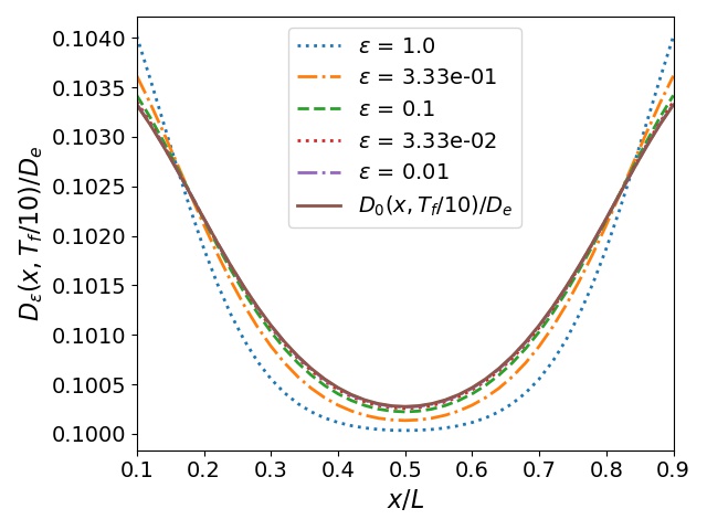
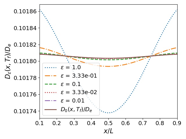
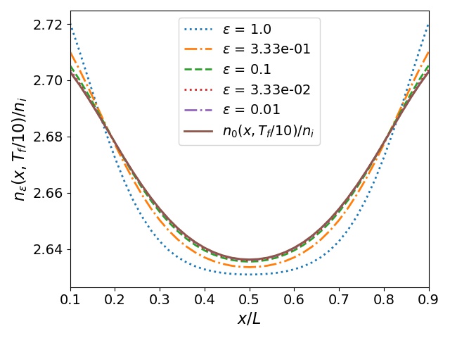
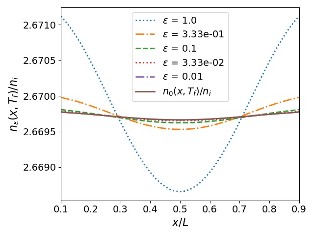
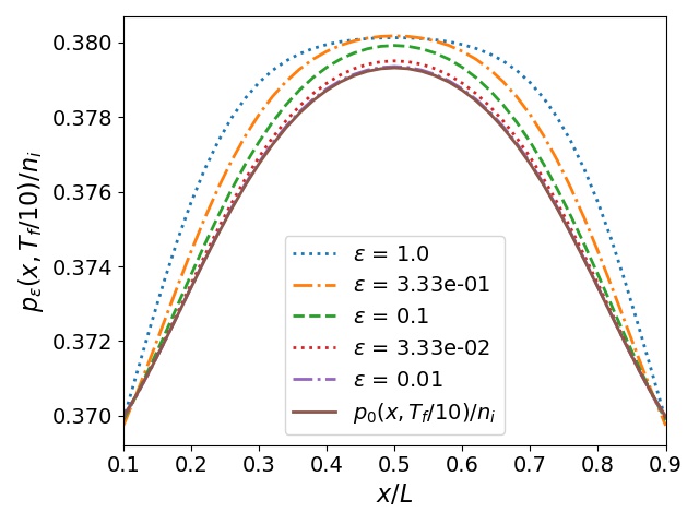
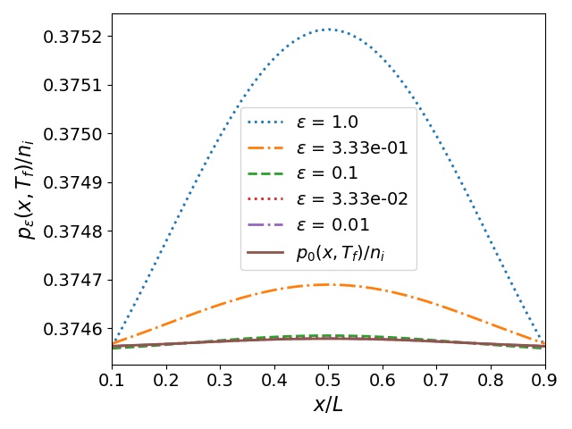
Figure 1. Oxygen vacancy density (top row), electron density (middle row), and hole density (bottom row) versus space at time $t=T_{f}/10$ (left column) and $t=T_{f}$ (right column) for various values of $\varepsilon$ and the reduced problem.

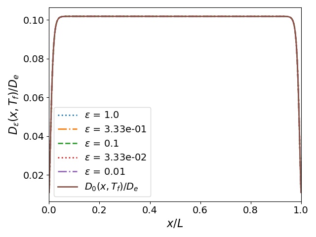
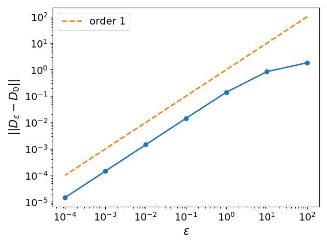
Figure 2. Left: Oxygen vacancy density versus space at time $t=T_{f}$ for various values of $\varepsilon$. Right: Difference of the oxygen vacancy densities $D_{\varepsilon}$ and $D_{0}$ in the $L^{1}(\Omega\times(0,T_{f}))$ norm versus $\varepsilon$.

6.3. Reduced system

In the following, we focus on the reduced system (68)–(69). First, we choose a vanishing applied voltage ($U_{0}=U_{L}=0$) and consider different values for the dopant concentration at the electrode $D_{e}$. Figure 3 (left) shows the spatial distribution of the quotient $D_{0}(x,T_{f})/D_{e}$, where $D_{0}(x,T_{f})$ is close to the steady state. We observe a $U$-shape distribution with a boundary layer near the electrodes. According to [23], the layer comes from the fact that a large vacancy density gradient near the electrode interfaces is required to compensate the strong electrostatic attraction of ions to the image charge on both electrodes. When $D_{e}/D^{I}<1$, the vacancy density decreases away from the electrodes and meet in the center of the device with a vanishing slope, and the shape is inversed when $D_{e}/D^{I}>1$.

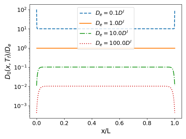
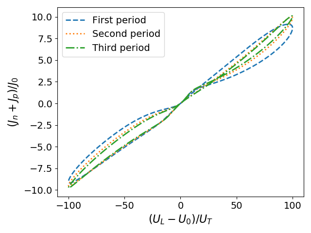
Figure 3. Left: Rescaled vacancy density $D_{0}(x,T)/D_{e}$ for different values of $D_{e}/D^{I}$. Right: Current-voltage characteristics for three periods of a sinuoidal applied voltage.

For the following figure, we fix $D_{e}/D^{I}=10$. Figure 4 shows the zero-bias potential $V(x,T_{f})-V_{\rm bi}-V_{\rm applied}(x)$ and vacancy density at final time $t=T_{f}$ for various applied voltages $U_{L}-U_{0}$, scaled with the thermal voltage $U_{T}=26$ mV. Here, we have set $V_{\rm applied}(x)=(U_{L}-U_{0})(x/L)-U_{0}$. The applied voltage produces a potential barrier for the electrons; it causes the mobile vacancies to drift and results in a complete vacancy depletion at the right side of the device. Similar results have been obtained in [23, Figure 1].

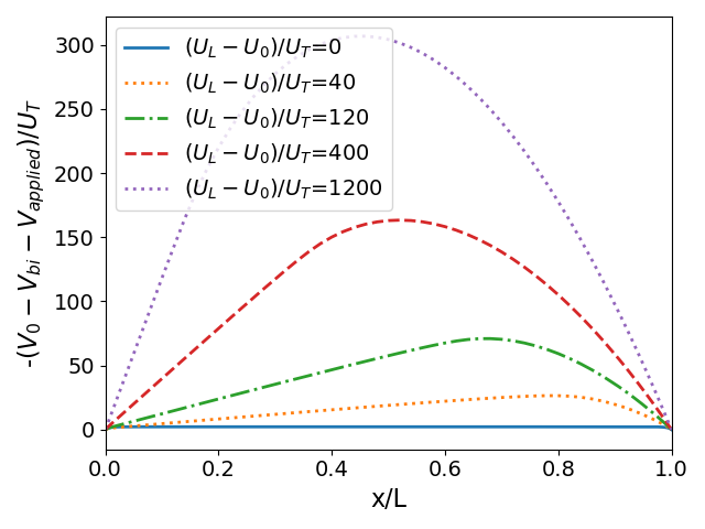
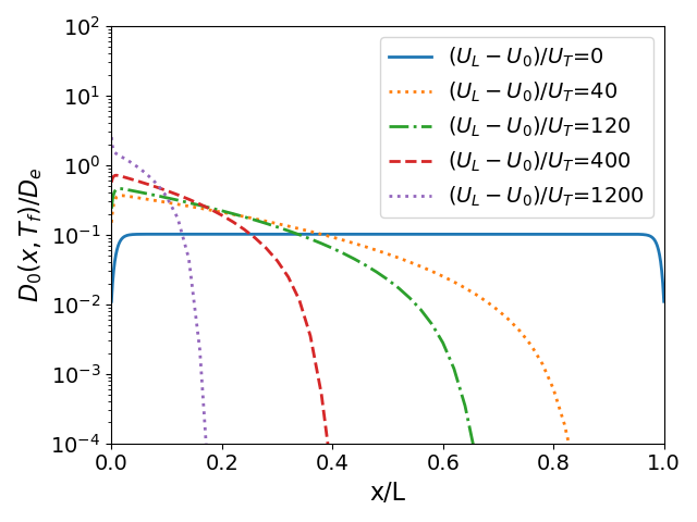
Figure 4. Zero-bias potential $V(x,T_{f})-V_{\rm bi}-V_{\rm applied}$ (left) and oxygen vacancy density $D_{0}(x,T_{f})$ (right) for various applied voltages.

Finally, we consider a sinusoidal applied voltage with $U_{0}=0$, $U_{L}(t)=100\sin(6\pi t/T_{f})$, and $T_{f}=0.03$. The resulting dynamic current-voltage characteristics ($J_{n}(0)+J_{p}(0)$ versus $U_{L}-U_{0}$) are shown in Figure 3 (right). As in [23], we observe a pinched hysteresis loop. This loop is a well-known fingerprint of the ideal memristor introduced in [6]. The same applied potential leads to different current values at different times, which indicates that the device has a memory. This confirms that the drift-diffusion model is able to represent a memristive device.

Appendix A Auxiliary lemmas

Introduce the functions $T_{k}(s)=\min\{k,s\}$ for $s\geq 0$, $k\geq 1$ and

$$g_{k}(s)=\int_{0}^{s}\int_{1}^{y}\frac{dz}{T_{k}(z)}dy,\quad h_{k}(s)=\int_{0}^{s}\frac{dz}{\sqrt{T_{k}(z)}},\quad s\geq 0.$$

Lemma 16.

It holds that $g_{k}(s)=s(\log s-1)$ for $0\leq s<k$ and $g_{k}(s)\geq k(\log k-1)+(s-k)^{2}/(2k)$ for $s\geq k$.

Proof.

We estimate for $0\leq s\leq k$,

$$g_{k}(s)=-\int_{0}^{s}\int_{y}^{1}\frac{dz}{T_{k}(z)}dy=-\int_{0}^{s}\int_{y}^{1}\frac{dz}{z}dy=s(\log s-1);$$

and for $s\geq k$,

$$g_{k}(s)=\int_{0}^{k}\int_{1}^{y}\frac{dz}{T_{k}(z)}dy+\int_{k}^{s}\int_{1}^{y}\frac{dz}{T_{k}(z)}dy\geq k(\log k-1)+\frac{1}{2k}(s-k)^{2},$$

ending the proof. ∎

Lemma 17.

There exists $C>0$ such that for all $k>1$,

$$\sqrt{T_{k}(s)}\leq C\big{(}1+\sqrt{|g_{k}(s)|}\big{)},\quad\sqrt{T_{k}(s)}\leq Ch_{k}(s)\quad\mbox{for }s\geq 0.$$

Proof.

We first prove the inequality $h_{k}(s)^{2}\leq C(1+|g_{k}(s)|)$ and then $\sqrt{T_{k}(s)}\leq h_{k}(s)/2$ for $s\geq 0$. Combining both inequalities shows the lemma. The second inequality follows from

$$h_{k}(s) =\int_{0}^{s}\frac{dy}{\sqrt{y}}=2\sqrt{s}=2\sqrt{T_{k}(s)}\quad\mbox{for }0<s<k,$$

$$h_{k}(s) =\int_{0}^{k}\frac{dy}{\sqrt{y}}+\int_{k}^{s}\frac{dy}{\sqrt{k}}\geq 2\sqrt{k}=2\sqrt{T_{k}(s)}\quad\mbox{for }s\geq k.$$

If $0<s<k$, we have shown in Lemma 16 that $g_{k}(s)=s(\log s-1)$, and then $h_{k}(s)^{2}\leq C(1+|g_{k}(s)|)$ is equivalent to $4s\leq C(1+s|\log s-1|)$ for $0<s<k$, and this inequality is true for a suitable $C>0$. If $s\geq k$, again by Lemma 16, $h_{k}(s)^{2}\leq C(1+|g_{k}(s)|)$ follows from

$$\bigg{(}2\sqrt{k}+\frac{s-k}{\sqrt{k}}\bigg{)}^{2}\leq C\bigg{(}k(\log k-1)+\frac{(s-k)^{2}}{2k}\bigg{)},$$

and this inequality is valid for a suitably chosen $C>0$ independent of $k$. ∎

Let $\xi>0$ and define $g_{\xi}(x)=\xi x(e^{x}-1)$ for $x\geq 0$ and its convex conjugate $g_{\xi}^{*}(y)=\sup_{x>0}(xy-g_{\xi}(x))$ for $y\geq 0$. The following lemma provides an upper bound for $g_{\xi}^{*}$.

Lemma 18.

The convex conjugate function of $g_{\xi}$ can be estimated as

$$g_{\xi}^{*}(y)\leq\xi\frac{(\log(1+y/\xi))^{2}}{1+\log(1+y/\xi)}\bigg{(}1+\frac{y}{\xi}\bigg{)}\quad\mbox{for }y\geq 0.$$

Proof.

For given $y\geq 0$, let $\overline{x}(y)\geq 0$ be the unique solution to $y=g^{\prime}_{\xi}(\overline{x}(y))=\xi(1+\overline{x}(y))e^{\overline{x}(y)}-\xi$. Then

$$g_{\xi}^{*}(y)=\left\{\begin{array}[]{ll}\overline{x}(y)y-g_{\xi}(\overline{x}(y))&\quad\mbox{for }y>g_{\xi}^{\prime}(0)=0,\\ 0&\quad\mbox{for }y=g_{\xi}^{\prime}(0)=0.\end{array}\right.$$

Furthermore, it follows from the definition of $\overline{x}(y)$ that $y/\xi\geq e^{\overline{x}(y)}-1$ and hence, $\overline{x}(y)\leq\log(1+y/\xi)$. Therefore, since $(1+\overline{x}(y))e^{\overline{x}(y)}=1+y/\xi$ by the definition of $\overline{x}(y)$, we have for $y\geq 0$,

$$g_{\xi}^{*}(y) =\overline{x}(y)y-\xi\overline{x}(y)(e^{\overline{x}(y)}-1)=\xi\overline{x}(y)\bigg{(}1+\frac{y}{\xi}-e^{\overline{x}(y)}\bigg{)}$$

$$=\xi\overline{x}(y)\bigg{(}1+\frac{y}{\xi}-\frac{1+y/\xi}{1+\overline{x}(y)}\bigg{)}=\frac{\overline{x}(y)^{2}}{1+\overline{x}(y)}(y+\xi)\leq\frac{(\log(1+y/\xi))^{2}}{1+\log(1+y/\xi)}(y+\xi),$$

which shows the lemma. ∎

We continue with some Gagliardo–Nirenberg (type) inequalities.

Lemma 19 (Gagliardo–Nirenberg).

Let $\Omega\subset{\mathbb{R}}^{d}$ ($d\geq 1$) be a bounded domain with Lipschitz boundary and let $q\leq 2d/(d-2)$ if $d>2$ and $q<\infty$ if $d=2$. Then for all $\delta>0$, there exist $C>0$ and $C(\delta)>0$ such that for all $u\in H^{1}(\Omega)$,

(70) $$\|u\|_{L^{q}(\Omega)} \leq C\|u\|_{H^{1}(\Omega)}^{\theta}\|u\|_{L^{1}(\Omega)}^{1-\theta},$$

(71) $$\|u\|_{L^{q}(\Omega)} \leq\delta\|u\|_{H^{1}(\Omega)}^{\theta}\|u\log|u|\|_{L^{1}(\Omega)}^{1-\theta}+C(\delta)\|u\|_{L^{1}(\Omega)},$$

where $\theta=2d(q-1)/((d+2)q)$. In two space dimensions, we have $\theta=1-1/q$.

Proof.

Inequality (70) is the standard Gagliardo–Nirenberg inequality. Using this inequality, inequality (71) can be proved as in [2, (22)], where the inequality was shown for $q=3$; also see [9, (1.9)]. ∎

We recall the following regularity result, valid in two space dimensions and proved in [12]; also see [9, Lemma 3.1].

Lemma 20 (Regularity for the Poisson equation).

Let $\Omega\subset{\mathbb{R}}^{2}$ satisfy Assumption (A1), and let $v\in H^{1}(\Omega)$ be the unique solution to $\Delta v=f$ in $\Omega$, $v=\overline{v}$ on $\Gamma_{D}$, and $\nabla v\cdot\nu=0$ on $\Gamma_{N}$. There exist $r_{0}>2$ and $C>0$ such that

(72) $$\|v\|_{L^{\infty}(\Omega)} \leq C\big{(}\|f\log|f|\|_{L^{1}(\Omega)}+g(\|v\|_{H^{1}(\Omega)})+1\big{)},$$

$$\|v\|_{W^{1,r_{0}}(\Omega)} \leq C\big{(}\|f\|_{L^{2r_{0}/(r_{0}+2)}(\Omega)}+g(\|v\|_{H^{1}(\Omega)})+1\big{)},$$

where $g$ is a continuous increasing function.

The following lemma follows from the Alikakos iteration method. A proof can be found in [15] for homogeneous boundary conditions. The proof is the same for no-flux and mixed boundary conditions.

Lemma 21.

Let $\Omega\subset{\mathbb{R}}^{d}$ ($d\geq 1$) satisfy Assumption (A1) and let $u^{q/2}\in L^{2}(0,T;H^{1}(\Omega))\cap L^{\infty}(0,T;L^{2}(\Omega))$ for all $q\in{\mathbb{N}}$ with $q\geq 2$ with $u\geq 0$ in $\Omega\times(0,T)$, $u(0)=0$ in $\Omega$, and either $u=0$ on $\Gamma_{D}$, $\nabla u\cdot\nu=0$ on $\Gamma_{N}$, or $u=0$ on $\partial\Omega$, or $\nabla u\cdot\nu=0$ on $\partial\Omega$. Assume that there are constants $K_{0}$, $K_{1}$, $K_{2}>0$ and $\alpha$, $\beta\geq 0$ such that for all $q\geq 2$, $t\in(0,T)$,

$$\int_{\Omega}e^{t}u(t)^{q}dx+K_{0}\int_{0}^{t}\int_{\Omega}e^{s}|\nabla u^{q/2}|^{2}dxds\leq K_{1}q^{\alpha}\int_{0}^{t}\int_{\Omega}e^{s}u^{q}dxds+K_{2}q^{\beta}e^{t}.$$

Then

$$u(t)\leq K_{3}\big{(}\|u\|_{L^{\infty}(0,T;L^{1}(\Omega))}+1\big{)}\quad\mbox{in }\Omega,\ t\in(0,T),$$

where $K_{3}$ depends only on $\alpha$, $\beta$, $d$, $\Omega$, $K_{0}$, $K_{1}$, and $K_{2}$.

References

- [1] C. Bataillon, F. Bouchon, C. Chainais-Hillairet, J. Fuhrmann, E. Hoaraus, and R. Touzani. Numerical methods for the simulation of a corrosion model with moving oxide layer. J. Comput. Phys. 231 (2012), 6213–6231.
- [2] P. Biler, W. Hebisch, and T. Nadzieja. The Debye system: existence and large time behavior of solutions. Nonlin. Anal. 23 (1994), 1189–1209.
- [3] D. Bothe, A. Fischer, and J. Saal. Global well-posedness and stability of electrokinetic flows. SIAM J. Math. Anal. 46 (2014), 1263–1316.
- [4] L. Chen and A. Jüngel. Analysis of a parabolic cross-diffusion population model without self-diffusion. J. Diff. Eqs. 224 (2006), 39–59.
- [5] Y. Choi and R. Lui. Multi-dimensional electrochemistry model. Arch. Ration. Mech. Anal. 130 (1995), 315–342.
- [6] L. Chua. Memristor – The missing electric circuit element. IEEE Trans. Circuit Tech. 18 (1971), 507–519.
- [7] W. Dreyer, P.-E. Druet, P. Gajewski, and C. Guhlke. Analysis of improved Nernst–Planck–Poisson models of compressible isothermal electrolytes. Z. Angew. Math. Phys. 71 (2020), no. 119, 68 pages.
- [8] A. Glitzky, K. Gröger, and R. Hünlich. Free energy and dissipation rate for reaction diffusion processes of electrically charged species. Appl. Anal. 60 (1996), 201–217.
- [9] A. Glitzky and R. Hünlich. Global estimates and asymptotics for electro-reaction-diffusion systems in heterostructures. Appl. Anal. 66 (1997), 206–226.
- [10] A. Glitzky and R. Hünlich. Global existence result for pair diffusion models. SIAM J. Math. Anal. 36 (2005), 1200–1225.
- [11] J. Greenlee, J. Shank, M. Tellekamp, and A. Doolittle. Spatiotemporal drift-diffusion simulations of analog circuit memristors. J. Appl. Phys. 114 (2013), 034504, 9 pages.
- [12] K. Gröger. Boundedness and continuity of solutions to linear elliptic boundary value problems in two dimensions. Math. Ann. 298 (1994), 719–728.
- [13] K. Gröger. Boundedness and continuity of solutions to second order elliptic boundary value problems. Nonlin. Anal. 26 (1996), 539–549.
- [14] A. Heibig, A. Petrov, and C. Reichert. Solvability for a drift-diffusion system with Robin boundary conditions. J. Differ. Eqs. 267 (2019), 2331–2356.
- [15] P. Holzinger and A. Jüngel. Large-time asymptotics for a matrix spin drift-diffusion model. J. Math. Anal. Appl. 486 (2020), no. 123887, 20 pages.
- [16] D. Ielmini and S. Ambrogio. Emerging neuromorphic devices. Nanotech. 31 (2020), 092001, 24 pages.
- [17] A. Jüngel. Transport Equations for Semiconductors. Lecture Notes in Physics 773. Springer, Berlin, 2009.
- [18] A. Jüngel. Entropy Methods for Diffusive Partial Differential Equations. Springer Briefs Math., Springer, 2016.
- [19] A. Jüngel and Y.-J. Peng. A hierarchy of hydrodynamic models for plasmas. Zero-electron-mass limits in the drift-diffusion equations. Ann. Inst. Henri Poincaré, Anal. non lin. 17 (2000), 83–118.
- [20] A. Jüngel. A nonlinear drift-diffusion system with electric convection arising in semiconductor and electrophoretic modeling. Math. Nachr. 185 (1997), 85–110.
- [21] V. Mladenov. Advanced Memristor Modeling. MDPI, Basel, 2019.
- [22] D. Scharfetter and H. Gummel. Large-signal analysis of a silicon Read diode oscillator. IEEE Trans. Electron Devices 16 (1969), 64–77.
- [23] D. Strukov, J. Borghetti, and S. Williams. Coupled ionic and electronic transport model of thin-film semiconductor memristive behavior. Small 5 (2009), 1058–1063.
- [24] M. Verri, M. Porro, R. Sacco, and S. Salsa. Solution map analysis of a multiscale drift-diffusion model for organic solar cells. Computer Meth. Appl. Mech. Engin. 331 (2018), 281–308.
- [25] S. Vongehr and X. Meng. The missing memristor has not been found. Sci. Rep. 5 (2015), 11657, 7 pages.
- [26] H. Wu, T.-C. Lin, and C. Liu. Diffusion limit of kinetic equations for multiple species charged particles. Arch. Ration. Mech. Anal. 215 (2015), 419–441.