Free-Floating Planets, the Einstein Desert, and ’Oumuamua

1 Introduction

The claim by Sumi et al. (2011) of $\sim 2$ Jupiter-mass free-floating planet candidates (FFPs) per star opened up the field of FFP population studies. This led to several works that tried to interpret this population (Clanton & Gaudi, 2014a, b, 2016). However, it was also later contradicted by Mróz et al. (2017), who found no evidence for such planets in a larger sample of events. Both of these studies were limited to statistical analysis of the Einstein timescale ($t_{\rm E}$) distribution, for which the mass dependence is convolved with dependences on the lens-source relative proper motion ($\mu_{\rm rel}$) and lens-source relative parallax ($\pi_{\rm rel}$).

Kim et al. (2021) initiated a new approach to probing the FFP population that focused on analyzing the Einstein radius ($\theta_{\rm E}$) distribution. This approach has two advantages. First, $\mu_{\rm rel}=\theta_{\rm E}/t_{\rm E}$ is automatically determined, which removes one of the two convolutions with unknown distributions that was mentioned above. Second, the selection function is relatively independent of lens mass ($M$) over a broad range of masses.

When Kim et al. (2021) reported KMT-2019-BLG-2073 as the fourth microlensing single-lens event with a measured Einstein radius $\theta_{\rm E}<10\,{\mu\rm as}$, they noted that all four events had giant-star sources, which led them to initiate a long-term study to find all finite-source/point-lens (FSPL) events with such giant-star sources in the 2016-2019 Korea Microlensing Telescope Network (KMTNet, Kim et al. 2016) database. They were motivated in part by the fact that this was the second giant-source FSPL event from 2019 with $\theta_{\rm E}<10\,{\mu\rm as}$, the first being OGLE-2019-BLG-0551 (Mróz et al., 2020). They sought to place these FSPL FFPs in the context of a homogeneously selected sample that would include stars and brown dwarfs (BDs), as well as FFPs. For technical reasons that are briefly reviewed below, they were only able to probe the 2019 database at that time. Their systematic search yielded a total of 13 giant-source FSPL events, including the two FFPs. They carried out a variety of tests and concluded that there was nothing suspicious about the sample. However, they refrained from, and strongly cautioned against, drawing any statistical conclusions from this sample, despite the fact that it was homogeneously selected. They argued that because their study was motivated by noticing two FFP detections in a single year, it could suffer from publication bias.

Two factors prevented (Kim et al., 2021) from carrying out a 4-year search immediately. First, the form of the search had been made possible by a recent upgrade to the 2019 online database, but this had not yet been extended to the previous 3 years. Second, for 2019, Kim et al. (2021) had supplemented their automated analysis of the online database with a special, more aggressive, execution of the EventFinder algorithm (Kim et al., 2018a) that was tailored to giant sources. A more aggressive search was required because the standard EventFinder algorithm takes advantage of the fact that most single-lens/single-source (1L1S) events (and even most binary events) can be qualitatively matched to one of two variants of Gould (1996) 2-parameter profiles. However, this is not the case for typical FFP candidates, for which the source radius, $\theta_{*}$, is often ${\gtrsim}\theta_{\rm E}$, leading to a “top hat” light curve shape. These upgrades and new searches required more than a year of effort.

The search proposed by Kim et al. (2021) was therefore carried out as these steps were completed season-by-season. In the course of this work, Ryu et al. (2021) reported the discovery of KMT-2017-BLG-2820, the third FFP in the KMTNet sample, which by this time was the sixth FSPL FFP overall. That is, in the intervening time, Mróz et al. (2020) had discovered another FFP, OGLE-2016-BLG-1928. Ryu et al. (2021) pointed out that all six FFPs lay below an apparent “gap” in the cumulative $\theta_{\rm E}$ distribution from Figure 9 of Kim et al. (2021), which they dubbed the “Einstein Desert”.

They argued from the definition of $\theta_{\rm E}$,

$$\theta_{\rm E}\equiv\sqrt{\kappa M\pi_{\rm rel}}\qquad\kappa\equiv{4\,G\over c^{2}{\rm AU}}\simeq 8.14\,{{\rm mas}\over M_{\odot}},$$ (1)

that such a desert would be a natural consequence of a bimodal function of the lens mass, $M$. That is, the main stellar and BD lens population in the bulge (with small lens-source relative parallaxes, $\pi_{\rm rel}$) would contribute relatively small Einstein radii, but would be cut off at $\theta_{\rm E}\sim 30\,{\mu\rm as}$ due to a sharp drop in the BD mass function, e.g., near $M\sim 0.02\,M_{\odot}$, combined with the paucity of phase space for $\pi_{\rm rel}{\lesssim}5\,{\mu\rm as}$ (corresponding lens-source relative distances $D_{LS}\equiv D_{S}-D_{L}{\lesssim}300\,{\rm pc}$). Then, a second population of low-mass FFPs, e.g., $M\sim 5\,M_{\oplus}$, with a much higher specific frequency than stars and BDs would give rise to the small-$\theta_{\rm E}$ events.

They then argued that a population of FFPs cannot be in the bulge and produce the observed distribution, because an analogous population in the disk would produce larger-$\theta_{\rm E}$ events that would “fill in” the gap. By contrast, if the small-$\theta_{\rm E}$ events were explained by disk FFPs, an analogous population in the bulge would not be detected. Specifically, for typical giant sources, the very numerous FFPs in the bulge would not give rise to recognizable events because they would induce magnification, $A$, changes of only

$$A-1\simeq{2\over\rho^{2}}={2\kappa M\pi_{\rm rel}\over\theta_{*}^{2}}=0.13\,\biggl{(}{M\over 5\,M_{\oplus}}\biggr{)}\biggl{(}{\pi_{\rm rel}\over 20\,{\mu\rm as}}\biggr{)}\biggl{(}{\theta_{*}\over 6\,{\mu\rm as}}\biggr{)}^{-1}$$ (2)

where $\rho\equiv\theta_{*}/\theta_{\rm E}{\gtrsim}1$. Hence, the FFP events would mainly come from the less numerous disk population. Then, a high inferred specific frequency would be necessary to compensate for the overall relative paucity of disk lenses. (In Section 8, we will show that this reasoning is only partly correct.)

Ryu et al. (2021) recognized that with only 13 FSPL events, the evidence from Kim et al. (2021) for a desert was relatively weak. However, they adduced two additional arguments. First, they noted that the apparent gap was not (yet) contradicted by the ongoing search for FSPL events in 2018 and (part of) 2017 data. Second, they pointed to an analogous desert in the distribution of Einstein timescales,

$$t_{\rm E}\equiv{\theta_{\rm E}\over\mu_{\rm rel}}\qquad\mu_{\rm rel}\equiv|{\mbox{\boldmath$\mu$}}_{\rm rel}|,$$ (3)

found by Mróz et al. (2017) in their analysis of point-source/point-lens (PSPL) events extracted from 5 years of Optical Gravitational Lensing Experiment (OGLE) data. Here, ${\mbox{\boldmath$\mu$}}_{\rm rel}$ is the lens-source relative proper motion. The same argument predicts a desert in the distribution of Einstein timescales, although it is expected to be less pronounced than the one in Einstein radii because the former is a convolution of the proper-motion distribution with the latter.

Thus, this picture gave a coherent account of all available data at that time. Nevertheless, Ryu et al. (2021) counseled a wait-and-see approach. If their hypothesis were correct, they predicted that the Einstein desert would remain relatively parched as new FSPL events were added. If not, one should expect that it would be gradually “filled in”.

Here, we present the full sample of 30 FSPL giant-source events from the KMTNet 2016-2019 database. We find that the Einstein Desert is substantially more distinct than in the 13-event sample from 2019. This strengthens the case for a bimodal mass function, with a broad peak of stars and BDs complemented by a large population of FFPs at much lower masses.

We show that the FFPs are more numerous than the known bound planets. We raise the possibility that the heavier FFPs have mainly been ejected to very wide (rather than unbound) orbits, and may largely be accounted for by the still poorly traced population of very-wide-orbit planets. We also suggest that interstellar asteroids may be the extreme end of the FFP population and, in particular, may follow the same power law.

2 Review of Detection Procedures

The FSPL events reported here are derived from the KMTNet microlensing survey, which uses three identical 1.6m telescopes, each equipped with $2^{\circ}\times 2^{\circ}$ cameras (Kim et al., 2016). The telescopes are located in Chile (KMTC), South Africa (KMTS), and Australia (KMTA). See Figure 12 from Kim et al. (2018a) for the field locations and cadences.

We essentially follow the same procedures for selecting FSPL preliminary candidates as was described by Kim et al. (2021). We refer the reader to that paper for details. Here we give only a brief overview, and we also describe two important differences between their 2019 sample and the 2016-2018 additional events that we present here. One of these was already mentioned by Kim et al. (2021), while the other is new.

We first conduct a purely automated search of the online summary table of KMT events (about 3000 events per year), making use of the impact parameter $u_{0}$, the Einstein timescale $t_{\rm E}$, and the source magnitude $I_{S}$ (from the pipeline Paczyński 1986 PSPL fit), together with the tabulated field extinction $A_{I}$, to impose two selection conditions,

$$I_{S,0,\rm est}\equiv I_{S}-A_{I}<16,$$ (4)

and

$$\mu_{\rm thresh}\equiv{\theta_{*,\rm est}\over u_{0}t_{\rm E}}>1\,{\rm mas}\,{\rm yr}^{-1};$$

$$\theta_{*,\rm est}\equiv 3\,{\mu\rm as}\times 10^{(16-(I_{S}-A_{I}))/5}.$$ (5)

The first condition restricts the sample to giants. On rare occasions, it allows foreground main-sequence or subgiant stars, but these are eliminated at the stage of detailed investigations.

The second condition rejects the great majority of PSPL events while accepting (for further investigation) the overwhelming majority of FSPL events that satisfy Equation (4). First note that the $\theta_{*,\rm est}$ estimate implicitly assumes that the source has a similar color as the clump. This will be approximately so except for stars well up on the giant branch, for which it will be an underestimate. Then, assuming that the online fits for PSPL events (i.e., $\rho<u_{0}$) are approximately accurate, PSPL events will have

$$\mu_{\rm thresh}^{\rm pspl}=0.33\,{{\rm mas}\over{\rm yr}}\biggl{(}{u_{0}\over 1/3}\biggr{)}^{-1}\biggl{(}{t_{\rm E}\over 20\,{\rm day}}\biggr{)}^{-1}\biggl{(}{\theta_{*,\rm est}\over 6\,{\mu\rm as}}\biggr{)}.$$ (6)

Hence, most PSPL giant-source events will fail this criterion, leaving a tractable subset to be rejected by manual light-curve fitting.

On the other hand, for FSPL events, we do not expect the automated fit to yield the correct $u_{0}$. For $\rho\ll 1$, we expect $u_{0,\rm fit}t_{{\rm E},\rm fit}\equiv t_{{\rm eff},\rm fit}\simeq t_{*,\rm true}\equiv\rho_{\rm true}t_{{\rm E},\rm true}$ to the extent that the fit is influenced by the width of the peak, and $1/u_{0,\rm fit}\simeq A_{\rm max,\rm fit}\simeq A_{\rm max,\rm true}\simeq 2/\rho_{\rm true}$ to the extent that the fit is influenced by the height of the peak. These imply $\mu_{\rm rel}\sim\mu_{\rm thresh}$ and $\mu_{\rm rel}\sim\mu_{\rm thresh}/2$, respectively. Hence, FSPL events that fail Equation (5) have relative proper motions $\mu_{\rm rel}{\lesssim}1\,{\rm mas}\,{\rm yr}^{-1}$. Using the approach in the Appendix to Gould et al. (2021), the probability for a lens to have such a small proper motion is $p<(\mu_{\rm thresh}/\sigma_{\mu})^{3}/6\sqrt{\pi}\rightarrow 4\times 10^{-3}$, where we have adopted an isotropic bulge proper-motion dispersion of $\sigma_{\mu}\sim 2.9\,{\rm mas}\,{\rm yr}^{-1}$. Table 4 of Kim et al. (2021), which lists both the estimator $u_{\rm thresh}$ and the true value $\mu_{\rm rel}$ for 13 events shows that the former is conservative in the sense that $\mu_{\rm rel}/\mu_{\rm thresh}{\lesssim}1$. Only two events (OGLE-2019-BLG-0551 and OGLE-2019-BLG-1143) violate this inequality, and they do so only mildly, both with ratios 1.2. Note that neither of the two FFPs in this sample (OGLE-2019-BLG-0551, $\rho=4.5$; KMT-2019-BLG-2073, $\rho=1.1$) are in the $\rho\ll 1$ regime, but both approximately satisfy the inequality, with $\mu_{\rm rel}/\mu_{\rm thresh}=1.2$ and 0.6, respectively.

Each such candidate, typically of order 60 per year, is first reviewed visually. Of order 10% are eliminated at this stage for various reasons, primarily that they are not single lens events or that there are no data near the peak, which would be required to measure $\rho$. The remainder are fitted to PSPL and FSPL forms using pipeline KMT data. If FSPL is preferred by $\Delta\chi^{2}_{\rm fspl}>3$ and the best fit has a normalized impact parameter $z_{0}\equiv u_{0}/\rho<1$ then the data are subjected to tender loving care (TLC) re-reduction. Then, if $\Delta\chi^{2}_{\rm fspl}>20$, the event is selected as FSPL. For a few cases, the pipeline light curve has an obvious FSPL form for which PSPL would give a very poor fit. For these, we move directly from inspection to TLC. Note that both the pipeline reductions and TLC reductions use pySIS (Albrow et al., 2009), which is a specific implementation of difference image analysis (Tomaney & Crotts, 1996; Alard & Lupton, 1998).

For 2019, Kim et al. (2021) separately searched the output of the real-time event selection algorithm AlertFinder (Kim et al., 2018b) and the end-of-year selection algorithm EventFinder (Kim et al., 2018a). Because AlertFinder did not operate in the wings of the season and also because it searches only for rising events, there were wing-of-season events that it missed but were found by EventFinder. However, even in the region of overlap, there were FSPL events that were missed by one or the other. For example the FFP FSPL event OGLE-2019-BLG-0551 was found by AlertFinder but not EventFinder. These discrepancies motivated the addition of an aggressive giant-source search, which had two purposes. First, it served as a check that the union of the AlertFinder and EventFinder samples for 2019 was effectively complete. And, indeed, the special giant-source search did not yield any additional FSPL events. However, Kim et al. (2021) also noted that 2019 was the first year for which AlertFinder was in full operation. For 2018, AlertFinder operated only beginning in June and only in the northern bulge. It did not operate at all in 2016 and 2017. Hence, given that EventFinder was missing FSPL events in 2019, the special giant-source search would have to be applied to previous seasons. See Ryu et al. (2021) for further refinements of the giant-source search.

Finally, we modified the search procedures relative Kim et al. (2021) to better deal with saturated data. In 2019, events that were saturated at peak were simply eliminated as uninterpretable at the visual-inspection stage. However, we subsequently realized that many such events could be analyzed by incorporating the $V$-band data for the regions of the light curve that were saturated in the $I$ band. For example, given the typical intrinsic colors of giants $(V-I)_{0}\sim 1.1$, typical reddening of KMT fields $E(V-I)\sim 1.8$ and the roughly 0.65 deeper photometric zero point in the $V$ band, the onset of saturation would be $\sim(1.1+1.8-0.65)=2.25$ mag fainter in the $V$ band than the $I$ band. Of course, $V$-band data were taken 10 times less frequently in 2017-2019 than $I$ band, and even less frequently in 2016. However, for events that are well characterized by bright (so, generally small-error) $I$-band light curves, only a few points are needed over peak to measure $\rho$. We applied this approach to the saturated events from 2019, but this did not lead to new FSPL events. However, it did prove useful in fully characterizing FSPL events from 2016-2018.

3 Expected $\theta_{\rm E}$ Distribution

Our primary motivation is to probe the poorly understood population of FFPs. To do so, it is useful to understand the $\theta_{\rm E}$ distribution that is expected from stars and BDs. We first show that a substantial majority of these detections will come from bulge lenses and second that these are expected to cover the range $30\,{\mu\rm as}{\lesssim}\theta_{\rm E}{\lesssim}300\,{\mu\rm as}$. We then turn to the role of disk lenses.

Ignoring selection effects, the rate of microlensing events for a population of fixed mass $M$ and toward a given source is

$$\Gamma_{\rm all}\propto\int\mu_{\rm rel}\theta_{\rm E}(D_{L})D_{L}^{2}dD_{L}\nu f(\mu_{\rm rel})\mu_{\rm rel}g(M;D_{L}),$$ (7)

where $\nu=\nu(D_{L})$ is the density at distance $D_{L}$, $f(\mu)=f(\mu_{\rm rel};D_{L})$ is the 1-dimensional proper motion distribution and $g(M,D_{L})$ is the mass function. However, for FSPL events, we replace $\theta_{\rm E}(D_{L})\rightarrow\rho\theta_{\rm E}(D_{L})=\theta_{*}$, which eliminates one instance of implicit dependence on $D_{L}$ (and $M$; Gould & Yee 2013). We note that with the exception of very nearby lenses $D_{L}{\lesssim}1\,{\rm kpc}$ (see below), the mean proper motion $\langle\mu_{\rm rel}\rangle$ is approximately independent of distance, while we also approximate $g(M)$ as being independent of distance. Hence, for FSPL events,

$$\Gamma_{\rm FSPL}\propto\theta_{*}\langle\mu_{\rm rel}\rangle g(M)\int_{D_{L}=0}^{D_{S}}dD_{L}D_{L}^{2}\nu(D_{L}).$$ (8)

That is, $\Gamma_{\rm FSPL}$ is proportional to the total column of lenses in the observation cone between the observer and the bulge source. Without any detailed model, it is clear that this column is dominated by bulge lenses: otherwise, e.g., there would be a cloud of disk clump stars trailing toward brighter magnitudes from the observed bulge clump on the color-magnitude diagram (CMD). Hence, bulge stars will dominate most of the $\theta_{\rm E}$ distribution, while disk lenses will dominate only in regions that are inaccessible to bulge lenses.

The bulge mass function is well populated over the range $0.02\,M_{\odot}{\lesssim}M{\lesssim}1\,M_{\odot}$. The upper limit is set by the fact that the bulge is primarily an old population for which the stars that were born $M{\gtrsim}1\,M_{\odot}$ have now mainly evolved to become remnants, mostly white dwarfs. The lower limit is an approximation for the steeply falling mass function in the BD regime. The bulge has a depth of order $1\,{\rm kpc}$, implying that the typical range of lens-source relative parallaxes is $0.005\,{\rm mas}{\lesssim}\pi_{\rm rel}{\lesssim}0.02\,{\rm mas}$, corresponding to lens-source separations $0.35\,{\rm kpc}{\lesssim}(D_{S}-D_{L}){\lesssim}1.5\,{\rm kpc}$. Above the upper limit, the product of the disk and bulge density distribution declines sharply. Below the lower limit, the amount of available phase space declines. None of the four limits just described is a hard boundary, but together they indicate a well-populated range, for $\theta_{\rm E}=\sqrt{\kappa M\pi_{\rm rel}}$ of $30\,{\mu\rm as}{\lesssim}\theta_{\rm E}{\lesssim}400\,{\mu\rm as}$.

Then, we should consider whether these intrinsic boundaries are impacted by additional detection effects. For typical giant-star source radii $\theta_{*}\sim 6\,{\mu\rm as}$, these limits correspond to $A_{\rm max}\sim 2/\rho\sim 10$ and 135, respectively. The lower limit is not near any selection boundary, but saturation becomes an issue at the upper limit. For typical giant sources $I_{0}\sim 14.5$ and extinctions $A_{I}\sim 2$, the upper boundary implies $I_{\rm peak}\sim 11.2$, which is well into the range of KMT saturation, whose onset is seeing (and hence observatory) dependent. As we discussed in Section 2, it is sometimes possible to recover from saturation using $V$-band data. Nevertheless, the onset of saturation steepens the decline in the upper range of $\theta_{\rm E}$ detections, leading us to adopt $30\,{\mu\rm as}{\lesssim}\theta_{\rm E}{\lesssim}300\,{\mu\rm as}$ as the expected range for bulge lenses.

If we were to adopt a similar mass function for disk lenses, then they would populate a range that is translated upward by a factor $\sqrt{\pi_{{\rm rel},\rm disk}/\pi_{{\rm rel},\rm bulge}}\sim 2$ in $\theta_{\rm E}$, where we have adopted $\pi_{{\rm rel},\rm disk}\sim 60\,{\mu\rm as}$ and $\pi_{{\rm rel},\rm bulge}\sim 15\,{\mu\rm as}$ as “typical” values for the disk and bulge, respectively. Hence, the disk lenses would appear as “sprinkled in” (and not generally individually identifiable) over the range $60\,{\mu\rm as}{\lesssim}\theta_{\rm E}{\lesssim}400\,{\mu\rm as}$, and they would only start to dominate for $\theta_{\rm E}{\gtrsim}400\,{\mu\rm as}$. The fact that the disk mass function extends above $M{\gtrsim}M_{\odot}$ augments this effect but does not qualitatively change it. As just mentioned, this high $\theta_{\rm E}$ regime is suppressed by saturation effects. However, another way to express the relation of the disk and bulge contributions is that at fixed $\theta_{\rm E}$, the disk lenses have $\sim 4$ times lower mass than the bulge lenses. Hence, at $\theta_{\rm E}\sim 400\,{\mu\rm as}$, they are near the peak of the mass function $M\sim 0.3\,M_{\odot}$, whereas the bulge lens mass function at $M\sim 1\,M_{\odot}$ is much lower. Hence, we expect that, contrary to the main part of the $\theta_{\rm E}$ distribution, the upper range will be a comparable mix of disk and bulge lenses.

Table 1: Microlens Parameters for FSPL giant-star events

Name	KMT Name	$t_{0}$	$u_{0}$	$t_{\rm E}$	$\rho$	$f_{s,\rm KMTC}$
OB180705	KB181882	8316.30592	0.00123	46.247	0.01151	5.5354
	(errors)	0.00145	0.01239	0.147	0.00503	0.0187
KB180244	KB180244	8312.42231	0.27149	4.430	0.35487	11.0566
	(errors)	0.00118	0.00301	0.027	0.00283	0.1300
OB180626	KB182309	8230.28800	0.16989	2.983	0.21484	10.3031
	(errors)	0.00132	0.00255	0.024	0.00251	0.1520
MB17147	KB170132	7850.99388	0.09138	2.695	0.13451	4.3062
	(errors)	0.00043	0.00097	0.016	0.00102	0.0393
OB171254	KB170374	7952.25224	0.00000	15.278	0.02527	0.7068
	(errors)	0.00025	0.00000	0.046	0.00009	0.0024
OB170560	KB172830	7859.52120	0.02900	0.901	0.89000	18.5140
	(errors)	0.00100	0.01800	0.002	0.00300	0.0010
OB170905	KB171022	7895.73816	0.08702	7.734	0.15031	83.4744
	(errors)	0.00401	0.00221	0.046	0.00254	0.9971
MB17241	KB170818	7883.47648	0.21697	1.845	0.29496	4.8304
	(errors)	0.00057	0.00437	0.024	0.00483	0.1019
OB170084	KB170726	7807.13435	0.01226	43.642	0.02335	0.4049
	(errors)	0.00212	0.00022	0.501	0.00028	0.0055
OB161045	KB160848	7559.20148	0.01061	12.030	0.02943	1.3546
	(errors)	0.00115	0.00208	0.099	0.00191	0.0141
KB161128	KB161128	7486.32769	0.00951	12.550	0.02586	0.2703
	(errors)	0.00147	0.00105	0.428	0.00105	0.0106
OB161540	KB162262	7606.72400	0.60500	0.330	1.63100	19.6960
	(errors)	0.00100	0.02700	0.003	0.00800	0.0000
KB162057	KB162057	7467.93171	0.00000	11.374	0.06645	2.4595
	(errors)	0.00196	0.00000	0.105	0.00078	0.0309
MB16258	KB160606	7537.29800	0.18800	3.722	0.57400	49.7270
	(errors)	0.00100	0.00400	0.045	0.00300	0.4670

Notes: The units of $t_{0}$ and $t_{\rm E}$ are HJD${}^{\prime}={\rm HJD}-2450000$ and days, respectively. Fluxes are in units of an $I=18$ system. Event names are abbreviations for, e.g., OGLE-2018-BLG-0705. For KB172820, see Ryu et al. (2021). For OB170896 (=KB170799), see Shvartzvald et al. (2019). For OB171186 (=KB170357), see Li et al. (2019). For OB180705, the fit included parallax: $(\pi_{{\rm E},N},\pi_{{\rm E},E})=(-0.324,-0.017)\pm(0.139,0.008)$.

Table 2: CMD and Derived Parameters for FSPL giant-star events

Name	KMT Name	$(V-I)_{0}$	$I_{0}$	$\theta_{*}$	$\theta_{\rm E}$	$\mu_{\rm rel}$	$\mu_{\rm thresh}$	$z_{0}=u_{0}/\rho$
OB180705	KB181882	1.46	13.14	14.78	1285.00	10.10	13.31	0.104
KB180244	KB180244	2.26	12.06	34.25	96.72	7.97	7.79	0.764
OB180626	KB182309	1.20	14.69	6.53	29.00	3.55	5.63	0.791
MB17147	KB170132	0.94	14.18	6.22	46.24	6.26	13.75	0.679
KB172820	KB172820	1.13	14.31	7.05	5.94	7.95	10.34	0.150
OB171254	KB170374	1.27	14.97	5.68	224.11	5.35	10.14	0.000
OB170896	KB170799	1.26	14.95	5.71	139.60	3.42	5.94	0.115
OB170560	KB172830	2.43	12.47	31.10	34.90	14.17	5.80	0.033
OB170905	KB171022	1.60	11.19	38.50	256.15	12.09	5.49	0.579
MB17241	KB170818	1.24	14.29	7.65	25.93	5.13	5.09	0.736
OB171186	KB170357	2.12	12.39	26.90	93.90	2.65	2.88	0.319
OB170084	KB170726	1.33	15.41	4.78	204.11	1.71	2.38	0.525
OB161045	KB160848	1.23	14.37	7.33	249.31	7.55	43.72	0.360
KB161128	KB161128	1.00	14.43	5.49	212.79	6.19	24.10	0.368
OB161540	KB162262	1.70	13.58	14.36	8.80	9.74	8.80	0.371
KB162057	KB162057	1.20	14.58	7.29	109.71	3.52	8.41	0.000
MB16258	KB160606	2.92	12.31	43.89	76.45	7.50	1.65	0.328

Notes: The units of $\theta_{*}$ and $\theta_{\rm E}$ are ${\mu\rm as}$, while those of $\mu_{\rm rel}$ and $\mu_{\rm thresh}$ are ${\rm mas}\,{\rm yr}^{-1}$. Event names are abbreviations for, e.g., KMT-2018-BLG-1882, OGLE-2018-BLG-0705, and MOA-2017-BLG-147

We note that the higher proper motions of nearby lenses $D_{L}{\lesssim}1\,{\rm kpc}$ do not compensate for their low observing-cone volume in the rate equation. The mean proper-motion term in this regime scales $\langle\mu_{\rm rel}(D_{L})\rangle\sim v_{\perp,\rm typ}/D_{L}$ where $v_{\perp,\rm typ}\sim 40\,{\rm km}\,{\rm s}^{-1}\sim 8\,{\rm kpc}\,{\rm mas}\,{\rm yr}^{-1}$ is the typical transverse velocity of nearby stars. Hence, when the proper-motion term is moved inside the integral, it takes the form $v_{\perp,\rm typ}\int dD_{L}\,D_{L}\ldots$ in place of $\langle\mu_{\rm rel}\rangle\int dD_{L}\,D_{L}^{2}\ldots$ at larger distances. That is, the nearby lens contribution is still heavily suppressed by the volume factor.

Finally, it is reasonable to expect sensitivity to FSPL events with peak magnifications down to $A_{\rm max}\sim 2$, i.e., $\rho\sim 1.4$ (Equation (2), hence $\theta_{\rm E}\sim\theta_{*}/1.4\sim 4\,{\mu\rm as}$. Thus, the survey should have sensitivity that goes almost a decade below the Einstein radii that are generated by known stars and BDs.

4 30 FSPL Events from 2016-2019

Table 1 shows the microlens fit parameters for the 14 of the 17 new FSPL events that were discovered in 2016-2018 data. The parameters for the remaining three are adopted from previous publications. See Appendix A. For the 13 FSPL events from 2019, see Table 3 of Kim et al. (2021).

For the color-magnitude analysis, we used the same procedures as Kim et al. (2021), ultimately based on Yoo et al. (2004). Briefly, we perform a special reduction using pyDIA (Albrow, 2017), which carries out light-curve photometry and field-star photometry on the same system. We find $I_{S}$ by regression of the $I$-band light curve on the best model and the $(V-I)_{S}$ color by regression of the $V$-band on the $I$-band light curve. We find the clump centroid of the field stars, and so calculate the offset $\Delta[(V-I),I]$ of the source relative to the clump. We estimate the intrinsic clump color $(V-I)_{\rm cl,0}=1.06$ from Bensby et al. (2013) and its intrinsic magnitude $I_{\rm cl,0}$ from Table 1 of Nataf et al. (2013). We convert from $V/I$ to $V/K$ using the color-color relations of Bessell & Brett (1988). Finally, we estimate $\theta_{*}$ using the color/surface-brightness relations of Kervella et al. (2004) for K giants and Groenewegen (2004) for M giants. The results of the CMD analysis are shown in Table 2 for the 17 events from 2016-2018. For the 13 FSPL events from 2019, see Table 4 of Kim et al. (2021).

Among the 17 newly reported FSPL events, we recovered the FFP OGLE-2016-BLG-1540 (Mróz et al., 2019) (and, as already reported by Ryu et al. 2021, the FFP KMT-2017-BLG-2820), but did not find any additional FFPs. Hence, there are a total of four FFPs in the sample of 30 FSPL events, OGLE-2016-BLG-1540, KMT-2017-BLG-2820, OGLE-2019-BLG-0551, and KMT-2019-BLG-2073.

We did not recover either of the other two known FSPL FFPs, OGLE-2012-BLG-1323 (Mróz et al., 2019) and OGLE-2016-BLG-1928 (Mróz et al., 2020). The first preceded the KMT survey. For the second, the event was not found either by EventFinder nor in the special giant-source search because there are only 4 magnified KMT points. Even if identified, it could not have been reliably characterized from these four points. OGLE’s original identification of this event was post-season and was based on 10 magnified points that probe both the peak and the wings. The role of KMT data (in addition to confirming the event from KMTC) was to rule out binary models by the flat behavior of KMTS data starting about 8 hours after the last OGLE point.

In Appendix A, we provide notes on individual events.

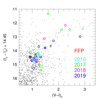
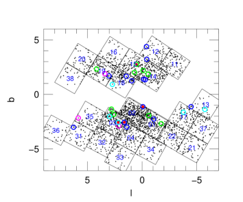
Figure 1: Color-magnitude locations of the 30 FSPL events relative to the clump, shown against a background of field stars from the CMD of KMT-2019-BLG-2555, i.e., the same as was used in Figure 8 of Kim et al. (2021). The events are color-coded by discovery year. FFPs have red cores. As expected, the sources are concentrated in the clump (the highest concentration of giants), are somewhat over-represented on the upper giant branch (due to larger cross sections), and, conversely somewhat under-represented on the lower giant branch. The largest outlier, OGLE-2017-BLG-0905 (green point near top), is discussed in Appendix A, while the second largest, KMT-2019-BLG-1143 (blue point toward the right), was discussed by Kim et al. (2021). The lack of detections with ordinate ${\gtrsim}15.5$ is discussed in Section 5, with reference to Kim et al. (2021).

Figure 2: Field positions of 30 FSPL events in Galactic coordinates, color-coded accorded to year of discovery (see labels in Figure 2). The background black points are (as in Figure 4 of Kim et al. 2021) EventFinder events from 2019. As in that Figure, the KMT fields are shown as black squares, with blue field numbers. Their observational cadences can be obtained from Figure 12 of Kim et al. (2018a).

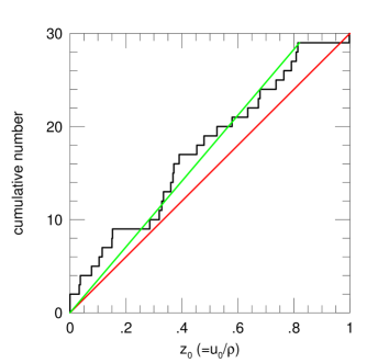
Figure 3: Cumulative distribution of normalized impact parameters $z_{0}=u_{0}/\rho$. The red line connects the first and last points, while the green line connects the first and penultimate points. The underlying distribution is rigorously uniform in $z_{0}$, so the eye is struck by the absence of detections toward $z_{0}\simeq 1$. According to a Kolmogorov-Smirnov (KS) test, this is not significant, but the effect may be real because the KS test does not capture all the physics. See Section 5. The distribution relative to the green line suggests that the sample is homogeneously selected for $z_{0}{\lesssim}0.8$.

Figure 4: Cumulative Distribution of $\log\theta_{\rm E}$ for 30 FSPL events with giant-star sources that were found in four seasons of KMTNet data, 2016-2019. The absence of detections $\theta_{\rm E}{\lesssim}4\,{\mu\rm as}$ is due to selection effects, while the paucity for $\theta_{\rm E}{\gtrsim}300\,{\mu\rm as}$ is due to a combination of selection effects and the lack of bulge stars $M{\gtrsim}1\,M_{\odot}$. The remaining feature, the factor $\sim 3$ “Einstein Desert”, $8.8\,{\mu\rm as}<\theta_{\rm E}<26\,{\mu\rm as}$, is the signature of two populations, i.e., BDs/stars with masses $0.02{\lesssim}M/M_{\odot}{\lesssim}1$ to the right and FFPs with much lower masses to the left. The former are detected mainly in the bulge, while the latter are likely to be about equally drawn from the bulge and the disk. See Section 8.3. This Figure can be compared to Figure 10 from Kim et al. (2021).

5 Sample Characteristics

Notwithstanding the justified caution of Kim et al. (2021), the results from 2019 prove to be reasonably representative of the four year sample. For the four years 2016-2019, the FFP/FSPL counts are (1/5, 1/9, 0/3, 2/13). For 2016-2018, they are 2/17 compared to 2/13 for 2019, which is consistent with normal Poisson variations. If four detections are distributed randomly among four seasons, the most common configuration (144/256) is the observed one, (2,1,1,0). The one feature that is possibly unusual is that there were only 3 FSPL events in 2018 compared to 13 in 2019, so one may wonder whether the seasonal distribution of FSPL events, $n_{i}=(5,9,3,13)$ can also be considered as a “typical” outcome of Poisson sampling. We investigate this by adopting an annual expectation $\lambda=30/4=7.5$ and construct a log likelihood $\ln L=\sum_{i=1}^{4}\ln(e^{-\lambda}\lambda^{n_{i}}/n_{i}!)=-10.31$. We can then compare this to the same statistic for $10^{6}$ realizations in which 30 events are randomly distributed among 4 seasons. We find that 7.8% have smaller likelihood. Thus, this outcome is not particularly “unexpected”, especially given that this is a posterior test. Therefore, neither the seasonal distribution of the FFPs nor that of the FSPL events can be considered unusual.

Kim et al. (2021) presented several diagnostic plots whose purpose was to probe for statistical artifacts and/or patterns in the sample and to identify individual outliers that might require explanation and/or further investigation. We present analogous plots here.

Figure 2 shows the color-magnitude diagram (CMD) source positions of the FSPL events relative to the clump, color-coded by season. The blue (2019) points and the black background points (taken from the dereddened CMD of KMT-2019-BLG-2555) are the same as those shown in Figure 8 of Kim et al. (2021). Of the 30 sources, 15 are clump stars (or giant-branch stars that are superposed on the clump), 4 are lower-giant-branch stars, 9 track the upper giant branch quite closely, one (KMT-2019-BLG-1143, blue) lies significantly below the upper giant branch, and one (OGLE-2017-BLG-0905, green) lies well above the upper giant branch.

The broad pattern of the FSPL events relative to the background is as expected: they are concentrated in the clump (i.e., the most densely populated region of giant stars), and are somewhat over-represented on the upper giant branch and under-represented on the lower giant branch, which is expected due to larger and smaller cross sections, respectively. The complete absence of FSPL events between $16<I<15.5$ would appear to be somewhat surprising. However, Kim et al. (2021) showed that this is due to systematic underestimation (with considerable scatter) of source flux for FSPL events by the automated pipeline. See their Figure 7.

The outlier KMT-2019-BLG-1143 was investigated by Kim et al. (2021). We investigate the other outlier (OGLE-2017-BLG-0905) in Appendix A.

Figure 2 shows the distribution of the 30 FSPL events on the sky in Galactic coordinates, against the same background of 2019 EventFinder events that appears in Figure 4 of Kim et al. (2021). The FSPL events are concentrated toward the Galactic plane, as would be expected for giant-source events because they are more heavily represented in regions of high extinction. However, this is a weak effect, and no strong statistical conclusion can be drawn from this apparent pattern.

Figure 3 shows the cumulative distribution of the 30 FSPL events as a function of normalized impact parameter $z_{0}\equiv u_{0}/\rho$. In nature, this distribution is exactly uniform, so any (statistically significant) deviation from a uniform distribution should reflect selection effects. Kim et al. (2021) had argued based on their analogous Figure 3, that the distribution was consistent with being uniform over $[0\leq z_{0}<1]$. Comparison of the observed distribution with a uniform expectation (red line) indicates that, with accumulating statistics, this may no longer be true. A Kolmogorov-Smirnov (KS) test yields an unimpressive $p=28\%$. However, KS is a very “forgiving” test because it assumes no prior information on the form of the deviation. By contrast, our eye is drawn to the near absence of events with $z_{0}>0.82$, where we might expect the greatest difficulty for detections. The green line, which ignores the single detection at $z_{0}\simeq 1$, appears more satisfying. Kim et al. (2021) argued that there is substantial information about $\rho$ in the regions of the light curve having $z\equiv u/\rho>1$, so that uniform sensitivity over $[0\leq z_{0}<1]$ was plausible. However, it is also plausible that there would be at least some effect for $z_{0}\sim 1$, as seems to be indicated by Figure 3, albeit weakly.

One might suspect that the dearth of events with $z_{0}\sim 0.9$ is the result of the $z_{0}<1$ boundary in our initial selection combined with ordinary statistical noise. That is, some events with initial estimates $z_{0,\rm init}\sim 0.9$ were ultimately eliminated after they were determined to have $z_{0,\rm TLC}>1$ from subsequent TLC reductions, but the “complementary” events that would have had $z_{0,\rm TLC}\sim 0.9$ (if TLC reductions had been done) were not investigated after it was found that $z_{0,\rm init}>1$. In fact, we were concerned about this and obtained TLC for 5 events with $z_{0,\rm init}{\gtrsim}1$. However, $z_{0,\rm TLC}>1$ was confirmed for all 5. Hence, we do not believe that such selection bias is a strong effect.

6 The Einstein Desert

Figure 4 shows the cumulative distribution $\log\theta_{\rm E}$ for the 30 FSPL events in the survey. It exhibits three principal features; 1: a paucity of detections with $\theta_{\rm E}{\gtrsim}300\,{\mu\rm as}$, 2: a complete absence of detections with $\theta_{\rm E}<4\,{\mu\rm as}$, and 3: the “Einstein Desert”, i.e., the absence of detections over the interval, $8.8\,{\mu\rm as}<\theta_{\rm E}<26\,\theta_{\rm E}$.

As discussed in Section 3, the first was expected, primarily due to the rapid fall-off of the bulge mass function for $M{\gtrsim}1\,M_{\odot}$, but somewhat augmented by selection effects due to saturation. The latter will be examined more closely in Section 7.

As will also be discussed in Section 7, the second feature is likewise due to selection.

However, selection effects play no role in the third feature, the “Einstein Desert”, because the selection function is smoothly increasing from a factor of 2 below the Desert to a factor of a few above it.

As was already anticipated in Section 3, the upper shore of this desert (at $\theta_{\rm E}=26\,{\mu\rm as}$) can be attributed to the sharp fall-off in the bulge mass function in the BD regime. In this sense, it is qualitatively similar to the first feature, but with a crucial difference. Being generated by a fall-off at the high end of the mass function, the first feature is “washed out” by contributions of disk lenses of much lower mass (hence, higher specific frequency) but with similar $\theta_{\rm E}=\sqrt{\kappa M\pi_{\rm rel}}$. By contrast, the population of disk stars and BDs only contribute to $\theta_{\rm E}$ in regions well above the desert, and so the upper edge of the Desert is sharp.

The 4 events that lie below the Desert must represent a separate, low-mass population because they have Einstein radii that are a factor ${\gtrsim}3$ below those of the lowest-mass bulge BD lenses (and even farther below those of the lowest-mass disk BD lenses). The existence of the Desert is a powerful constraint on the nature of this population: whatever model one adopts must not only reproduce the observed low-$\theta_{\rm E}$ detections but must also respect the absence of such detections in the Desert.

Figure 6 shows a scatter plot of FSPL proper motions against Einstein radii. Generally, the proper motions are consistent with those expected for bulge and disk lenses. Note that the FFPs are within this range, somewhat more tightly grouped but with a median similar to the sample as a whole.

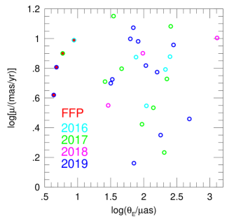
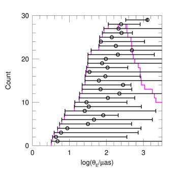
Figure 5: Scatter plot of $\log\mu_{\rm rel}$ vs. $\log\theta_{\rm E}$ for the 30 FSPL giant-source events from four years of KMTNet data. The events are color coded by year: cyan (2016), green (2017), magenta (2018), and blue (2019). The four FFPs at the left (with red interiors) all have $\mu_{\rm rel}>4\,{\rm mas}\,{\rm yr}^{-1}$, whereas the 26 non-FFPs are distributed more broadly. However no strong conclusion can be drawn from this. Note that Figure 9 of Kim et al. (2021) corresponds to the blue points in this Figure.

Figure 6: Measurements (circles) and sensitivity limits (error bars) of $\theta_{\rm E}$ for 29 FSPL events, rank ordered by lower limits. As the $\theta_{\rm E}$ of hypothetical events is progressively reduced below that of the actual event, it eventually falls below the detection threshold, either because $\Delta\chi^{2}_{\rm select}<1000$ (required to detect the event) or $\Delta\chi^{2}_{\rm fspl}<20$ (required to be chosen as an FSPL event). As $\theta_{\rm E}$ is progressively increased, the peak of the event eventually saturates, making it impossible to measure $\theta_{\rm E}$. KMT-2019-BLG-2528 with $\Delta\chi^{2}_{\rm select}=973$ is excluded because the detection itself fails $\Delta\chi^{2}_{\rm select}>1000$. The magenta histogram shows the number of FSPL events that were sensitive to each $\theta_{\rm E}$.

7 Selection Effects

7.1 Selection Effects Due to Lens Mass (thus, $\theta_{\rm E}$)

There are two principal selection effects due to lens mass that can prevent a given event from entering the sample. These derive from the requirements that, first, the light curve must initially be selected as a “microlensing event”, and second, that finite source effects must be detected in this event. In Section 2, we adopted a threshold for finite source effects: $\Delta\chi^{2}_{\rm fspl}\equiv\chi^{2}({\rm PSPL})-\chi^{2}({\rm FSPL})>20$. The threshold for event detection, $\Delta\chi^{2}_{\rm select}$, i.e., the difference in $\chi^{2}$ between microlensing and non-microlensing interpretations of the light curve as determined by EventFinder and the special giant-star searches, varied somewhat for different subsamples (see Kim et al. 2021). For purposes of this section, we impose the minimum threshold that was common to all subsamples, namely, $\Delta\chi^{2}_{\rm select}>1000$. This has the effect of eliminating one of the FSPL events from the sample, i.e., KMT-2019-BLG-2528 with $\Delta\chi^{2}_{\rm select}=973$. A hypothetical event can drop out of the sample either because $\Delta\chi^{2}_{\rm fspl}$ falls below our threshold of 20 or because $\Delta\chi^{2}_{\rm select}$ falls below our threshold of 1000. Under our assumptions for real versus hypothetical events, we will see that both $\Delta\chi^{2}_{\rm fspl}$ and $\Delta\chi^{2}_{\rm select}$ will monotonically decline with falling mass.

To understand how selection effects impact these two criteria, consider two events that are “identical” in every respect except for the lens mass, e.g., a real event and a hypothetical event with either larger or smaller lens mass. Here, “identical” means that the lens and source of the hypothetical event both have the same 6 phase-space coordinates as the real event and that the source radius and temperature are also the same. Under these assumptions, $\mu_{\rm rel}$, $z_{0}=u_{0}/\rho$, $t_{*}=\rho t_{\rm E}$, and $t_{\rm eff}=u_{0}t_{\rm E}$ are the same for the two events. However, because $\theta_{\rm E}$ scales as $M^{1/2}$, $t_{\rm E}$, $u_{0}$, and $\rho$ all differ. Specifically, $t_{\rm E}\propto M^{1/2}$, $u_{0}\propto M^{-1/2}$, and $\rho\propto M^{-1/2}$. We also assume that the observational sequences of the real and hypothetical events are the same. Then, we can evaluate upper and lower limits on $\theta_{\rm E}$ for each real event based on comparison to hypothetical events under these assumptions.

First consider the case that the real and hypothetical events satisfy $\rho_{\rm real}<\rho_{\rm hyp}\ll 1$, i.e., in particular, $M_{\rm hyp}<M_{\rm real}$. Then, because $z_{0}$ is the same in both cases, both the PSPL and FSPL models will have essentially the same morphologies in the peak region of each event. In addition, because the duration of the transit, $\Delta t_{\rm trans}=2t_{\rm E}\sqrt{\rho^{2}-u_{0}^{2}}$, is invariant, they will have roughly the same number of data points over the peak region. On the other hand, they will have a magnification ratio $A_{\rm hyp}/A_{\rm real}\simeq(\rho_{\rm hyp}/\rho_{\rm real})^{-1}=\theta_{{\rm E},\rm hyp}/\theta_{{\rm E},\rm real}$. Hence, the real event will be brighter than the hypothetical one, and the number of “signal photons” (difference between the true number for the FSPL model and the expected number for the incorrect PSPL model) will fall linearly with $\theta_{{\rm E},\rm hyp}$, while the number of background photons remains the same. Hence, $\Delta\chi^{2}_{\rm fspl}$ will fall linearly with $\theta_{{\rm E},\rm hyp}$ if the hypothetical event is “above sky” and quadratically if it is “below sky”. Once $\theta_{\rm E}$ falls sufficiently that $\rho{\gtrsim}1$, the functional forms of the models in the two cases start to differ, but the principle remains the same. We estimate $\Delta\chi^{2}_{\rm fspl}$ by scaling to the actual value found from the FSPL and PSPL fits to the real data and calculating the signal-to-noise ratio of each case by assuming typical $2^{\prime\prime}$ FWHM seeing and a typical $I$-band background of 19.25 mag per square arcsec.

Next we turn to $\Delta\chi^{2}_{\rm select}$. As long as $\rho{\lesssim}1$, the principal impact of declining $\theta_{\rm E}$ on $\Delta\chi^{2}_{\rm select}$ is that $t_{\rm E}$ is shorter, so that there are fewer magnified data points for a given event. Hence, $\Delta\chi^{2}_{\rm select}$ declines as $\Delta\chi^{2}_{\rm select}\propto t_{\rm E}\propto\theta_{\rm E}$. Eventually, $\theta_{\rm E}$ becomes small enough that $\rho\gtrsim 1$, at which point, finite source effects dominate the morphology of the light curve. At this point, the effect of the further decline of $\theta_{\rm E}$ through $\rho=1$ on $\Delta\chi^{2}_{\rm select}$ is similar to that on $\Delta\chi^{2}_{\rm fspl}$.

On the other hand, as the mass is increased, eventually the peak flux $f_{\rm peak}\simeq 2f_{s}/\rho\propto M^{1/2}$ will grow so large that the images become saturated over peak. As discussed above, in many cases it will still be possible to measure $\rho$ from the $V$-band images. However, these are 10 times less frequent, and so for low-cadence fields they may not sample the peak region. Moreover, as the mass continues to be raised, eventually the $V$-band images will also become saturated. We model this process by assuming the same seeing and background as above, and by reducing $\Delta\chi^{2}$ by a factor 20 for the regime in which $I$ is saturated but $V$ is not. Here, a factor 10 comes from the lower cadence in $V$ band and 2 comes from the lower photon counts in the $V$ band. This sets an upper limit on the detectable $\theta_{\rm E}$ for a given event.

In most cases, we do not actually know the lens mass, but we do know $\theta_{*}$ and $\theta_{\rm E}$. Hence, we can still compare the real and hypothetical events in terms of a measurable quantity, $\theta_{\rm E}=\theta_{*}/\rho$. Then, for each event $i$, with measured Einstein radius, $\theta_{{\rm E},i}$, there is some range $\theta_{{\rm E},\min,i}<\theta_{\rm E}<\theta_{{\rm E},{\rm max},i}$ over which it could have been detected, where $\theta_{{\rm E},\min,i}<\theta_{{\rm E},i}$ is set by the $\Delta\chi^{2}$ threshold (either $\Delta\chi^{2}_{\rm fspl}$ or $\Delta\chi^{2}_{\rm select}$) and $\theta_{{\rm E},{\rm max},i}>\theta_{{\rm E},i}$ is set by saturation.

Figure 6 shows these ranges of sensitivity to $\theta_{\rm E}$ for the 29 FSPL events with $\Delta\chi^{2}_{\rm select}>1000$, rank ordered by the $\theta_{{\rm E},\min}$ of each event. The most important feature of this Figure is that the 4 lowest-$\theta_{\rm E}$ events (i.e., the 4 FFPs) are all pressed up near their detection limit. By contrast, and with one very telling exception, there is no such effect for the highest-$\theta_{\rm E}$ events. For example, the 8 events with $\theta_{\rm E}>200\,{\mu\rm as}$ occupy a broad range of positions relative to the detection limits for that event. This suggests that the fact that there is only one event with $\theta_{\rm E}>500\,{\mu\rm as}$ is due to the low frequency of such events in nature rather than lack of sensitivity of the survey. Indeed, as shown by the magenta curve, of the 29 FSPL events, 22 would be able to detect events with $\theta_{\rm E}=500\,{\mu\rm as}$. Moreover, there is a well-understood reason for the paucity of $\theta_{\rm E}{\gtrsim}500\,{\mu\rm as}$ events: as discussed in Section 3, these are almost entirely due to disk lenses, and in a mass range for which the mass function is already in decline. Indeed, the one event that lies above this limit (OGLE-2018-BLG-0705), is known to lie far in the foreground $D_{L}\sim 2.5\,{\rm kpc}$ by two independent arguments. First, it has a measured $\pi_{\rm E}$ (in addition to the known $\theta_{\rm E}$), yielding $\pi_{\rm rel}=\theta_{\rm E}\pi_{\rm E}$. Second, its Gaia proper motion indicates that it is a member of NGC 6544, whose distance is well-determined by several techniques. See Appendix A. Hence, the fact that the low-$\theta_{\rm E}$ events are all pressed up against the detection limit hints that these may represent the “edge” of a population that we are just barely detecting.

7.2 Selection Effects Due to $\mu_{\rm rel}$

There are also selection effects due to lens-source relative proper motion. To understand these, we consider hypothetical events with the same $\theta_{\rm E}$ and lens-source trajectory, but moving with faster or slower proper motion. For hypothetical proper motions that are higher, the hypothetical event will be “sped up” ($t_{\rm E}$, $t_{\rm eff}$, and $t_{\star}$ will all be shorter) compared to the real one, so $\Delta\chi^{2}_{\rm select}$ and $\Delta\chi^{2}_{\rm fspl}$ will both fall inversely as $\mu_{\rm rel}^{-1}$, and so will eventually fall below our thresholds of selection and/or detection. On the other hand, as $\mu_{\rm rel}$ is decreased, the event will be “slowed down”, thus reducing $\mu_{\rm thresh}$ in direct proportion, i.e., $\mu_{\rm thresh}\propto\mu_{\rm rel}$. Thus, it will eventually fall below our search limit of $\mu_{\rm thresh}>1\,{\rm mas}\,{\rm yr}^{-1}$. Our main concern here will be the proper-motion selection effects for the 4 FFPs. These have $\theta_{\rm E}=(4.35,4.77,5.94,8.80)\,{\mu\rm as}$, $\mu_{\rm rel}=(4.17,6.14,7.95,9.74)\,{\rm mas}\,{\rm yr}^{-1}$, $\mu_{\rm thresh}=(3.46,11.17,10.34,8.80)\,{\rm mas}\,{\rm yr}^{-1}$, $\Delta\chi^{2}_{\rm select}=(2180,2663,2992,6249)$, and $\Delta\chi^{2}_{\rm fspl}=(577,234,187,1513)$. Therefore, they have, respectively, $\mu_{{\rm rel},\min}=(1.21,0.55,0.77,1.11)\,{\rm mas}\,{\rm yr}^{-1}$ and $\mu_{{\rm rel},{\rm max}}=(9.09,16.35,23.79,60.87)\,{\rm mas}\,{\rm yr}^{-1}$. The lower limits play very little role, but the upper limits will be important when evaluating the kinematic constraints on the FFP masses (see Section 8).

8 Constraints on the FFP Population

If the “Einstein Desert” is real, then it implies that the objects that lie below this gap are a separate population of low-mass objects. The existence of this gap will then be an important constraint on the mass function of these objects. Hence, the first question that must be addressed is, how statistically secure is this gap?

8.1 Is the Einstein Desert Real?

The fact that the eye is drawn to the gap in Figure 4 does not, in itself, make it real. We can construct the following “naive test” by noting that there are 4 detections within a factor of 2 below the gap, and 6 within a factor of 2 above it. Given that the sensitivity of the survey is monotonically increasing over this entire range and that the gap itself covers a factor of 3, we would expect a continuous distribution to generate $(4+6)/2\times\log(3)/\log(2)=7.9$ detections in the region of the gap. The fact that none are detected has a formal probability of $p=0.0004$. However, we call this test “naive” because it is constructed after the fact. The above statistical evaluation would be valid only if we asked the question before conducting the experiment. We might have asked a dozen questions, such as: is there a gap around $\theta_{\rm E}\sim 15\,{\mu\rm as}$, around $30\,{\mu\rm as}$ etc. Or perhaps the data would have yielded some other peculiar feature, causing us to construct some other posterior test designed to highlight its improbability. If we could imagine constructing 50 such tests, then the probability of finding $p=0.0004$ in one of them is 2%. This is still small but the case would not be overwhelming.

Nevertheless, the fact is that we did not enter this investigation without any prior knowledge. Mróz et al. (2017) already found an analogous gap in the Einstein timescale distribution at $t_{\rm E}\simeq 0.5\,$days. At typical lens-source relative proper motions $\mu_{\rm rel}\sim 7\,{\rm mas}\,{\rm yr}^{-1}$ (for disk lenses), we would expect a gap at $\theta_{\rm E}=\mu_{\rm rel}t_{\rm E}\sim 10\,{\mu\rm as}$, which is similar to the geometric center of the gap in Figure 4: $15\,{\mu\rm as}$. Hence, the above statistical test should be taken approximately at face value. That is, we regard the suggestion by Mróz et al. (2017) of a new population as confirmed.

8.2 $\delta$-Function FFP Mass Function

When Sumi et al. (2011) and Mróz et al. (2017) first suggested their respective FFP populations, they each presented their frequency estimates in terms of $\delta$-function mass functions. Neither argued that the FFP mass function was sharply peaked, but rather used $\delta$-functions as a convenient way to characterize the basic mass scale and frequency. In Section 8.3, we will argue that, especially in light of the Einstein radius measurements presented here, power laws provide a more useful framework to characterize FFPs. However, there is one constraint on the FFP mass function that is most easily described in terms of $\delta$-functions, namely, that the observed FFP proper motions put a lower limit on the FFP mass scale.

As noted in the discussion of Figure 6, the observed distribution is consistent with that of typical disk lenses. Strictly speaking, however, this really applies only to disk lenses with $D_{L}{\gtrsim}2\,{\rm kpc}$ for which the component of the proper motion that is due to the peculiar motion of the lenses (relative to Galactic rotation) is small compared to the mean relative proper motion that is set by the proper motions of the bulge sources. For $D_{L}{\lesssim}1\,{\rm kpc}$, by contrast, these peculiar motions dominate, and the expected amplitude of the relative proper motion grows $\mu_{\rm rel}\propto D_{L}^{-1}$ with declining distance. Hence, at sufficiently low $M$ (hence, low $D_{L}$), the observed “typical disk” proper motions of the FFPs should come into strong tension with what is expected for nearby lenses.

We quantify this conflict as follows. For each assumed lens mass $M$, and for each of the four FFP events, we calculate $\pi_{\rm rel}=\theta_{\rm E}^{2}/\kappa M$. We adopt $\pi_{S}$ from Nataf et al. (2013) and so find $D_{L}={\rm AU}/(\pi_{\rm rel}+\pi_{S})$, and we adopt ${\mbox{\boldmath$\mu$}}_{S,{\rm hel}}$ from Gaia. We model the disk as having a flat rotation curve with $v_{\rm rot}=235\,{\rm km}\,{\rm s}^{-1}$. We model the disk lenses as having velocity dispersions $\sigma_{l}=28\,{\rm km}\,{\rm s}^{-1}\sqrt{\eta}$ and $\sigma_{b}=18\,{\rm km}\,{\rm s}^{-1}\sqrt{\eta}$, where $\eta=\exp(D_{L}/2.5\,{\rm kpc})$, and we assume an asymmetric drift of $v_{\rm rot}-\sqrt{v_{\rm rot}^{2}-(18^{2}+28^{2}+33^{2})\eta\,({\rm km}\,{\rm s}^{-1})^{2}}$. We conduct a 2-dimensional integral over this velocity distribution, first calculating ${\mbox{\boldmath$\mu$}}_{{\rm rel},{\rm hel}}$ and than converting to ${\mbox{\boldmath$\mu$}}_{\rm rel}$. At that point, we exclude realizations that exceed the upper limits that are described in Section 7 for each event. And, of course, we weight the result by $\mu_{\rm rel}$. We find the fraction of this predicted $\mu_{\rm rel}$ distribution that have proper motions less than the observed values, $g_{i}$. For a fair sample, we expect that the $g_{i}$ should be uniformly distributed, with mean $\langle g_{i}\rangle=1/2$, but if the model is systematically overestimating the proper motions (i.e., it assumes that the lenses are closer than they actually are), then we expect $g_{i}\ll 1/2$. Hence we adopt a likelihood estimator $L=\prod_{i=1}^{4}g_{i}$. We find that FFPs with $M<1.5\,M_{\oplus}$ are disfavored at $2\,\sigma$, while those with $M<0.95\,M_{\oplus}$ are ruled out at $3\,\sigma$. These limits correspond to mean lens distances of 1.1 kpc and 0.7 kpc, respectively. That is, these results conform to our naive expectation.

Thus, any compact mass function (not necessarily a $\delta$-function) for which the expected detections were $M{\lesssim}M_{\oplus}$ would be heavily disfavored. However, as we will see explicitly in Section 8.3, only a small fraction of expected detections from viable power-law distributions are in this range.

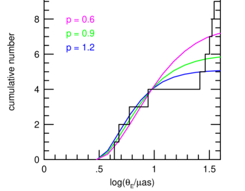
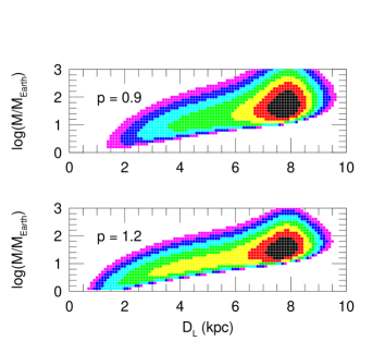
Figure 7: Cumulative distributions of FFP detections for three power-law indices (colored curves) compared to the actual detections (black). The curves are each normalized to 4 detections at Einstein radius $\theta_{\rm E}=9\,{\mu\rm as}$. The three curves then predict (3,1.5,1) detections within the observed Einstein Desert for $p=(0.6,0.9,1.2)$, which argues strongly that the index is steeper than the measured one for bound planets, $\gamma=0.6$.

Figure 8: Relative number of FFP detections predicted for $p=0.9$ and $p=1.2$ power-law distributions, as a function of distance from the Sun and FFP mass. The contours represent steps of a factor 1.5. For $p=1.2$, the larger area in yellow and green almost perfectly compensates the lower amplitude compared to the smaller black region, so that the FFPs are predicted to come equally from the bulge and the disk. For $p=0.9$ the ratio is bulge:disk = 5:4.

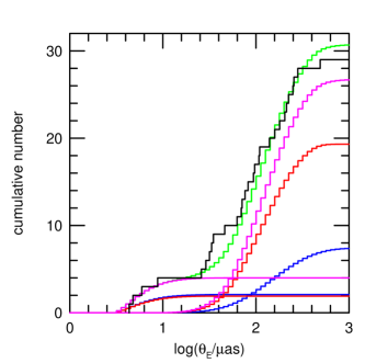
Figure 9: Cumulative distribution of predicted FSPL detections (colored curves) versus the actual detections (black) of 29 events. The FFP model ($p=1.2$), which flattens for $\log(\theta_{\rm E}/{\mu\rm as}){\gtrsim}1.2$, is normalized to 4 detections, shown as disk (blue), bulge (red), and combined (magenta) curves. The same three colors are used for the predictions for stars and BDs, which start to rise at $\log(\theta_{\rm E}/{\mu\rm as})\sim 1.2$. The star+BD normalization is set so that the overall prediction (green) matches the observed profile.

8.3 Power-Law FFP Mass Function

The FFP mass function is likely to be better characterized by a power-law function,

$${dN\over d\log M}=Z\times\biggl{(}{M\over M_{\rm norm}}\biggr{)}^{-p},$$ (9)

than a $\delta$-function. Like the latter, a power-law function requires two parameters, namely the power-law index $p$ and the normalization $Z$, while the reference mass $M_{\rm norm}$ is an arbitrary zero point whose inclusion allows $Z$ to have simple units; i.e., (dex)^-1. The first argument favoring a power-law distribution is that there is no reason to expect that FFPs will have special mass scale, only that selection biases may possibly “pick out” FFPs of a certain scale. Second, FFPs are very likely to be related in some way to bound planets, whose mass-ratio function is very well characterized by a power law. For lenses with an observed $\theta_{\rm E}$, the inferred mass varies as a function of distance, $M=\theta_{\rm E}^{2}/\kappa\pi_{\rm rel}$, with $\pi_{\rm rel}={\rm AU}(D_{L}^{-1}-D_{S}^{-1})$, and so can be very different if the lenses are assumed to be in the disk or bulge. Only a continuous mass distribution (of which, a power-law function has the simplest form) can handle these possibilities simultaneously.

Moreover, we do in fact have some prior information on the power-law index $p$. For planets in the mass range under consideration, $M<M_{\rm Saturn}$, it is difficult to imagine any formation scenario other than within the disks around stars, i.e., the same process that gives rise to the known population of bound planets found by microlensing planet searches. These have a power-law mass-ratio distribution, $dN/d\log q\propto q^{-\gamma}$, with $\gamma\simeq 0.6$ (Jung et al., in preparation, Zang et al., in preparation, Suzuki et al. 2016, Shvartzvald et al. 2016). The FFPs must either be drawn from this population and ejected to larger and/or unbound orbits, or they must form in the outer portions of their solar system, i.e., beyond the range of detection of the known bound population. In either case, we would expect this to result in a mass distribution with $p>\gamma$. That is, the probability for a planet drawn from the known bound population to be scattered to a large or unbound orbit monotonically increases with declining mass because this generally requires scattering off a heavier planet. And planets formed in the outer disk (by core-accretion rather than gravitational collapse) should be heavily biased toward low mass because of the paucity of raw material and the long dynamical timescales. For example, in our own Solar System only dwarf planets such as Pluto are believed to have formed in situ in the outer Solar System, while Uranus and Neptune are believed to have formed inside the current orbit of Saturn and to have been scattered to their present-day orbits.

In the observed mass-ratio function for bound planets, the number of planets with mass ratio greater than a certain $q$, is $\propto q^{-\gamma}$. Then, assuming that scattering to large or unbound orbits is proportional to the number of such potential scatterers, $p=k\gamma$, with $k=2$. In practice, heavier planets will be more efficient scatterers, which would imply $1<k<2$. On the other hand, if the number of FFPs is of order or larger than the number of bound planets (as seems to be the case, see Section 9.2), then the original value of $\gamma$ must have been larger than currently observed, with lower mass members of the original bound population having been preferentially removed. In this case, the present-day observed mass ratio distribution (and, in particular, its power-law form) must reflect the imprint of the scattering process in addition to the formation process. However, because the FFP population is not overwhelmingly dominant, it is unlikely that taking account of formation-plus-scattering can drive $k$ much above the range $1<k<2$.

Starting from these very general considerations, we ask whether and how the FSPL FFP sample can further constrain $p$. Figure 8 shows the predicted cumulative distribution of FFPs based on the range of power laws described above, $p=(0.6,0.9,1.2)$, corresponding to $k=(1,1.5,2)$. In making these predictions we have adopted relative detection efficiencies ${\cal E}=(4/3)X$ $(X<0.5)$, ${\cal E}=(2X+1)/3$ $(0.5<X<1)$, ${\cal E}=1$ $(1<X<2)$, ${\cal E}=2-X$ $(2<X<3)$, with $X\equiv\log(\theta_{\rm E}/3\,{\mu\rm as})$. In the regime $X>0.5$, in which the detections are roughly randomly distributed in the range of detectability (Figure 6), this function approximates the relative fraction of events that are sensitive to a given $\theta_{\rm E}$. For $X<0.5$, we complete this function linearly by imposing a threshold at $\theta_{\rm E}=3\,{\mu\rm as}$, which is supported by the fact that all four FFPs are pressed up close to this limit.

The curves are all normalized to the 4 detections with $\theta_{\rm E}<9\,{\mu\rm as}$. As can be seen, all three curves account of the form of the detections very well. However, they then predict, respectively, about 3, 1.5, and 1 event in the Einstein Desert. Hence, they are, respectively, strongly disfavored, mildly disfavored, and acceptable.

In Figure 8 we show the predicted distribution of detections as a function of FFP mass and distance for the latter two models. The contours change color at factors of 1.5. The bulge FFPs are centered at $M\sim(40,30)\,M_{\oplus}$ for $p=(0.9,1.2)$, while the disk FFPs are at a broad range of lower masses, as expected from the facts that $\theta_{\rm E}$ is measured for the objects in our sample and $M=\theta_{\rm E}^{2}/\kappa\pi_{\rm rel}$. As we will soon see, there are almost exactly the same number of bulge and disk FFPs in the $p=1.2$ model: the fact that the yellow and green contours are much larger than the black contour compensates for their 2.2–3.4 times lower amplitude. For the $p=0.9$ model, we find that the ratio is bulge:disk = 5:4.

To normalize this distribution we predict the stellar and brown-dwarf FSPL events using a Chabrier initial mass function (with bulge stars that have $M>1\,M_{\odot}$ being converted into remnants). See Figure 9. We normalize the FFP curves to 4 total detections and normalize the stellar curve to approximately match the observed distribution. The bulge and disk FSPL events are shown in red and blue respectively, with magenta showing the sum of these. There are two sets of such curves, one for FFPs and the other for stars and BDs. The green curve shows the overall sum. For the FFPs, the bulge and disk curves are almost identical. As noted above, for the $p=0.9$ model, the bulge FFPs would be favored 5:4. From the relative normalization of the FFP and star-plus-BD curves, the FFP mass function can be expressed as

$${dN\over d\log M}={0.39\over{\rm dex\times star}}\times\biggl{(}{M\over 38\,M_{\oplus}}\biggr{)}^{-p},\ \quad(p=0.9\ {\rm or}\ 1.2).$$ (10)

Because the mean mass of the adopted stellar-BD mass function is $\langle M\rangle=0.199\,M_{\odot}$, this can also be written

$${dN\over d\log M}={1.96\over{\rm dex}\times M_{\odot,\rm stars}}\times\biggl{(}{M\over 38\,M_{\oplus}}\biggr{)}^{-p}.$$ (11)

The uncertainty in the normalization is strongly dominated by the Poisson error of 4 FFP detections, i.e., it is 50%. We consider that it is unlikely that the power-law index lies far outside the indicated range $0.9{\lesssim}p{\lesssim}1.2$. For indices much below $p=0.9$, the FFPs would populate the Einstein Desert. While there are no strong constraints on power laws that are substantially steeper than $p=1.2$, it is hard to imagine a mechanism that would generate them.

Assuming that these power laws apply to FFPs from Earth to Saturn masses, then this range contains a total of $130\,M_{\oplus}$ or $200\,M_{\oplus}$ of FFPs per solar mass of stars for the $p=0.9$ and $p=1.2$ models, respectively.

We note that the form of the bulge and disk stellar FFP detections shown in Figure 9 are in reasonable accord with the expectations of Section 3. The observed FSPL events are above the expectations in the BD regime. This may reflect an underestimation of the BD component in the Chabrier mass function, but it could also reflect a statistical fluctuation. Addressing this question would take us beyond the scope of the present investigation.

9 Discussion: Relation of FFPs to Known Populations

When we introduced the acronym “FFP”, we were careful to have it refer to “candidates”, rather than just “free-floating planets”. The main reason for this is the general concern that the low-mass objects that appear “isolated” in microlensing events could be bound planets in orbits that are too wide to enable microlensing signatures of the host. This possibility has always been recognized and was explored in depth by Clanton & Gaudi (2014a, b, 2016). Gould (2016) pointed out that the orbital separations of FFPs in very wide (“Kuiper-like”) and extremely wide (“Oort-like”) orbits could eventually be measured.

Here, we compare the FFP population as derived from our FSPL survey, as characterized by Equations (10) and (11) to various known populations, in order to obtain a more comprehensive picture. This will include planets discovered by microlensing in typical orbits, known planets in very wide orbits, and known interstellar objects.

We adopt the orientation that the most likely origin of FFPs is that they they formed within a factor of a few of the snow line, a region that was rich in proto-planetary materials, and where dynamical timescales were relatively short, and that they were ejected by dynamical processes, either to much wider orbits or to unbound orbits. Hence, we regard it as likely that FFPs comprise both bound and unbound objects. Within this framework, we expect a greater fraction of high-mass FFPs to be in bound orbits, simply because it is easier to eject a test particle than an object whose mass is a substantial fraction of that of the perturber.

9.1 Comparison to Mroz et al. (2017)

Mróz et al. (2017) considered a $\delta$-function model with FFP mass $M=5\,M_{\oplus}$ to account for their $N_{t_{\rm E}}=6$ short-$t_{\rm E}$ events. They obtained a best fit of $R_{5\,M_{\oplus},t_{\rm E}}=10$ FFPs per star. Although they did not quote an error in this estimate, the Poisson noise yields $\sigma_{5\,M_{\oplus},t_{\rm E}}=R_{5\,M_{\oplus},t_{\rm E}}/N_{t_{\rm E}}^{1/2}=4.1$.

To compare our result to theirs, we insert the same $\delta$-function model into the formalism described in Section 8.3, thereby obtaining $R_{5\,M_{\oplus},\theta_{\rm E}}=15.3\pm 7.6$, based on our $N_{\theta_{\rm E}}=4$ small-$\theta_{\rm E}$ detections. Hence, the two determinations are consistent at the $0.6\,\sigma$ level.

Although we mainly restrict consideration to our own results in this work, we note that, because the two normalizations are consistent, it can also be appropriate to combine them. We then find that the combined normalization is a factor

$$F_{\rm renorm}=0.73\pm 0.24$$ (12)

smaller compared to results from our study alone. Note that the fractional error is then $\simeq 1/3$ rather than 1/2, as would be expected from the fact that there are a total of 10 detections, rather than 4. Note also that this renormalization would apply to both Equations (10) and (11) and to either indicated power-law index.

9.2 Comparison to the Known Bound-planet Mass-ratio Function

At present, the masses of most microlensing planets are unknown. Hence, what is most precisely measured is the planet-host mass-ratio ($q$) function, which can be expressed, in analogy to Equation (9),

$${dN\over d\log q}=Z_{q}\times\biggl{(}{q\over q_{\rm norm}}\biggr{)}^{-\gamma},$$ (13)

which, using a zero point $q_{\rm norm}=10^{-3.5}$, has measured values $Z_{q}=0.175\,({\rm dex})^{-2}$/star and $\gamma=0.6$ (Jung et al. 2022, in preparation, Zang et al. 2022, in preparation). There are three things that make the comparison difficult. First, the units of $Z$ are $({\rm dex})^{-1}/$star while the units of $Z_{q}$ are $({\rm dex})^{-2}/$star. The additional “dex” means “per decade of projected separation”. We account for this by regarding two decades of separation (roughly 0.1–10 ${\rm AU}$) as being approximately representative of the whole population. That is, we roughly account for not only the cold planets detected by microlensing but also the hot and warm planets detected by transit and radial velocity surveys. Second, the denominator term “star” does not mean exactly the same thing for the two power-law functions. For our FSPL study, events enter the sample in proportion to their number density, but for the mass-ratio functions studies of Jung et al. (in preparation) and Zang et al. (in preparation), they enter as microlensing events, whose frequency is weighted by their cross section, i.e., $\propto M^{1/2}$. Therefore, if we want to convert Equation (13) to “per solar mass of stars”, we should calculate the mean mass weighted by $M^{1/2}$, i.e., $\langle M\rangle_{\sqrt{M}}\simeq 0.33\,M_{\odot}$. Third, eponymously, the argument of the mass function is mass, while the argument of the mass-ratio function is mass ratio. We account for this by evaluating at bound-planet mass $m_{p}=q\langle M\rangle_{\sqrt{M}}$. With these approximations, we infer a frequency of known bound planets of

$${dN\over d\log m_{p}}={1\over{\rm dex}\times M_{\odot,{\rm stars}}}\times\biggl{(}{m_{p}\over 38\,M_{\oplus}}\biggr{)}^{-0.6}.$$ (14)

Comparison of Equations (11) and (14) indicates that at the normalization mass there are 2 times more FFPs than bound planets, while at lower masses, the ratio is even larger. For example, at $m_{p}=10\,M_{\oplus}$, it is about 3 for the $p=0.9$ power law. Of course, this comparison required several approximations due to the intrinsic incommensurablity of the underlying measurements. Nevertheless, one can infer robustly that the number of FFPs is of order or larger than the number of bound planets in the mass range to which the FFP measurement is directly sensitive, $5{\lesssim}M/M_{\oplus}{\lesssim}60$ (see Figure 8). This implies, as foreshadowed in Section 8.3, that the form of the bound-planet mass function was shaped partly, or perhaps mainly, by the ejection process, rather than just the formation process.

9.3 Comparison to Known Uranus- and Neptune-like Planets

In the entire Universe, there are exactly three known planets that can be securely described as “Uranus-like” ( or “Neptune-like”), in that their masses and separations are of the same order as these two planets, namely, Uranus and Neptune themselves, as well as OGLE-2008-BLG-092Lb, which has $s=5.3$ and $q=2.4\times 10^{-4}$ (Poleski et al., 2014).

9.3.1 Uranus and Neptune

We focus first on Uranus and Neptune. Equation (11) predicts that, for $p=0.9$ and within a factor $\sqrt{10}$ of $M=(M_{\rm Uranus}+M_{\rm Neptune})/2=16\,M_{\oplus}$, each solar mass of stars should be accompanied by an average 4.3 FFPs (whether unbound or in wide orbits). This can be compared to the two such observed planets in the Solar System, the only planetary system for which we have a complete census. These numbers are compatible within the Poisson error, and they would be more so if we applied the renormalization given by Equation (12), by which the expectation would be reduced to $3.1\pm 1.0$.

Furthermore, if a doppelganger of the Solar System gave rise to a microlensing event at $D_{L}\sim 5\,{\rm kpc}$ in which either its “Uranus” or its “Neptune” generated a characteristic FSPL profile, there is only a small chance that its “Sun” would leave a trace on the event. That is, if a planet lies at (3-dimensional) physical separation from its host, $r$, then the probability that its normalized projected separation, $s$, and host-source impact parameter, $u_{0}$, lie within specified regimes are,

$$p(s<s_{{\rm max}})=1-\sqrt{1-{s^{2}\over s_{\rm full}^{2}}},\qquad p(u_{0}<u_{0,{\rm max}})={u_{0}\over s_{\rm full}},$$ (15)

where $s_{\rm full}\equiv r/D_{L}\theta_{\rm E}$. We note that for $D_{L}=5\,{\rm kpc}$ and $D_{S}=8\,{\rm kpc}$, $D_{L}\theta_{\rm E}=3.91\,{\rm AU}(M/M_{\odot})^{1/2}$, but for the entire range, $2.5\,{\rm kpc}<D_{L}<5.5\,{\rm kpc}$, this formula remains accurate to $<4\%$. Thus, for Uranus and Neptune doppelgangers, $s_{\rm full}=4.9$ and 7.7, respectively. We focus first on Neptune. According to Equation (15) there is a small ($p=8\%$) chance that $s<3$, in which case, even if the host were detected, the planet would be regarded as having a Saturn-like (not Neptune-like) orbit. For FSPL events, the main way that the host would be detected is that the source would come within $u_{0}<u_{0,{\rm max}}\sim 2.5$, which would induce a peak magnification $A{\gtrsim}1.03$. Overall, this occurs with probability $p=32\%$, but about 7% is due to the cases with $s<3$, leaving $p=25\%$ that could in principle be recognized as having Neptune-like orbits. At the median projected separation of the $s>3$ population, namely $s_{\rm med}=6.8$, the encounter with the host would occur $\Delta t\simeq(s_{\rm med}/s_{\rm full})r/D_{L}\mu_{\rm rel}\rightarrow 68\,{\rm day}(\mu_{\rm rel}/6\,{\rm mas}\,{\rm yr}^{-1})^{-1}$ before or after $t_{0}$. To reliably identify a peak in such a low-amplitude event, we should require that the observations continue a factor 1.3 beyond peak, i.e., to 77 days. Roughly 1/3 of all events will fail this criterion because the peak region lies wholly or partly outside the microlensing season. Thus, we expect about 16% of true bound Neptunes that are detected as FSPL FFP events to be recognizable as such. Repeating the same calculation for Uranus yields 32%. Thus, the average probability for Uranus and Neptune is about 25%. Hence, with four examples, we should expect one host detection assuming that all were bound. However, the probability for zero detections under this assumption is $p=32\%$. Moreover, there is added uncertainty in this estimate due to the fact that the majority of potential hosts are much less massive than the Sun. If typical separations of Neptune-like planets scale $\propto M^{1/2}$, then the above calculations hold exactly. If they they scale $\propto M$, then the probability of host detections goes up, while if these typical separations are independent of host mass, then the probability goes down.

The main implication of this exercise is that, at least regarding the region of parameter space in which Equation (11) is directly sensitive to the observations, the Solar System is consistent with the hypothesis that all FFPs are due to bound planets in wide orbits, such as those of Uranus and Neptune.

9.3.2 OGLE-2008-BLG-092Lb

Among bound planets with secure $s$ and $q$ measurements: OGLE-2008-BLG-092Lb is unique: there are no other planets with $s>3$ and $q<10^{-1.8}$. Planets with $s<3$ are unlikely to be in wide orbits, while those with $q>10^{-1.8}$ could in principle have formed through another channel, i.e., gravitational collapse.

However, in addition to this one secure Neptune-like planet, there is another bound planet, OGLE-2011-BLG-0173Lb, with best estimates $s=4.7$ and $q=4.5\times 10^{-4}$ (Poleski et al., 2018). In fact, there is an alternate solution with $s=0.22$ with virtually identical $\chi^{2}$. Nevertheless, based on the general statistical properties of microlensing planets, Poleski et al. (2018) argued that the wide solution was preferred.

Poleski et al. (2021) conducted a systematic search for wide-orbit planets in 20 years of OGLE data, which recovered these two planets (and no others in the “Neptune-like” domain). They re-evaluated and confirmed the argument that the wide solution for OGLE-2011-BLG-0173Lb is preferred, based on updated microlensing statistics. Including both planets, they derived a rate of $1.4^{+0.9}_{-0.6}$ “wide-orbit ice giants” ($2<s<6$, $-4<\log q<-1.5$), based on a total of 5 detections, only the above two of which are in the regime of interest here.

To obtain a proper comparison to the FSPL sample, we apply their best-fit parameters $(A,n,m)=(1.04,1.15,1.09)$ to their Equations (6) and (8), but restricted to ($4<s<6$, $-4<\log q<-3$), and find an expected number (per star) of $N=0.67\pm 0.47$, where we have adopted a Poisson error based on two detections. To maintain consistency with our other comparisons, we should convert this to expected Neptune-like planets per solar mass of stars, i.e., $2.0\pm 1.4$. The best-fit value is identical to the actual number of such planets in the Solar System, and, additionally, there is a substantial Poisson error in this prediction. Hence, this result is likewise consistent with all Neptune-like FFPs being due to wide-orbit bound planets.

9.3.3 Caveats

Although both of the above tests indicate consistency with the hypothesis that all of the FFPs in our FSPL sample are due to known populations of wide-orbit bound planets, there is no strong evidence that even a majority (let alone all) are due to such planets. First, the solar system is known to be rich in gas giant planets in “Jupiter-like” or “Saturn-like” orbits relative to the field. From the mass-ratio function, we would expect only 0.2 such planets within $\sqrt{10}$ of their mean mass, compared to two observed. Moreover, the presence of Jupiter and Saturn is significant not only in that they may indicate that the Solar System is planet-rich, but also in that they were implicated in the expulsion of Uranus and Neptune to wide orbits. Finally, the observed characteristics of the Solar System may be subject to subtle selection effects due to the existence of the observers. For example, the turmoil in the Solar System engendered by the expulsion process may have played a crucial role in the delivery to Earth of water and/or organic materials, or perhaps to other conditions on Earth that were crucial to the development of intelligent life.

Similarly, the estimates of Neptune-like planets from the detection of wide-orbit planets are subject to several caveats. First, the Poisson error in this estimate is already quite large. Second, one cannot really be certain that the wide-orbit solution for OGLE-2011-BLG-0173Lb is correct. This solution is favored statistically only because there are more planets with $s>1$ than $s<1$, but the power law relation is derived from a sample that does not contain any planets (other than OGLE-2008-BLG-092) that are close to its observed value: $|\log s|\simeq 0.7$ and that are also $\log q<-1.8$ (so not subject to alternative formation mechanisms). If this planet is eliminated, then the mean expected number drops by a factor 2 and the fractional Poisson error becomes much larger.

What we can say robustly is that there is a known population of bound planets that contributes significantly to FSPL events that have been (or possibly will be) in the FFP domain. However, whether this is 10% or 100%, we cannot now say.

Finally, we note that (contrary to the case of the Jovian FFPs suggested by Sumi et al. 2011) there are no limits on bound Neptune-like planets from direct imaging because they are too faint.

9.4 Comparison to ’Oumuamua-like Objects

’Oumuamua (Williams, 2017) was discovered via the PanStarrs survey as an asteroid-like object that was leaving the Solar System in a strongly unbound orbit (eccentricity $e=1.2$). It may or may not be related to FFPs, depending on its physical origin. The conventional view, and the one that we will adopt here, is that it is an interstellar asteroid that was formed in another solar system. However, other ideas for its origin have been suggested, including that it is an alien spacecraft (Loeb, 2021) and that it is the result of a violent collision of Solar System objects that occurred inside the orbit of Mercury (B. Katz et al, 2018).

Do et al. (2018) calculated the space density of objects with exactly the same physical properties as ’Oumuamua under the assumption that the expected rate of detection was exactly 1 per 3.5 years of PanStarrs operations as $n\simeq 0.20\,{\rm AU}^{-3}=1.75\times 10^{-15}\,{\rm pc}^{-3}$. To account for the fact that there have been no further reports of such objects during the past 4 years, we reduce this to $n=1\times 10^{-15}\,{\rm pc}^{-3}$. Following Rafikov (2018) we adopt physical dimensions (180m$\times$18m$\times$18m), and a typical asteroid density of 3 gm/cm³ to derive a mass $M_{\rm Oum}=1.7\times 10^{11}\,{\rm gm}=3\times 10^{-17}\,M_{\oplus}$, and so a spatial density $\rho_{\rm Oum}=0.03\,M_{\oplus}\,{\rm pc}^{-3}$. In order to compare this to our FFP estimates, we first adopt a local stellar mass density of $\rho_{\rm stars}=0.03\,M_{\odot}{\rm pc}^{-3}$ and assume that this detectability applies to 1 dex of object mass, to obtain

$${dN_{\rm Oum}\over d\log M}={3.3\times 10^{16}\over{\rm dex}\times M_{\odot,{\rm stars}}},$$ (16)

implying an asteroid mass density per decade of $1.0\,M_{\oplus}/{\rm dex}/M_{\odot,{\rm stars}}$.

The main point to notice about this calculation is that this mass fraction per decade (measured at $M=3\times 10^{-17}\,M_{\odot}$) is remarkably similar to the value implied by Equation (11) at its pivot point ($M=38\,M_{\oplus}$) of $32\,M_{\oplus}/{\rm dex}/M_{\odot,{\rm stars}}$. That is, the two are consistent with being part of the same distribution provided that the distribution function is approximately flat in mass, i.e., $p\sim 1$. As we have already concluded that $p\sim 1$ based on FFP detections, combined with the lack of detections in the Einstein Desert, this suggests that FFPs and ’Oumuamua-like objects may result from the same physical processes, i.e., the processes of planet formation and early dynamical evolution.

In fact, Do et al. (2018) considered and rejected the idea that ’Oumuamua-like objects were created and ejected as part of planet formation, primarily because they appeared to be too abundant. However, we consider that the error in the above estimate is an order of magnitude (i.e., 1 dex). In particular, if ’Oumuamua-like objects were a factor 10 less common than the Do et al. (2018) estimate, there would still be a 10% chance that one would be detected, which hardly can be considered to be an implausible scenario.

If we assume that they are part of the same process and that they participate in the same power-law distribution, then by comparing the two measurements separated by 18.1 dex in mass, which differ in amplitude by $-1.5\pm 1$ dex, we can estimate a power-law index of

$$p=1+{-1.5\over 18.1}\pm{1\over 18.1}=0.92\pm 0.06.$$ (17)

However, it is also possible that the similarities of the mass densities of FFPs and ’Oumuamua-like objects is just a coincidence and that ’Oumuamua arose from some entirely different process. In addition to the possibilities mentioned above, Rafikov (2018) has suggested that ’Oumuamua results from the tidal disruption of a rocky planet by its white-dwarf host. There could be other possibilities as well.

Nevertheless, the hypothesis of a common origin can be subjected to further tests. If more ’Oumuamua-like objects are found by improved surveys, their frequency and power-law distribution can be better measured. If this power law is consistent with the $p\sim 1$ that is implied by the common-origin hypothesis, this would constitute further evidence. Similarly, better measurements of the FFP power law could confirm (or contradict) its apparent agreement with the one needed to connect the FFP and ’Oumuamua measured frequencies.

In this regard, it is important to note that there has already been a detection of a second extra-solar minor body, 2I/Borisov (Higuchi & Kokubo, 2020), of substantially different mass, $M\sim 5\times 10^{-14}\,M_{\oplus}$ (Jewitt et al., 2020), i.e., 1700 times more massive than ’Oumuamua. Unfortunately, to our knowledge, there is not as yet a published estimate of the space density of objects of this class.

9.5 Summary

The comparison to various known populations can be summarized as follows. First, the frequency of FFPs derived from our FSPL sample is consistent with that from the PSPL sample of Mróz et al. (2017) at the $1\,\sigma$ level. Combining the two leads to pre-factors of $0.28\pm 0.09$ and $1.43\pm 0.47$ in Equations (10) and (11), respectively. Second, the frequency of FFPs is of order or larger than that of known bound planets. Third, if the Solar System’s endowment of planets with similar masses and orbits to those of Uranus and Neptune, then these objects are likely to contribute a substantial fraction of our detections. However, there is some evidence that the Solar System may not be typical. Fourth, the observed FFPs and ’Oumuamua-like objects are consistent with being drawn from the same power-law distribution, in which case its index would be $p=0.92\pm 0.06$.

Appendix A Remarks on Individual Events

In this section, we remark on anything that is notable about the FSPL events from 2016-2018. For notes on the 2019 events, see Kim et al. (2021).

The majority of these notes concern the fact that 10 of the 17 FSPL events that are reported here were previously published or (in one case) is the subject of work in preparation. By contrast, only one of the 13 events analyzed by Kim et al. (2021) from 2019 had been the subject of a previous publication, namely the FFP OGLE-2019-BLG-0551 (Mróz et al., 2020). For each of the 9 published events, we compare the best value of $\theta_{\rm E}$ reported in these papers (first) to the one we report here (second), both in ${\mu\rm as}$:

Two of these events, OGLE-2016-BLG-1540 (Mróz et al., 2018) (9.2 vs. 8.8) and KMT-2017-BLG-2820 (Ryu et al., 2021) (5.9 vs. 5.9) are FFPs, with the latter having been discovered as part of the program being reported here.

Three were published as BD candidates as inferred from their relatively small Einstein radii: OGLE-2017-BLG-0560 (Mróz et al., 2018) (39 vs. 35), MOA-2017-BLG-147 (Han et al., 2020) (51 vs. 46), and MOA-2017-BLG-241 (Han et al., 2020) (28 vs. 26).

Four of these events were the subject of previous publications because they are FSPL events for which it was possible to derive microlens parallaxes based on Spitzer data. Spitzer carried out a large, 6-year program whose principal goal was to measure the microlens parallaxes, and thereby the masses of and distances to, planetary-system microlenses (Yee et al., 2015). However, Spitzer microlens parallaxes also yield masses and distances for FSPL events, whether the finite source effects are observed from the ground or Spitzer (Zhu et al., 2016). The four published events are: OGLE-2016-BLG-1045 (Shin et al., 2018) (244 vs. 249), OGLE-2017-BLG-0896 (Shvartzvald et al., 2019) (140 vs. 140), OGLE-2017-BLG-1186 (Li et al., 2019) (94 vs. 94), and OGLE-2017-BLG-1254 (Zang et al., 2020) (207 vs. 224).

The reason that the $\theta_{\rm E}$ values are identical for three events (KMT-2017-BLG-2820, OGLE-2017-BLG-0896, OGLE-2017-BLG-1186) is that we adopted the published parameters after finding that we recovered the event using our standard procedures.

In addition, S. Tsirulik, J.C. Yee et al., (in preparation) applied this technique to OGLE-2018-BLG-0705 and found $D_{L}=2.2\pm 0.1\,{\rm kpc}$ and $M=0.74\,\pm 0.05\,M_{\odot}$. The event is projected against the cluster NGC 6544, and the proper motion measured by Gaia of the blended light (almost certainly the lens) is consistent with that of the cluster. Hence, it is very likely that the lens is a cluster member, having $2\,\sigma$ tension with the literature-based distance to NGC 6544 ($2.6\pm 0.3\,{\rm kpc}$).

OGLE-2017-BLG-0905: This event is by far the largest outlier on the CMD, lying roughly 2 mag above the bulge giant branch (highest point in Figure 2). This “problem” would be ameliorated (but not completely solved) if the true color were substantially redder than the one that we measured. First, however, we have made separate color measurements from KMTC and KMTS data, and these differ by only 0.04 mag. Second, the color (and the magnitude) that are derived from the light curve are nearly identical to those of the baseline object, as would be expected for such a bright source. This is true for both KMTC and KMTS. Another possible explanation for the extreme brightness of the source (for its color) is that it is actually a foreground disk star. However, the Gaia proper motion ${\mbox{\boldmath$\mu$}}_{S}(E,N)=(-5.3\pm 0.3,-7.5\pm 0.2){\rm mas}\,{\rm yr}^{-1}$, is only $\sim 3\,{\rm mas}\,{\rm yr}^{-1}$ from the centroid of the bulge distribution. On the other hand, this ${\mbox{\boldmath$\mu$}}_{S}$ would be unusual for a disk star, unless it were very nearby, which is disfavored by the Gaia parallax measurement $\pi_{S}=0.13\pm 0.27\,{\rm mas}$. Thus, the source is most likely a relatively rare post-AGB star.

Although ${\mbox{\boldmath$\mu$}}_{S}$ is only $1\,\sigma$ from the bulge mean, this deviation happens to be close to the direction of anti-rotation, so that $\mu_{S}=9.2\,{\rm mas}\,{\rm yr}^{-1}$. This makes our otherwise slightly puzzling measurement of $\mu_{\rm rel}=12.1\,{\rm mas}\,{\rm yr}^{-1}$ (the second largest in our sample), more understandable.

Finally, we note that most of the $I$-band points in and near the peak of the event were saturated. However, the event parameters were easily recovered from the $V$-band light curve. Moreover, a significant minority of $I$-band points were not saturated due to a combination of “poor” seeing and/or favorable placement of the source near the pixel corners. These “salvaged” $I$-band points yielded consistent results with the $V$-band analysis.

Two other events, MOA-2016-BLG-258 and OGLE-2017-BLG-1186, were also saturated at peak. In the first case, the saturation was mild and intermittent, and saturation did not affect KMTA at all. Hence, no special measures were required to fit the light curve other than removing a few saturated points. For the second case, which was already mentioned above as a published event, the peak region was very densely covered in the $V$ band due to a combination of the long source self-crossing time $t_{*}=\rho t_{\rm E}=3.8\,$days and the high $V$-band cadence $\Gamma=0.4\,{\rm hr}^{-1}$. Hence, there was no difficulty in modeling the event even though all of the peak $I$-band data had to be excluded.

OGLE-2017-BLG-0084: This event has a relatively large color error, $\sigma(V-I)_{S}=0.14$, in a measurement that yields a somewhat unexpectedly red source, $(V-I)_{S,0}=1.33\pm 0.14$, compared to $(V-I)_{S,0}\sim 1.06\pm 0.10$ for lower red-giant branch stars of its apparent magnitude and in its angular proximity. The relatively poor measurement is due to the event peaking at the beginning of the season, when the nightly visibility was brief, so few $V$-band points were taken when the $V_{s}\sim 23.5$ source was highly magnified. This color is very similar to that of the baseline object, whose error is also large. We accept the color measurement at face value. Nevertheless, we note that if we had imposed the lower giant-branch color, then the estimates of $\theta_{\rm E}$ and $\mu_{\rm rel}$ would have been reduced by a factor 0.83 from 264 to 211 mas, and from 1.71 to $1.42\,{\rm mas}\,{\rm yr}^{-1}$, respectively. We do not impose this prior because it would be inappropriate to do so without also taking account of the reduced probability of detection, which in this low-$\mu_{\rm rel}$ regime scales roughly as $\theta_{\rm E}\mu_{\rm rel}^{3}$, i.e., implying a combined factor of 0.47. The net effect of applying both priors would be too small to warrant introducing this level of complexity.

Three events met the initial selection criteria and also yielded excellent $\rho$ measurements, but were nevertheless excluded from the final sample because the sources either are not giants or could not be properly characterized. As a matter of due diligence, we document these decisions.

KMT-2017-BLG-1725: The high magnification of this event enables a very precise measurement of the $(V-I)$ color, despite high extinction, $A_{I}=3.84$, revealing that the source lies $\Delta[(V-I),I]=(-1.10,+1.03)$ blueward and fainter than the clump. These offsets are inconsistent with a bulge giant, and indeed with any bulge source, other than from very rare populations, such as extreme blue horizontal branch stars. Most likely, the source lies far in the foreground along this $b=-1.1$ line of sight, which implies that it would be probing a very different population of lenses compared to most of our sources. In addition, due to the source’s unknown extinction, we cannot reliably estimate $\theta_{*}$ (so $\theta_{\rm E}$) which is the basic point of the entire project. We therefore exclude this event from the sample.

KMT-2018-BLG-1993: This event lies far out on the near side of the bar and very close to the Galactic plane $(l,b)=(+6.06,+0.33)$. The KMT event page lists the extinction as $A_{I}=5.60$ (derived by approximating $A_{I}=7\,A_{K}$, where $A_{K}$ is from Gonzalez et al. 2012). The KMT $V/I$ CMD confirms that the field is too extincted to determine the source properties in these bands. As we usually do in such cases, we try to clarify the nature of the source by incorporating VVV survey data (Minniti et al., 2017). We match KMT $I$-band pyDIA photometry to $K$-band VVV to construct an $[(I-K),I]$ CMD. We find that the clump is at $I_{\rm cl,pyDIA}=19.90$, which combined with $I_{\rm cl,0}=14.27$ from Nataf et al. (2013), would yield $A_{I}\sim 5.6$ (taking account of the fact that pyDIA typically differs from standard Cousins $I$ by ${\lesssim}0.2\,$ mag whenever it can be calibrated). From the light curve model, we obtain $I_{s,\rm pyDIA}=21.79\pm 0.10$. implying that the source lies $1.89\pm 0.10$ below the clump. In principle, this would be consistent with it being a lower giant-branch star in the bar. We then check the nearest VVV entry and find that it is $\Delta[(J-K),K]=(-0.40,1.51)$ bluer and fainter than the clump. This “catalog entry” cannot be directly identified with the microlensed source (with $\Delta I=1.89$) because if it were, then it would be $\Delta(I-K)=+0.48$ redder than the clump. Therefore, the VVV entry must contain a blend that contributes substantial light that is much bluer than the source. In principle, the source might then still be a giant at the base of the giant branch, and, for example, the blend could be the lens, lying far in the foreground and therefore blue. Unfortunately, we have no corroborating evidence that this is the case, and the source could be a subgiant lying much closer along the line of sight. The plausibility of this alternate scenario is augmented by the source’s near-plane position, $b=+0.33$. That is, the line of sight is never more than 50 pc from the plane, so without color-magnitude information, the source could be anywhere along this line of sight. Hence, we exclude this event.

KMT-2016-BLG-2608: Guided in part by experience with the above two events, we carefully reviewed all the FSPL events, including those from 2019 that were analyzed by Kim et al. (2021), in order to identify problematic events. This investigation led to the exclusion of one further FSPL event: KMT-2016-BLG-2608. This event was the 20th “new event” found in our special giant-source search, beyond the 2588 events found by EventFinder for 2016. Following the conventions established by Mróz et al. (2020) and Ryu et al. (2021), we assign it a discovery sequence number $2588+20=2608$. Due to very heavy extinction, $A_{I}=5.56$, the $(V-I)$ color could not be measured despite relatively high magnification $A_{\rm max}\sim 40$. Like KMT-2018-BLG-1993, KMT-2016-BLG-2608 lies very close to the plane, $b=-0.27$, but in contrast to that event, the source is much brighter than the clump, i.e., by $\Delta I=-1.38$ mag. In itself, this makes it a very plausible giant-source candidate. However, we are unable to obtain minimal confirmation of this assessment from VVV data. The nearest catalog entry has $K=12.58$ (compared to $K_{\rm cl}=13.80$). If we identify this entry with the source, then it is $\Delta(I-K)\sim-0.16$ bluer than the clump. This would be slightly unusual for such a bright star, and we note in particular that this is not a problem that could be resolved by assuming that the VVV entry contains blended light: this would only make the source bluer. These concerns are amplified by the VVV IR color information: there is only one other band with a flux measurement, $H$, and this yields $(H-K)_{S}=-0.04$, compared to $(H-K)\sim 0.8$ for typical bulge giants in this field. Because $(H-K)_{0}$ is strictly positive for all normal stars, the only plausible explanation for this IR color measurement (other than measurement error) is that the source lies well in the foreground. This explanation is also consistent with the very low Galactic latitude of this line of sight, $b=-0.27$. In principle, as just mentioned, it is possible that the $H$-band measurement is incorrect, but the giant-source scenario requires that this error be about 0.8 mag. While possible in principle, the balance of evidence favors a foreground source, so we eliminate this PSPL event.

Finally, we note that according to the above-mentioned naming conventions, the KMT counterparts to OGLE-2016-BLG-0245 and OGLE-2017-BLG-0560, which were both re-discovered in the special giant-source searches, are assigned KMT names KMT-2016-BLG-2627 and KMT-2017-BLG-2830, respectively. In contrast to KMT-2016-BLG-2608, these names have no lasting significance because the official (i.e., discovery) name is from OGLE. However, these names are needed in the context of the current paper to maintain homogeneous conventions.

Nevertheless, this purely formal naming issue does relate to an important, substantive question: within the sample of 30 FSPL events, exactly four were not discovered by EventFinder: OGLE-2019-BLG-0551 $(\rho=4.5)$, OGLE-2016-BLG-1540 $(\rho=1.6)$, KMT-2017-BLG-2820 $(\rho=1.2)$, and OGLE-2017-BLG-0560 $(\rho=0.9)$. All four were discovered in the special giant-source search, but the first has a “normal” KMT name because it had already been discovered by AlertFinder. This sample of EventFinder “failures” all have high $\rho$. Indeed, of the 5 FSPL events with $\rho>0.6$, only KMT-2019-BLG-2073 $(\rho=1.2)$ was discovered by EventFinder. Recall that the original motivation for the special giant-source search was that EventFinder had failed to discover OGLE-2019-BLG-0551, likely (it was thought) due to its deviations from the standard form of Paczyński (1986) and Gould (1996) profiles. By contrast, AlertFinder simply looks for rising light curves, but this system was not operating (or not fully operating) in 2016-2018. Hence, the discovery of KMT-2017-BLG-2820 and the tight overlap between EventFinder “failures” and high-$\rho$ events together show that this innovation was both necessary and (at least mostly) sufficient.