Supplementary material

Abstract

This supplementary material includes further details and discussions of the results in the paper body. The derivations and discussions are organized in the order that they are referred to in the main text.

I Steady-state Wigner function

Here we wish to derive the Wigner quasiprobability distribution corresponding to the steady-state density operator

$$\rho_{\rm ss}=\wp_{+}\,\rho_{+}+\wp_{-}\,\rho_{-}\;,$$ (1)

where

$$\wp_{+}=\sum_{n=0}^{\infty}\,\langle{2n}|\rho(0)|{2n}\rangle\;,\quad\wp_{-}=\sum_{n=0}^{\infty}\,\langle{2n+1}|\rho(0)|{2n+1}\rangle\;,$$ (2)

$$\rho_{+}=(1-\text{\it\footnotesize K}\,)\sum_{n=0}^{\infty}\text{\it\footnotesize K}^{n}\left|{2n}\rangle\langle{2n}\right|\;,\quad\rho_{-}=(1-\text{\it\footnotesize K}\,)\sum_{n=0}^{\infty}\text{\it\footnotesize K}^{n}\left|{2n+1}\rangle\langle{2n+1}\right|\;,\quad\text{\it\footnotesize K}=\frac{\kappa_{\Uparrow}}{\kappa_{\Downarrow}}\;.$$ (3)

Recall that $\rho_{\rm ss}$ is defined by ${\cal L}_{\Uparrow}\rho_{\rm ss}=0$ where

$${\cal L}_{\Uparrow}=-i\,\omega_{0}\,[\hat{a}^{\dagger}\hat{a},\text{\Large$\cdot$}]+\kappa_{\Downarrow}{\cal D}[\hat{a}^{2}]+\kappa_{\Uparrow}{\cal D}[\hat{a}^{\dagger}{}^{2}]\;.$$ (4)

I.1 Derivation in terms of complex variables $(\alpha,\alpha^{*})$

The Wigner function corresponding to an arbitrary $\rho$ is defined by the following integral over the entire complex plane $\mathbbm{C}$ GZ10 ,

$$\bar{W}(\alpha,\alpha^{*})=\frac{1}{\pi^{2}}\int_{\mathbbm{C}}d^{2}\beta\;e^{\beta^{*}\alpha-\beta\alpha^{*}}\,{\rm Tr}\big{[}\rho\,e^{\beta\hat{a}^{\dagger}-\beta^{*}\hat{a}}\big{]}\;.$$ (5)

Using (1) in (5) we get,

$$\bar{W}_{\rm ss}(\alpha,\alpha^{*})=\wp_{+}\,\bar{W}_{+}(\alpha,\alpha^{*})+\wp_{-}\,\bar{W}_{-}(\alpha,\alpha^{*})\;,$$ (6)

where $W_{+}$ and $W_{-}$ are Wigner functions corresponding to the states $\rho_{+}$ and $\rho_{-}$ respectively. Again, $W_{+}$ and $W_{-}$ are each a linear combination of Wigner functions of Fock states. It is well known that $\rho=\left|{n}\rangle\langle{n}\right|$ has the Wigner function

$$\bar{W}_{n}(\alpha,\alpha^{*})=(-1)^{n}\,\frac{2}{\pi}\,e^{-2\,|\alpha|^{2}}\,L_{n}(4|\alpha|^{2})\;,$$ (7)

where $L_{n}(v)$ is a Laguerre polynomial in $v$ for each $n$. We thus have, from (5) and (7),

$$\bar{W}_{+}(\alpha,\alpha^{*})={} \sum_{n=0}^{\infty}\text{\it\footnotesize K}^{n}\,\bar{W}_{2n}(\alpha,\alpha^{*})=\frac{2}{\pi}\,(1-\text{\it\footnotesize K})\,e^{-2|\alpha|^{2}}\sum_{n=0}^{\infty}\text{\it\footnotesize K}^{n}\,L_{2n}(4|\alpha|^{2})\;,$$ (8)

$$\bar{W}_{-}(\alpha,\alpha^{*})={} \sum_{n=0}^{\infty}\text{\it\footnotesize K}^{n}\,\bar{W}_{2n+1}(\alpha,\alpha^{*})=-\frac{2}{\pi}\,(1-\text{\it\footnotesize K})\,e^{-2|\alpha|^{2}}\sum_{n=0}^{\infty}\text{\it\footnotesize K}^{n}\,L_{2n+1}(4|\alpha|^{2})\;.$$ (9)

The sums in (8) and (9) may be derived in closed form by using the generating function for Laguerre polynomials, given by

$$G(u,v)=\sum_{n=0}^{\infty}u^{n}L_{n}(v)=\frac{1}{1-u}\;e^{-uv/(1-u)}\;.$$ (10)

This allows us to establish

$$G(u,v)+G(-u,v)={} \sum_{n=0}^{\infty}u^{n}L_{n}(v)+\sum_{n=0}^{\infty}(-1)^{n}u^{n}L_{n}(v)=2\sum_{n=0}^{\infty}u^{2n}L_{2n}(v)\;,$$ (11)

$$G(u,v)-G(-u,v)={} \sum_{n=0}^{\infty}u^{n}L_{n}(v)-\sum_{n=0}^{\infty}(-1)^{n}u^{n}L_{n}(v)=2\sum_{n=0}^{\infty}u^{2n+1}L_{2n+1}(v)\;.$$ (12)

Rearranging and using (10) gives,

$$\sum_{n=0}^{\infty}u^{2n}L_{n}(v)={} \frac{1}{2}\;\bigg{[}\frac{1}{1-u}\;e^{-uv/(1-u)}+\frac{1}{1+u}\;e^{uv/(1+u)}\bigg{]}\;,$$ (13)

$$\sum_{n=0}^{\infty}u^{2n+1}L_{2n+1}(v)={} \frac{1}{2}\;\bigg{[}\frac{1}{1-u}\;e^{-uv/(1-u)}-\frac{1}{1+u}\;e^{uv/(1+u)}\bigg{]}\;.$$ (14)

These relations can now be used to obtain $W_{+}$ and $W_{-}$ on letting

$$u=\sqrt{\text{\it\footnotesize K}}\;,\quad v=4\,|\alpha|^{2}\;.$$ (15)

We thus arrive at the steady-state Wigner function

$$\bar{W}_{\rm ss}(\alpha,\alpha^{*})=\wp_{+}\,\bar{W}_{+}(\alpha,\alpha^{*})+\wp_{-}\,\bar{W}_{-}(\alpha,\alpha^{*})\;,$$ (16)

where

$$\bar{W}_{+}(\alpha,\alpha^{*})={} \frac{1-\text{\it\footnotesize K}}{\pi}\,e^{-2|\alpha|^{2}}\;\bigg{\{}\frac{1}{1-\sqrt{\text{\it\footnotesize K}}}\;\exp\!\bigg{[}\!-\!\frac{4\sqrt{\text{\it\footnotesize K}}\,|\alpha|^{2}}{1-\sqrt{\text{\it\footnotesize K}}}\bigg{]}+\frac{1}{1+\sqrt{\text{\it\footnotesize K}}}\;\exp\!\bigg{[}\frac{4\sqrt{\text{\it\footnotesize K}}\,|\alpha|^{2}}{1+\sqrt{\text{\it\footnotesize K}}}\bigg{]}\bigg{\}}\;,$$ (17)

$$\bar{W}_{-}(\alpha,\alpha^{*})={} \frac{1-\text{\it\footnotesize K}}{\pi\sqrt{\text{\it\footnotesize K}}}\,e^{-2|\alpha|^{2}}\;\bigg{\{}\frac{1}{1+\sqrt{\text{\it\footnotesize K}}}\;\exp\!\bigg{[}\frac{4\sqrt{\text{\it\footnotesize K}}\,|\alpha|^{2}}{1+\sqrt{\text{\it\footnotesize K}}}\bigg{]}-\frac{1}{1-\sqrt{\text{\it\footnotesize K}}}\;\exp\!\bigg{[}\!-\!\frac{4\sqrt{\text{\it\footnotesize K}}\,|\alpha|^{2}}{1-\sqrt{\text{\it\footnotesize K}}}\bigg{]}\bigg{\}}\;.$$ (18)

We can independently verify (16)–(18) by showing that it is indeed the steady-state solution of corresponding equation of motion for the Wigner function. Such an equation of motion may be derived by noting that (5) implies us the following operator correspondences GZ10 :

$$\hat{a}\,\rho\;\longleftrightarrow\;{} \bigg{(}\alpha+\frac{1}{2}\;\frac{\partial}{\partial\alpha^{*}}\bigg{)}\bar{W}(\alpha,\alpha^{*})\;,$$ (19)

$$\hat{a}^{\dagger}\rho\;\longleftrightarrow\;{} \bigg{(}\alpha^{*}-\frac{1}{2}\;\frac{\partial}{\partial\alpha}\bigg{)}\bar{W}(\alpha,\alpha^{*})\;,$$ (20)

$$\rho\,\hat{a}\;\longleftrightarrow\;{} \bigg{(}\alpha-\frac{1}{2}\;\frac{\partial}{\partial\alpha^{*}}\bigg{)}\bar{W}(\alpha,\alpha^{*})\;,$$ (21)

$$\rho\,\hat{a}^{\dagger}\;\longleftrightarrow\;{} \bigg{(}\alpha^{*}+\frac{1}{2}\;\frac{\partial}{\partial\alpha}\bigg{)}\bar{W}(\alpha,\alpha^{*})\;.$$ (22)

The corresponding equation of motion for the Wigner function can then be shown to be

$$\frac{\partial}{\partial t}\;\bar{W}(\alpha,\alpha^{*},t)\equiv\bar{\mathscr{L}}_{\Uparrow}\bar{W}(\alpha,\alpha^{*},t)={} i\,\omega_{0}\,\bigg{(}\frac{\partial}{\partial\alpha}\,\alpha-\frac{\partial}{\partial\alpha^{*}}\,\alpha^{*}\bigg{)}\bar{W}(\alpha,\alpha^{*},t)$$

$$+\kappa_{\Downarrow}\,\bigg{[}\frac{\partial}{\partial\alpha}\big{(}\,|\alpha|^{2}-1\big{)}\alpha+\frac{\partial^{2}}{\partial\alpha\;\!\partial\alpha^{*}}\bigg{(}|\alpha|^{2}-\frac{1}{2}\bigg{)}+\frac{1}{4}\,\frac{\partial^{3}}{\partial\alpha^{2}\;\!\partial\alpha^{*}}\,\alpha\,\bigg{]}\bar{W}(\alpha,\alpha^{*},t)$$

$$+\kappa_{\Downarrow}\,\bigg{[}\frac{\partial}{\partial\alpha^{*}}\big{(}\,|\alpha|^{2}-1\big{)}\alpha^{*}+\frac{\partial^{2}}{\partial\alpha^{*}\;\!\partial\alpha}\bigg{(}|\alpha|^{2}-\frac{1}{2}\bigg{)}+\frac{1}{4}\,\frac{\partial^{3}}{\partial\alpha^{*}{}^{2}\;\!\partial\alpha}\,\alpha^{*}\,\bigg{]}\bar{W}(\alpha,\alpha^{*},t)$$

$$+\kappa_{\Uparrow}\,\bigg{[}-\frac{\partial}{\partial\alpha}\big{(}\,|\alpha|^{2}+1\big{)}\alpha+\frac{\partial^{2}}{\partial\alpha\;\!\partial\alpha^{*}}\bigg{(}|\alpha|^{2}+\frac{1}{2}\bigg{)}-\frac{1}{4}\,\frac{\partial^{3}}{\partial\alpha^{2}\;\!\partial\alpha^{*}}\,\alpha\,\bigg{]}\bar{W}(\alpha,\alpha^{*},t)$$

$$+\kappa_{\Uparrow}\,\bigg{[}-\frac{\partial}{\partial\alpha^{*}}\big{(}\,|\alpha|^{2}+1\big{)}\alpha^{*}+\frac{\partial^{2}}{\partial\alpha^{*}\;\!\partial\alpha}\bigg{(}|\alpha|^{2}+\frac{1}{2}\bigg{)}-\frac{1}{4}\,\frac{\partial^{3}}{\partial\alpha^{*}{}^{2}\;\!\partial\alpha}\,\alpha^{*}\,\bigg{]}\bar{W}(\alpha,\alpha^{*},t)\;.$$ (23)

We then find explicitly on substituting $\bar{W}_{\rm ss}(\alpha,\alpha^{*})$ into (I.1) that

$$\bar{\mathscr{L}}_{\Uparrow}\,\bar{W}_{\rm ss}(\alpha,\alpha^{*})=0\;.$$ (24)

I.2 Polar coordinates $(r,\phi)$

It will be convenient to reparameterise $\bar{W}_{\rm ss}$ in terms of polar coordinates for ease of comparison to the classical steady-state distribution later on. The complex variable $\alpha$ is then related to polar coordinates $(r,\phi)$ by

$$\alpha=r\exp(i\phi)\;.$$ (25)

It is then simple to show that

$$\int_{\mathbbm{C}}d^{2}\alpha\;\bar{W}_{\rm ss}(\alpha,\alpha^{*})=\int_{0}^{\infty}dr\int_{0}^{2\pi}d\phi\;r\,\bar{W}_{\rm ss}(re^{i\phi},re^{-i\phi})=1\;.$$ (26)

Thus the new Wigner measure is

$$\tilde{W}_{\rm ss}(r,\phi)=r\,\bar{W}_{\rm ss}(re^{i\phi},re^{-i\phi})=\wp_{+}\,\tilde{W}_{+}(r,\phi)+\wp_{-}\,\tilde{W}_{-}(r,\phi)\;,$$ (27)

where

$$\tilde{W}_{+}(r,\phi)={} \frac{1-\text{\it\footnotesize K}}{\pi}\,r\,e^{-2r^{2}}\;\bigg{\{}\frac{1}{1-\sqrt{\text{\it\footnotesize K}}}\;\exp\!\bigg{[}\!-\!\frac{4\sqrt{\text{\it\footnotesize K}}\,r^{2}}{1-\sqrt{\text{\it\footnotesize K}}}\bigg{]}+\frac{1}{1+\sqrt{\text{\it\footnotesize K}}}\;\exp\!\bigg{[}\frac{4\sqrt{\text{\it\footnotesize K}}\,r^{2}}{1+\sqrt{\text{\it\footnotesize K}}}\bigg{]}\bigg{\}}\;,$$ (28)

$$\tilde{W}_{-}(r,\phi)={} \frac{1-\text{\it\footnotesize K}}{\pi\sqrt{\text{\it\footnotesize K}}}\,r\,e^{-2r^{2}}\;\bigg{\{}\frac{1}{1+\sqrt{\text{\it\footnotesize K}}}\;\exp\!\bigg{[}\frac{4\sqrt{\text{\it\footnotesize K}}\,r^{2}}{1+\sqrt{\text{\it\footnotesize K}}}\bigg{]}-\frac{1}{1-\sqrt{\text{\it\footnotesize K}}}\;\exp\!\bigg{[}\!-\!\frac{4\sqrt{\text{\it\footnotesize K}}\,r^{2}}{1-\sqrt{\text{\it\footnotesize K}}}\bigg{]}\bigg{\}}\;.$$ (29)

I.3 Cartesian coordinates $(x,y)$

The Cartesian coordinates are often the most intuitive for visualizing the dynamics and steady states. Here we define the Cartesian coordinates $(x,y)$ by

$$x=2\,r\cos\phi\;,\quad y=2\,r\sin\phi\;.$$ (30)

It is then simple to show

$$\int_{0}^{\infty}dr\int_{0}^{2\pi}d\phi\;\tilde{W}_{\rm ss}(r,\phi)=\int_{-\infty}^{\infty}dx\int_{-\infty}^{\infty}dy\;\frac{1}{2\sqrt{x^{2}+y^{2}}}\;\tilde{W}_{\rm ss}(r(x,y),\phi(x,y))=1\;.$$ (31)

where

$$r=\frac{1}{2}\;\sqrt{x^{2}+y^{2}}\;,\quad\phi=\arctan\bigg{(}\frac{y}{x}\bigg{)}\;.$$ (32)

As before,

$$W_{\rm ss}(x,y)=\frac{1}{2\sqrt{x^{2}+y^{2}}}\;\tilde{W}_{\rm ss}(r(x,y),\phi(x,y))=\wp_{+}\,W_{+}(x,y)+\wp_{-}\,W_{-}(x,y)\;,$$ (33)

with

$$W_{+}(x,y)={} \frac{1-\text{\it\footnotesize K}}{4\pi}\,e^{-(x^{2}+y^{2})/2}\;\bigg{\{}\frac{1}{1-\sqrt{\text{\it\footnotesize K}}}\;\exp\!\bigg{[}\!-\!\frac{\sqrt{\text{\it\footnotesize K}}\,(x^{2}+y^{2})}{1-\sqrt{\text{\it\footnotesize K}}}\bigg{]}+\frac{1}{1+\sqrt{\text{\it\footnotesize K}}}\;\exp\!\bigg{[}\frac{\sqrt{\text{\it\footnotesize K}}\,(x^{2}+y^{2})}{1+\sqrt{\text{\it\footnotesize K}}}\bigg{]}\bigg{\}}\;,$$ (34)

$$W_{-}(x,y)={} \frac{1-\text{\it\footnotesize K}}{4\pi\sqrt{\text{\it\footnotesize K}}}\,e^{-(x^{2}+y^{2})/2}\;\bigg{\{}\frac{1}{1+\sqrt{\text{\it\footnotesize K}}}\;\exp\!\bigg{[}\frac{\sqrt{\text{\it\footnotesize K}}\,(x^{2}+y^{2})}{1+\sqrt{\text{\it\footnotesize K}}}\bigg{]}-\frac{1}{1-\sqrt{\text{\it\footnotesize K}}}\;\exp\!\bigg{[}\!-\!\frac{\sqrt{\text{\it\footnotesize K}}\,(x^{2}+y^{2})}{1-\sqrt{\text{\it\footnotesize K}}}\bigg{]}\bigg{\}}\;.$$ (35)

II Classification of noise-induced transitions

Here we derive the different noise-induced transitions when thermal noise is added to the oscillator. Each type of transition is defined by the steady-state behavior of the Wigner function in the presence of noise. We show how the $(\wp_{+},\text{\it\footnotesize K})$ plane can be divided into three different regions, each corresponding to a distinct phase of the Wigner function.

II.1 Phase diagram

As can be seen from the steady-state Wigner function in any of the three coordinates above, it is a function of only the radial distance from the origin. There is no loss of generality in treating the Wigner distribution as a single-variable function. We thus define the single-variable function $W(r)$ from either (16)–(18) or (33)–(35) to be the unnormalized Wigner function,

$$W(r)\equiv\bar{W}_{\rm ss}(re^{i\phi},re^{-i\phi})=4\,W_{\rm ss}(2r\cos\phi,2r\sin\phi)\;.$$ (36)

Below we work with $W(r)$, for which single-variable calculus applies. For ease of reference we have reproduced Fig. 3 from the main text here along with its caption in Fig. 1. The function $W(r)$ can exhibit different qualitative behaviors depending on the parameters K and $\wp_{+}$. Using P-bifurcations, the existence of a quantum limit cycle is defined by the value of

$$r_{\star}\equiv\operatorname*{arg\,max}\,W(r)\;.$$ (37)

If $r_{\star}=0$, the unnormalized Wigner function has a single peak only at the origin, reflecting the stable fixed point at the origin. If on the other hand $r_{\star}>0$, the unnormalized Wigner function has a degenerate maxima along a circle of radius $r_{\star}$ in phase space, reflecting stable limit-cycle behaviour. To compute the transition point, we first solve $W^{\prime}(r)=0$ for $r$, where the prime denotes differentiation with respect to the argument. We then find a trivial solution $r=0$, and a nontrivial solution

$$r_{\star}^{2}=\frac{1-\text{\it\footnotesize K}}{8\sqrt{\text{\it\footnotesize K}}}\;\ln\left\{\frac{\big{(}1+\sqrt{\text{\it\footnotesize K}}\,\big{)}^{4}\big{[}1-(1-\text{\it\footnotesize K})\wp_{+}-\sqrt{\text{\it\footnotesize K}}\,\big{]}}{\big{(}1-\sqrt{\text{\it\footnotesize K}}\,\big{)}^{4}\big{[}1-(1-\text{\it\footnotesize K})\wp_{+}+\sqrt{\text{\it\footnotesize K}}\,\big{]}}\right\}\;,$$ (38)

which corresponds to the limit cycle radius. Imposing the condition $r_{\star}^{2}>0$ for the limit-cycle solution, we find the condition for a limit cycle to exist is

$$\wp_{+}<\frac{3+\text{\it\footnotesize K}}{4\,(1+\text{\it\footnotesize K})}\;.$$ (39)

The same result can also be obtained by demanding $W^{\prime\prime}(0)>0$. Note the limit-cycle transition occurs for all critical points $(\text{\it\footnotesize K}^{\rm c},\wp_{+}^{\rm c})$ satisfying $4\,\wp_{+}^{\rm c}=(3+\text{\it\footnotesize K}^{\rm c})/(1+\text{\it\footnotesize K}^{\rm c})$. The leading order behavior of $r_{\star}$ near $(\text{\it\footnotesize K}^{\rm c},\wp_{+}^{\rm c})$ can be calculated as

$$r_{\star}\approx\frac{4}{1-\text{\it\footnotesize K}^{\rm c}}\,\sqrt{\text{\it\footnotesize K}^{\rm c}-\text{\it\footnotesize K}}+\frac{2\sqrt{2}}{2\,\wp_{+}^{\rm c}-1}\,\sqrt{\wp_{+}^{\rm c}-\wp_{+}}\;.$$ (40)

The square-root scaling law for the limit cycle amplitude $r_{\star}$ is characteristic of a supercritical Hopf bifurcation Str15 .

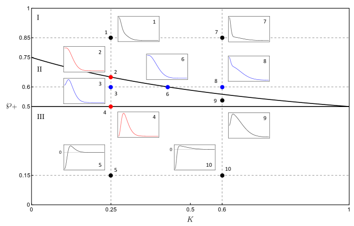
Figure 1: Behavior of $W(r)$ at ten different values of $(\text{\it\footnotesize K},\wp_{+})$, labeled from 1 to 10. Borderline cases are illustrated by points 2, 4, and 6. Note that point 6 is situated at $(0.43,0.6)$ (K value rounded to two decimal places), and point 9 is at $(0.6,0.53)$. All insets show $W(r)$ from zero and above in the region $\wp_{+}\geq 0.5$. For $W(r)$ in $\wp_{+}<0.5$ (i.e. points 5 and 10), $W=0$ is marked on the vertical axis in the insets. A Hopf bifurcation occurs when ${\rm I}\to{\rm II}$ along $\wp_{+}$ ($1\to 2\to 3$), while an inverse stochastic bifurcation occurs for ${\rm II}\to{\rm I}$ along K ($3\to 6\to 8$). A ${\rm II}\to{\rm III}$ crossover cannot happen without $W(0)$ becoming negative. We find for all K values that $W(0)$ is controlled by $\wp_{+}$ as illustrated in the sequence of changes along $\text{\it\footnotesize K}=0.25$ ($1\to 2\to 3\to 4\to 5$), or along $\text{\it\footnotesize K}=0.6$ ($7\to 8\to 9\to 10$). Phase III is “quantum protected” where the noise-induced oscillations are robust against thermal noise in retaining both its nonclassicality and limit-cycle behavior.

The Wigner function $\bar{W}_{\rm ss}(\alpha,\alpha^{*})$ in (16) cannot be negative without it being negative at the origin. To see this, we use the rotational symmetry of $W_{\text{ss}}(x,y)$ and consider $W_{\text{ss}}(x,0)$ for $x\geq 0$ without loss of generality. Suppose now $W_{\text{ss}}(x,0)$ contains negative values for some $x_{*}>0$, we then have

$$\frac{\wp_{+}-(1-\wp_{+})/\sqrt{\text{\it\footnotesize K}}}{1-\sqrt{\text{\it\footnotesize K}}}\,\exp\!\left(-\,\frac{\sqrt{\text{\it\footnotesize K}}}{1-\sqrt{\text{\it\footnotesize K}}}\;x_{*}^{2}\right)+\frac{\wp_{+}+(1-\wp_{+})/\sqrt{\text{\it\footnotesize K}}}{1+\sqrt{\text{\it\footnotesize K}}}\,\exp\!\left(\frac{\sqrt{\text{\it\footnotesize K}}}{1+\sqrt{\text{\it\footnotesize K}}}\;x_{*}^{2}\right)<0\;.$$ (41)

Upon rearranging gives

$$\exp\!\left(\frac{2\sqrt{\text{\it\footnotesize K}}}{1-\text{\it\footnotesize K}}\;x_{*}^{2}\right)<\frac{(1-\wp_{+})/\sqrt{\text{\it\footnotesize K}}-\wp_{+}}{1-\sqrt{\text{\it\footnotesize K}}}\bigg{[}\frac{1+\sqrt{\text{\it\footnotesize K}}}{\wp_{+}+(1-\wp_{+})/\sqrt{\text{\it\footnotesize K}}}\bigg{]}$$ (42)

for some $x_{*}>0$. Since the left-hand side is monotonically increasing in $x$, this condition must also be satisfied for all $0\leq x\leq x_{*}$. Hence $W(r)$ contains negative values if and only if $W(0)$ is negative. From this we obtain the condition for Wigner negativity to be

$$\wp_{+}<\frac{1}{2}\;.$$ (43)

Summarizing, we obtain three qualitatively distinct phases of solutions in the $(\text{\it\footnotesize K},\wp_{+})$ parameter space (see Fig. 1):

• Phase I: No limit cycle and no Wigner negativity.

• Phase II: Limit cycle with a positive Wigner function.

• Phase III: Limit cycle with a negative Wigner function.

II.2 Example: Coherent initial state

To illustrate the ideas developed in the previous section, let us consider a specific example of an initial coherent state $|{\alpha}\rangle$. The even and odd steady-state populations are

$$\wp_{+}=e^{-|\alpha|^{2}}\cosh|\alpha|^{2}\;,\quad\wp_{-}=e^{-|\alpha|^{2}}\sinh|\alpha|^{2}\;.$$ (44)

Applying the limit cycle condition to coherent states, we obtain

$$|\alpha|^{2}>\frac{1}{2}\ln\left[\frac{2(1+\text{\it\footnotesize K})}{1-\text{\it\footnotesize K}}\right]\;.$$ (45)

From this we learn that if we add an infinite amount of external noise to the system (i.e. $\text{\it\footnotesize K}\longrightarrow 1$), then the oscillator must also possess an infinite amount of energy (i.e. $|\alpha|^{2}$) if a limit cycle is to be induced.

Recall that for the Wigner function to exhibit negativity, we must have $\wp_{+}<1/2$. From Eq. (44), it can be easily seen that $\wp_{+}>1/2$. In other words, it is impossible to induce a negative Wigner function by initializing in any coherent state. This can actually be extended to any state with a positive Wigner function (including Gaussian states) as follows: If $\bar{W}(\alpha,\alpha^{*})>0$, then $\bar{W}(0,0)\propto(\wp_{+}-\wp_{-})>0$, which implies $\wp_{+}>1/2$. Since number parity is conserved, the Wigner function at the origin remains positive in the steady state. Moreover, the steady state Wigner function in (16) precludes any negativity without $\bar{W}(0,0)<0$, hence the entire Wigner function remains positive in the steady state. Note the converse is not true, i.e. a $\rho(0)$ with a negative Wigner function may have $\wp_{+}>1/2$. An example is the even cat state.

II.3 Tail behavior

At large distances from the origin, the steady-state Wigner function is asymptotic to the unnormalized Gaussian

$$W_{G}(x,y)=\frac{1-\sqrt{\text{\it\footnotesize K}}}{4\,\pi\sqrt{\text{\it\footnotesize K}}}\,\big{[}\,1-(1-\sqrt{\text{\it\footnotesize K}}\,)\,\wp_{+}\big{]}\,\exp\!\left[-\frac{1-\sqrt{\text{\it\footnotesize K}}}{2\,(1+\sqrt{\text{\it\footnotesize K}})}\,(x^{2}+y^{2})\right]\;.$$ (46)

Denoting the total area under $W_{G}(x,y)$ as $A$, we find that

$$\frac{1+\sqrt{\text{\it\footnotesize K}}}{2}\leq A=\frac{1+\sqrt{\text{\it\footnotesize K}}}{2\,\sqrt{\text{\it\footnotesize K}}}\,\big{[}1-(1-\sqrt{\text{\it\footnotesize K}}\,)\,\wp_{+}\big{]}\leq\frac{1+\sqrt{\text{\it\footnotesize K}}}{2\sqrt{\text{\it\footnotesize K}}}\;.$$ (47)

This shows that $A\longrightarrow 1$ as $\text{\it\footnotesize K}\longrightarrow 1$. This implies that the state becomes more Gaussian-like in the high-excitation limit, which is physically intuitive.

III Classical steady-state probability density

Here we solve for the steady-state probability density function for the classical system defined by the Itô stochastic differential equation,

$$d\alpha(t)=\big{[}\!-i\,\omega_{0}\,\alpha(t)+2\,\kappa\,\alpha(t)-\Delta\,|\alpha(t)|^{2}\,\alpha(t)\big{]}\,dt+\alpha^{*}(t)\,dW(t)\;.$$ (48)

where $\omega_{0}$ is the frequency of the free oscillations and $\Delta>0$. As in the main text, $dW(t)$ is a complex Wiener increment satisfying

$$dW^{*}(t)\,dW(t)=4\,\kappa\,dt\;.$$ (49)

III.1 Polar coordinates $(R,\Phi)$

A major simplification occurs if we convert from the complex-variable description to polar coordinates.

$$\alpha(t)=R(t)\,e^{i\Phi(t)}\;.$$ (50)

With the exception of $\alpha$, we denote random processes using capital letters and their realizations using the corresponding small letter. The stochastic dynamics of $R(t)$ and $\Phi(t)$ may then be derived using standard techniques Gar09 . They are given by

$$dR(t)={} \big{[}\,3\,\kappa\,R(t)-\Delta\,R^{3}(t)\big{]}dt+\frac{R(t)}{2}\,dW_{R}(t)\;,$$ (51)

$$d\Phi(t)={} -\omega_{0}\,dt+\frac{1}{2}\,dW_{\Phi}(t)\;,$$ (52)

where $dW_{R}(t)$ and $dW_{\Phi}(t)$ are independent real Wiener increments obeying the following Itô rules

$$dW_{R}(t)\,dW_{\Phi}(t)=0\;,$$ (53)

$$\big{[}dW_{R}(t)\big{]}^{2}=\big{[}dW_{\Phi}(t)\big{]}^{2}=8\,\kappa\,dt\;.$$ (54)

From (51) and (52) we can see that the dynamics of $R(t)$ and $\Phi(t)$ are independent processes and our two-dimensional system simplifies to two one-dimensional systems. This independence of $R(t)$ and $\Phi(t)$ means that each process has its own Fokker–Planck equation. For $R(t)$, it is given by

$$\frac{\partial}{\partial t}\;P_{R}(r,t)\equiv\mathscr{L}_{R}\,P_{R}(r,t)=-\frac{\partial}{\partial r}\big{(}3\,\kappa\,r-\Delta\,r^{3}\big{)}P_{R}(r,t)+\frac{1}{2}\,\frac{\partial^{2}}{\partial r^{2}}\,2\,\kappa\,r^{2}\,P_{R}(r,t)\;.$$ (55)

This permits a closed-form solution for the radial steady-state distribution,

$$\wp_{R}(r)\equiv\lim_{t\to\infty}P_{R}(r,t)=\frac{\Delta}{\kappa}\;r\,e^{-\Delta r^{2}/2\kappa}\;.$$ (56)

Note this has the form of a Rayleigh distribution. Similarly the phase dynamics in (52) corresponds to the operator $\mathscr{L}_{\Phi}$

$$\frac{\partial}{\partial t}\;P_{\Phi}(\phi,t)\equiv\mathscr{L}_{\Phi}\,P_{\Phi}(\phi,t)=-\frac{\partial}{\partial\phi}(-\omega_{0})P_{\Phi}(\phi,t)+\frac{1}{2}\,\frac{\partial^{2}}{\partial\phi^{2}}\,2\,\kappa\,P_{\Phi}(\phi,t)\;.$$ (57)

Imposing periodic boundary conditions (suitable for a circular variable such as $\Phi$) on a $2\pi$ interval gives

$$\wp_{\Phi}(\phi)\equiv\lim_{t\to\infty}P_{\Phi}(\phi,t)=\frac{1}{2\pi}\;.$$ (58)

Since the radial and phase motions are independent, we have $\tilde{P}(r,\phi,t)=P_{R}(r,t)P_{\Phi}(\phi,t)$ whose evolution can be obtained by adding the operators $\mathscr{L}_{R}$ and $\mathscr{L}_{\Phi}$,

$$\frac{\partial}{\partial t}\;\tilde{P}(r,\phi,t)\equiv\tilde{\mathscr{L}}\tilde{P}(r,\phi,t)=(\mathscr{L}_{R}+\mathscr{L}_{\Phi})\tilde{P}(r,\phi,t)\;.$$ (59)

The joint steady-state distribution for $R(t)$ and $\Phi(t)$ is therefore simply

$$\tilde{P}_{\rm ss}(r,\phi)\equiv{} \lim_{t\to\infty}\tilde{P}(r,\phi,t)$$ (60)

$$={} \wp_{R}(r)\,\wp_{\Phi}(\phi)=\frac{\Delta}{2\pi\kappa}\;r\,e^{-\Delta r^{2}/2\kappa}\;.$$ (61)

We have also numerically verified (61) by simulating the Itô stochastic differential equations (51) and (52). An example of the sampled distributions are shown in Fig. 2 (see figure caption for parameter values). Note from this result we can already see a qualitative difference between the classical and quantum systems. The classical steady-state distribution lacks the exponential growth present in $\tilde{W}_{\rm ss}(r,\phi)$. A well-known property of the Rayleigh distribution is that it is the probability density for the modulus of a complex random variable whose real and imaginary parts are independent and identically distributed Gaussians with zero mean. Thus, the form of (56) already tells us that $\alpha(t)$ is described by two independent processes in phase space.

Figure 2: Histograms from numerical simulations of (51) and (52) for $\kappa=\Delta=1$, $\omega_{0}=10$ with $10^{6}$ samples. Since we are only interested in the steady state, the transient dynamics in the stochastic simulations are discarded. (a) Radial probability density (ideally a Rayleigh distribution, shown by the orange line). (b) Phase probability density (ideally uniform on a $2\pi$ interval, orange line).

III.2 Cartesian coordinates $(X,Y)$

We can directly convert (61) to Cartesian coordinates. We define here $(X,Y)$ as earlier

$$X(t)=2R(t)\cos[\Phi(t)]\;,\quad Y(t)=2R(t)\sin[\Phi(t)]\;.$$ (62)

As with the Wigner function,

$$R(t)=\frac{1}{2}\sqrt{X^{2}(t)+Y^{2}(t)}\;,\quad\Phi(t)=\arctan\bigg{[}\frac{Y(t)}{X(t)}\bigg{]}\;,$$ (63)

and we obtain at once,

$$P_{\rm ss}(x,y)=\frac{1}{2\sqrt{x^{2}+y^{2}}}\;\tilde{P}_{\rm ss}(r(x,y),\phi(x,y))=\frac{\Delta}{8\pi\kappa}\;e^{-\Delta(x^{2}+y^{2})/8\kappa}\;,$$ (64)

We can verify that this is indeed the correct probability distribution in phase space by directly substituting this back into the Fokker–Planck equation for $X(t)$ and $Y(t)$. We define here

$$\alpha(t)=\frac{1}{2}\,[X(t)+i\,Y(t)]\;,$$ (65)

so that on taking the real and imaginary parts of (48) we get

$$dX(t)={} \bigg{\{}\omega_{0}\,Y(t)+2\,\kappa\,X(t)-\frac{\Delta}{4}\,\big{[}X^{2}(t)+Y^{2}(t)\big{]}X(t)\bigg{\}}\,dt+\frac{1}{2}\,\big{[}X(t)\,dW_{X}(t)+Y(t)\,dW_{Y}(t)\big{]}\;,$$ (66)

$$dY(t)={} \bigg{\{}\!-\omega_{0}\,X(t)+2\,\kappa\,Y(t)-\frac{\Delta}{4}\,\big{[}X^{2}(t)+Y^{2}(t)\big{]}Y(t)\bigg{\}}\,dt+\frac{1}{2}\,\big{[}X(t)\,dW_{Y}(t)-Y(t)\,dW_{X}(t)\big{]}\;.$$ (67)

The noise terms in (66) and (67) arise from decomposing $dW(t)$ into its real and imaginary parts in a similar fashion as $\alpha(t)$,

$$dW(t)=\frac{1}{2}\,\big{[}dW_{X}(t)+i\,dW_{Y}(t)\big{]}\;,$$ (68)

where $dW_{X}(t)$ and $dW_{Y}(t)$ are independent real Wiener increments

$$\big{[}dW_{X}(t)\big{]}^{2}=\big{[}dW_{Y}(t)\big{]}^{2}=8\,\kappa\,dt\;.$$ (69)

The Fokker–Planck equation corresponding to (66) and (67) is

$$\frac{\partial}{\partial t}\;P(x,y,t)\equiv\mathscr{L}\,P(x,y,t)={} -\frac{\partial}{\partial x}\bigg{[}\omega_{0}\,y+2\,\kappa\,x-\frac{\Delta}{4}\,(x^{2}+y^{2})x\bigg{]}P(x,y,t)+\frac{1}{2}\,\frac{\partial^{2}}{\partial x^{2}}\,2\,\kappa\,(x^{2}+y^{2})P(x,y,t)$$

$$-\frac{\partial}{\partial y}\bigg{[}-\omega_{0}\,x+2\,\kappa\,y-\frac{\Delta}{4}\,(x^{2}+y^{2})y\bigg{]}P(x,y,t)+\frac{1}{2}\,\frac{\partial^{2}}{\partial y^{2}}\,2\,\kappa\,(x^{2}+y^{2})P(x,y,t)\;.$$ (70)

We then find from (64) and (III.2) that

$$\mathscr{L}\,P_{\rm ss}(x,y)=0\;.$$ (71)

This is also numerically verified in Fig. 3 using (66) and (67) from which we see the sampled $P_{\text{ss}}(x,y)$ shows good agreement with the exact Gaussian distribution. It is worth pointing out here that we have also checked the consistency between the stochastic differential equations in polar coordinates against those in Cartesian coordinates by plotting $(X,Y)$ as $(2R\cos\Phi,2R\sin\Phi)$. The steady-state distribution for the latter is again a Gaussian as expected. It is generally useful to simulate stochastic differential equations as they provide some intuition for the processes of interest via direct visualization. Although we have not shown such results here, a good way to proceed is to use (51) and (52) instead of (66) and (67) as the former pair of equations are decoupled.

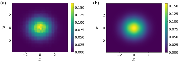
Figure 3: (a) Density plot for the Cartesian probability distribution $P_{\text{ss}}(x,y)$ generated from (66) and (67) for $\kappa=\Delta=1,\omega_{0}=10$ with $10^{6}$ samples. The transient dynamics is discarded. (b) Density plot for the analytical Gaussian distribution in (64).

IV Rotational flow in quantum phase space

IV.1 Definition

The goal here is to generalise the measure of circulation from Refs. TT74 ; TOT74 to an open quantum system. To motivate the generalisation to quantum mechanics we begin with a deterministic classical system defined by

$$\frac{d}{dt}\,x=f(x,y)\;,\quad\frac{d}{dt}\,y=g(x,y)\;.$$ (72)

If the phase-space point has circular motion then we can expect that it should have a nonvanishing angular momentum in phase space. It thus makes sense to define an angular momentum in phase space in analogous fashion to the orbital angular momentum of a mechanical point particle, except now the position and velocity vectors are given by their phase-space analogues. Using an orthonormal basis $\{{\bm{e}}_{x},{\bm{e}}_{y}\}$ in Cartesian coordinates, we may then define the phase-space position vector ${\bm{u}}=x\,{\bm{e}}_{x}+y\,{\bm{e}}_{y}$, and phase-space velocity vector ${\bm{v}}=f(x,y)\,{\bm{e}}_{x}+g(x,y)\,{\bm{e}}_{y}$. We then define the angular-momentum vector as the cross product,

$${\bm{u}}\times{\bm{v}}=[x\,g(x,y)-y\,f(x,y)]\,({\bm{e}}_{x}\times{\bm{e}}_{y})\;.$$ (73)

In fact, we will not be interested in ${\bm{u}}\times{\bm{v}}$ as a vector quantity, so we will simply define

$$\varphi\equiv\big{\|}{\bm{u}}\times{\bm{v}}\big{\|}=\big{|}x\,g(x,y)-y\,f(x,y)\big{|}\;.$$ (74)

If the system is noisy, so that $x(t)$ and $y(t)$ become random processes $X(t)$ and $Y(t)$, then an average over the realisations of $X(t)$ and $Y(t)$ may be performed as a sensible generalisation of (74),

$$\varphi\equiv{} \big{|}{\rm E}\big{[}X\,g(X,Y)-Y\,f(X,Y)\big{]}\big{|}\;,$$ (75)

where ${\rm E}[f(X,Y)]$ denotes a classical ensemble average of $f(X,Y)$ agains $P(x,y,t)$. Note that if we add multiplicative white noise to (72), then (75) assumes that $g(X,Y)$ and $f(X,Y)$ correspond to the Stratonovich forms of (72), either by directly interpreting (72) as Stratonovich equations or by finding the equivalent Stratonovich forms.

A further generalisation of $\varphi$ to quantum mechanics is then possible on letting $X\longrightarrow\hat{x}$ and $Y\longrightarrow\hat{y}$, except that upon quantization, $\hat{x}$ and $\hat{y}$ become canonically conjugate, satisfying

$$[\hat{x},\hat{y}]=2\,i\,\hat{1}\;.$$ (76)

However, quantization also entails that we choose a particular ordering between $\hat{x}$ and $\hat{y}$ in such a way that $\hat{x}$ and $\hat{y}$ remain Hermitian under time evolution. This results in the new functions $\breve{f}(\hat{x},\hat{y})$ and $\breve{g}(\hat{x},\hat{y})$ respectively. By the same token, we define $\varphi$ in quantum mechanics by the following symmetrized form

$$\varphi\equiv{} \frac{1}{2}\;\big{|}\big{\langle}\big{[}\hat{x}\,\breve{g}(\hat{x},\hat{y})+\breve{g}(\hat{x},\hat{y})\,\hat{x}\big{]}-\big{[}\hat{y}\,\breve{f}(\hat{x},\hat{y})+\breve{f}(\hat{x},\hat{y})\,\hat{y}\big{]}\big{\rangle}\big{|}\;.$$ (77)

This ensures that $\varphi$ is real valued, as it should be. If the system has a generator of time evolution given by ${\cal L}$, i.e. $d\rho(t)/dt={\cal L}\rho(t)$, then we replace $\breve{f}(\hat{x},\hat{y})$ and $\breve{g}(\hat{x},\hat{y})$ by using the adjoint of ${\cal L}$, defined with respect to the Hilbert–Schmidt inner product,

$${\rm Tr}\big{[}\hat{A}^{\dagger}{\cal L}^{\dagger}\hat{B}\big{]}={\rm Tr}\big{[}({\cal L}\hat{A})^{\dagger}\hat{B}\big{]}\;.$$ (78)

we therefore arrive at

$$\varphi\equiv{} \big{|}\,\Re\!\left[\left\langle\hat{x}\,{\cal L}^{\dagger}\hat{y}-\hat{y}\,{\cal L}^{\dagger}\hat{x}\right\rangle\right]\big{|}\;,$$ (79)

where $\Re[z]=(z+z^{*})/2$.

IV.2 General formula for the microscopic oscillator

Here we wish to derive $\varphi$ for the noise-induced oscillator defined by

$${\cal L}_{\Uparrow}=-i\,\omega_{0}\,[\hat{a}^{\dagger}\hat{a},\text{\Large$\cdot$}\,]+\kappa_{\Downarrow}{\cal D}[\hat{a}^{2}]+\kappa_{\Uparrow}{\cal D}[\hat{a}^{\dagger}{}^{2}]\;.$$ (80)

It is straightforward to show that

$${\cal L}_{\Uparrow}^{\dagger}=i\,\omega_{0}\,[\hat{a}^{\dagger}\hat{a},\text{\Large$\cdot$}]+\kappa_{\Downarrow}\,\big{(}{\cal D}[\hat{a}^{2}]\big{)}^{\dagger}+\kappa_{\Uparrow}\,\big{(}{\cal D}[\hat{a}^{\dagger}{}^{2}]\big{)}^{\dagger}\;,$$ (81)

where

$$\big{(}{\cal D}[\hat{a}^{2}]\big{)}^{\dagger}=\hat{a}^{\dagger}{}^{2}\,\text{\Large$\cdot$}\,\hat{a}{}^{2}-\frac{1}{2}\;\hat{a}^{\dagger}{}^{2}\,\hat{a}^{2}\,\text{\Large$\cdot$}-\frac{1}{2}\;\text{\Large$\cdot$}\,\hat{a}^{\dagger}{}^{2}\,\hat{a}^{2}\;,$$ (82)

$$\big{(}{\cal D}[\hat{a}^{\dagger}{}^{2}]\big{)}^{\dagger}=\hat{a}^{2}\,\text{\Large$\cdot$}\,\hat{a}^{\dagger}{}^{2}-\frac{1}{2}\;\hat{a}^{2}\,\hat{a}^{\dagger}{}^{2}\,\text{\Large$\cdot$}-\frac{1}{2}\;\text{\Large$\cdot$}\,\hat{a}^{2}\,\hat{a}^{\dagger}{}^{2}\;.$$ (83)

The expectation value in (79) becomes

$$\big{\langle}{\hat{x}\,{\cal L}^{\dagger}\hat{y}-\hat{y}\,{\cal L}^{\dagger}\hat{x}}\big{\rangle}={} i\,\omega_{0}\,\big{\langle}{\hat{x}\,[\hat{a}^{\dagger}\hat{a},\hat{y}]-\hat{y}\,[\hat{a}^{\dagger}\hat{a},\hat{x}]}\big{\rangle}+\kappa_{\Uparrow}\,\big{\langle}{\hat{x}\,\big{(}{\cal D}[\hat{a}^{\dagger}{}^{2}]\big{)}^{\dagger}\hat{y}-\hat{y}\,\big{(}{\cal D}[\hat{a}^{\dagger}{}^{2}]\big{)}^{\dagger}\hat{x}}\big{\rangle}$$

$$+\kappa_{\Downarrow}\,\big{\langle}{\hat{x}\,\big{(}{\cal D}[\hat{a}^{2}]\big{)}^{\dagger}\hat{y}-\hat{y}\,\big{(}{\cal D}[\hat{a}^{2}]\big{)}^{\dagger}\hat{x}}\big{\rangle}\;.$$ (84)

As we explained in the main text, an intuitive understanding of the dissipators in phase space suggests that they do not contribute to $\varphi$. This can be shown by writing $\hat{x}$ and $\hat{y}$ in terms of $\hat{a}$ and $\hat{a}^{\dagger}$. For the terms proportional to $\kappa_{\Uparrow}$ we have,

$$\big{\langle}{\hat{x}\,\big{(}{\cal D}[\hat{a}^{\dagger}{}^{2}]\big{)}^{\dagger}\hat{y}-\hat{y}\,\big{(}{\cal D}[\hat{a}^{\dagger}{}^{2}]\big{)}^{\dagger}\hat{x}}\big{\rangle}={} -i\,\big{\langle}{(\hat{a}+\hat{a}^{\dagger})\,\big{(}{\cal D}[\hat{a}^{\dagger}{}^{2}]\big{)}^{\dagger}(\hat{a}-\hat{a}^{\dagger})}\big{\rangle}+i\,\big{\langle}{(\hat{a}-\hat{a}^{\dagger})\,\big{(}{\cal D}[\hat{a}^{\dagger}{}^{2}]\big{)}^{\dagger}(\hat{a}+\hat{a}^{\dagger})}\big{\rangle}$$ (85)

$$={} i\,2\,\big{\langle}{\hat{a}\,\big{(}{\cal D}[\hat{a}^{\dagger}{}^{2}]\big{)}\!^{\dagger}\hat{a}^{\dagger}}\big{\rangle}-i\,2\,\big{\langle}{\hat{a}^{\dagger}\big{(}{\cal D}[\hat{a}^{\dagger}{}^{2}]\big{)}^{\dagger}\hat{a}}\big{\rangle}\;.$$ (86)

Similarly, the terms proportional to $\kappa_{\Downarrow}$ follow on replacing $\hat{a}^{\dagger}{}^{2}$ by $\hat{a}^{2}$ in the dissipator,

$$\big{\langle}{\hat{x}\,\big{(}{\cal D}[\hat{a}^{2}]\big{)}^{\dagger}\hat{y}-\hat{y}\,\big{(}{\cal D}[\hat{a}^{2}]\big{)}^{\dagger}\hat{x}}\big{\rangle}=i\,2\,\big{\langle}{\hat{a}\,\big{(}{\cal D}[\hat{a}^{2}]\big{)}^{\dagger}\hat{a}^{\dagger}}\big{\rangle}-i\,2\,\big{\langle}{\hat{a}^{\dagger}\big{(}{\cal D}[\hat{a}^{2}]\big{)}^{\dagger}\hat{a}}\big{\rangle}\;.$$ (87)

The expectation values in (86) and (87) now contain equal numbers of $\hat{a}$ and $\hat{a}^{\dagger}$ which means that ultimately they can be written in terms of the Hermitian operator $\hat{n}=\hat{a}^{\dagger}\hat{a}$. They are thus purely imaginary and vanish on substitution into the definition of $\varphi$ in (79). For the sake of concreteness we state their exact forms here,

$$\big{\langle}{\hat{x}\,\big{(}{\cal D}[\hat{a}^{\dagger}{}^{2}]\big{)}^{\dagger}\hat{y}-\hat{y}\,\big{(}{\cal D}[\hat{a}^{\dagger}{}^{2}]\big{)}^{\dagger}\hat{x}}\big{\rangle}={} i\,4\,(\langle{\hat{n}}\rangle+1)\;,$$ (88)

$$\big{\langle}{\hat{x}\,\big{(}{\cal D}[\hat{a}^{2}]\big{)}^{\dagger}\hat{y}-\hat{y}\,\big{(}{\cal D}[\hat{a}^{2}]\big{)}^{\dagger}\hat{x}}\big{\rangle}={} -i\,4\,\langle{\hat{n}}\rangle\;.$$ (89)

The expression for $\varphi$ therefore simplifies to

$$\varphi=\omega_{0}\,\big{\langle}{\hat{x}^{2}+\hat{y}^{2}}\big{\rangle}\;.$$ (90)

IV.3 Steady-state formula for the microscopic oscillator

We can now derive an explicit formula for the steady-state circulation by using our result for $\rho_{\rm ss}$. Since the steady state is diagonal in the number basis, it is more convenient to reexpress (90) as

$$\varphi=4\,\omega_{0}\bigg{(}\langle{\hat{n}}\rangle+\frac{1}{2}\bigg{)}\;.$$ (91)

Note the $1/2$ in the parentheses represents a vacuum contribution to the phase-space circulation. The steady-state average photon number is then, upon using (1),

$$\langle{\hat{n}}\rangle_{\rm ss}=2\,\big{(}1-\text{\it\footnotesize K}\big{)}\,\sum_{n=0}^{\infty}n\,\text{\it\footnotesize K}^{n}+2\,\wp_{-}\,\big{(}1-\text{\it\footnotesize K}\big{)}\,\sum_{n=0}^{\infty}\text{\it\footnotesize K}^{n}\;,$$ (92)

where we have used $\wp_{+}+\wp_{-}=1$. The second sum is simply a geometric series while it is simple to show that the first sum is given by

$$\sum_{n=0}^{\infty}\;n\,\text{\it\footnotesize K}^{n}=\frac{\text{\it\footnotesize K}}{(1-\text{\it\footnotesize K})^{2}}\;.$$ (93)

Equation (92) therefore becomes

$$\langle{\hat{n}}\rangle_{\rm ss}=\frac{2\,\text{\it\footnotesize K}}{1-\text{\it\footnotesize K}}+\wp_{-}\;.$$ (94)

Substituting this back into (91) we thus arrive at an expression for the steady-state circulation $\varphi_{\rm ss}$

$$\varphi_{\rm ss}=4\,\omega_{0}\,\bigg{(}\,\frac{2\,\text{\it\footnotesize K}}{1-\text{\it\footnotesize K}}+\wp_{-}+\frac{1}{2}\,\bigg{)}\;.$$ (95)

We may also express $\varphi_{\rm ss}$ as a function of only either $\wp_{0}$ or $\wp_{1}$, where $\wp_{n}=\langle{n}|\rho_{\rm ss}|{n}\rangle$. Choosing here to write it as a function of $\wp_{0}$ we note that $\wp_{-}$ may be written as

$$\wp_{-}=\frac{1-\text{\it\footnotesize K}-\wp_{0}}{1-\text{\it\footnotesize K}}\;,$$ (96)

where we have used (or see Refs. SL75 ; SL78 ),

$$\wp_{+}=\frac{\wp_{0}}{1-\text{\it\footnotesize K}}\;,\quad\wp_{-}=\frac{\wp_{1}}{1-\text{\it\footnotesize K}}\;.$$ (97)

Substituting (96) into (95) then gives

$$\varphi_{\rm ss}=4\,\omega_{0}\,\bigg{[}\frac{1+\text{\it\footnotesize K}-\wp_{0}}{1-\text{\it\footnotesize K}}+\frac{1}{2}\bigg{]}\;.$$ (98)

IV.4 Steady-state formula for the macroscopic oscillator

The definition of $\varphi$ for a classical system was already discussed en route to the quantum-mechanical definition in (75). Using the stochastic differential equations in (66) and (67) it is trivial to see that the time-dependent circulation is

$$\varphi=\omega_{0}\,{\rm E}\big{[}X^{2}(t)+Y^{2}(t)\big{]}\;.$$ (99)

The steady-state value then follows simply by noting that $X^{2}(t)+Y^{2}(t)=4R^{2}(t)$, and that the statistical moments for the Rayleigh distribution are well documented. For a Rayleigh distribution in the form of (56), the steady-state mean and variance are

$${\rm E}_{\rm ss}\big{[}R(t)\big{]}=\sqrt{\frac{\pi\kappa}{2\Delta}}\;,\quad{\rm V}_{\rm ss}\big{[}R(t)\big{]}={\rm E}_{\rm ss}\big{[}R^{2}(t)\big{]}-\big{\{}{\rm E}_{\rm ss}\big{[}R(t)\big{]}\big{\}}^{2}=\frac{(4-\pi)\kappa}{2\Delta}\;.$$ (100)

We thus have

$$\varphi_{\rm ss}=4\,\omega_{0}\,\Big{(}{\rm V}_{\rm ss}\big{[}R(t)\big{]}-\big{\{}{\rm E}_{\rm ss}\big{[}R(t)\big{]}\big{\}}^{2}\Big{)}=4\,\omega_{0}\,\bigg{(}\frac{2\,\kappa}{\Delta}\bigg{)}\;.$$ (101)

V Parity symmetry in the microscopic oscillator

Arguably no discussion of a conserved quantity can be considered complete without at least mentioning its associated symmetry. Thus we devote this section to some details and some further discussions related to the symmetry properties of our microscopic model in (80). For a symmetry operation represented by some unitary operator $\hat{U}$, we can distingush between two types of symmetries BP12 . We begin our discussion by recalling what they are from the literature. The first is called a strong symmetry. This requires that for a general Lindbladian

$${\cal L}=-\,i\,[\hat{H},\text{\Large$\cdot$}\,]+\sum_{k=1}^{M}\,\gamma_{k}\,{\cal D}[\hat{c}_{k}]\;,\quad\gamma_{k}\geq 0\,,\;\forall\;k\;,$$ (102)

$\hat{U}$ satisfies

$$[\,\hat{U},\hat{H}]=[\,\hat{U},\hat{c}_{k}]=0\;,\quad\forall\;k\;.$$ (103)

This can be understood to generalize the symmetry condition for Hamiltonian systems [defined by (102) with $\gamma_{k}=0$ for all values of $k$] to the case when dissipative processes are present. Of course, ${\cal L}$ is a generator of time evolution for a Markovian quantum system just as $\hat{H}$ is for a closed system. It thus also makes sense to define symmetry for an open system by requiring that the action of $\hat{U}$ commute with the Lindbladian, i.e.

$$[\,{\cal U},{\cal L}\,]=0\;.$$ (104)

where ${\cal U}$ is defined by ${\cal U}\,\rho=\hat{U}\,\rho\,\hat{U}^{-1}$. If we find a $\hat{U}$ that satisfies (104), it is said to be a weak symmetry. Strong symmetry implies weak symmetry but not vice versa BP12 ; AJ14 .

Using the above, we can show that ${\cal L}_{\Uparrow}$ possesses a strong symmetry corresponding to photon-number parity, defined by $\hat{\Pi}=(-1)^{\hat{n}}$ where $\hat{n}=\hat{a}^{\dagger}\hat{a}$. It is simple to see that $\hat{\Pi}=\hat{\Pi}^{\dagger}=\hat{\Pi}^{-1}$. Since $\hat{\Pi}$ is a function the number operator it commutes with the Hamiltonian in (80). The only nontrivial requirements are from (103) with $\hat{c}_{1}=\hat{a}^{2}$ and $\hat{c}_{2}=\hat{a}^{\dagger}{}^{2}$,

$$[\hat{\Pi},\hat{a}^{2}]=[\hat{\Pi},\hat{a}^{\dagger}{}^{2}]=0\;.$$ (105)

This is simple to show and has been discussed in the context of two-photon absorption (i.e. $\kappa_{\Uparrow}=0$) AJ14 . As noted in the main text, parity conservation and strong symmetry are equivalent AJ14 . For a general ${\cal L}$, conservation of an arbitrary quantity represented by $\hat{C}$ is defined formally as

$${\cal L}^{\dagger}\hat{C}=0\;.$$ (106)

We may thus use the condition of strong symmetry to show that ${\cal L}_{\uparrow}$ does not conserve photon-number parity. We recall for convenience here that ${\cal L}_{\uparrow}$ is given by

$${\cal L}_{\uparrow}=-\,i\,\omega_{0}\,[\hat{a}^{\dagger}\hat{a},\text{\Large$\cdot$}\,]+\kappa_{\Downarrow}\,{\cal D}[\hat{a}^{2}]+\kappa_{\uparrow}\,{\cal D}[\hat{a}^{\dagger}]\;.$$ (107)

This is already intuitive from the appearance of ${\cal D}[\hat{a}^{\dagger}]$ in ${\cal L}_{\uparrow}$, since one-photon transitions take odd-parity number states to even-parity ones and vice versa. The corresponding mathematical statement is simply $[\hat{\Pi},\hat{a}^{\dagger}]=-2\,\hat{a}^{\dagger}\,\hat{\Pi}\neq 0$. The possibility of ${\cal L}_{\uparrow}$ to satisfying weak number-parity symmetry remains open. However, instead of showing this directly, here we point out that both ${\cal L}_{\uparrow}$ and ${\cal L}_{\Uparrow}$ satisfy continuous rotational symmetry for which parity symmetry is a special case of. A continuous rotation has the unitary operator $\hat{P}_{\phi}=\exp(-i\phi\,\hat{n})$ where $\phi$ is a continuous real-valued parameter. It is not difficult to show that the operation of a rotation in phase space commutes with either ${\cal L}_{\uparrow}$ and ${\cal L}_{\Uparrow}$,

$$[{\cal P}_{\phi},{\cal L}_{\uparrow}]=[{\cal P}_{\phi},{\cal L}_{\Uparrow}]=0\;.$$ (108)

where ${\cal P}_{\phi}\,\rho=\hat{P}_{\phi}\,\rho\,\hat{P}^{-1}_{\phi}$. This property was in fact shown in Ref. CHN+20 for ${\cal L}_{\Uparrow}$ but was referred to as phase covariance. Clearly photon-number parity transformation corresponds to a rotation with $\phi=\pi$. Thus, both ${\cal L}_{\uparrow}$ and ${\cal L}_{\Uparrow}$ exhibit a weak continuous symmetry defined by $\hat{P}_{\phi}$, and consequently a weak discrete symmetry given by $\hat{P}_{\pi}=\hat{\Pi}$ (noting of course that ${\cal L}_{\Uparrow}$ actually exhibits a strong symmetry as well).

Note that we have expressed $\rho_{\rm ss}$ in (1) deliberately as a linear combination of a state with even parity $\rho_{+}$, and a state with odd parity $\rho_{-}$. This is a very natural decomposition of $\rho_{\rm ss}$ given that photon-number parity is conserved. Its form makes the steady state simple to see if the initial state does not contain either even or odd number states. The normalization of $\rho_{\rm ss}$ is also trivial to see in when expressed in the form of (1). There is a closely related idea, in fact a theorem, which decomposes $\rho_{\rm ss}$ not in terms of states like (1), but in terms of an orthonormal operator basis. The expansion coefficients in this decomposition are defined by averages of conserved quantities with respect to the initial state AJ14 . We complete our discussion of the symmetry and conservation of parity by simply finding this an expansion for $\rho_{\rm ss}$. Given an initial state $\rho(0)$, and an ${\cal L}$ with no purely imaginary eigenvalues, Ref. AJ14 has shown that the steady state may be expanded in terms of $D$ linearly independent conserved quantities $\{\hat{C}_{k}\}_{k=0}^{D-1}$ in the following form

$$\rho_{\rm ss}=\sum_{k=0}^{D-1}\,{\rm Tr}\big{[}\hat{C}^{\dagger}_{k}\,\rho(0)\big{]}\,\hat{M}_{k}\;,$$ (109)

where $\{\hat{M}_{k}\}_{k=0}^{D-1}$ is an orthonormal basis with respect to the Hilbert–Schmidt inner product, i.e. ${\rm Tr}[\hat{M}^{\dagger}_{j}\hat{M}_{k}]=\delta_{j,k}$ .

To show that $\rho_{\rm ss}$ for ${\cal L}_{\Uparrow}$ can be put in the form of (109), we note that it has two linearly independent conserved quantities, namely the parity of even and odd photon numbers. Hence $D=2$. The expansion in (109) may then be achieved with

$$\hat{C}_{0}=\frac{\sqrt{1-\text{\it\footnotesize K}}}{2}\,\big{(}\hat{1}+\hat{\Pi}\big{)}\;,\quad\hat{C}_{1}=\frac{\sqrt{1-\text{\it\footnotesize K}}}{2}\,\big{(}\hat{1}-\hat{\Pi}\big{)}\;.$$ (110)

These operators are orthogonal since they contain only nonoverlapping projectors in the Fock basis. Orthogonality then implies linear independence. To see that they are conserved we note that ${\cal L}_{\Uparrow}^{\dagger}\,\hat{\Pi}={\cal L}_{\Uparrow}^{\dagger}\,\hat{1}=0$. These can be shown straightforwardly from (81)–(82). It then follows from the linearity of ${\cal L}_{\Uparrow}^{\dagger}$ that ${\cal L}_{\Uparrow}^{\dagger}\,\hat{C}_{0}={\cal L}_{\Uparrow}^{\dagger}\,\hat{C}_{1}=0$. The associated operator basis is then

$$\hat{M}_{0}=\sqrt{1-\text{\it\footnotesize K}}\,\sum_{n=0}^{\infty}\,\text{\it\footnotesize K}^{n}\,\left|{2n}\rangle\langle{2n}\right|\;,\quad\hat{M}_{1}=\sqrt{1-\text{\it\footnotesize K}}\,\sum_{n=0}^{\infty}\,\text{\it\footnotesize K}^{n}\,\left|{2n+1}\rangle\langle{2n+1}\right|\;.$$ (111)

Clearly $\hat{M}_{0}$ and $\hat{M}_{1}$ are clearly orthogonal to each other,

$${\rm Tr}\big{[}\hat{M}^{\dagger}_{0}\hat{M}_{1}\big{]}={} {\rm Tr}\big{[}\hat{M}^{\dagger}_{1}\hat{M}_{0}\big{]}=0\;.$$ (112)

It is also straightforward to see that they are normalized,

$${\rm Tr}\big{[}\hat{M}^{\dagger}_{0}\hat{M}_{0}\big{]}={\rm Tr}\big{[}\hat{M}^{\dagger}_{1}\hat{M}_{1}\big{]}=1\;.$$ (113)

One may also verify that the steady state written in the form of (109) using (110) and (111) is indeed normalized. Note that $\hat{M}_{0}$ and $\hat{M}_{1}$ are positive and Hermitian operators but do not have unit trace. We mention also that (109) applies in the case of $\kappa_{\Uparrow}=\text{\it\footnotesize K}=0$ as well. However, in this case there is an additional conserved quantity arising from the coherences as discussed in the main text, so that $D=3$. As we will not be using this, the reader is referred to Ref. AJ14 for the exact expression for the conserved quantity.

VI Classical detailed balance

VI.1 Definition

Let us now use the classical model to build some intuition about detailed balance and the nature of the probability current. A classical stochastic system with two degrees of freedom is said to possess detailed balance if the following relation is satisfied at steady state,

$$P_{\rm ss}(x_{2},y_{2},t+\tau\,;\,x_{1},y_{1},t)=P_{\rm ss}({\sf T}[x_{1}],{\sf T}[y_{1}],t+\tau\,;\,{\sf T}[x_{2}],{\sf T}[y_{2}],t)\;.$$ (114)

Here we are defining ${\sf T}[x]=\pi_{X}x$ and ${\sf T}[y]=\pi_{Y}y$ (also valid on replacing $x$ by $X$ and $y$ by $Y$), and $\pi_{X}$, $\pi_{Y}$ may be $\pm 1$ depending on whether $X$ and $Y$ are even ($+1$) or odd ($-1$) variables under time reversal. It can then be shown that a classical Markovian system given by $\partial P(x,y,t)/\partial t=\mathscr{L}P(x,y,t)$ satisfies detailed balance if and only if GH71 ; Ris72

$$P_{\rm ss}(x,y)=P_{\rm ss}({\sf T}[x],{\sf T}[y])\;,$$ (115)

where ${\sf T}$ denotes the operation of time reversal and

$$P_{\rm ss}(x,y)\,\mathscr{L}^{\dagger}(x,y)=\mathscr{L}({\sf T}[x],{\sf T}[y])\,P_{\rm ss}(x,y)\;.$$ (116)

We have also written out the dependence of $\mathscr{L}$ on $x$ and $y$ explicitly in order to define its time-reversed version. For real functions on $\mathbbm{R}^{2}$, the adjoint of $\mathscr{L}$ is defined by the inner product

$$\int^{\infty}_{-\infty}dx\int^{\infty}_{-\infty}dy\;f(x,y)\,\mathscr{L}^{\dagger}g(x,y)=\int^{\infty}_{-\infty}dx\int^{\infty}_{-\infty}dy\;g(x,y)\,\mathscr{L}f(x,y)\,\;.$$ (117)

For our macroscopic oscillator, $\mathscr{L}$ is defined by a Fokker–Planck equation in terms of drift vector ${\bm{A}}$, and a diffusion matrix $D$,

$$\bm{A}(x,y)=\left[\begin{array}[]{c}{A_{X}(x,y)}\\ {A_{Y}(x,y)}\end{array}\right]\;,\quad D(x,y)=\left[\begin{array}[]{cc}{D_{X}(x,y)}&{D_{XY}(x,y)}\\ {D_{Y\!X}(x,y)}&{D_{Y}(x,y)}\end{array}\right]\;.$$ (122)

These can be read off from (III.2), but for the purpose of this section, we work with the general form of $\mathscr{L}$, given by

$$\mathscr{L}=-\frac{\partial}{\partial x}A_{X}(x,y)-\frac{\partial}{\partial y}A_{Y}(x,y)+\frac{1}{2}\;\bigg{[}\frac{\partial^{2}}{\partial x^{2}}D_{X}(x,y)+2\,\frac{\partial^{2}}{\partial x\,\partial y}D_{XY}(x,y)+\frac{\partial^{2}}{\partial y^{2}}D_{Y}(x,y)\bigg{]}\;.$$ (123)

Note the diffusion matrix is always symmetric so that $D_{XY}(x,y)=D_{Y\!X}(x,y)$. Proving (115) and (116) to be true using (123) would not add any insight to our understanding of the microscopic oscillator. For us, the significance of (115) and (116) is that they have counterparts in quantum theory, as will be seen later. In the classical theory, they are also the necessary and sufficient conditions for the the steady-state probability current to be purely reversible GH71 ; Ris72 . In fact, conditions (115) and (116) for a general Markov process are satisfied if and only if at steady state, the probability flux is reversible and divergenceless, while the diffusion matrix transforms under time reversal as

$$D_{X}(x,y)=\pi^{2}_{X}\,D_{X}({\sf T}[x],{\sf T}[y])\;,\quad D_{Y}({\bm{z}})=\pi^{2}_{Y}\,D_{Y}({\sf T}[x],{\sf T}[y])\;,$$ (124)

$$D_{XY}(x,y)=\pi_{X}\,\pi_{Y}\,D_{XY}({\sf T}[x],{\sf T}[y])\;.$$ (125)

The separation of the probability current into reversible and irreversible components follow from a formal decomposition of the drift into reversible and irreversible parts. These depend on the time reversal properties of the drift vector, which are defined by

$$\stackrel{{\scriptstyle\;\text{\tiny$\leftrightarrow$}}}{{{\bm{A}}}}\!(x,y)=\frac{1}{2}\,\big{[}{\bm{A}}(x,y)-\Pi\,{\bm{A}}({\sf T}[x],{\sf T}[y])\big{]}\;,\quad\stackrel{{\scriptstyle\;\text{\tiny$\rightarrow$}}}{{{\bm{A}}}}\!(x,y)=\frac{1}{2}\,\big{[}{\bm{A}}(x,y)+\Pi\,{\bm{A}}({\sf T}[x],{\sf T}[y])\big{]}\;.$$ (126)

We have labelled the reversible drift using a bidirectional arrow and the irreversible drift by a unidirectional arrow. The matrix $\Pi$ is simply,

$$\Pi=\left[\begin{array}[]{cc}{\pi_{X}}&{0}\\ {0}&{\pi_{Y}}\end{array}\right]\;.$$ (129)

The probability current, which we denote by ${\bm{J}}$, is defined by writing the Fokker–Planck equation as a continuity equation for the probability density,

$$\frac{\partial}{\partial t}\;P(x,y,t)=-\nabla\,\text{\large$\cdot$}\,\bm{J}(x,y,t)\;.$$ (130)

We may then decompose the probability current by using (126) into reversible and irreversible parts,

$$\bm{J}(x,y,t)=\,\stackrel{{\scriptstyle\;\text{\tiny$\leftrightarrow$}}}{{\bm{J}}}\!\!(x,y,t)\;+\stackrel{{\scriptstyle\;\text{\tiny$\rightarrow$}}}{{\bm{J}}}\!\!(x,y,t)\;.$$ (131)

They are simply

$$\stackrel{{\scriptstyle\;\text{\tiny$\leftrightarrow$}}}{{\bm{J}}}\!\!(x,y,t)=\,\stackrel{{\scriptstyle\;\text{\tiny$\leftrightarrow$}}}{{{\bm{A}}}}\!(x,y)\,P(x,y,t)\;,\quad\stackrel{{\scriptstyle\;\text{\tiny$\rightarrow$}}}{{\bm{J}}}\!\!(x,y,t)=\,\stackrel{{\scriptstyle\;\text{\tiny$\rightarrow$}}}{{{\bm{A}}}}\!(x,y)\,P(x,y,t)-\frac{1}{2}\big{[}\nabla^{\top}D(x,y)P(x,y,t)\big{]}^{\top}\;,$$ (132)

where $S^{\top}$ denotes the matrix transpose of $S$. As is usual, the steady-state current may be formally defined as

$$\bm{j}(x,y)=\lim_{t\to\infty}\bm{J}(x,y,t)\;.$$ (133)

The condition for the steady-state probability current to be reversible and divergenceless can then be stated as

$$\nabla\,\text{\large$\cdot$}\!\stackrel{{\scriptstyle\;\text{\tiny$\leftrightarrow$}}}{{\bm{j}}}\!\!(x,y)=0\;,\quad\stackrel{{\scriptstyle\;\text{\tiny$\rightarrow$}}}{{\bm{j}}}\!\!(x,y)=\bm{0}\;.$$ (134)

We may simply use (132) and replace the time-dependent probability density by its steady-state value. As mentioned earlier, condition (134) along with (124) and (124) are equivalent to (115) and (116).

VI.2 Detailed balance in the macroscopic oscillator

The task of showing that our macroscopic oscillator satisfies (124), (125), and (134) is now a simple matter. Since we are thinking of the macroscopic variables $X$ and $Y$ as the classical limits of $\hat{x}$ and $\hat{y}$, these would have to be defined as even and odd variables under time reversal to be consistent with quantum mechanics SN21 . Hence,

$$\pi_{X}=1\;,\quad\pi_{Y}=-1\;.$$ (135)

The drift vector and diffusion matrix from (III.2) are

$$\bm{A}(x,y)=\left[\begin{array}[]{c}{\omega_{0}\,y+2\,\kappa\,x-\Delta\,(x^{2}+y^{2})x/4}\\ {-\omega_{0}\,x+2\,\kappa\,y-\Delta\,(x^{2}+y^{2})y/4}\end{array}\right]\;,\quad D(x,y)=\left[\begin{array}[]{cc}{2\kappa(x^{2}+y^{2})}&{0}\\ {0}&{2\kappa(x^{2}+y^{2})}\end{array}\right]\;.$$ (140)

Clearly, $D(x,y)$ satisfies (124) and (125). Recall that we have also shown in (64) the steady-state distribution of the macroscopic oscillator to be

$$P_{\rm ss}(x,y)=\frac{\Delta}{8\pi\kappa}\;e^{-\Delta(x^{2}+y^{2})/8\kappa}\;.$$ (141)

From these one find (134) to be true, and in particular, with

$$\stackrel{{\scriptstyle\;\text{\tiny$\leftrightarrow$}}}{{\bm{j}}}\!\!(x,y)=\left[\begin{array}[]{c}{\omega_{0}\,y}\\ {-\omega_{0}\,x}\end{array}\right]P_{\rm ss}(x,y)\;.$$ (144)

VII Quantum detailed balance

VII.1 Definition

A Markovian quantum system defined by $d\rho(t)/dt={\cal L}\,\rho(t)$ is said to be in detailed balance if and only if Aga73 ; CW76 ,

$$\big{\langle}{\hat{A}(t+\tau)\,\hat{B}(t)}\big{\rangle}_{\rm ss}=\big{\langle}{{\sf T}\big{[}\hat{B}(t+\tau)\big{]}\,{\sf T}\big{[}\hat{A}(t)\big{]}}\big{\rangle}_{\rm ss}\;,\quad\forall\;\hat{A},\hat{B}$$ (145)

where ${\sf T}$ denotes the operation of time reversal via an antiunitary and antilinear operator $\hat{T}$ SN21 . It maps operators to operators,

$${\sf T}(\hat{A})=\hat{T}\hat{A}^{\dagger}\,\hat{T}^{-1}\;,\quad\forall\;\hat{A}\;,$$ (146)

and scalars to their complex conjugates, i.e. $\hat{T}\,z\,\hat{T}^{-1}=z^{*}$ for $z\in\mathbbm{C}$. This condition of quantum detailed balance was first proposed in Ref. Aga73 , and rigorously justified in Ref. CW76 . It is more general than detailed balance in the sense of a Pauli equation. The latter is a semiclassical condition and is implied by (145). It can then be shown that if the steady state is time-reversal invariant, i.e.

$$\rho_{\rm ss}={\sf T}(\rho_{\rm ss})\;,$$ (147)

then (145) is implied by the following superoperator condition

$$\rho_{\rm ss}\,{\cal L}^{\dagger}={\sf T}({\cal L})\,\rho_{\rm ss}\;.$$ (148)

The time-reversed Lindbladian ${\sf T}({\cal L})$ is another superoperator defined such that,

$${\sf T}({\cal L}\hat{A})={\sf T}({\cal L})\,{\sf T}(\hat{A})\;,\quad\forall\;\hat{A}\;.$$ (149)

Thus if both (147) and (148) are true for a given ${\cal L}$ then quantum detailed balance is proven. Conditions (147) and (148) are analogs of (115) and (116), which is why we are using (145) to prove quantum detailed balance. But note that unlike (115) and (116) in the classical theory, (147) and (148) are only sufficient conditions for quantum detailed balance. For the microscopic oscillator given by ${\cal L}_{\Uparrow}$, the steady state is diagonal in the number basis, and since number states are time-reversal invariant, it follows that (147) holds. We thus only need to check (148) which requires the time-reversed Lindbladian.

VII.2 Time-reversed Lindbladian

Here we derive the time-reversed Lindbladian for the microscopic oscillator of ${\cal L}_{\Uparrow}$. Recall for convenience that ${\cal L}_{\Uparrow}$ is given by

$${\cal L}_{\Uparrow}=-i\,\omega_{0}\,[\hat{a}^{\dagger}\hat{a},\text{\Large$\cdot$}\,]+\kappa_{\Downarrow}\,\bigg{(}\hat{a}^{2}\,\text{\Large$\cdot$}\,\hat{a}^{\dagger}{}^{2}-\frac{1}{2}\,\hat{a}^{\dagger}{}^{2}\,\hat{a}^{2}\,\text{\Large$\cdot$}-\frac{1}{2}\,\text{\Large$\cdot$}\,\hat{a}^{\dagger}{}^{2}\hat{a}^{2}\bigg{)}+\kappa_{\Uparrow}\,\bigg{(}\hat{a}^{\dagger}{}^{2}\,\text{\Large$\cdot$}\,\hat{a}^{2}-\frac{1}{2}\,\hat{a}^{2}\,\hat{a}^{\dagger}{}^{2}\,\text{\Large$\cdot$}-\frac{1}{2}\,\text{\Large$\cdot$}\,\hat{a}^{2}\hat{a}^{\dagger}{}^{2}\bigg{)}\;.$$ (150)

Using (146), we therefore have for an arbitrary $\hat{A}$,

$${\sf T}({\cal L}_{\Uparrow}\hat{A})={} -i\,\omega_{0}\,\big{[}{\sf T}(\hat{A})\,{\sf T}(\hat{a})\,{\sf T}(\hat{a}^{\dagger})-{\sf T}(\hat{a})\,{\sf T}(\hat{a}^{\dagger})\,{\sf T}(\hat{A})\big{]}$$

$$+\kappa_{\Downarrow}\,\bigg{[}{\sf T}(\hat{a}^{\dagger}{}^{2})\,{\sf T}(\hat{A})\,{\sf T}(\hat{a}^{2})-\frac{1}{2}\,{\sf T}(\hat{A})\,{\sf T}(\hat{a}^{2})\,{\sf T}(\hat{a}^{\dagger}{}^{2})-\frac{1}{2}\,{\sf T}(\hat{a}^{2})\,{\sf T}(\hat{a}^{\dagger}{}^{2})\,{\sf T}(\hat{A})\bigg{]}$$

$$+\kappa_{\Uparrow}\,\bigg{[}{\sf T}(\hat{a}^{2})\,{\sf T}(\hat{A})\,{\sf T}(\hat{a}^{\dagger}{}^{2})-\frac{1}{2}\,{\sf T}(\hat{A})\,{\sf T}(\hat{a}^{\dagger}{}^{2})\,{\sf T}(\hat{a}^{2})-\frac{1}{2}\,{\sf T}(\hat{a}^{\dagger}{}^{2})\,{\sf T}(\hat{a}^{2})\,{\sf T}(\hat{A})\bigg{]}\;.$$ (151)

To work out ${\sf T}(\hat{a})$ and ${\sf T}(\hat{a}^{\dagger})$ we can write $\hat{a}=(\hat{x}+i\hat{y})/2$ and use the fact that $[\hat{x},\hat{y}]=i\,2\,\hat{1}$ enforces $\hat{x}$ to be an even operator, and $\hat{y}$ an odd operator under time reversal SN21 :

$${\sf T}(\hat{x})=\hat{x}\;,\quad{\sf T}(\hat{y})=-\hat{y}\;.$$ (152)

Using (152), the time-reversed annihilation and creation operators are then

$${\sf T}(\hat{a})=\frac{1}{2}\,\big{[}{\sf T}(\hat{x})-i\,{\sf T}(\hat{y})\big{]}=\hat{a}^{\dagger}\;,\quad{\sf T}(\hat{a}^{\dagger})=\frac{1}{2}\,\big{[}{\sf T}(\hat{x})+i\,{\sf T}(\hat{y})\big{]}=\hat{a}\;.$$ (153)

We may then simplify (VII.2) further since

$${\sf T}(\hat{a}^{2})={\sf T}(\hat{a}){\sf T}(\hat{a})=\hat{a}^{\dagger}{}^{2}\;,\quad{\sf T}(\hat{a}^{\dagger}{}^{2})={\sf T}(\hat{a}^{\dagger}){\sf T}(\hat{a}^{\dagger})=\hat{a}^{2}\;.$$ (154)

Using (149) we arrive at

$${\sf T}({\cal L}_{\Uparrow})\,{\sf T}(\hat{A})={} -i\,\omega_{0}\,\big{[}{\sf T}(\hat{A}),\hat{a}^{\dagger}\hat{a}\big{]}+\kappa_{\Downarrow}\,{\cal D}\big{[}\hat{a}^{2}\big{]}{\sf T}(\hat{A})+\kappa_{\Uparrow}\,{\cal D}\big{[}\hat{a}^{\dagger}{}^{2}\big{]}{\sf T}(\hat{A})\;.$$ (155)

Note that ${\sf T}({\cal L}_{\Uparrow})$ is not a time-reversed Lindbladian in the sense that it captures time-reversed motion of the microscopic oscillator, which is what time-reversal means in physics. In phase space, the time-reversed motion of ${\cal L}_{\Uparrow}$ should interachange motion in the positive $x$ direction with motion in the negative $x$ direction, and similarly for $y$. Thus time-reversed motion should interchange amplification with dissipation, and counterclockwise rotation with clockwise rotation. Although ${\sf T}({\cal L}_{\Uparrow})$ as defined by (149) does not correspond to time-reversal in this sense, it is nevertheless what is required mathematically by quantum detailed balance.

VII.3 Detailed balance in the microscopic oscillator

We are now in position to prove quantum detailed balance by using (148). Recall also from (81)–(82) that

$${\cal L}^{\dagger}=i\,\omega_{0}\,[\hat{a}^{\dagger}\hat{a},\text{\Large$\cdot$}\,]+\kappa_{\Uparrow}\,\bigg{(}\hat{a}^{2}\,\text{\Large$\cdot$}\,\hat{a}^{\dagger}{}^{2}-\frac{1}{2}\;\hat{a}^{2}\,\hat{a}^{\dagger}{}^{2}\,\text{\Large$\cdot$}-\frac{1}{2}\;\text{\Large$\cdot$}\,\hat{a}^{2}\,\hat{a}^{\dagger}{}^{2}\bigg{)}+\kappa_{\Downarrow}\,\bigg{(}\hat{a}^{\dagger}{}^{2}\,\text{\Large$\cdot$}\,\hat{a}{}^{2}-\frac{1}{2}\;\hat{a}^{\dagger}{}^{2}\,\hat{a}^{2}\,\text{\Large$\cdot$}-\frac{1}{2}\;\text{\Large$\cdot$}\,\hat{a}^{\dagger}{}^{2}\,\hat{a}^{2}\bigg{)}\;.$$ (156)

Equation (148) can then be written as, using (155) and (156),

$$\rho_{\rm ss}\,{\cal L}^{\dagger}-{\sf T}({\cal L})\rho_{\rm ss}={} i\,\omega_{0}\,[\rho_{\rm ss},\hat{a}^{\dagger}\hat{a}]\,\text{\Large$\cdot$}+\frac{1}{2}\,\kappa_{\Uparrow}\,[\hat{a}^{2}\hat{a}^{\dagger}{}^{2},\rho_{\rm ss}]\,\text{\Large$\cdot$}+\frac{1}{2}\,\kappa_{\Downarrow}\,[\hat{a}^{\dagger}{}^{2}\hat{a}^{2},\rho_{\rm ss}]\,\text{\Large$\cdot$}$$

$$+\big{(}\kappa_{\Uparrow}\,\rho_{\rm ss}\,\hat{a}^{2}-\kappa_{\Downarrow}\,\hat{a}^{2}\rho_{\rm ss}\big{)}\,\text{\Large$\cdot$}\,\hat{a}^{\dagger}{}^{2}+\big{(}\kappa_{\Downarrow}\,\rho_{\rm ss}\,\hat{a}^{\dagger}{}^{2}-\kappa_{\Uparrow}\,\hat{a}^{\dagger}{}^{2}\rho_{\rm ss}\big{)}\,\text{\Large$\cdot$}\,\hat{a}^{2}\;.$$ (157)

Note that since $\rho_{\rm ss}$ is diagonal in the number basis, it must commute with $\hat{n}=\hat{a}^{\dagger}\hat{a}$. Now since $\hat{a}^{2}\hat{a}^{\dagger}{}^{2}$ and $\hat{a}^{\dagger}{}^{2}\hat{a}^{2}$ may also be written in terms of $\hat{n}$, all commutator terms in (VII.3) vanish,

$$[\hat{a}^{\dagger}\hat{a},\rho_{\rm ss}]=[\hat{a}^{2}\hat{a}^{\dagger}{}^{2},\rho_{\rm ss}]=[\hat{a}^{\dagger}{}^{2}\hat{a}^{2},\rho_{\rm ss}]=0\;.$$ (158)

It therefore remains to show that the second line of (VII.3) vanishes. Using $\rho_{\rm ss}=\wp_{+}\rho_{+}+\wp_{-}\rho_{-}$ [recall (1)–(3)], we have

$$\kappa_{\Downarrow}\,\hat{a}^{2}\rho_{\rm ss}={} \wp_{+}\bigg{(}1-\frac{\kappa_{\Uparrow}}{\kappa_{\Downarrow}}\bigg{)}\sum_{n=1}^{\infty}\,\frac{\kappa_{\Uparrow}^{n}}{\kappa_{\Downarrow}^{n-1}}\,\sqrt{(2n)(2n-1)}\left|{2n-2}\rangle\langle{2n}\right|$$

$$+\wp_{-}\bigg{(}1-\frac{\kappa_{\Uparrow}}{\kappa_{\Downarrow}}\bigg{)}\sum_{n=1}^{\infty}\,\frac{\kappa_{\Uparrow}^{n}}{\kappa_{\Downarrow}^{n-1}}\,\sqrt{(2n+1)(2n)}\left|{2n-1}\rangle\langle{2n+1}\right|$$ (159)

$$={} \wp_{+}\bigg{(}1-\frac{\kappa_{\Uparrow}}{\kappa_{\Downarrow}}\bigg{)}\sum_{m=0}^{\infty}\,\frac{\kappa_{\Uparrow}^{m+1}}{\kappa_{\Downarrow}^{m}}\,\sqrt{(2m+2)(2m+1)}\left|{2m}\rangle\langle{2m+2}\right|$$

$$+\wp_{-}\bigg{(}1-\frac{\kappa_{\Uparrow}}{\kappa_{\Downarrow}}\bigg{)}\sum_{m=0}^{\infty}\,\frac{\kappa_{\Uparrow}^{m+1}}{\kappa_{\Downarrow}^{m}}\,\sqrt{(2m+3)(2m+2)}\left|{2m+1}\rangle\langle{2m+3}\right|$$ (160)

$$={} \kappa_{\Uparrow}\,\rho_{\rm ss}\,\hat{a}^{2}\;,$$ (161)

where we have let $n=m+1$ in the second equality. Similarly,

$$\kappa_{\Uparrow}\,\hat{a}^{\dagger}{}^{2}\rho_{\rm ss}={} \wp_{+}\bigg{(}1-\frac{\kappa_{\Uparrow}}{\kappa_{\Downarrow}}\bigg{)}\sum_{n=0}^{\infty}\,\frac{\kappa_{\Uparrow}^{n+1}}{\kappa_{\Downarrow}^{n}}\,\sqrt{(2n+1)(2n+2)}\left|{2n+2}\rangle\langle{2n}\right|$$

$$+\wp_{-}\bigg{(}1-\frac{\kappa_{\Uparrow}}{\kappa_{\Downarrow}}\bigg{)}\sum_{n=0}^{\infty}\,\frac{\kappa_{\Uparrow}^{n+1}}{\kappa_{\Downarrow}^{n}}\,\sqrt{(2n+2)(2n+3)}\left|{2n+3}\rangle\langle{2n+1}\right|$$ (162)

$$={} \wp_{+}\bigg{(}1-\frac{\kappa_{\Uparrow}}{\kappa_{\Downarrow}}\bigg{)}\sum_{m=1}^{\infty}\,\frac{\kappa_{\Uparrow}^{m}}{\kappa_{\Downarrow}^{m-1}}\,\sqrt{(2m-1)(2m)}\left|{2m}\rangle\langle{2m-2}\right|$$

$$+\wp_{-}\bigg{(}1-\frac{\kappa_{\Uparrow}}{\kappa_{\Downarrow}}\bigg{)}\sum_{m=1}^{\infty}\,\frac{\kappa_{\Uparrow}^{m}}{\kappa_{\Downarrow}^{m-1}}\,\sqrt{(2m)(2m+1)}\left|{2m+1}\rangle\langle{2m-1}\right|$$ (163)

$$={} \kappa_{\Downarrow}\,\rho_{\rm ss}\,\hat{a}^{\dagger}{}^{2}\;,$$ (164)

where this time we have let $n=m-1$ in the second equality. Hence we have shown that (148) holds which implies the existence of quantum detailed balance as defined by (145).

VII.4 Wigner current in the microscopic oscillator

We have just shown quantum detailed balance in a manner that closely matches classical detailed balance. From this, one might guess that the underlying probability flux for the microscopic oscillator to also be purely reversible as in the macroscpic case. Unfortunately we have no result that directly connects the quantum probability flux in phase space to detailed balance. Hence the proof that a purely reversible current is responsible for the microscopic oscillator at steady state has to be carried out independently. We are of course motivated by the intuition developed from the analyses above.

To find the probability flux in quantum phase space we need the equation of motion for the Wigner function. Subsequently we will refer to the probability flux as a Wigner current (but keeping in mind that it would not be a true probability current if the Wigner function becomes negative). Recall that the Wigner equation of motion was given in (I.1), but in terms of the complex coordinates. Here we convert this equation as a function of the Cartesian coordinates. This can be accomplished by noting the correspondence $\bar{W}_{\rm ss}(\alpha,\alpha^{*})\longleftrightarrow 4\,W_{\rm ss}(x,y)$ on reparameterizing the Wigner function, and also the following correspondences for differential operators

$$\frac{\partial}{\partial\alpha}\;\longleftrightarrow\;\frac{\partial}{\partial x}-i\frac{\partial}{\partial y}\;,\quad\frac{\partial}{\partial\alpha^{*}}\;\longleftrightarrow\;\frac{\partial}{\partial x}+i\frac{\partial}{\partial y}\;,$$ (165)

$$\frac{\partial^{2}}{\partial\alpha\;\!\partial\alpha^{*}}=\frac{\partial^{2}}{\partial\alpha^{*}\;\!\partial\alpha}\;\longleftrightarrow\;\frac{\partial^{2}}{\partial x^{2}}+\frac{\partial^{2}}{\partial y^{2}}\;,$$ (166)

$$\frac{\partial^{3}}{\partial\alpha^{2}\;\!\partial\alpha^{*}}\;\longleftrightarrow\;\frac{\partial^{3}}{\partial x^{3}}+\frac{\partial^{3}}{\partial x\,\partial y^{2}}-i\frac{\partial^{3}}{\partial y\,\partial x^{2}}-i\frac{\partial^{3}}{\partial y^{3}}\;,\quad\frac{\partial^{3}}{\partial\alpha^{*}{}^{2}\;\!\partial\alpha}\;\longleftrightarrow\;\frac{\partial^{3}}{\partial x^{3}}+\frac{\partial^{3}}{\partial x\,\partial y^{2}}+i\frac{\partial^{3}}{\partial y\,\partial x^{2}}+i\frac{\partial^{3}}{\partial y^{3}}\;,$$ (167)

where we have noted $\alpha=(x+iy)/2$. The Wigner equation of motion in terms of Cartesian coordinates is then given by

$$\mathscr{L}_{\Uparrow}={} \frac{\partial}{\partial x}\bigg{[}-\omega_{0}\,y-(\kappa_{\Uparrow}+\kappa_{\Downarrow})\,x+\frac{1}{4}\;(\kappa_{\Downarrow}-\kappa_{\Uparrow})(x^{2}+y^{2})\,x\bigg{]}+\frac{\partial}{\partial y}\bigg{[}\,\omega_{0}\,x-(\kappa_{\Uparrow}+\kappa_{\Downarrow})\,y+\frac{1}{4}\;(\kappa_{\Downarrow}-\kappa_{\Uparrow})(x^{2}+y^{2})\,y\bigg{]}$$

$$+\frac{\partial^{2}}{\partial x^{2}}\bigg{[}\,\frac{1}{2}\;(\kappa_{\Downarrow}+\kappa_{\Uparrow})(x^{2}+y^{2})-(\kappa_{\Downarrow}-\kappa_{\Uparrow})\bigg{]}+\frac{\partial^{2}}{\partial y^{2}}\bigg{[}\,\frac{1}{2}\;(\kappa_{\Downarrow}+\kappa_{\Uparrow})(x^{2}+y^{2})-(\kappa_{\Downarrow}-\kappa_{\Uparrow})\bigg{]}$$

$$+\frac{\partial^{3}}{\partial x\,\partial y^{2}}\bigg{[}\,\frac{1}{4}\;(\kappa_{\Downarrow}-\kappa_{\Uparrow})\,x\bigg{]}+\frac{\partial^{3}}{\partial x^{3}}\bigg{[}\,\frac{1}{4}\;(\kappa_{\Downarrow}-\kappa_{\Uparrow})\,x\bigg{]}+\frac{\partial^{3}}{\partial y\,\partial x^{2}}\bigg{[}\,\frac{1}{4}\;(\kappa_{\Downarrow}-\kappa_{\Uparrow})\,y\bigg{]}+\frac{\partial^{3}}{\partial y^{3}}\bigg{[}\,\frac{1}{4}\;(\kappa_{\Downarrow}-\kappa_{\Uparrow})\,y\bigg{]}\;.$$ (168)

This allows us to write the Wigner equation of motion in the form of a continuity equation. The associated current shall be denoted by $\bm{J}_{\Uparrow}$, and referred to as the Wigner current, defined by SKR13 ; BFRB19

$$\mathscr{L}_{\Uparrow}\,W(x,y,t)=-\nabla\text{\large$\cdot$}\bm{J}_{\Uparrow}(x,y,t)\;.$$ (169)

Note that (VII.4) does not give us a Fokker–Planck equation for $W(x,y,t)$ due to the presence of third-order derivatives. Therefore we have no simple procedure for decomposing the probability current as in the classical theory of detailed balance. However, we can still use the classical theory as a guide. We thus define

$$\bm{J}_{\Uparrow}(x,y,t)=\,\stackrel{{\scriptstyle\;\text{\tiny$\leftrightarrow$}}}{{\bm{J}}}_{\!\Uparrow}\!\!(x,y,t)\;+\stackrel{{\scriptstyle\;\text{\tiny$\rightarrow$}}}{{\bm{J}}}_{\!\Uparrow}\!\!(x,y,t)\;.$$ (170)

The reversible Wigner current is then defined in analogous fashion to the reversible classical current, while the irreversible Wigner current consists of all the remaining terms not in the reversible part. Although this definition is phenomenological, it makes sense on physical grounds since all contributions to the Wigner current not in the reversible component arise from irreversible processes. We thus define,

$$\stackrel{{\scriptstyle\;\text{\tiny$\leftrightarrow$}}}{{\bm{J}}}_{\!\Uparrow}\!(x,y,t)=\left[\begin{array}[]{c}{\omega_{0}\,y}\\ {-\omega_{0}\,x}\end{array}\right]W(x,y,t)\;,\quad\stackrel{{\scriptstyle\;\text{\tiny$\rightarrow$}}}{{\bm{J}}}_{\!\Uparrow}\!(x,y,t)={\bm{J}}_{\Uparrow}(x,y,t)\>-\stackrel{{\scriptstyle\;\text{\tiny$\leftrightarrow$}}}{{\bm{J}}}_{\!\Uparrow}\!(x,y,t)\;.$$ (173)

As in the classical theory, we are interested in the steady-state Wigner current defined as,

$$\bm{j}_{\Uparrow}(x,y)=\lim_{t\to\infty}\bm{J}_{\Uparrow}(x,y,t)\;.$$ (174)

The current $\bm{j}_{\Uparrow}(x,y)$ is thus defined by the steady-state Wigner function

$$W_{\rm ss}(x,y)={} \wp_{+}\,\frac{1-\text{\it\footnotesize K}}{4\pi}\,e^{-(x^{2}+y^{2})/2}\;\bigg{\{}\frac{1}{1-\sqrt{\text{\it\footnotesize K}}}\;\exp\!\bigg{[}\!-\!\frac{\sqrt{\text{\it\footnotesize K}}\,(x^{2}+y^{2})}{1-\sqrt{\text{\it\footnotesize K}}}\bigg{]}+\frac{1}{1+\sqrt{\text{\it\footnotesize K}}}\;\exp\!\bigg{[}\frac{\sqrt{\text{\it\footnotesize K}}\,(x^{2}+y^{2})}{1+\sqrt{\text{\it\footnotesize K}}}\bigg{]}\bigg{\}}$$

$$+\wp_{-}\,\frac{1-\text{\it\footnotesize K}}{4\pi\sqrt{\text{\it\footnotesize K}}}\,e^{-(x^{2}+y^{2})/2}\;\bigg{\{}\frac{1}{1+\sqrt{\text{\it\footnotesize K}}}\;\exp\!\bigg{[}\frac{\sqrt{\text{\it\footnotesize K}}\,(x^{2}+y^{2})}{1+\sqrt{\text{\it\footnotesize K}}}\bigg{]}-\frac{1}{1-\sqrt{\text{\it\footnotesize K}}}\;\exp\!\bigg{[}\!-\!\frac{\sqrt{\text{\it\footnotesize K}}\,(x^{2}+y^{2})}{1-\sqrt{\text{\it\footnotesize K}}}\bigg{]}\bigg{\}}\;.$$ (175)

From this, and noting that $\text{\it\footnotesize K}=\kappa_{\Uparrow}/\kappa_{\Downarrow}$, we can show explicitly that

$$\nabla\,\text{\large$\cdot$}\!\stackrel{{\scriptstyle\;\text{\tiny$\leftrightarrow$}}}{{\bm{j}}}_{\!\Uparrow}\!\!(x,y)=0\;,\quad\stackrel{{\scriptstyle\;\text{\tiny$\rightarrow$}}}{{\bm{j}}}_{\!\Uparrow}\!\!(x,y)=\bm{0}\;.$$ (176)

where

$$\stackrel{{\scriptstyle\;\text{\tiny$\leftrightarrow$}}}{{\bm{j}}}_{\!\Uparrow}\!\!(x,y)=\left[\begin{array}[]{c}{\omega_{0}\,y}\\ {-\omega_{0}\,x}\end{array}\right]W_{\rm ss}(x,y)\;.$$ (179)

References

- (1) C. W. Gardiner and P. Zoller, Quantum Noise (Third edition), (Springer, 2010).
- (2) S. H. Strogatz, Nonlinear Dynamics and Chaos (Second edition), (Westview Press, Oxford, United States, 2015).
- (3) C. W. Gardiner, Stochastic Methods—A Handbook for the Natural and Social Sciences (Fourth edition), (Springer, Berlin, Heidelberg, 2009).
- (4) K. Tomita, H. Tomita, Irreversible circulation of fluctuations, Prog. Theor. Phys. 51, 1781 (1974).
- (5) K. Tomita, T. Ohta, and H. Tomita, Irreversible circulation and orbital revolution, Prog. Theor. Phys. 52, 1744 (1974).
- (6) H. D. Simaan and R. Loudon, Quantum statistics of single-beam two-photon absorption, J. Phys. A 8, 539 (1975).
- (7) H. D. Simaan and R. Loudon, Off-diagonal density matrix for single-beam two-photon absorbed light, J. Phys. A 11, 435 (1978).
- (8) B. Buča and T. Prosen, A note on symmetry reductions of the Lindblad equation: transport in constrained open spin chains,
- (9) V. V. Albert and L. Jiang, Symmetries and conserved quantities in Lindblad master equations, Phys. Rev. A 89, 022118 (2014).
- (10) A. Chia, M. Hadjušek, R. Nair, R. Fazio, L. C. Kwek, and V. Vedral, Phys. Rev. Lett. 125, 163603 (2020).
- (11) R. Graham and H. Haken, Generalized thermodynamic potential for Markoff systems in detailed balance and far from thermal equilibrium, Z. Physik 243, 289 (1971).
- (12) H. Risken, Solutions of Fokker–Planck equation in detailed balance, Z. Physik 251, 231 (1972).
- (13) J. J. Sakurai and J. Napolitano, Modern Quantum Mechanics (Third edition), (Cambridge University Press, United Kingdom, 2021).
- (14) G. S. Agarwal, Open quantum Markovian systems and the microreversibility, Z. Physik 258, 409 (1973).
- (15) H. J. Carmichael and D. F. Walls, Detailed balance in open quantum Markoffian systems, Z. Physik B 23, 299 (1976).
- (16) O. Steuernagel, D. Kakofengitis, and G. Ritter, Wigner flow reveals topological order in quantum phase space dynamics, Phys. Rev. Lett. 110, 030401 (2013).
- (17) W. F. Braasch Jr., O. D. Friedman, A. J. Rimberg, and M. P. Blencowe, Wigner current for open quantum systems, Phys. Rev. A 100, 012124 (2019).