The OmegaWhite Survey for Short-Period Variable Stars VII:
High amplitude, short period blue variables.

Abstract

Blue Large Amplitude Pulsators (BLAPs) are a relatively new class of blue variable stars showing periodic variations in their light curves with periods shorter than a few tens of mins and amplitudes of more than ten percent. We report nine blue variable stars identified in the OmegaWhite survey conducted using ESO’s VST, which show a periodic modulation in the range 7-37 min and an amplitude in the range 0.11-0.28 mag. We have obtained a series of followup photometric and spectroscopic observations made primarily using SALT and telescopes at SAAO. We find four stars which we identify as BLAPs, one of which was previously known. One star, OW  J0820–3301, appears to be a member of the V361 Hya class of pulsating stars and is spatially close to an extended nebula. One further star, OW J1819–2729, has characteristics similar to the sdAV pulsators. In contrast, OW J0815–3421 is a binary star containing an sdB and a white dwarf with an orbital period of 73.7 min, making it only one of six white dwarf-sdB binaries with an orbital period shorter than 80 min. Finally, high cadence photometry of four of the candidate BLAPs show features which we compare with notch-like features seen in the much longer period Cepheid pulsators.

1 Introduction

Over the last several decades variable star research has been transformed by wide field photometric surveys such as the All-Sky Automated Survey for Supernovae (ASAS-SN; Shappee et al. (2014)) and the Optical Gravitational Lensing Experiment (Udalski et al. (2015), OGLE), to name just two. Although these surveys were particularly well suited to identifying long period variables such as Cepheid and RR Lyr stars, e.g. the Catalina survey which discovered thousands of new RR Lyr stars, (Drake et al., 2013), populations of short period variables (tens of mins) have also been discovered.

One such short period variable identified in OGLE data appears to be the prototype of a new class of variable star. OGLE-GD-DSCT-0058 was found to be periodic on a timescale of 28.3 min and has a photometric amplitude of 0.24 mag in the $I$ band (Pietrukowicz et al.,, 2015). They derived a temperature of 33,000 K from its spectrum indicating it was far too hot for it to be a $\delta$ Sct star. Pietrukowicz et al. (2017) later found an additional 13 stars with similar properties and dubbed them ‘Blue Large-Amplitude Pulsators’ (BLAPs). They show light curves which are ‘saw-toothed’ and are similar in shape to that of RR Lyr or Cepheid pulsators.

Since then Kupfer et al. (2019, 2021) identified four and 12 short period blue variable stars respectively using Zwicky Transient Factory (ZTF) data taken at high cadence and at low Galactic latitude (Bellm et al., 2019; Graham et al, 2019). Although their temperature is similar to the BLAPs reported by Pietrukowicz et al. (2017), their periods (3.3–16.6 min) are shorter and amplitude (2–12 percent) are lower. Kupfer et al. (2019) suggested the new variables were lower-mass, higher-gravity analogues of the BLAPs and perhaps part of the same class of pulsators but at different stages of their evolution.

BLAPs are interesting in that it is difficult for stars to pulsate on such a short period with such a high amplitude. Romero et al. (2018) and Byrne & Jeffery (2018) have performed studies on their formation channels with the former proposing they are the hot counterparts of stars which lead to the formation of extremely low mass white dwarfs (ELMs) and the latter testing whether post-common envelope stars could be their origin. Byrne & Jeffery (2020) subsequently demonstrated that pre-ELM white dwarf models which include chemical diffusion will switch on their pulsations precisely where BLAPs are observed. In addition, Byrne & Jeffery (2020) also concluded that a channel where BLAPs were formed from binaries in which Roche-lobe overflow was occuring merited further investigation. Byrne et al. (2021) explore possible reasons for why stars with gravities between the high gravity and low gravity BLAPs do not appear to pulsate despite models predicting they should.

Because of their short period, BLAPs are more likely to be identified in wide field surveys with high cadence – as was the case with the ZTF survey of the Galactic plane (Kupfer et al., 2019). Another well suited survey is the OmegaWhite (OW) survey which was a high cadence survey of the southern Galactic plane and covered $\sim$400 square degrees and was sensitive to timescales as short as a few mins (Macfarlane et al., 2015; Toma et al., 2016).

ID	RA	DEC	gOW	Period	Amp	$\pi$	D	$M_{G}$	$BP-RP$	$M_{G_{o}}$	($BP-RP$)o
	(J2000)	(J2000)	(mag)	(mins)	(mag)	(mas)	(kpc)
1	08:20:47.2	–33:01:07.8	16.6	7.4	0.13	0.26$\pm$0.05	3.7 (3.0-5.9)	4.0 (3.0-4.5)	–0.14	2.7	–0.78
2	18:20:14.3	–28:50:59.8	18.1	9.1	0.11	0.33$\pm$0.14	2.9 (2.1-7.2)	5.7 (3.7-6.4)	0.40	4.9	–0.02
3	18:12:27.9	–29:38:48.3	18.3	10.8	0.28	1.06$\pm$0.52	1.4 (0.9-7.2)	7.5 (4.0-8.5)	0.55	7.0	0.34
4	18:19:20.9	–27:29:56.1	17.3	15.9	0.19	–0.03$\pm$0.12	5.8 (3.9-11.5)	3.4 (1.9-4.2)	0.22	1.8	–0.57
5	18:11:00.2	–27:30:13.5	18.1	23.0	0.21	0.14$\pm$0.15	4.2 (2.8-9.5)	4.8 (3.0-5.7)	0.34	3.5	–0.32
6	18:10:38.5	–25:16:08.6	19.6	28.9	0.42	0.97$\pm$0.38	1.3 (1.0-6.2)	8.4 (5.0-9.0)	0.69	8.0	0.48
7	17:58:48.2	–27:16:53.6	15.6	32.0	0.28	0.41$\pm$0.04	2.4 (2.1-2.9)	3.6 (3.2-3.9)	0.61	2.9	0.24
8	18:26:28.4	–28:12:01.9	16.6	32.4	0.12	0.01$\pm$0.08	6.8 (4.8-12.4)	2.6 (1.3-3.4)	0.62	1.1	–0.17
9	08:15:30.8	–34:21:23.5	16.6	36.7	0.20	0.51$\pm$0.05	2.0 (1.7-2.4)	5.3 (4.9-5.6)	–0.08	4.4	–0.52

Table 1: Variable stars identified in the OW survey which have a period $<$40 min, an amplitude $>$0.1 mag and a location in the Gaia HRD which is bluer than stars in the main sequence and a $M_{G}$ brighter than the main white dwarf tracks. They are presented in order of increasing period. We show their sky co-ordinates, their mean $g$ mag; period; amplitude (from the OW data) and their parallax and distance (derived from Gaia EDR3). We also show the apparent $M_{G}$ and de-reddended $M_{G_{o}}$ absolute mag, and colours $(BP-RP)$, $(BP-RP)_{o}$ which are derived from Gaia EDR3. The values in brackets give the range of distance within the 5th and 95th percentiles and their associated range in $M_{G}$. Variable ID #7 is co-incident with OGLE-BLAP-009 (Pietrukowicz et al., 2017).

Although multi-band colour information is available for many of the OW fields from the VPHAS+ survey (Drew et al., 2014), determining the nature of variable stars found in the OW survey is not trivial. However, with the release of the Gaia DR2/EDR3 catalogues it is now possible to identify candidate BLAPs in a more robust manner. Ramsay (2018) cross-matched the BLAPs reported by Pietrukowicz et al. (2017) with Gaia DR2 and dereddened the colour and absolute magnitude to determine which part of the $BP-RP$, $M_{G}$ colour-magnitude diagram BLAPs lie. Furthermore, McWhirter & Lam (2022) used Gaia DR2 and ZTF DR3 data to identify 22 candidate BLAPS.

In this paper we search for stars which have photometric characteristics of BLAPs in the OW survey and have Gaia dereddened $BP-RP$, $M_{G}$ colour magnitudes which are consistent with the known BLAPs. For stars which we identify as candidate BLAPs we obtained followup photometry and spectroscopy mainly using SALT and telescopes at SAAO.

2 Identifying BLAPs in the OW survey

The OW survey was conducted using the European Southern Observatory VLT Survey Telescope (VST) located at Paranal in Chile with the OmegaCam 1 square degree camera between Dec 2011 and Feb 2018 and covered 404 sq degrees. A series of 39 sec images were taken in the $g$ band of the same field for $\sim$2 hrs and photometry was obtained using the difference imaging code DIAPL2 (Wozniak, 2000), which is an adaptation of the original algorithm outlined in Alard & Lupton (1998). Full details of the reduction process can be found in (Macfarlane et al., 2015; Toma et al., 2016).

A key strand of the OW project is followup observations of sources identified using the VST data. The first set of followup data was presented by Macfarlane et al (2017a) with more detailed observations of a rotating DQ white dwarf shown in Macfarlane et al. (2017b). Toma et al. (2016) noted one source, OW J1810385–2516086, which has a period of 28.9 min and an amplitude of 0.42 mag. Its colours ($g-r$=1.11, $u-g$=–0.50) suggest an intrinsically blue source which is significantly reddened. Toma et al. (2016) also showed that the source OW J1811002–2730133 had a period of 23.1 min and an amplitude of 0.46 mag but did not have colour information at that time.

We made a systematic search for additional objects which show high amplitude short period modulation in the OW survey. We restricted our search for sources brighter than $g\sim$19; had a maximum peak in its Generalised Lomb-Scargle (LS) periodogram (Zechmeister & Kürster, 2009; Press et al, 1992) less than 40 min with a False Alarm Probability (FAP) of log(FAP)<–2.5; and modulation amplitude $>$0.1 mag. All candidate variables which passed these criteria were then passed through a manual verification process to determine that the period and amplitude were not due to instrumental artifacts. For instance, Toma et al. (2016) show that because of the alt-az nature of the VST mount, diffraction spikes from bright stars appear to rotate with respect to stars in the image and can cause sources which are near these bright stars to show a spurious period in their light curve.

We then cross-matched those stars which passed our selection and vetting process with the Gaia EDR3 catalogue (Gaia Collaboration, 2021). We convert the parallax taken from Gaia EDR3 into distance following the guidelines from Bailer-Jones (2015); Astraatmadja & Bailer-Jones (2016) and Gaia Collaboration (2018), which is based on a Bayesian approach. In practise we use a routine in the STILTS package (Taylor, 2006) and apply a scale length L=1.35 kpc, which is the most appropriate for stellar populations in the Milky Way in general. We use this distance to determine the absolute magnitude in the Gaia $G$ band, $M_{G}$ using the mean Gaia $G$ magnitude. We then deredden the $(BP-RP)$ (the blue and red magnitudes derived from prism data), $M_{G}$ values using the 3D-dust maps derived from Pan-STARRS1 data (Green et al., 2018). For stars just off the edge of the Pan-STARRS1 field, ($\delta<-30^{\circ}$), we took the nearest reddening distance relationship: further details of the procedure are outlined in more detail by Ramsay (2018). Given that the parallaxes are generally small (Table 1) the distances and hence $M_{G}$ are rather uncertain. We selected those stars which have positions in the ($BP-RP$)_o, $M_{G_{o}}$ plane which are bluer than stars in the main sequence but with $2<M_{G_{o}}<10$ (i.e. brighter than the white dwarf tracks and fainter than the BLAPs of Pietrukowicz et al. (2017)).

There are nine stars which passed these stages and which we identified as candidate BLAPs. We show their sky co-ordinates, period, $g$ mag, amplitude, $(BP-RP)$, $M_{G}$ in Table 1. They have a range in period between 7.4–36.7 min, amplitudes between 0.11–0.42 mag and 16.6$<g<$19.6. We now present dedicated photometric and spectroscopic observations of these sources which enables us to determine their nature.

ID	Name	Start Date	Start HMJD	End HMJD	No.	Exp	Filter	$g$	Period	Amplitude	log FAP
				Images		(s)		(mag)	(min)	(mag)
1	OW J082047.2–330107.8	2021-02-17	59262.9151	59263.0773	468	30.	g	16.7	7.51	0.107	–115.4
		2021-02-18	59263.9078	59264.0804	498	30.	g	16.7	7.52	0.092	–63.4
		2021-02-19	59264.9048	59265.0531	428	30.	g	16.7	7.58	0.072	–53.1
		2021-02-23	59268.7668	59269.0366	778	30.	g	16.7	7.49	0.066	–66.9
4	OW J181920.9–272956.1	2016-07-30	57599.7074	57599.8229	162	60.	g	17.4	15.8	0.186	–52.6
		2016-08-01	57601.7128	57602.0270	311	60.	g	17.4	15.7	0.186	–129.6
		2016-08-03	57603.7636	57604.0513	144	60.	g	17.4	15.7	0.165	–40.9
5	OW J181100.2–273013.5	2016-08-04	57604.7208	57605.0370	215	120.	g	18.3	22.9	0.273	–69.4
		2016-08-05	57605.7191	57606.0507	238	120.	g	18.3	22.7	0.210	–46.6
		2016-08-08	57608.7158	57608.9221	297	60.	-	-	22.9	0.294	–71.8
8	OW J182628.4–281201.9	2017-05-07	57880.9504	57881.0752	540	20.	g	16.6	33.0	0.176	–184.9
		2017-05-09	57883.0261	57883.1926	720	20.	g	16.7	32.9	0.186	–240.7
9	OW J081530.8–342123.5	2021-02-20	59265.8426	59266.0604	628	30.	g	16.6	36.8	0.193	–318.8
		2021-02-21	59266.8003	59267.0445	704	30.	g	16.6	36.8	0.197	–333.8
		2021-02-22	59267.8817	59268.0421	463	30.	g	16.6	36.8	0.202	–239.9

Table 2: A log of photometric observations made using the 1.0m telescope at SAAO, Sutherland, South Africa. The last 3 columns show the period of the maximum peak in the Lomb Scargle periodogram; its amplitude (peak-to-peak) and its False Alarm Probability.

ID	Name	Date	Telescope	Instrument	Grating	Slit Width	Pos.Ang	Gr.Ang	Exposure
						(arcsec)	(deg)	(deg)	(sec)
1	OW J082047.2–330107.8	2016-02-10	SALT	RSS	PG0900	1.5	54	14.38	700
		2017-11-30	SALT	RSS	PG0900	1.5	–101	14.38	804
3	OW J181227.9–293849.3	2016-09-30	SALT	RSS	PG2300	1.5	45	30.88	2$\times$600
4	OW J181920.9–272956.1	2016-08-05	WHT	ISIS	158R/300B	1.0	10.8	58.8/58.3	30$\times$90
		2016-09-07	SALT	RSS	PG2300	2.0	56	30.88	15$\times$60
5	OW J181100.2–273013.5	2016-05-15	SALT	RSS	PG0900	1.5	291	14.38	1800
		2016-10-22	SALT	RSS	PG2300	1.5	0	30.88	720
6	OW J181038.5–251608.6	2016-05-10	SALT	RSS	PG0900	1.5	233	14.38	2200
7	OW J175848.2–271653.6	2016-06-28	SALT	RSS	PG0900	1.5	177	14.38	50$\times$30
		2016-07-09	SALT	RSS	PG0900	1.5	177	14.38	50$\times$30
9	OW J081530.8–342123.5	2017-11-18	SALT	RSS	PG0900	1.5	–99	14.38	840
		2021-05-01	SALT	RSS	PG0900	1.5	98	14.38	6$\times$400
		2021-05-02	SALT	RSS	PG0900	1.5	99	14.38	6$\times$400
		2021-05-09	SALT	RSS	PG0900	1.5	99	14.38	6$\times$400

Table 3: A log of spectroscopic observations showing the date; telescope; instrument; grating; slit-width; position angle; grating angle and exposure time.

3 High speed photometry

We obtained follow-up photometry of five of the sources outlined in Table 1 using the SAAO 1.0m telescope and the Sutherland High-speed Optical Cameras (SHOC; Coppejans et al. (2013)) at Sutherland, South Africa. We indicate the time and duration of these photometric observations together with the exposure time and filter in Table 2.

The data were reduced using standard procedures in IRAF. Light curves were derived using aperture-corrected photometry, calibrated using Pan-STARRS $g$-band photometry (Chambers et al., 2016). We then used the VARTOOLS suite of software (Hartman et al., 2008) to obtain a power spectrum for each light curve using the LS implementation. We show the period, amplitude and FAP of the peak in the power spectra in Table 2.

4 Follow-up spectroscopic Observations

We obtained follow-up spectra of six of our candidate BLAPs using the William Herschel Telescope (WHT) and the Southern African Large Telescope (SALT). Our main aim was to detect principal line features which could be used for identification purposes and possibly to constrain spectral parameters.

The data were reduced using standard procedures (see Macfarlane et al (2017a) for more details) and an overview of the observations are given in Table 3. The bulk of the spectra were obtained using the Robert Stobie Spectrograph (RSS; Kobulnicky et al. (2003)) on SALT, using either the PG0900 or the PG2300 grating. The former covered a wavelength range of $\sim$ 3980-6980 Å with a dispersion of 0.97 Å, whereas the latter covered the wavelength range of $\sim$ 3900-4950 Å with a dispersion of 0.34 Å.

All objects show Balmer lines in absorption with some showing helium lines (see Fig. 1). Atmospheric parameters such as effective temperature, $T_{\rm eff}$, surface gravity, $\log{g}$, helium abundance, $\log{y}=\log\frac{n(He)}{n(H)}$ were determined by fitting the rest-wavelength corrected Balmer and helium lines using the FITSB2 routine (Napiwotzki et al., 2004). Two grids of model atmospheres were used, which cover wide ranges in parameter space. Both model grids were constructed by combining LTE calculation of the atmospheric stratification with the atlas12 code (Kurucz, 1996), including full line-blanketing, and of NLTE occupation densities for extensive hydrogen and helium model atoms with the detail code (Giddings, 1981). The emergent optical hydrogen and helium lines spectrum was finally synthesised with the surface code (Butler & Giddings, 1985; Przybilla et al., 2011) using state-of-the line broadening tables. Recent updates and extensions of the codes are described in Irrgang et al. (2018). atlas12 allows individual non-solar abundance pattern to be implemented. The first grid of models uses an abundance pattern typical for sdB stars (Naslim et al., 2013) (additional details can be found in Schaffenroth et al., 2021). The grid covers the temperature range $T_{\rm eff}$=9,000K to 55,000K, surface gravities from $\log{g}$=4.6 to 6.6 and helium to hydrogen ratio y from 10^-4 to 10 times that of the sun.

Another grid was provided by Hämmerich (priv. comm.) with models covering helium to hydrogen abundance ratio from 10^-4 to 5 times that of the sun, but using the solar metal abundance pattern, which allowed the range for the surfaces gravities to be extended to $\log{g}$=4.0, which was necessary for three program stars.

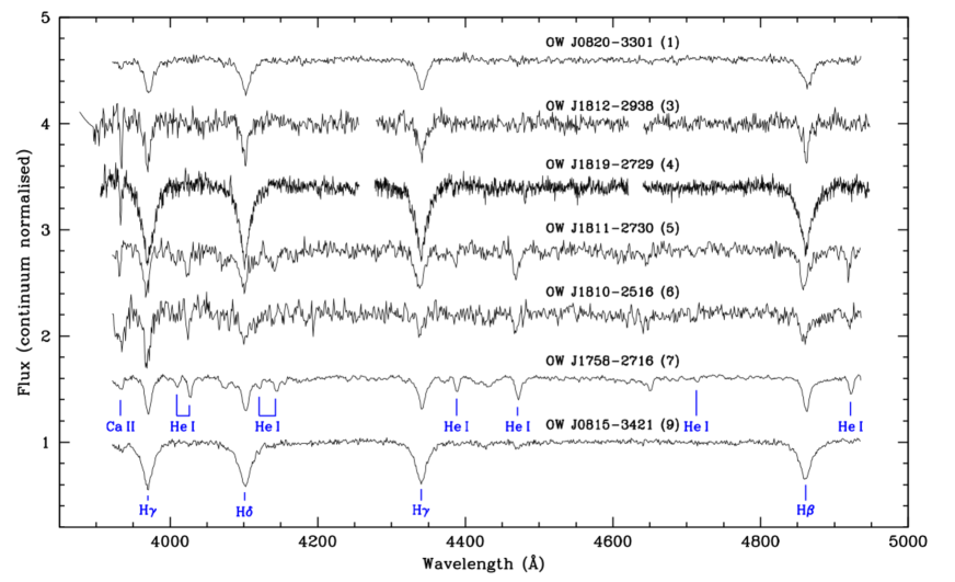
Figure 1: The continuum normalised SALT spectra of our targets where each spectrum has been shifted by +0.5 flux units. We note the wavelength of key lines in the spectra.

5 Individual objects

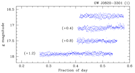
Figure 2: Light curves of OW J0820–3301 obtained with the SAAO 1-m telescope. The top light curve is shown at the correct brightness, whereas subsequent light curves (top-to-bottom) are displaced for display purposes only.

5.1 OW J082047.2–330107.8

The OW photometric observations of OW J082047.2–330107.8 (ID 1 in Table 1, and hereafter referred to as OW J0820–3301) showed evidence for periodic modulation on a period of 7.4 min and 0.13 mag in amplitude. We obtained followup photometry on four nights in Feb 2021 (Table 2) with a significant periodic signal on a period of 7.5 min on each occasion. The amplitude appears to be variable as does the significance of the period. In Fig. 2 we show these light curves: the amplitude of the modulation does change over time. An LS power spectrum (Fig. 3) shows an additional, less prominent, peak corresponding to a shorter period (5.7 min).

The multi-periodic nature of OW J0820–3301, and its high temperature (Table 5) are consistent with the properties of V361 Hya (or EC 14026) variables (Kilkenny et al., 1997; Heber, 2016; Lynas-Gray, 2021). Pulsation amplitudes in V361 Hya variables are typically less than 1% compared with nearly 10% in OW J0820–3301. However, several other V361 Hya variables have been observed with significant semi-amplitudes, including PG 1605+072 ($P$ = 8.0 min, $a\sim 0.064$ mag) (Koen et al., 1998), Balloon 090100001 ($P$ = 5.9 min, $a\sim 0.060$ mag) (Baran et al., 2009) and CS 1246 ($P$ = 6.2 min, $a\sim 0.025$ mag) (Barlow et al., 2010).

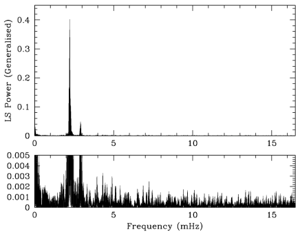
Figure 3: Generalised Lomb-Scargle power spectrum of OW J0820-3301.

Interestingly, the large amplitude oscillation observed in CS 1246 decayed to $a<0.005$ mag in the following eight years (Hutchens et al., 2017), while amplitude variations appear to be important in other V361 Hya variables (Reed et al., 2004; Kilkenny, 2010).

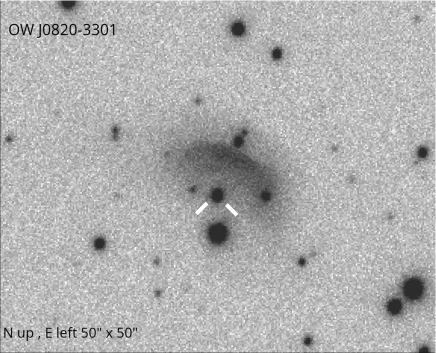
Figure 4: An image of the immediate field of OW J0820–3301 in H$\alpha$, combining three exposures taken during the VPHAS+ survey (Drew et al., 2014). It is 50${}^{\prime\prime}\times 50^{\prime\prime}$ wide and the target is in the center, indicated by the white dashes. An extended nebula lies to the north of OW J0820-3301.

The SALT spectrum of OW J0820–3301 obtained in 2016 (see details in Table 3) showed a nebular spectrum of a Strömgren sphere superimposed on broader Balmer absorption lines. After careful sky subtraction, the emission line spectrum was separated from the stellar spectrum. The latter is shown in Fig. 1. Fitting this spectrum indicates OW J0820–3301 has a temperature of $T_{\rm eff}$$\sim 37,400$K and $\log{g}$$\sim$5.7 (Table 5).

We performed a search for extended emission around our targets using the AAO/UKST H$\alpha$ and VPHAS+ (Drew et al., 2014) surveys and extracted an image for all sources. We found evidence for extended emission from around OW J0820–3301: in Fig. 4 we show an image taken in H$\alpha$ extracted from the VPHAS+ survey (Drew et al., 2014) which has higher resolution. The DECaPS survey shows the nebula as prominently in green colour, indicative of strong Oiii or H$\beta$ emission. Without more detailed spectroscopic observations across the nebula (and ideally integral field unit observations) we are unable to be certain that the nebula is associated with OW J0820–3301. However, using statistical arguments we can determine the likelihood that two ’interesting’ objects are located within (say) 2^′′ of each other. The Gaia EDR3 catalogue (Gaia Collaboration, 2021) shows 56 stars within 1^′ radius of OW J0820–3301 which are brighter than $G<19$ mag (85 for $G<$20 mag). The probability that this is a chance alignment is 0.03 percent ($G<19$) and 0.07 percent.

If OW J0820–3301 and the nebula are associated then we can estimate the age of the nebula. The Gaia EDR3 data (Gaia Collaboration, 2021) has a best fit distance to OW J0820–3301 of 3.7 kpc. The H$\alpha$ image shows a nebula which has a diameter along its semi-major axis of $\sim 8^{\prime\prime}$. For a distance of 3.7 kpc, simple geometry indicates a semi-major axis of $\sim$0.14 pc. If we assume a velocity of the expanding material to be 10–40 km s^-1 (Corradi & Schwarz, 1995) we find an age of the nebula of $\sim$3400–13600 years. More dedicated spectroscopic observations of the nebula are required.

5.2 OW J181227.9–293848.3

We identified OW J181227.9–293848.3 (ID 3 in Table 1, and hereafter referred to as OW J1812–2938) as having a very significant peak in its power spectrum at 10.8 min and an amplitude of 0.28 mag. No followup photometry was obtained of this source but we did obtain two spectra using SALT in 2016 (Table 3). We show the combined normalised spectrum in Fig. 1 which shows Balmer lines in absorption and a prominent Ca II absorption line.

Fitting this spectrum indicates OW J1812–2938 has a temperature $T_{\rm eff}$$\sim 31,000$K and $\log{g}$$\sim$4.7 (Table 5). These results, together with its period and amplitude, place it in the parameter range consistent with it being a BLAP, and we therefore designate it OW-BLAP-1.

5.3 OW J181920.9–272956.3

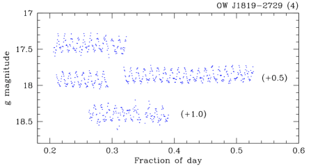
Figure 5: Light curves of OW J1819–2729 obtained with the SAAO 1-m telescope.

We identified OW J181920.9–272956.3 (ID 4 in Table 1, and hereafter referred to as OW J1819–2729) as having a very significant peak in its power spectrum at 15.7 min and an amplitude of 0.19 mag. We obtained followup photometry of this source using the SAAO 1.0m telescope on three nights with multiple 60 sec exposures on each occasion (c.f. Table 2). The light curves are shown in Fig.  5. These data confirm the 15.9 min period found from OW data although there is also a peak in the power spectra at half the 15.9 min period. There are some side-lobes of the main peak on the night of 2016-08-03 but this has the smallest number of photometric points. The folded light curves are sinusodial and symmetric.

We obtained spectra of OW J1819–2729 using SALT, SAAO 1.9m telescope and WHT. The longest series was obtained using the WHT where a series of 30 low resolution spectra were obtained. They were obtained at relatively high airmass (1.8–2.0) and the individual spectra were of low signal-to-noise ratio. However, the co-added spectra revealed Balmer absorption lines, with only marginal evidence for helium lines. The ratio of the equivalent width (Ca ii H+K, H${\epsilon}$) is consistent with an A-type spectrum.

The temperature ($T_{\rm eff}$$\sim$12,300 K) derived from the spectral fits (Table 5) is the lowest of the stars in our sample and is similar to the pulsating sdA stars (Bell et al., 2018). However, there is only one star in the Bell et al. (2018) set of new stars which has a period (4.6 min) which is even remotely close to that seen here but the amplitude of the pulsation of that star is $<$0.4 percent. These observations indicate that OW J1819–2729 is a possible sdAV variable star.

5.4 OW J181100.2–273013.3

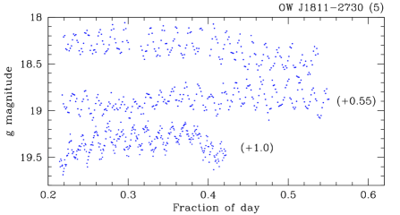
Figure 6: Light curves of OW J1811–2730 obtained with the SAAO 1-m telescope.

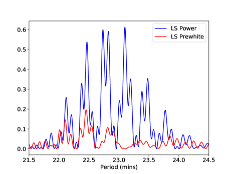
Figure 7: The Lomb-Scargle power spectrum of the combined light curve of OW J1811–2730 (after global trends have been removed) and the Lomb-Scargle power spectrum after the light curve has been pre-whitened by removing the period with maximum power.

OW J181100.2–273013.3 (ID 5 in Table 1, and hereafter referred to as OW J1811–2730) was observed on three occasions using the SAAO 1.0m telescope: at two epochs the exposure times were 120 sec and at one epoch 60 sec (Table 2). The light curves from the individual nights are shown in Fig. 6.

The period derived from each of the three nights is 22.7 – 22.9 min with an amplitude in the range 0.21–0.29 mag which is fully consistent with the 23.0 min and 0.21 mag from the OW survey data. To search for other periods in the light curve, we removed global trends in each night (which may have been due to differential colour terms between the comparison stars) and obtained a LS power spectrum (Fig. 7). There is evidence for the peaks in the power spectrum being split, but these largely disappear after pre-whitening on the period with peak power. We conclude there is little evidence for a second period in this source.

The mean spectrum shown in Fig. 1 shows the Balmer lines in absorption together with He i also in absorption. The spectral fits (Table 5) indicates OW J1811–2730 has a temperature $T_{\rm eff}\sim$27,000 K and log $g\sim$4.8. Together with the photometric properties indicates that OW J1811–2730 is a BLAP and we designate OW-BLAP2.

5.5 OW J181038.5–251608.6

We identified OW J181038.5–251608.6 (ID 6 in Table 1, and hereafter referred to as OW J1810–2516) as having a very significant peak in its power spectrum at 28.9 min and an amplitude of 0.42 mag. At $g$=19.6 mag it is the faintest target in our sample. We obtained one spectrum of OW J1810–2516 using SALT and the RSS and its normalised spectrum is shown in Fig. 1. Balmer lines are seen in absorption as are several lines due to helium. The fits to the spectra (Table 5) indicate a temperature $T_{\rm eff}\sim 30,000$K and $\log{g}$$\sim$4.2. Together with the period and amplitude we identify this as a BLAP and name it OW-BLAP-3.

5.6 OW J175848.2–271653.6

OW J175848.2–271653.6 (ID 7 in Table 1, OW J1758–2716) was reported as a variable with a period of 32.5 min and amplitude of 0.25 mag (Macfarlane et al, 2017a). The folded light curve indicated the source was similar to that of $\delta$ Sct stars. However, an optical spectrum indicated the star was more similar to a B spectral type than an A-F spectral type which would be expected from a $\delta$ Sct star. Intriguingly the phase folded light curve showed a curious ‘notch’ at peak brightness: we display the data reported in Macfarlane et al (2017a) folded on the main period in Fig. 8. Macfarlane et al (2017a) made the comparison between the notch observed here with the ‘Bump Cepheids’ (Mihalas, 2003). We obtained an additional set of 50 spectra taken on two nights in 2016 (see Table 3). Fitting the mean spectrum we find $T_{\rm eff}\sim 27,000$K and log g$\sim$4.2 (Table 5) and conclude that OW J1758–2716 is a BLAP and name it OW-BLAP-4.

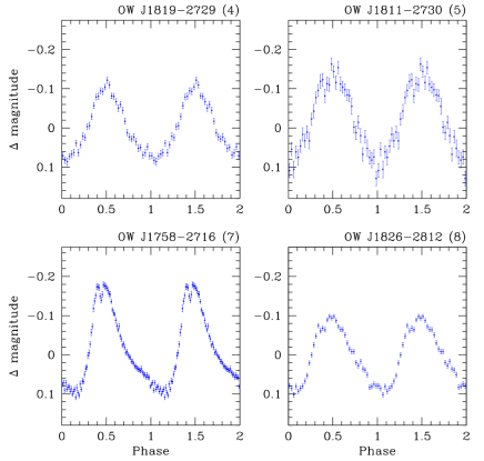
Figure 8: The phased and averaged light curves of OW J1819–2729 ($P$ = 15.715 min, top left), OW J1811–2730 ($P$ = 22.915 min, top right), OW J1758–2716 ($P$ = 32.00 min, bottom left) and OW J1826–2812 ($P$ = 32.960 min, bottom right).

5.7 OW J182628.4–2812019

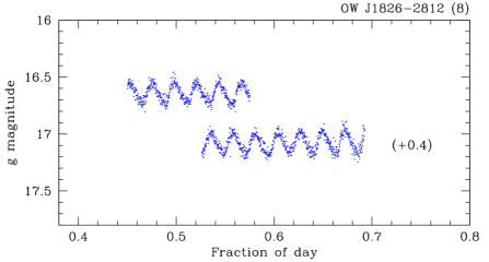
Figure 9: Light curves of OW J1826-2812 obtained using the SAAO 1-m telescope.

OW J182628.4–2812019 (ID 8 in Table 1, OW J1826–2812) was observed on two nights in May 2017 (Table 2) using the 1.0m telescope and SHOC. The period which we determine (32.9–33.0 min) is slightly longer than found using the original OW data (32.4 min) and with a higher amplitude ($\sim$0.18 mag compared to 0.12 mag). We show the light curves in Fig. 9 and the phase folded binned light curve in Fig. 8. There is a curious ‘ledge’ like feature just before maximum light. We return to this in §6. Spectroscopic observations are still required to determine the nature of this source.

5.8 OW J081530.8-342123.5

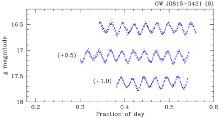
Figure 10: Light curves of OW J0815–3421 obtained with the SAAO 1-m telescope.

OW J081530.8–342123.5 (ID 9 in Table 1, and hereafter referred to as OW J0815–3421) has the longest apparent period of the candidate BLAPs shown in Table 1 (36.7 min) and an amplitude of 0.20 mag. Follow-up photometric observations were obtained on three nights in Feb 2021 (Table 2). A strong periodic signal was seen in the light curves with the LS periodogram indicating a period of 36.8 min which is consistent with the OW period. However, in Fig. 10 we show the individual light curves from these nights: there is evidence that the depth of every second minimum is deeper than the preceding minimum. This suggests that the true period, possibly an orbital ellipsoidal modulation, is 73.6 min.

We obtained a single spectrum of OW J0815–3421 in 2017 (Table 3) which showed the Balmer series in absorption (Fig. 1). A fit to this spectrum indicates a temperature and gravity consistent with that of an sdB star. To search for radial velocity variations we obtained a series of spectra using SALT in May 2021. This revealed a clear radial velocity variation (a semi-amplitude of 376$\pm$15 km s^-1) on a period of 73.6 min: we show the phase folded radial velocity curve in Fig. 11. A fit to the combined spectrum (made after accounting for the radial velocity variation of the individual spectra) indicates a temperature $T_{\mathrm{eff}}$ = $26,500\pm 1000$ K and $\log g$=$5.68\pm 0.15$.

We can now use this information to model and constrain the resulting stellar parameters using the photometric light curve using Lcurve, (see Copperwheat et al. (2011) for a detailed description). To model the system, we use a spherical star for the white dwarf and use a Roche geometry for the sdB companion. The free parameters in the model are the period ($P$), time of inferior conjunction ($t_{0}$), mass-ratio ($q$), inclination ($i$), the radii scaled by the semi-major axis ($r_{1,2}$), the effective temperature of both components ($T_{\mathrm{eff;1,2}}$), and the velocity scale ([$(K_{1}$ + $K_{2}$] $\sin{i}^{-1}$).

Ellipsoidal variations alone are not sufficient to fully constrain the binary parameters, and we therefore add priors and other model constraints. We use Gaussian priors on the sdB temperature as derived from the spectroscopy, surface gravity, and radial velocity semi-amplitude. We fix the limb and gravity darkening parameters using the tabulated values by Gianninas et al. (2013) and fix the beaming exponent to 1.62 (Loeb & Gaudi, 2003; Bloemen et al., 2011). For the white dwarf we use the approximation of the mass-radius relation of Eggleton from Verbunt & Rappaport (1988) to constrain the radius. First, the white dwarf radius cannot be smaller than the mass-radius relation. Second, we use a Gaussian prior to constrain the relative size of the white dwarf compared to the zero-temperature white dwarf relation to 10%. To find the best parameter values and uncertainties, we use a Markov-Chain Monte Carlo (MCMC) method as implemented in emcee (Foreman-Mackey et al., 2013). Before we fitted the model, we detrended and rescaled the uncertainties of the three individual lightcurves. We fit the combined lightcurve using 512 walkers and 2000 generations and show the resulting best fit and the folded light curve in Fig. 12 and the resulting best fit parameters with their associated errors in Table 4.

The mass of the white dwarf is $\sim$0.7$M_{\odot}$  ($T_{\rm eff}\sim 14,000$ K) whilst the mass of the sdB star is $\sim$0.34$M_{\odot}$  ($T_{\rm eff}\sim 26,500$K). The component masses and orbital period of (73.7 min), make it similar to the well known white dwarf, sdB binary CD–30^∘ 11223 which has an orbital period of 70.5 min (Vennes et al., 2012) and PTF1 J2238+7430 the recently discovered white dwarf, sdB binary (Kupfer et al., 2022). The recent catalogue of post common enevlope binaries of Kruckow et al. (2021) lists five white dwarf, sdB binaries with an orbital period shorter than 80 min: OW J0815-3421 is now the sixth such binary. The mass of the component stars are similar to ZTF J2320+3750 (55.25 min) (Burdge et al., 2020a) and ZTF J2055+4651 (56.35 min) (Kupfer et al., 2020).

The finding that OW J0815–3421 is a binary indicates that medium resolution spectroscopic observations made over several days could reveal evidence for binarity in the other sources identified in this survey (c.f. the comments of Byrne & Jeffery (2020) on the Roche-lobe overflow model for the formation of BLAPs).

t0 (HJD)	$2459267.432196$(26)
$P$ (d)	$0.0511843$(16)
$q$	$0.493^{+0.061}_{-0.072}$
$i$ (∘)	$83.14^{+4.60}_{-10.55}$
$M_{1}$ ($M_{\odot}$)	$0.707^{+0.086}_{-0.082}$
$M_{2}$ ($M_{\odot}$)	$0.343^{+0.076}_{-0.066}$
$R_{1}$ ($R_{\odot}$)	$0.01189^{+0.0012}_{-0.0011}$
$R_{2}$ ($R_{\odot}$)	$0.216^{+0.018}_{-0.015}$
$a$ ($R_{\odot}$)	$0.590^{+0.027}_{-0.027}$
$T_{1}$ (K)	$14077^{+11290}_{-6233}$
$T_{2}$ (K)	$26461^{+1052}_{-965}$
$\log g_{2}$	$5.44^{+0.021}_{-0.028}$

Table 4: The system parameters derived for OWJ0815–3421 using Lcurve to model the light curve.

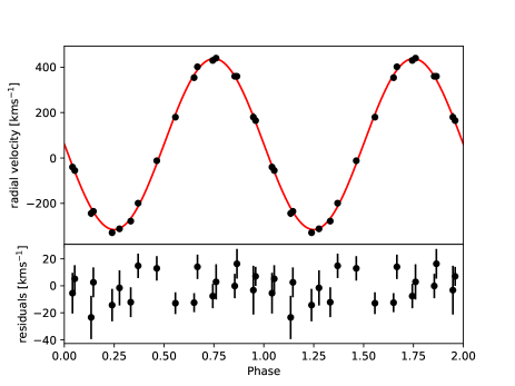
Figure 11: Upper panel: The radial velocity data of OW J0815–3421 phased on the binary orbital period of 73.7 min together with the best fit sinusoid. The lower panel: the residuals to the fit. Two orbits are shown for better visualisation.

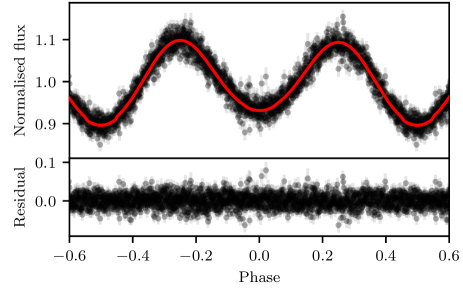
Figure 12: The data of OW J0815–3421, shown in black, has been phased on a period of 73.71 min. The red solid line shows the fit to the data made using Lcurve. The data have been repeated to cover two cycles and phase 0.0 represents the secondary minimum.

ID	Name	$T_{\rm eff}$ (K)	$\log g$	$\log n_{\rm(He/H)}$	Classification	New designation
1	OW J0820-3301	$37\,400\pm 1500$	$5.71\pm 0.11$	$-2.5\pm 0.3$	V361 Hya
3	OW J1812-2938	$30\,600\pm 2500$	$4.67\pm 0.25$	$-2.1\pm 0.2$	BLAP	OW-BLAP-1
4	OW J1819-2729	$12\,300\pm\ \ 500$	$4.81\pm 0.20$	$-0.6\pm 0.2$	sdAV
5	OW J1811-2730	$27\,300\pm 1500$	$4.83\pm 0.20$	$-0.7\pm 0.1$	BLAP	OW-BLAP-2
6	OW J1810-2516	$29\,900\pm 3500$	$4.16\pm 0.40$	$-0.8\pm 0.3$	BLAP	OW-BLAP-3
7	OW J1758-2716	$27\,300\pm 2000$	$4.20\pm 0.20$	$-0.8\pm 0.2$	BLAP	OW-BLAP-4
9	OW J0815-3421	$26\,500\pm 1000$	$5.68\pm 0.15$	$-2.8\pm 0.2$	sdB

Table 5: The results of spectral fits to optical spectra of the candidate BLAPs, including the best fit effective temperature, surface gravity and helium-to-hydrogen abundance ratio. The penultimate column shows the likely variable star classification.

6 Discussion

Of the nine sources which we identified as candidate BLAPs (Table 1), four have characteristics consistent with being a BLAP. The key was obtaining spectra with sufficient spectral resolution ($R\sim$2000) to be able to fit the absorption lines and hence obtain sufficiently constrained values for temperature and gravity. Follow-up high time-resolution photometry was essential in identifying OW J0815–3412 as a very short period binary containing a sdB star and also identifying the notch feature in four objects, two of which are BLAPs. We note that the derived periods from follow-up photometry are consistent with the initial periods derived from the OW survey. We now discuss all sources reported in this study in the wider context.

6.1 Comparison of BLAPs with other short period variables using the Gaia HRD

The simplest and most readily available means of comparing the colour and luminosity of different types of sources is through the Gaia HRD based on ($(BP-RP),MG$) data. Since the OW and the ZTF surveys observed fields close to the Galactic plane, the extinction can be high and can show changes on relatively small spatial scales ($<1^{\prime}$). We therefore de-redden the Gaia ($(BP-RP),MG$) data of variable stars of different types using Bayestar19 (Green et al., 2019).

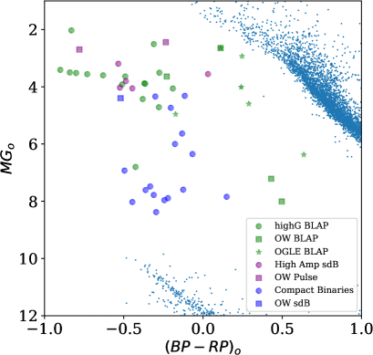
Figure 13: The observed $(BP-RP)_{o}$, $MG_{o}$ colour-absolute magnitudes for the BLAPs and other high amplitude pulsators as identified in the OW survey. For comparison we also show the position of the high gravity BLAPs reported in Kupfer et al. (2019, 2021); compact binaries identified in Burdge et al. (2020a, b); and high amplitude sdB stars.

There are a number of different classes of variable stars which lie in the region of the Gaia HRD where BLAPS have been found (Ramsay, 2018; McWhirter & Lam, 2022). For instance, strongly magnetic Cataclysmic Variables (also known as Polars) can show high (up to 1 mag) variation over their orbital period, but their orbital periods are $\buildrel{\lower 3.0pt\hbox{$>$}}\over{\lower 2.0pt\hbox{$\sim$}}$80 min. In contrast, the interacting double degenerate AM CVn binaries have orbital periods $\buildrel{\lower 3.0pt\hbox{$<$}}\over{\lower 2.0pt\hbox{$\sim$}}$1 hr but have amplitudes $<$0.1 mag. We therefore include for comparison a number of short period binaries (6.9< $P_{\rm orb}<$56.4 min) which consist of degenerate stars and can show high amplitudes of variability, many of which also show eclipses (Burdge et al., 2020a, b) and a small sample of high amplitude sdB stars which have high amplitudes and short periods. In addition we add the high gravity BLAPs reported by Kupfer et al. (2019) and also the high gravity ‘sdB’ pulsators reported in Kupfer et al. (2020). Since the periods of these systems are similar, with the latter sample showing only slightly lower amplitudes, we class both these samples as high gravity BLAPs, although they may have a different internal structure. We also take the sources originally reported by Pietrukowicz et al. (2017) and have Dec$>-30^{\circ}$ and hence the reddening can be determined using Bayestar19. In Fig. 13 we show the location of these stars in the ($(BP-RP)_{o},M_{G_{o}}$) plane and for comparison stars which are within 50 pc of the Sun, which we assume have negligible reddening.

As can be seen, the sources cover a wide range in the Gaia HRD, encompassing the area bluer than the main sequence but more luminous than the main white dwarf cooling tracks. The BLAPs have a wide range of $M_{G_{o}}$ although we caution that because the error on their parallax is generally high the resulting uncertainty on $M_{G_{o}}$ can be up to $\sim$1 mag (c.f. Table 1). The compact binaries tend to be less luminous compared to the other classes with those being more luminous having an sdB star as a binary component. Stellar pulsators appear to be more luminous. However, it is not possible to determine the nature of any given source based on its location purely in the Gaia HRD.

Fortunately, for seven of the sources in this study we have been able to determine their temperature and gravity (Table 5). In Fig. 14 we show the location of the OW BLAPs, the BLAP sample from Pietrukowicz et al. (2017) and the high gravity BLAPs from Kupfer et al. (2019). We also show the evolutionary tracks for stars of different mass taken from Kupfer et al. (2019). The OW BLAPS share a similar part of the $T_{\rm eff}$,$\log{g}$  plane (relatively low gravity) whilst the high gravity BLAPS have a shorter pulsation period and high gravity.

6.2 Notch feature at maximum brightness

Macfarlane et al (2017a) identified a dip in the light curve of OW J1758–2716 occuring near maximum light which was compared to features seen in ‘Bump’ Cepheid variables. These bumps are features in the phase folded light curve which occur on the rise to maximum brightness or in the descent from brightness. The phase of where this occurs is known as the Hertzsprung Progression (Hertzsprung, 1926; Bono et al., 2000) and depends on stellar mass and therefore the observed period. There are Cepheids which show a dip at flux maximum very similar to what we observe in OW J1758–2716, see for example RU Dor (Fig 9, Plachy et al. (2021)). It is likely that Bump features are due to a resonance between the fundamental pulsation mode and the second overtone (e.g. Gastine & Dintrans (2008) and references therein).

We do not have additional photometric observations since those reported by Macfarlane et al (2017a) which showed photometry covering a timeline of $\sim$160 min. Further observations would be required to search for a second over-tone in the light curve. However, as shown in Fig. 8, OW J1811–2730 and OW J1826–2812 show hints for a slight bump in their folded light curves on the rise to maximum brightness. There is no sign of bump features in the high gravity BLAPs identified by Kupfer et al. (2019).

6.3 sdA pulsators

High-gravity A stars (sdA’s) have been widely discussed since being identified in the Sloan Digital Sky Survey with H-dominated spectra, $9000>T_{\rm eff}>6500$ K), and $6.5>\log g>5.5$ (Kepler et al., 2016). Whilst purely a spectroscopic classification, they have been identified with binaries of a subdwarf and a main sequence object of type FGK; main sequence A stars with a high surface gravity; or extremely low-mass white dwarfs (ELMs) or their precursors (pre-ELMs). Of these only the latter (ELMs and pre-ELMs) stand scrutiny (Pelisoli et al., 2016; Bell et al., 2018).

Bell et al. (2018) in their search for pulsating sdA stars found three pre-ELM candidates which have temperatures ($\sim$8,000 K) which are slightly cooler than that measured for OW J1819–2729. They indicate that pre-ELM stars might undergo CNO flashes on a short timescale. Byrne & Jeffery (2020) studied the pulsation properties of pre-ELMs and ELMs as they evolve from the subgiant branch, where they must lose mass to a close companion, onto the ELM white dwarf sequence. Their models included chemical diffusion, and demonstrated how opacity from concentrated iron-group elements can switch on pulsations in pre-ELM models exactly where BLAPs had previously been identified (Pietrukowicz et al., 2017; Kupfer et al., 2019). A few models with core masses $0.255\leq M_{\rm core}\leq 0.305$ $M_{\odot}$ show a late hydrogen-shell flash after becoming an ELM. This flash inflates the white dwarf causing a loop in the evolution track which passes through the $T_{\rm eff}$,$\log{g}$  plane in the region occupied by OW J1819–2729. During this time the models are also unstable to pulsation, with periods approximately between 200 and 4000 s ($\log g$ between 6.0 and 4.0).

Difficulties with this argument include the short time that models spend in such flash-driven loops, and the expectation that, in order to become an ELM, the agency of a companion is required. Nevertheless, further evidence to test the notion that OW J1819–2729 is a shell-flashing ELM should be sought.

6.4 Space Density of BLAPs

The OW survey covered 404 distinct fields each covering one square degree. We have identified four stars which have short photometric periods and high amplitudes with followup spectroscopic observations indicate they are BLAPs, implying one BLAP per $\sim$0.01 deg^-1. Byrne et al. (2021) made predictions of how many BLAPs would be expected in our Galaxy using the Binary Population Spectral Synthesis code (Eldridge et al., 2017). They found the numbers were very dependent on Galactic latitude (concentrated towards the plane) and longitude (highest the Bulge) although regions of high extinction could make this very variable. Regions with the highest concentrations of predicted BLAPs reach $\sim$0.3 deg^-1 at a depth of $g$=20 mag, but a median of 0.001 deg^-1 at $b$=$0^{\circ}$. Moving to $b$=$15^{\circ}$ results in a very low number of BLAPs being predicted. Our search for BLAPs in the OW survey did not reach as faint as $g$=20 mag but with an observed number density of $\sim$0.01 deg^-1 down to $g\sim 19$, our findings appear reasonably consistent with the predictions of Byrne et al. (2021), giving good grounds to suggest that 12,000 BLAPs may exist in our Galaxy.

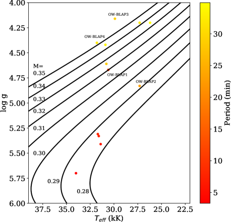
Figure 14: The solid lines are predicted evolutionary tracks for BLAPs in the T_eff, log $g$ plane and taken from Kupfer et al. (2019) for stars of different masses. The BLAPs identified in the OW survey are indicated where the colour of the symbol indicates the stars pulsation period. The shorter period BLAPs come from the sample of Pietrukowicz et al. (2017) while the longer period (and high gravity) systems are from the sample of Kupfer et al. (2019). The OW BLAPs share a similar part of the plane as the lower gravity sample of Pietrukowicz et al. (2017).

7 Conclusion

We have used data taken as part of the OmegaWhite survey to search for short period, high amplitude variables which may be BLAPs: we identified nine stars which we initially classed as candidate BLAPs. Using a combination of followup photometry, spectroscopy and Gaia data we were able to identify four of these variables as BLAPs, one of these being previously identified as a BLAP by Pietrukowicz et al. (2017). Overall they have similar properties to the BLAPs identified by Pietrukowicz et al. (2017) rather than the high gravity BLAPs identified by Kupfer et al. (2019, 2021).

We have also identified OW J0815–3421 as a binary system containing an sdB and a low mass star. With an orbital period of 73.7 min, it is one of half a dozen white dwarf - sdB star binaries with orbital periods shorter than 80 min. A more detailed investigation is required to determine if it is a double-detonation thermonuclear supernova progenitor like PTF1 J2238+7430 (Kupfer et al., 2022). OW J1819–2729 is a pulsating sdAV star which has interesting properties which makes future modelling an interesting future study. One further source, OW J0820–3301, is a V361 Hya pulsator which has an extended nebula which is spatially nearby. Although at this point we cannot be certain it is physically associated with the short period variable, further observations using an integral field spectrograph maybe able to determine if there is any association between the nebula and the variable star.

Finally we note that high cadence observations of these short period variable stars have revealed detailed structure in their folded light curve. We make comparison with other types of pulsating variable stars which show similar features in their light curves. We encourage stellar modellers to reproduce such features using appropriate models.

8 Acknowledgments

The targets identified in this paper were identified in data obtained using the ESO VST and OmegaCam under proposals: 088.D-4010; 090.D-0703; 091.D-0716; 092.D-0853; 093.D-0753; 093.D-0937; 094.D-0502; 095.D-0315; 096.D-0169; 097.D-0105; 098.D-0130; 099.D-0164 and 0100.D-0066. SALT spectroscopic data were obtained under proposals: 2015-2-SCI-035; 2016-1-DDT-004; 2016-1-MLT-010; 2016-1-SCI-015 and 2017-2-SCI-051. This paper uses observations made at the South African Astronomical Observatory and the South African Large Telescope and we thank the staff at both for their expertise in obtaining these data. Based on observations made with the WHT (programme ID: W/16B/N4) operated on the island of La Palma by the Isaac Newton Group of Telescopes in the Spanish Observatorio del Roque de los Muchachos of the Instituto de Astrofísica de Canarias. PAW acknowledges support from UCT and the NRF. TK acknowledges support from the National Science Foundation through grant AST #2107982, from NASA through grant 80NSSC22K0338 and from STScI through grant HST-GO-16659.002-A. PJG acknowledges support from NOVA for the original OmegaWhite observations in the Dutch VST/Omegacam GTO observations. PJG is supported by NRF SARChI Grant 111693. Armagh Observatory and Planetarium is core funded by the Northern Ireland Executive through the Department for Communities. UH and AI acknowledge funding by the Deutsche Forschungsgemeinschaft (DFG) through grants HE1356/70-1 and HE1356/71-1. We thank Kinwah Wu for a useful discussion on probabilities of stars being spatially nearby and Evan Bauer who generated the evolutionary tracks shown in Fig. 14. We thank Steven Hämmerich for providing us with synthetic spectra for solar metal composition. We thank the referee for a useful report.

Data Availability

The images obtained as part of the OW survey can be accessed through the ESO portal. Light curves and spectra can be obtained via a reasonable request from the authors.

References

- Alard & Lupton (1998) Alard, C., Lupton, R. H., 1998, ApJ, 503, 325
- Astraatmadja & Bailer-Jones (2016) Astraatmadjam, T. L., & Bailer-Jones, C. A. L., 2016, ApJ, 833, 119
- Bailer-Jones (2015) Bailer-Jones, C. A. L., 2015, PASP, 127, 994
- Baran et al. (2009) Baran, A., et al., 2009, MNRAS, 392, 1092
- Barlow et al. (2010) Barlow, B. N. et al., 2010, MNRAS, 403, 324
- Bell et al. (2018) Bell, K. J., et al., 2018, A&A, 617, A6
- Bellm et al. (2019) Bellm, E. C., et al., 2019, PASP, 131, 018002
- Bloemen et al. (2011) Bloemen, S., et al., 2011, MNRAS, 410, 1787
- Bono et al. (2000) Bono, G., Marconi, M., Stellingwerf, R. F., 2000, A&A, 360, 245
- Burdge et al. (2020a) Burdge, K., et al., 2020a, ApJ, 905, 32
- Burdge et al. (2020b) Burdge, K., et al., 2020b, ApJ, 905, L7
- Butler & Giddings (1985) Butler, K. and Giddings, J. R., 1985, Newsletter of Analysis of Astronomical Spectra, 9, Univ. London
- Byrne & Jeffery (2018) Byrne, C. M., Jeffery, C. S., 2018, MNRAS, 481, 3810
- Byrne & Jeffery (2020) Byrne, C. M., Jeffery, C. S., 2020, MNRAS, 492, 232
- Byrne et al. (2021) Byrne, C. M., Stanway, E. R., Eldridge, J. J., 2021, MNRAS, 507, 621
- Chambers et al. (2016) Chambers, K C., et al., 2016, arXiv-1612.05560
- Coppejans et al. (2013) Coppejans, R., Gulbis, A. A. S., Kotze, M. M. et al., 2013, PASP, 125, 976
- Copperwheat et al. (2011) Copperwheat, C. M., et al., 2011, MNRAS, 410, 1113
- Corradi & Schwarz (1995) Corradi, R. L. M., Schwarz, H. E. 1995, A&A, 293, 871
- Drake et al. (2013) Drake, A. J., et al. 2013, AJ, 763, 32
- Drew et al. (2014) Drew, J. E., Gonzalez-Solares, E., Greimel, R., et al., 2014, MNRAS, 440, 2036
- Eldridge et al. (2017) Eldridge J. J., Stanway E. R., Xiao L., McClelland L. A. S., Taylor G., Ng M., Greis S. M. L., Bray J. C., 2017, Publ. Astron. Soc. Australia, 34, e058
- Foreman-Mackey et al. (2013) Foreman-Mackey, D., Hogg, D. W., Lang, D., Goodman, J., 2013, PASP, 125, 306
- Gaia Collaboration (2018) Gaia Collaboration, Luri, X., Brown, A. G. A., et al., 2018, A&A, 616, A9
- Gaia Collaboration (2021) Gaia Collaboration, Brown, A.G.A., et al., 2021, A&A, 649, A1
- Gastine & Dintrans (2008) Gastine, T., Dintrans, B., 2008, A&A, 490, 743
- Gianninas et al. (2013) Gianninas, A., Strickland, B. D., Kilic, M., et al. 2013, ApJ, 766, 3
- Giddings (1981) Giddings, J. R., 1981, PhD thesis, University of London
- Graham et al (2019) Graham, M. J., et al., 2019, PASP, 131, 078001
- Green et al. (2018) Green, G. M., Schlafly, E. F., Finkbeiner, D., et al., 2018, MNRAS, 478, 651
- Green et al. (2019) Green, G. M., et al., 2019, ApJ, 887, 93
- Hartman et al. (2008) Hartman J. D., Gaudi B. S., Holman M. J., McLeod B. A., Stanek K. Z., Barranco J. A., Pinsonneault M. H., Kalirai J. S., 2008, ApJ, 675, 1254
- Heber (2016) Heber, U., 2016, PASP, 128, h2001
- Hertzsprung (1926) Hertzsprung, E., 1926, BAN, 3, 115
- Hutchens et al. (2017) Hutchens, Z. L., Barlow, B. N., Vasquez Soto, A., Reichart, D. E., Haislip, J. B., Kouprianov V. V., Linder, T. R., & Moore, J. P., 2017, Open Astronomy, 26, 252
- Irrgang et al. (2018) Irrgang, A., Kreuzer, S., Heber, U., Brown, W., 2018, A&A, 615, L5
- Kepler et al. (2016) Kepler, S. O., Pelisoli, I., Koester, D., et al., 2016, MNRAS, 455, 3413
- Kilkenny et al. (1997) Kilkenny, D, Koen, C., O’Donoghue, D., Stobie, R. S., 1997, MNRAS, 285, 640
- Kilkenny (2010) Kilkenny, D., 2010, Ap&SS, 329, 175
- Kobulnicky et al. (2003) Kobulnicky H. A., Nordsieck K. H., Burgh E. B., Smith M. P., Percival J. W., Williams T. B., O’Donoghue D., 2003, in Iye M., Moorwood A. F. M., eds, Proc. SPIE Conf. Ser. Vol. 4841, Instrument Design and Performance for Optical/Infrared Ground-based Telescopes. SPIE, Bellingham, 1634
- Kruckow et al. (2021) Kruckow, M. U., Neunteufel, P. G., Di Stefano, R., Gao, Y., Kobayashi, C., 2021, ApJ, 920, 86
- Koen et al. (1998) Koen, C., O’Donoghue, D., Kilkenny, D., Lynas-Gray, A. E., Marang, F., & van Wyk, F., 1998, MNRAS, 296, 317
- Kupfer et al. (2019) Kupfer, T., et al., 2019, ApJ, 878, L35
- Kupfer et al. (2020) Kupfer, T., et al., 2020, ApJL, 898, L25
- Kupfer et al. (2021) Kupfer, T., et al., 2021, MNRAS, 505, 1254
- Kupfer et al. (2022) Kupfer, T., et al., 2022, ApJ, 925, L12
- Kurucz (1996) Kurucz, R., Astronomical Society of the Pacific Conference Series, 108, 160
- Loeb & Gaudi (2003) Loeb, A., Gaudi, B. S., 2003, ApJ, 588, L117
- Lynas-Gray (2021) Lynas-Gray, A. E., 2021, Frontiers in Astronomy and Space Sciences, 8, 19
- Macfarlane et al. (2015) Macfarlane, S. A., Toma, R., Ramsay, G., et al., 2015, MNRAS, 454, 507
- Macfarlane et al (2017a) Macfarlane S. A. et al., 2017a, MNRAS, 465, 434
- Macfarlane et al. (2017b) Macfarlane S. A. et al., 2017b, MNRAS, 470, 732
- McWhirter & Lam (2022) McWhirter, P. R., Lam, M. C., 2022, MNRAS, 511, 4971
- Mihalas (2003) Mihalas D., 2003, in Hubeny I., Mihalas D., Werner K., eds, ASP Conf. Ser. Vol. 288, Stellar Atmosphere Modeling. Astron. Soc. Pac., San Francisco, p. 471
- Napiwotzki et al. (2004) Napiwotzki, R. et al., 2004, Astrophysics and Space Science, 291, 321
- Naslim et al. (2013) Naslim, N., Jeffery, C. S., Hibbert, A., Behara, N. T., 2013, MNRAS, 434, 1920
- Pelisoli et al. (2016) Pelisoli, I., Kepler, S. O., Koester, D., & Romero, A. D., 2016, ‘20th European White Dwarf Workshop’, eds. P.E. Tremblay, B. Gänsicke, and T. Marsh, ASP Conference Series, Vol. 509, p. 447, San Francisco
- Pietrukowicz et al., (2015) Pietrukowicz P. et al., 2015, AcA, 65, 63
- Pietrukowicz et al. (2017) Pietrukowicz, P. et al., 2017, NatAs, 1, 166
- Plachy et al. (2021) Plachy, E., et al.,2021, ApJS, 253, 11
- Press et al (1992) Press W.H., Teukolsky S.A., Vetterling W.T., Flannery B.P., 1992, Numerical Recipes in C, 2nd ed., New York, Cambridge University Press
- Przybilla et al. (2011) Przybilla, N., Nieva, M-F., Butler, K., 2011, JPhCS, 328a2015P
- Ramsay (2018) Ramsay, G., 2018, A&A, 620, L9
- Reed et al. (2004) Reed, M., et al., 2004, MNRAS, 348, 1164
- Romero et al. (2018) Romero, A. D., Córsico, A. H, Althaus, L. G., et al., 2018, MNRAS, 477, L30
- Schaffenroth et al. (2021) Schaffenroth, V.,Casewell, S. L., Schneider, D., Kilkenny, D., Geier, S., Heber, U, Irrgang, A., Przybilla, N., Marsh, T. R., Littlefair, S. P., Dhillon, V. S., 2021, MNRAS, 501, 3847
- Shappee et al. (2014) Shappee, B. J., et al., 2014, ApJ, 788, 48
- Taylor (2006) Taylor, M. B., 2006, ASPC, 351, 666, in Astronomical Data Analysis Software and Systems XV, eds. C. Gabriel et al.
- Toma et al. (2016) Toma, R. et al., 2016, MNRAS, 463, 1099
- Udalski et al. (2015) Udalski, A., Szymański, M. K., Szymański, G., 2015, AcA, 65, 1
- Vennes et al. (2012) Vennes, S., Kawka, A., O’Toole, S. J., Németh, P., & Burton, D. 2012, ApJL, 759, L25
- Verbunt & Rappaport (1988) Verbunt, F., Rappaport, S., 1988, ApJ, 332, 193
- Wozniak (2000) Wozniak, P. R., 2000, AcA, 50, 421
- Zechmeister & Kürster (2009) Zechmeister, M. & Kürster, M., 2009, A&A, 496, 577