The chirality-dependent second-order spin current
in systems with time-reversal symmetry

Abstract

Spin currents proportional to the first- and second-order of the electric field are calculated in a specific tight-binding model with time-reversal symmetry. Specifically, a tight-binding model with time-reversal symmetry is constructed with chiral hopping and spin-orbit coupling. The spin conductivity of the model is calculated using the Boltzmann equation. As a result, it is clarified that the first-order spin current of the electric field vanishes, while the second-order spin current can be finite. Furthermore, the spin current changes its sign by reversing the chirality of the model. The present results reveal the existence of spin currents in systems with time-reversal symmetry depending on the chirality of the system. They may provide useful information for understanding the chirality-dependent spin polarization phenomena in systems with time-reversal symmetry.

I Introduction

Three-dimensional structures that do not have mirror symmetry are called chiral. This symmetry breaking gives rise to various physical properties such as electrical magnetochiral effect [1] and chiral soliton lattice [2], which will be useful for spintronics or magnetic devices. Among these properties, the spin polarization phenomenon called ‘chirality-induced spin selectivity’ (CISS) has recently attracted much attention [3, 4]. CISS was first discovered in DNA in 2011 [5, 6] and has been intensively studied in organic molecules. CISS in DNA was reported to produce spin polarization rates of up to $60\text{\,}\%$ [5] and is expected to be applied to efficient spin current generation techniques in the future. In 2020, it was shown that the inorganic crystal CrNb3S6 also shows CISS [7, 8]. More recently, CISS was confirmed also in inorganic crystals such as NbSi2 and TaSi2 [9].

While the theory of CISS in organic materials has been intensively investigated [10], that in inorganic materials has not been explored. Because the CISS is observed in the paramagnetic phase [7, 9], the spin polarization occurs in the states with time-reversal symmetry. However, it is known that a spin current linear in the electric field does not arise in single-channel systems with time-reversal symmetry [11]. This theorem makes the construction of the CISS theory difficult.

In this study, we construct a chiral tight-binding model with time-reversal symmetry and evaluate the spin conductivity in the first- and second-order with respect to the electric field. Specifically, we study a tight-binding model with chiral hopping and spin-orbit coupling to calculate the spin conductivity using the Boltzmann transport equation. We show that the first-order spin conductivity vanishes in the tight-binding model, while the second-order spin conductivity can be finite. Furthermore, the spin conductivity changes its sign by reversing the chirality of the model. The present results reveal the existence of spin currents in systems with time-reversal symmetry and the existence of chirality-dependent spin currents. They provide useful information for understanding the chirality-dependent spin polarization phenomena in systems with time-reversal symmetry.

This paper is organized as follows. In Sect. II, we start with symmetry analysis of spin conductivities in the first- and second-order with respect to the electric field in the Hamiltonians with time-reversal symmetry. In Sect. III, we introduce a specific chiral tight-binding model and calculate the chirality dependence of the second-order spin conductivity. We also discuss the parameters required for the chirality-dependent spin conductivity to arise. Section IV is devoted for discussions and conclusions.

II Symmetry Analysis

We first discuss whether the spin current flows when time-reversal symmetry is imposed on the Hamiltonian in general. We consider a model that is diagonal with respect to the spin but includes sublattice degrees of freedom, i.e., we assume that the spin $s_{z}$ ($s_{z}=\uparrow,\downarrow$) along the $z$-axis is a good quantum number. In this case, the Hamiltonian in the wavenumber representation can be written as

$$\mathcal{H}({\bf\it k})=\begin{pmatrix}\mathcal{H}({\bf\it k},\uparrow)&O\\ O&\mathcal{H}({\bf\it k},\downarrow)\\ \end{pmatrix},$$ (1)

where $\mathcal{H}({\bf\it k},\uparrow)$ and $\mathcal{H}({\bf\it k},\downarrow)$ are matrices whose matrix elements are between the band index $n$.

By solving the Boltzmann transport equation within the approximation of constant relaxation time, the spin-resolved first-order conductivity $\sigma_{zz}(s_{z})$ and spin-resolved second-order conductivity $\sigma_{zzz}(s_{z})$ with respect to the electric field $E_{z}$, i.e., $j_{z}(s_{z})=\sigma_{zz}(s_{z})E_{z}+\sigma_{zzz}(s_{z}){E_{z}}^{2}+\cdots$, can be written as [12]

$$\sigma_{zz}(s_{z}) =\frac{e^{2}\tau}{\hbar^{2}}\sum_{n}\int_{\mathrm{BZ}}\frac{\differential^{3}k}{(2\pi)^{3}}\ \frac{\partial^{2}\varepsilon_{n}({\bf\it k},s_{z})}{{\partial k_{z}}^{2}}f(\varepsilon_{n}({\bf\it k},s_{z})),$$ (2)

$$\sigma_{zzz}(s_{z}) =\frac{e^{3}\tau^{2}}{\hbar^{3}}\sum_{n}\int_{\mathrm{BZ}}\frac{\differential^{3}k}{(2\pi)^{3}}\ \frac{\partial^{3}\varepsilon_{n}({\bf\it k},s_{z})}{{\partial k_{z}}^{3}}f(\varepsilon_{n}({\bf\it k},s_{z})),$$ (3)

where $e(<0)$ is the electric charge, $\tau$ represents the relaxation time, $\varepsilon_{n}({\bf\it k},s_{z})$ represents the eigenenergy of the band index $n$ with wave number ${\bf\it k}$ and spin $s_{z}$, and $f(\varepsilon)$ represents the Fermi distribution function. $\int_{\mathrm{BZ}}\differential^{3}k$ means the integration over the entire Brillouin zone. The first-order spin conductivity $\sigma^{\mathrm{s}}_{zz}$ and the second-order spin conductivity $\sigma^{\mathrm{s}}_{zzz}$ are defined as

$$\sigma^{\mathrm{s}}_{zz} =\sigma_{zz}(\uparrow)-\sigma_{zz}(\downarrow),$$ (4)

$$\sigma^{\mathrm{s}}_{zzz} =\sigma_{zzz}(\uparrow)-\sigma_{zzz}(\downarrow).$$ (5)

We further suppose that the Hamiltonian in Eq. (1) has the time-reversal symmetry that can be written as $\Theta=-is_{y}K$, where $K$ is the complex conjugate operator. In this case, the eigenenergy of the Hamiltonian in Eq. (1) satisfies

$$\varepsilon_{n}({\bf\it k},s_{z})=\varepsilon_{n}(-{\bf\it k},-s_{z}).$$ (6)

Using this equation in Eqs. (2) and (3), we can readily see that

$$\sigma_{zz}(s_{z}) =\sigma_{zz}(-s_{z}),$$ (7)

$$\sigma_{zzz}(s_{z}) =-\sigma_{zzz}(-s_{z}),$$ (8)

which means that the first-order spin conductivity $\sigma^{\mathrm{s}}_{zz}$ vanishes in systems satisfying the above time reversal symmetry, while the second-order spin conductivity $\sigma^{\mathrm{s}}_{zzz}$ can be finite even under such conditions. Note that this argument does not hold if the degrees of freedom of the time-reversal operator except for spin, for example, the sublattice degrees of freedom are not an identity matrix.

III Model Analysis

Next, we discuss the chirality dependence of the second-order spin conductivity in a specific tight-binding model. We introduce a three-dimensional tight-binding model with chiral hopping shown in Fig. 1 [13]. This model consists of two-dimensional honeycomb lattices stacked along the $z$-axis. The Hamiltonian can be written as

$$H =H_{\mathrm{hop}}+H_{\mathrm{chiral}}+H_{\mathrm{SOC}},$$ (9)

$$H_{\mathrm{hop}} =t_{1}\sum_{\langle i,j\rangle,l,\alpha}c_{i,l,\alpha}^{\dagger}c_{j,l,\alpha}+\mathrm{h.c.},$$ (10)

$$H_{\mathrm{chiral}} =t_{2}\left(\sum_{i\in\mathrm{A},l,\alpha}\sum_{a=1}^{3}c_{i+\chi{\bf\it b}_{a},l+1,\alpha}^{\dagger}c_{i,l,\alpha}+\sum_{i\in\mathrm{B},l,\alpha}\sum_{a=1}^{3}c_{i-\chi{\bf\it b}_{a},l+1,\alpha}^{\dagger}c_{i,l,\alpha}\right)+\mathrm{h.c.},$$ (11)

$$H_{\mathrm{SOC}} =i\lambda\left(\sum_{i\in\mathrm{A},l,\alpha,\beta}\sum_{a=1}^{3}(c_{i+{\bf\it b}_{a},l,\alpha}^{\dagger}(s_{z})_{\alpha\beta}c_{i,l,\beta}-c_{i-{\bf\it b}_{a},l,\alpha}^{\dagger}(s_{z})_{\alpha\beta}c_{i,l,\beta})\right.$$

$$\left.+\sum_{i\in\mathrm{B},l,\alpha,\beta}\sum_{a=1}^{3}(c_{i-{\bf\it b}_{a},l,\alpha}^{\dagger}(s_{z})_{\alpha\beta}c_{i,l,\beta}-c_{i+{\bf\it b}_{a},l,\alpha}^{\dagger}(s_{z})_{\alpha\beta}c_{i,l,\beta})\right)+\mathrm{h.c.},$$ (12)

where $c_{i,l,\alpha}$ ($c_{i,l,\alpha}^{\dagger}$) is the annihilation (creation) operator of an electron with spin $\alpha$ at the site $i$ in the $xy$-plane of the $l$-th layer. $H_{\mathrm{hop}}$ denotes the nearest-neighbor hopping in the $xy$-plane with the transfer integral $t_{1}\in\mathbb{R}$. The $\langle i,j\rangle$ spans the nearest-neighbor sites of the honeycomb lattices as shown in Fig. 11. $H_{\mathrm{chiral}}$ denotes the chiral hopping between the nearest-neighbor layers with the transfer integral $t_{2}\in\mathbb{R}$. ${\bf\it a}_{a}\ (a=1,2,3)$ are the vectors pointing the nearest-neighbor sites in the same plane, and ${\bf\it b}_{a}\ (a=1,2,3)$ are the vectors pointing the next-nearest-neighbor sites in the same plane. $\sum_{i\in\mathrm{A}}$ ($\sum_{i\in\mathrm{B}}$) means the summation over the sites in the A (B) sublattice. $\chi=\pm 1$ is a parameter which represents the chirality of the model. As we can see from Fig. 11, when we change the sign of $\chi$, the chirality of the hopping is reversed. Figures 11 and 1 show the right-handed and left-handed models, respectively. $H_{\mathrm{SOC}}$ represents the spin-orbit coupling associated with the next-nearest-neighbor hopping in the layer propotional to $s_{z}$ with the coefficient $\lambda\in\mathbb{R}$. $(s_{z})_{\alpha\beta}$ is the $(\alpha,\beta)$ component of the spin operator along the $z$-axis.

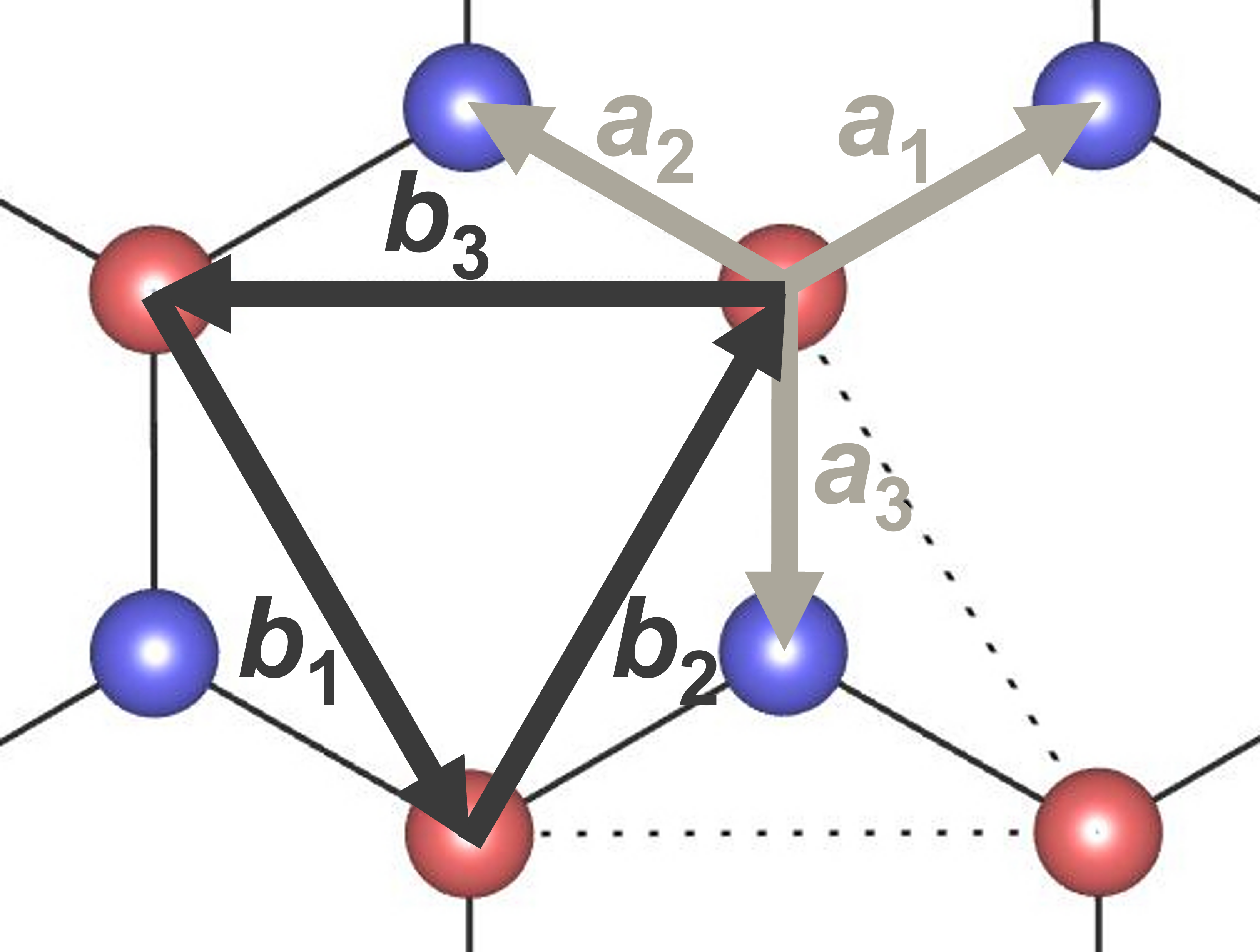
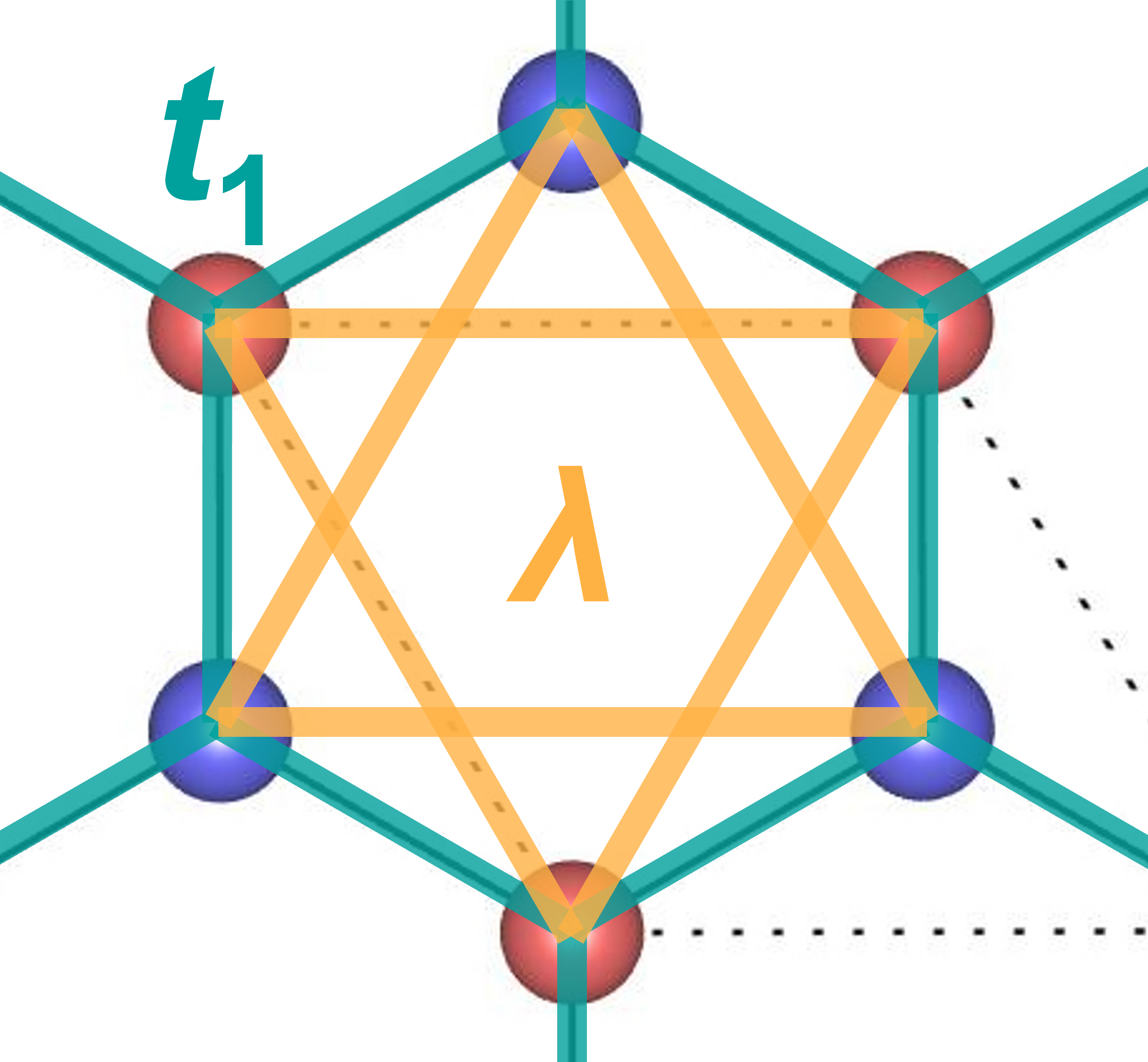
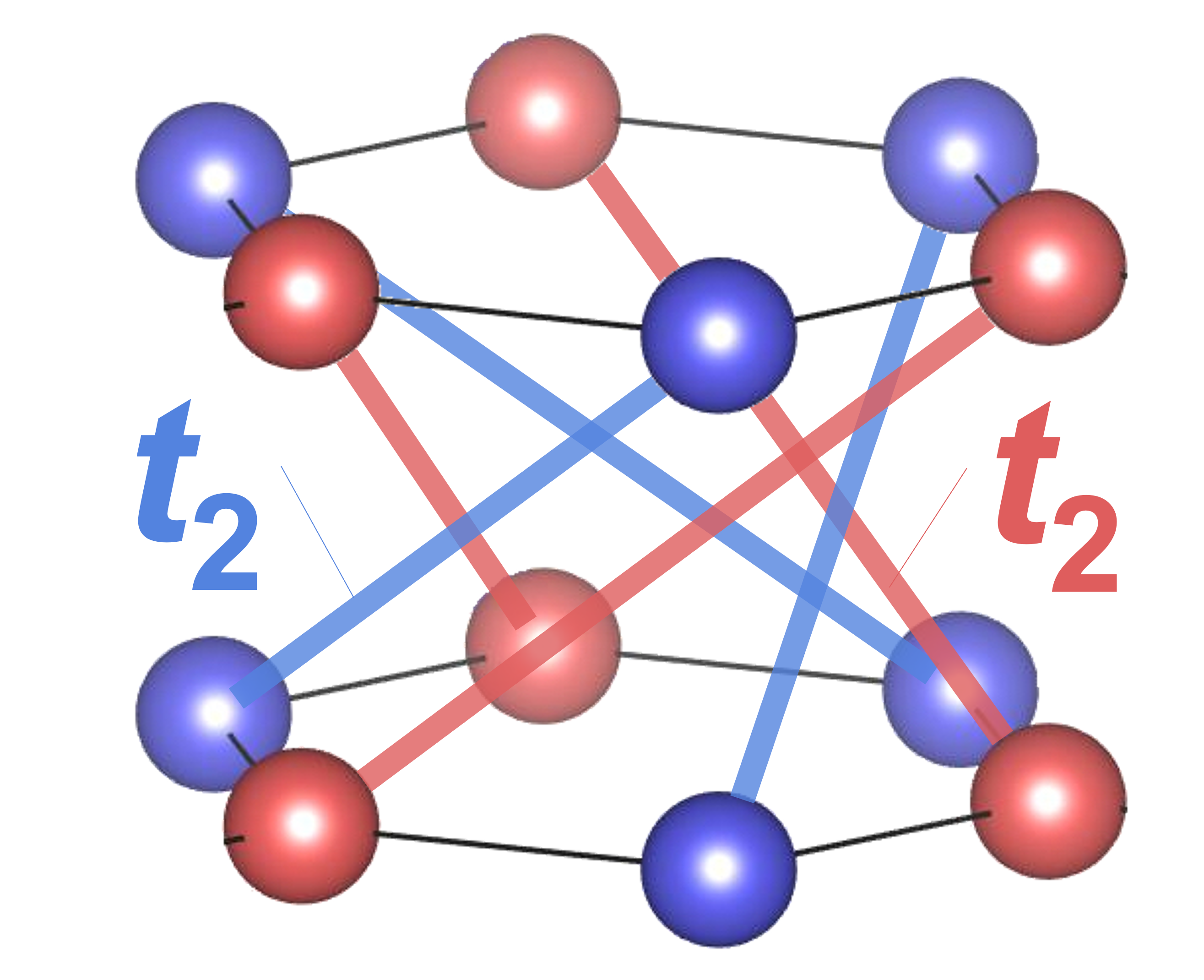
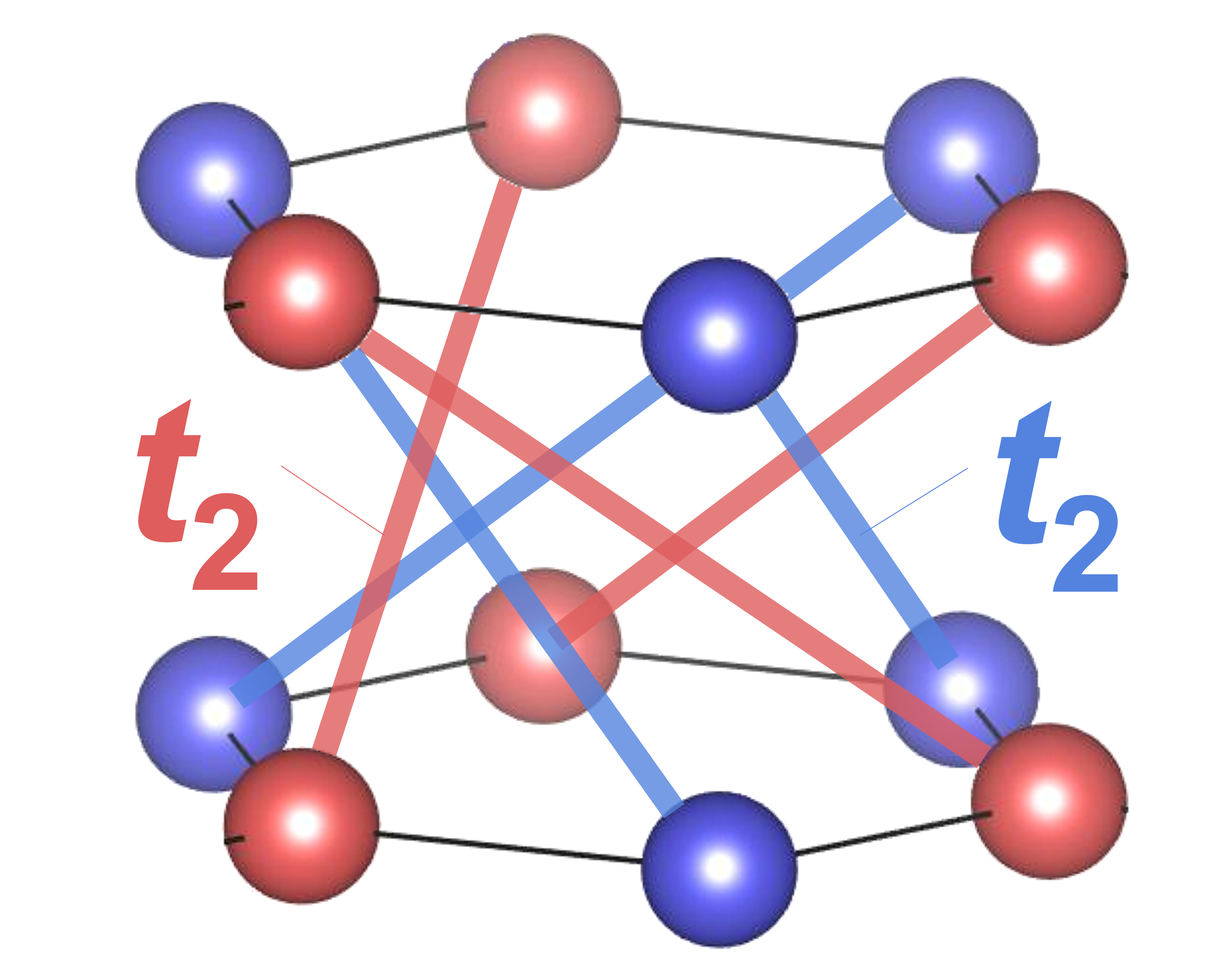
Figure 1: Tight-binding model described by the Hamiltonian in Eq. (9) [13]. 1 $xy$-plane of the present model. The vectors ${\bf\it a}_{a}$ and ${\bf\it b}_{a}$ ($a=1,2,3$) are shown in the figure. 1 Nearest-neighbor hopping (green) and next nearest-neighbor spin-orbit coupling (yellow) in the $xy$ plane. 11 Chiral hopping between the nearest-negihbor layers: 1 the right-handed model ($\chi=+1$) and 1 the left-handed model ($\chi=-1$).

The Hamiltonian in the wavenumber representation can be written as

$$\mathcal{H}({\bf\it k},s_{z},\chi) =d_{0}({\bf\it k})I+d_{x}({\bf\it k})\tau_{x}$$

$$+d_{y}({\bf\it k})\tau_{y}+d_{z}({\bf\it k},s_{z},\chi)\tau_{z},$$ (13)

$$d_{0}({\bf\it k}) =2t_{2}\sum_{a=1}^{3}\cos({\bf\it k}\cdot{\bf\it b}_{a})\cos(k_{z}c),$$ (14)

$$d_{x}({\bf\it k}) =t_{1}\sum_{a=1}^{3}\cos({\bf\it k}\cdot{\bf\it a}_{a}),$$ (15)

$$d_{y}({\bf\it k}) =t_{1}\sum_{a=1}^{3}\sin({\bf\it k}\cdot{\bf\it a}_{a}),$$ (16)

$$d_{z}({\bf\it k},s_{z},\chi) =-2\sum_{a=1}^{3}\sin({\bf\it k}\cdot{\bf\it b}_{a})(\chi t_{2}\sin(k_{z}c)+2s_{z}\lambda),$$ (17)

where $I$ is the identity matirx of size 2, ${\bf\it\tau}=(\tau_{x},\tau_{y},\tau_{z})$ are the Pauli matrices representing the sublattice degrees of freedom. The eigenenergies of the Hamiltonian in Eq. (13) are expressed as

$$\varepsilon_{\pm}({\bf\it k},s_{z},\chi)$$

$$= d_{0}({\bf\it k})\pm\sqrt{{d_{x}({\bf\it k})}^{2}+{d_{y}({\bf\it k})}^{2}+{d_{z}({\bf\it k},s_{z},\chi)}^{2}}.$$ (18)

The band structure of this model is shown in Fig. 2. Apparently, $\varepsilon_{\pm}({\bf\it k},s_{z},\chi)$ satisfies the time reversal condition in Eq. (6), and thus the relation in Eq. (7) holds, i.e., the first-order spin conductivity $\sigma^{\mathrm{s}}_{zz}$ vanishes.

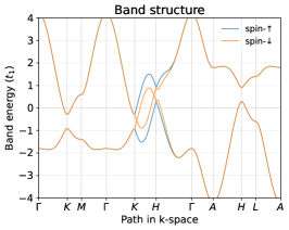
Figure 2: Band structure of the present model. The parameters are $t_{2}=0.2t_{1}$ and $\lambda=0.06t_{1}$.

To study the chirality dependence of the second-order spin conductivity $\sigma^{\mathrm{s}}_{zzz}(\chi)$, we study the dependence of $\varepsilon_{\pm}({\bf\it k},s_{z},\chi)$ on $\chi$. From Eq. (17), we obtain

$$d_{z}({\bf\it k},s_{z},\chi) =-d_{z}({\bf\it k},-s_{z},-\chi).$$ (19)

Then we can readily see that

$$\varepsilon_{\pm}({\bf\it k},s_{z},\chi) =\varepsilon_{\pm}({\bf\it k},-s_{z},-\chi),$$ (20)

$$\frac{\partial^{3}\varepsilon_{n}({\bf\it k},s_{z},\chi)}{{\partial k_{z}}^{3}} =-\frac{\partial^{3}\varepsilon_{n}({\bf\it k},-s_{z},-\chi)}{{\partial k_{z}}^{3}}.$$ (21)

Considering these equations with Eqs. (3) and (18), we obtain

$$\sigma_{zzz}(s_{z},\chi) =\sigma_{zzz}(-s_{z},-\chi).$$ (22)

Therefore, we can see

$$\sigma_{zzz}^{\mathrm{s}}(\chi) =-\sigma_{zzz}^{\mathrm{s}}(-\chi),$$ (23)

which means that the spin conductivity of the right-handed model $\sigma_{zzz}^{\mathrm{s}}(+1)$ and that of the left-handed model $\sigma_{zzz}^{\mathrm{s}}(-1)$ are of opposite signs in the present chiral tight-binding model.

In the following, we show that the chirality and the spin-orbit coupling of the present model play crucial roles in the chirality-dependent second-order spin current. Here we fix the chirality of the model $\chi$. When we assume that $t_{2}=0$, i.e., the model has no chirality, we obtain

$$\sigma_{zzz}(s_{z},\chi)=\sigma_{zzz}(-s_{z},\chi),$$ (24)

because $d_{z}({\bf\it k},s_{z},\chi)=-d_{z}({\bf\it k},-s_{z},\chi)$ holds as seen from Eq. (17). This means that the second-order spin conductivity $\sigma^{\mathrm{s}}_{zzz}(\chi)$ vanishes under $t_{2}=0$. Next, when we assume that $\lambda=0$, i.e., the model has no spin-orbit coupling, we obtain

$$\sigma_{zzz}(s_{z},\chi)=\sigma_{zzz}(-s_{z},\chi),$$ (25)

because $d_{z}({\bf\it k},s_{z},\chi)=d_{z}({\bf\it k},-s_{z},\chi)$ holds from Eq. (17). This means that the second-order spin conductivity $\sigma^{\mathrm{s}}_{zzz}(\chi)$ again vanishes under $\lambda=0$. From the above discussion, we can conclude that the chirality and the spin-orbit coupling are necessary for the chirality-dependent second-order spin current in the present model.

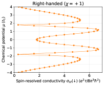
Figure 3: Calculated spin-resolved first-order conductivity. The parameters are $t_{2}=0.2t_{1}$ and $\lambda=0.06t_{1}$. The temperature $T$ is set at zero. 3 Spin-$\uparrow$ conductivity in the right-handed model. 3 Spin-$\downarrow$ conductivity in the right-handed model.

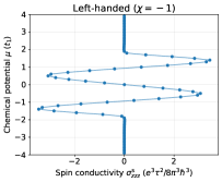
Figure 4: Calculated second-order spin conductivity. The parameters and temperature are the same as in Fig. 3. 4 Results for the right-handed model, and 4 for the left-handed model.

The calculated spin-resolved first-order conductivities and second-order spin conductivities are shown in Figs. 3 and 4. Figures 33 and 3 depict the chemical potential dependences of the spin-resolved first-order conductivities. The spin-$\uparrow$ conductivity has the same dependence as that of the spin-$\downarrow$ conductivity, which results in the zero spin conductivity in the first order with respect to the electric field, as discussed in Sect. II. Figures 44 and 4 depict the chemical potential dependences of the second-order spin conductivities. The spin conductivity in the left-handed model has the opposite sign as compared with that in the right-handed model, indicating that the sign of the spin conductivity can be controlled by reversing the chirality, as discussed above. Figure 4 shows that the second-order spin conductivity rapidly changes its sign depending on the chemical potential in the region of $-2<\mu/t_{1}<2$. This will originate from the difference in the energy dispersions of the spin-$\uparrow$ and spin-$\downarrow$ in the region of $-2<\varepsilon/t_{1}<2$ as shown in Fig. 2.

IV Conclusion

We explored the existence of spin current and its chirality dependence in systems with time-reversal symmetry. We evaluated the spin conductivity in the system with time-reversal symmetry based on the Boltzmann transport equation. We found that the first-order spin conductivity with respect to the electric field vanishes, while the second-order spin conductivity can be finite. We also evaluated the second-order spin conductivity using a specific chiral tight-binding model. As a result, we revealed the existence of the second-order spin conductivity depending on the chirality of the system. We also found that the chirality and the spin-orbit coupling play crucial roles in the chirality-dependent spin current.

We considered in this study the second-order spin conductivity with respect to the electric field because the first-order spin conductivity vanishes for the non-interacting single-channel systems with time-reversal symmetry [11]. However, spin polarization phenomena in the systems with spin hybridization have not been considered yet. The role of weak antisymmetric spin-orbit coupling in spin polarization phenomena is also discussed [7]. The mechanism in which the spin-flipping components of spin-orbit couplings affect the spin-polarized current remains to be investigated in future studies.

V Acknowledgement

This work was supported by Grants-in-Aid for Scientific Research from the Japan Society for the Promotion of Science (Grant No. JP18H01162), and by JST-Mirai Program (Grant No. JPMJMI19A1). R. H. was supported by Iwadare Scholarship Foundation and the Program for Leading Graduate Schools (MERIT-WINGS).

References

- Rikken et al. [2001] G. L. Rikken, J. Fölling, and P. Wyder, Phys. Rev. Lett. 87, 236602 (2001).
- Togawa et al. [2016] Y. Togawa, Y. Kousaka, K. Inoue, and J. I. Kishine, J. Phys. Soc. Jpn. 85, 1 (2016).
- Naaman and Waldeck [2012] R. Naaman and D. H. Waldeck, J. Phys. Chem. Lett. 3, 2178 (2012).
- Naaman and Waldeck [2015] R. Naaman and D. H. Waldeck, Annu. Rev. Phys. Chem. 66, 263 (2015).
- Göhler et al. [2011] B. Göhler, V. Hamelbeck, T. Z. Markus, M. Kettner, G. F. Hanne, Z. Vager, R. Naaman, and H. Zacharias, Science 331, 894 (2011).
- Xie et al. [2011] Z. Xie, T. Z. Markus, S. R. Cohen, Z. Vager, R. Gutierrez, and R. Naaman, Nano Lett. 11, 4652 (2011).
- Inui et al. [2020] A. Inui, R. Aoki, Y. Nishiue, K. Shiota, Y. Kousaka, H. Shishido, D. Hirobe, M. Suda, J. I. Ohe, J. I. Kishine, H. M. Yamamoto, and Y. Togawa, Phys. Rev. Lett. 124, 166602 (2020).
- Nabei et al. [2020] Y. Nabei, D. Hirobe, Y. Shimamoto, K. Shiota, A. Inui, Y. Kousaka, Y. Togawa, and H. M. Yamamoto, Appl. Phys. Lett. 117, 052408 (2020).
- Shishido et al. [2021] H. Shishido, R. Sakai, Y. Hosaka, and Y. Togawa, Appl. Phys. Lett. 119, 182403 (2021).
- Evers et al. [2022] F. Evers, A. Aharony, N. Bar-Gill, O. Entin-Wohlman, P. Hedegård, O. Hod, P. Jelinek, G. Kamieniarz, M. Lemeshko, K. Michaeli, V. Mujica, R. Naaman, Y. Paltiel, S. Refaely-Abramson, O. Tal, J. Thijssen, M. Thoss, J. M. van Ruitenbeek, L. Venkataraman, D. H. Waldeck, B. Yan, and L. Kronik, Adv. Mater. 2106629, 1 (2022).
- Bardarson [2008] J. H. Bardarson, J. Phys. A: Math. Theor. 41, 405203 (2008).
- Sodemann and Fu [2015] I. Sodemann and L. Fu, Phys. Rev. Lett. 115, 216806 (2015).
- Yoda et al. [2015] T. Yoda, T. Yokoyama, and S. Murakami, Sci. Rep. 5, 12024 (2015).