Quasinormal modes of self-dual black holes in loop quantum gravity

Abstract

We study the evolution of a test scalar field on the background geometry of a regular loop quantum black hole (LQBH) characterized by two loop quantum gravity (LQG) correction parameters, namely, the polymeric function and the minimum area gap. The calculations of quasinormal frequencies in asymptotically flat spacetime are performed with the help of higher-order WKB expansion and related Padé approximants, the improved asymptotic iteration method (AIM), and time-domain integration. The effects of free parameters of the theory on the quasinormal modes are studied and deviations from those of the Schwarzschild BHs are investigated. We show that the LQG correction parameters have opposite effects on the quasinormal frequencies and the LQBHs are dynamically stable.

I Introduction

The quasinormal modes (QNMs) are the intrinsic imprints of BH response to external perturbations on its background geometry Kokkotas ; BertiR ; KonoplyaR . The QNMs spectrum is an essential characteristic of BHs that depends on BH charges and could be detected through the gravitational wave interferometers Abbott2016 ; Abbott2017 ; Isi . Hence, this capability allows us to explore the properties of background spacetime of BHs, check the validity of the alternative theories of general relativity, and estimate the BH parameters by studying gravitational waves (GWs) at the ringdown stage GWspectroscopy ; RoadMap .

Furthermore, some other potent motivations for investigating the QN oscillations of BHs in different branches of fundamental physics can be listed as follows. The QNMs spectrum governs the dynamic stability of BHs undergoing small perturbations of various test fields Kokkotas ; BertiR ; KonoplyaR , the asymptotic behavior of the QN modes in the flat background plays a crucial role in the semi-classical approach to quantum gravity Hod , the highly damped QN frequencies used to fix the so-called Barbero-Immirzi parameter appearing in LQG Dreyer , the imaginary part of the QN frequencies in asymptotically anti-de Sitter spacetime describes the decay of perturbations of corresponding thermal state in the conformal field theory Horowitz ; LemosAdS ; KokkotasAdS ; MehrabJHEP ; MehrabSultani , and the correspondence between the QN frequencies in the eikonal limit and unstable circular null geodesics that describe the size of the BH shadow CardosoUCNG ; KonoplyaUCNG ; MomenniaPRD .

On the other hand, scalar fields have been considered extensively as candidates for dark energy Gubitosi and dark matter Hu . They have been also investigated as the inflatons in the context of cosmology Cheung . Background scalar fields are a generic feature in the string theory Metsaev ; Arvanitaki , and they have been used to modify the background spacetime of BHs in the strong-field regime Herdeiro ; Silva . Besides, the scalar fields produce scalar clouds around BHs through superradiant instability Brito .

In gravitational models non-minimally coupled to scalar fields, the emitted GWs is a linear combination of GWs in the gravitational theory and the scalar field solutions Tattersall . Thus, the gravitational waves $\bar{h}_{\mu\nu}$ that could potentially be observed, will be a linear combination of GWs in the gravitational theory, $h_{\mu\nu}$, and the scalar field solutions of the form

$$\bar{h}_{\mu\nu}=h_{\mu\nu}+\beta g_{\mu\nu}\Phi,$$ (1)

where $\Phi$ is the scalar field, $g_{\mu\nu}$ is the background metric, and $\beta$ is an arbitrary function of the scalar field that characterizes the non-minimal coupling. However, the interaction of spacetime metric and scalar waves depends on the scalar propagation speed so that interactions are negligible for luminal scalar waves Dalang .

The scalar fields minimally coupled to gravity describe the QNMs in the context of scalar-tensor theories. More recently, it has been demonstrated that the Laser Interferometer Space Antenna will be able to measure the scalar charge with an accuracy of the order of percent in the extreme mass ratio inspirals Maselli . This analysis indicated that the detectability of the scalar charge does not depend on the scalar field origin and the structure of the secondary compact object that is coupled to the scalar field.

In the extended and modified gravity theories of general relativity, the QNMs of BH solutions undergoing scalar perturbations have been investigated in higher dimensional Einstein-Yang-Mills theory YangMills , Einstein-Born-Infeld gravity BornInfeld , dRGT massive gravity dRGT , conformal Weyl gravity MehrabSultani ; MomenniaPRD , and loop quantum gravity QNMofLQG . In addition, the QN modes of Schwarzschild BHs with Robin boundary conditions Robin , the dirty BHs Dirty , the Kaluza–Klein BHs KKBH , and charged BHs with Weyl corrections Weylcorrections have been studied.

When it comes to BH physics, the intrinsic singularity inside the event horizon has a special place. Although the properties of spacetime outside the event horizon are described by a few parameters characterizing the BH conserved charges, the curvature singularity at the center of BHs remained a crucial and outstanding problem. In this context, people have performed plenty of efforts to address this issue, such as assigning conformal symmetry to spacetime, employing nonlinear electrodynamic fields, and considering quantum corrections to general relativistic theories. However, we expect a too strong bending of the spacetime near the BH center such that the general relativity breaks down and a quantum description of gravity becomes inevitable.

In this paper, we focus on scalar perturbations in the background spacetime of a non-singular LQBH to investigate the effects of the LQG correction parameters on the scalar QNM spectrum, explore the dynamical stability of the BHs, and find deviations from those of the Schwarzschild solutions. Our regular BH case study, also known as the self-dual BH, was constructed in the mini-superspace approach based on the polymerization procedure in LQG LQBH  and characterized by the polymeric function and the minimum area gap as two LQG correction parameters (see Perez ; Barrau  for review papers on BHs in LQG and EHDestruction for the role of quantum corrections on the destruction of the event horizon). Particle creation by these LQBHs is investigated and it was shown that the evaporation time is infinite ParticleCreation . The gravitational lensing by the LQBHs in the strong and weak deflection regimes is studied Lensing . These quantum-corrected BHs were generalized to axially symmetric spacetimes and their shadow is investigated LQBHJamil . However, the QNMs of the static case have been calculated with some defects in LQBHJamil ; Chen2011 ; BarrauUniverse , and we shall address this issue in the present study as well.

The outline of this paper is as follows. Section II is devoted to a brief review of LQG-corrected BHs and perturbation equations of a test scalar field. Then, we briefly explain the higher-order WKB approximation and related Padé approximants, the improved AIM, and the time-domain integration that are used to investigate the QN modes. In Sec. III, we calculate the QNMs of LQBHs, study the effects of LQG correction parameters on the QNMs spectrum, and find deviations from those of the Schwarzschild BHs. Besides, we investigate the dynamical stability of the LQBHs, and compute the QNMs by employing the higher-order WKB formula and related Padé approximants as a semi-analytic method. We finish our paper with some concluding remarks.

II Loop Quantum Black holes and perturbation equations

The effective LQG-corrected line element, also known as the self-dual spacetime, with spherical symmetry that is geodesically complete is given by LQBH

$$ds^{2}=-f(r)dt^{2}+\frac{dr^{2}}{g(r)}+h(r)d\Omega^{2},$$ (2)

where $d\Omega^{2}$ is the line element of a $2$-sphere and the metric functions $f(r)$, $g(r)$, and $h(r)$ can be written as

$$f(r)=\frac{\left(r-r_{+}\right)\left(r-r_{-}\right)}{r^{4}+A_{0}^{2}}\left(r+r_{0}\right)^{2},$$ (3)

$$g(r)=\frac{\left(r-r_{+}\right)\left(r-r_{-}\right)}{r^{4}+A_{0}^{2}}\frac{r^{4}}{\left(r+r_{0}\right)^{2}},$$ (4)

$$h(r)=r^{2}+\frac{A_{0}^{2}}{r^{2}},$$ (5)

with the outer (event) horizon $r_{+}=2M/(1+P)^{2}$, the inner (Cauchy) horizon $r_{-}=2MP^{2}/(1+P)^{2}$, and the polymeric function $P=\left(\sqrt{1+\epsilon^{2}}-1\right)/\left(\sqrt{1+\epsilon^{2}}+1\right)$ arising from the geometric quantum effects of LQG. Besides, $A_{0}$ is related to the minimum area gap of LQG as $A_{0}=A_{\min}/(8\pi)$ and $r_{0}=\sqrt{r_{+}r_{-}}=2MP/(1+P)^{2}$. In the aforementioned relations, $M$ is the total mass of the BHs, and $\epsilon$ denotes a product of the Immirzi parameter $\gamma$ and the polymeric parameter $\delta$ satisfying $\epsilon=\gamma\delta<<1$.

It is worthwhile to mention that the inner horizon is produced due to LQG generalization, and these BHs reduce to a single-horizon BH whenever the polymeric function $P$ vanishes (see Fig. 1). Besides, note that the LQG correction parameters $\epsilon$ and $A_{0}$ describe deviations from the Schwarzschild solutions. Therefore, the LQBHs (2) reduce to Schwarzschild BHs by taking the limit $\epsilon=0=A_{0}$.

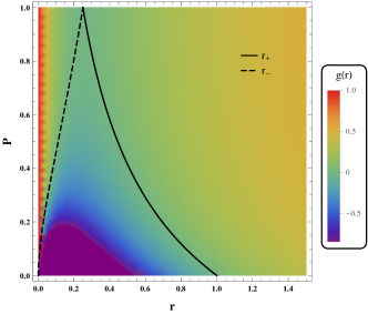
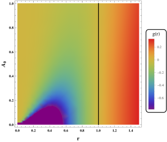
Figure 1: The metric function $g(r)$ in $r-P$ plane for $A_{0}=0$ (left panel) and $r-A_{0}$ plane for $P=0$ (right panel). The non-zero values of the polymeric function produce an inner horizon and decrease the event horizon radius (see the left panel). The vertical black line in the right panel denotes the event horizon radius $r_{+}$ of the single-horizon BH.

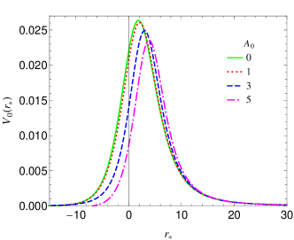
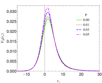
Figure 2: The effective potential versus tortoise coordinate for $M=1$, $l=0$, $P=0$ (left panel), and $A_{0}=0$ (right panel). The continuous green curve denotes the Schwarzschild’s potential. The potential forms a barrier and vanishes at both infinities (in order to see the effects of $A_{0}$ on the potential, large values were adopted).

Now, we consider a scalar perturbation in the background of the LQBHs to investigate their QNMs spectrum. The equation of motion for a minimally coupled scalar field is given by

$$\nabla_{\mu}\nabla^{\mu}\Phi\left(t,r,\theta,\varphi\right)=0.$$ (6)

The following expansion of modes

$$\Phi\left(t,r,\theta,\varphi\right)=\int d\omega e^{-i\omega t}\sum_{l,m}\frac{1}{\sqrt{h(r)}}\Psi_{l}\left(r\right)Y_{l,m}\left(\theta,\varphi\right),$$ (7)

allows us to find a Schrödinger-like wave equation for the radial part $\Psi_{l}\left(r\right)$ of perturbations, and $Y_{l,m}\left(\theta,\varphi\right)$ denotes the spherical harmonics on a $2$-sphere. Substituting the decomposition (7) into the Klein–Gordon equation (6), the equation of motion reduces to the following wave-like equation for the radial part of the perturbations

$$\left[\partial_{r_{\ast}}^{2}+\omega^{2}-V_{l}\left(r_{\ast}\right)\right]\Psi_{l}\left(r_{\ast}\right)=0,$$ (8)

where $\omega$ is the Fourier variable presented in Eq. (7). In this relation, $V_{l}\left(r_{\ast}\right)$ is the effective potential that is given by

$$V_{l}\left(r_{\ast}\right) = f\left(r\right)\frac{l\left(l+1\right)}{h(r)}$$ (9)

$$+\sqrt{\frac{f(r)g(r)}{h(r)}}\partial_{r}\left(\sqrt{f(r)g(r)}\partial_{r}\sqrt{h(r)}\right),$$

where $l$ is the angular quantum (multipole) number, and$\ r_{\ast}$ is the tortoise coordinate with the following explicit form

$$r_{\ast} = \int\frac{dr}{\sqrt{f(r)g(r)}}=r-\frac{A_{0}^{2}}{r_{+}r_{-}}\left(\frac{1}{r}-\frac{r_{+}+r_{-}}{r_{+}r_{-}}\ln\left(r\right)\right)$$ (10)

$$+\frac{1}{\left(r_{+}-r_{-}\right)}\left(\frac{A_{0}^{2}+r_{+}^{4}}{r_{+}^{2}}\ln\left(r-r_{+}\right)\right.$$

$$\left.-\frac{A_{0}^{2}+r_{-}^{4}}{r_{-}^{2}}\ln\left(r-r_{-}\right)\right),$$

that ranges from $-\infty$ at the event horizon to $+\infty$ at spatial infinity, and note that $r$ in the right-hand side of (9) is a function of $r_{\ast}$ by (10). Figure 2 shows the behavior of the effective potential (9) versus the tortoise coordinate for different values of the LQBH parameters $P$ and $A_{0}$. From this figure, we find that the effect of $P$ on the effective potential is much more than the minimum area gap $A_{0}$, and therefore it plays a more important role in the context of LQBH oscillations.

The spectrum of QN modes is a solution to the wave equation (8) and we should impose some physically motivated boundary conditions at the boundaries to find the solutions. The quasinormal boundary conditions imply that the wave at the event horizon is purely incoming and it is purely outgoing at spatial infinity, such that

$$\left\{\begin{array}[]{c}\Psi_{l}\left(r_{\ast}\right)\sim e^{-i\omega r_{\ast}}\ \ \ as\ \ \ r_{\ast}\rightarrow-\infty\ (r\rightarrow r_{+}),\\ \Psi_{l}\left(r_{\ast}\right)\sim e^{i\omega r_{\ast}}\ \ \ \ as\ \ \ \ \ \ r_{\ast}\rightarrow\infty\ (r\rightarrow\infty),\end{array}\right..$$ (11)

These boundary conditions lead to a discrete set of eigenvalues $\omega_{nl}=\omega_{r}-i\omega_{i}$ with a real part giving the actual oscillation and an imaginary part representing the damping of the perturbation. The indices of $\omega_{nl}$ denote the overtone number $n$ and multipole number $l$. In this paper, we investigate the QN modes of LQBHs by using a couple of independent computational methods, such as the higher-order Wentzel–Kramers–Brillouin (WKB) approximation and related Padé approximants, the improved AIM, and the time-domain integration that we briefly explain in the following subsections.

II.1 WKB approximation

The WKB approximation is based on the matching of WKB expansion of the modes $\Psi_{l}\left(r_{\ast}\right)$ at the event horizon and spatial infinity with the Taylor expansion near the peak of the potential barrier through two closely spaced turning points characterized by $\omega^{2}-V_{l}\left(r_{\ast}\right)=0$. Therefore, the WKB method can be used for an effective potential that forms a potential barrier and takes zero values (or small values compared with the height of the barrier) at the event horizon ($r_{\ast}\rightarrow-\infty$) and spatial infinity ($r_{\ast}\rightarrow+\infty$).

This method first applied to the problem of scattering around BHs Schutz , and is extended to the $3$rd IyerWill , $6$th order Konoplya6th , and $13$th order Matyjasek13th . The $13$th order of WKB approximation is given by the following formula

$$\omega^{2}=V_{0}+\sum_{j=1}^{6}\Omega_{2j}-i\sqrt{-2V_{0}^{\prime\prime}}\left(n+\frac{1}{2}\right)\times$$

$$\left(1+\sum_{j=1}^{6}\Omega_{2j+1}\right);\ \ \ \ n=0,1,2,...,$$ (12)

where $V_{0}$ denotes the height of the effective potential, $\Omega_{j}$’s are the WKB correction terms of the $j$th order that depend on the value of the effective potential and its derivatives at the local maximum, and $n$ is the overtone number.

It is worthwhile to mention that the WKB formula does not give reliable frequencies for $n\geq l$, while it leads to accurate values for $n<l$  and exact modes in the eikonal limit $l\rightarrow\infty$. We use this formula up to the $13$th order to calculate the QN frequencies of perturbations.

On the other hand, one can use Padé approximants for the WKB formula (12) to increase the accuracy of this method Matyjasek13th . In order to incorporate the Padé approximants, we first define a polynomial $\mathcal{P}_{k}\left(\varepsilon\right)$ by multiplying the powers of the order parameter $\varepsilon$ in the WKB correction terms as below KonoplyaPade

$$\mathcal{P}_{k}\left(\varepsilon\right) = V_{0}+\sum_{j=1}^{6}\varepsilon^{2j}\Omega_{2j}-i\sqrt{-2V_{0}^{\prime\prime}}\left(n+\frac{1}{2}\right)\times$$ (13)

$$\left(\varepsilon+\sum_{j=1}^{6}\varepsilon^{2j+1}\Omega_{2j+1}\right),$$

such that the polynomial order $k$ coincides with the WKB order and the squared frequency can be obtained by setting $\varepsilon=1$ as $\omega^{2}=\mathcal{P}_{k}\left(1\right)$. Then, we introduce a class of the Padé approximants $\mathcal{P}_{\tilde{n}/\tilde{m}}\left(\varepsilon\right)$ of the polynomial $\mathcal{P}_{k}\left(\varepsilon\right)$ near $\varepsilon=0$ with the condition $k=\tilde{n}+\tilde{m}$ to obtain

$$\mathcal{P}_{\tilde{n}/\tilde{m}}\left(\varepsilon\right)=\left(\sum\limits_{i=0}^{\tilde{n}}Q_{i}\varepsilon^{i}\right)\left/\left(\sum\limits_{i=0}^{\tilde{m}}R_{i}\varepsilon^{i}\right)\right.,$$ (14)

with

$$\mathcal{P}_{\tilde{n}/\tilde{m}}\left(\varepsilon\right)-\mathcal{P}_{k}\left(\varepsilon\right)=\mathcal{O}\left(\varepsilon^{k+1}\right).$$ (15)

As the next step, since the right-hand side of the WKB formula (12) is known, we can calculate the coefficients $Q_{i}$’s and $R_{i}$’s of (14) numerically and employ the rational function $\mathcal{P}_{\tilde{n}/\tilde{m}}\left(\varepsilon\right)$ to approximate the squared frequency as $\omega^{2}=\mathcal{P}_{\tilde{n}/\tilde{m}}\left(1\right)$.

In most cases, the Padé approximation (14) of the order $k=\tilde{n}+\tilde{m}$ gives more accurate results for $\tilde{n}\approx\tilde{m}$ compared to the ordinary WKB formula (12) of the same order KonoplyaPade . However, there is no way to choose the appropriate orders $\tilde{n}$ and $\tilde{m}$ to obtain the frequency with the highest accuracy. In order to find the suitable orders $\tilde{n}$ and $\tilde{m}$, we follow an approach based on averaging of Padé approximations suggested in KonoplyaPade so that the minimum of the standard deviation (SD) formula supposed to specify the most accurate modes.

II.2 Asymptotic iteration method

The AIM has been employed to solve the eigenvalue problems and second-order differential equations Ciftci ; CiftciHall , and then it was indicated that an improved version of AIM is an accurate technique for calculating QN modes Naylor ; AIM ; MomenniaPRD .

Here, we consider the effect of the LQG correction parameters $P$ and $A_{0}$ separately to investigate the contribution of either parameter on the QNMs spectrum and find deviations from those of the Schwarzschild BHs. Thus, we study the QNMs for different values of one LQG correction parameter while setting the other one equals to zero. To do so, consider two cases as follows; one is the $P=0$ case that leads to a single-horizon LQBH with $r_{+}=2M$, and the second case is given by $A_{0}=0$ which represents LQBHs with two distinct horizons.

II.2.1 $P=0$ case

First, note that the wave equation (8) has the following form in the $r$-coordinate

$$f^{2}(r)\Psi^{\prime\prime}(r)+f(r)f^{\prime}(r)\Psi^{\prime}(r)+\left[\omega^{2}-V(r)\right]\Psi(r)=0,$$ (16)

where prime denotes the derivative with respect to $r$ and we used the fact that $g(r)=f(r)$. Equation (16) is a second-order ordinary differential equation with two regular singular points located at $r=0$ and $r=r_{+}$. In order to apply the boundary conditions (11) to this differential equation, we follow Leaver LeaverSchw and define the following solution

$$\Psi(r) = e^{i\omega\left(r-r_{+}\right)}\left(\frac{r}{r_{+}}\right)^{i\omega r_{+}}{}\times$$ (17)

$$\left(\frac{r-r_{+}}{r}\right){}^{-i\omega\left(A_{0}^{2}+r_{+}^{4}\right)/r_{+}^{3}}\psi\left(r\right),$$

which has the correct asymptotic behavior at the boundaries and $\psi\left(r\right)$ is a finite and convergent function. Since the AIM works better on a compact domain, we also define a new variable $\xi=1-r_{+}/r$. Thus, $\xi$ ranges $0\leq\xi<1$ so that $\xi\approx 1$ represents the spatial infinity and $\xi_{+}=0$ corresponds to the event horizon.

Now, by considering the new variable $\xi$ and the solution (17), we can find the standard AIM form of the wave equation (16) as follows

$$\psi^{\prime\prime}(\xi)=\lambda_{0}\left(\xi\right)\psi^{\prime}(\xi)+s_{0}\left(\xi\right)\psi(\xi),$$ (18)

where prime denotes the derivative with respect to $\xi$, and $\lambda_{0}\left(\xi\right)$ and $s_{0}\left(\xi\right)$ are

$$\lambda_{0}\left(\xi\right) = \frac{2}{1-\xi}-\frac{A_{0}^{2}(1-\xi)^{3}(3\xi+1)+r_{+}^{4}}{\xi z}+\frac{2i\omega y}{\xi r_{+}^{3}(1-\xi)^{2}},$$ (19)

$$s_{0}\left(\xi\right) = \frac{1}{(1-\xi)^{4}\xi^{2}r_{+}^{4}}\left\{\frac{i\omega r_{+}(1-\xi)^{2}\left[r_{+}^{4}+A_{0}^{2}(1-\xi)^{3}(3\xi+1)\right]y}{z}\right.$$ (20)

$$+\frac{\xi r_{+}^{4}(1-\xi)^{2}}{z^{2}}\left(l(l+1)z^{2}+r_{+}^{8}(1-\xi)+A_{0}^{2}(1-\xi)^{8}\left[\frac{10\xi r_{+}^{4}}{(1-\xi)^{4}}-A_{0}^{2}(1+\xi)\right]\right)$$

$$\left.+\frac{\omega^{2}}{r_{+}^{2}}\left(y^{2}-z^{2}\right)-2i\omega\xi r_{+}(1-\xi)y-i\omega r_{+}\left(z+\xi r_{+}^{4}\left[2\xi^{2}(\xi-4)+9\xi-4\right]\right)\right\},$$

with $y=2\xi r_{+}^{4}(\xi-2)+r_{+}^{4}+A_{0}^{2}(1-\xi)^{2}$ and $z=r_{+}^{4}+A_{0}^{2}(1-\xi)^{4}$.

II.2.2 $A_{0}=0$ case

On the other hand, as for the $P=0$ case, we also obtain the standard AIM form of the wave equation for $A_{0}=0$. The wave equation (8) has the following form in the $r$-coordinate

$$f(r)g(r)\Psi^{\prime\prime}(r)+\partial_{r}\left[\sqrt{f(r)g(r)}\right]\sqrt{f(r)g(r)}\Psi^{\prime}(r)$$

$$+\left[\omega^{2}-V(r)\right]\Psi(r)=0.$$ (21)

In this case, we deal with BHs with two horizons located at $r_{-}$ and $r_{+}$, and therefore the differential equation (21) contains three regular singular points located at $r=0$, $r=r_{-}$, and $r=r_{+}$. Following LeaverRN , we define the solution

$$\Psi(r) = e^{i\omega r}r^{-1}\left(r-r_{-}\right){}^{1+i\omega r_{+}+i\omega r_{+}^{2}/\left(r_{+}-r_{-}\right)}\times$$ (22)

$$\left(r-r_{+}\right){}^{-i\omega r_{+}^{2}/\left(r_{+}-r_{-}\right)}\psi(r),$$

to apply the boundary conditions (11) such that $\psi\left(r\right)$ is a finite and convergent function. One may note that the solutions (17) and (22) are not consistent in the common limit $A_{0}=0=P$. In this regard, we should mention that the constant $e^{-i\omega r_{+}}r_{+}^{-i\omega r_{+}}$ was multiplied to the solution (17) by hand to obtain a simpler form for the relations (19) and (20).

Now, we can find the standard AIM form of the wave equation (21) with the help of the new variable $\xi$ and the solution (22) as below

$$\psi^{\prime\prime}(\xi)=\hat{\lambda}_{0}\left(\xi\right)\psi^{\prime}(\xi)+\hat{s}_{0}\left(\xi\right)\psi(\xi),$$ (23)

where $\hat{\lambda}_{0}\left(\xi\right)$ and $\hat{s}_{0}\left(\xi\right)$ are

$$\hat{\lambda}_{0}\left(\xi\right) = \frac{r_{+}\left[2i\omega r_{+}\left(2\xi^{2}-4\xi+1\right)-3\xi^{2}+4\xi-1\right]+r_{-}(1-\xi)\left[1+\xi\left(2i\omega r_{+}+6\xi-7\right)\right]}{\xi(1-\xi)^{2}\left[r_{+}-r_{-}(1-\xi)\right]},$$ (24)

$$\hat{s}_{0}\left(\xi\right) = \frac{1}{\xi^{2}(1-\xi)^{4}\left[r_{+}-(1-\xi)r_{-}\right]^{2}}\left[r_{+}^{4}V(\xi)-\xi(1-\xi)\times\right.$$ (25)

$$\left\{r_{-}(1-\xi)^{2}\left[r_{+}(1-3\xi)-r_{-}(1-\xi)(1-4\xi)\right]\right.$$

$$+i\omega r_{+}(1-\xi)\left[4r_{+}^{2}(1-\xi)-r_{+}r_{-}\left(8\xi^{2}-18\xi+7\right)+r_{-}^{2}(1-\xi)(1-4\xi)\right]$$

$$\left.\left.-r_{+}^{2}\omega^{2}\left[r_{-}\left(1-\xi\right)-2r_{+}(2-\xi)\right]\left[r_{-}\xi+2r_{+}(1-\xi)\right]\right\}\right].$$

Once the standard AIM form of the master wave equation is obtained in (18) and (23), we can express higher derivatives of $\psi\left(\xi\right)$ in terms of $\psi\left(\xi\right)$ and $\psi^{\prime}\left(\xi\right)$ as follows

$$\psi^{(n+2)}\left(\xi\right)=\lambda_{n}\left(\xi\right)\psi^{\prime}\left(\xi\right)+s_{n}\left(\xi\right)\psi\left(\xi\right),$$ (26)

with the recurrence relations

$$\begin{array}[]{c}\lambda_{n}\left(\xi\right)=\lambda_{n-1}^{\prime}\left(\xi\right)+s_{n-1}\left(\xi\right)+\lambda_{0}\left(\xi\right)\lambda_{n-1}\left(\xi\right),\\ \\ s_{n}\left(\xi\right)=s_{n-1}^{\prime}\left(\xi\right)+s_{0}\left(\xi\right)\lambda_{n-1}\left(\xi\right).\end{array}$$ (27)

We now expand $\lambda_{n}\left(\xi\right)$ and $s_{n}\left(\xi\right)$ in a Taylor series around some point $\bar{\xi}$ at which the AIM is performed

$$\begin{array}[]{c}\lambda_{n}\left(\xi\right)=\sum\limits_{j=0}^{\infty}c_{n}^{j}\left(\xi-\bar{\xi}\right)^{j},\\ \\ s_{n}\left(\xi\right)=\sum\limits_{j=0}^{\infty}d_{n}^{j}\left(\xi-\bar{\xi}\right)^{j},\end{array}$$ (28)

which allows us to rewrite the recurrence relations (27) in terms of the series coefficients $c_{n}^{j}$ and $d_{n}^{j}$

$$c_{n}^{j}=\left(j+1\right)c_{n-1}^{j+1}+d_{n-1}^{j}+\sum\limits_{k=0}^{j}c_{0}^{k}c_{n-1}^{j-k},$$ (29)

$$d_{n}^{j}=\left(j+1\right)d_{n-1}^{j+1}+\sum\limits_{k=0}^{j}d_{0}^{k}c_{n-1}^{j-k}.$$ (30)

For sufficiently large $n$, we consider the following termination to the number of iterations

$$\frac{s_{n}\left(\xi\right)}{\lambda_{n}\left(\xi\right)}=\frac{s_{n-1}\left(\xi\right)}{\lambda_{n-1}\left(\xi\right)},$$ (31)

which leads to

$$\delta_{n}=s_{n}\left(\xi\right)\lambda_{n-1}\left(\xi\right)-s_{n-1}\left(\xi\right)\lambda_{n}\left(\xi\right)=0,$$ (32)

and in terms of the Taylor series coefficients, we have

$$d_{n}^{0}c_{n-1}^{0}-d_{n-1}^{0}c_{n}^{0}=0,$$ (33)

that is known as the quantization condition and gives an equation in terms of the QN frequencies $\omega$. As the next step, we fix all the free parameters, namely, the multipole number $l$, the BH mass $M$, the polymeric function $P$, and the minimum area gap of LQG $A_{0}$. Finally, we use the quantization condition (33) and a root finder to calculate the QN modes.

II.3 Ringdown waveform

In order to investigate the contribution of all modes, we can integrate the wave-like equation (8) on a finite time domain. This also helps us to explore the time evolution of modes and dynamical stability of the BH case study. To do so, we follow Gundlach  and write the perturbation equation (8) in terms of the light-cone coordinates $u=t-r_{\ast}$ and $v=t+r_{\ast}$ in the following form

$$-4\frac{\partial^{2}\Psi_{l}\left(u,v\right)}{\partial u\partial v}=V_{l}\left(u,v\right)\Psi_{l}\left(u,v\right),$$ (34)

where $\Psi_{l}$ assumed to have time dependence $e^{-i\omega t}$. To find a unique solution to (34), the initial data must be specified on the two null surfaces $u=u_{0}$ and $v=v_{0}$. Here, we set $\Psi_{l}\left(u,0\right)=1$ at $v=0$, and use the Gaussian wave packet

$$\Psi_{l}\left(0,v\right)=\exp\left(-\frac{\left(v-v_{c}\right)^{2}}{2\sigma^{2}}\right),$$ (35)

centered on $v_{c}$ and having width $\sigma$ at $u=0$. Then, we choose the observer to be located at $r=5r_{+}$ and use built-in Wolfram Mathematica commands for solving partial differential equations to generate the ringdown waveforms. Finally, we employ the Prony method Marple ; Prony , a method for mining information from (damped) sinusoidal signals, to extract dominant (fundamental) frequency from the data generated in the ringdown profile.

III Quasinormal Modes

Before investigating the QN oscillations by using the mentioned methods in general, let us first reconstruct Tables I and II of LQBHJamil  by employing the $6$th order WKB approximation. We present our results in Tables 1 and 2 with the relative error $\left|\left(\mathring{\omega}-\omega\right)/\omega\right|\times 100\%$, where $\mathring{\omega}$’s are given in LQBHJamil  through Tables I and II, and $\omega$’s are presented in our Tables 1 and 2. Although both $\mathring{\omega}$ and $\omega$ were calculated by employing the $6$th order WKB formula, our tables indicate a disagreement between $\mathring{\omega}$ and $\omega$. The error increases as the polymeric function increases and it is about $30\%$ in the worst case. We found that the WKB method was not properly used which led to this error (see KonoplyaPade to find popular mistakes when employing the WKB approximation). Therefore, figures $9$ and $10$ illustrated in LQBHJamil  should be modified according to the following tables as well.

$P$		$\omega_{01}$	$\omega_{02}$	$\omega_{12}$
$0.0$		$0.2929-0.0978i(0.00\%)$	$0.4836-0.0968i(0.00\%)$	$0.4638-0.2956i(0.00\%)$
$0.1$		$0.3739-0.1192i(4.62\%)$	$0.6206-0.1184i(2.71\%)$	$0.5987-0.3612i(7.82\%)$
$0.2$		$0.4652-0.1405i(9.07\%)$	$0.7757-0.1400i(5.35\%)$	$0.7528-0.4260i(15.6\%)$
$0.3$		$0.5653-0.1603i(13.1\%)$	$0.9463-0.1600i(7.82\%)$	$0.9236-0.4860i(23.1\%)$
$0.4$		$0.6717-0.1770i(16.7\%)$	$1.1280-0.1771i(9.99\%)$	$1.1067-0.5366i(29.8\%)$

Table 1: The QNMs $\omega_{nl}$ of scalar perturbations for $M=1$ and $A_{0}=0.01$ calculated by the $6$th order WKB formula.

$P$		$\omega_{01}$	$\omega_{02}$	$\omega_{12}$
$0.0$		$0.2482-0.0926i(0.00\%)$	$0.4576-0.0950i(0.00\%)$	$0.4365-0.2907i(0.00\%)$
$0.1$		$0.3226-0.1141i(4.90\%)$	$0.5908-0.1167i(2.77\%)$	$0.5676-0.3562i(8.03\%)$
$0.2$		$0.4084-0.1357i(9.58\%)$	$0.7426-0.1383i(5.48\%)$	$0.7184-0.4214i(16.0\%)$
$0.3$		$0.5043-0.1560i(13.9\%)$	$0.9108-0.1586i(7.99\%)$	$0.8869-0.4820i(23.7\%)$
$0.4$		$0.6082-0.1734i(17.8\%)$	$1.0911-0.1759i(10.2\%)$	$1.0686-0.5334i(30.5\%)$

Table 2: The QNMs $\omega_{nl}$ of electromagnetic perturbations for $M=1$ and $A_{0}=0.01$ calculated by the $6$th order WKB formula.

$A_{0}$		$\omega_{00}$	$\omega_{01}$	$\omega_{02}$
$0$		$\begin{array}[]{c}0.2209-0.2098i\\ -\end{array}$	$\begin{array}[]{c}0.5859-0.1953i\\ 0.5858-0.1955i\end{array}$	$\begin{array}[]{c}0.9673-0.1935i\\ 0.9673-0.1935i\end{array}$
$0.25$		$\begin{array}[]{c}0.2155-0.2083i\\ -\end{array}$	$\begin{array}[]{c}0.5779-0.1945i\\ 0.5777-0.1952i\end{array}$	$\begin{array}[]{c}0.9552-0.1928i\\ 0.9553-0.1927i\end{array}$
$0.5$		$\begin{array}[]{c}0.2008-0.2057i\\ -\end{array}$	$\begin{array}[]{c}0.5576-0.1930i\\ 0.5537-0.1977i\end{array}$	$\begin{array}[]{c}0.9245-0.1913i\\ 0.9246-0.1912i\end{array}$

Table 3: The fundamental QNM ($n=0$) for $P=0$ and different values of $A_{0}$ and $l$ calculated by the AIM (first row) and the $6$th order WKB formula (second row).

$A_{0}$		$\omega_{11}$	$\omega_{12}$	$\omega_{13}$
$0$		$\begin{array}[]{c}0.5289-0.6125i\\ -\end{array}$	$\begin{array}[]{c}0.9277-0.5912i\\ 0.9277-0.5913i\end{array}$	$\begin{array}[]{c}1.3213-0.5846i\\ 1.3213-0.5846i\end{array}$
$0.25$		$\begin{array}[]{c}0.5130-0.6080i\\ -\end{array}$	$\begin{array}[]{c}0.9114-0.5881i\\ 0.9116-0.5878i\end{array}$	$\begin{array}[]{c}1.3020-0.5819i\\ 1.3020-0.5818i\end{array}$
$0.5$		$\begin{array}[]{c}0.4703-0.6013i\\ -\end{array}$	$\begin{array}[]{c}0.8696-0.5825i\\ 0.8694-0.5836i\end{array}$	$\begin{array}[]{c}1.2527-0.5768i\\ 1.2528-0.5767i\end{array}$

Table 4: The first overtone ($n=1$) for $P=0$ and different values of $A_{0}$ and $l$ calculated by the AIM (first row) and the $6$th order WKB formula (second row).

$A_{0}$		$\omega_{22}$	$\omega_{23}$
$0$		$\begin{array}[]{c}0.8611-1.0171i\\ -\end{array}$	$\begin{array}[]{c}1.2673-0.9920i\\ 1.2672-0.9920i\end{array}$
$0.25$		$\begin{array}[]{c}0.8347-1.010i\\ -\end{array}$	$\begin{array}[]{c}1.2414-0.9863i\\ 1.2414-0.9860i\end{array}$
$0.5$		$\begin{array}[]{c}0.7653-0.9985i\\ -\end{array}$	$\begin{array}[]{c}1.1754-0.9761i\\ 1.1755-0.9762i\end{array}$

Table 5: The second overtone ($n=2$) for $P=0$ and different values of $A_{0}$ and $l$ calculated by the AIM (first row) and the $6$th order WKB formula (second row).

$P$		$\omega_{00}$	$\omega_{01}$	$\omega_{02}$
$0$		$\begin{array}[]{c}0.2209-0.2098i\\ -\end{array}$	$\begin{array}[]{c}0.5859-0.1953i\\ 0.5858-0.1955i\end{array}$	$\begin{array}[]{c}0.9673-0.1935i\\ 0.9673-0.1935i\end{array}$
$0.01$		$\begin{array}[]{c}0.2253-0.2140i\\ -\end{array}$	$\begin{array}[]{c}0.6011-0.1996i\\ 0.6010-0.1998i\end{array}$	$\begin{array}[]{c}0.9930-0.1978i\\ 0.9930-0.1978i\end{array}$
$0.02$		$\begin{array}[]{c}0.2298-0.2182i\\ -\end{array}$	$\begin{array}[]{c}0.6165-0.2038i\\ 0.6165-0.2040i\end{array}$	$\begin{array}[]{c}1.0190-0.2021i\\ 1.0190-0.2021i\end{array}$

Table 6: The fundamental QNM ($n=0$) for $A_{0}=0$ and different values of $P$ and $l$ calculated by the AIM (first row) and the $6$th order WKB formula (second row).

$P$		$\omega_{11}$	$\omega_{12}$	$\omega_{13}$
$0$		$\begin{array}[]{c}0.5289-0.6125i\\ -\end{array}$	$\begin{array}[]{c}0.9277-0.5912i\\ 0.9277-0.5913i\end{array}$	$\begin{array}[]{c}1.3213-0.5846i\\ 1.3213-0.5846i\end{array}$
$0.01$		$\begin{array}[]{c}0.5433-0.6256i\\ -\end{array}$	$\begin{array}[]{c}0.9529-0.6042i\\ 0.9529-0.6042i\end{array}$	$\begin{array}[]{c}1.3571-0.5975i\\ 1.3571-0.5975i\end{array}$
$0.02$		$\begin{array}[]{c}0.5580-0.6387i\\ -\end{array}$	$\begin{array}[]{c}0.9785-0.6172i\\ 0.9785-0.6172i\end{array}$	$\begin{array}[]{c}1.3933-0.6105i\\ 1.3933-0.6105i\end{array}$

Table 7: The first overtone ($n=1$) for $A_{0}=0$ and different values of $P$ and $l$ calculated by the AIM (first row) and the $6$th order WKB formula (second row).

$P$		$\omega_{22}$	$\omega_{23}$
$0$		$\begin{array}[]{c}0.8611-1.0171i\\ -\end{array}$	$\begin{array}[]{c}1.2673-0.9920i\\ 1.2672-0.9920i\end{array}$
$0.01$		$\begin{array}[]{c}0.8854-1.0391i\\ -\end{array}$	$\begin{array}[]{c}1.3023-1.0137i\\ 1.3022-1.0138i\end{array}$
$0.02$		$\begin{array}[]{c}0.9102-1.0611i\\ -\end{array}$	$\begin{array}[]{c}1.3379-1.0356i\\ 1.3379-1.0356i\end{array}$

Table 8: The second overtone ($n=2$) for $A_{0}=0$ and different values of $P$ and $l$ calculated by the AIM (first row) and the $6$th order WKB formula (second row).

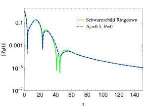
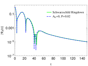
Figure 3: This figure evaluated at $r=5r_{+}$ for $l=0$. Either panel indicates the time evolution of the wave function $\Psi_{0}\left(t\right)$ of scalar perturbations for fixed value of one LQG correction parameter while setting the other one equals to zero.

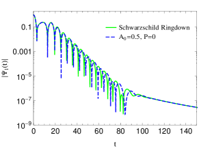
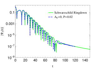
Figure 4: This figure evaluated at $r=5r_{+}$ for $l=1$. Either panel indicates the time evolution of the wave function $\Psi_{1}\left(t\right)$ of scalar perturbations at early, intermediate, and late times. The ringdown waveform is plotted for fixed value of one LQG correction parameter while setting the other one equals to zero.

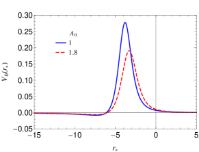
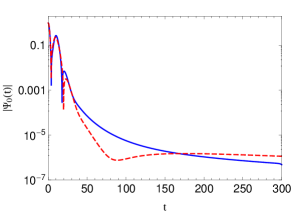
Figure 5: The effective potential versus tortoise coordinate for $l=0$ and $P=0.9$ with a negative gap (left panel), and the time evolution of the corresponding mode $\Psi_{0}\left(t\right)$ (right panel).

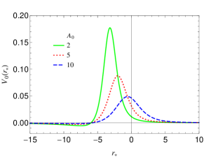
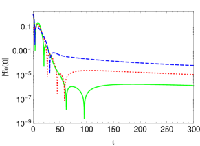
Figure 6: The effective potential versus tortoise coordinate for $l=0$ and $P=0.9$ with a negative gap (left panel), and the time evolution of the corresponding mode $\Psi_{0}\left(t\right)$ (right panel).

Now, we look for the lowest overtone and obtain the QNMs for various values of the free parameters $P$ and $A_{0}$ to investigate the effects of the LQG corrections on the QN frequencies and find deviations from those of the Schwarzschild BHs. Tables 3-5 show the effect of the minimum area gap of LQG $A_{0}$ on the QN frequencies. Although the free parameter $A_{0}$ is a small quantity, we have chosen large values to see its effects on the QN frequencies. Besides, Tables 6-8 show the effect of the polymeric function $P$ on the QN frequencies. The QNMs were calculated for $M=1/2$ and the rows corresponding to $A_{0}=0$ and $P=0$ indicate the Schwarzschild QN frequencies.

By considering Tables 3-5, one can see that both the real and imaginary parts of the QN frequencies decrease with an increase in $A_{0}$. Therefore, the perturbations in the background spacetime of LQBHs with non-zero $A_{0}$ live longer with fewer oscillations in comparison with the Schwarzschild solutions. However, Tables 6-8 show an opposite behavior for the polymeric function $P$. In this case, the real part of frequencies and damping rate increase as $P$ increases, and thus, the perturbations in the background of LQBHs with non-zero $P$ enjoy faster decay with more oscillations compared to the Schwarzschild BHs. In Ref. BarrauUniverse , it has been stated that the polymerization does not affect the damping rate of QNMs, whereas one can obviously see the effects of $P$ on the imaginary part of the QN frequencies in Tables 6-8. However, note that the polymeric function affects the real part much more than the imaginary part, and this fact may lead to a misleading conclusion so that the polymerization does not affect the damping rate. We also see that the $6$th order WKB formula is in good agreement with the AIM results for $n<l$ and low values of the LQG correction parameters (we shall discuss the higher-order WKB formula and related Padé approximants in the next section).

The effects of $A_{0}$ and $P$ on the QNMs that are described above, do not exactly coincide with the picture given in Chen2011 as well. This is because the dominant fundamental mode $n=0=l$ was calculated with the help of usual $3$rd order WKB formula while this formula does not give reliable frequencies for $n\geq l$. More importantly, for some higher values of $A_{0}$ and $P$ (say $A_{0}\geq 1$ and $P\geq 0.9$ that was considered in Chen2011 ), a negative gap appears in the effective potential (9) such that the WKB expansion could not be performed. This negative gap appears for the lowest multipole number ($l=0$) that may lead to instability (see Figs. 5-6 and related discussion below).

From Tables 3-8, we find two important differences between the LQG correction quantities $A_{0}$ and $P$. First, one can see that the effects of the polymeric function $P$ on the QNMs are much higher than the minimum area gap $A_{0}$. Therefore, the polymeric function $P$ plays a more important role in the evolution of fields on the background geometry of LQBHs compared with $A_{0}$. Second, the LQG correction parameters affect the value of the QNMs differently. In other words, both the real and imaginary parts decrease as $A_{0}$ increases, whereas they increase as $P$ increases.

Furthermore, the time-domain profile of modes is illustrated in Figs. 3 and 4 for fixed value of one LQG correction parameter while setting the other one equal to zero. According to the time evolution of modes, we can observe three different stages of QN oscillations of the wave function $\Psi_{l}\left(t,r\right)$ at early, intermediate, and late times for $l=0,1$. First, note that by considering the contribution of all modes, both the real and imaginary parts still decrease as $A_{0}$ increases (the left panels of Figs. 3 and 4) whereas they increase as $P$ increases (the right panels of Figs. 3 and 4) that confirm results deduced from Tables 3-8. Second, we see that although the time evolution of scalar field in the background of LQBHs differ from the Schwarzschild ones at intermediate times, this is not the case for the late times and both BH solutions seem to share the same power-law tail as $\Psi_{l}\left(t\right)\sim t^{-(2l+3)}$ SchwTail .

In addition, by employing the Prony method to fit the data in Figs. 3 and 4, we calculated the longest-lived modes $\omega_{00}$ as

$$\left\{\begin{array}[]{cc}0.221015-0.209788i,&\text{for Schwarzschild BH, }\\ 0.200820-0.205698i,&\text{for }A_{0}=0.5\text{, }P=0\text{, }\\ 0.229522-0.218754i,&\text{for }A_{0}=0\text{, }P=0.02\text{,}\end{array}\right.$$ (36)

for $l=0$ which coincide with results in Tables 3 and 6. The results of $\omega_{01}$ (for $l=1$) are

$$\left\{\begin{array}[]{cc}0.585883-0.195323i,&\text{for Schwarzschild BH, }\\ 0.557644-0.192999i,&\text{for }A_{0}=0.5\text{, }P=0\text{, }\\ 0.616512-0.203837i,&\text{for }A_{0}=0\text{, }P=0.02\text{,}\end{array}\right.$$ (37)

and they are in a good agreement with the Tables 3 and 6 as well.

As for the dynamic stability of our BH case study, Figs. 3 and 4 show that the perturbations decay in time for small values of $A_{0}$ and $P$, and also, the effective potential (9) is positive definite (see Fig. 2). These conditions guarantee the dynamical stability of the LQBHs undergoing scalar perturbations.

We recall that for some higher values of $A_{0}$ and $P$ (say $A_{0}\geq 1$ and $P\geq 0.9$), a negative gap appears in the effective potential for the lowest multipole number (see the left panel of Figs. 5 and 6). This negative gap may lead to a bound state with negative energy, hence a growing mode will appear in the spectrum and dominate at late time which means dynamic instability (see InstabilityKZ ; InstabilityWang  as examples of dynamic instability of low-$l$ modes). Therefore, we should check the stability for this case numerically while the contribution of all the modes is taken into account.

The right panel of Figs. 5 and 6 show that the perturbations decay in time that indicate the dynamical stability of the BHs. In the right panel of Fig. 5 and for $A_{0}=1.8$, the asymptotic tail of modes first starts to grow but finally decays at late time. However, note that the LQG correction parameters $A_{0}$ and $P$ are very small quantities by definition, and we examined the large $A_{0}$ and $P$ case to complete the discussion. The important point is that the BHs are dynamically stable for small $A_{0}$ and $P$ as demonstrated in Figs. 2-4.

III.1 Higher-order WKB formula and Padé approximants

As the final remark, we should note that, usually, employing the numerical methods to obtain the QNMs is hard, and normally one needs to modify the approach based on the different effective potentials. On the other hand, the WKB approximation provides quite a simple, powerful, and accurate tool for investigating the dynamical properties of BHs in some cases. However, generally, this method does not always give a reliable result and neither guarantees a good estimation for the error KonoplyaPade . Besides, we cannot always increase the WKB order to obtain a more accurate frequency due to the fact that the WKB formula (12) asymptotically approaches the QNMs. So, there is an order of the WKB formula that provides the best approximation and the error increases as the order of the formula increases. Thus, it will be helpful to find the most accurate WKB order and related Padé approximation for calculating the QN frequencies of LQBHs.

In order to estimate the error of the WKB approximation (12), we use the following quantity KonoplyaPade

$$\Delta_{k}=\frac{\left|\omega_{k+1}-\omega_{k-1}\right|}{2},$$ (38)

because each WKB correction term affects either the real or imaginary part of the squared frequencies. This relation obtains the error estimation of $\omega_{k}$ that is calculated with the WKB formula of the $k$th order, and the minimum value of $\Delta_{k}$ usually gives the WKB order in which the error is minimal. It was shown that $\Delta_{k}$ provides a good estimation of the error order for the Schwarzschild BH, usually satisfying KonoplyaPade

$$\Delta_{k}\gtrsim\delta_{k}=\left|\omega-\omega_{k}\right|,$$ (39)

where $\omega$ is the accurate value of the quasinormal frequency. The quantity $\Delta_{k}$ has been also used to estimate the error of WKB formula in conformal Weyl gravity MomenniaWeyl , and the results mostly have satisfied the condition (39) as well.

Here, we check the validity of the condition (39) for our BH case study to see if the minimal $\Delta_{k}$ gives the most accurate WKB order, and results are given in Tables 11-14. The minimal $\Delta_{k}$ and $\delta_{k}$ are denoted in bold style. By considering these tables, we find that the condition (39) is valid for LQBHs in all cases as for the Schwarzschild BHs and conformal Weyl solutions. More interestingly, we see that to obtain the QN frequencies by employing the higher-order WKB formula (12), the minimal $\Delta_{k}$ usually identifies the most accurate WKB order.

In addition, the QN modes are calculated through the various orders of Padé approximation and results are presented in Tables 14-16. The bold values denote the minimal SD and $\delta_{k}$. From these tables, it is clear that the minimal SD coincides with the minimal $\delta_{k}$ except for $n=0=l$. Thus, the minimum SD gives the most accurate result that could be obtained through the Padé approximants. On the other hand, by comparing Tables 11-14 with Tables 14-16 in order, we see how Padé approximants increase the accuracy of the WKB formula. Therefore, even for the case $n=0=l$, employing the Padé approximation with minimal SD is more accurate than the ordinary WKB approximation, as we expected.

$k$		$\omega_{k}\left(l=0\right)$	$\Delta_{k}$	$\delta_{k}$			$\omega_{k}\left(l=1\right)$	$\Delta_{k}$	$\delta_{k}$
$1$		$0.3813-0.2084i$	$-$	$0.1806$			$0.6398-0.1962i$	$-$	$0.0823$
$2$		$0.2474-0.3212i$	$0.1219$	$0.1245$			$0.5574-0.2252i$	$0.0476$	$0.0322$
$3$		$0.1409-0.2487i$	$0.0696$	$0.0737$			$0.5447-0.1917i$	$0.0192$	$0.0130$
$4$		$0.1713-0.2046i$	$\mathbf{0.0341}$	$\mathbf{0.0296}$			$0.5590-0.1868i$	$0.0087$	$0.0064$
$5$		$0.1416-0.1805i$	$0.0530$	$0.0643$			$0.5617-0.1948i$	$\mathbf{0.0061}$	$\mathbf{0.0045}$
$6$		$0.2254-0.1134i$	$0.0712$	$0.0955$			$0.5537-0.1977i$	$0.0085$	$0.0061$
$7$		$0.2821-0.2041i$	$0.0810$	$0.0813$			$0.5488-0.1837i$	$0.0168$	$0.0128$
$8$		$0.2097-0.2746i$	$0.0994$	$0.0695$			$0.5780-0.1744i$	$0.0349$	$0.0276$
$9$		$0.3488-0.3913i$	$0.6479$	$0.2374$			$0.5983-0.2330i$	$0.0751$	$0.0571$
$10$		$0.0872-1.5646i$	$>1$	$>1$			$0.4815-0.2896i$	$0.1527$	$0.1230$
$11$		$2.0551+2.5815i$	$>1$	$>1$			$0.3850-0.0146i$	$0.1504$	$0.2483$
$12$		$2.4757+2.1429i$	$>1$	$>1$			$0.5914-0.0095i$	$0.5055$	$0.1866$
$13$		$11.41+11.35i$	$-$	$>1$			$0.9907+0.7949i$	$-$	$>1$

Table 9: The QN modes calculated by the WKB formula of different orders for $P=0$, $A_{0}=0.5$, $n=0$, $l=0$ (left), and $l=1$ (right). The minimum value of $\Delta_{k}$ and $\delta_{k}$ are given in bold. The accurate modes $\omega_{00}=0.2008-0.2057i$ and $\omega_{01}=0.5576-0.1930i$ are taken from Table 3.

$k$		$\omega_{k}\left(l=1\right)$	$\Delta_{k}$	$\delta_{k}$			$\omega_{k}\left(l=2\right)$	$\Delta_{k}$	$\delta_{k}$
$1$		$0.7780-0.4841i$	$-$	$0.3292$			$1.0872-0.5181i$	$-$	$0.2269$
$2$		$0.5385-0.6994i$	$0.1858$	$0.1195$			$0.8906-0.6324i$	$0.1194$	$0.0541$
$3$		$0.4328-0.6216i$	$0.0701$	$0.0426$			$0.8581-0.5858i$	$0.0290$	$0.0120$
$4$		$0.4628-0.5814i$	$0.0292$	$0.0213$			$0.8686-0.5786i$	$0.0067$	$0.0040$
$5$		$0.4876-0.6014i$	$\mathbf{0.0230}$	$\mathbf{0.0173}$			$0.8712-0.5824i$	$0.0025$	$0.0016$
$6$		$0.4676-0.6271i$	$0.0319$	$0.0259$			$0.8694-0.5836i$	$\mathbf{0.0014}$	$\mathbf{0.0011}$
$7$		$0.4241-0.5953i$	$0.0533$	$0.0465$			$0.8684-0.5820i$	$0.0017$	$0.0013$
$8$		$0.4840-0.5217i$	$0.0742$	$0.0807$			$0.8708-0.5804i$	$0.0032$	$0.0025$
$9$		$0.5722-0.6045i$	$0.0605$	$0.1020$			$0.8739-0.5850i$	$0.0064$	$0.0050$
$10$		$0.5735-0.6031i$	$0.3579$	$0.1032$			$0.8645-0.5914i$	$0.0133$	$0.0102$
$11$		$1.0865-1.1024i$	$>1$	$0.7943$			$0.8510-0.5715i$	$0.0286$	$0.0216$
$12$		$0.3583-3.3435i$	$>1$	$>1$			$0.8953-0.5432i$	$0.0637$	$0.0469$
$13$		$4.6774+5.7383i$	$-$	$>1$			$0.9577-0.6409i$	$-$	$0.1057$

Table 10: The QN modes calculated by the WKB formula of different orders for $P=0$, $A_{0}=0.5$, $n=1$, $l=1$ (left), and $l=2$ (right). The minimum value of $\Delta_{k}$ and $\delta_{k}$ are given in bold. The accurate modes $\omega_{11}=0.4703-0.6013i$ and $\omega_{12}=0.8696-0.5825i$ are taken from Table 4.

$k$		$\omega_{k}\left(l=0\right)$	$\Delta_{k}$	$\delta_{k}$			$\omega_{k}\left(l=1\right)$	$\Delta_{k}$	$\delta_{k}$
$1$		$0.3948-0.2043i$	$-$	$0.1656$			$0.6920-0.2009i$	$-$	$>10^{-3}$
$2$		$0.2754-0.2930i$	$0.0903$	$0.0876$			$0.6197-0.2244i$	$>10^{-3}$	$>10^{-3}$
$3$		$0.2177-0.2396i$	$0.0399$	$0.0246$			$0.6128-0.2045i$	$>10^{-3}$	$>10^{-3}$
$4$		$0.2280-0.2288i$	$0.0099$	$0.0107$			$0.6165-0.2033i$	$>10^{-3}$	$0.00051$
$5$		$0.2191-0.2199i$	$0.0096$	$0.0108$			$0.6168-0.2039i$	$0.0003713$	$0.00029$
$6$		$0.2298-0.2097i$	$0.0082$	$0.0085$			$0.6165-0.2040i$	$0.0001834$	$0.00024$
$7$		$0.2349-0.2153i$	$\mathbf{0.0061}$	$\mathbf{0.0059}$			$0.6164-0.2038i$	$0.0001122$	$0.00011$
$8$		$0.2420-0.2090i$	$0.0194$	$0.0153$			$0.6165-0.2038i$	$\mathbf{0.0000462}$	$\mathbf{<5\times 10}^{-5}$
$9$		$0.2669-0.2373i$	$0.0298$	$0.0417$			$0.6165-0.2038i$	$0.0000610$	$\mathbf{<5\times 10}^{-5}$
$10$		$0.2361-0.2682i$	$0.0436$	$0.0504$			$0.6166-0.2038i$	$0.0001349$	$0.00011$
$11$		$0.2938-0.3202i$	$0.1872$	$0.1204$			$0.6167-0.2040i$	$0.0002370$	$0.00025$
$12$		$0.1488-0.6323i$	$0.4874$	$0.4220$			$0.6163-0.2041i$	$0.0003873$	$0.00038$
$13$		$0.2165+0.6516i$	$-$	$0.8699$			$0.6161-0.2035i$	$-$	$0.00052$

Table 11: The QN modes calculated by the WKB formula of different orders for $A_{0}=0$, $P=0.02$, $n=0$, $l=0$ (left), and $l=1$ (right). The minimum value of $\Delta_{k}$ and $\delta_{k}$ are given in bold. The accurate modes $\omega_{00}=0.2298-0.2182i$ and $\omega_{01}=0.6165-0.2038i$ are taken from Table 6.

$k$		$\omega_{k}\left(l=1\right)$	$\Delta_{k}$	$\delta_{k}$			$\omega_{k}\left(l=2\right)$	$\Delta_{k}$	$\delta_{k}$
$1$		$0.8310-0.5019i$	$-$	$>10^{-2}$			$1.1798-0.5442i$	$-$	$>10^{-2}$
$2$		$0.6067-0.6875i$	$>10^{-2}$	$>10^{-2}$			$0.9949-0.6453i$	$>10^{-2}$	$>10^{-2}$
$3$		$0.5536-0.6410i$	$>10^{-2}$	$0.00501$			$0.9771-0.6176i$	$>10^{-2}$	$0.00142$
$4$		$0.5564-0.6378i$	$0.002423$	$0.00184$			$0.9783-0.6169i$	$0.0007025$	$0.00041$
$5$		$0.5581-0.6392i$	$0.001103$	$0.00054$			$0.9785-0.6172i$	$0.0002033$	$\mathbf{<5\times 10}^{-5}$
$6$		$0.5581-0.6392i$	$\mathbf{0.000168}$	$0.00050$			$0.9785-0.6172i$	$0.0000281$	$\mathbf{<5\times 10}^{-5}$
$7$		$0.5579-0.6390i$	$0.000189$	$0.00031$			$0.9784-0.6172i$	$0.0000297$	$0.00007$
$8$		$0.5580-0.6388i$	$0.000205$	$\mathbf{0.00014}$			$0.9785-0.6172i$	$0.0000196$	$\mathbf{<5\times 10}^{-5}$
$9$		$0.5577-0.6386i$	$0.000399$	$0.00032$			$0.9785-0.6172i$	$0.0000082$	$\mathbf{<5\times 10}^{-5}$
$10$		$0.5582-0.6381i$	$0.000728$	$0.00066$			$0.9785-0.6172i$	$0.0000048$	$\mathbf{<5\times 10}^{-5}$
$11$		$0.5591-0.6389i$	$0.001194$	$0.00114$			$0.9785-0.6172i$	$0.0000029$	$\mathbf{<5\times 10}^{-5}$
$12$		$0.5578-0.6404i$	$0.001858$	$0.00173$			$0.9785-0.6172i$	$\mathbf{0.0000021}$	$\mathbf{<5\times 10}^{-5}$
$13$		$0.5554-0.6384i$	$-$	$0.00258$			$0.9785-0.6172i$	$-$	$\mathbf{<5\times 10}^{-5}$

Table 12: The QN modes calculated by the WKB formula of different orders for $A_{0}=0$, $P=0.02$, $n=1$, $l=1$ (left), and $l=2$ (right). The minimum value of $\Delta_{k}$ and $\delta_{k}$ are given in bold. The accurate modes $\omega_{11}=0.5580-0.6387i$ and $\omega_{12}=0.9785-0.6172i$ are taken from Table 7.

$k$		$\omega_{k}\left(l=0\right)$	SD	$\delta_{k}$			$\omega_{k}\left(l=1\right)$	SD	$\delta_{k}$
$1$		$0.2937-0.1605i$	$>10^{-2}$	$>10^{-2}$			$0.5848-0.1794i$	$>10^{-2}$	$>10^{-2}$
$2$		$0.2089-0.1827i$	$>10^{-2}$	$>10^{-2}$			$0.5563-0.1913i$	$0.005019$	$0.00214$
$3$		$0.1982-0.1962i$	$0.003302$	$0.00985$			$0.5571-0.1918i$	$0.000329$	$0.00126$
$4$		$0.1989-0.1965i$	$\mathbf{0.000304}$	$0.00937$			$0.5582-0.1928i$	$0.000582$	$0.00067$
$5$		$0.2012-0.1965i$	$0.003240$	$0.00917$			$0.5571-0.1932i$	$0.000337$	$0.00056$
$6$		$0.2040-0.2001i$	$0.000858$	$0.00647$			$0.5576-0.1928i$	$0.000188$	$0.00022$
$7$		$0.2037-0.1996i$	$0.000387$	$0.00677$			$0.5576-0.1928i$	$0.000142$	$0.00015$
$8$		$0.2046-0.2002i$	$0.001148$	$0.00669$			$0.5577-0.1929i$	$0.000068$	$0.00014$
$9$		$0.2036-0.1995i$	$0.000410$	$0.00682$			$0.5577-0.1930i$	$0.000178$	$0.00014$
$10$		$0.2046-0.2006i$	$0.001567$	$0.00630$			$0.5577-0.1930i$	$0.000023$	$0.00008$
$11$		$0.2076-0.1967i$	$0.008442$	$>10^{-2}$			$0.5577-0.1930i$	$0.000048$	$0.00007$
$12$		$0.1996-0.2054i$	$0.004183$	$\mathbf{0.00125}$			$0.5577-0.1930i$	$0.000074$	$0.00007$
$13$		$0.2019-0.2083i$	$0.009697$	$0.00281$			$0.5576-0.1930i$	$\mathbf{0.000007}$	$\mathbf{<5\times 10}^{-5}$

Table 13: The QN modes calculated by averaging of Padé approximations of different orders for $P=0$, $A_{0}=0.5$, $n=0$, $l=0$ (left), and $l=1$ (right). The minimal SD and $\delta_{k}$ are given in bold. The accurate modes $\omega_{00}=0.2008-0.2057i$ and $\omega_{01}=0.5576-0.1930i$ are taken from Table 3.

$k$		$\omega_{k}\left(l=1\right)$	SD	$\delta_{k}$			$\omega_{k}\left(l=2\right)$	SD	$\delta_{k}$
$1$		$0.5608-0.3490i$	$>10^{-2}$	$>10^{-2}$			$0.8860-0.4222i$	$>10^{-2}$	$>10^{-2}$
$2$		$0.5161-0.5923i$	$>10^{-2}$	$>10^{-2}$			$0.8829-0.5814i$	$>10^{-2}$	$>10^{-2}$
$3$		$0.4539-0.6082i$	$>10^{-2}$	$>10^{-2}$			$0.8642-0.5834i$	$0.006589$	$0.00543$
$4$		$0.4694-0.5918i$	$0.007131$	$0.00952$			$0.8694-0.5805i$	$0.001170$	$0.00198$
$5$		$0.4731-0.6019i$	$0.006718$	$0.00285$			$0.8702-0.5823i$	$0.000844$	$0.00062$
$6$		$0.4661-0.6026i$	$0.001203$	$0.00443$			$0.8693-0.5828i$	$0.000094$	$0.00042$
$7$		$0.4715-0.5943i$	$>10^{-2}$	$0.00708$			$0.8696-0.5822i$	$0.000386$	$0.00031$
$8$		$0.4702-0.6005i$	$0.000487$	$0.00083$			$0.8697-0.5826i$	$0.000032$	$0.00013$
$9$		$0.4726-0.6115i$	$>10^{-2}$	$>10^{-2}$			$0.8696-0.5826i$	$0.000031$	$0.00007$
$10$		$0.4965-0.6019i$	$>10^{-2}$	$>10^{-2}$			$0.8696-0.5825i$	$0.000011$	$\mathbf{<5\times 10}^{-5}$
$11$		$0.4703-0.6017i$	$0.000198$	$0.00037$			$0.8696-0.5826i$	$0.000027$	$0.00007$
$12$		$0.4703-0.6014i$	$\mathbf{0.000174}$	$\mathbf{0.00011}$			$0.8696-0.5825i$	$0.000010$	$\mathbf{<5\times 10}^{-5}$
$13$		$0.4698-0.6015i$	$0.000338$	$0.00051$			$0.8696-0.5825i$	$\mathbf{0.000008}$	$\mathbf{<5\times 10}^{-5}$

Table 14: The QN modes calculated by averaging of Padé approximations of different orders for $P=0$, $A_{0}=0.5$, $n=1$, $l=1$ (left), and $l=2$ (right). The minimal SD and $\delta_{k}$ are given in bold. The accurate modes $\omega_{11}=0.4703-0.6013i$ and $\omega_{12}=0.8696-0.5825i$ are taken from Table 4.

$k$		$\omega_{k}\left(l=0\right)$	SD	$\delta_{k}$			$\omega_{k}\left(l=1\right)$	SD	$\delta_{k}$
$1$		$0.3114-0.1612i$	$>10^{-2}$	$>10^{-2}$			$0.6382-0.1853i$	$>10^{-4}$	$>10^{-3}$
$2$		$0.2375-0.1917i$	$>10^{-2}$	$>10^{-2}$			$0.6166-0.2010i$	$>10^{-4}$	$>10^{-3}$
$3$		$0.2309-0.2085i$	$0.004396$	$0.00974$			$0.6161-0.2032i$	$>10^{-4}$	$0.00075$
$4$		$0.2284-0.2220i$	$0.007874$	$0.00403$			$0.6166-0.2038i$	$>10^{-4}$	$0.00007$
$5$		$0.2314-0.2156i$	$0.001599$	$0.00303$			$0.6166-0.2039i$	$0.00008569$	$0.00013$
$6$		$0.2316-0.2175i$	$0.001262$	$0.00192$			$0.6165-0.2038i$	$0.00000082$	$\mathbf{<5\times 10}^{-5}$
$7$		$0.2328-0.2171i$	$0.000709$	$0.00324$			$0.6165-0.2038i$	$\mathbf{0.00000001}$	$\mathbf{<5\times 10}^{-5}$
$8$		$0.2305-0.2180i$	$0.000175$	$0.00071$			$0.6165-0.2038i$	$0.00000094$	$\mathbf{<5\times 10}^{-5}$
$9$		$0.2295-0.2183i$	$0.001963$	$\mathbf{0.00032}$			$0.6165-0.2038i$	$0.00002807$	$\mathbf{<5\times 10}^{-5}$
$10$		$0.2300-0.2178i$	$0.000837$	$0.00047$			$0.6165-0.2038i$	$0.00000233$	$\mathbf{<5\times 10}^{-5}$
$11$		$0.2303-0.2181i$	$\mathbf{0.000675}$	$0.00053$			$0.6165-0.2038i$	$0.00000018$	$\mathbf{<5\times 10}^{-5}$
$12$		$0.2310-0.2181i$	$0.001046$	$0.00121$			$0.6165-0.2038i$	$0.00000004$	$\mathbf{<5\times 10}^{-5}$
$13$		$0.2302-0.2183i$	$0.000868$	$0.00043$			$0.6165-0.2038i$	$0.00000008$	$\mathbf{<5\times 10}^{-5}$

Table 15: The QN modes calculated by averaging of Padé approximations of different orders for $A_{0}=0$, $P=0.02$, $n=0$, $l=0$ (left), and $l=1$ (right). The minimal SD and $\delta_{k}$ are given in bold. The accurate modes $\omega_{00}=0.2298-0.2182i$ and $\omega_{01}=0.6165-0.2038i$ are taken from Table 6.

$k$		$\omega_{k}\left(l=1\right)$	SD	$\delta_{k}$			$\omega_{k}\left(l=2\right)$	SD	$\delta_{k}$
$1$		$0.6088-0.3678i$	$>10^{-2}$	$>10^{-2}$			$0.9729-0.4487i$	$>10^{-4}$	$>10^{-3}$
$2$		$0.5875-0.6015i$	$>10^{-2}$	$>10^{-2}$			$0.9881-0.6033i$	$>10^{-4}$	$>10^{-3}$
$3$		$0.5602-0.6363i$	$0.008200$	$0.00330$			$0.9794-0.6166i$	$>10^{-4}$	$>10^{-3}$
$4$		$0.5562-0.6372i$	$0.001406$	$0.00238$			$0.9782-0.6167i$	$>10^{-4}$	$0.00052$
$5$		$0.5576-0.6394i$	$0.000505$	$0.00081$			$0.9784-0.6172i$	$0.00005898$	$0.00008$
$6$		$0.5581-0.6392i$	$0.000040$	$0.00047$			$0.9785-0.6172i$	$0.00000197$	$\mathbf{<5\times 10}^{-5}$
$7$		$0.5579-0.6391i$	$0.000116$	$0.00042$			$0.9784-0.6172i$	$0.00001819$	$0.00006$
$8$		$0.5580-0.6390i$	$0.000030$	$0.00027$			$0.9785-0.6172i$	$0.00000141$	$\mathbf{<5\times 10}^{-5}$
$9$		$0.5577-0.6387i$	$0.000187$	$0.00026$			$0.9785-0.6172i$	$0.00000410$	$\mathbf{<5\times 10}^{-5}$
$10$		$0.5582-0.6389i$	$0.000331$	$0.00029$			$0.9785-0.6172i$	$0.00000112$	$\mathbf{<5\times 10}^{-5}$
$11$		$0.5581-0.6388i$	$0.000188$	$0.00010$			$0.9785-0.6172i$	$0.00000010$	$\mathbf{<5\times 10}^{-5}$
$12$		$0.5580-0.6387i$	$0.000019$	$\mathbf{<5\times 10}^{-5}$			$0.9785-0.6172i$	$0.00000043$	$\mathbf{<5\times 10}^{-5}$
$13$		$0.5580-0.6387i$	$\mathbf{0.000008}$	$\mathbf{<5\times 10}^{-5}$			$0.9785-0.6172i$	$\mathbf{0.00000007}$	$\mathbf{<5\times 10}^{-5}$

Table 16: The QN modes calculated by averaging of Padé approximations of different orders for $A_{0}=0$, $P=0.02$, $n=1$, $l=1$ (left), and $l=2$ (right). The minimal SD and $\delta_{k}$ are given in bold. The accurate modes $\omega_{11}=0.5580-0.6387i$ and $\omega_{12}=0.9785-0.6172i$ are taken from Table 7.

IV Conclusions

We have considered a minimally coupled scalar perturbation in the background spacetime of the LQG-corrected BHs characterized by two LQG correction parameters, namely, the polymeric function $P$ and the minimum area gap $A_{0}$. We have calculated the corresponding QN modes with the help of three independent methods of calculations; the higher-order WKB formula and related Padé approximants, the improved AIM, and time-domain integration. The effects of LQG correction parameters on the QNMs spectrum have been studied and deviations from those of the Schwarzschild BHs have been investigated.

We have found that the QNMs were more sensitive to changes in the polymeric function $P$ compared with the minimum area gap $A_{0}$. Thus, $P$ plays a more important role in the evolution of fields on the background geometry of LQBHs compared with $A_{0}$. In addition, we have shown that the LQG correction parameters had opposite effects on the QN frequencies. Increasing in $P$ ($A_{0}$) led to increasing (decreasing) in the real part of frequencies and damping rate. While one of the free parameters increases the lifetime of perturbations, the other one attempts to dissipate perturbations faster. These cases have been also confirmed through the time-domain profile of perturbations by considering the contribution of all modes. We have also calculated the dominant QN frequencies by employing the Prony method which was in good agreement with the results of AIM.

In addition, we have seen that the effective potential of perturbations was positive definite and the modes decayed in time that guaranteed the dynamical stability of the LQBHs undergoing scalar perturbations. Although a negative gap appeared in the effective potential for the lowest multipole number and higher values of the LQG correction parameters, the perturbations decayed in time which indicated dynamical stability of the BHs.

We have used the higher-order WKB formula and related Padé approximants as a semi-analytic method to obtain the QNMs and find the most accurate order of the WKB and Padé approximations for calculating the QN frequencies. It was shown that the minimum value of error estimation quantity, denoted by $\Delta_{k}$ throughout the text, provides a good estimation for the error and usually gives the most accurate WKB order. Besides, we have seen that by employing the averaging of Padé approximations, one can increase the accuracy of modes considerably compared to the ordinary WKB formula and obtain accurate modes for $n<l$.

References

- (1) K. D. Kokkotas and B. G. Schmidt, Living Rev. Rel. 2, 2 (1999).
- (2) E. Berti, V. Cardoso and A. O. Starinets, Class. Quant. Grav. 26, 163001 (2009).
- (3) R. A. Konoplya and A. Zhidenko, Rev. Mod. Phys. 83, 793 (2011).
- (4) B. P. Abbott et al. (LIGO Scientific and Virgo Collaborations), Phys. Rev. Lett. 116, 061102 (2016).
- (5) B. P. Abbott et al. (LIGO Scientific and Virgo Collaborations), Phys. Rev. Lett. 119, 161101 (2017).
- (6) M. Isi, M. Giesler, W. M. Farr, M. A. Scheel and S. A. Teukolsky, Phys. Rev. Lett. 123, 111102 (2019).
- (7) E. Berti, V. Cardoso and C. M. Will, Phys. Rev. D 73, 064030 (2006).
- (8) L. Barack et al., Class. Quant. Grav. 36, 143001 (2019).
- (9) S. Hod, Phys. Rev. Lett. 81, 4293 (1998).
- (10) O. Dreyer, Phys. Rev. Lett. 90, 081301 (2003).
- (11) G. T. Horowitz and V. E. Hubeny, Phys. Rev. D 62, 024027 (2000).
- (12) V. Cardoso and J. P. S. Lemos, Phys. Rev. D 64, 084017 (2001).
- (13) E. Berti and K. D. Kokkotas, Phys. Rev. D 67, 064020 (2003).
- (14) S. H. Hendi and M. Momennia, JHEP 10, 207 (2019).
- (15) M. Momennia, S. H. Hendi and F. Soltani Bidgoli, Phys. Lett. B 813, 136028 (2021).
- (16) V. Cardoso, A. S. Miranda, E. Berti, H. Witek and V. T. Zanchin, Phys. Rev. D 79, 064016 (2009).
- (17) R. A. Konoplya, Z. Stuchlik and A. Zhidenko, Phys. Rev. D 98, 104033 (2018).
- (18) M. Momennia and S. H. Hendi, Phys. Rev. D 99, 124025 (2019).
- (19) G. Gubitosi, F. Piazza and F. Vernizzi, JCAP 02, 032 (2013).
- (20) W. Hu, R. Barkana and A. Gruzinov, Phys. Rev. Lett. 85, 1158 (2000).
- (21) C. Cheung et al., JHEP 03, 014 (2008).
- (22) R. Metsaev and A. Tseytlin, Nucl. Phys. B 293, 385 (1987).
- (23) A. Arvanitaki et al., Phys. Rev. D 81, 123530 (2010).
- (24) C. A. R. Herdeiro and E. Radu, Phys. Rev. Lett. 112, 221101 (2014).
- (25) H. O. Silva et al., Phys. Rev. Lett. 120, 131104 (2018).
- (26) R. Brito, V. Cardoso and P. Pani, Lect. Notes Phys. 906, 1 (2015).
- (27) O. J. Tattersall and P. G. Ferreira, Phys. Rev. D 97, 104047 (2018).
- (28) C. Dalang, P. Fleury and L. Lombriser, Phys. Rev. D 103, 064075 (2021).
- (29) A. Maselli et al., Nat. Astron. 6, 464 (2022).
- (30) Y. Guo and Y. G. Miao, Phys. Rev. D 102, 084057 (2020).
- (31) H. Ma and J. Li, Chin. Phys. C 44, 095102 (2020).
- (32) P. Burikham, S. Ponglertsakul and T. Wuthicharn, Eur. Phys. J. C 80, 954 (2020).
- (33) M. Bouhmadi-Lopez, S. Brahma, C. Y. Chen, P. Chen and D. Yeom, JCAP 07, 066 (2020).
- (34) M. Wang, Z. Chen, Q. Pan and J. Jing, Eur. Phys. J. C 81, 469 (2021).
- (35) J. Matyjasek, Phys. Rev. D 102, 124046 (2020).
- (36) S. H. Hendi, S. Hajkhalili, M. Jamil and M. Momennia, Eur. Phys. J. C 81, 1112 (2021).
- (37) M. Sharif and Z. Akhtar, Phys. Dark Universe 29, 100589 (2020).
- (38) L. Modesto, Int. J. Theor. Phys. 49, 1649 (2010).
- (39) A. Perez, Rep. Prog. Phys. 80, 126901 (2017).
- (40) A. Barrau, K. Martineau and F. Moulin, Universe 4, 102 (2018).
- (41) S. J. Yang, Y. P. Zhang, S. W. Wei and Y. X. Liu, JHEP 04, 066 (2022).
- (42) E. Alesci and L. Modesto, Gen. Rel. Grav. 46, 1656 (2014).
- (43) S. Sahu, K. Lochan and D. Narasimha, Phys. Rev. D 91, 063001 (2015).
- (44) C. Liu, T. Zhu, Q. Wu, K. Jusufi, M. Jamil, M. Azreg-Ainou and A. Wang, Phys. Rev. D 101, 084001 (2020) [Erratum: Phys. Rev. D 103, 089902 (2021)].
- (45) J. H. Chen and Y. J. Wang, Chin. Phys. B 20, 030401 (2011).
- (46) F. Moulin, A. Barrau and K. Martineau, Universe 5, 202 (2019).
- (47) B. F. Schutz and C. M. Will, Astrophys. J. Lett. 291, L33 (1985).
- (48) S. Iyer and C. M. Will, Phys. Rev. D 35, 3621 (1987).
- (49) R. A. Konoplya, Phys. Rev. D 68, 024018 (2003).
- (50) J. Matyjasek and M. Opala, Phys. Rev. D 96, 024011 (2017).
- (51) R. A. Konoplya, A. Zhidenko and A. F. Zinhailo, Class. Quant. Grav. 36, 155002 (2019).
- (52) H. Ciftci, R. L. Hall and N. Saad, J. Phys. A 36, 11807 (2003).
- (53) H. Ciftci, R. L. Hall and N. Saad, Phys. Lett. A 340, 388 (2005).
- (54) H. T. Cho, A. S. Cornell, J. Doukas and W. Naylor, Class. Quant. Grav. 27, 155004 (2010).
- (55) H. T. Cho, A. S. Cornell, J. Doukas, T. R. Huang and W. Naylor, Adv. Math. Phys. 2012, 281705 (2012).
- (56) E. W. Leaver, Proc. R. Soc. Lond. A 402, 285 (1985).
- (57) E. W. Leaver, Phys. Rev. D 41, 2986 (1990).
- (58) C. Gundlach, R. H. Price and J. Pullin, Phys. Rev. D 49, 883 (1994).
- (59) S. L. Marple, Digital spectral analysis with applications, (Prentice-Hall, New Jersey, 1987).
- (60) E. Berti, V. Cardoso, J. A. Gonzalez and U. Sperhake, Phys. Rev. D 75, 124017 (2007).
- (61) R. H. Price, Phys. Rev. D 5, 2419 (1972).
- (62) R. A. Konoplya and A. Zhidenko, Phys. Rev. Lett. 103, 161101 (2009).
- (63) Z. Zhu, S. J. Zhang, C. E. Pellicer, B. Wang and E. Abdalla, Phys. Rev. D 90, 049904 (2014).
- (64) M. Momennia and S. H. Hendi, Eur. Phys. J. C 80, 505 (2020).