Amplitude Factorization in the Electroweak Standard Model

Abstract

We lay out the basis of factorization at the amplitude level for processes involving the entire Standard Model. The factorization appears in a generalized eikonal approximation in which we expand around a quasi-soft limit for massive gauge bosons, fermions, and scalars. We use the chirality-flow formalism together with a flow basis for isospin to express loop exchanges or emissions as operators in chirality and isospin flow. This forms the basis for amplitude evolution with parton exchange and branching in the full Standard Model, including the electroweak sector.

Introduction – The measurements and searches for new physics at current and future colliders operate through observables which resolve widely different energy scales in-between the hard scattering and the details of the observed final state. Such observables, which we generally refer to as infrared sensitive, are computable in perturbation theory, however the appearance of large logarithms of the scale ratios and other resolution parameters invalidates the truncation of the perturbative series at any fixed order in the (small) coupling parameter. Instead, resummation is required to capture the physical behavior, and is unavoidably tied to the description of multiple radiation and properties of large multiplicity final states.

Particularly, resummation is only possible if factorization takes place, i.e. when we can build up scattering amplitudes with many emissions and exchanges of the interacting particles from simple and universal building blocks. This is well understood in the context of the strong interaction, e.g. Catani and Grazzini (2000), and has paved the way for the description of jets, and ultimately the development of versatile simulations for high energy collisions which now benefit from resummation insight, e.g. see Forshaw et al. (2020). While the strong interaction, described by Quantum Chromodynamics (QCD), contributes the bulk of complexity in hadronic final states, at high enough energies there is no kinematic suppression mechanism for electroweak interactions. All Standard Model degrees of freedom need to be taken into account to reliably predict the details of final states in which we strive to observe deviations from the SM, such as dark matter searches at colliders.

In this letter we outline a formalism which serves as the basis for generalizing soft gluon evolution Kidonakis et al. (1998); Contopanagos et al. (1997); Oderda (2000); Sjodahl (2009); Plätzer (2014); Ángeles Martinez et al. (2018); De Angelis et al. (2021); Plätzer and Ruffa (2021) and amplitude level parton branching Forshaw et al. (2019); Löschner et al. (2021), to also account for the exchange and emission of electroweak bosons, along with additional effects from the electroweak interaction of the fermions in the SM. This will allow us to describe observables which are sensitive to changes in the isospin composition of emitting systems, as well as to account for the chiral nature of the electroweak interactions. Our work will provide the fundamental building blocks to apply and extend amplitude level evolution to the resummation of electroweak effects Ciafaloni and Comelli (1999); Denner and Pozzorini (2001a, b); Ciafaloni and Comelli (2005); Chiu et al. (2008); Manohar and Waalewijn (2018), and to provide a thorough framework for the construction of parton branching algorithms which coherently treat electroweak and QCD effects on equal footing. Our framework will complement existing approaches of electroweak showers Kleiss and Verheyen (2020); Masouminia and Richardson (2021); Brooks et al. (2021) which are based on emission amplitudes only Chen et al. (2017) and will link to electroweak evolution for strictly high energies in the quasi-collinear limit, e.g. Bauer et al. (2017, 2018). Our analysis is also in shape to include the effects of mixing, decays and the projection onto observed states as outlined in Plätzer (2022), which can lead to possible mis-cancellations of logarithmically enhanced contributions Manohar et al. (2015) or to mechanisms restoring the cancellation Reiner and Maas (2022). We focus in particular on the underlying kinematic region in which factorization, including different mass shells and possibly recoils, take place, and on the structure of the evolving amplitude as a vector in the space of color, isospin, and chirality structures. This will form the basis of an actual implementation of an evolution algorithm within amplitude evolution frameworks such as the CVolver Plätzer (2014); De Angelis et al. (2021) library.

Factorizing Expansion of Fully Massive Amplitudes – We consider a subset of diagrams (which we label by the symbolic index $s$) for a certain process in which $m$ lines referring to unresolved particles of flavors $\{g_{i}\}_{m}$ carry ‘soft’ momenta $\{k_{i}\}_{m}$, and are emitted from or exchanged in-between a subset $h_{s}$ of the $n$ other external lines of flavors $\{f_{i}\}_{n}$, which carry ‘hard’ momenta $\{q_{i}\}_{n}$. The subdiagrams involving the emissions and exchanges will then attach to an amplitude with on- or off-shell lines of flavor $\{f^{\prime}_{i}\}_{n}$, which carry momenta $P_{i,s}=q_{i}+K_{i,s}$, with $K_{i,s}$ some linear combination of the emitted and exchanged momenta if $i\in h_{s}$, and $P_{i,s}=q_{i}$ if $i\notin h_{s}$ is an external line not connecting to an unresolved line. Viewing the amplitude as a vector in the space of quantum numbers (color, isospin, hypercharge and spin), we can write it as

$$|{\cal M}_{\{f_{i}\}_{n},\{g_{i}\}_{m}}(\{q_{i}\}_{n};\{k_{i}\}_{m})\rangle=\sum_{\{f^{\prime}_{i}\}_{n}}\sum_{s}{\mathbf{R}}_{s;\{f_{i}\}_{n},\{g_{i}\}_{m}}^{\{f^{\prime}_{i}\}_{n}}(\{q_{i}\}_{n};\{k_{i}\}_{m})\prod_{i\in h_{s}}\frac{{\mathbf{P}}_{i}(q_{i}+K_{i,s},M_{i})}{(q_{i}+K_{i,s})^{2}-M_{i}^{2}}|{\cal M}_{\{f^{\prime}_{i}\}_{n}}(\{P_{i}\}_{n})\rangle$$ (1)

in which ${\mathbf{P}}_{i}$ represents the propagator numerator of the most off-shell line $i$ as an operator in the space of the involved quantum numbers, and ${\mathbf{R}}_{s}$ encodes the remaining structure we intend to factor from the hard process amplitude.

The factorization eq. (1), which is an exact identity, is depicted diagrammatically below for the case of a single exchange ($K_{i,s}=+k$, $K_{j,s}=-k$)

$$\raisebox{-32.0pt}{\includegraphics[scale={0.4}]{jaxodraw/exchange-kinematics}}.$$ (2)

Our aim is to identify when, in a very general setting, this amplitude factors in a systematically expandable way onto an on-shell hard amplitude after isolating external sub-diagrams as above, and how we can construct bases for the space of quantum numbers such that we can express the abstract operators in a concrete fashion to iterate virtual exchanges and emissions in the solution to an evolution equation of the amplitude. The parametrization of the kinematics is complicated by the mass-shell conditions. We consider $q_{i}^{2}=m_{i}^{2}$, while the mass of the flavor of the most off-shell lines usually is referred to as $M_{i}$, and these masses refer to physical, on-shell masses, a choice which will provide us with a factorization of physical, renormalized S-matrix elements. On top of this, we will need to allow for the possibility to implement recoil such as to respect overall energy-momentum conservation among the momenta involved. This motivates to re-parametrize the momenta in terms of an auxiliary, light-like vector $n_{i,s}$ as

$$K_{i,s}^{\mu} = \Lambda^{\mu}{}_{\nu}\left(Q_{i,s}^{\nu}+\delta_{i,s}\ n_{i,s}^{\nu}\right)$$ (3)

$$q_{i}^{\mu} = \Lambda^{\mu}{}_{\nu}\left(\alpha p_{i}^{\nu}+\frac{(1-\alpha^{2})M_{i}^{2}+p_{i}\cdot Q_{i,s}}{2\alpha\ n_{i,s}\cdot p_{i}}n_{i,s}^{\nu}\right)-K_{i,s}^{\mu}$$

where $p_{i}$ (with $p_{i}^{2}=M_{i}^{2}$) is the transformed on-shell momentum we would like to assign to line $i$ after factorization (i.e., directly right of the gray blob in eq. (2)). The momentum $Q_{i,s}$ is used to determine our unresolved limits for $i\in h_{s}$, and $Q_{i,s}=0$, $M_{i}=m_{i}$ if $i\notin h_{s}$ is not participating in the unresolved dynamics. The parameter $\delta_{i,s}$ is determined such that $q_{i}^{2}=m_{i}^{2}$, and $\Lambda$ is a proper orthochronous Lorentz transformation and — as the parameter $\alpha$ — relates to maintaining energy-momentum conservation and phase space factorization as outlined in the supplemental material. Our mapping is designed such that the off-shell propagators are directly given in terms of

$$(q_{i}+K_{i,s})^{2}-M_{i}^{2}=2p_{i}\cdot Q_{i,s}\ ,$$ (4)

and we consider the expansion

$$p_{i}\cdot Q_{i,s}\ll p_{i}\cdot n_{i,s}\equiv S_{i,s}$$ (5)

around the on-shell limit of the off-shell line $i$. It is important to stress that we do not consider different $p_{i}$ for different classes of diagrams $s$, while we might want to exploit different parametrizations of unresolved momenta if needed. In the on-shell limit above we find (see supplemental material) that $\alpha=1+{\cal O}(\lambda)$, where $\lambda\sim p_{i}\cdot Q_{i,s}/S_{i,s}$ is our counting parameter which simultaneously enforces the above hierarchy for all hard lines $i$. The off-shell momentum in the propagator then also obeys $q_{i}+K_{i,s}=\Lambda p_{i}+{\cal O}(\lambda)$, and a similar mapping can be analyzed for those lines which are not participating in any exchange or emission. Introducing an operator corresponding to the on-shell wave functions of the particles we consider,

$$\langle s|\bar{\Psi}(q,m)|s^{\prime}\rangle=\bar{\psi}_{s}(q,m)\delta_{ss^{\prime}}\ ,$$ (6)

$$i\Psi(q,m)\bar{\Psi}(q,m)=\left.{\mathbf{P}}(q,m)\right|_{q^{2}=m^{2}}\ ,$$ (7)

we find that we can factor the amplitude at leading power in $\lambda$ as

$$|\tilde{\cal M}(\{q_{i}\}_{n};\{k_{i}\}_{m})\rangle\simeq\\ \sum_{s}\mathbf{S}_{s}(\{q\}_{i\in h_{s}},\{k_{i}\}_{m})|\tilde{\cal M}(\{p_{i}\}_{n})\rangle\;,$$ (8)

in terms of the on-shell amplitude with $n$ external hard lines, $|\tilde{M}\rangle=\prod_{i}\bar{\Psi}_{i}|{\cal M}\rangle$, carrying momenta $\{p_{i}\}_{n}$ (we have suppressed the flavor labels for the sake of readability), where the factored contribution is given by the operator

$$\mathbf{S}_{s;\{f_{i}\}_{n},\{g_{i}\}_{m}}^{\{f^{\prime}_{i}\}_{n}}(\{q\}_{i\in h_{s}},\{k_{i}\}_{m})=i\left(\prod_{j\in h_{s}}\bar{\Psi}_{f_{j}}(q_{i},m_{i})\right){\mathbf{R}}_{s;\{f_{i}\}_{n},\{g_{i}\}_{m}}^{\{f^{\prime}_{i}\}_{n}}(\{q\}_{i\in h_{s}},\{k_{i}\}_{m})\left(\prod_{j\in h_{s}}\frac{{\Psi}_{f^{\prime}_{j}}(\Lambda p_{j},M_{j})}{2p_{j}\cdot Q_{j,s}}\right)\ ,$$ (9)

which is to be understood by expressing either $q_{i}$ or $p_{i}$ as a function of $Q_{i,s}$, $n_{i,s}$ and $p_{i}$ or $q_{i}$ respectively. In doing so we have used the fact that $|\tilde{M}\rangle$ is Lorentz invariant and a function of Lorentz invariants of even mass dimension, and hence admits an expansion in $\lambda\rightarrow 0$ upon scaling $p_{i}\cdot Q_{i,s}\rightarrow\lambda p_{i}\cdot Q_{i,s}$. Notice that also $q_{i}$ and the mapped momentum of the exchanges and emissions are proportional to the Lorentz transform which will therefore drop out of the final expression of our effective matrix elements. In essence we achieve factorization by evaluating different parts of the amplitude in different frames. Furthermore, the evaluation of the amplitude and the conjugate amplitude may be performed in different frames (corresponding to the different sets $s$), and the phase space integration may be performed in a third, as long as this difference is not contributing at leading power.

Further simplifications can only occur if we consider stronger constraints on the kinematic limits, though our factorization in this general case could serve as a starting point for a formula which interpolates in-between different limits. In terms of our scaled momentum $Q_{i,s}$, the requirement of eq. (5) encompasses kinematic configurations, which are essentially limited by several different regions, as further explored in the supplemental material. They become apparent when one considers, in a specific frame for $p_{i}$ and $n_{i,s}$, the forward (along $p_{i}$) and backward (along $n_{i,s}$) components $Q_{i,s}^{(\pm)}$ and the hard leg’s kinetic energy $E_{i}$ and mass $M_{i}$, such that $E_{i}^{2}+M_{i}^{2}\sim S_{i,s}$: One boundary of the available phase space is the hard (quasi-)collinear region in which $Q_{i,s}^{(-)}\ll S_{i,s}$ but $Q_{i,s}^{(+)}$ is unconstrained and the hard leg is highly energetic, $E_{i}\gg M_{i}$. Another limiting region is the threshold region with $E_{i}\ll M_{i}$. The regions intersect in the genuine ’soft’ region where $Q_{i,s}^{(+)}\sim Q_{i,s}^{(-)}\ll S_{i,s}/\sqrt{E_{i}^{2}+M_{i}^{2}}$ i.e., $Q_{i,s}^{\mu}$ is small compared to the hard scales in all of its components. The ’soft’ region also contains a Glauber-type region in which $Q_{i,s}$ becomes purely transverse. In both cases, the exchange or emission momentum $K_{i,s}$ is then accounting for the change in mass-shell between $M_{i}$ and $m_{i}$ in its respective forward and backward components. Note that $K_{i,s}$ will in general not be soft in the usual sense, neither in its three-momentum, nor in all of its components. In the quasi-soft limit we will find a generalized Eikonal approximation in which $Q_{i,s}$ is small in all of its components. In this case we can write

$$q_{i}^{\mu}=\Lambda^{\mu}{}_{\nu}\left(p_{i}^{\nu}+\frac{m_{i}^{2}-M_{i}^{2}}{2p_{i}\cdot n_{i,s}}n_{i,s}^{\nu}+{\cal O}(\lambda)\right)\ .$$ (10)

Also note that we do not rely on the hard line being highly energetic or close to threshold.

Self energy insertions on hard lines, wave function renormalization and cutting of unresolved lines – Within our factorization one would also be tempted to consider the factorization of self-energy insertions which appear as iterations of

$$\frac{{\mathbf{P}}_{f^{\prime}_{i}}(q_{i}+K_{i,s},M^{\prime}_{i})}{(q_{i}+K_{i,s})^{2}-M_{i}^{{}^{\prime}2}}{\mathbf{\Sigma}}_{f^{\prime}_{i}f_{i}}(q_{i}+K_{i,s})\;$$

on the leg with momentum $q_{i,s}+K_{i,s}$ in the figure in eq. (2), or on a corresponding emission process. Note that the self energy ${\mathbf{\Sigma}}_{f^{\prime}_{i}f_{i}}$ is an operator in the space of quantum numbers, as well. Multiple insertions, however, are not separated in scale, but contribute equally at leading power with the same propagator attached and therefore show no hierarchy. Contributing propagators from different intermediate particles would appear to be suppressed if the masses of the mixing particles are different, $(q_{i}+K_{i,s})^{2}-M_{i}^{{}^{\prime}2}=2p_{i}\cdot Q_{i,s}+M_{i}^{2}-M_{i}^{{}^{\prime}2}$, however propagators which resum these effects develop poles at the mass shells of all particles involved in the mixing. This necessarily leads us to consider resummed propagators and a proper relation to physical masses. In fact, as highlighted above, we parametrize the kinematics in terms of the physical masses $m_{i}$ and $M_{i}$. In this case, the propagator denominators, for a complex mass scheme Denner and Dittmaier (2006); Denner and Lang (2015), are expressed in terms of the renormalized (complex) mass parameters $M_{i,R}^{2}$ and renormalized self energy contributions $\Sigma_{i,R}$, where the physical mass is a solution to $M_{i}^{2}=M_{i,R}^{2}+\Sigma_{i,R}(M_{i}^{2})$. Our mapping has the virtue that

$$\frac{1}{(q_{i}+K_{i,s})^{2}-M_{i,R}^{2}-\Sigma_{i,R}((q_{i}+K_{i,s})^{2})}=\\ \frac{1}{\lambda}\frac{1}{2p_{i}\cdot Q_{i,s}}\frac{1}{1-\Sigma^{\prime}_{i,R}(M_{i}^{2})}+{\cal O}(1)$$ (11)

as $p_{i}\cdot Q_{i,s}\rightarrow\lambda p_{i}\cdot Q_{i,s}$, $\lambda\rightarrow 0$, thus providing the proper wave function renormalization to the hard amplitude we factor to, and the legs involved in the contributions we do intend to factor from the amplitude. Residues of mixing propagators can then be accounted for in the exchange or emission kernels together with the elementary vertex. Beyond the leading order, the ${\mathbf{S}}$ operator will thus be provided with the relevant wave function renormalization constants and as such is defined beyond the lowest order. This holds for all internal lines we consider here (scalar, fermion, vector), as well as for unstable particles when using a complex mass scheme.

Another consequence is that the program of casting virtual corrections into phase space type integrals to locally cancel infrared enhancements from the real emission (as e.g. systematized in Plätzer and Ruffa (2021)) thus faces an important modification: Instead of an on-shell cut through the unresolved, ‘soft’, exchanges we will need to use a cutting rule

$$\frac{1}{k^{2}-m^{2}-im\Gamma\ \text{sign}(T\cdot k)}=\\ \frac{1}{k^{2}-m^{2}+im\Gamma}+2i\frac{m\Gamma}{(k^{2}-m^{2})^{2}+m^{2}\Gamma^{2}}\theta(T\cdot k)\ .$$ (12)

This identity has a straightforward physical interpretation: while it clearly yields the standard cut result for $\Gamma\ll m$, it instructs us for the finite-width case to replace the cut with a Breit-Wigner factor, and cuts through the decay products of the exchanged unstable particle, noting that $2m\Gamma$ is the exchanged particle’s decay matrix element integrated over phase space. Unitarity as a building block of parton branching and resummation algorithms thus appears in a different form, though this poses no conceptual problem if one distinguishes subtraction terms for real and virtual corrections separately, along with a careful analysis of measurements Plätzer (2022). The latter also will project onto decays of the unstable physical bosons after their high energy evolution.

A complete flow picture – Color flow can be treated as extensively studied in Plätzer (2014); Plätzer and Ruffa (2021); De Angelis et al. (2021); Frixione and Webber (2021); Forshaw et al. (2021), and will not be further discussed here. The flow of weak isospin is more novel and we propose to keep this separate from the hypercharge, for which no flow picture is needed due to the abelian nature. Technically, $W$ exchanges (as well as the accompanying charged Goldstone bosons) will change the isospin flow, whereas $Z$ or $\gamma$ exchanges will not alter the flows in the relevant basis. It is important to note that at this level $Z/\gamma$ exchanges appear on equal footing in terms of (flow) operator matrix elements, and as such we already treat the broken and unbroken phase not separate from each other but unified in one evolution operator. We remark that unlike in the QCD case, for covariant gauges, ghost contributions can be present in the strict soft limit Plätzer and Ruffa (2021). Our flow picture should hence also account for them, though they can be represented in a similar way to the gauge bosons they correspond to. More details are summarized in the supplemental material.

The chiral nature of the electroweak interaction, and the relevance of spin correlations, require a further flow concept which we will introduce now: In analogy with performing resummation in color space using a spanning set of color flows, we will prove that the resummation evolution in Lorentz space can be described using “chirality flows”. We thus build on the chirality-flow formalism Lifson et al. (2020); Alnefjord et al. (2021); Lifson et al. (2022), which allows the immediate translation of Feynman diagrams to spinor inner products.

We therefore describe particles in terms of their chirality, and expect a decomposition of the full amplitude (with both left- and right helicity) to chirality to have been performed before the start of the evolution. To be precise we want to choose a basis for the amplitude vector written as a vector in our abstract formalism above, $\prod_{i}\bar{\Psi}_{i}|{\cal M}\rangle$, where $|{\cal M}\rangle$ is the amplitude without the external wave functions (cf. a color flow without assigned external colors) and we will work out the action of the factored diagrams using eq. (7). In this way, we will gain full analytic control of the Lorentz structure. Denoting a left-chiral fermion with momentum $p_{i}$ with $|i]=\raisebox{-7.0pt}{\includegraphics[scale={0.4}]{jaxodraw/L-out}}$ (or $[i|=\raisebox{-7.0pt}{\includegraphics[scale={0.4}]{jaxodraw/L-in}}$) and a right-chiral fermion with $|j\rangle=\raisebox{-7.0pt}{\includegraphics[scale={0.4}]{jaxodraw/R-out}}$ (or $\langle j|=\raisebox{-7.0pt}{\includegraphics[scale={0.4}]{jaxodraw/R-in}}$) we want to consider the effect of (say) a photon exchange between two — for now massless — fermions.

Representing the Lorentz structure $p_{\mu}\sigma^{\mu}$ with a “momentum dot” $p_{\mu}\sigma^{\mu}=\raisebox{-3.0pt}{\includegraphics[scale={0.4}]{jaxodraw/LR-mom-dot}}$, and similarly $p_{\mu}\bar{\sigma}^{\mu}=\raisebox{-3.0pt}{\includegraphics[scale={0.4}]{jaxodraw/RL-mom-dot}}$, we have, for an exchange between two legs, the chiral structure (drawn in black on top of a gray Feynman diagram) to the left below for two left-chiral fermions and the structure to the right if $i$ is left-chiral, and $j$ is right-chiral

$$\raisebox{-20.0pt}{\includegraphics[scale={0.4}]{jaxodraw/chirality-flow-photon-exchange-1}}\raisebox{-20.0pt}{\includegraphics[scale={0.4}]{jaxodraw/chirality-flow-photon-exchange-2}}.$$ (13)

Here, to the left, the dashed line connecting the outgoing particles $i$ and $j$ is the graphical representation of the spinor inner product $[j\,i]$. After the exchange, the particles $i$ and $j$ are thus connected by a “chirality flow”. The momentum dots connect somewhere within the blob and (naively) complicates the chirality structure of the rest of the diagram. However, as we will show in the supplemental material a complete set of chirality-flow structures connecting the external spinors can be given by considering the contractions

(14)

for some four-vector $p$ contracted with $\sigma/\bar{\sigma}$, and some antisymmetric rank two tensor $A_{\mu\nu}$ contracted with $\frac{1}{2}\left(\sigma^{\mu}\bar{\sigma}^{\nu}-\sigma^{\nu}\bar{\sigma}^{\mu}\right)$, and for connections between all pairs of external particles. Before the exchange, the particles $i$ and $j$ to the left in eq. (13) were thus contracted to some (other) external particles via these structures.

After the exchange, the chirality flows (of the type in eq. (14)) to which $i$ and $j$ were contracted, will be connected to each other via the double momentum-dot structure in the left diagram. This gives rise to structures with up to 2+2+2 Lorentz index contractions (in case $i$ and $j$ connected to two different chirality-flow structures of type ). As seen in the supplemental material all these structures can be simplified back to a linear combination of the flows in eq. (14).

In case the external particles have opposite chirality, we will have a chirality flow of the type to the right in eq. (13), giving rise to two momentum dot structures of up to 2+1 Lorentz indices (if $i$ and $j$ were originally chirality-flow connected to say $i^{\prime}$ and $j^{\prime}$ respectively via , , or connected to each other via ). Again these structures can be simplified back to the cases in eq. (14).

The complications brought about to this picture by fermion mass, non-abelian vertices, external photons, external massive vector bosons and exchange of fermions or scalars is discussed in the supplemental material. The conclusion is that none of the above pose a problem in principle. Decomposing the original amplitude into the chirality-flow objects in eq. (14), it is therefore possible to resum the effect of soft interactions, much as the resummation is done in color space using soft anomalous dimension matrices, with the basis vectors being the structures in eq. (14), and the coefficients being the vectors assigned to the momentum dots and the antisymmetric rank two tensors.

Summary and Outlook – In this letter we have laid out the basis for performing amplitude evolution within the electroweak Standard Model in order to account for infrared enhanced contributions in a way similar to the soft gluon resummation program in QCD. To achieve this, we build on the chirality-flow formalism for treating the spin structure. Kinematic expansions are performed around the physical mass shells of particles carrying a hard momentum, and include quasi-soft as well as other enhanced kinematic regions. The resulting factorization of physical, renormalized S-matrix elements accounts for color, isospin and spin correlations, as well as the proper wave function renormalization constants. Results of our formalism, together with suitable mappings which implement energy-momentum conservation, can directly be implemented in the CVolver evolution library Plätzer (2014); De Angelis et al. (2021) and will serve as a basis to design parton branching algorithms which include electroweak effects beyond the quasi-collinear limit.

Acknowledgments – We are thankful to Maximilian Löschner for fruitful discussions (in particular on the complex mass scheme) and for a very careful reading of the manuscript. We are also thankful to Ines Ruffa for useful discussions. This work was supported by the Swedish Research Council (contract number 2016-05996, as well as the European Union’s Horizon 2020 research and innovation programme (grant agreement No 668679). This work has also been supported in part by the European Union’s Horizon 2020 research and innovation programme as part of the Marie Skłodowska-Curie Innovative Training Network MCnetITN3 (grant agreement no. 722104), and in part by the COST actions CA16201 “PARTICLEFACE” and CA16108 “VBSCAN”. We are grateful to the Erwin Schrödinger Institute Vienna for hospitality and support while significant parts of this work have been achieved within the Research in Teams programmes “Amplitude Level Evolution II: Cracking down on colour bases.” (RIT0521).

Supplemental Material

Appendix A The kinematic mapping

In our parametrization of the momenta eq. (3) we determine $\delta_{i,s}$ by demanding $q_{i}^{2}=m_{i}^{2}$

$$\delta_{i,s}=\frac{\alpha n_{i,s}\cdot p_{i}(M_{i}^{2}\alpha^{2}-m_{i}^{2}+(1-2\alpha)p_{i}\cdot Q_{i,s}+Q_{i,s}^{2})-n_{i,s}\cdot Q_{i,s}(M_{i}^{2}(1-\alpha^{2})+p_{i}\cdot Q_{i,s})}{2\alpha\ n_{i,s}\cdot p_{i}\ n_{i,s}\cdot(\alpha p_{i}-Q_{i})}\ .$$ (15)

For the momenta not involved in the exchange or emission, setting $Q_{i,s}=0$ and $M_{i}^{2}=m_{i}^{2}$ gives

$$q_{i}^{\mu}=\Lambda^{\mu}{}_{\nu}\left(\alpha\ p_{i}^{\nu}+\frac{(1-\alpha^{2})m_{i}^{2}}{2\alpha\ n_{i,s}\cdot p_{i}}n_{i,s}^{\mu}\right)$$ (16)

for the legs not in $h_{s}$. Note that, if emissions are involved, the $K_{i,s}$ are some combination of emission and exchange momenta, which satisfy $\sum_{i\in h_{s}}K_{i,s}=\sum_{I}k_{i}$ where the right hand sum is over all emissions. Thus the total outgoing momentum of our process is

$$\sum_{i}k_{i}^{\mu}+\sum_{i}q_{i}^{\mu}=\alpha\Lambda^{\mu}{}_{\nu}\left(\sum_{i}p_{i}^{\nu}+\frac{1-\alpha^{2}}{\alpha^{2}}\underbrace{\sum_{i}\frac{M_{i}^{2}}{2n_{i,s}\cdot p_{i}}n_{i,s}^{\nu}}_{\equiv N_{1}^{\nu}}+\frac{1}{\alpha^{2}}\underbrace{\sum_{i\in h_{s}}\frac{p_{i}\cdot Q_{i,s}}{2n_{i,s}\cdot p_{i}}n_{i,s}^{\nu}}_{\equiv N_{2}^{\nu}}\right)\;.$$ (17)

In order to implement four-momentum conservation, denoting the total momentum by $Q$, the Lorentz transform and scaling parameter $\alpha$ need to obey

$$(\Lambda^{-1})^{\nu}{}_{\mu}Q^{\mu}=\alpha\ Q^{\nu}+\frac{1-\alpha^{2}}{\alpha}N_{1}^{\nu}+\frac{1}{\alpha}N_{2}^{\nu}\$$ (18)

where $\alpha$ is determined by requiring the same invariant mass before and after the Lorentz transformation. Demanding that $\alpha>0$, and $\alpha\rightarrow 1$ if all masses $M_{i}$, and the momenta $Q_{i,s}$ vanish, we find a solution which in general admits $\alpha=1+{\cal O}(\lambda)$ as $p_{i,s}\cdot Q_{i,s}\rightarrow\lambda\ p_{i,s}\cdot Q_{i,s}$, $\lambda\rightarrow 0$, irrespective of the kinematic limit covered by this scaling. Note, however, that we have not constrained the form of the Lorentz transformation (in particular it need not be small), and in general only use

$$q_{i}^{\mu}=\Lambda^{\mu}{}_{\nu}\left(p_{i}^{\nu}-\tilde{K}_{i,s}^{\nu}+{\cal O}(\lambda)\right)\qquad K_{i,s}^{\mu}=\Lambda^{\mu}{}_{\nu}\left(\tilde{K}_{i,s}^{\nu}+{\cal O}(\lambda)\right)\qquad\tilde{K}_{i,s}^{\nu}=\frac{M_{i}^{2}-m_{i}^{2}+Q_{i,s}^{2}}{2(p_{i}\cdot n_{i,s}-n_{i,s}\cdot Q_{i,s})}n_{i,s}^{\nu}+Q_{i,s}^{\nu}\ .$$ (19)

Phase space factorization can be obtained systematically at leading power for such kinematic mappings as shown in Löschner et al. (2021). We note that we can uniquely invert the mapping and obtain an expression of $Q_{i,s}$ if we have fixed $p_{i}$ and $n_{i,s}$. This also means that we can use this definition also when $K_{i,s}$ and $K_{j,s}$ are not independent, e.g. for a one-loop exchange in between two legs $i$ and $j$ we have $K_{i,s}=-K_{j,s}=k$. Notice that we have chosen a backward direction $n_{i,s}$ differently per hard momentum $p_{i}$.

Appendix B Kinematic regions

The kinematic regions covered by our parametrization are best illustrated for one hard line and a specific frame, where

$$p_{i}=\left(\sqrt{E_{i}^{2}+M_{i}^{2}},\vec{0}_{\perp},E_{i}\right)\qquad n_{i,s}=\frac{n_{i,s}\cdot p_{i}}{E_{i}+\sqrt{E_{i}^{2}+M_{i}^{2}}}\left(1,\vec{0}_{\perp},-1\right)\qquad Q_{i,s}=\left(Q_{i,s}^{(+)}+Q_{i,s}^{(-)},\vec{Q}_{i,s}^{(\perp)},Q_{i,s}^{(+)}-Q_{i,s}^{(-)}\right)\ .$$ (20)

Our expansion is valid if

$$p_{i}\cdot Q_{i,s}=\sqrt{E_{i}^{2}+M_{i}^{2}}(Q_{i,s}^{(+)}+Q_{i,s}^{(-)})+E_{i}(Q_{i,s}^{(-)}-Q_{i,s}^{(+)})\ll p_{i,s}\cdot n_{i,s}=S_{i,s}\ .$$ (21)

The regions of validity contain a Glauber-type region in which $Q_{i,s}$ becomes purely transverse, along with the regions depicted in figure 1.

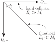
Figure 1: Illustration of the various regions of validity of our parametrization. As seen from, eq. (21) the condition $p_{i}\cdot Q_{i,s}\ll p_{i}\cdot n_{i,s}$ is fulfilled if either both $Q_{i+}$ and $Q_{i-}$ are small (the genuinely soft region) or if $E_{i}\gg M_{i}$ and $Q_{i-}\rightarrow 0$ (the hard collinear region) or if $E_{i}\ll M_{i}$ and $Q_{i-}\rightarrow-Q_{i+}$ (the threshold region).

Appendix C Propagators and external wave functions

An important ingredient to our factorization formula is to demonstrate, subject to the kinematic parametrization above, that

$$\sum_{n=0}^{\infty}\left(\frac{{\mathbf{P}}(q_{i}+K_{i,s},M_{i})}{(q_{i}+K_{i,s})^{2}-\tilde{M}_{R,i}^{2}}{\mathbf{\Sigma}}(q_{i}+K_{i,s})\right)^{n}\frac{{\mathbf{P}}(q_{i}+K_{i,s},M_{i})}{(q_{i}+K_{i,s})^{2}-\tilde{M}_{R,i}^{2}}=\frac{1}{2p_{i}\cdot Q_{i,s}}\frac{\Psi(\Lambda p_{i},M_{i})\bar{\Psi}(\Lambda p_{i},M_{i})}{1-\Sigma^{\prime}(M_{i}^{2})}+{\cal O}(\lambda)\ ,$$ (22)

where the derivative of the (physical part of the) self-energy $\Sigma(p^{2})$ (or, accordingly the transverse self-energy at vanishing $k^{2}$ for a massless boson) provides the proper wave function renormalization for the amplitude we factor to. To illustrate this let us first consider Goldstone bosons in an $R_{\xi}$ gauge, with a free propagator $i/(k^{2}-\xi\tilde{M}_{R,i}^{2})$, where $\tilde{M}_{R,i}^{2}=M_{R,i}^{2}+iM_{R,i}\Gamma_{R,i}$ in a complex mass scheme Denner and Dittmaier (2006); Denner and Lang (2015), and the introduction of $\Gamma_{R,i}$ needs to be added back as additional insertions of two-point functions. This does not provide any change to our main argument. The propagators of the physical scalar can be obtained by putting $\xi=1$. If the scalar has a one-particle irreducible two-point function $-i\Sigma_{S}(k^{2})$, the resummed propagator is

$$\frac{1}{(q_{i}+K_{i,s})^{2}-\xi\tilde{M}_{R,i}^{2}-\Sigma_{S}((q_{i}+K_{i,s})^{2})}=\left\{\begin{array}[]{cc}\frac{1}{2p_{i}\cdot Q_{i,s}}\frac{1}{1-\Sigma^{\prime}(M_{i}^{2})}+{\cal O}(\lambda)&\xi=1\text{ and }\Sigma_{S}(k^{2})=\Sigma(k^{2})\\ {\cal O}(\lambda)&\text{ otherwise }\end{array}\right.$$ (23)

where the physical and renormalized (complex) mass relate as $M_{i}^{2}=\tilde{M}_{R,i}^{2}+\Sigma(M_{i}^{2})$ for the boson in question. Thus depending on how the unphysical scalar’s self energy and the gauge parameter relate to each other, the scalars will contribute at leading power along with their related vector bosons, or not. We will investigate this in more detail in the future. The simplest non-scalar case to consider is that of a massive gauge boson. In an $R_{\xi}$ gauge their numerator reads

$$V^{\mu\nu}(q_{i}+K_{i,s},M_{i})=-\eta^{\mu\nu}+(1-\xi)\frac{(q_{i}+K_{i,s})^{\mu}(q_{i}+K_{i,s})^{\nu}}{(q_{i}+K_{i,s})^{2}-\xi M_{i}^{2}}\;.$$ (24)

Using the momentum parametrization eq. (3) we have

$$V^{\mu\nu}(q_{i}+K_{i,s},M_{i})=-\eta^{\mu\nu}-\alpha^{2}(1-\xi)\frac{(\Lambda p_{i})^{\mu}(\Lambda p_{i})^{\nu}}{2p_{i}\cdot Q_{i,s}+(1-\xi)M_{i}^{2}}=\sum_{\lambda}\epsilon_{\lambda,M}^{\mu}(\Lambda p_{i},M_{i})\epsilon_{\lambda,M}^{*,\nu}(\Lambda p_{i},M_{i})+{\cal O}(\lambda)$$ (25)

where the physical polarization sum is $\sum_{\lambda}\epsilon_{\lambda,M}^{\mu}(p_{i},M_{i})\epsilon_{\lambda,M}^{*,\nu}(p_{i},M_{i})=-\eta^{\mu\nu}+p_{i}^{\mu}p_{i}^{\nu}/M_{i}^{2}$. At tree level and $\xi=1$ this would not hold, but in this case the Goldstones would contribute, as shown above. For $\xi\neq 1$ we obtain the physical polarization sum, and the Goldstones would not contribute. The summed propagator is more complicated, however we still find that the above relation holds with the expected additional factor of the (complex) transverse self-energy of the respective boson, as claimed at the beginning of this section. For Fermions the propagator numerator is linear in the momentum and thus they trivially satisfy our constraints at leading power. The last complicated case is that of a massless gauge boson in physical gauge, for which we observe that

$$d^{\mu\nu}(q,n)=-\eta^{\mu\nu}+\frac{q^{\mu}n^{\nu}+n^{\mu}q^{\nu}}{n\cdot q}$$ (26)

which clearly satisfies

$$d^{\mu\nu}(q_{i}+K_{i,s},n)=d^{\mu\nu}(\Lambda p_{i})+{\cal O}(\lambda)=\sum_{\lambda}\epsilon_{\lambda}^{\mu}(\Lambda p_{i},n)\epsilon_{\lambda}^{*,\nu}(\Lambda p_{i},n)+{\cal O}(\lambda)$$ (27)

where $\epsilon(q,n)$ are the physical transverse polarization vectors satisfying $\epsilon(q,n)\cdot q=\epsilon\cdot n=0$ and $\epsilon_{\lambda}(q,n)\cdot\epsilon_{\sigma}(q,n)=-\delta_{\lambda\sigma}$. For a full propagator we get the usual renormalization factor $1/(1-\Sigma_{T}(0))$ where $\Sigma_{T}$ is the transverse part of the self energy, and the part which is longitudinal to the gauge vector is again only contributing at subleading power.

In total, this allows us to write, at leading power,

$$\left(\prod_{i\notin h_{s}}\bar{\Psi}_{f_{i}}(q_{i},m_{i})\right)\left(\prod_{i\in h_{s}}\frac{{\mathbf{P}}_{f^{\prime}_{i}}(q_{i}+K_{i,s},M_{i})}{(q_{i}+K_{i,s})^{2}-M_{i}^{2}}\right)|{\cal M}_{\{f_{i}^{\prime}\}_{n}}(\{P_{i}\}_{n})\rangle=\\ \left(\prod_{i\in h_{s}}\frac{\Psi_{f^{\prime}_{i}}(\Lambda p_{i},M_{i})}{2p_{i}\cdot Q_{i,s}}\right)\times\left(\prod_{i}\bar{\Psi}_{f^{\prime}_{i}}(p_{i},M_{i})|{\cal M}_{\{f_{i}^{\prime}\}_{n}}(\{p_{i}\}_{n})\rangle\right)+{\cal O}(\lambda^{-\#h_{s}+1})\ ,$$ (28)

where $\#h_{s}$ is the number of hard off-shell legs interacting with unresolved partons. This completes the derivation of our general factorization formula.

Appendix D The flow picture for the gauge groups

In this section we present more details on how the flow picture usually employed for QCD can be generalized to the electroweak SM. Effectively, we can distinguish different flow types by their isospin component, where it is understood that no summation is performed, i.e. closed loops do not evaluate to $\delta_{i}^{i}$ the dimension of the gauge group. Amplitudes can then be organized within a basis in which we distinguish connections which flip isospin components, and those which connect the same components. The former would e.g. originate from $W$ bosons coupling to fermions, and the latter would originate from neutral gauge bosons coupling to fermions. Though the picture is more general and also accordingly includes (charged) Goldstone bosons, as well as ghost contributions. Amplitudes which do not involve fermions can be decomposed accordingly, and just like purely gluonic amplitudes in the color flow basis exhibit more flow lines than actual particles. In Fig. 2 we give a few examples of flow patterns, and the lines we associate to isospin flipping ($\sim\tau^{\pm}$) exchanges, as well as to the diagonal exchanges.

Figure 2: Examples of isospin flows. An amplitude can be decomposed into a basis composed of the leftmost four flows, and exchanges of electroweak bosons will act as indicated. We have highlighted the physical Bosons associated to these lines, though the same line patterns apply to the respective Goldstone bosons and ghosts.

Appendix E Chirality-flow basis and effect of exchange

We here prove the statement that all chirality-flow structures can be recast only to the structures in eq. (14). We also schematically derive the decomposition of structures with up to six momentum dots which can appear in intermediate steps.

First, we note that the usage of $\langle i\,j\rangle,[i\,j]$; $p_{\mu}[i\,|\sigma^{\mu}|j\rangle,p_{\mu}\langle i\,|\bar{\sigma}^{\mu}|j]$ and $A_{\mu\nu}\langle i\,|\bar{\sigma}^{[\mu}\sigma^{\nu]}|j\rangle$, $A_{\mu\nu}\langle i\,|\sigma^{[\mu}\bar{\sigma}^{\nu]}|j]$ for some antisymmetric tensor $A^{\mu\nu}$, is equivalent to the decomposition of products of $\gamma$-matrices into $1$ and $\gamma^{5}$ (via the decomposition into left and right chiral states); $\gamma^{\mu},\;\gamma^{5}\gamma^{\mu}$ and $[\gamma^{\mu},\gamma^{\nu}]$ respectively.

In principle this is in itself a proof that these are the structures to anticipate. Nevertheless we will explicitly prove that the action of gauge boson exchange, starting from any of these structures, will result in linear combinations of the same spanning structures. That this holds for exchange of fermions and scalars then follows trivially. We start with considering the simplest case when two momentum dots, for example coming from the fermion propagators (slashed momenta) arising by photon exchange, are attached to the same chirality-flow line. Using the chirality-flow Feynman rules from Lifson et al. (2020), we obtain

$$\raisebox{-30.0pt}{ \includegraphics[scale={0.4}]{jaxodraw/chirality-flow-photon-exchange-1-decomp} },$$ (29)

i.e. the partners $i^{\prime}$ and $j^{\prime}$ (originally connected to $i$ and $j$ respectively) become chirality-flow connected, whereas $i$ and $j$ instead becomes connected to each other. To decompose the two momentum dots into our basis, we use the identity

$$\sigma^{\mu}\bar{\sigma}^{\nu}=g^{\mu\nu}+\frac{1}{2}(\sigma^{\mu}\bar{\sigma}^{\nu}-\sigma^{\nu}\bar{\sigma}^{\mu})\;.$$ (30)

Contracting with external momenta $p_{1}$ and $p_{2}$, and sandwiching between external spinors this gives

$$\underbrace{[i\,|p_{1\mu}p_{2\nu}\sigma^{\mu}\bar{\sigma}^{\nu}|j]}_{\equiv\raisebox{-5.69046pt}{\includegraphics[scale={0.4}]{jaxodraw/2-mom-dot-LHS}}}=p_{1}\cdot p_{2}\underbrace{[i\,j]}_{\quad\equiv\raisebox{-5.69046pt}{\includegraphics[scale={0.4}]{jaxodraw/2-mom-dot-RHS1}}}+\hskip 11.38092pt\underbrace{[i\,|p_{1\mu}p_{2\nu}\frac{1}{2}(\sigma^{\mu}\bar{\sigma}^{\nu}-\sigma^{\nu}\bar{\sigma}^{\mu})|j]}_{\equiv\raisebox{-11.38092pt}{\includegraphics[scale={0.4}]{jaxodraw/2-mom-dot-RHS2}}}\;.$$ (31)

(applied to $i^{\prime}$ and $j^{\prime}$). We remark that it is the antisymmetric part of $p_{1\mu}p_{2\nu}$, $\frac{1}{2}(p_{1\mu}p_{2\nu}-p_{1\nu}p_{2\mu})$ that survives the contraction; more generally, we find an antisymmetric rank-2 tensor contracted with $\frac{1}{2}(\sigma^{\mu}\bar{\sigma}^{\nu}-\sigma^{\nu}\bar{\sigma}^{\mu})$.

Exploring the effect on the basis vector we obtain

$$\raisebox{-22.0pt}{\includegraphics[scale={0.4}]{jaxodraw/2-delta-initial-flow}}\rightarrow\raisebox{-24.0pt}{\includegraphics[scale={0.4}]{jaxodraw/chirality-flow-photon-exchange-1-new-flow}}=\;p_{1}\cdot p_{2}\raisebox{-22.0pt}{\includegraphics[scale={0.4}]{jaxodraw/2-delta-RHS1}}+A_{12}\raisebox{-22.0pt}{\includegraphics[scale={0.4}]{jaxodraw/2-delta-RHS2}}\;\text{with}\;(A_{12})_{\mu\nu}=\frac{1}{2}(p_{1\mu}p_{2\nu}-p_{1\nu}p_{2\mu})\;,$$ (32)

in the typical case that $i$ and $j$ are not chirality-flow connected to each other. If they are, we find

$$\rightarrow p_{1}\cdot p_{2}\raisebox{-17.0pt}{\includegraphics[scale={0.4}]{jaxodraw/1-delta-RHS1}}\;=2p_{1}\cdot p_{2}\raisebox{-10.0pt}{\includegraphics[scale={0.4}]{jaxodraw/1-delta-initial-flow}}\;,$$ (33)

i.e. we get back the chirality flow that we start with.

When describing the effect of spin-1 exchange, we also encounter structures with three momentum dots, for example while exchanging a photon between two fermions ($i$ and $j$) which are chirality-flow connected with partners ($i^{\prime}$ and $j^{\prime}$), in one case directly and in the other with a single momentum-dot in-between

$$\raisebox{-32.0pt}{\includegraphics[scale={0.4}]{jaxodraw/chirality-flow-photon-exchange-3dot}}.$$ (34)

The line with three bullets represents the contraction $p_{1\mu}p_{2\nu}p_{3\rho}[i^{\prime}\,|\sigma^{\mu}\bar{\sigma}^{\nu}\sigma^{\rho}|j^{\prime}\rangle$ for the four-vectors $p_{1},\,p_{2}$ and $p_{3}$ associated with the momentum-dots. To decompose this structure, we contract $\sigma^{\mu}\bar{\sigma}^{\nu}\sigma^{\rho}$ with $g_{\mu\nu},g_{\mu\rho},g_{\nu\rho}$ and $\epsilon_{\mu\nu\rho\alpha}$, giving a system of four equations and four unknowns with solution

$$\sigma^{\mu}\bar{\sigma}^{\nu}\sigma^{\rho}=g^{\mu\nu}\sigma^{\rho}-g^{\mu\rho}\sigma^{\nu}+g^{\nu\rho}\sigma^{\mu}+i\epsilon^{\mu\nu\rho}_{\;\;\;\;\;\alpha}\sigma^{\alpha}\;,$$ (35)

corresponding to

$$p_{1\mu}p_{2\nu}p_{3\rho}[k\,|\sigma^{\mu}\bar{\sigma}^{\nu}\sigma^{\rho}|j\rangle=p_{1}\cdot p_{2}\,p_{3\rho}[k\,|\sigma^{\rho}|j\rangle-p_{1}\cdot p_{3}\,p_{2\rho}[k\,|\sigma^{\rho}|j\rangle+p_{2}\cdot p_{3}\,p_{1\rho}[k\,|\sigma^{\rho}|j\rangle+i\underbrace{p_{1\mu}p_{2\nu}p_{3\rho}\epsilon^{\mu\nu\rho}_{\;\;\;\;\;\alpha}}_{p_{123\,\alpha}}[k\,|\sigma^{\alpha}|j\rangle\;,$$ (36)

or in the momentum-dot notation (for general $[k|$ and $|j\rangle$)

$$= p_{1}\cdot p_{2}\;\raisebox{-3.0pt}{\includegraphics[scale={0.4}]{jaxodraw/3-mom-dot-RHS1}}-p_{1}\cdot p_{3}\;\raisebox{-3.0pt}{\includegraphics[scale={0.4}]{jaxodraw/3-mom-dot-RHS2}}+p_{2}\cdot p_{3}\;\raisebox{-3.0pt}{\includegraphics[scale={0.4}]{jaxodraw/3-mom-dot-RHS3}}+i\;\raisebox{-3.0pt}{\includegraphics[scale={0.4}]{jaxodraw/3-mom-dot-RHS4}}$$ (37)

$$= \;\raisebox{-3.0pt}{\includegraphics[scale={0.4}]{jaxodraw/3-mom-dot-RHSRHS}}\quad\text{for}\quad P_{123}\equiv p_{1}\cdot p_{2}\,p_{3}-p_{1}\cdot p_{3}\,p_{2}+p_{2}\cdot p_{3}\,p_{1}+ip_{123}\;.$$ (38)

This means that we retrieve the structure of a single momentum-dot for some momentum $P_{123}$.

For the action of a momentum-dot on our basic building blocks, the basis vectors, eq. (14), we find by antisymmetrizing

$$\raisebox{-3.0pt}{\includegraphics[scale={0.4}]{jaxodraw/box-dot-LHS1}}=-p_{1}\cdot p_{3}\;\raisebox{-3.0pt}{\includegraphics[scale={0.4}]{jaxodraw/3-mom-dot-RHS2}}+p_{2}\cdot p_{3}\;\raisebox{-3.0pt}{\includegraphics[scale={0.4}]{jaxodraw/3-mom-dot-RHS3}}+i\;\raisebox{-3.0pt}{\includegraphics[scale={0.4}]{jaxodraw/3-mom-dot-RHS4}}.$$ (39)

In the general case, the contraction to the left is with a general antisymmetric rank-2 tensor $(A_{12})_{\mu_{1}\mu_{2}}$. In this case, defining

$$P_{[[1,2],3]\mu}=2(A_{12})_{\mu\nu}p_{3}^{\nu}+i(A_{12})_{\mu_{1}\mu_{2}}p_{3\mu_{3}}{\epsilon^{\mu_{1}\mu_{2}\mu_{3}}}_{\mu}$$ (40)

the decomposition reads

$$\raisebox{-3.0pt}{\includegraphics[scale={0.4}]{jaxodraw/box-dot-LHS}}=\;\raisebox{-3.0pt}{\includegraphics[scale={0.4}]{jaxodraw/box-dot-RHSv2}}.$$ (41)

The next structures to consider are those with a total of four contractions, either of form (where the middle two dots come from a fermion propagator, and the outermost dots from the initial chirality flows containing one momentum dot each), of form (from one initial chirality flow of type , one or two momentum dots from a propagator, and (if one) the other from the initial chirality flow of the other involved fermion), or of form (from an initial state of two boxes contracted with the mass term in the propagator).

For this decomposition, we first explore the antisymmetric part . Exploiting symmetries and fixing constants, this can be decomposed into

$$\raisebox{-4.0pt}{\includegraphics[scale={0.4}]{jaxodraw/box-box}}=\left[-2(A_{12})_{\mu_{1}\mu_{2}}(A_{34})^{\mu_{1}\mu_{2}}+i\epsilon^{\mu_{1}\mu_{2}\mu_{3}\mu_{4}}(A_{12})_{\mu_{1}\mu_{2}}(A_{34})_{\mu_{3}\mu_{4}}\right]\raisebox{-3.0pt}{\includegraphics[scale={0.4}]{jaxodraw/2-mom-dot-RHS1}}+\raisebox{-4.0pt}{\includegraphics[scale={0.4}]{jaxodraw/box-box-RHS2}}$$ (42)

where

$$A^{\prime}_{[[1,2],[3,4]]\,\mu\nu}=2\left((A_{12})_{\mu\eta}{(A_{34})^{\eta}}_{\nu}-(A_{12})_{\nu\eta}{(A_{34})^{\eta}}_{\mu}\right)$$ (43)

is made manifestly antisymmetric since only the antisymmetric part survives the contraction. The result in eq. (42), along with eq. (31) and (and versions where dotted and undotted lines switch role) completes the set of basic calculation rules needed to decompose any number of momentum dots and boxes in a sequence.

For example, using eq. (31) along with eq. (42) the decompositions of as well as are straightforwardly obtained,

$$= p_{3}\cdot p_{4}\raisebox{-4.0pt}{{\includegraphics[scale={0.4}]{jaxodraw/box-dot-dot-RHS1}}}+\raisebox{-4.0pt}{\includegraphics[scale={0.4}]{jaxodraw/box-dot-dot-RHS2}}$$ (44)

$$= p_{1}\cdot p_{2}\,p_{3}\cdot p_{4}\raisebox{-3.0pt}{\includegraphics[scale={0.4}]{jaxodraw/4-mom-dot-RHS0}}+p_{3}\cdot p_{4}\raisebox{-4.0pt}{\includegraphics[scale={0.4}]{jaxodraw/4-mom-dot-RHS1}}+p_{1}\cdot p_{2}\raisebox{-4.0pt}{\includegraphics[scale={0.4}]{jaxodraw/4-mom-dot-RHS2}}+\raisebox{-4.0pt}{\includegraphics[scale={0.4}]{jaxodraw/4-mom-dot-RHS3}}$$

where the double box structures may be expanded out using eqs. (42) and (43).

Similarly structures with in total five index contractions (, , as well as versions with dotted and undotted lines interchanged, and versions with arrows swapped) and 6 contractions (only and a versions with dotted and undotted lines interchanged) can be obtained.

In this way, the chirality-flow state obtained after several exchanges can iteratively be built up, and we obtain a chirality-flow decomposition analogous to the color-flow decomposition, but with the difference that there are three types of “flows” connecting partons, and that particles and anti-particles enter on equal footing.

To illustrate this we consider consider an example of intermediate complexity

$$\raisebox{-22.0pt}{\includegraphics[scale={0.4}]{jaxodraw/chirality-flow-photon-exchange-box-dot-dot}}\;,$$ (45)

which, at the level of the basis vectors has the effect,

$$\rightarrow \left(-2(A_{12})_{\mu_{1}\mu_{2}}(A_{34})^{\mu_{1}\mu_{2}}+i\epsilon^{\mu_{1}\mu_{2}\mu_{3}\mu_{4}}(A_{12})_{\mu_{1}\mu_{2}}(A_{34})_{\mu_{3}\mu_{4}}\right)\raisebox{-22.0pt}{\includegraphics[scale={0.4}]{jaxodraw/chirality-flow-photon-exchange-box-dot-dot-RHS1}}\;+A^{\prime}\raisebox{-22.0pt}{\includegraphics[scale={0.4}]{jaxodraw/chirality-flow-photon-exchange-box-dot-dot-RHS2}}\;$$

with $$\quad A_{34\,\mu\nu}=\frac{1}{2}(p_{3\mu}p_{4\nu}-p_{3\nu}p_{4\mu})\quad\text{and}\quad A^{\prime}_{\mu\nu}=p_{3}\cdot p_{4}A_{12\mu\nu}+2\left((A_{12})_{\mu\eta}{(A_{34})^{\eta}}_{\nu}-(A_{12})_{\nu\eta}{(A_{34})^{\eta}}_{\mu}\right)$$

as seen by expanding out eqs. (42) and (43) in eq. (E).

In the light of the above description, combined with the chirality-flow Standard Model Feynman rules Alnefjord et al. (2021), it is clear that scalar exchange, involving no chirality-flow line, does not change the chirality flow (but alters the involved momenta). Fermion exchange adds one (from the slashed momentum in the propagator) or zero (from a potential mass term) momentum dots to existing chirality-flow structures Alnefjord et al. (2021). For the mass term, the line type of the fermion line is left unchanged, but the chirality-flow structure will change since (for example) chirality-flow lines which are not originally connected may become connected. External massive fermions have to be decomposed into left- and right-chiral states, as for example in Alnefjord et al. (2021).

For the non-abelian vertices, we recall that they may be decomposed into momentum-dot structures Lifson et al. (2020); Alnefjord et al. (2021), and therefore do not add to the number of possible chirality-flow structures. (If a $W^{\pm}$, instead of a photon, is exchanged, the chiral structure is rather simplified.) For external gauge bosons, we note that positive and negative helicity spin-1 particles appear as one dotted and one undotted line with opposite directions, whereas the longitudinal polarization of a massive vector boson can be expressed in terms of a momentum dot Alnefjord et al. (2021). External gauge bosons do, however, somewhat complicate the description, since they may add a dependence on a reference gauge vector (which is unphysical in the massless case, and related to the direction in which spin is measured in the massive).

In view of the above, we conclude that the flow basis in eq. (14) is applicable to resummation of all chiral structures following after exchange of any known particle. This is the analogue for the color-flow basis.

References

- Catani and Grazzini (2000) S. Catani and M. Grazzini, Nucl. Phys. B 570, 287 (2000), arXiv:hep-ph/9908523 .
- Forshaw et al. (2020) J. R. Forshaw, J. Holguin, and S. Plätzer, JHEP 09, 014 (2020), arXiv:2003.06400 [hep-ph] .
- Kidonakis et al. (1998) N. Kidonakis, G. Oderda, and G. Sterman, Nucl. Phys. B531, 365 (1998), hep-ph/9803241 .
- Contopanagos et al. (1997) H. Contopanagos, E. Laenen, and G. Sterman, Nuclear Physics B 484, 303 (1997).
- Oderda (2000) G. Oderda, Phys. Rev. D 61, 014004 (2000), arXiv:hep-ph/9903240 .
- Sjodahl (2009) M. Sjodahl, JHEP 09, 087 (2009), arXiv:0906.1121 [hep-ph] .
- Plätzer (2014) S. Plätzer, Eur. Phys. J. C74, 2907 (2014), arXiv:1312.2448 [hep-ph] .
- Ángeles Martinez et al. (2018) R. Ángeles Martinez, M. De Angelis, J. R. Forshaw, S. Plätzer, and M. H. Seymour, JHEP 05, 044 (2018), arXiv:1802.08531 [hep-ph] .
- De Angelis et al. (2021) M. De Angelis, J. R. Forshaw, and S. Plätzer, Phys. Rev. Lett. 126, 112001 (2021), arXiv:2007.09648 [hep-ph] .
- Plätzer and Ruffa (2021) S. Plätzer and I. Ruffa, JHEP 06, 007 (2021), arXiv:2012.15215 [hep-ph] .
- Forshaw et al. (2019) J. R. Forshaw, J. Holguin, and S. Plätzer, JHEP 08, 145 (2019), arXiv:1905.08686 [hep-ph] .
- Löschner et al. (2021) M. Löschner, S. Plätzer, and E. S. Dore, (2021), arXiv:2112.14454 [hep-ph] .
- Ciafaloni and Comelli (1999) P. Ciafaloni and D. Comelli, Phys. Lett. B 446, 278 (1999), arXiv:hep-ph/9809321 .
- Denner and Pozzorini (2001a) A. Denner and S. Pozzorini, Eur. Phys. J. C 18, 461 (2001a), arXiv:hep-ph/0010201 .
- Denner and Pozzorini (2001b) A. Denner and S. Pozzorini, Eur. Phys. J. C 21, 63 (2001b), arXiv:hep-ph/0104127 .
- Ciafaloni and Comelli (2005) P. Ciafaloni and D. Comelli, JHEP 11, 022 (2005), arXiv:hep-ph/0505047 .
- Chiu et al. (2008) J.-y. Chiu, F. Golf, R. Kelley, and A. V. Manohar, Phys. Rev. Lett. 100, 021802 (2008), arXiv:0709.2377 [hep-ph] .
- Manohar and Waalewijn (2018) A. V. Manohar and W. J. Waalewijn, JHEP 08, 137 (2018), arXiv:1802.08687 [hep-ph] .
- Kleiss and Verheyen (2020) R. Kleiss and R. Verheyen, Eur. Phys. J. C 80, 980 (2020), arXiv:2002.09248 [hep-ph] .
- Masouminia and Richardson (2021) M. R. Masouminia and P. Richardson, (2021), arXiv:2108.10817 [hep-ph] .
- Brooks et al. (2021) H. Brooks, P. Skands, and R. Verheyen, (2021), arXiv:2108.10786 [hep-ph] .
- Chen et al. (2017) J. Chen, T. Han, and B. Tweedie, JHEP 11, 093 (2017), arXiv:1611.00788 [hep-ph] .
- Bauer et al. (2017) C. W. Bauer, N. Ferland, and B. R. Webber, JHEP 08, 036 (2017), arXiv:1703.08562 [hep-ph] .
- Bauer et al. (2018) C. W. Bauer, D. Provasoli, and B. R. Webber, JHEP 11, 030 (2018), arXiv:1806.10157 [hep-ph] .
- Plätzer (2022) S. Plätzer, “Colour Evolution and Infrared Physics,” to appear (2022).
- Manohar et al. (2015) A. Manohar, B. Shotwell, C. Bauer, and S. Turczyk, Phys. Lett. B 740, 179 (2015), arXiv:1409.1918 [hep-ph] .
- Reiner and Maas (2022) F. Reiner and A. Maas, PoS EPS-HEP2021, 449 (2022), arXiv:2110.07312 [hep-ph] .
- Denner and Dittmaier (2006) A. Denner and S. Dittmaier, Nucl. Phys. B Proc. Suppl. 160, 22 (2006), arXiv:hep-ph/0605312 .
- Denner and Lang (2015) A. Denner and J.-N. Lang, Eur. Phys. J. C 75, 377 (2015), arXiv:1406.6280 [hep-ph] .
- Frixione and Webber (2021) S. Frixione and B. R. Webber, JHEP 11, 045 (2021), arXiv:2106.13471 [hep-ph] .
- Forshaw et al. (2021) J. R. Forshaw, J. Holguin, and S. Plätzer, (2021), arXiv:2112.13124 [hep-ph] .
- Lifson et al. (2020) A. Lifson, C. Reuschle, and M. Sjodahl, Eur. Phys. J. C 80, 1006 (2020), arXiv:2003.05877 [hep-ph] .
- Alnefjord et al. (2021) J. Alnefjord, A. Lifson, C. Reuschle, and M. Sjodahl, Eur. Phys. J. C 81, 371 (2021), arXiv:2011.10075 [hep-ph] .
- Lifson et al. (2022) A. Lifson, M. Sjodahl, and Z. Wettersten, (2022), arXiv:2203.13618 [hep-ph] .