An odd-frequency Cooper pair around a magnetic impurity

Abstract

The Yu-Shiba-Rusinov (YSR) state appears as a bound state of a quasiparticle at a magnetic atom embedded in a superconductor. We discuss why the YSR state has energy below the superconducting gap and why the pair potential changes the sign at the magnetic atom. Although a magnetic atom in a superconductor has been considered as a pair breaker since 1960s, we propose an alternative physical picture to explain these reasons. The analytical expression of the Green’s function indicates that a magnetic atom converts a spin-singlet $s$-wave Cooper pair into odd-frequency Cooper pairs rather than breaking it and that the odd-frequency pairing correlations coexist with the YSR states below the gap. The relationships among the free-energy density, the amplitudes of pairing correlation functions, and the sign change of the pair potential at a magnetic impurity are discussed utilizing the self-consistent solution of the Eilenberger equation. We conclude that the sign change of the pair potential happens only when the amplitudes of odd-frequency pairing correlations are dominant at the magnetic impurity. In the presence of the local $\pi$-phase shift in the pair potential, odd-frequency pairs can decrease the free-energy density there because their response to a magnetic field is paramagnetic.

I Introduction

The Yu-Shiba-Rusinov (YSR) state [1, 2, 3] is a bound state around a magnetic impurity embedded in a superconductor and is considered to appear as a result of breaking a spin-singlet Cooper pair by the magnetic moment. Superconducting junctions with the YSR states have been attracting renewed attention as a possible platform for quantum computer architectures. Actually it is known that a chain of magnetic nanoparticles on an $s$-wave superconductor accommodates Majorana fermions at its ends [4, 5, 6]. Controlling the superconducting subgap state is a necessary element of future quantum technology [7, 8, 9].

A spin-singlet Cooper pair is formed by two electrons which are time-reversal partner to each other. Thus a magnetic impurity (a defect breaking time-reversal symmetry) acts as a pair-breaker. Indeed it is widely accepted that magnetic impurities drastically suppress the superconducting transition temperature $T_{c}$ [10, 11]. Although the formation of YSR state was pointed out in 1960s, there are three unsolved issues as listed below. (i) This conventional simple picture does not explain why magnetic impurity generates the YSR states below the gap. (ii) A strong magnetic impurity changes the sign of the pair potential around the impurity site [12, 13, 14, 15]. As briefly mentioned in a review paper [16], there is no convincing explanation for the local $\pi$-phase shift even now. (iii) It has been unclear the relation between the appearance of the YSR states and the suppression of $T_{c}$. In this paper, we will show that the existence of odd-frequency Cooper pairs around the magnetic impurity provides satisfactory explanation to these issues.

The odd-frequency Cooper pairing is a concept which was introduced by Berezinskii [17] to explain the superfluidity in ³He. Although there has been much theoretical work on odd-frequency superconducting states in bulk systems since 1990s [18, 19, 20, 21, 22, 23, 24, 25], experimental evidence is still lacking. One of authors showed that the spatially uniform odd-frequency superconducting order is impossible in single-band metals [26]. However, it turns out that the odd-frequency spin-triplet $s$-wave triplet state can be realized as an induced subdominant pairing correlation in a rather conventional system consisting of a spin-singlet $s$-wave superconductor and a ferromagnet [27]. Induced odd-frequency pairing correlations have been discussed in connection with a subgap quasiparticle appearing at a surface of unconventional superconductors [28, 29, 30, 31, 32], a vortex core [33, 34], and an edge of a Majorana nanowire [35]. In superconductors having internal degrees of freedom (e.g. sublattices, multi-orbital, and multi-band), a quasiparticle on the Bogoliubov Fermi surface [36] accompanies an odd-frequency Cooper pair [37]. Although the odd-frequency pairing correlations around a magnetic impurity were pointed out by recent studies [38, 39], physical phenomena unique to an odd-frequency Cooper pair have not been discussed yet. The most important property of odd-frequency Cooper pairs is that they exhibit a paramagnetic response to an external magnetic field [40, 41, 42, 43]. When the amplitude of an odd-frequency pair is dominant at some place in a superconductor, the spatial gradient in the superconducting phase decreases the free-energy there. Indeed, two of authors showed that the magnetic response of a small unconventional superconductor can be paramagnetic at a low temperature [42]. We summarize physical consequences of paramagnetic Cooper pairs in Appendix A.

In this paper, we calculate the Green’s function around a magnetic impurity in a spin-singlet $s$-wave superconductor both analytically and numerically. The analytical expression of the anomalous Green’s function shows that the magnetic impurity converts a spin-singlet $s$-wave Cooper pair into an odd-frequency Cooper pair. The direct comparison between the normal and the anomalous Green’s functions explains well the coexistence of such an odd-frequency pair and a quasiparticle at the YSR states. Thus the formation of YSR states below the gap is a natural consequence of appearing of an odd-frequency pair. As a result of the symmetry conversion of a Cooper pair, the amplitude of the spin-singlet $s$-wave pairing correlation decreases down to zero and changes the sign with the increase of the amplitude of magnetic moment. To explain why the pair potential changes the sign around a magnetic impurity, we analyze the free-energy density and the pairing correlation function around the magnetic impurity by solving the Eilenberger equation [44, 45] numerically. The results show that the free-energy density at a magnetic impurity can be larger than that in the normal state. Such an unusual local state is possible only in a inhomogeneous superconductor. Odd-frequency Cooper pairs increase the free-energy density because they are thermodynamically unstable under the spatially uniform pair potential. We also show that the free-energy density at the impurity is decreased by the $\pi$-phase shift in the pair potential when odd-frequency Cooper pairs stay more dominantly than even-frequency pairs. The paramagnetic response of odd-frequency pairs explains naturally the close relationships among the appearance of an odd-frequency Cooper pair, the local $\pi$-phase shift in the pair potential, and the instability of superconducting state around the impurity. As an extension of the main conclusions, we also discuss the decrease of transition temperature $T_{c}$ in the presence of a number of magnetic impurities.

This paper is organized as follows. In Sec. II, we summarize the pairing correlations around a magnetic impurity embedded in a superconductor in one-dimension. In Sec. III, we display numerical results of the pair potential, the local density of states, the pairing correlations, and the free-energy density. We explain why the appearance of odd-frequency pairs decreases $T_{c}$ in Sec. IV. The conclusion is given in Sec. V. Throughout this paper, we use the system of units $\hbar=k_{B}=c=1$, where $k_{B}$ is the Boltzmann constant and $c$ is speed of light.

II Cooper pairs around a magnetic impurity

Let us consider a spin-singlet $s$-wave superconductor in one-dimension where a magnetic impurity is embedded at $x=0$. The Bogoliubov-de Gennes (BdG) Hamiltonian of a superconductor is given by

$$\check{H}_{\mathrm{BdG}}(x)= \left[\begin{array}[]{cc}\xi_{x}&\Delta i\hat{\sigma}_{2}e^{i\varphi}\\ \Delta(-i)\hat{\sigma}_{2}e^{-i\varphi}&-\xi_{x}^{\ast}\end{array}\right]+\check{V}(x),$$ (3)

$$\xi_{x}= -\frac{1}{2m}\frac{d^{2}}{dx^{2}}-\epsilon_{F},$$ (4)

where $\Delta$ is the uniform pair potential in spin-singlet $s$-wave symmetry, $\epsilon_{F}$ is the Fermi energy, $\check{V}$ represents the impurity potential, and $\hat{\sigma}_{j}$ for $j=1-3$ is the Pauli matrix in spin space. The potential of a paramagnetic impurity at $x=0$ is described by

$$\check{V}(x)= \left[\begin{array}[]{cc}\bm{V}\cdot\hat{\bm{\sigma}}&0\\ 0&-\bm{V}\cdot\hat{\bm{\sigma}}^{\ast}\end{array}\right]\,\delta(x).$$ (7)

The Gor’kov equation reads,

$$\left[i\omega_{n}-\check{H}_{\mathrm{BdG}}(x)\right]\check{\mathcal{G}}(x-x^{\prime})=\check{1}\,\delta(x-x^{\prime}),$$ (8)

where $\omega_{n}=(2n+1)\pi T$ is the Matsubara frequency with $n$ and $T$ being an integer number and a temperature, respectively. The Green’s function has a structure

$$\check{\mathcal{G}}(x,x^{\prime})=\left[\begin{array}[]{cc}\hat{g}(x,x^{\prime})&\hat{f}(x,x^{\prime})\\ -\hat{f}^{\ast}(x,x^{\prime})&-\hat{g}^{\ast}(x,x^{\prime})\end{array}\right],$$ (11)

because of particle-hole symmetry in the BdG Hamiltonian. As shown in Appendix B, the Green’s function in the presence of an impurity can be calculated exactly. The normal Green’s function is shown in Eq. (89) in Appendix B. The density of states are calculated from the normal Green’s function in the retarded causality

$$N(x,\epsilon)=-\frac{1}{4\pi}\mathrm{Im}\,\mathrm{Tr}\left[\check{\mathcal{G}}^{R}_{\epsilon}(x,x)\right]=-\frac{1}{4\pi}\mathrm{Im}\,\mathrm{Tr}\left[\hat{g}^{R}_{\epsilon}(x,x)-(\hat{g}^{R}_{\epsilon})^{\ast}(x,x)\right],\quad\check{\mathcal{G}}^{R}_{\epsilon}(x,x^{\prime})=\left.\check{\mathcal{G}}(x,x^{\prime})\right|_{i\omega_{n}\to\epsilon+i\delta},$$ (12)

where $\delta$ is a small positive real value. The retarded Green’s function at $x=x^{\prime}$ for $0\leq\epsilon<\Delta$ is calculated as

$$\mathrm{Tr}\left[\check{\mathcal{G}}^{R}_{\epsilon}(x,x)\right]= \frac{4\pi\,N_{0}\,\epsilon}{\sqrt{\Delta^{2}-\epsilon^{2}}}\left[1-e^{-2|x|/\xi_{0}}|\bm{\gamma}|^{2}\frac{2\Delta^{2}+\left\{\Delta^{2}(1-|\bm{\gamma}|^{2})+\epsilon^{2}(1+|\bm{\gamma}|^{2})\right\}\cos 2k|x|}{\Delta^{2}(1-|\bm{\gamma}|^{2})^{2}-\epsilon^{2}(1+|\bm{\gamma}|^{2})^{2}}\right],$$ (13)

where $N_{0}$ is the density of states per spin at the Fermi level and $\bm{\gamma}=\pi N_{0}\,\bm{V}$. The first term representing the bulk superconducting gap does not contribute to the density of states for $0<|\epsilon|<\Delta$. The second term represents a quasiparticle excitation at a magnetic impurity. It is easy to show that the denominator has poles at $\epsilon=\pm\epsilon_{0}$ with

$$\epsilon_{0}=\Delta\frac{1-|\bm{\gamma}|^{2}}{1+|\bm{\gamma}|^{2}},$$ (14)

which corresponds to an energy of the YSR state. The anomalous Green’s function is also calculated as

$$\hat{f}(x,x^{\prime})= \frac{\pi N_{0}\Delta}{\Omega}\left[-\cos k(|x-x^{\prime}|)e^{-|x-x^{\prime}|/\xi_{0}}+\frac{e^{-(|x|+|x^{\prime}|)/\xi_{0}}|\bm{\gamma}|^{2}}{Z}\left\{2\omega_{n}^{2}(C_{+}+C_{-})-\Omega^{2}(1-|\bm{\gamma}|^{2})C_{+}\right\}\right]i\hat{\sigma}_{2}e^{i\varphi}$$

$$+ \frac{\pi N_{0}\Delta\,e^{-(|x|+|x^{\prime}|)/\xi_{0}}}{Z}2\,i\,\omega_{n}\,|\bm{\gamma}|^{2}\,S_{-}\,i\hat{\sigma}_{2}e^{i\varphi}-\frac{\pi N_{0}\Delta\,e^{-(|x|+|x^{\prime}|)/\xi_{0}}}{Z}\Omega\,(1-|\bm{\gamma}|^{2})S_{-}\bm{\gamma}\cdot\hat{\bm{\sigma}}i\hat{\sigma}_{2}e^{i\varphi}$$

$$+ \frac{\pi N_{0}\Delta\,e^{-(|x|+|x^{\prime}|)/\xi_{0}}}{Z}i\,\omega_{n}\,\left\{(1+|\bm{\gamma}|^{2})C_{+}+(1-|\bm{\gamma}|^{2})C_{-}\right\}\bm{\gamma}\cdot\hat{\bm{\sigma}}\,i\hat{\sigma}_{2}e^{i\varphi},$$ (15)

with $S_{\pm}$ and $C_{\pm}$ in Eq. (86), and $Z$ in Eq. (90). The similar results were obtained in the previous paper[38].

	translational	local inversion	spin-rotation	time-reversal
a magnetic impurity	$\times$	$\times^{(a)}$	$\times^{(b)}$	$\times$
Born approximation	$\circ$	$\circ$	$\circ$	$\times^{(c)}$
present theory	$\circ$	$\circ$	$\times^{(d)}$	$\times$

Table 1: Symmetry of the potential for random magnetic impurities in three theoretical models. The potential of a magnetic impurity in Eq. (7) breaks translational symmetry, inversion symmetry locally, spin-rotation symmetry, and time-reversal symmetry. Breaking local inversion symmetry enables the parity conversion of the pairing correlation between even-parity and odd-parity as indicated by (a). Breaking spin-rotation symmetry enables the spin conversion of the pairing correlation between spin-singlet and spin-triplet as indicated by (b). In the self-consistent Born approximation resulting Eqs. (26) and (28), translational, local inversion, and spin-rotation symmetries are restored in the self-energy due to magnetic impurities. The renormalization factor changes the sign in the absence of time-reversal symmetry as indicated by (c). In the present theory resulting Eq. (38), translational and local inversion symmetries recovered by averaging of Eq. (37). Since spin-rotation symmetry is broken as indicated by (d), the odd-frequency spin-triplet even-parity state can be considered as an intermediate state for scatterings.

The first term stems from the unperturbed Green’s function. The second term is the pairing correlation at the impurity. These two terms belong to even-frequency spin-singlet even-parity $s$-wave symmetry class and are linked to the pair potential through the gap equation. In Table. 1, we summarize symmetries broken by a magnetic impurity. Eq. (7) breaks translational symmetry, inversion symmetry in the vicinity of $x=0$, spin-rotation symmetry, and time-reversal symmetry. As a consequence, a magnetic impurity generates various pairing correlations as shown in Eq. (15). The absence of local inversion symmetry allows the generation of an odd-parity $p$-wave Cooper pair from an even-parity $s$-wave pair. Indeed, the third term in Eq. (15) is the pairing correlation belonging to odd-frequency spin-singlet odd-parity symmetry class because it is an odd function of $\omega_{n}$, proportional to $\hat{\sigma}_{2}$, and antisymmetric under interchanging of $x\leftrightarrow x^{\prime}$. The breaking spin-rotation symmetry enables the generation of a spin-triplet Cooper pair from a spin-singlet pair. The last term in Eq. (15) represents the pairing correlation belonging to odd-frequency spin-triplet even-parity symmetry class. It is easy to confirm that the last term is symmetric under interchanging of $x\leftrightarrow x^{\prime}$. As a result of breaking spin-rotation symmetry and local inversion symmetry simultaneously, even-frequency spin-tiplet odd-parity pairing correlation appears as indicated by the fourth term in Eq. (15). It is more natural to think that the magnetic impurity converts a spin-singlet $s$-wave Cooper pair into a Cooper pair belonging to another symmetry classes rather than destroying it.

Comparing the normal and the anomalous Green’s function enables us to understand the close relationship between odd-frequency pairs and quasiparticles in the YSR states. The LDOS derived from the second term of Eq. (13) is calculated as

$$N_{\mathrm{YSR}} (x,\epsilon)=-N_{0}\,\Delta\frac{|\bm{\gamma}|}{1+|\bm{\gamma}|^{2}}$$

$$\times Y(x)\,\mathrm{Im}\left[\frac{1}{\epsilon+i\delta-\epsilon_{0}}+\frac{1}{\epsilon+i\delta+\epsilon_{0}}\right],$$ (16)

for $\epsilon\approx\pm\epsilon_{0}$, where the function

$$Y(x)=e^{-2|x|/\xi_{0}}(\cos^{2}kx+|\bm{\gamma}|^{2}\sin^{2}kx),$$ (17)

represents $x$ dependence of the Green’s function and

$$\frac{1}{\epsilon+i\delta\pm\epsilon_{0}}=\frac{\mathcal{P}}{\epsilon\pm\epsilon_{0}}-i\,\pi\,\delta(\epsilon\pm\epsilon_{0}),$$ (18)

gives two peaks in the LDOS due to YSR states below the gap. The last term of Eq. (15) indicated by $\hat{f}_{\mathrm{OTE}}$ describes the odd-frequency spin-triplet even-parity pairing correlation and is calculated to be

$$\hat{f}_{\mathrm{OTE}} (x,x)=-\pi\,N_{0}\,\Delta\frac{\bm{\gamma}\cdot\hat{\bm{\sigma}}}{1+|\bm{\gamma}|^{2}}\,i\hat{\sigma}_{2}e^{i\varphi}$$

$$\times Y(x)\left[\frac{1}{i\omega_{n}-\epsilon_{0}}+\frac{1}{i\omega_{n}+\epsilon_{0}}\right].$$ (19)

The two Green’s functions in Eqs. (16) and (19) have the same $x$ dependence and the same singularity in energy. Since the two Green’s functions satisfy the Gor’kov equation, the singularity at $\epsilon=\pm\epsilon_{0}$ in the normal Green’s function in Eq. (16) and that in the anomalous Green’s function in Eq. (19) compensate each other. The former describes the peaks in the LDOS reflecting the existence of YSR states and the latter represents the odd-frequency pairing correlation. Therefore, odd-frequency Cooper pairs and subgap quasiparticles at YSR states coexist with each other. As far as we have studied, odd-frequency pairs are almost always associated with subgap quasiparticles. Thus the appearance of the YSR states below the gap is a direct consequence of the generation of the odd-frequency pairing correlations.

The pair potential and the pairing correlation functions are related to each other by the gap equation

$$\Delta(x)= T\sum_{\omega_{n}}\lambda\,\frac{1}{2}\mathrm{Tr}\left[\hat{f}(x,x)(-i\hat{\sigma}_{2})\right],$$ (20)

where $\lambda$ is the strength of the short-range attractive interaction between two electrons. Tracing in spin space and putting $x^{\prime}\to x$, the spin-singlet $s$-wave component is extracted from Eq. (15). As a result, only the first two terms in Eq. (15) contribute to the pair potential. The gap equation at $x=0$

$$\Delta(0)=\pi\,\lambda\,N_{0}\,T\,\sum_{\omega_{n}}\frac{\Delta\,\Omega\,(1-|\bm{\gamma}|^{2})}{Z},$$ (21)

suggests that the pair potential at the impurity decreases with the increase of the magnetic moment. The suppression of $\Delta$ can be interpreted as a result of the pair conversion from spin-singlet $s$-wave pair to an odd-frequency pair. Strictly speaking, an idealistic magnetic impurity characterized by the delta-function in Eq. (7) does not change the sign of the pair potential [3]. But a magnetic impurity with a finite size causes the sign change of the pair potential when its magnetic moment is larger than a critical value irrespective of spatial dimension of a superconductor [12, 13]. It has been unclear what causes the sign change of the pair potential [16]. As we discussed briefly in the introduction, an odd-frequency pair indicates the paramagnetic response to magnetic field and favors the spatial gradient in the superconducting phase. Therefore, odd-frequency pairs around the magnetic impurity stabilize the local $\pi$-phase shift in the pair potential. In the next section, we will check the validity of this conclusion by numerical simulation.

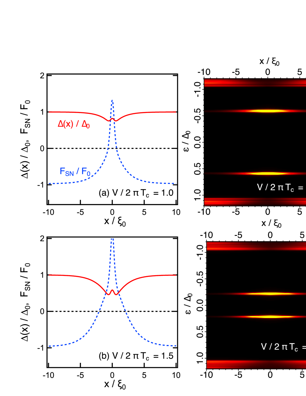
Figure 1: The numerical results of the pair potential $\Delta(x)$ and the free-energy density $F_{\mathrm{SN}}$, and the local density of states $N(x,\epsilon)$ are plotted for several choices of the amplitude of magnetic moment as $|\bm{V}|/2\pi T_{c}=1.0$ in (a), 1.5 in (b), 1.814 in (c), and 2.0 in (d). The pair potential shown with solid line is normalized to $\Delta_{0}$ which is the amplitude of the pair potential in a uniform superconductor at $T=0$. The free-energy density shown with broken is normalized to $F_{0}=N_{0}\Delta_{0}^{2}/2$. The local density of states is shown on the right panel, where we solve the Eilenberger equation for complex energies $\epsilon+i\delta$ with $\delta/2\pi T_{c}=0.005$. The size of a magnetic impurity in Eq. (22) is set as $x_{0}/\xi_{0}=0.5$.

III Sign change in pair potential

In Sec. II, we assume that the pair potential is uniform in real space. In this section, we check the validity of our conclusions in the presence of spatial variation in the pair potential. Especially, we focus on the effects of odd-frequency pairs on the sign change of the pair potential. We solve the Eilenberger equation in a superconductor in one-dimension, where the potential of a magnetic impurity is described by

$$\bm{V}(x)=\bm{V}\,e^{-(\frac{x}{x_{0}})^{2}},$$ (22)

where $x_{0}$ represents the spatial range of the impurity potential. The details of the simulation are shown in Appendix C. We numerically calculate the pair potential in Eq. (109) and the local density of states (LDOS) in Eq. (110). In this section, we measure the length and the energy in units of the coherence length $\xi_{0}=v_{F}/2\pi T_{c}$ and $2\pi T_{c}$, respectively. Here we summarize parameters used in numerical simulation. The length of the superconductor is fixed at 20$\xi_{0}$, $x_{0}$ in Eq. (22) is 0.5 $\xi_{0}$, and the cut-off energy $\omega_{c}$ for the Matsubara frequency is 3 $\times 2\pi T_{c}$.

Figure 1 shows the pair potential and LDOS around a magnetic impurity for several choices of the amplitude of magnetic moment $|\bm{V}|$, where $\Delta_{0}$ is the amplitude of the pair potential in the bulk at $T=0$. The results at $|\bm{V}|/2\pi T_{c}=1.0$ in Fig. 1(a) show the slight suppression of the pair potential around a magnetic impurity. The LDOS on the right panel of (a) indicates the existence of the YSR states around the impurity. The energy of the bound state is about $\epsilon=\pm 0.6\Delta_{0}$ which is relating to the minimum gap size around the impurity. For $|\bm{V}|/2\pi T_{c}=1.5$ in Fig. 1(b), a magnetic impurity suppresses the pair potential further. As a result, the two bound-state energies get closer to the Fermi level as shown in the right panel in (b). The minimum gap size is $0.45\Delta_{0}$ and the energy of a YSR state are $\pm 0.21\Delta_{0}$. Although the minimum gap size for $|\bm{V}|/2\pi T_{c}=1.814$ is $0.26\Delta_{0}$ in Fig. 1(c), the two YSR states exist at almost zero energy. When the magnetic moment increases up to $|\bm{V}|/2\pi T_{c}=2$, the pair potential at the impurity changes the sign and the two bound state energies cross as shown in Fig. 1(d). The one-dimensional superconductor with a magnetic impurity is resemble to SFS junction. The cross of the Andreev bound state energies at an SFS junction is responsible for the transition between the 0-state and the $\pi$-state[46].

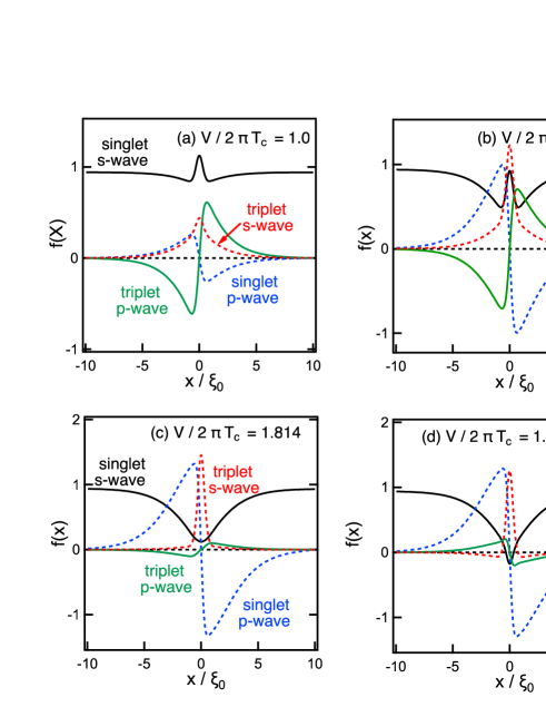
Figure 2: The amplitude of the pairing correlations around the magnetic impurity for (a) $|\bm{V}|/2\pi T_{c}=1$, (b) 1.5, (c) 1.814, and (d) 1.815. The solid (broken) lines are the results of even-frequency (odd-frequency) components. The Matsubara frequency is fixed at $\omega_{n=0}/2\pi T_{c}=0.1$.

In Fig. 2, we plot the amplitude of the pairing correlations around the magnetic impurity at $\omega_{n}/2\pi T_{c}=0.1$, where we choose (a) $|\bm{V}|/2\pi T_{c}=1.0$, (b) 1.5, (c) 1.814, and (d) 1.815. In Fig. 2(a), spin-singlet $s$-wave component is the most dominant and has a small peak at $x=0$, which results in a tiny peak in the pair potential at $x=0$ as shown in Fig. 1(a). The amplitude of even-frequency spin-triplet $p$-wave component is the second most dominant. The odd-frequency spin-triplet $s$-wave and the odd-frequency spin-singlet $p$-wave components shown with broken lines are subdominant everywhere in a superconductor at $|\bm{V}|/2\pi T_{c}=1.0$. The appearance of an odd-frequency pair and the spatial variation in the pair potential are related to each other [47]. In this case, the local odd-frequency pairing correlation generates the tiny peak at $x=0$ in the pair potential in Fig. 1(a). In addition to this, odd-frequency pairs make the superconducting state unstable locally. We calculate the free-energy density in Eq. (112) and plot the results with a broken line in Fig. 1(a). The free-energy density is almost equal to $-F_{0}$ far from the impurity, where $F_{0}=N_{0}\Delta_{0}^{2}/2$ is the condensation energy of the uniform superconducting state measured from the energy of the normal state. The negative free-energy means that the superconducting state is more stable than the normal state. Although the odd-frequency pairing correlations are subdominant as shown in Fig. 2(a), the free-energy density becomes positive at $x=0$ in Fig. 1(a). The positive free-energy at some place does not mean the absence of the pair potential there immediately. Such a locally destroyed superconductivity cannot be a self-consistent solution of the Eilenberger equation. To achieve zero pair potential at the impurity, the spin-singlet $s$-wave correlation must rapidly become zero in real space. This costs the kinetic energy of the superconducting condensate. The nonzero pair potentials under the positive free-energy density are only locally possible in inhomogeneous superconductors. The total free-energy of such an inhomogeneous superconducting state is lower than that in the normal state.

Under spatially uniform pair potential, odd-frequency Cooper pairs are thermodynamically unstable because of their paramagnetic property. The results of the free-energy density in Fig. 1 show that the superconducting state is locally unstable due to the presence of odd-frequency pairs. When we increase the magnetic moment to $|\bm{V}|/2\pi T_{c}=1.5$, the spin-singlet $s$-wave correlation decreases its amplitude slightly as shown in Fig. 2(b). In contrast, the two odd-frequency pairing correlations grow as shown with broken lines. As a result, the free-energy density around $x=0$ in Fig. 1(b) increases and becomes larger than that in (a). In Fig. 2(c), we increase the magnetic moment to $|\bm{V}|/2\pi T_{c}=1.814$. The spin-singlet $s$-wave correlation is suppressed drastically at $x=0$ and the two odd-frequency pairing correlations become dominant locally around the impurity as shown with two broken lines. In Fig. 2(d), we increase the magnetic moment only slightly to $|\bm{V}|/2\pi T_{c}=1.815$. The spin-singlet $s$-wave component changes the sign around $x=0$, which leads to the local sign change of the pair potential. The profiles of the two odd-frequency components, on the other hand, are insensitive to the slight increase of $|\bm{V}|$.

In Fig. 3, we compare the pair potential in (a) and the free-energy density in (b) at the two values of $|\bm{V}|/2\pi T_{c}=1.814$ and 1.815. The abrupt sign change of the pair potential in Fig. 3(a) happens as a result of the finite size effect. The local sign change in the pair potential causes the drastic decrease of the free-energy density as shown in Fig. 3(b). The free-energy for $|x|<0.8\xi_{0}$ in the presence of the sign change is smaller than that in the absence of the sign change. As displayed in both Figs. 2(c) and (d), odd-frequency pairs are dominant in such places. As odd-frequency pairs are paramagnetic, the sign change of the pair potential is one of the possible solutions to decrease the free-energy density. We conclude that odd-frequency pairs generated by a magnetic impurity cause the local $\pi$-phase shift in the pair potential near the impurity.

Finally, we show that the overall sign change in spin-triplet $p$-wave component Figs. 2(c) and (d) do not affect the free-energy density. The pairing correlations are calculated from the parameters $a_{\nu}$ for $\nu=0-3$ as shown in Eqs. (105)-(110). Thus the overall sign change of the pairing correlation is derived from that of $a_{\nu}$, (i.e., $a_{\nu}\to-a_{\nu}$). The induced pairing correlations contribute to the free-energy density through the second term in Eq. (112). The function $\mathcal{N}_{0}$ shown in Eq. (110) consists of the products of $a_{\nu}$ and its particle-hole conjugation $\underline{a}_{\nu}$. Thus the overall sign change of the spin-triplet $p$-wave component does not affect the free-energy density because $a_{\nu}\,\underline{a}_{\nu}$ remains unchanged under $a_{\nu}$ to $-a_{\nu}$.

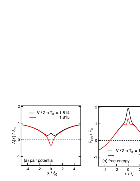
Figure 3: The pair potential (a) and the free-energy density (b) are plotted for $|\bm{V}|/2\pi T_{c}=1.814$ and 1.815. At $|\bm{V}|/2\pi T_{c}=1.815$, the pair potential at $x=0$ changes the sign as shown in (a). As a result of the sign change, the free-energy at $|\bm{V}|/2\pi T_{c}=1.815$ can be smaller than that at $|\bm{V}|/2\pi T_{c}=1.814$.

IV Suppression of $T_{c}$

It has been widely accepted that the transition temperature decreases with the increase of the magnetic impurity concentration since 1960s [10, 11]. We first summarize the outline of these historical papers. The transition temperature is determined by solving the linearized gap equation

$$\Delta=gN_{0}2\pi T\sum_{\omega_{n}>0}F,$$ (23)

where $F$ is the linearized anomalous Green’s function and is $F=F_{0}=\Delta/|\omega_{n}|$ in the clean limit. The anomalous Green’s function is renormalized by the self-energy due to impurity scatterings. For nonmagnetic impurities, the anomalous Green’s function is calculated as

$$F= F_{\mathrm{nm}}=\frac{\tilde{\Delta}}{\tilde{\omega}_{n}},$$ (24)

$$\tilde{\Delta}= \Delta\left[1+\frac{1}{2\tau_{\mathrm{n}}|\omega_{n}|}\right],\;\tilde{\omega}_{n}=\omega_{n}\left[1+\frac{1}{2\tau_{\mathrm{n}}|\omega_{n}|}\right],$$ (25)

where $\tau_{\mathrm{n}}$ is the lifetime of an electron due to scatterings by nonmagnetic impurities. The relation $F_{\mathrm{nm}}=F_{0}$ holds true because the renormalization factor in the numerator of $F_{\mathrm{nm}}$ cancels that in the denominator. As a result, the transition temperature does not change in the presence of nonmagnetic impurities. For magnetic impurities, however, we find within the self-consistent Born approximation that

$$F= F_{\mathrm{m}}=\frac{\tilde{\Delta}}{\tilde{\omega}_{n}}=\frac{\Delta}{|\omega_{n}|+1/\tau_{\mathrm{m}}},$$ (26)

where $\tau_{\mathrm{m}}$ is the lifetime of an electron due to scatterings by magnetic impurities. In Table. 1, we summarize symmetries broken by the self-energy due to magnetic impurities. Thus translational symmetry, local inversion symmetry, and spin-rotation symmetry are restored after averaging. The renormalization factor of $\omega_{n}$ and that of $\Delta$ can be different from each other because the magnetic moments of impurities break time-reversal symmetry

$$\hat{\sigma}_{2}\,\bm{V}\cdot\hat{\bm{\sigma}}^{\ast}\,\hat{\sigma}_{2}=-\bm{V}\cdot\hat{\bm{\sigma}}.$$ (27)

The negative sign on the right-hand side is the source of $1/\tau_{\mathrm{m}}$ in Eq. (26) that explains the suppression of $T_{c}$. Indeed, the transition temperature is estimated as

$$\log\left(\frac{T_{c}}{T_{0}}\right)\approx\psi\left(\frac{1}{2}\right)-\psi\left(\frac{1}{2}+\frac{\xi_{0}}{\ell_{m}}\frac{T_{0}}{T_{c}}\right),$$ (28)

$$\psi\left(\frac{1}{2}\right)-\psi\left(\frac{1}{2}+\frac{x}{2}\right)$$

$$=\sum_{n=0}^{\infty}\frac{2}{2n+1+x}-\sum_{n=0}^{\infty}\frac{2}{2n+1},$$ (29)

where $T_{0}$ is the transition temperature in the clean limit, $\ell_{\mathrm{m}}=v_{F}\,\tau_{\mathrm{m}}$ is the mean free path of an electron due to scatterings by magnetic impurities, and $\psi(x)$ is the digamma function. As shown with a broken line in Fig. 4, $T_{c}$ decreases rapidly with the increase of $\xi_{0}/\ell_{\mathrm{m}}$. We note that neither spin-triplet pairing correlations nor odd-frequency pairing correlations are considered on the way to Eq. (28).

Secondly, we discuss how odd-frequency pairs affect the transition temperature. To do this, we derive the linearized Eilenberger equation which are displayed in Eqs. (113) and (114). The gap equation in the linearized regime is given in Eq. (115). We consider a pair of the classical trajectories: one is along $\hat{\bm{k}}$ and the other along $-\hat{\bm{k}}$. As a result, we obtain following equations which relates the four pairing correlations belonging to different symmetry classes,

$$v_{F}\hat{\bm{k}}\cdot\nabla S_{-}+2\omega_{n}\,S_{+}-2i\bm{T}_{+}\cdot\bm{V}$$

$$-2\mathrm{sgn}(\omega_{n})\,\Delta=0,$$ (30)

$$v_{F}\hat{\bm{k}}\cdot\nabla\bm{T}_{-}+2\omega_{n}\,\bm{T}_{+}-2iS_{+}\bm{V}=0,$$ (31)

$$v_{F}\hat{\bm{k}}\cdot\nabla S_{+}+2\omega_{n}\,S_{-}-2i\bm{T}_{-}\cdot\bm{V}=0,$$ (32)

$$v_{F}\hat{\bm{k}}\cdot\nabla\bm{T}_{+}+2\omega_{n}\,\bm{T}_{-}-2iS_{-}\bm{V}=0,$$ (33)

$$S_{\pm}(\bm{r},\hat{\bm{k}},\omega_{n})=a_{0}(\bm{r},\hat{\bm{k}},\omega_{n})\pm a_{0}(\bm{r},-\hat{\bm{k}},\omega_{n}),$$ (34)

$$\bm{T}_{\pm}(\bm{r},\hat{\bm{k}},\omega_{n})=\bm{a}(\bm{r},\hat{\bm{k}},\omega_{n})\pm\bm{a}(\bm{r},-\hat{\bm{k}},\omega_{n}).$$ (35)

The Riccati’s parameter $S_{+}(S_{-})$ represents the spin-singlet even-parity (odd-parity) pairing correlation and $\bm{T}_{+}(\bm{T}_{-})$ represents the spin-triplet even-parity (odd-parity) pairing correlation. Equation (30) describes the relation among the three spin-singlet even-parity pairing correlations and the pair potential. The spatial gradient of the odd-parity correlation $S_{-}$ generates the even-parity component, which is a result of breaking local inversion symmetry. For simplicity, we neglect the effects of breaking local inversion symmetry and delete the gradient terms in real space in Eqs. (30)-(33). In this approximation, we implicitly consider the homogeneous correlation functions after averaging over the position of magnetic impurities. The correlation functions under the approximation recover both translational symmetry and local inversion symmetry.

In the absence of gradient terms in real space, $S_{-}=\bm{T}_{-}=0$ is a solution of Eqs. (32) and (33). The odd-frequency correlation $\bm{T}_{+}$ contributes to the spin-singlet pairing correlation as a result of breaking spin-rotation symmetry by magnetic impurities. In what follows, we analyze the two remaining equations in Eqs. (30) and (31) in the absence of gradient terms. Eq. (31) implies that the magnetic moment generates the odd-frequency spin-triplet pairing correlation $\bm{T}_{+}$ from the spin-singlet even-parity correlation $S_{+}$ in the absence of spin-rotation symmetry. The Matsubara frequency $\omega_{n}$ at the second term enables the conversion from the odd-frequency correlation $\bm{T}_{+}$ to the even-frequency correlation $S_{+}$. As a result of the conversion, the free-energy density at a magnetic impurity increases above zero as shown in Fig. 1. The free-energy averaged over a whole superconductor increases and the transition temperature decreases with the increase of the magnetic impurity concentration. The superconducting state disappears when the averaged free-energy becomes zero. By eliminating the odd-frequency pairing correlation $\bm{T}_{+}$ at Eqs. (30) and (31), we reach an equation only for the spin-singlet even-parity component,

$$\omega_{n}^{2}S_{+}+\bm{V}\cdot\bm{V}S_{+}=\Delta|\omega_{n}|.$$ (36)

We assume the properties of random potential

$$\overline{\bm{V}(\bm{r})}=0,\quad\overline{\bm{V}(\bm{r})\bm{V}(\bm{r})}=\frac{1}{\tau_{s}^{2}}$$ (37)

under ensemble averaging, where $1/\tau_{s}$ can be interpreted as the lifetime of a spin-singlet Cooper pair in the presence of magnetic impurities. This can be confirmed by changing $i\omega_{n}\to-\partial_{\tau}\to-i\partial_{t}$ in Eq. (36). We find that $\tau_{s}$ gives the characteristic time scale of the equation. We finally reach a solution of

$$S_{+}= \frac{\Delta\,|\omega_{n}|}{\omega_{n}^{2}+1/\tau_{s}^{2}}.$$ (38)

The scatterings by magnetic impurities remove the singularity at $\omega_{n}=0$ at the denominator. This explains the decrease of $T_{c}$ when we substitute $F=S_{+}$ into Eq. (23). In Fig. 4, we show $T_{c}$ calculated by using Eq. (38) with a solid line, where the horizontal axis is $\xi_{0}/\ell_{s}$ with $\ell_{s}=\tau_{s}v_{F}$ meaning the mean-free path of a spin-singlet $s$-wave Cooper pair under magnetic impurities. The calculated results show that $T_{c}$ decreases with the increase of scatterings by magnetic impurities. This phenomenon can be understood from two different viewpoints because magnetic impurities simultaneously generate odd-frequency Cooper pairs and subgap quasiparticles. The viewpoint from a Cooper pair shows that the odd-frequency pair increases the free-energy locally. The viewpoint from a quasiparticle suggests that the occupation of the YSR states below the Fermi level reduces the condensation energy. We conclude that these two facts make the superconducting state unstable and decrease $T_{c}$.

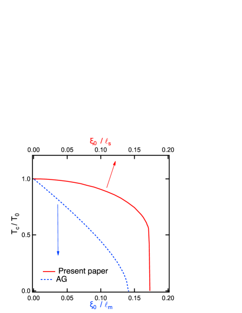
Figure 4: The theoretical results of transition temperature are plotted as a function of the inverse of the mean-free path. The broken line is the results calculated from the impurity self-energy within the self-consistent Born approximation, where we use Eq. (26). The solid line is the results of this paper, where we use Eq. (38). It is impossible to compare $T_{c}$ in the two results because the horizontal lines are defined in different ways. In Eq. (26), $\ell_{\mathrm{m}}=v_{F}\tau_{\mathrm{m}}$ is the mean-free path of an electron on the Fermi level. In Eq. (38), on the other hand, $\ell_{s}=\tau_{s}v_{F}$ can be interpreted as the mean-free path of a spin-singlet Cooper pair.

V Conclusion

We have studied the properties of superconducting state around a magnetic impurity embedded in a conventional superconductor. The analytical results of the anomalous Green’s function show that the magnetic impurity converts a spin-singlet $s$-wave Cooper pair into odd-frequency Cooper pairs. Comparing the normal and the anomalous Green’s function explains the coexistence of odd-frequency Cooper pairs and quasiparticles at the Yu-Shiba-Rusinov (YSR) states. We conclude that the formation of the YSR states below the gap is a direct consequence of the appearance of an odd-frequency Cooper pair.

The numerical results of the free-energy density show that the superconducting states around a magnetic impurity are thermodynamically unstable because of the paramagnetic property of odd-frequency Cooper pairs. This fact explains naturally the remaining open issues listed in the introduction. The sign of the pair potential changes around an impurity with sufficiently large magnetic moment because odd-frequency pairs are dominant around such a strong magnetic impurity. On the basis of obtained results, we also proposed an alternative scenario to explain the suppression of the transition temperature in the presence of many magnetic impurities.

Appendix A Paramagnetic Cooper pairs

The superconducting condensate can be described phenomenologically by the macroscopic wave function

$$\psi(\bm{r})=\sqrt{n_{\mathrm{S}}(\bm{r})}\,e^{i\theta(\bm{r})},$$ (39)

where $n_{\mathrm{S}}$ is the density of Cooper pairs and $\theta$ is the phase of the condensate. The flux quantization is derived from the singlevaluedness of this wave function. The Josephson effect is explained as the tunnel effect between two superconductors characterized by such wave functions. The energy of the condensate can be calculated in terms of the macroscopic wave function

$$E= \int d\bm{r}\,\frac{\hbar^{2}}{2m}\left\{\left(\nabla+i\frac{e}{\hbar c}\bm{A}\right)\psi^{\dagger}(\bm{r})\right\}\left\{\left(\nabla-i\frac{e}{\hbar c}\bm{A}\right)\psi(\bm{r})\right\},$$ (40)

$$= \int d\bm{r}\,\frac{\hbar^{2}}{2m}\left\{\frac{(\nabla n_{\mathrm{S}})^{2}}{4n_{\mathrm{S}}}+n_{\mathrm{S}}\left(\nabla\theta-\frac{e}{\hbar c}\bm{A}\right)^{2}\right\}.$$ (41)

The first term in Eq.  (41) represents the kinetic energy of the condensate and the second term means the elastic energy of the superconducting phase. Since $n_{\mathrm{S}}>0$, both the spatial gradient of the density and the spatial gradient of the phase increase the energy of the condensate, which describes the rigidity of the superconducting state. Therefore, both the pair density and the phase are uniform at the ground state in the absence of a magnetic field. The electric current can be described by

$$\bm{j}= \frac{e\,\hbar}{2im}\left[\psi^{\dagger}(\bm{r})\left(\nabla-i\frac{e}{\hbar c}\bm{A}\right)\psi(\bm{r})-\left(\nabla+i\frac{e}{\hbar c}\bm{A}\right)\psi^{\dagger}(\bm{r})\;\psi(\bm{r})\right]=\frac{e\,\hbar\,n_{\mathrm{S}}}{m}\nabla\theta-\frac{n_{\mathrm{S}}\,e^{2}}{mc}\bm{A}.$$ (42)

Together with the Maxwell equation $\nabla\times\bm{H}=\frac{4\pi}{c}\bm{j}$, we obtain the equation for a magnetic field in a superconductor

$$\nabla^{2}\bm{H}-\frac{4\pi\,n_{\mathrm{S}}e^{2}}{m\,c^{2}}\,\bm{H}=0.$$ (43)

The London’s length $\lambda_{\mathrm{L}}=\sqrt{m\,c^{2}/4\pi\,n_{\mathrm{S}}\,e^{2}}$ characterizes the spatial variation of a magnetic field. Equation (43) represents the Meissner screening effect of a magnetic field. The dumping of a magnetic field into a superconductor is described by the negative sign at the second term on the last line in Eq. (42). The argument above is valid when the pair density $n_{\mathrm{S}}$ is positive everywhere in a superconductor.

Let us assume that the pair density is negative locally at a finite area around $\bm{r}=\bm{r}_{0}$ and discuss the physical consequence of $n_{\mathrm{S}}(\bm{r}_{0})<0$. The second term in Eq. (41) suggests that large gradient of the phase and the penetration of magnetic field is necessary to decrease the energy of the condensate. Namely the condensate with the ”negative pair density” is paramagnetic. Equation (43) with negative $n_{\mathrm{S}}$ suggests also that a magnetic field can penetrate into such a paramagnetic superconductor [40, 41]. Such local area around $\bm{r}_{0}$ may be no longer superconductive because the phase $\theta$ fluctuates easily from a constant value. Thus the pair density $n_{\mathrm{S}}$ must be positive to realize the stable homogeneous superconducting ground state both electromagnetically and thermodynamically. However, ”pair density” can be negative locally in the presence of an odd-frequency pair.

A surface of a superconductor breaks inversion symmetry locally. As a result of breaking inversion symmetry, odd-parity (even-parity) pairing correlations appear at a surface of even-parity (odd-parity) superconductor. Such induced pairing correlations belong to odd-frequency symmetry class because the surface does not change spin of a Cooper pair. In what follows, we demonstrate that the pair density can be negative at such a surface by using an analytical solution of the Eilenberger equation,

$$\hbar v_{F}{\hat{\bm{k}}}\cdot\nabla\hat{g}+[H,\hat{g}]=0,$$ (44)

$$H=\left[\begin{array}[]{cc}\omega_{n}&\Delta(\bm{r},\hat{\bm{k}})\\ -s_{s}\undertilde{\Delta}(\bm{r},\hat{\bm{k}})&-\omega_{n}\end{array}\right],\quad\hat{g}(\bm{r},\hat{\bm{k}},\omega_{n})=\left[\begin{array}[]{cc}g(\bm{r},\hat{\bm{k}},\omega_{n})&f(\bm{r},\hat{\bm{k}},\omega_{n})\\ -s_{s}\undertilde{f}(\bm{r},\hat{\bm{k}},\omega_{n})&-g(\bm{r},\hat{\bm{k}},\omega_{n})\end{array}\right].$$ (49)

Here we have reduced to $2\times 2$ particle-hole space by extracting one spin sector of the Bogoliubov-de Gennes (BdG) Hamiltonian. The pair potential obeys the symmetry relation

$$\Delta(\bm{r},-\hat{\bm{k}})=\left\{\begin{array}[]{rl}\Delta(\bm{r},\hat{\bm{k}})&\text{singlet}\;s_{s}=-1\\ -\Delta(\bm{r},\hat{\bm{k}})&\text{triplet}\;s_{s}=1,\end{array}\right.$$ (52)

which is drived from the Fermi-Dirac statistics of electrons. The Eilenberger equation can be decomposed into three equations [47],

$$v_{F}\hat{\bm{k}}\cdot\nabla g= 2\Delta\,f_{S},\quad v_{F}\hat{\bm{k}}\cdot\nabla f_{B}=-2\omega_{n}\,f_{S},\quad v_{F}\hat{\bm{k}}\cdot\nabla f_{S}=2(\Delta\,g-\omega_{n}\,f_{B}),$$ (53)

with

$$f_{B}= \frac{1}{2}(f-s_{s}\undertilde{f}),\quad f_{S}=\frac{1}{2}(f+s_{s}\undertilde{f}).$$ (54)

The quasiclassical Green’s functions satisfy the normalization condition

$$g^{2}-s_{s}\undertilde{f}\,f=g^{2}+f_{B}^{2}-f_{S}^{2}=1.$$ (55)

In a homogeneous superconductor, we obtain the solution as

$$g=\frac{\omega_{n}}{\Omega},\quad f_{B}=\frac{\Delta(\hat{\bm{k}})}{\Omega},\quad f_{S}=0,\quad\Omega=\sqrt{\omega_{n}^{2}+\Delta^{2}(\hat{\bm{k}})}.$$ (56)

Thus $f_{B}$ is interpreted as bulk component of pairing correlation which contributes to the pair potential through the gap equation

$$\Delta(\bm{r},\hat{\bm{k}})=T\sum_{\omega_{n}}\,\int\frac{d\hat{\bm{k}}^{\prime}}{S_{d}}\lambda(\hat{\bm{k}},\hat{\bm{k}}^{\prime})f(\bm{r},\hat{\bm{k}}^{\prime},\omega_{n}),$$ (57)

where $\lambda$ represents an attractive interaction between two electrons. The second equation in Eq. (53) represents the symmetry relationship between $f_{B}$ and $f_{S}$. Since $\hat{\bm{k}}$ is an odd-parity function and $\omega_{n}$ is an odd in Matsubara frequency, $f_{S}$ belongs to the opposite parity and opposite frequency symmetry class to $f_{B}$. Therefore $f_{S}$ is considered as an induced pairing component due to the spatial gradient of $f_{B}$. Although the anomalous Green’s function $f$ in Eq. (57) consists of both $f_{B}$ and $f_{S}$, only the bulk component $f_{B}$ contributes to the pair potential. Since $f_{S}$ is an odd-function of $\omega_{n}$, the summation of $f_{S}$ over $\omega_{n}$ vanishes. The Meissner kernel for the quasiclassical Green’s function is described as [48]

$${j}_{\mu}= -\frac{2ne^{2}}{mc}\mathcal{Q}_{\mu,\nu}{A}_{\nu},$$ (58)

$$\mathcal{Q}_{\mu,\nu}= d\pi T\sum_{\omega_{n}}\int\frac{d\hat{\bm{k}}}{S_{d}}\hat{k}_{\mu}\,\hat{k}_{\nu}\,\partial_{\omega_{n}}g(\bm{r},\hat{\bm{k}},\omega_{n})=d\pi T\sum_{\omega_{n}>0}\int\frac{d\hat{\bm{k}}}{S_{d}}\hat{k}_{\mu}\,\hat{k}_{\nu}\,(f_{B}^{2}-f_{S}^{2})\,\partial_{\omega_{n}}\log\frac{1+g}{1-g}.$$ (59)

The last expression suggests that the odd-frequency pairing correlation decreases $\mathcal{Q}_{\mu,\nu}$. By putting the results in Eq. (56) for a spin-singlet $s$-wave superconductor into $\mathcal{Q}$, it is possible to recover the results of [49]

$$\mathcal{Q}_{\mu,\nu}=\pi\,T\sum_{\omega_{n}}\frac{\Delta^{2}}{(\omega_{n}^{2}+\Delta^{2})^{3/2}}\delta_{\mu,\nu}.$$ (60)

The product of $n\,\mathcal{Q}_{\mu,\mu}$ is often referred to as pair density.

As an example of inhomogeneous superconducting states, we consider the condensate near the surface of a two-dimensional $p$-wave superconductor. The pair potential is described as

$$\Delta(x)=\Delta\cos\theta\tanh\left(\frac{x}{\xi_{0}}\right),\quad\hat{k}_{x}=\cos\theta,\quad\hat{k}_{y}=\sin\theta,\quad\xi_{0}=\frac{v_{F}}{\Delta\cos\theta},$$ (61)

where we assume that a surface is at $x=0$ and a $p$-wave superconductor occupies $x>0$, the superconducting state is uniform in the $y$ direction, and $\xi_{0}$ is the coherence length. The solution of Eq. (53) can be obtained as [50]

$$g(x,\theta,\omega_{n})= \frac{\omega_{n}}{\Omega_{\theta}}+\frac{\Delta^{2}\cos^{2}\theta}{2\omega_{n}\Omega_{\theta}}\cosh^{-2}\left(\frac{x}{\xi_{0}}\right),\quad f_{B}(x,\theta,\omega_{n})=\frac{\Delta\cos\theta}{\Omega_{\theta}}\tanh\left(\frac{x}{\xi_{0}}\right),$$ (62)

$$f_{S}(x,\theta,\omega_{n})= -\frac{\Delta^{2}\cos^{2}\theta}{2\omega_{n}\Omega_{\theta}}\cosh^{-2}\left(\frac{x}{\xi_{0}}\right),\quad\Omega_{\theta}=\sqrt{\omega_{n}^{2}+\Delta^{2}\cos^{2}\theta}.$$ (63)

The bulk component $f_{B}(x,\theta+\pi,\omega_{n})=-f_{B}(x,\theta,\omega_{n})$ is odd-parity, whereas the surface component $f_{S}$ is even-parity because of $\cos^{2}(\theta+\pi)=\cos^{2}\theta$. The gap equation in Eq. (57) is described as

$$\Delta(x)= T\sum_{\omega_{n}}\,\int_{0}^{2\pi}\frac{d\theta^{\prime}}{2\pi}(2\lambda\,\cos\theta\,\cos\theta^{\prime})\left[f_{B}(x,\theta^{\prime},\omega_{n})+f_{S}(x,\theta^{\prime},\omega_{n})\right],$$ (64)

$$= \Delta\,\cos\theta\,\tanh\left(\frac{x}{\xi_{0}}\right)\lambda T\sum_{\omega_{n}}\frac{1}{\sqrt{\omega_{n}^{2}+\Delta^{2}}}.$$ (65)

On the way to the second line, we approximately neglect $\theta$ dependence of $\Omega_{\theta}$ and that of $\xi_{0}$ in $f_{\mathrm{B}}$. The amplitude of $f_{S}$ increases with the decrease of $\omega_{n}$ at its denominator and can be larger than the amplitude of $f_{B}$ for $\omega_{n}\ll\Delta$. The resulting response kernel

$$\mathcal{Q}_{\mu,\nu}\approx\delta_{\mu,\nu}\,\pi T\sum_{\omega_{n}}\,\int_{0}^{2\pi}\frac{d\theta}{2\pi}\frac{\Delta^{2}\cos^{2}\theta}{(\omega_{n}^{2}+\Delta^{2}\cos^{2}\theta)^{3/2}}\left[1-\frac{\Delta^{2}\cos^{2}\theta}{2\omega_{n}^{2}}\cosh^{-2}\left(\frac{x}{\xi_{0}}\right)\right],$$ (66)

can be negative for a low temperature $T\ll T_{c}$ near the surface $0<x<\xi_{0}$. The paramagnetic response at a surface of unconventional superconductor was pointed out for a $d$-wave superconductor [51, 52]. To make clear the details of paramagnetic effect theoretically, analysis beyond the linear response is necessary. In Refs. [42, 53], the pair potential and a magnetic filed are determined self-consistently with each other in a small unconventional superconductor. A small $p$-wave superconducting disk shows paramagnetic response to a magnetic filed at a low temperature. Even-frequency pairs stabilize $p$-wave superconductivity in the bulk and odd-frequency pairs exhibit the paramagnetic response at the surface.

Finally, we briefly explain the coexistence of an odd-frequency pair and a quasiparticle at the Andreev bound state at a surface. After applying $i\omega_{n}\to\epsilon+i\delta$, the local density of states for $|\epsilon|<\Delta$ calculated from the second term of the normal Green’s function becomes

$$\frac{N(x,\epsilon)}{N_{0}}=\mathrm{Re}\int\frac{d\theta}{2\pi}i\frac{\Delta^{2}\cos^{2}\theta}{2(\epsilon+i\delta)\sqrt{\Delta^{2}\cos^{2}\theta-\epsilon^{2}}}\cosh^{-2}\left(\frac{x}{\xi_{0}}\right)\to\delta(\epsilon)\,\frac{\Delta}{\pi}\cosh^{-2}\left(\frac{x}{\xi_{0}}\right).$$ (67)

The peak of the local density of states at zero energy reflects the existence of a quasiparticle at the surface Andreev bound state.

Appendix B Lippmann-Schwinger equation

The Lippmann-Schwinger equation relates the Green’s function in the presence of perturbations $\check{V}$ to the Green’s function in the absence of perturbation as

$$\check{\mathcal{G}}(\bm{r},\bm{r}^{\prime})=\check{\mathcal{G}}^{(0)}(\bm{r},\bm{r}^{\prime})+\int d\bm{r}_{1}\;\check{\mathcal{G}}^{(0)}(\bm{r},\bm{r}_{1})\,\check{V}(\bm{r}_{1})\,\check{\mathcal{G}}^{(}\bm{r}_{1},\bm{r}^{\prime}).$$ (68)

When we consider an impurity potential $\check{V}(\bm{r})=\check{V}\delta(\bm{r})$, the equation becomes

$$\check{\mathcal{G}}(\bm{r},\bm{r}^{\prime})=\check{\mathcal{G}}^{(0)}(\bm{r},\bm{r}^{\prime})+\check{\mathcal{G}}^{(0)}(\bm{r},0)\,\check{V}\,\check{\mathcal{G}}(0,\bm{r}^{\prime}).$$ (69)

By putting $\bm{r}=0$ into the equation, the equation

$$\check{\mathcal{G}}(0,\bm{r}^{\prime})=\check{\mathcal{G}}^{(0)}(0,\bm{r}^{\prime})+\check{\mathcal{G}}^{(0)}(0,0)\,\check{V}\,\check{\mathcal{G}}(0,\bm{r}^{\prime})$$ (70)

has a closed form. Substituting the solution

$$\check{\mathcal{G}}(0,\bm{r}^{\prime})=\left[1-\check{\mathcal{G}}^{(0)}(0,0)\check{V}\right]^{-1}\check{\mathcal{G}}^{(0)}(0,\bm{r}^{\prime})$$ (71)

into Eq. (69), we obtain

$$\check{\mathcal{G}}(\bm{r},\bm{r}^{\prime})=\check{\mathcal{G}}^{(0)}(\bm{r},\bm{r}^{\prime})+\check{\mathcal{G}}^{(0)}(\bm{r},0)\,\check{V}\,\left[1-\check{\mathcal{G}}^{(0)}(0,0)\check{V}\right]^{-1}\check{\mathcal{G}}^{(0)}(0,\bm{r}^{\prime}).$$ (72)

In this paper, we consider a spin-singlet $s$-wave superconductor in one-dimension as described by Eq. (3). The unperturbed Green’s function in the Matsubara representation is given by

$$\check{\mathcal{G}}^{(0)}(x,x^{\prime})= -\frac{\pi N_{0}}{\Omega}\check{U}^{\dagger}\left[\begin{array}[]{cc}i\omega_{n}C_{0}-\Omega S_{0}&\Delta C_{0}\\ \Delta C_{0}&i\omega_{n}C_{0}+\Omega S_{0}\end{array}\right]e^{-|x-x^{\prime}|/\xi_{0}}\check{U},$$ (75)

with

$$\Omega= \sqrt{\omega_{n}^{2}+\Delta^{2}},\quad k_{\pm}=k\left(1\pm i\frac{\Omega}{2\epsilon_{F}}\right),\quad\check{U}=\left[\begin{array}[]{cc}1&0\\ 0&i\hat{\sigma}_{2}e^{i\varphi}\end{array}\right],$$ (78)

$$C_{0}= \cos(k|x-x^{\prime}|),\quad S_{0}=\sin(k|x-x^{\prime}|),\quad\xi_{0}=\frac{2\epsilon_{F}}{\Omega k_{F}},$$ (79)

where $\hat{\sigma}_{j}$ for $j=1-3$ is the Pauli’s matrix in spin space and $k$ denotes the Fermi wavenumber.

The potential of a nonmagnetic impurity is described by

$$\check{V}=\left[\begin{array}[]{cc}V_{0}\hat{\sigma}_{0}&0\\ 0&-V_{0}\hat{\sigma}_{0}\end{array}\right]=V_{0}\hat{\tau}_{3},$$ (82)

where $\hat{\tau}_{j}$ for $j=1-3$ is the Pauli’s matrix in particle-hole space. The Green’s function in the presence of a nonmagnetic impurity is calculates as

$$\check{\mathcal{G}} (x,x^{\prime})=\check{\mathcal{G}}^{(0)}(x,x^{\prime})-\frac{\pi N_{0}}{\Omega}e^{-(|x|+|x^{\prime}|)/\xi_{0}}\frac{\gamma_{0}}{(1+\gamma_{0}^{2})}$$

$$\times\check{U}^{\dagger}\left[\begin{array}[]{cc}i\omega(S_{+}-\gamma_{0}C_{+})+\Omega(C_{+}+\gamma_{0}S_{+})&\Delta(S_{+}-\gamma_{0}C_{+})\\ \Delta(S_{+}-\gamma_{0}C_{+})&i\omega(S_{+}-\gamma_{0}C_{+})-\Omega(C_{+}+\gamma_{0}S_{+})\end{array}\right]\check{U},$$ (85)

$$C_{\pm}=\cos\left\{k(|x|\pm|x^{\prime}|)\right\},\quad S_{\pm}=\sin\left\{k(|x|\pm|x^{\prime}|)\right\},\quad\gamma_{0}=\pi N_{0}V_{0}.$$ (86)

The anomalous Green’s function results in

$$\hat{f}(x,x^{\prime})=-\frac{\pi N_{0}\Delta}{\Omega}\,i\hat{\sigma}_{2}\,\left[C_{0}\,e^{-|x-x^{\prime}|/\xi_{0}}+\frac{\gamma_{0}}{1+\gamma_{0}^{2}}\left(S_{+}-\gamma_{0}\,C_{+}\right)e^{-(|x|+|x^{\prime}|)/\xi_{0}}\right].$$ (87)

The anomalous Green’s function $\hat{f}(x,x^{\prime})$ consists only of a spin-singlet even-parity Cooper pair because it remains unchanged under $x\leftrightarrow x^{\prime}$. The normal Green’s function becomes

$$\mathrm{Tr}\left[\check{\mathcal{G}}^{R}_{\epsilon}(x,x)\right]=\frac{-4\pi i\,N_{0}\,\epsilon}{\sqrt{\epsilon^{2}-\Delta^{2}}}\left[1+\frac{\gamma_{0}}{1+\gamma_{0}^{2}}\left(\sin 2k|x|-\gamma_{0}\,\cos 2k|x|\right)e^{-2|x|/\xi_{0}}\right],$$ (88)

which is always real value for $\epsilon<\Delta$.

In the presence of a magnetic impurity, the normal Green’s function is calculated to be

$$\hat{g}(x,x^{\prime})= \frac{\pi N_{0}}{\Omega}\left[-e^{-|x-x^{\prime}|/\xi_{0}}(i\omega_{n}C_{0}-\Omega S_{0})\right.$$

$$-\frac{e^{-(|x|+|x^{\prime}|)/\xi_{0}}}{Z}|\bm{\gamma}|^{2}\left[2i\omega_{n}\Delta^{2}C_{-}+\left\{\Delta^{2}(1-|\bm{\gamma}|^{2})-\omega_{n}^{2}(1+|\bm{\gamma}|^{2})\right\}(i\omega_{n}C_{+}-\Omega S_{+})\right]$$

$$+\frac{e^{-(|x|+|x^{\prime}|)/\xi_{0}}}{Z}\bm{\gamma}\cdot\hat{\bm{\sigma}}\Omega\left.\left[\Delta^{2}(1-|\bm{\gamma}|^{2})C_{-}+i\omega_{n}(i\omega_{n}C_{+}-\Omega S_{+})(1+|\bm{\gamma}|^{2})\right]\right],$$ (89)

$$Z= \Delta^{2}(1-|\bm{\gamma}|^{2})^{2}+\omega_{n}^{2}(1+|\bm{\gamma}|^{2})^{2},\quad\bm{\gamma}=\pi N_{0}\bm{V}.$$ (90)

where $S_{\pm}$ and $C_{\pm}$ are given in Eq. (86) The anomalous Green’s function is displayed in Eq. (15).

Appendix C Eilenberger equation

To study the pairing correlations around a magnetic impurity, we solve the Eilenberger equation numerically. The Matsubara Green function can be decomposed into the Riccati parameters as,

$$\check{\mathcal{G}}(\bm{r},\hat{\bm{k}},i\omega_{n})= \left(\begin{array}[]{cc}\hat{\mathcal{G}}&\hat{\mathcal{F}}\\ \underline{\hat{\mathcal{F}}}&-\underline{\hat{\mathcal{G}}}\end{array}\right)=\left(\begin{array}[]{cc}{\hat{\mathcal{N}}}&{\hat{0}}\\ {\hat{0}}&\underline{\hat{\mathcal{N}}}\end{array}\right)\left(\begin{array}[]{cc}\mathrm{sgn}(\omega_{n})\,(1-\hat{a}\underline{\hat{a}})&2\hat{a}\\ 2\underline{\hat{a}}&-\mathrm{sgn}(\omega_{n})\,(1-\underline{\hat{a}}\hat{a})\end{array}\right),$$ (97)

$$\hat{a}=\hat{a}(\bm{r},\hat{\bm{k}},i\omega_{n}),\qquad\underline{\hat{a}}=\underline{\hat{a}}(\bm{r},\hat{\bm{k}},i\omega_{n}),$$ (98)

$$\hat{\mathcal{N}}=(1+\hat{a}\underline{\hat{a}})^{-1},\qquad\underline{\hat{\mathcal{N}}}=(1+\underline{\hat{a}}\hat{a})^{-1}.$$ (99)

The Riccati parameters can be decomposed into four components as

$$\hat{a}(\bm{r},\hat{\bm{k}},i\omega_{n})= a_{0}(\bm{r},\hat{\bm{k}},i\omega_{n})+\bm{a}(\bm{r},\hat{\bm{k}},i\omega_{n})\cdot\hat{\bm{\sigma}},$$ (100)

where $a_{0}$ is the spin-singlet component and $a_{j}$ for $j=1-3$ are three spin-triplet components. They obey the symmetry relations

$$a_{0}(\bm{r},-\hat{\bm{k}},-i\omega_{n})=a_{0}(\bm{r},\hat{\bm{k}},i\omega_{n}),\quad\bm{a}(\bm{r},-\hat{\bm{k}},-i\omega_{n})=-\bm{a}(\bm{r},\hat{\bm{k}},i\omega_{n}).$$ (101)

The spin-singlet component $a_{0}$ is either the even-parity even-frequency symmetry or odd-party odd-frequency one. The three spin-triplet component $\bm{a}$ are either the odd-parity even-frequency symmetry or even-party odd-frequency one. The Riccati parameter $\hat{a}$ in Eq. (98) obeys the Eilenberger equation,

$$i\hbar v_{F} \hat{\bm{k}}\cdot\nabla\hat{a}+2i\omega_{n}\,\hat{a}+\bm{V}(\bm{r})\cdot\bm{\sigma}\,\hat{a}+\hat{a}\,\bm{V}(\bm{r})\cdot\bm{\sigma}-i\;\mathrm{sgn}(\omega_{n})\,\Delta(\bm{r})+i\;\mathrm{sgn}(\omega_{n})\,\hat{a}\,\underline{\Delta}(\bm{r})\,\hat{a}=0,$$ (102)

$$i\hbar v_{F} \hat{\bm{k}}\cdot\nabla\hat{\underline{a}}-2i\omega_{n}\,\hat{\underline{a}}-\bm{V}(\bm{r})\cdot\bm{\sigma}\,\hat{\underline{a}}-\hat{\underline{a}}\,\bm{V}(\bm{r})\cdot\bm{\sigma}+i\;\mathrm{sgn}(\omega_{n})\,\underline{\Delta}(\bm{r})-i\;\mathrm{sgn}(\omega_{n})\,\hat{\underline{a}}\,\Delta(\bm{r})\,\hat{\underline{a}}=0.$$ (103)

The equation

$$\underline{X}(\bm{r},\hat{\bm{k}},i\omega_{n})=\hat{\sigma}_{2}\,\undertilde{X}(\bm{r},\hat{\bm{k}},i\omega_{n})\,\hat{\sigma}_{2}=\hat{\sigma}_{2}\,X^{\ast}(\bm{r},-\hat{\bm{k}},i\omega_{n})\,\hat{\sigma}_{2},$$ (104)

defines the relation among $X$, $\undertilde{X}$, and $\underline{X}$.

The anomalous Green’s function is represented by

$$\hat{\mathcal{F}}(\bm{r},\hat{\bm{k}},i\omega_{n})= 2\,\hat{\mathcal{N}}(\bm{r},\hat{\bm{k}},i\omega_{n})\,\hat{a}(\bm{r},\hat{\bm{k}},i\omega_{n})=\mathcal{F}_{0}(\bm{r},\hat{\bm{k}},i\omega_{n})+\bm{\mathcal{F}}(\bm{r},\hat{\bm{k}},i\omega_{n})\cdot\hat{\bm{\sigma}},$$ (105)

$$\mathcal{F}_{0}(\bm{r},\hat{\bm{k}},i\omega_{n})= \frac{2}{Z_{N}}\left[a_{0}+(a_{0}^{2}-\bm{a}^{2})\,\underline{a}_{0}\right]_{(\bm{r},\hat{\bm{k}},i\omega_{n})},$$ (106)

$$\bm{\mathcal{F}}(\bm{r},\hat{\bm{k}},i\omega_{n})= \frac{2}{Z_{N}}\left[\bm{a}+(a_{0}^{2}-\bm{a}^{2})\,\underline{\bm{a}}\right]_{(\bm{r},\hat{\bm{k}},i\omega_{n})},$$ (107)

$$Z_{N}= 1+(a_{0}^{2}-\bm{a}\cdot\bm{a})(\underline{a}_{0}^{2}-\underline{\bm{a}}\cdot\underline{\bm{a}})+2(a_{0}\,\underline{a}_{0}-\bm{a}\cdot\underline{\bm{a}}).$$ (108)

The pair potential for spin-singlet $s$-wave symmetry is calculated self-consistently by using the gap equation,

$$\Delta(\bm{r})= \pi\,N_{0}\,g\int\frac{d\hat{\bm{k}}}{S_{d}}T\sum_{\omega_{n}}\mathcal{F}_{0}(\bm{r},\hat{\bm{k}},i\omega_{n}),$$ (109)

where $s_{d}$ is the solid angle in $d$-dimension and $g$ is the coupling constant. The Ricatti parameters in the real energy representation $i\omega_{n}\to\epsilon+i\delta$ enable us to calculate the local density of states

$$N(\bm{r},\epsilon)= N_{0}\,\mathrm{Re}\int\frac{d\hat{\bm{k}}}{S_{d}}\left[2\,\mathcal{N}_{0}(\bm{r},\hat{\bm{k}},\epsilon)-1\right],\quad\mathcal{\mathcal{N}}_{0}=\frac{1}{Z_{N}}\left(1+a_{0}\,\underline{a}_{0}-\bm{a}\cdot\underline{\bm{a}}\right),$$ (110)

where $\mathcal{N}_{0}$ is the spin-singlet component of $\hat{\mathcal{N}}$ in Eq. (99). The condensation energy of the superconducting states can be represented as [54],

$$F_{\mathrm{S}}-F_{\mathrm{N}}= \int d\bm{r}\,f_{\mathrm{SN}}(\bm{r}),$$ (111)

$$f_{\mathrm{SN}}(\bm{r})= {\pi N_{0}}\,\int\frac{d\hat{\bm{k}}}{S_{d}}\left[T\sum_{\omega_{n}}\Delta^{\ast}(\bm{r})\,\mathcal{F}_{0}(\bm{r},\hat{\bm{k}},i\omega_{n})+8T\sum_{\omega_{n}>0}\,\int_{\omega_{n}}^{\infty}d\omega\mathrm{Re}\left[\mathcal{N}_{0}(\bm{r},\hat{\bm{k}},i\omega)-1\right]\right].$$ (112)

The first term is derived from the constant term in the mean-field Hamiltonian. Although the second term is calculated from the normal Green’s function, a Cooper pair affects the condensation energy through the normalization of the Green’s function, (i.e, $\hat{\mathcal{G}}^{2}+\hat{\mathcal{F}}\underline{\hat{\mathcal{F}}}=\hat{1}$.)

To discuss the suppression of $T_{c}$ due to odd-frequency Cooper pairs, we analyze the linearized Eilenberger equation. By deleting the last term in Eq.(102), we obtain

$$(v_{F}\hat{\bm{k}}\cdot\nabla+2\omega_{n})a_{0}-2i\bm{a}\cdot\bm{V}(\bm{r})-\mathrm{sgn}(\omega_{n})\,\Delta(\bm{r})=0,$$ (113)

$$(v_{F}\hat{\bm{k}}\cdot\nabla+2\omega_{n})\bm{a}-2i{a}_{0}\bm{V}(\bm{r})=0.$$ (114)

The first (second) equation corresponds to the spin-singlet (spin-triplet) part of Eq.(102). The gap equation in the linear regime is given by,

$$\Delta(\bm{r})=\pi\,g\,N_{0}\,T\sum_{\omega_{n}}\int\frac{d\hat{\bm{k}}}{S_{d}}\,2a_{0}(\bm{r},\hat{\bm{k}},\omega_{n}).$$ (115)

In numerical simulation in this paper, we calculate the Ricatti parameters $a(x,\pm,i\omega_{n})$, where $+(-)$ indicates the positive (negative) momentum point on the Fermi surface in one-dimension. The angle average on the Fermi surface is represented as

$$\int\frac{d\hat{\bm{k}}}{S_{d}}X(\bm{r},\hat{\bm{k}},i\omega_{n})\to\frac{1}{2}\sum_{s=\pm}X(x,s,i\omega_{n}).$$ (116)

References

- Yu [1965] L. Yu, Bound state in superconductors with paramagnetic impurities, Acta. Phys. Sin 21, 75 (1965).
- Shiba [1968] H. Shiba, Classical Spins in Superconductors, Progress of Theoretical Physics 40, 435 (1968), https://academic.oup.com/ptp/article-pdf/40/3/435/5185550/40-3-435.pdf .
- Rusinov [1969] A. I. Rusinov, Superconductivity near a paramagnetic impurity, Sov. Phys. JETP Lett 9, 85 (1969).
- Choy et al. [2011] T.-P. Choy, J. M. Edge, A. R. Akhmerov, and C. W. J. Beenakker, Majorana fermions emerging from magnetic nanoparticles on a superconductor without spin-orbit coupling, Phys. Rev. B 84, 195442 (2011).
- Klinovaja et al. [2013] J. Klinovaja, P. Stano, A. Yazdani, and D. Loss, Topological superconductivity and majorana fermions in rkky systems, Phys. Rev. Lett. 111, 186805 (2013).
- Nadj-Perge et al. [2014] S. Nadj-Perge, I. K. Drozdov, J. Li, H. Chen, S. Jeon, J. Seo, A. H. MacDonald, B. A. Bernevig, and A. Yazdani, Observation of majorana fermions in ferromagnetic atomic chains on a superconductor, Science 346, 602 (2014), https://www.science.org/doi/pdf/10.1126/science.1259327 .
- Ménard et al. [2015] G. C. Ménard, S. Guissart, C. Brun, S. Pons, V. S. Stolyarov, F. Debontridder, M. V. Leclerc, E. Janod, L. Cario, D. Roditchev, P. Simon, and T. Cren, Coherent long-range magnetic bound states in a superconductor, Nature Physics 11, 1013 (2015).
- Scherübl et al. [2020] Z. Scherübl, G. Fülöp, C. P. Moca, J. Gramich, A. Baumgartner, P. Makk, T. Elalaily, C. Schönenberger, J. Nygård, G. Zaránd, and S. Csonka, Large spatial extension of the zero-energy yu–shiba–rusinov state in a magnetic field, Nature Communications 11, 1834 (2020).
- Ebisu et al. [2015] H. Ebisu, K. Yada, H. Kasai, and Y. Tanaka, Odd-frequency pairing in topological superconductivity in a one-dimensional magnetic chain, Phys. Rev. B 91, 054518 (2015).
- Abrikosov and Gor’kov [1961] A. A. Abrikosov and L. P. Gor’kov, Contribution to the theory of superconducting alloys with paramagnetic impurities, Sov. Phys. JETP 12, 1243 (1961).
- Maki [1969] K. Maki, Superconductivity, edited by R. D. Parks, Vol. 2 (Marcel Dekker, 1969) p. 1035.
- Salkola et al. [1997] M. I. Salkola, A. V. Balatsky, and J. R. Schrieffer, Spectral properties of quasiparticle excitations induced by magnetic moments in superconductors, Phys. Rev. B 55, 12648 (1997).
- Flatté and Byers [1997] M. E. Flatté and J. M. Byers, Local electronic structure of a single magnetic impurity in a superconductor, Phys. Rev. Lett. 78, 3761 (1997).
- Meng et al. [2015] T. Meng, J. Klinovaja, S. Hoffman, P. Simon, and D. Loss, Superconducting gap renormalization around two magnetic impurities: From shiba to andreev bound states, Phys. Rev. B 92, 064503 (2015).
- Björnson et al. [2017] K. Björnson, A. V. Balatsky, and A. M. Black-Schaffer, Superconducting order parameter -phase shift in magnetic impurity wires, Phys. Rev. B 95, 104521 (2017).
- Balatsky et al. [2006] A. V. Balatsky, I. Vekhter, and J.-X. Zhu, Impurity-induced states in conventional and unconventional superconductors, Rev. Mod. Phys. 78, 373 (2006).
- Berezinskii [1974] V. L. Berezinskii, New model of the anisotropic phase of superfluid he3, JETP Lett. 20, 287 (1974).
- Kirkpatrick and Belitz [1991] T. R. Kirkpatrick and D. Belitz, Disorder-induced triplet superconductivity, Phys. Rev. Lett. 66, 1533 (1991).
- Belitz and Kirkpatrick [1992] D. Belitz and T. R. Kirkpatrick, Even-parity spin-triplet superconductivity in disordered electronic systems, Phys. Rev. B 46, 8393 (1992).
- Balatsky and Abrahams [1992] A. Balatsky and E. Abrahams, New class of singlet superconductors which break the time reversal and parity, Phys. Rev. B 45, 13125 (1992).
- Abrahams et al. [1993] E. Abrahams, A. Balatsky, J. R. Schrieffer, and P. B. Allen, Interactions for odd--gap singlet superconductors, Phys. Rev. B 47, 513 (1993).
- Coleman et al. [1993] P. Coleman, E. Miranda, and A. Tsvelik, Possible realization of odd-frequency pairing in heavy fermion compounds, Phys. Rev. Lett. 70, 2960 (1993).
- Abrahams et al. [1995] E. Abrahams, A. Balatsky, D. J. Scalapino, and J. R. Schrieffer, Properties of odd-gap superconductors, Phys. Rev. B 52, 1271 (1995).
- Zachar et al. [1996] O. Zachar, S. A. Kivelson, and V. J. Emery, Exact results for a 1d kondo lattice from bosonization, Phys. Rev. Lett. 77, 1342 (1996).
- Vojta and Dagotto [1999] M. Vojta and E. Dagotto, Indications of unconventional superconductivity in doped and undoped triangular antiferromagnets, Phys. Rev. B 59, R713 (1999).
- Fominov et al. [2015] Y. V. Fominov, Y. Tanaka, Y. Asano, and M. Eschrig, Odd-frequency superconducting states with different types of meissner response: Problem of coexistence, Phys. Rev. B 91, 144514 (2015).
- Bergeret et al. [2001] F. S. Bergeret, A. F. Volkov, and K. B. Efetov, Long-range proximity effects in superconductor-ferromagnet structures, Phys. Rev. Lett. 86, 4096 (2001).
- Buchholtz and Zwicknagl [1981] L. J. Buchholtz and G. Zwicknagl, Identification of -wave superconductors, Phys. Rev. B 23, 5788 (1981).
- Hara and Nagai [1986] J. Hara and K. Nagai, A Polar State in a Slab as a Soluble Model of p-Wave Fermi Superfluid in Finite Geometry, Progress of Theoretical Physics 76, 1237 (1986), https://academic.oup.com/ptp/article-pdf/76/6/1237/5344780/76-6-1237.pdf .
- Hu [1994] C.-R. Hu, Midgap surface states as a novel signature for --wave superconductivity, Phys. Rev. Lett. 72, 1526 (1994).
- Tanaka and Kashiwaya [1995] Y. Tanaka and S. Kashiwaya, Theory of tunneling spectroscopy of -wave superconductors, Phys. Rev. Lett. 74, 3451 (1995).
- Tanaka et al. [2012] Y. Tanaka, M. Sato, and N. Nagaosa, Symmetry and topology in superconductors âodd-frequency pairing and edge statesâ, Journal of the Physical Society of Japan 81, 011013 (2012), https://doi.org/10.1143/JPSJ.81.011013 .
- Yokoyama et al. [2008] T. Yokoyama, Y. Tanaka, and A. A. Golubov, Theory of pairing symmetry inside the abrikosov vortex core, Phys. Rev. B 78, 012508 (2008).
- Tanuma et al. [2009] Y. Tanuma, N. Hayashi, Y. Tanaka, and A. A. Golubov, Model for vortex-core tunneling spectroscopy of chiral -wave superconductors via odd-frequency pairing states, Phys. Rev. Lett. 102, 117003 (2009).
- Asano and Tanaka [2013] Y. Asano and Y. Tanaka, Majorana fermions and odd-frequency cooper pairs in a normal-metal nanowire proximity-coupled to a topological superconductor, Phys. Rev. B 87, 104513 (2013).
- Agterberg et al. [2017] D. F. Agterberg, P. M. R. Brydon, and C. Timm, Bogoliubov fermi surfaces in superconductors with broken time-reversal symmetry, Phys. Rev. Lett. 118, 127001 (2017).
- Kim et al. [2021] D. Kim, S. Kobayashi, and Y. Asano, Quasiparticle on bogoliubov fermi surface and odd-frequency cooper pair, Journal of the Physical Society of Japan 90, 104708 (2021), https://doi.org/10.7566/JPSJ.90.104708 .
- Kuzmanovski et al. [2020] D. Kuzmanovski, R. S. Souto, and A. V. Balatsky, Odd-frequency superconductivity near a magnetic impurity in a conventional superconductor, Phys. Rev. B 101, 094505 (2020).
- Perrin et al. [2020] V. Perrin, F. L. N. Santos, G. C. Ménard, C. Brun, T. Cren, M. Civelli, and P. Simon, Unveiling odd-frequency pairing around a magnetic impurity in a superconductor, Phys. Rev. Lett. 125, 117003 (2020).
- Tanaka et al. [2005] Y. Tanaka, Y. Asano, A. A. Golubov, and S. Kashiwaya, Anomalous features of the proximity effect in triplet superconductors, Phys. Rev. B 72, 140503 (2005).
- Asano et al. [2011] Y. Asano, A. A. Golubov, Y. V. Fominov, and Y. Tanaka, Unconventional surface impedance of a normal-metal film covering a spin-triplet superconductor due to odd-frequency cooper pairs, Phys. Rev. Lett. 107, 087001 (2011).
- Suzuki and Asano [2014] S.-I. Suzuki and Y. Asano, Paramagnetic instability of small topological superconductors, Phys. Rev. B 89, 184508 (2014).
- Asano and Sasaki [2015] Y. Asano and A. Sasaki, Odd-frequency cooper pairs in two-band superconductors and their magnetic response, Phys. Rev. B 92, 224508 (2015).
- Eilenberger [1968] G. Eilenberger, Transformation of gorkov’s equation for type ii superconductors into transport-like equations, Zeitschrift für Physik A Hadrons and nuclei 214, 195 (1968).
- Larkin and Ovchinnikov [1969] A. I. Larkin and Y. N. Ovchinnikov, Quasiclassical method in the theory of superconductivity, Sov. Phys. JETP 28, 1200 (1969).
- Rouco et al. [2019] M. Rouco, I. V. Tokatly, and F. S. Bergeret, Spectral properties and quantum phase transitions in superconducting junctions with a ferromagnetic link, Phys. Rev. B 99, 094514 (2019).
- Asano et al. [2014] Y. Asano, Y. V. Fominov, and Y. Tanaka, Consequences of bulk odd-frequency superconducting states for the classification of cooper pairs, Phys. Rev. B 90, 094512 (2014).
- Higashitani [2014] S. Higashitani, Odd-frequency pairing effect on the superfluid density and the pauli spin susceptibility in spatially nonuniform spin-singlet superconductors, Phys. Rev. B 89, 184505 (2014).
- Abrikosov et al. [1975] A. A. Abrikosov, L. P. Gor’kov, and I. E. Dzyaloshinski, Methods of Quantum Field Theory in Statistical Physics (Dover Publications, New York, 1975).
- Schopohl [1998] N. Schopohl, Transformation of the eilenberger equations of superconductivity to a scalar riccati equation, arXiv:cond-mat , 9804064 (1998).
- Higashitani [1997] S. Higashitani, Mechanism of paramagnetic meissner effect in high-temperature superconductors, Journal of the Physical Society of Japan 66, 2556 (1997), https://doi.org/10.1143/JPSJ.66.2556 .
- Walter et al. [1998] H. Walter, W. Prusseit, R. Semerad, H. Kinder, W. Assmann, H. Huber, H. Burkhardt, D. Rainer, and J. A. Sauls, Low-temperature anomaly in the penetration depth of films: Evidence for andreev bound states at surfaces, Phys. Rev. Lett. 80, 3598 (1998).
- Suzuki and Asano [2015] S.-I. Suzuki and Y. Asano, Effects of surface roughness on the paramagnetic response of small unconventional superconductors, Phys. Rev. B 91, 214510 (2015).
- Eilenberger [1966] G. Eilenberger, General approximation method for the free energy functional of superconducting alloys, Zeitschrift für Physik 190, 142 (1966).