Muonic X-Ray Measurement for the Nuclear Charge Distribution:
the Case of Stable Palladium Isotopes

Abstract

Background

The nuclear charge radius and distribution are the most fundamental quantities of the atomic nucleus. From the muonic transition energies, the absolute charge radius has been experimentally obtained, while there have been no established methods to discuss the distribution.

Purpose

The muonic transition energies for five palladium isotopes with the mass number $A=104$, $105$, $106$, $108$ and $110$ were measured. The procedure to deduce the charge radii and the method to discuss the charge distribution from the muonic transition energies are proposed.

Method

The experiment was performed at the MuSIC-M1 beamline at Research Center for Nuclear Physics, Osaka University. A continuous muon beam impinged on the enriched palladium targets. Muonic X rays were measured by high-purity germanium detectors.

Results

The muonic transition energies up to $4f$-$3d$ transitions were determined for five palladium isotopes.

Discussion and conclusion

The root-mean-square charge radii are deduced assuming the two-parameter Fermi distribution. The charge distribution of the nucleus is discussed employing the Barrett model. The muonic transition energies of the $3d$-$2p$ transitions are crucial to discuss both the charge radius and the charge distribution.

I Introduction

The nuclear charge radius is one of the most fundamental quantities of the atomic nucleus Fricke et al. (1995); Angeli and Marinova (2013) since it is affected by the nuclear structure, such as a nuclear deformation and a nucleon pairing of the ground state. The absolute values of the charge radius are experimentally deduced from the electron scattering cross-sections and the muonic X-ray transition energies for stable nuclei, while the relative values are extracted from optical isotope shift measurements, which can be extended to unstable nuclei. In the electron scattering analysis, the charge distribution is deduced as a Fourier transformation of a measured form factor, and the radius, usually the root-mean-square (rms) radius, is a simple contracted form of the charge distribution. The charge distributions have been systematically measured for almost all stable nuclei, and recently it is also applied to unstable nuclei Wakasugi et al. (2013); Suda and Simon (2017); Tsukada et al. (2017). Similarly, proton scattering experiments provide the nucleon density distribution Terashima et al. (2008); Zenihiro et al. (2010). These distributions are important to understand further insights into the nuclear structure, such as the shell evolution and the neutron skin thickness.

The nuclear charge radii have also been deduced from the X-ray transition energies of a muonic atom. The muon has about 200 times larger mass than the electron and the atomic radius of the muonic atom is much smaller than that of the ordinary electronic atom. The binding energy of the muonic atom is sensitive to the charge distribution of the nucleus. In the first approximation, the muonic atom can be described as a two-body system of the muon and the nucleus. The theoretical interpretation of the muonic atom is much simpler than that of the ordinary electronic atom, in which many atomic electrons interact with each other. Therefore, one can determine the absolute nuclear charge radius by the muonic X-ray measurement.

Contrary to the simple description of the muonic atom, one has to introduce a model for the charge distribution to deduce the charge radii from the muonic X-ray energies. The transition energies cannot be translated directly to the charge distribution, unlike the Fourier transformation of the form factor of the electron scattering. This translation problem is usually treated by assuming a two-parameter Fermi (2pF) function with fixed surface diffuseness as the charge distribution Fricke et al. (1995); Angeli and Marinova (2013). This extreme simplification leads to a model uncertainty on the charge radii, which has not been well evaluated.

The higher-order transition of the muonic atom is the key to reducing the uncertainties on the charge radii. The number of experimental inputs limits the number of the model parameters. By including higher transitions, the surface diffuseness in the 2pF charge distribution, which is fixed in the standard treatment mentioned above, can also be experimentally determined. The pioneering study by Bergem et al.. achieved 0.02$\%$ precision for the rms radius of $\mathrm{{}^{208}Pb}$, in which higher-order X rays up to the $4f$-$3d$ transitions were measured Bergem et al. (1988). Hence, measurement of the higher-order X-ray transitions is essential for the precise determination of the charge radii.

The higher-order transitions should also contain information on the charge distribution and be used as a benchmark of results obtained from electron scattering and theoretical calculations. As one of the theoretical approaches to interpreting the transition energies of the muonic atoms, Barrett proposed an empirical approximation, which would serve as an intermediary between the muonic X-ray energies and the charge distribution Barrett (1970). In this paper, we propose to employ Barrett’s approach using several transitions to discuss the charge distribution from the muonic transition energies.

Recent technical progress demonstrated the possibility of forming the muonic atom with unstable nuclei Strasser et al. (2005, 2009). The muonic X rays of unstable nuclei are particularly of interest since the exotic behavior of the charge distribution in the unstable nuclei can be precisely and directly investigated by the muonic X-ray measurement. Such exotic structures of unstable nuclei can only be investigated by including the higher transitions. Therefore the establishment of interpretation methods of the higher muonic transitions is strongly required.

In this paper, we experimentally obtained the muonic X-ray transition energies of $\mathrm{{}^{104,105,106,108,110}Pd}$ including higher transitions and discuss how the higher transitions improve the determination of the charge distribution parameters. Previous results obtained from the muonic X-ray measurements are summarized in several compilation tables Engfer et al. (1974); Fricke et al. (1995); Angeli and Marinova (2013). These compilations contain muonic X-ray energies and the nuclear charge parameters such as rms radii and Barret moments. The rms radii are determined from only the lowest $2p$-$1s$ transitions in those compilations. However, for some nuclei including stable palladium isotopes, which we investigated in this work, the experimental results were not published as original papers Hack (1989). This situation could undermine the fundamental importance of the nuclear charge parameters in natural science.

In addition to the X-ray energies, nuclear muon capture, one of the decay paths of the muonic atom, is of interest. The muon bound by the nucleus, with the proton number $Z$ and the mass number $A$, decays via two weak processes, i.e. decay to an electron as same as a muon in a vacuum ($\mu$-$e$ decay): $\mu^{-}\to e^{-}+\bar{\nu_{e}}+\nu_{\mu}$ and nuclear muon capture: $(Z,A)+\mu^{-}\to(Z-1,A)^{*}+\nu_{\mu}$ (Measday, 2001). The former process is dominant in the muonic atom of light nuclei, and the lifetime is close to that of the muon in the vacuum, namely $2.2$ $\mathrm{\mu}$s. The latter process becomes more dominant, and the lifetime becomes shorter as increasing $Z$. The $Z$ dependence of the total muon capture rate $\Lambda_{C}$ of the muonic atoms of heavier nuclei generally follows the phenomenological $Z^{4}$ dependence so-called Primakoff rule (Primakoff, 1959). The precise measurement, however, has revealed that $\Lambda_{C}$ depends on the structure of excited states of a produced nucleus and the nuclear matrix elements between the ground state of a target nucleus and the excited states of the produced nucleus. Since the nuclear muon capture is the weak process with a high momentum transfer, it is similar to the virtual transition of a neutrinoless double $\beta$ decay ($0\nu\beta\beta$). The measured muon capture rate thus constrains the theoretical calculation of the $0\nu\beta\beta$ matrix elements (Kolbe et al., 2000; Zinner et al., 2006; Marketin et al., 2009). In this work, we also determined the lifetime and corresponding $\Lambda_{C}$ of the palladium isotopes.

The rest of this paper is organized as follows. In Sec. II, the experimental setup and analysis procedure will be presented. The total muon capture rate will be discussed in Sec. III. The nuclear charge radii for the Pd isotopes will be deduced in Sec. IV, and the charge distribution will be discussed introducing the Barrett model in Sec. V. We conclude this work in Sec. VI.

II Experiment and analysis

Table 1: The composition of each palladium enriched target. The targets with * symbols are metal powder and the others are metal disks Terada et al. (2015).

target	chemical purity [%]	weight [g]	${}^{102}{\rm Pd}$	${}^{104}{\rm Pd}$	${}^{105}{\rm Pd}$	${}^{106}{\rm Pd}$	${}^{108}{\rm Pd}$	${}^{110}{\rm Pd}$
${}^{104}{\rm Pd}$	99.97	0.69	$<$0.02	98.4(1)	1.05(5)	0.35(3)	0.18(2)	$<$0.05
${}^{105}{\rm Pd}^{*}$	99.97	0.49	0.033(6)	0.236(4)	97.9(7)	1.407(8)	0.311(4)	0.112(2)
${}^{106}{\rm Pd}^{*}$	99.97	0.85	$<$0.03	0.06	0.68	98.4(2)	0.8	0.06
${}^{108}{\rm Pd}$	99.97	0.657	$<$0.02	4.8(1)	0.15(3)	0.90(5)	93.80(15)	0.30(3)
${}^{110}{\rm Pd}$	99.99	0.69	$<$0.05	0.1	0.35	0.5	0.7	98.3(2)

The experiment was conducted at Research Center for Nuclear Physics (RCNP) in Osaka University, Japan. A continuous muon beam was provided by the Muon Science Innovative Channel (MuSIC) - M1 beamline Cook et al. (2017). A graphite pion production target was irradiated with a primary proton beam accelerated to 392 MeV by two cyclotrons. The primary beam intensity was 20 nA, which was only 2% of a designed value of 1.1 $\mathrm{\mu A}$ because of radiation safety at the time of this experiment. Negative pions produced at the graphite target were collected and transported by the pion capture solenoids and they decayed into negative muons. These muons were momentum selected by the two dipole magnets of the beamline. A Wien filter was used to remove electrons contaminating the beam. The beam contained 70% muons and 30% electrons after the Wien filter. The muon momentum of 50 MeV/c was selected and decelerated to 40 MeV/c by a carbon degrader. The beam had a 50 mm diameter in the full-width half-maximum, and the momentum spread was approximately 8.8% Tomono and Sato .

Five isotopically enriched metal palladium targets were irradiated with the muon beam. Each target is enriched to about 98%, and a detailed composition is summarized in Table 1. The ${}^{104}{\rm Pd}$, ${}^{108}{\rm Pd}$ and ${}^{110}{\rm Pd}$ targets are metal discs with the diameter of about 15 mm and the thickness of about 0.5 mm. The ${}^{105}{\rm Pd}$ and ${}^{106}{\rm Pd}$ targets are metal powder and encapsulated in graphite cases with the thickness of 1 mm for each side. The inside dimensions of the graphite cases were 20 mm in diameter and 2.2 mm thickness for the ${}^{105}{\rm Pd}$ target, and 15 mm in diameter and 2.3 mm thickness for the ${}^{106}{\rm Pd}$ target, respectively Terada et al. (2015).

A schematic drawing of the detector setup is shown in Fig. 1. The muon beam was coming from the negative direction of the $z$ axis. The palladium target was attached on the downstream side of the carbon degrader (C). The thickness of the degrader was 3 mm for the disk targets and 2 mm for the powder targets considering the thickness of the graphite case. Two beam counters (P1, P2) were installed upstream of the palladium target, and one beam veto counter (P3) was placed downstream. The beam and veto counters consist of square-shaped plastic scintillators with photomultiplier-tube readout. The effective area was $100\times 100$ ${\rm mm^{2}}$, $20\times 20$ ${\rm mm^{2}}$ and $100\times 100$ ${\rm mm^{2}}$, and the thickness was 0.5 mm, 0.5 mm, and 5 mm for P1, P2, and P3, respectively. X rays and $\gamma$ rays emitted from the palladium target were measured by four high-purity germanium detectors surrounding the target (Ge1-4). Ge1 and Ge2 were 30% p-type coaxial detectors (CANBERRA GC3018) for high-energy photons, while Ge3 and Ge4 were n-type coaxial and planner type detectors (ORTEC GMX25195 and GLP36360), respectively, for low-energy photons.

The pulse heights of each germanium detector were recorded by a 13-bit peak-hold Analog-to-Digital Converter (ADC) NIKI GLASS A3400. The integrated charge of each beam counter was taken by a charge-sensitive ADC (QDC) CAEN V792. A Time-to-Digital Converter (TDC) CAEN V1290 was used to measure the timing of the germanium detectors and the beam counters. Data acquisition system RIBFDAQ was used for the data acquisition (Baba et al., 2010). A data acquisition trigger was determined by the coincidence of P1 and P2. The trigger rate was typically 30 particles per second. The data was accumulated in 7.2 hours for the ${\rm{}^{108}Pd}$, 3 hours each for the other palladium targets, and 1 hour for an empty measurement without targets, respectively. The empty measurement was used to estimate the $\gamma$-ray background.

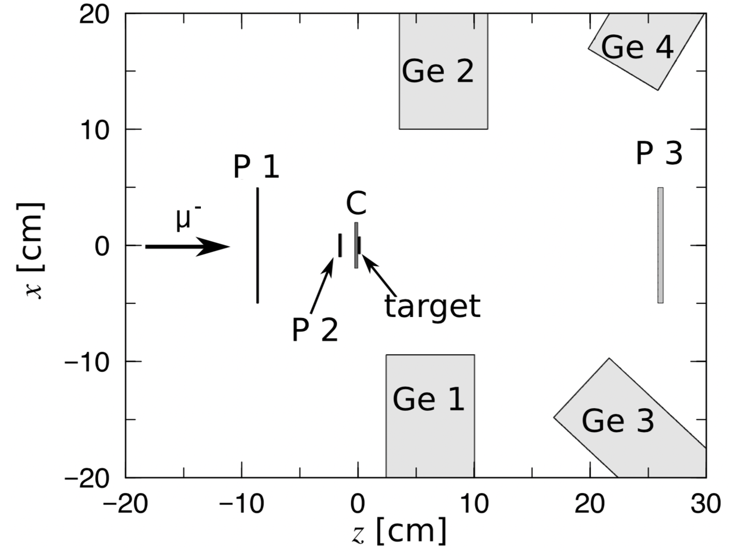
Figure 1: A top view of the detector configuration. The detectors are shown on the actual position and size, but the thickness of the upstream counters (P1 and P2) and the target are drawn thicker to see easily.

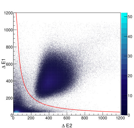
Figure 2: Particle identification with P1 and P2. The solid line represents the threshold value to discriminate the muon events from the electron events.

The muons and the electrons in the beam were identified by the energy loss at P1 and P2 because the muon deposits higher energy than the electron with the same momentum. Figure 2 shows a two-dimensional histogram of the energy deposits measured by P1 and P2. We adopted a threshold on the geometric mean of the QDC data of P1 and P2 to identify the muon as shown as the solid line in the figure. Some muons did not stop at the target and reached P3 since the effective area of P2 is larger than the size of the targets. The events containing any signals at P3 were eliminated from the following analysis.

After the muon stopped at the target, the muonic atom is formed, and muonic X rays are emitted at a prompt timing. The muon in the 1s orbit decays via $\mu$-$e$ decay or the muon capture with a lifetime of about 100 ns for the palladium. The highly excited nucleus is formed by the muon capture and emits nucleons and $\gamma$ rays. The X rays and the $\gamma$ rays can be separated by the photon detection timing. Figure 3 shows the photon detection time spectrum at the germanium detectors against the beam detection timing at P2 for $\mathrm{{}^{108}Pd}$. The prompt peak in the spectrum corresponds to the X ray, and the following exponential decay is originated from the $\gamma$ ray. The red solid curve in the figure is following function used to fit the spectrum:

$$f(t) =f_{X}(t)+f_{\gamma}(t)+C,$$ (1)

$$f_{X}(t) =A_{X}\exp\left(-\frac{t^{2}}{2\sigma_{T_{X}}^{2}}\right),$$ (2)

$$f_{\gamma}(t) =A^{\prime}_{\gamma}\exp\left(-\frac{t}{\tau}\right)\left[1-\mathrm{Erf}\left(\frac{(\sigma_{T_{\gamma}}^{2}/\tau)-t}{\sqrt{2}\sigma_{T_{\gamma}}}\right)\right],$$ (3)

where $C$ is the constant background term, $\mathrm{Erf}(x)$ is an error function, $\tau$ is the lifetime of the muonic palladium, and $\sigma_{X}$ and $\sigma_{\gamma}$ represent the timing resolutions of the germanium detectors averaged in the energy region of the X rays and $\gamma$ rays, respectively. The first term $f_{X}(t)$ is a Gaussian distribution of the X-ray timing, and the second term $f_{\gamma}(t)$ is the exponential decay curve convoluted by the Gaussian of the detector timing resolution. The decay constant of the timing spectra ($\lambda=1/\tau$) in the fitting function (1) corresponds to the lifetime of the muon in the 1s state of the muonic palladium. The obtained lifetimes of the palladium isotopes are summarized in Table 2. To obtain X-ray energy spectra, the photon timing is gated on the $\pm 3\sigma_{X}$ prompt region.

For the energy calibration of the germanium detectors, standard $\gamma$-ray sources of ${}^{60}\mathrm{Co}$, ${}^{133}\mathrm{Ba}$, ${}^{137}\mathrm{Cs}$ and ${}^{152}\mathrm{Eu}$ were used. In addition to these sources, background $\gamma$ peaks at 2223 keV from $p(n,\gamma)d$ reaction, 3539 keV from ${}^{28}\mathrm{Si}(n,\gamma)^{29}\mathrm{Si}$ reaction, 2754 keV from ${}^{27}\mathrm{Al}(n,\alpha)^{24}\mathrm{Na}$ reaction and 2615 keV of ${}^{208}\mathrm{Tl}$ decay were used for the energy calibration at the high energy region.

We report complete muonic X-ray transition energies up to $4f$-$3d$ transitions of five stable palladium isotopes for the first time. Figure 4 shows the X-ray energy spectrum for ${}^{108}\mathrm{Pd}$. The peaks were assigned to each muonic X-ray transition and fitted by a Gaussian function with a constant background term. The transition energies were obtained from the observed X-ray energies by applying the photon recoil correction of approximately 0.08 keV, in which the atom is kicked by the X ray and gains small kinematic energy. The transition energies ($E$) of each transition are summarized in Table 3 for even isotopes and Table 4 for ¹⁰⁵Pd. For ${}^{105}\mathrm{Pd}$, the $2p_{3/2}$-$1s_{1/2}$ transition has the hyperfine splitting, and it is impossible to estimate the detail peak structure due to the lack of resolution and statistics. The uncertainties in Table 3 and 4 include the statistical and systematic uncertainties. The systematic uncertainty on the energy is caused by the non-linearity of the ADC circuit and the gain drift of the germanium detectors during the experiment. Note that the statistical uncertainty is dominant for the $2p$-$1s$ transitions, while the systematic uncertainty is the major component for the other transitions. The $2p$-$1s$ transition energies appear in the compilations Fricke et al. (1995); Angeli and Marinova (2013), though the original paper was unpublished Hack (1989), and the obtained energies are consistent with the values in the compilation within the uncertainty.

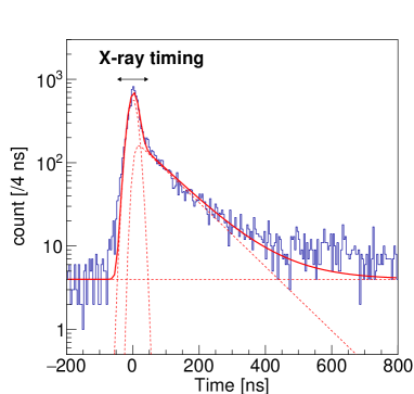
Figure 3: The timing spectrum of the photons after the muon irradiation to $\mathrm{{}^{108}Pd}$. The timing gate used for the X-ray spectrum is also shown. The red solid line represents the fitting function, Eq. (1), and the dotted lines are each component in the function. See text for detail.

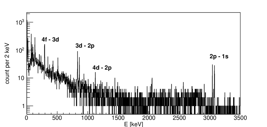
Figure 4: The entire spectrum of the $\mathrm{{}^{108}Pd}$ measurement gated on the X-ray timing. The intense peaks are indicated.

Table 2: The lifetimes ($\tau$) and the total capture rates ($\Lambda_{C}$) of muonic palladium determined in this work. Theoretical total capture rates are taken from Zinner et al. (Zinner et al., 2006) and Marketin et al. (Marketin et al., 2009). See text for detail of the calculation.

	$\tau$ [ns]	$\Lambda_{C}$ $[10^{6}~{}{\rm s^{-1}}]$	Zinner	Marketin
${}^{104}{\rm Pd}$	$87(3)$	$11.1(4)$	12.71	13.182
${}^{105}{\rm Pd}$	$109(7)$	$8.8(6)$	-	-
${}^{106}{\rm Pd}$	$97(7)$	$9.9(7)$	11.44	11.912
${}^{108}{\rm Pd}$	$109(4)$	$8.8(3)$	10.44	10.746
${}^{110}{\rm Pd}$	$102(6)$	$9.4(6)$	9.607	9.821

Table 3: Muonic X-ray transition energies for even palladium isotopes. The Fermi parameters $c$ and $t$ determined by the transition energies are also listed. The Fermi parameters $c$ in the reference which is determined with fixed $t=2.3$ fm are also shown. The Barrett parameters $k$,$\alpha_{B}$, and $R_{k\alpha_{B}}$ are also listed.

Nuclei	X-ray energies		Charge parameters from present experiment						Reference Fricke et al. (1995)
	transition	$E$ [keV]	$k$	$\alpha_{B}$ [fm-1]	$R_{k\alpha_{B}}$ [fm]	$c$ [fm]	$t$ [fm]	rms [fm]	$c$ [fm]	rms [fm]
104Pd	$2p_{1/2}$-$1s_{1/2}$	3057.8(3)	2.163	0.1037	5.762(2)	5.26(12)	2.25(25)	4.493${}_{-7}^{+28}$	5.2509(4)	4.509
	$2p_{3/2}$-$1s_{1/2}$	3091.7(2)	2.145	0.1013	5.764(2)
	$3d_{5/2}$-$2p_{3/2}$	833.4(1)	3.705	0.0802	5.91(2)
	$3d_{3/2}$-$2p_{1/2}$	863.6(3)	3.798	0.1183	5.89(4)
	$4d_{5/2}$-$2p_{3/2}$	1122.5(6)	3.703	0.0795	5.9(1)
	$4f_{7/2}$-$3d_{5/2}$	291.6(1)	5.864	0.1257	6.1(4)
	$4f_{5/2}$-$3d_{3/2}$	294.9(2)	6.252	0.0963	6.3(6)
106Pd	$2p_{1/2}$-$1s_{1/2}$	3050.3(5)	2.157	0.1027	5.792(2)	5.49(30)	1.76(65)	4.507${}_{-5}^{+96}$	5.2847(2)	4.532
	$2p_{3/2}$-$1s_{1/2}$	3084.0(3)	2.148	0.1013	5.795(2)
	$3d_{5/2}$-$2p_{3/2}$	833.4(3)	3.705	0.0802	5.92(7)
	$3d_{3/2}$-$2p_{1/2}$	863.8(3)	3.798	0.1184	5.86(4)
	$4d_{5/2}$-$2p_{3/2}$	1124.8(4)	3.703	0.0795	5.77(9)
	$4f_{7/2}$-$3d_{5/2}$	291.7(2)	5.864	0.1257	5.6(7)
	$4f_{5/2}$-$3d_{3/2}$	295.1(3)	6.251	0.0963	5.6(8)
108Pd	$2p_{1/2}$-$1s_{1/2}$	3042.9(2)	2.153	0.1020	5.822(2)	5.45(11)	1.96(27)	4.537${}_{-6}^{+27}$	5.3184(2)	4.556
	$2p_{3/2}$-$1s_{1/2}$	3076.6(2)	2.149	0.1012	5.824(2)
	$3d_{5/2}$-$2p_{3/2}$	833.3(1)	3.705	0.0799	5.95(2)
	$3d_{3/2}$-$2p_{1/2}$	863.5(1)	3.798	0.1184	5.91(1)
	$4d_{5/2}$-$2p_{3/2}$	1124.4(3)	3.702	0.0793	5.87(7)
	$4f_{7/2}$-$3d_{5/2}$	291.6(1)	5.864	0.1257	5.8(3)
	$4f_{5/2}$-$3d_{3/2}$	294.9(1)	6.252	0.0963	6.3(3)
110Pd	$2p_{1/2}$-$1s_{1/2}$	3036.2(7)	2.149	0.1013	5.849(3)	5.60(26)	1.61(70)	4.548${}_{-6}^{+100}$	5.3490(3)	4.577
	$2p_{3/2}$-$1s_{1/2}$	3068.8(4)	2.153	0.1013	5.856(2)
	$3d_{5/2}$-$2p_{3/2}$	833.4(2)	3.704	0.0799	5.94(5)
	$3d_{3/2}$-$2p_{1/2}$	863.4(3)	3.798	0.1184	5.92(4)
	$4d_{5/2}$-$2p_{3/2}$	1124.2(5)	3.702	0.0793	5.9(1)
	$4f_{7/2}$-$3d_{5/2}$	291.6(1)	5.864	0.1257	6.1(4)
	$4f_{5/2}$-$3d_{3/2}$	294.9(2)	6.252	0.0963	6.3(8)

Table 4: Muonic X-ray transition energies for ¹⁰⁵Pd.

X-ray energies
transition	E [keV]
$2p_{1/2}$-$1s_{1/2}$	3054.9(5)
$2p_{3/2}$-$1s_{1/2}$	3091.5(8)
$3d_{5/2}$-$2p_{3/2}$	832.3(3)
$3d_{3/2}$-$2p_{1/2}$	864.5(3)
$4f_{7/2}$-$3d_{5/2}$	291.4(2)
$4f_{5/2}$-$3d_{3/2}$	294.9(6)

III Total muon capture rate

The total capture rate of the nuclear muon capture ($\Lambda_{c}$) corresponds to the lifetime of the muonic 1s state ($\tau$) with the following relation:

$$\frac{1}{\tau}=\Lambda_{C}+Q\frac{1}{\tau_{\mu^{+}}},$$ (4)

where $\tau_{\mu^{+}}$ is the lifetime of a positive muon (2.1969811(22) $\mu$s) Olive et al. (2014) and $Q$ is the Huff factor. The Huff factor is $Q=0.927$ for palladium (Suzuki et al., 1987; Blair et al., 1962).

The total muon capture rates deduced from the measured lifetimes are listed in Table 2 for each palladium isotope. In the fitting procedure, we assume the lifetimes of excited states in each rhodium isotope produced by the muon capture are negligibly small. If the excited states have longer lifetimes, the measured $\tau$ become longer and, hence, $\tau$ in Table 2 are the upper limits. Consequently, the determined capture rates $\Lambda_{C}$ here are the lower limits.

For a consistency check, the lifetime of natural palladium was calculated by summing up the measured decay curves with the weight of the natural abundance of palladium. Natural palladium contains 1.02% of $\mathrm{{}^{102}Pd}$ and the existence of $\mathrm{{}^{102}Pd}$ is neglected here. The lifetime of this summed-up decay curve is $102\pm 8$ ns, which is consistent with the previously measured value $96\pm 0.6$ ns (Eckhause et al., 1966) of the natural palladium within the uncertainty.

The nuclear muon capture changes a proton into a neutron in the excited states. The excited states after the nuclear muon capture can be well described by the random phase approximation (RPA), in which each excited state is written as a superposition of one-particle-one-hole state. The theoretical calculation of $\Lambda_{C}$ is also listed in Table 2 with RPA based on single-particle states generated by Woods-Saxon potential by Zinner et al. (Zinner et al., 2006) and the relativistic proton-neutron quasiparticle random phase approximation (pn-RQRPA) using the relativistic Hartree-Bogoliubov basis by Marketin et al. (Marketin et al., 2009). Both the experimental and theoretical values have a decreasing trend along with the mass number $A$. Theoretical values, however, overestimate $\Lambda_{C}$ for all palladium isotopes compared with the experimental results. Further experimental and theoretical studies are required.

IV Discussion I: Nuclear Charge Radius

In this section, the nuclear charge radii of the palladium isotopes are deduced from the measured muonic transition energies. The two-parameter Fermi (2pF) function is assumed as the charge distribution in the analysis. Once the 2pF function is assumed, the two parameters in the 2pF function are determined using the experimental inputs, and then the rms charge radius can be calculated from the 2pF function.

Here we will follow references Barrett (1974); Borie and Rinker (1982); Michel et al. (2017). One can start from a simple two-body bound system with the muon and the nucleus in their center-of-mass system using their reduced mass ($m_{r}$). Omitting the nuclear excitation, the Hamiltonian of the muonic atom can be written as

$$H=H_{\mu}+H_{\mu-N},$$ (5)

where $H_{\mu}$ is the free Dirac Hamiltonian with the reduced mass ($m_{r}$) and $H_{\mu-N}$ is the interaction Hamiltonian. Considering the ground state of a spherical even-even nucleus with the spin parity $0^{+}$, $H_{\mu-N}$ contains only the static electric part. The interaction Hamiltonian can be expressed with the fine structure constant $\alpha$ and the nuclear charge distribution $\rho(r)$ as

$$H_{\mu-N}=-\alpha\int\frac{\rho(r^{\prime})}{|r-r^{\prime}|}\mathrm{d}r^{\prime},$$ (6)

where $\rho(r)$ must be normalized to be $\int\rho\mathrm{d}r^{3}=Z$. For the $0^{+}$ states, the static potential with the spherical charge distribution (Eq. (6)) is also adequate for deformed nuclei as the first approximation. This approximation is also justified for deformed nuclei considering a time-averaged distribution.

For the numerical calculation, one must assume the functional form of $\rho(r)$. The 2pF distribution with parameters $c$ and $t$ is used in this analysis:

$$\rho_{\mathrm{2pF}}(r)=\frac{N_{0}}{1+\exp{[\frac{(r-c)}{t/(4\ln{3})}]}},$$ (7)

where $N_{0}$ is the normalization factor. The Fermi parameters, $c$ and $t$, are the half-density radius and the diffuseness, respectively. Once the functional form of $\rho(r)$ is given, the binding energies of the muonic atom are calculated by numerically solving the eigenvalue problem of the Hamiltonian (Eq. (5)). The muonic X-ray transition energies are then calculated to be the difference of the binding energies between the two corresponding states.

For further correction, the QED and recoil corrections should be included in the bare wavefunctions and binding energy of Eq. (5) as same as an ordinal electronic atom. For the muonic atom, the electron screening effect by the inner shell electrons should also be taken into account. We include these perturbative corrections following Ref. Michel et al. (2017).

In addition to the above corrections, an energy shift by nuclear polarization and self-energy correction should also be considered. The binding energy of the muonic atom reaches several MeV, which is comparable with the nuclear excitation energy. The coupling between the nuclear structure and the muonic atomic states causes an energy shift by several keV in the binding energy. This energy shift is called a nuclear polarization effect. Complete calculation of the nuclear polarization correction is almost impossible because all excited states in the nucleus contribute to the energy shift. The energy shift by the nuclear polarization is estimated to be about 1.4 keV for $2p$-$1s$ transitions for the palladium isotopes Fricke et al. (1995). The energy shift by the self-energy correction is relatively smaller than the electronic atom and estimated to be the order of 1 keV for the $1s$ state Cheng et al. (1978). The nuclear polarization effect and self-energy correction are not included in the present analysis.

\begin{overpic}[width=199.16928pt]{./figure/Band_forpaper.pdf} \put(50.0,90.0){\large(a)} \end{overpic}

\begin{overpic}[width=199.16928pt]{./figure/Fermi2Derror_witht23line.pdf} \put(50.0,90.0){\large(b)} \end{overpic}

Figure 5: (a) 1$\sigma$ region limited by the obtained muonic transition energies in the two-dimensional $c$-$t$ space for ¹⁰⁸Pd. Each shaded area corresponds to limited region by each muonic transition with 1$\sigma$ uncertainty. (b) 1$\sigma$ uncertainty region of the Fermi parameter in the $c$-$t$ space for ${}^{108}{\rm Pd}$. The red star symbol shows the determined Fermi parameters which gives the $\chi^{2}$ minimum. The red and blue ellipses represent the region for $\chi^{2}=\chi^{2}_{\mathrm{min}}+1$ and $\chi^{2}=\chi^{2}_{\mathrm{min}}+2.3$, respectively. The contours of the rms radii (0.1 fm interval) are illustrated with the black solid lines. The black dotted line represents $t=2.3$ fm.

To obtain the Fermi parameters, the theoretically calculated transition energies were fit to the experimental transition energy through the $\chi^{2}$ minimization procedure. It would be an important note that single transition energy is only able to limit the two-dimensional $c$-$t$ parameter space ($c$-$t$ space) as a belt-like area corresponding to its experimental uncertainty, as shown in Fig. 5-(a). The combination of more than two areas with different gradients in the $c$-$t$ space is required to determine the pair of the Fermi parameters. It is thus necessary to include the higher transitions adding to the lowest transitions $2p_{1/2}$-$1s_{1/2}$ and $2p_{3/2}$-$1s_{1/2}$ since these lowest two transitions are completely overlapped to be distinguished. Therefore, we include four observed transitions, $2p_{1/2}$-$1s_{1/2}$, $2p_{3/2}$-$1s_{1/2}$, $3d_{3/2}$-$2p_{1/2}$ and $3d_{5/2}$-$2p_{3/2}$, to the minimization procedure. The other transitions were not used because of their low statistics. The parameters $c$ and $t$ were scanned independently to find minimum $\chi^{2}$ value ($\chi^{2}_{\mathrm{min}}$) in the $c$-$t$ space. The determined Fermi parameters are summarized in Table 3 together with their uncertainty.

The rms radii were calculated as the square root of the second-order nuclear moment from the obtained parameters;

$$\mathrm{(rms)}^{2}=\langle r^{2}\rangle=\int\rho_{\mathrm{2pF}}(r)4\pi r^{2}\mathrm{d}r.$$ (8)

The deduced rms radii for the palladium isotopes are listed in Table 3. The 1$\sigma$ uncertainty region, namely the region in which the $\chi^{2}$ value is less than $\chi^{2}_{\mathrm{min}}+1$ for one parameter and $\chi^{2}_{\mathrm{min}}+2.3$ for two parameters, in the $c$-$t$ space is illustrated for ¹⁰⁸Pd in Fig. 5-(b). The uncertainties quoted for the Fermi parameters are taken from $\chi^{2}_{\mathrm{min}}+1$ region and the uncertainties for rms radii are estimated using $\chi^{2}_{\mathrm{min}}+2.3$ region. The uncertainty quoted for the rms radii in Table 3 is relatively small compared to that for the Fermi parameters. This is because the sensitivity of the X-ray energies to the rms radius is higher than that of the Fermi parameters. The high sensitivity to the rms radius is indicated by the fact that the experimental 1$\sigma$ region has a similar slope to the contour of the rms radius as shown in Fig. 5-(b). The transition energy of the $2p$-$1s$ transitions is sensitive to rms radius, not to the Fermi parameters $c$ and $t$.

The Fermi parameters and the rms radii listed in the compilation are incorporated in Table 3. The Fermi parameter $c$ in the reference Fricke et al. (1995) seems much higher precision than the present results. This discrepancy is due to the different approaches used in the interpretation. In our interpretation, two Fermi parameters ($c$ and $t$) are treated as free parameters and determined by the measured X-ray energies including higher transitions. In the compilation, $c$ is deduced from only the $2p$-$1s$ transitions with the assumption of the fixed $t$ value as 2.3 fm. The fixed $t$ value is an empirical value based on the systematics. This assumption corresponds to the projection to the $t$ one-dimensional space at $t=2.3$ in Fig. 5-(b) and leads the extremely small uncertainty. It should be noted that no uncertainty for the rms radii is given in the compilation because of the difficulty in the estimation of the systematic uncertainty from the fixed $t$ value. Regardless of the different approaches, the rms radii obtained by the present work and the compilation are consistent within our uncertainty.

We can now discuss the accuracy of the rms radius since the uncertainty on the rms radius is obtained. In the present analysis, the uncertainty of the rms radius is limited by the experimental uncertainty of the $3d$-$2p$ transition energies. The accuracy of the rms radius from each transition is corresponding to the width of the belt-like area in Fig. 5-(a). The accuracy of the rms radius from the $2p$-$1s$ transitions is higher than that from the $3d$-$2p$ transitions by about ten times. It should be noted that the experimental uncertainty of the transition energies differs only twice for these transitions, namely 0.0066% ($0.2$ keV for $3043$-keV X ray) and 0.012% ($0.1$ keV for $833$-keV X ray) for the $2p$-$1s$ and $3d$-$2p$ transitions, respectively. The difference of the accuracy is thus from the difference of the intrinsic sensitivity for the nuclear charge radius: the change of the nuclear charge distribution affects the $2p$-$1s$ transition energy more drastically than thee $3d$-$2p$ transitions since the former occurs closer to the nucleus than the latter. In general, the higher transitions have less intrinsic sensitivity for the nuclear charge radius. In order to compensate for the less intrinsic sensitivity, the energies of the $3d$-$2p$ transitions must be determined more precisely than those of the $2p$-$1s$ transitions for the accurate determination of the rms radius. It should be mentioned again that the experimental uncertainty of the $3d$-$2p$ transition energies are dominated by the systematic uncertainty, not from the statistical uncertainty. For a future experiment, it is thus important to employ the sophisticated detector system to reduce the systematic uncertainty caused by the gain drift of the detector and the non-linearity of the circuit.

V Discussion II: Nuclear Charge Distribution

We now discuss the nuclear charge distribution using the muonic transition energies in this section. The major concern of the approach with the 2pF distribution is the limitation of the functional form. Generally, the actual nuclear charge distribution $\rho(r)$ is complicated and has a non-analytic form, and any approach assuming a certain functional form must contain the limitation. Thus, we employ the Barrett model, which is sometimes referred to as the ”model-independent” approach and is motivated to treat the nuclear distribution without any functional assumptions Barrett (1970). In the Barrett model, a certain nuclear moment, called Barrett moment, is derived as the perturbation from the distribution with an analytic functional form. For the derivation of the Barrett moment, we will follow Refs. Barrett (1970); Ford and Rinker (1973); Angeli (2002); Engfer et al. (1974); Fricke et al. (1995).

Let us consider a reference nuclear charge distribution $\rho_{0}(r)$ which is close to $\rho(r)$. $\rho_{0}(r)$ should be an analytic form to calculate the binding energy and wavefunctions, and fulfill the following normalization; $\int\rho(r)\mathrm{d}^{3}r=\int\rho_{0}(r)\mathrm{d}^{3}r=Z$. The muonic transition energy $E_{ij}[\rho]$ is the energy difference from the initial state $i$ to the final state $j$ and depends on the charge distribution $\rho(r)$. In the first-order perturbation, the difference of the transition energies caused by the change of the charge distribution $\delta\rho(r)=\rho(r)-\rho_{0}(r)$ can be approximated as

$$\delta E =E_{ij}[\rho]-E_{ij}[\rho_{0}]$$

$$=\int\delta\rho(r)\Delta V_{ij}(r)4\pi r^{2}\mathrm{d}r.$$ (9)

$\Delta V_{ij}(r)=V_{i}(r)-V_{j}(r)$, where $V_{ij}(r)$ are the Coulomb potential of the muon at the state $i$ and $j$, can be written as

$$\Delta V_{ij}(r)=\alpha\int\frac{\psi_{i}^{\dagger}(r^{\prime})\psi_{i}(r^{\prime})-\psi_{j}^{\dagger}(r^{\prime})\psi_{j}(r^{\prime})}{|r^{\prime}-r|}4\pi r^{2}\mathrm{d}r$$ (10)

using the muon wavefunctions $\psi_{i}(r)$ in each atomic state. This treatment has also been applied for the analysis of isotope or isomeric shifts as considering $\delta\rho(r)$ as the distribution difference between the nuclei. In this paper, $\delta\rho(r)$ always represents the difference between the reference distribution $\rho_{0}(r)$ and the actual distribution $\rho(r)$.

For further simplification, $\Delta V_{ij}(r)$ is approximated with an analytic function. Barrett proposed a phenomenological functional form

$$\Delta V_{ij}(r)\simeq A+Br^{k}e^{-\alpha_{B}r}$$ (11)

with four parameters $k$, $\alpha_{B}$, $A$ and $B$. The $\alpha_{B}$ is denoted with $\alpha$ in the references Barrett (1970); Ford and Rinker (1973); Angeli (2002); Engfer et al. (1974); Fricke et al. (1995) and we use $\alpha_{B}$ in this paper to discern it from the fine-structure constant $\alpha$. The form Eq. (11) is only valid in the limited region with $r<10$-$20$ fm for typical cases and the product $\delta\rho(r)\Delta V_{ij}(r)$ become zero for large $r$. One can assume $\rho(r)$ and $\rho_{0}(r)$ give same $k$, $\alpha_{B}$, $A$, and $B$ as long as $\delta\rho(r)$ is small. Then these parameters are independent of the choice of the reference distribution $\rho_{0}(r)$. We can obtain the parameters by fitting Eq. (11) to the $\Delta V_{ij}(r)$ calculated using Eq. (10) with assumed $\rho_{0}(r)$. Note that the parameters are different among the transitions even in the same nucleus. Since $\delta\rho(r)$ is normalized to $\int\delta\rho(r)4\pi r^{2}\mathrm{d}^{3}r=0$, the constant term $A$ has no effect in the discussion below.

Using the parameters in (11), the Barrett moment $\langle r^{k}e^{-\alpha_{B}r}\rangle$ can be defined as

$$\langle r^{k}e^{-\alpha_{B}r}\rangle=\frac{1}{Z}\int\rho(r)r^{k}e^{-\alpha_{B}r}4\pi r^{2}\mathrm{d}r.$$ (12)

Now the energy difference Eq. (9) can be expressed as

$$\delta E=ZB[\langle r^{k}e^{-\alpha_{B}r}\rangle-\langle r^{k}e^{-\alpha_{B}r}\rangle_{0}],$$ (13)

where $\langle r^{k}e^{-\alpha_{B}r}\rangle_{0}$ denotes the Barrett moment with $\rho_{0}$. Furthermore, the Barrett equivalent radius $R_{k\alpha_{B}}$ is introduced as follows:

$$\frac{3}{R_{k\alpha_{B}}^{3}}\int_{0}^{R_{k\alpha_{B}}}r^{k}e^{-\alpha_{B}r}r^{2}\mathrm{d}r=\langle r^{k}e^{-\alpha_{B}r}\rangle.$$ (14)

In this approach, derivation of the rms radius is difficult, and the equivalent radius is generally used for the comparison among the experimental results from the measurements of the muonic X rays. The equivalent radius is independent of the parameter $B$ and only depends on $k$ and $\alpha_{B}$. To determine the experimental $R_{k\alpha_{B}}$, the first-order form

$$\delta R_{k\alpha_{B}}=C_{Z}\delta E$$ (15)

can be used. The correction factor $C_{Z}$ is given by

$$C_{Z}=\frac{R_{k\alpha_{B}}}{3ZB[\langle r^{k}e^{-\alpha_{B}r}\rangle_{0}-R_{k\alpha_{B}}^{k}e^{-\alpha_{B}R_{k\alpha_{B}}}]}$$ (16)

with the equivalent radius $R_{k\alpha_{B}}$ that is calculated based on $\rho_{0}(r)$.

In Table 3, calculated $k$, $\alpha_{B}$, and $R_{k\alpha_{B}}$ using $\rho_{0}(r)=\rho_{\mathrm{2pF}}(r)$ with the obtained Fermi parameters in Sec. IV are shown. The QED, recoil, and electron screening corrections were included in this calculation. For the uncertainty of $R_{k\alpha_{B}}$, the first-order form Eq. (15) is combined with the experimental uncertainty except for the $4f$-$3d$ transitions. Because the experimental uncertainty is too large for the $4f$-$3d$ transitions to justify the first-order approximation, the uncertainty for these transitions is estimated by scanning the Fermi parameters within the experimental uncertainty and taking a conservative value.

\begin{overpic}[width=199.16928pt]{./figure/Barrett_systematics_final2.pdf} \put(50.0,90.0){\large(a)} \end{overpic}

\begin{overpic}[width=199.16928pt]{./figure/Barrett_manyRhos_final2.pdf} \put(50.0,90.0){\large(b)} \end{overpic}

Figure 6: (a) Barrett equivalent radii for each index $k$. (b) Nuclear charge distribution with different functional forms for $\mathrm{{}^{108}Pd}$. The black solid lines are 2pF distribution, the blue dashed lines are the theoretical calculation from HF-BCS and the red dotted lines are from the electron scattering experiment.

The physical interpretation of the Barrett model becomes clear by comparing it with the ordinary nuclear moments. In Barrett’s approach, the equivalent radius $R_{k\alpha_{B}}$ can be determined for each $k$ and $\alpha_{B}$ while the rms radius is not obtained. Considering the obtained $\alpha_{B}$ in Table 3 is almost constant around $0.1$ for all transitions, let us simplify to be $\alpha_{B}=0$. Under this simplification, the Barrett moment (Eq. (12)) is now a $k$-th nuclear moment with a non-integer order index. The index $k$ increases from $2$ to $6$ as the transitions go higher, and the $k$-th nuclear moments are estimated for each transition. Thus, the measurement of the higher transitions provides information on the higher nuclear moments. Furthermore, the simplified Barrett moments provide a clear view of the benefits of the higher transitions to determine the charge parameters of the 2pF function discussed in Sect. IV. The variety of the nuclear moments given by Barrett’s approach corresponds to the difference in the gradient of the 1$\sigma$ region in Fig. 5-(a). Therefore, two $2p$-$1s$ transitions with similar $k$ give the similar gradients in Fig. 5-(a) and the $3d$-$2p$ transitions with $k\neq 2$ help to limit the $c$-$t$ space of the 2pF distribution.

The $k$-dependence of the equivalent radius can be used to discuss the general functional forms of the charge distribution since the discussion of the equivalent radii is now not limited to 2pF. Figure 6-(a) shows the measured equivalent radii for ${\rm{}^{108}Pd}$ for the $2p$-$1s$ and $3d$-$2p$ transitions as a function of $k$. Hereafter, let us assume $\alpha_{B}$ is constant among the transitions and use the averaged value of two $2p$-$1s$ transitions as $\alpha_{B}$. Once a functional form of the charge distribution is given, one can calculate the equivalent radii corresponding to the charge distribution for any $k$ and draw the curve in this $k$-$R_{k\alpha}$ space as shown in Fig. 6-(a). The lines drawn in Fig. 6-(a) represent the equivalent radius lines corresponding to the three charge distributions shown in Fig. 6-(b). The black solid lines in the figures represent 2pF with the Fermi parameters in Table 3. Since this 2pF is considered as the non-perturbative distribution $\rho_{0}(r)$ in this treatment, this agreement just indicates self-consistency in the present analysis. The blue dashed lines are a Hartree-Fock calculation with BCS basis (HF-BCS) InP ; Ebata et al. (2014); Ebata and Nakatsukasa (2017), and the red dotted lines represent the electron scattering experiment Laan (1986). All of the charge distribution fulfill the normalization of $\int\rho(r)4\pi r^{2}\mathrm{d}r=Z$.

Using Barrett’s approach, one can compare the muonic X-ray transition energies with the given charge distribution in the $k$-$R_{k\alpha_{B}}$ space. The blue dashed lines in Fig. 6 show the theoretical calculation using HF-BCS with 3D Skyrme force. Since the original reference provides the density distribution of the point proton, the charge distribution is calculated by folding with the Gaussian proton charge distribution Kurasawa and Suzuki (2019). The theoretical distribution gives the rms charge radius of 4.55 fm, which is consistent with that obtained value of 4.537${}_{-6}^{+27}$ fm in the present study. This consistency in the rms radius corresponds to the agreement in the equivalent radii for the $2p$-$1s$ transitions in Fig. 6-(a) since the Barrett moments at $k\sim 2$ is very similar to the second order nuclear moment, namely the $\langle r^{2}\rangle=(\mathrm{rms})^{2}$. On the contrary, the theoretical calculation overestimates the Barrett moments at the $3d$-$2p$ transitions at $k\sim 3.7$. It indicates that the theoretical calculation fails to reproduce the higher moment in spite of the agreement on the rms radius. The present example demonstrates that the measurement of the higher transitions provides a further constraint to the theoretical calculations.

The red dotted line in Fig. 6-(b) is the charge distribution obtained from the electron scattering for the ${}^{108}\mathrm{Pd}$ De Vries et al. (1987); Laan (1986). As shown in Fig. 6-(a), the equivalent radii obtained from the present X-ray measurement agree with those from the electron scattering for the $3d$-$2p$ transitions at $k\sim 3.7$. On the other hand, our equivalent radii are larger than those from the electron scattering for the $2p$-$1s$ transitions at $k\sim 2$. It reflects the slightly larger rms radius of 4.537${}_{-6}^{+27}$ fm obtained from the muonic X-ray spectroscopy than 4.524(10) fm from the electron scattering. Note that two independent measurements provide almost the same accuracy on the rms radius. As discussed in Sect. IV, the uncertainty of the rms radius is dominated by that of the $3d$-$2p$ transition energies. The uncertainty of the equivalent radii for the $2p$-$1s$ transitions is thus smaller than that of the rms radius. Since the equivalent radii are linked to the individual muonic transitions while the rms radius is deduced by combining several transitions in the present analysis, the $k$-$R_{k\alpha_{B}}$ space provides a direct comparison among the different experimental data. Although the quantitative discussion is difficult because the uncertainty of the distribution of the electron scattering is not given in the reference, the discrepancy is probably due to the difference in the sensitivity to the charge distribution between the two methods. The scattering experiment usually quotes larger uncertainty for the inner part of the distribution because the experimental uncertainty is larger for the larger momentum transfer. Contrary, the muonic transition energies have the smallest uncertainty for the $k\sim 2$, namely the $2p$-$1s$ transitions, and thus it is rather sensitive to the center of the distribution. Therefore, two experimental methods, the muonic X-ray spectroscopy and the electron scattering, are complementary to discuss the charge distribution.

We have demonstrated the muonic transition energies constrain the nuclear charge distribution through the $k$-$R_{k\alpha_{B}}$ plot. In the present work, the systematic comparison along the index $k$ is limited by the experimental uncertainty of the $3d$-$2p$ transition energy as similar to the derivation of the rms radius discussed in Sect. IV. For further constraints on the charge distribution from the muonic X-ray spectroscopy, observations of the X-ray series with $k$ are required, which were not observed in the present experiment because of the limited statistics. As $k$ represents the order index of Barret’s moments, higher series of the muonic X-ray, such as $4f$-$3d$ at $k\sim 6$, restricts a higher moment, namely the outer region of the charge distribution. Furthermore, the transitions with smaller $k$, such as $2s$-$2p$ at $k\sim 1.5$, for example, are particularly of interest. The transition energies with small $k$ constrain the inner part of the distribution, which is difficult to investigate with the electron scattering. The inner part of the nuclear charge distribution will be discussed in the future high-statistics measurements using the $k$-$R_{k\alpha_{B}}$ plot.

VI Conclusion

The muonic X-ray spectroscopy was performed at MuSIC-M1 beamline at Research Center for Nuclear Physics (RCNP), Osaka University. The muonic X-ray energies were measured up to the $4f$-$3d$ transitions for stable palladium isotopes with $A=104$, $105$, $106$, $108$ and $110$. The analysis method to deduce the root-mean-square (rms) charge radius from the muonic transition energies is proposed. By combining the $2p$-$1s$ and $3d$-$2p$ transition energies, two parameters in the two-parameter Fermi (2pF) distribution are simultaneously deduced and the rms radius is obtained with the experimental uncertainty. The charge distribution of the nucleus is discussed employing the Barrett model. The $k$-$R_{k\alpha_{B}}$ plot provides a direct comparison between the muonic transition energies and the charge distribution resulting from the electron scattering and the theoretical calculations.

References

- Fricke et al. (1995) G. Fricke, C. Bernhardt, K. Heilig, L. A. Schaller, L. Schellenberg, E. B. Shera, and C. W. de Jjager, Atomic Data and Nuclear Data Tables 60, 177 (1995).
- Angeli and Marinova (2013) I. Angeli and K. Marinova, Atomic Data and Nuclear Data Tables 99, 69 (2013).
- Wakasugi et al. (2013) M. Wakasugi et al., Proceedings, 16th International Conference on Electromagnetic Isotope Separators and Techniques Related to their Applications (EMIS 2012): Matsue, Japan, December 2-7, 2012, Nucl. Instrum. Meth. B317, 668 (2013).
- Suda and Simon (2017) T. Suda and H. Simon, Progress in Particle and Nuclear Physics 96, 1 (2017).
- Tsukada et al. (2017) K. Tsukada, A. Enokizono, T. Ohnishi, K. Adachi, T. Fujita, M. Hara, M. Hori, T. Hori, S. Ichikawa, K. Kurita, K. Matsuda, T. Suda, T. Tamae, M. Togasaki, M. Wakasugi, M. Watanabe, and K. Yamada, Phys. Rev. Lett. 118, 262501 (2017).
- Terashima et al. (2008) S. Terashima, H. Sakaguchi, H. Takeda, T. Ishikawa, M. Itoh, T. Kawabata, T. Murakami, M. Uchida, Y. Yasuda, M. Yosoi, J. Zenihiro, H. P. Yoshida, T. Noro, T. Ishida, S. Asaji, and T. Yonemura, Phys. Rev. C 77, 024317 (2008).
- Zenihiro et al. (2010) J. Zenihiro, H. Sakaguchi, T. Murakami, M. Yosoi, Y. Yasuda, S. Terashima, Y. Iwao, H. Takeda, M. Itoh, H. P. Yoshida, and M. Uchida, Phys. Rev. C 82, 044611 (2010).
- Bergem et al. (1988) P. Bergem, G. Piller, A. Rueetschi, L. A. Schaller, L. Schellenberg, and H. Schneuwly, Phys. Rev. C 37, 2821 (1988).
- Barrett (1970) R. Barrett, Physics Letters B 33, 388 (1970).
- Strasser et al. (2005) P. Strasser, K. Nagamine, T. Matsuzaki, K. Ishida, Y. Matsuda, and M. Iwasaki, Nuclear Physics B - Proceedings Supplements 149, 390 (2005), nuFact04.
- Strasser et al. (2009) P. Strasser, A. Taniguchi, T. Matsuzaki, K. Ishida, Y. Matsuda, S. Ohya, M. Iwasaki, and K. Nagamine, Hyperfine Interactions 193, 121 (2009).
- Engfer et al. (1974) R. Engfer, H. Schneuwly, J. Vuilleumier, H. Walter, and A. Zehnder, Atomic Data and Nuclear Data Tables 14, 509 (1974), nuclear Charge and Moment Distributions.
- Hack (1989) T. Hack, Diploma thesis, Ph.D. thesis, Institüt fur Kernphysik, KPH 10/89, Universitäte Mainz (1989).
- Measday (2001) D. F. Measday, Physics Reports 354, 243 (2001).
- Primakoff (1959) H. Primakoff, Rev. Mod. Phys. 31, 802 (1959).
- Kolbe et al. (2000) E. Kolbe, K. Langanke, and P. Vogel, Phys. Rev. C 62, 055502 (2000).
- Zinner et al. (2006) N. T. Zinner, K. Langanke, and P. Vogel, Phys. Rev. C 74, 024326 (2006).
- Marketin et al. (2009) T. Marketin, N. Paar, T. Nikšić, and D. Vretenar, Phys. Rev. C 79, 054323 (2009).
- Terada et al. (2015) K. Terada, T. Katabuchi, M. Mizumoto, T. Arai, T. Saito, M. Igashira, K. Hirose, S. Nakamura, A. Kimura, H. Harada, J. Hori, K. Kino, and Y. Kiyanagi, Progress in Nuclear Energy 82, 118 (2015), selected Papers from the Fourth International Symposium on Innovative Nuclear Energy Systems, INES-4 - Innovative Nuclear Science and Technology Post Fukushima - held at Ookayama campus of Tokyo Institute of Technology.
- Cook et al. (2017) S. Cook, R. D’Arcy, A. Edmonds, M. Fukuda, K. Hatanaka, Y. Hino, Y. Kuno, M. Lancaster, Y. Mori, T. Ogitsu, H. Sakamoto, A. Sato, N. H. Tran, N. M. Truong, M. Wing, A. Yamamoto, and M. Yoshida, Phys. Rev. Accel. Beams 20, 030101 (2017).
- (21) D. Tomono and A. Sato, “Private communication,” .
- Baba et al. (2010) H. Baba, T. Ichihara, T. Ohnishi, S. Takeuchi, K. Yoshida, Y. Watanabe, S. Ota, and S. Shimoura, Nuclear Instruments and Methods in Physics Research Section A: Accelerators, Spectrometers, Detectors and Associated Equipment 616, 65 (2010).
- Olive et al. (2014) K. A. Olive et al. (Particle Data Group), Chin. Phys. C38, 090001 (2014).
- Suzuki et al. (1987) T. Suzuki, D. F. Measday, and J. P. Roalsvig, Physical Review C 35, 2212 (1987).
- Blair et al. (1962) I. Blair, H. Muirhead, T. Woodhead, and J. Woulds, Proceedings of the Physical Society 80, 938 (1962).
- Eckhause et al. (1966) M. Eckhause, R. T. Siegel, R. E. Welsh, and T. A. Filippas, Nuclear Physics 81, 575 (1966).
- Barrett (1974) R. C. Barrett, Reports on Progress in Physics 37, 1 (1974).
- Borie and Rinker (1982) E. Borie and G. A. Rinker, Rev. Mod. Phys. 54, 67 (1982).
- Michel et al. (2017) N. Michel, N. S. Oreshkina, and C. H. Keitel, Phys. Rev. A 96, 032510 (2017).
- Cheng et al. (1978) K. T. Cheng, W. D. Sepp, W. R. Johnson, and B. Fricke, Phys. Rev. A 17, 489 (1978).
- Ford and Rinker (1973) K. W. Ford and G. A. Rinker, Phys. Rev. C 7, 1206 (1973).
- Angeli (2002) I. Angeli, Acta Physica Hungarica A Heavy Ion Physics 15, 87 (2002).
- (33) “Interacting plot of atomic nuclei and computed shapes,” https://wwwnucl.ph.tsukuba.ac.jp/InPACS/.
- Ebata et al. (2014) S. Ebata, T. Nakatsukasa, and T. Inakura, Phys. Rev. C 90, 024303 (2014).
- Ebata and Nakatsukasa (2017) S. Ebata and T. Nakatsukasa, Physica Scripta 92, 064005 (2017).
- Laan (1986) L. B. v. d. Laan, PhD. Thesis, Amsterdam Univ. (1986).
- Kurasawa and Suzuki (2019) H. Kurasawa and T. Suzuki, Progress of Theoretical and Experimental Physics 2019 (2019), 10.1093/ptep/ptz121, 113D01.
- De Vries et al. (1987) H. De Vries, C. W. De Jager, and C. De Vries, Atomic Data and Nuclear Data Tables 36, 495 (1987).