What You See is What You Get:
Principled Deep Learning via Distributional Generalization

Abstract

Having similar behavior at training time and test time—what we call a “What You See Is What You Get” (WYSIWYG) property—is desirable in machine learning. Models trained with standard stochastic gradient descent (SGD), however, do not necessarily have this property, as their complex behaviors such as robustness or subgroup performance can differ drastically between training and test time. In contrast, we show that Differentially-Private (DP) training provably ensures the high-level WYSIWYG property, which we quantify using a notion of distributional generalization. Applying this connection, we introduce new conceptual tools for designing deep-learning methods by reducing generalization concerns to optimization ones: to mitigate unwanted behavior at test time, it is provably sufficient to mitigate this behavior on the training data. By applying this novel design principle, which bypasses “pathologies” of SGD, we construct simple algorithms that are competitive with SOTA in several distributional-robustness applications, significantly improve the privacy vs. disparate impact trade-off of DP-SGD, and mitigate robust overfitting in adversarial training. Finally, we also improve on theoretical bounds relating DP, stability, and distributional generalization.

1 Introduction

Much of machine learning (ML), both in theory and in practice, operates under two assumptions. First, we have independent and identically distributed (i.i.d.) samples. Second, we care only about a single averaged scalar metric (error, loss, risk). Under these assumptions, we have mature methods and theory: Modern learning methods excel when trained on i.i.d. data to directly optimize a scalar loss, and there are many theoretical tools for reasoning about generalization, which explain when does optimization of a scalar on the training data translates to similar values of this scalar at test time.

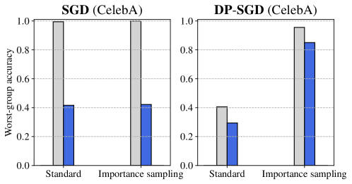
Figure 1: Differential privacy ensures the desired behavior of importance sampling on test data. The train and test accuracy of ResNets on CelebA, evaluated on the worst-performing (“male, blond”) subgroup. Left: Standard SGD has a large generalization gap on this subgroup, and Importance Sampling (IS) has little effect. Right: DP-SGD provably has small generalization gap on all subgroups, and IS improves subgroup performance as intended. See Section 5 for details.

The focus on scalar metrics such as average error, however, misses many theoretically, practically, and socially relevant aspects of model performance. For example, models with small average error often have high error on salient minority subgroups (Buolamwini and Gebru, 2018; Koenecke et al., 2020). In general, ML models are applied to the heterogeneous and long-tailed data distributions of the real world (Van Horn and Perona, 2017). Attempting to summarize their complex behavior with only a single scalar misses many rich and important aspects of learning.

These issues are compounded for modern overparameterized networks, as their nuanced test-time behavior is not reflected at training time. For example, consider the setting of importance sampling: suppose we know that a certain subgroup of inputs is underrepresented in the training data compared to the test distribution (breaking the i.i.d. assumption). For underparameterized models, we can upsample this underrepresented group to account for the distribution shift (see, e.g., Gretton et al., 2009). This approach, however, is known to empirically fail for overparameterized models (Byrd and Lipton, 2019). Because “what you see” (on the training data) is not “what you get” (at test time), we cannot make principled train-time interventions to affect test-time behaviors. This issue extends beyond importance sampling. For example, theoretically principled methods for distributionally robust optimization (e.g. Namkoong and Duchi (2016)) fail for overparameterized deep networks, and require ad-hoc modifications  (Sagawa et al., 2019a).

We develop a theoretical framework which sheds light on these existing issues, and leads to improved practical methods in privacy, fairness, and distributional robustness. The core object in our framework is what we call the “What You See Is What You Get” (WYSIWYG) property. A training procedure with the WYSIWYG property does not exhibit the “pathologies” of standard stochastic gradient descent (SGD): all test-time behaviors will be expressed on the training data as well, and there will be “no surprises” in generalization.

What You See Is What You Get (WYSIWYG) as a Design Principle.

The WYSIWYG property is desirable for two reasons. The first is diagnostic: as there are “no surprises” at test time, all properties of a model at test time are already evident at the training stage. It cannot be the case, for example, that a WYSIWYG model has small disparate impact on the training data, but large disparate impact at test time. The second reason is algorithmic: to mitigate any unwanted test-time behavior, it is sufficient to mitigate this behavior on the training data. This means that algorithm designers can be concerned only with achieving desirable behavior at train time, as the WYSIWYG property guarantees it holds at test time too. In practice, this enables the usage of many theoretically principled algorithms which were developed in the underparameterized regime to also apply in the modern overparameterized (deep learning) setting. For example, we find that interventions such as importance sampling, or algorithms for distributionally robust optimization, which fail without additional regularization, work exactly as intended with WYSIWYG (See Figure 1 for an illustration).

As WYSIWYG is a high-level conceptual property, we have to formalize it to use in computational practice. We do so using the notion of Distributional Generalization (DG), as introduced by Nakkiran and Bansal (2020); Kulynych et al. (2022). If classical generalization ensures that the values of the model’s loss on the training dataset and at test time are close on average Shalev-Shwartz et al. (2010), distributional generalization ensures that values of any other bounded test function—not only loss—are close on training and test time. We say that a model which satisfies an appropriately high level of distributional generalization exhibits the WYSIWYG property.

Achieving DG in Practice.

Our key observation is that distributional generalization is formally implied by differential privacy (DP) Dwork et al. (2006, 2014)). The spirit of this observation is not novel: DP training is known to satisfy much stronger notions of generalization (e.g., robust generalization, see Section 6 for more details), and stability than standard SGD (Dwork et al., 2015a; Cummings et al., 2016; Bassily et al., 2016; Steinke and Zakynthinou, 2020). We show that a similar connection holds for the notion of distributional generalization, and prove (and improve) tight bounds relating DP, stability, and DG. This guarantees the WYSIWYG property for any method that is differentially-private, including DP-SGD on deep neural networks Abadi et al. (2016).

We demonstrate how DG can be a useful design principle in three concrete settings. First, we show that we can mitigate disparate impact of DP training Bagdasaryan et al. (2019); Pujol et al. (2020) by leveraging importance sampling. Second, we study the setting of distributionally robust optimization (e.g., Sagawa et al., 2019a; Hu et al., 2018). We show how ideas from DP can be used to construct heuristic optimizers, which do not formally satisfy DP, yet empirically exhibit DG. Our heuristics lead to competitive results with SOTA algorithms in five datasets in the distributional robustness setting. Third, we show that the heuristic optimizer is also capable of reducing overfitting of adversarial loss in adversarial training Madry et al. (2018); Zhang et al. (2019); Rice et al. (2020).

Our Contributions.

We develop the theoretical connection between Differential Privacy (DP) and Distributional Generalization (DG), and we leverage our theory to improve empirical performance in privacy, fairness, and robustness applications. Theoretically (Sections 2, 3 and 4):

1. We provide tighter bounds than previously reported connecting DP and strong forms of generalization, and show that DP training methods satisfy DG, thus the WYSIWYG property.

2. We introduce DP-IS-SGD, an importance-sampling version of DP-SGD, and show it satisfies DP and DG.

Experimentally (Section 5):

1. We use our framework to shed light on disparate impact: The disparity in accuracy across groups at test time is provably reflected by the accuracy disparity on the train dataset.

2. We use our DP-IS-SGD algorithm to largely mitigate the disparate impact of DP using importance sampling.

3. Based on our theoretical intuitions, we propose a DP-inspired heuristic: addition of gradient noise. We find this empirically achieves competitive and even improved results in several DRO settings, and reduces overfitting of adversarial loss in adversarial training.

Taken together, our results emphasize the central role of the WYSIWYG property in designing machine learning algorithms which avoid the “pathologies” of standard SGD. We also establish DP as a useful tool for achieving WYSIWYG, thus extend its applications further beyond privacy.

2 Theory of “What You See is What You Get” Generalization

We first review the notion of distributional generalization and demonstrate why it captures the WYSIWYG property. Second, we show that strong stability notions imply distributional generalization. Finally, we improve on the known stability guarantees of differential privacy. As a result, we extend the connections between differential privacy, stability, and generalization to distributional generalization, showing that stability and privacy imply the WYSIWYG property.

Notation.

We consider a learning task with a set of examples $\mathbb{X}$ and labels $\mathbb{Y}$. We assume that a source distribution of labeled examples $z~{}\smash{\triangleq}~{}(x,y)\sim\mathcal{D}$ is defined over $\mathbb{D}=\mathbb{X}\times\mathbb{Y}$. Given an i.i.d.-sampled dataset $S\sim\mathcal{D}^{n}$ of size $n$, we use a randomized training algorithm $\mathcal{T}(S)$ that outputs a model’s parameter vector $\theta$ from the set $\Theta$. We denote by $f_{\theta}(x)$ the resulting prediction function.

2.1 Distributional Generalization and WYSIWYG

If on-average generalization Shalev-Shwartz et al. (2010) guarantees closeness only of loss values on train and test data, distributional generalization (DG) also guarantees closeness of values of all test functions $\phi(z;\theta)\in[0,1]$ beyond only loss:

Definition 2.1 (Based on Nakkiran and Bansal (2020)).

An algorithm $\mathcal{T}(S)$ satisfies $\delta$-distributional generalization if for all $\phi:\mathbb{D}\times\Theta\rightarrow[0,1]$,

$$\Big{|}\operatorname*{\mathbb{E}}_{\begin{subarray}{c}S\sim\mathcal{D}^{n}\\ z\sim S\end{subarray}}\phi\big{(}z;\mathcal{T}(S)\big{)}-\operatorname*{\mathbb{E}}_{\begin{subarray}{c}S\sim\mathcal{D}^{n}\\ z\sim\mathcal{D}\end{subarray}}\phi\big{(}z;\mathcal{T}(S)\big{)}\Big{|}\leq\delta.$$ (1)

By the variational characterization of the total-variation (TV) distance (see, e.g., Polyanskiy and Wu, 2014, Chapter 6.3), Equation 1 is equivalent to the bound $d_{\mathsf{TV}}(P_{1},P_{0})\leq\delta,$ where $P_{1}$ and $P_{0}$ are both distributions of $\big{(}z,\mathcal{T}(S)\big{)}$ over the randomness of $S\sim\mathcal{D}^{n}$ and the training algorithm $\mathcal{T}(\cdot)$, with the difference that $z\sim S$ in the case of $P_{1}$ (train), and $z\sim\mathcal{D}$ in the case of $P_{0}$ (test).

It might seem that DG only ensures average closeness of bounded tests on train and test data. This is not, however, the full picture. Consider generalization in terms of a broader class of functions:

Definition 2.2 (Kulynych et al. (2022)).

An algorithm $\mathcal{T}(S)$ satisfies $(\delta,\pi)$-distributional generalization if for a given property function $\pi:\mathbb{D}\times\Theta\rightarrow\mathbb{R}^{k}$ it holds that $d_{\mathsf{TV}}(\pi_{\sharp}P_{1},\pi_{\sharp}P_{0})\leq\delta,$ where $\pi_{\sharp}P$ is the distribution of $\pi(T)$ for $T\sim P$.

Because TV distance is preserved under post-processing, we can see that $\delta$-distributional generalization implies $(\delta,\pi)$-distributional generalization for all property functions. Informally, $\delta$-DG means that for all numeric property functions $\pi(z;\theta)$ of a model, the distributions of the property values are close on the train and test data, on average. This fact captures the high-level idea of the “What You See is What You Get” (WYSIWYG) guarantee. Some example property functions:

• Subgroup loss: $\pi(z;\theta)=\mathbbm{1}\{z\in G\}\cdot\ell(z;\theta)$, for some subgroup $G\subset\mathbb{D}$.

• Counterfactual fairness: $\pi((x,y);\theta)=f_{\theta}(x^{\prime})-f_{\theta}(x)$, where $x^{\prime}$ is a counterfactual version of $x$ had it had a different value of a sensitive attribute Kusner et al. (2017).

• Robustness to corruptions: $\pi(z;\theta)=\ell(A(z);\theta)$, where $A(x)$ is a possibly randomized transformation that distorts the example, e.g., by adding Gaussian noise.

• Adversarial robustness: $\pi(z;\theta)=\ell(A_{\theta}(z);\theta)$, where $A_{\theta}(z)$ is an adversarial example, e.g. generated using the PGD attack Madry et al. (2018).

In the next sections, we show how a training algorithm can provably satisfy DG and therefore provide WYSIWYG guarantees for all properties, including the ones above.

2.2 Distributional Generalization from Stability and Differential Privacy

The connections between privacy, stability, and generalization are well-known. In particular, stability of the learning algorithm—its non-sensitivity to limited changes in the training data—implies generalization Bousquet and Elisseeff (2002); Shalev-Shwartz et al. (2010). In turn, differential privacy implies strong forms of stability, thus ensuring generalization through the chain Privacy $\Rightarrow$ Stability $\Rightarrow$ Generalization Raskhodnikova et al. (2008); Dwork et al. (2015b, a); Wang et al. (2016).

Let us formally define differential privacy:

Definition 2.3 (Differential Privacy Dwork et al. (2006, 2014)).

An algorithm $\mathcal{T}(S)$ is $(\epsilon,\delta)$-differentially private (DP) if for any two neighbouring datasets—differing by one example—$S$, $S^{\prime}$ of size $n$, for any subset $K\subseteq\Theta$ it holds that $\Pr[\mathcal{T}(S)\in K]\leq\exp(\epsilon)\Pr[\mathcal{T}(S^{\prime})\in K]+\delta.$

DP mathematically encodes a notion of plausible deniability of the inclusion of an example in the dataset. However, it can also be thought as a strong form of stability Dwork et al. (2015b). As such, DP implies other notions of stability. We consider the following notion, which has been studied in the literature under multiple names. In the context of privacy, it is equivalent to $(0,\delta)$-differential privacy, and has been called additive differential privacy Geng et al. (2019), and total-variation privacy Barber and Duchi (2014). In the context of learning, it has been called total-variation (TV) stability Bassily et al. (2016). We take this last approach and refer to it as TV stability:

Definition 2.4 (TV Stability).

An algorithm $\mathcal{T}(S)$ is $\delta$-TV stable if for any two neighbouring datasets $S$, $S^{\prime}$ of size $n$, for any subset $T\subseteq\Theta$ it holds that $\Pr[\mathcal{T}(S)\in K]\leq\Pr[\mathcal{T}(S^{\prime})\in K]+\delta.$

It is easy to see that $(\epsilon,\delta)$-DP immediately implies $\delta^{\prime}$-TV stability with:

$$\delta^{\prime}=\exp(\epsilon)-1+\delta.$$ (2)

From Classical to Distributional Generalization.

Similarly to the classical generalization, one way to achieve distributional generalization is through strong stability:

Theorem 2.5.

Suppose that the training algorithm is $\delta$-TV stable. Then, the algorithm satisfies $\delta$-DG.

We refer to Appendix B for the proofs of this and all other formal statements in the rest of the paper.

As DP implies TV-stability, by Theorem 2.5 we have that DP also implies DG. We show that DP algorithms enjoy a significantly stronger stability guarantee than previously known, which means that the DG guarantee that one obtains from DP is also stronger.

Proposition 2.6.

An algorithm which is $(\epsilon,\delta)$-DP is also $\delta^{\prime}$-TV stable with:

$$\delta^{\prime}=\frac{\exp(\epsilon)-1+2\delta}{\exp(\epsilon)+1}.$$

Figure 2: DG bound from $(\epsilon,0)$-DP.

In Section A.2, we discuss the relationship of this result to other works in the literature on information-theoretic generalization. In particular, to Steinke and Zakynthinou (2020) whose results can also be used to relate DP and DG. Figure 2 shows that the known bounds quickly become vacuous unlike the bound in Proposition 2.6. In fact, we show that our bound is tight in Appendix B.

Stronger Distributional Generalization Guarantees. Although DG immediately implies generalization for all bounded properties, it is possible to obtain tighter bounds from TV stability. For example, directly applying DG to the subgroup loss property yields a bound that decays with the size of the subgroup: accuracy on very small subgroups is not guaranteed to generalize well. In Section C.1 we show that TV stability implies “subgroup DG”, which guarantees that the accuracy on even small subgroups generalizes well in expectation. As another example, in Section C.2 we show that TV stability also ensures generalization of calibration properties of the learning algorithm.

3 Example Applications

To demonstrate that WYSIWYG is a useful property in algorithm design, in the remainder of this paper we use it to construct simple and high-performing algorithms for three example applications: mitigation of disparate impact of DP, ensuring group-distributional robustness, and mitigation of robust overfitting in adversarial training.

Mitigating Disparate Impact of DP.

First, we consider applications in which learning presents privacy concerns, e.g., in the case that the training data contains sensitive information. Using training procedures that satisfy DP is a standard way to guarantee privacy in such settings. Training with DP, however, is known to incur disparate impact on the model accuracy: some subgroups of inputs can have worse test accuracy than others. For example, Bagdasaryan et al. (2019) show that using DP-SGD—a standard algorithm for satisfying DP Abadi et al. (2016)—in place of regular SGD causes a significant accuracy drop on “darker skin” faces in models trained on the CelebA dataset of celebrity faces Liu et al. (2015), but a less severe drop on “lighter skin” faces. Our goal is to mitigate such disparate impact. This issue—a quality-of-service harm Madaio et al. (2020)—is but one of many possible harms due to ML systems. We do not aim to mitigate any other broad fairness-related issues, nor claim this is possible within our framework.

Formally, we assume the data distribution $\mathcal{D}$ is a mixture of $m$ groups indexed by set $\mathcal{G}=\{1,\ldots,m\}$, such that $\mathcal{D}=\sum_{i=1}^{m}q_{i}\mathcal{D}_{i}$. The vector $(q_{i},\ldots,q_{m})\in[0,1]^{m}$ represents the group probabilities, with $\sum_{i=1}^{m}q_{i}=1$. For given parameters $(\epsilon,\delta)$, we want to learn a model $\theta$ that simultaneously satisfies $(\epsilon,\delta)$-DP, has high overall accuracy, and incurs small loss disparity:

$$\max_{g,g^{\prime}\in\mathcal{G}}\left|\operatorname*{\mathbb{E}}_{z\sim\mathcal{D}_{g}}[\ell(z;\theta)]-\operatorname*{\mathbb{E}}_{z\sim\mathcal{D}_{g^{\prime}}}[\ell(z;\theta)]\right|.$$ (3)

Group-Distributional Robustness.

Next, we consider a setting of group-distributionally robust optimization (e.g., Sagawa et al., 2019a; Hu et al., 2018). If in the standard learning approach we want to train a model that minimizes average loss, in this setting, we want to minimize the worst-case (highest) group loss. This objective can be used to mitigate fairness concerns such as those discussed previously, as well as to avoid learning spurious correlations Sagawa et al. (2019a).

Formally, we want to learn a model $\theta$ that minimizes the worst-case group loss:

$$\max_{g\in\mathcal{G}}\operatorname*{\mathbb{E}}_{z\sim\mathcal{D}_{g}}\left[\ell(z;\theta)\right].$$ (4)

Unlike the previous application, in this setting, we do not require privacy of the training data. We use training with DP as a tool to ensure the generalization of the worst-case group loss.

Mitigating Robust Overfitting.

Finally, we consider the setting of robustness to test-time adversarial examples through adversarial training Goodfellow et al. (2014). A common way to train robust models in this sense in image domains is to minimize robust (adversarial) loss Madry et al. (2018):

$$\operatorname*{\mathbb{E}}_{(x,y)\sim\mathcal{D}}\left[\max_{\|x-x_{\mathsf{adv}}\|_{p}\leq\gamma}\ell((x_{\mathsf{adv}},y);\theta)\right],$$ (5)

where $\gamma>0$ is a small constant. Rice et al. (2020) observed that adversarially trained models exhibit “robust overfitting”: higher generalization gap of robust loss than that of the regular loss. In this application, we similarly aim to use a relaxed version of training with DP as a tool to ensure generalization of robust loss, thus mitigate robust overfitting.

4 Algorithms which Distributionally Generalize

In this section, we construct algorithms for the applications in Section 3. Our approach follows the blueprint: First, we apply a principled algorithmic intervention that ensures desired behavior on the training data (e.g., importance sampling). Second, we modify the resulting algorithm to additionally ensure DG, which guarantees that the desired behavior generalizes to test time.

4.1 DP Training with Importance Sampling

Our first algorithm, DP-IS-SGD (Algorithm 1), is a version of DP-SGD Abadi et al. (2016) which performs importance sampling. DP-IS-SGD is designed to mitigate disparate impact while retaining DP guarantees. The standard DP-SGD samples data batches using uniform Poisson subsampling: Each example in the training set is chosen into the batch according to the outcome of a Bernoulli trial with probability $\bar{p}\in[0,1]$. To correct for unequal representation and the resulting disparate impact, we use non-uniform Poisson subsampling: Each example $z\in S$ has a possibly different probability $p(z)$ of being selected into the batch, where $p(z)$ does not depend on the dataset $S$ otherwise, and is bounded: $0\leq p(z)\leq p^{*}\leq 1$. We denote this subsampling procedure as $\mathsf{Sample}_{p(\cdot)}(S)$.

We assume that we know to which group any $z=(x,y)$ belongs, denoted as $g(z)$, e.g., the group is one of the features in $x$. We choose $p(z)$ to satisfy two properties. First, to increase the sampling probability for examples in minority groups: $p(z)\propto\nicefrac{{1}}{{q_{g(z)}}}$. Second, to keep the average batch size equal to $\bar{p}\cdot n$ as in standard DP-SGD. In the rest of the paper, we assume that the group probabilities $(q_{1},\ldots,q_{m})$ are known, but it is possible to estimate them in a private way using standard methods Nelson and Reuben (2020). We present DP-IS-SGD in Algorithm 1, along with its differences to the standard DP-SGD.

Algorithm 1 DP-IS-SGD (DP Importance Sampling SGD)

Dataset $S$, loss $\ell(z;\theta)$, initial parameters $\theta_{0}$, learning rate $\eta$, maximal gradient norm $C$, noise parameter $\sigma$, number of epochs $T$, sampling rate $\bar{p}$, $\mathchoice{\hbox{\pagecolor{blue!20}$\displaystyle\text{group probabilities }(q_{1},\ldots,q_{m})$}}{\hbox{\pagecolor{blue!20}$\textstyle\text{group probabilities }(q_{1},\ldots,q_{m})$}}{\hbox{\pagecolor{blue!20}$\scriptstyle\text{group probabilities }(q_{1},\ldots,q_{m})$}}{\hbox{\pagecolor{blue!20}$\scriptscriptstyle\text{group probabilities }(q_{1},\ldots,q_{m})$}}.$

for $t=1,\ldots,T$ do

     Sample batch $S_{t}\leftarrow\mathchoice{\hbox{\pagecolor{blue!20}$\displaystyle\smash{\mathsf{Sample}_{p(\cdot)}}(S)\text{, with sampling probabilities }p(z)~{}\smash{\triangleq}~{}\nicefrac{{\bar{p}}}{{m\cdot q_{g(z)}}}$}}{\hbox{\pagecolor{blue!20}$\textstyle\smash{\mathsf{Sample}_{p(\cdot)}}(S)\text{, with sampling probabilities }p(z)~{}\smash{\triangleq}~{}\nicefrac{{\bar{p}}}{{m\cdot q_{g(z)}}}$}}{\hbox{\pagecolor{blue!20}$\scriptstyle\smash{\mathsf{Sample}_{p(\cdot)}}(S)\text{, with sampling probabilities }p(z)~{}\smash{\triangleq}~{}\nicefrac{{\bar{p}}}{{m\cdot q_{g(z)}}}$}}{\hbox{\pagecolor{blue!20}$\scriptscriptstyle\smash{\mathsf{Sample}_{p(\cdot)}}(S)\text{, with sampling probabilities }p(z)~{}\smash{\triangleq}~{}\nicefrac{{\bar{p}}}{{m\cdot q_{g(z)}}}$}}$

     $\tilde{g}_{t}\leftarrow\frac{1}{|S_{t}|}\sum_{z\in S_{t}}\underbrace{\nicefrac{{1}}{{\max\{1,~{}C^{-1}\cdot\|\nabla_{\theta}\ell(z;\theta)\|_{2}\}}}}_{\text{Gradient clipping}}\cdot\nabla_{\theta}\ell(z;\theta)+\underbrace{\sigma C\cdot\mathcal{N}(0,I)}_{\text{Gradient noise}}$

     $\theta_{t}\leftarrow\theta_{t-1}+\eta\cdot\tilde{g}_{t}$

The highlighted parts indicate the differences with respect to DP-SGD. We obtain DP-SGD as a special case when we have a single group with $q=1$ (implying $p(z)=\bar{p}$).

DP Properties of DP-IS-SGD.

Uniform Poisson subsampling is well-known to amplify the privacy guarantees of an algorithm Chaudhuri and Mishra (2006); Li et al. (2012). For example, Li et al. (2012) show that if an algorithm $\mathcal{T}(S)$ satisfies $(\epsilon,\delta)$-DP, then $\mathcal{T}\circ\smash{\mathsf{Sample}_{\bar{p}}}(S)$ provides approximately $(O(\bar{p}\epsilon),\bar{p}\delta)$-DP for small values of $\epsilon$. We show in Appendix B that non-uniform Poisson subsampling provides the same amplification guarantee with $\bar{p}=p^{*}$, where $p^{*}$ is the maximum value of $p(\cdot)$.

As this guarantee is independent of the internal workings of $\mathcal{T}(S)$, it is loose. For DP-SGD, one way of computing tight privacy guarantees of subsampling is using the notion of Gaussian differential privacy (GDP) Dong et al. (2019). GDP is parameterized by a single parameter $\mu$. If an algorithm $\mathcal{T}(S)$ satisfies $\mu$-GDP, one can efficiently compute a set of $(\epsilon,\delta)$-DP guarantees also satisfied by $\mathcal{T}(S)$ Dong et al. (2019). We show that we can use any GDP-based mechanism for computing the privacy guarantee of DP-SGD to obtain the privacy guarantees of DP-IS-SGD in a black-box manner:

Proposition 4.1.

Let us denote by $\mu(\bar{p},\sigma,C,T)$ (see Algorithm 1) a function that returns a $\mu$-GDP guarantee of DP-SGD. Then, DP-IS-SGD satisfies a GDP guarantee $\mu(p^{*},\sigma,C,T)$.

4.2 Gaussian Gradient Noise

We showed that DP-IS-SGD enjoys theoretical guarantees for both DP and DG. DP models, however, often have lower test accuracy compared to standard training Chaudhuri et al. (2011). This can be an unnecessary disadvantage in settings where privacy is not required, such as in our robustness applications. Thus, we explore training algorithms which are inspired by our theory yet do not come with generic theoretical guarantees of DG.

Note that DP-SGD uses gradient clipping and noise (see Algorithm 1). Individually, these are used as regularization methods for improving stability and generalization Hardt et al. (2016); Neelakantan et al. (2015). Following this, we relax DP-IS-SGD to only use gradient noise. This sacrifices privacy guarantees in exchange for practical performance. Specifically, we apply gradient noise to three standard algorithms for achieving group-distributional robustness: importance sampling (IS-SGD), importance weighting (IW-SGD) Gretton et al. (2009), and gDRO Sagawa et al. (2019a). This results in the following variations: IS-SGD-n, IW-SGD-n, gDRO-n, respectively. Similarly, we apply gradient noise to standard PGD adversarial training Madry et al. (2018). See Appendix D for details.

5 Experiments

We empirically study the distributional generalization in real-world applications. The code for the experiments is available at https://github.com/yangarbiter/dp-dg.

Datasets.

We use the following datasets with group annotations: CelebA (Liu et al., 2015), UTKFace (Zhang et al., 2017), iNaturalist2017 (iNat) Horn et al. (2018), CivilComments Borkan et al. (2019), MultiNLI Williams et al. (2018); Sagawa et al. (2019a), and ADULT Kohavi et al. (1996). For every dataset, each example belongs to one group (e.g., CelebA) or multiple groups (e.g., CivilComments). For example, in the CelebA dataset, there are four groups: “blond male”, “male with other hair color”, “blond female”, and “female with other hair color”. Additionally, we use the CIFAR-10 Krizhevsky et al. (2009) dataset for the adversarial-overfitting application. We present more details on the datasets, their groups, and used model architectures in Appendix E.

5.1 Enforcing DG in Practice

We empirically confirm that a training procedure with DP guarantees also has a bounded DG gap.

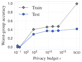
Figure 3: Privacy induces DG. Train/test worst-case group accuracies as a function of privacy parameter $\epsilon$ of DP-SGD on CelebA (x axis). Increasing privacy reduces the generalization gap.

In practice, it is not possible to compute the exact DG gap. As a proxy in applications which concern subgroup performance in this section, and Sections 5.2 and 5.3, we use the difference between train-time and test-time worst-group accuracy. This (a) follows the empirical approach by Nakkiran and Bansal (2020) which proposes to estimate the gap in Equation 1 using a finite set of test functions, and (b) measures the aspect of distributional generalization that is relevant to our applications. We provide more details on this choice of the proxy measure in Section E.2.

We train a model on CelebA using DP-SGD for varying levels of $\epsilon$. Figure 3 shows that the gap between training and testing worst-group accuracy increases as the level of privacy decreases, which is consistent with our theoretical bounds. In Section E.3 we also explore how regularization methods which do not necessarily formally imply DG, can empirically improve DG.

5.2 Disparate Impact of Differentially Private Models

We evaluate DP-IS-SGD (Algorithm 1), and demonstrate that it can mitigate the disparate impact in realistic settings where both privacy and fairness are required.

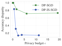
(a) Accuracy disparity (lower is better)

(b) Worst-group accuracy (higher is better)

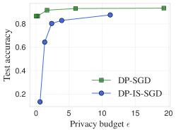
(c) Test accuracy (higher is better)

Figure 4: Importance Sampling Improves Disparate Impact of DP-SGD. The accuracy disparity of the models trained with DP-SGD and DP-IS-SGD on CelebA. Adding importance sampling (IS) improves disparate impact at most privacy budgets in this setting. We set $\delta=\nicefrac{{1}}{{2n}}$, where $n$ is the number of training examples. We use GDP accountant to compute the privacy budget $\varepsilon$.

Figure 4 shows the accuracy disparity, test accuracy, and worst-case group accuracy, computed as in Equation 3, as a function of the privacy budget $\epsilon$. The models are trained with DP-SGD and DP-IS-SGD. When comparing DP-SGD and DP-IS-SGD with the same or similar $\epsilon$, we observe that DP-IS-SGD achieves lower disparity on all datasets. However, this comes with a drop in average accuracy. On CelebA, with $\epsilon\in[2,12]$, DP-IS-SGD has around 8 p.p. lower test accuracy than DP-SGD. At the same time, the disparity drop ranges from 40 p.p. to 60 p.p., which is significantly higher than the accuracy drop. We observe similar results on UTKFace. On iNat, however, although DP-IS-SGD decreases disparity, the overall test accuracy suffers a significant hit. This is likely because the minority subgroup is very small, which results in high maximum sampling probability $p^{*}$, thus deteriorating the privacy guarantee. Details for UTKFace and iNat are in Section E.4.

In summary, we find that DP-IS-SGD can achieve lower disparity at the same privacy budget compared to standard DP-SGD, with mild impact on test accuracy.

Comparison to DP-SGD-F Xu et al. (2021).

DP-SGD-F is a variant of DP-SGD which dynamically adapts gradient-clipping bounds for different groups to reduce the disparate impact. We did not manage to achieve good overall performance of DP-SGD-F on the datasets above. In Section E.4, we compare it to DP-IS-SGD on the ADULT dataset (used by Xu et al. (2021)), finding that DP-IS-SGD obtains lower disparity for the same privacy level, yet also lower overall accuracy.

5.3 Group-Distributionally Robust Optimization

We investigate whether our proposed versions of standard algorithms with Gaussian gradient noise (Section 4.2) can improve group-distributional robustness. To do so, we evaluate empirical DG using worst-group accuracy as a proxy for DG gap as in Section 5.1, following the evaluation criteria in prior work (Sagawa et al., 2019a; Idrissi et al., 2022). State-of-the-art (SOTA) methods apply $\ell_{2}$ regularization and early-stopping to achieve the best performance. We compare three baselines with $\ell_{2}$ regularization, IS-SGD-$\ell_{2}$, IW-SGD-$\ell_{2}$, and gDRO-$\ell_{2}$ to our noisy-gradient variations as well as DP-IS-SGD. We use the validation set to select the best-performing regularization parameter and epoch (for early stopping) for each method. See Section E.5 for details on the experimental setup.

Table 1 shows the worst-group accuracy of each algorithm on five datasets. When comparing IS-SGD, IW-SGD, and gDRO with their noisy counterparts, we observe that the noisy versions in general have similar or slightly better performance compared to non-noisy counterparts. For instance, IS-SGD-n improves the SOTA results on CivilComments dataset. This showcases that in terms of learning distributionally robust models, noisy gradient can be a more effective regularizer than the currently standard $\ell_{2}$ regularizer. We also find that DP-IS-SGD improves on baseline methods or even achieves SOTA-competetitive performance on several datasets. For instance, on CelebA and MNLI, DP-IS-SGD achieves better performance than IS-SGD-$\ell_{2}$. This is surprising, as DP tends to deteriorate performance. This suggests that distributional robustness and privacy are not incompatible goals. Moreover, DP can be a useful tool even when privacy is not required.

Table 1: Our noisy-gradient algorithms produce competitive results compared to counterparts with $\ell_{2}$ regularization. The table shows the worst-group accuracy of each algorithm. Baselines are in the top rows; our algorithms are in the bottom. For gDRO-$\ell_{2}$-SOTA, we show avg. $\pm$ std. over five runs from Idrissi et al. (2022). For CelebA, we show avg. $\pm$ std. over three random splits.

	CelebA	UTKFace	iNat.	Civil.	MNLI
SGD-$\ell_{2}$	73.0 $\pm$ 2.2	86.3	41.8	57.4	67.9
IS-SGD-$\ell_{2}$	82.4 $\pm$ 0.5	85.8	70.6	64.3	70.4
IW-SGD-$\ell_{2}$	89.0 $\pm$ 0.9	86.5	67.6	65.7	68.1
gDRO-$\ell_{2}$	84.5 $\pm$ 0.8	85.2	67.3	67.3	75.9
gDRO-$\ell_{2}$-SOTA	86.9 $\pm$ 0.5	—	—	69.9 $\pm$ 0.5	78.0 $\pm$ 0.3
DP-IS-SGD	86.0 $\pm$ 0.8	82.5	51.4	70.4	72.3
IS-SGD-n	84.9 $\pm$ 1.0	85.5	71.0	71.9	70.8
IW-SGD-n	88.5 $\pm$ 0.4	88.5	70.9	69.9	69.7
gDRO-n	83.3 $\pm$ 0.5	87.5	56.4	71.3	78.0

5.4 Mitigating Robust Overfitting

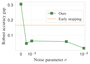
(a) Gen. gap of robust accuracy (lower is better)

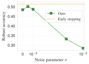
(b) Robust accuracy (higher is better)

Figure 5: Noisy gradient reduces overfitting in adversarial training. We show the generalization gap of robust accuracy (left), and test-time robust accuracy (right) of adversarially trained models with different levels of noise magnitude. The dash orange lines represent the performance of adversarial training with early stopping. The model trained without noise exhibits “robust overfitting” of about 30 p.p. Gradient noise reduces the generalization gap by more than 3$\times$ for all values of the noise parameter at a cost of decreased robust accuracy as the noise gets larger.

As in the previous section, we expect that a modification of a standard projected gradient descent (PGD) method for adversarial training Madry et al. (2018) with added Gaussian gradient noise (Section 4.2) improves the generalization behavior of adversarial training.

To verify this, we adversarially train models on the CIFAR-10 dataset with varying levels of the noise magnitude. We provide more details on the setup in Section E.6. Figure 5 shows that in standard adversarial training without noise the gap between robust training accuracy and robust test accuracy is large at approximately 30 p.p., which is consistent with the prior observations of Rice et al. (2020). By injecting noise into the gradient, our proposed approach decreases the generalization gap of robust accuracy by more than 3$\times$ to less than 10 p.p. Surprisingly, in our experiments, training with gradient noise achieves both a small adversarial accuracy gap and better adversarial test accuracy compared to standard adversarial training, when using a small noise magnitude ($\sigma=5\times 10^{-4}$). In terms of resulting robust accuracy, the method’s performance is comparable to early stopping, identified as the most effective way to prevent robust overfitting by Rice et al. (2020). These experimental results demonstrate how WYSIWYG can be a useful design principle in practice.

6 Related Work

DP and Strong Generalization. DP is known to imply a stronger than standard notion of generalization, called robust generalization  (Cummings et al., 2016; Bassily et al., 2016). Robust generalization can be thought as a high-probability counterpart of DG: generalization holds with high probability over the train dataset, not only on average over datasets. We focus on our notion of DG for both conceptual and theoretical simplicity. A more comprehensive discussion of relations to robust generalization is in Appendix A.1. It can also be useful to consider intermediary definitions, varying in strength from DG to robust generalization. In Appendix C, we introduce such an notion (“strong DG”) and show its connections to DP. Other than robust generalization, our connections in Section 2 can also be derived from weaker generalization bounds that rely on information-theoretic measures Steinke and Zakynthinou (2020). We detail this in Section A.2.

Disparate Impact of DP. Bagdasaryan et al. (2019); Pujol et al. (2020) have shown that ensuring DP in algorithmic systems can cause error disparity across population groups. Xu et al. (2021) proposed a variant of DP-SGD for reducing disparate impact. We compare our method to DP-SGD-F in Section E.4. In another line of related work, Sanyal et al. (2022); Cummings et al. (2019) show fundamental trade-offs between model’s loss and DP training. As our theoretical results concern generalization, not loss per se, our results do not contradict these theoretical trade-offs. We discuss the relationship in detail in Section A.3.

Group-Distributional Robustness. Group-distributional robustness aims to improve the worst-case group performance. Existing approaches include using worst-case group loss (Mohri et al., 2019; Sagawa et al., 2019a; Zhang et al., 2020), balancing majority and minority groups by reweighting or subsampling (Byrd and Lipton, 2019; Sagawa et al., 2019b; Idrissi et al., 2022), leveraging generative models (Goel et al., 2020), and applying various regularization techniques (Sagawa et al., 2019a; Cao et al., 2019). Although some work (Sagawa et al., 2019a; Cao et al., 2019) discusses the importance of regularization in distributional robustness, they have not explored potential reasons for this (e.g. via the connection to generalization). Another line of work studies how to improve group performance without group annotations (Duchi et al., 2021; Liu et al., 2021; Creager et al., 2021), which is a different setting from ours as we assume the group annotations are known.

Robust Overfitting. Rice et al. (2020); Yu et al. (2022) have shown that adversarially trained models tend to overfit in terms of robust loss. Rice et al. (2020) proposed to use regularization to mitigate overfitting, but the noisy gradient has not been explored for this. We showed that the WYSIWYG framework can serve as an alternative direction for mitigating and explaining this issue.

7 Conclusions and Future Work

We argue that a “What You See is What You Get” property, which we formalize through the notion of distributional generalization (DG), can be desirable for learning algorithms, as it enables principled algorithm design in settings including deep learning. We show that this property is possible to achieve with DP training. This enables us to leverage advances in DP to enforce DG in many applications.

We propose enforcing DG as a general design principle, and we use it to construct simple yet effective algorithms in three settings. In certain fairness settings, we largely mitigate the disparate impact of differential privacy by using importance sampling and enforcing DG in our new algorithm DP-IS-SGD. In our analysis, however, the privacy and DG guarantees of DP-IS-SGD deteriorate in the presence of very small groups. Future work could explore individual-level accounting Feldman and Zrnic (2021) for a tighter analysis. In certain worst-case generalization settings, inspired by DP-SGD, we propose using a noisy-gradient regularizer. Compared to SOTA algorithms in DRO, noisy gradient achieves competitive results across many standard benchmarks. In certain adversarial-robustness settings, our proposed noisy-gradient regularizer significantly reduces robust overfitting. An interesting direction for future work would be to explore its effectiveness in large-scale settings, e.g., ImageNet (Croce and Hein, 2022). We hope future work can explore extending this design principle to ensure generalization of other properties, such as calibration and counterfactual fairness.

Acknowledgements

We thank Kamalika Chaudhuri, Benjamin L. Edelman, Saurabh Garg, Gautam Kamath, Maksym Andriushchenko, and Cassidy Laidlaw for useful feedback on an early draft. BK acknowledges support from the Swiss National Science Foundation with grant 200021-188824. Yao-Yuan Yang thanks NSF under CNS 1804829 and ARO MURI W911NF2110317 for the research support. Yaodong Yu acknowledges support from the joint Simons Foundation-NSF DMS grant #2031899. PN is grateful for support of the NSF and the Simons Foundation for the Collaboration on the Theoretical Foundations of Deep Learning through awards DMS-2031883 and #814639.

Checklist

1. For all authors…

   1. Do the main claims made in the abstract and introduction accurately reflect the paper’s contributions and scope? [Yes]

   2. Did you describe the limitations of your work? [Yes] We address the limitations where appropriate, e.g., high-level limitations in Section 3, and the fact that some methods we use in the empirical evaluations deviate from theory in Sections 4 and 5.

   3. Did you discuss any potential negative societal impacts of your work? [Yes] In Section 3 we caution against using WYSIWYG for fairness-washing Bietti [2020] through technical solutionism. Other than this, our potential negative societal impacts are the same as with any other academic work which aims to improve the performance of deep learning: we risk improving performance of deep learning in downstream applications that are harmful, e.g., privacy-invasive, or violating other civil liberties. It is beyond the scope of our work to discuss such broad issues.

   4. Have you read the ethics review guidelines and ensured that your paper conforms to them? [Yes]

2. If you are including theoretical results…

   1. Did you state the full set of assumptions of all theoretical results? [Yes]

   2. Did you include complete proofs of all theoretical results? [Yes] See Appendix B.

3. If you ran experiments…

   1. Did you include the code, data, and instructions needed to reproduce the main experimental results (either in the supplemental material or as a URL)? [Yes] We included the experiment code as supplemental material.

   2. Did you specify all the training details (e.g., data splits, hyperparameters, how they were chosen)? [Yes] See Appendix E.

   3. Did you report error bars (e.g., with respect to the random seed after running experiments multiple times)? [Yes] For experimental settings in which it was feasible for us to repeat experiments multiple times, we reported the standard errors (Table 1).

   4. Did you include the total amount of compute and the type of resources used (e.g., type of GPUs, internal cluster, or cloud provider)? [Yes] See Section E.1.

4. If you are using existing assets (e.g., code, data, models) or curating/releasing new assets…

   1. If your work uses existing assets, did you cite the creators? [Yes] See Section E.1.

   2. Did you mention the license of the assets? [Yes] See Section E.1.

   3. Did you include any new assets either in the supplemental material or as a URL? [N/A]

   4. Did you discuss whether and how consent was obtained from people whose data you’re using/curating? [Yes] See Section E.1.

   5. Did you discuss whether the data you are using/curating contains personally identifiable information or offensive content? [Yes] See Section E.1.

5. If you used crowdsourcing or conducted research with human subjects…

   1. Did you include the full text of instructions given to participants and screenshots, if applicable? [N/A]

   2. Did you describe any potential participant risks, with links to Institutional Review Board (IRB) approvals, if applicable? [N/A]

   3. Did you include the estimated hourly wage paid to participants and the total amount spent on participant compensation? [N/A]

Appendix A Related Work Details

A.1 Differential Privacy and Robust Generalization

DP is known to imply a stronger notion of generalization, called robust generalization, which is a “tail bound” version of DG [Dwork et al., 2015a, Cummings et al., 2016, Bassily et al., 2016]. The original motivations for robust generalization are slightly different, but in our notation, a training procedure $\mathcal{T}$ is said to satisfy $(\gamma,\eta)$-Robust Generalization if and only if for any test $\phi:\mathbb{D}\times\Theta\rightarrow[0,1]$, we have

$$\Pr_{\begin{subarray}{c}S\sim\mathcal{D}^{n},\mathcal{T}\end{subarray}}\left(\big{|}\operatorname*{\mathbb{E}}_{z\sim S}\phi\big{(}z;\mathcal{T}(S)\big{)}-\operatorname*{\mathbb{E}}_{z\sim\mathcal{D}}\phi\big{(}z;\mathcal{T}(S)\big{)}\big{|}>\gamma\right)\leq\eta.$$

Comparing this to the definition of DG (Definition 2.1), it is immediatelinecolor=red,backgroundcolor=red!25,bordercolor=red]Can you elaborate? –BK that any procedure that satisfies $(\gamma,\eta)$-Robust Generalization, also satisfies $(\gamma+\eta)$-DG. Any training method satisfying $(\epsilon,\delta)$-DP also satisfies $(\mathcal{O}(\epsilon),\mathcal{O}(\delta))$-robust generalization, as long as the sample size $n$ is of size $\Omega(\log(1/\delta)/\epsilon^{2})$ [Bassily et al., 2016, Theorem 7.2], therefore it satisfies $\mathcal{O}(\epsilon+\delta)$-DG by the previous implication. Thus, it is possible to recover the result that DP implies DG as a consequence of these previous works, although with looser bounds.

The difference between Distributional Generalization and Robust Generalization is that DG considers all quantities in expectation, while robust generalization considers tail bounds with respect to the train dataset. We focus on DG for two reasons: First, we believe DG is conceptually simpler, as it can be seen as simply the TV distance between two natural distributions, and does not involve additional parameters. This simplicity is conceptually useful to the algorithm designer, but also enables us to prove simpler tight theoretical bounds that are independent of sample size. Second, it is often possible to lift results about DG to the stronger setting of robust generalization, with additional bookkeeping. Thus, we focus on DG in this paper, with the understanding that stronger guarantees can be obtained for these methods if desired.

A.2 Information-Theoretic Generalization Bounds

Other than robust generalization, it is also possible to obtain bounds on generalization of arbitrary test (loss) functions using information-theoretic measures Xu and Raginsky [2017], Russo and Zou [2019], Steinke and Zakynthinou [2020]. Recently, Steinke and Zakynthinou showed that one such information-theoretic measure—conditional mutual information (CMI) between training algorithm outputs and the training dataset—is bounded if the training algorithm is DP or TV stable. Thus, we could relate stability and DG as in Section 2.2 using CMI as an intermediate tool.

In particular, Steinke and Zakynthinou show that for a given $\phi:\mathbb{D}\times\Theta\rightarrow[0,1]$:

$$\Big{|}\operatorname*{\mathbb{E}}_{\begin{subarray}{c}S\sim\mathcal{D}^{n}\\ z\sim S\end{subarray}}\phi\big{(}z;\mathcal{T}(S)\big{)}-\operatorname*{\mathbb{E}}_{\begin{subarray}{c}S\sim\mathcal{D}^{n}\\ z\sim\mathcal{D}\end{subarray}}\phi\big{(}z;\mathcal{T}(S)\big{)}\Big{|}\leq\sqrt{\frac{2}{n}\cdot\mathrm{CMI}_{\mathcal{D}}(\mathcal{T})},$$ (6)

where $\mathrm{CMI_{\mathcal{D}}}(\mathcal{T})$ is the conditional mutual information of the training algorithm with respect to the data distribution. If the training algorithm satisfies $(\epsilon,0)$-DP, they also show that $\mathrm{CMI_{\mathcal{D}}}(\mathcal{T})\leq\frac{n}{2}\epsilon^{2}$, where $n$ is the dataset size. Plugging this into Equation 6, we can see that the generalization upper bound (right-hand side) is $\epsilon$. This is significantly looser than our bound in Section 2.2, as illustrated in Figure 2.

A recent line of work on information-theoretic bounds explores sharper generalization bounds using individual-level measures Bu et al. [2020a], Haghifam et al. [2020]. Analogously, as a direction for future work, it could also be possible to obtain tighter bounds on DG using per-instance notions of stability Wang [2017], Feldman and Zrnic [2021].

A.3 Tension between Differential Privacy and Algorithmic Fairness

Beyond empirical observations that training with DP results in disparate impact on performance across subgroups Bagdasaryan et al. [2019], Pujol et al. [2020], Cummings et al. [2019] and, more recently, Sanyal et al. [2022] theoretically analyze the inherent tensions between DP and algorithmic fairness.

It might appear that this trade-off contradicts our results in which we claim that using DP or similar noise-adding algorithms with additional train-time interventions can reduce disparate impact. However, Cummings et al. [2019] and Pujol et al. [2020] discuss the relationship between privacy and disparate performance (accuracy or false-positive/false-negative rates), whereas we discuss the relationship between privacy and generalization. Even if a DP model has to incur at least a certain error on small subgroups on average [Sanyal et al., 2022, Lemma 1], this error is guaranteed to be similar at train time and test time (from our theoretical results in Section 2.2).

In terms of empirical results, the lower bound on subgroup error in Lemma 1 from Sanyal et al. [2022] vanishes for subgroups of size greater than 100 even for small values of epsilon (e.g., 0.1). The subgroups and values of epsilon in our experiments in Section 5 are all larger than this, thus in our regime we can achieve meaningful subgroup performance using the DP-IS-SGD algorithm despite the fundamental trade-off.

Appendix B Proofs Omitted in the Main Body

B.1 TV-Stability implies Distributional Generalization

Proof of Theorem 2.5.

First, observe that the following distributions are equivalent as the dataset is an i.i.d. sample:

$$\Pr_{\begin{subarray}{c}S\sim\mathcal{D}^{n}\\ z\sim S\end{subarray}}[\phi\big{(}z;\mathcal{T}(S)\big{)}] \equiv\Pr_{\begin{subarray}{c}S\sim\mathcal{D}^{n-1}\\ z\sim\mathcal{D}\end{subarray}}[\phi\big{(}z;\mathcal{T}({S\cup\{z\}})\big{)}],$$ (7)

$$\Pr_{\begin{subarray}{c}S\sim\mathcal{D}^{n}\\ z\sim\mathcal{D}\end{subarray}}[\phi\big{(}z;\mathcal{T}(S)\big{)}] \equiv\Pr_{\begin{subarray}{c}S\sim\mathcal{D}^{n-1}\\ z\sim\mathcal{D}\\ z^{\prime}\sim\mathcal{D}\end{subarray}}[\phi\big{(}z^{\prime};\mathcal{T}({S\cup\{z\}})\big{)}].$$

It is thus sufficient to analyze the equivalent distributions instead. By the post-processing property of differential privacy, for any dataset $S\in\mathbb{D}^{n-1}$, any two examples $z,z^{\prime}\in\mathbb{D}$, and any set $K\subseteq\{0,1\}$:

$$\Pr[\phi\big{(}z;\mathcal{T}({S\cup\{z\}})\big{)}\in K]\leq\Pr[\phi\big{(}z;\mathcal{T}({S\cup\{z^{\prime}\}})\big{)}\in K]+\delta,$$

as datasets $S\cup\{z\}$ and $S\cup\{z^{\prime}\}$ are neighbouring. Taking the expectation of both sides over $z,z^{\prime}\sim\mathcal{D}$ and $S\sim\mathcal{D}^{n-1}$, we get:

$$\Pr_{\begin{subarray}{c}S\sim\mathcal{D}^{n-1}\\ z\sim\mathcal{D}\end{subarray}}[\phi\big{(}z;\mathcal{T}({S\cup\{z\}})\big{)}\in K] \leq\Pr_{\begin{subarray}{c}S\sim\mathcal{D}^{n-1}\\ z\sim\mathcal{D}\\ z^{\prime}\sim\mathcal{D}\end{subarray}}[\phi\big{(}z;\mathcal{T}({S\cup\{z^{\prime}\}})\big{)}\in K]+\delta$$ (8)

$$=\Pr_{\begin{subarray}{c}S\sim\mathcal{D}^{n-1}\\ z\sim\mathcal{D}\\ z^{\prime}\sim\mathcal{D}\end{subarray}}[\phi\big{(}z^{\prime},\mathcal{T}({S\cup\{z\}})\big{)}\in K]+\delta,$$

where the last equality is simply renaming of the variables for convenience. Note that analogously we also can obtain a symmetric bound:

$$\Pr_{\begin{subarray}{c}S\sim\mathcal{D}^{n-1}\\ z\sim\mathcal{D}\\ z^{\prime}\sim\mathcal{D}\end{subarray}}[\phi\big{(}z^{\prime},\mathcal{T}({S\cup\{z\}})\big{)}\in K] \leq\Pr_{\begin{subarray}{c}S\sim\mathcal{D}^{n-1}\\ z\sim\mathcal{D}\end{subarray}}[\phi\big{(}z;\mathcal{T}({S\cup\{z\}})\big{)}\in K]+\delta,$$ (9)

The total variation between these two distributions is bounded:

$$d_{\mathsf{TV}}\Big{(}\Pr_{\begin{subarray}{c}S\sim\mathcal{D}^{n-1}\\ z\sim\mathcal{D}\end{subarray}}[\phi\big{(}z;\mathcal{T}({S\cup\{z\}})\big{)}],\Pr_{\begin{subarray}{c}S\sim\mathcal{D}^{n-1}\\ z\sim\mathcal{D}\\ z^{\prime}\sim\mathcal{D}\end{subarray}}[\phi\big{(}z^{\prime},\mathcal{T}({S\cup\{z\}})\big{)}]\Big{)}$$

$$= \sup_{K\subseteq\mathsf{range}(\phi)}\Big{|}\Pr_{\begin{subarray}{c}S\sim\mathcal{D}^{n-1}\\ z\sim\mathcal{D}\end{subarray}}[\phi\big{(}z;\mathcal{T}({S\cup\{z\}})\big{)}\in K]-\Pr_{\begin{subarray}{c}S\sim\mathcal{D}^{n-1}\\ z\sim\mathcal{D}\\ z^{\prime}\sim\mathcal{D}\end{subarray}}[\phi\big{(}z^{\prime},\mathcal{T}({S\cup\{z\}})\big{)}\in K]\Big{|}\leq\delta,$$

where the last inequality is by Equation 9. Using the equivalences in Equation 7 we can see that:

$$d_{\mathsf{TV}}\Big{(}\Pr_{\begin{subarray}{c}S\sim\mathcal{D}^{n}\\ z\sim S\end{subarray}}[\phi\big{(}z;\mathcal{T}(S)\big{)}],\Pr_{\begin{subarray}{c}S\sim\mathcal{D}^{n}\\ z\sim\mathcal{D}\end{subarray}}[\phi\big{(}z;\mathcal{T}(S)\big{)}]\Big{)}=\big{|}\operatorname*{\mathbb{E}}_{\begin{subarray}{c}S\sim\mathcal{D}^{n}\\ z\sim S\end{subarray}}[\phi(z;\mathcal{T}(S)]-\operatorname*{\mathbb{E}}_{\begin{subarray}{c}S\sim\mathcal{D}^{n}\\ z\sim\mathcal{D}\end{subarray}}[\phi(z;\mathcal{T}(S)]\big{|} \leq\delta,$$

which is the sought result. ∎

B.2 Tight Bound on TV-Stability from DP

To prove Proposition 2.6, we make use of the hypothesis-testing interpretation of DP Wasserman and Zhou [2010]. Let us define the hypothesis-testing setup and the two types of errors in hypothesis testing. For any two probability distributions $P$ and $Q$ defined over $\mathbb{D}$, let $\phi:\mathbb{D}\rightarrow\{0,1\}$ be a hypothesis-testing decision rule that aims to tell whether a given observation from the domain $\mathbb{D}$ comes from $P$ or $Q$.

Definition B.1 (Hypothesis-testing FPR and FNR).

Without loss of generality, the false-positive error rate $\alpha_{\phi}$ (FPR, or type I error rate), and the false-negative error rate $\beta_{\phi}$ (FNR, or type II error rate) of the decision rule $\phi:\mathbb{D}\rightarrow[0,1]$ are defined as the following probabilities:

$$\alpha_{\phi} \smash{\triangleq}\Pr_{z\sim P}[\phi(z)=1]=\operatorname*{\mathbb{E}}_{P}[\phi],$$ (10)

$$\beta_{\phi} \smash{\triangleq}\Pr_{z\sim Q}[\phi(z)=0]=1-\operatorname*{\mathbb{E}}_{Q}[\phi].$$

A well-known result due to Le Cam provides the following relationship between the trade-off between the two types of errors and the total variation between the probability distributions:

$$\alpha_{\phi}+\beta_{\phi}\geq 1-d_{\mathsf{TV}}(P,Q).$$ (11)

DP is known to provide the following relationship between FPR and FNR of any decision rule:

Proposition B.2 (Kairouz et al. [2015]).

Suppose that an algorithm $\mathcal{T}(S)$ satisfies $(\epsilon,\delta)$-DP. Then, for any decision rule $\phi:\mathbb{D}\rightarrow[0,1]$:

$$\alpha_{\phi}+\exp(\epsilon)\,\beta_{\phi}\geq 1-\delta,$$ (12)

$$\exp(\epsilon)\,\alpha_{\phi}+\beta_{\phi}\geq 1-\delta.$$

We can now prove Proposition 2.6:

Proof.

Consider a hypothesis-testing setup in which we want to distinguish between the distributions $\mathcal{T}(S)$ and $\mathcal{T}(S^{\prime})$. Let us sum the two bounds in Equation 12:

$$(\exp(\epsilon)+1)(\alpha_{\phi}+\beta_{\phi})\geq 2(1-\delta)\implies\alpha_{\phi}+\beta_{\phi}\geq\frac{2-2\delta}{\exp(\epsilon)+1}.$$ (13)

Let us take the optimal decision rule $\phi^{*}$. In this case, the bound in Equation 11 holds exactly:

$$d_{\mathsf{TV}}(\mathcal{T}(S),\mathcal{T}(S^{\prime}))=1-(\alpha_{\phi^{*}}+\beta_{\phi^{*}}).$$

Combining this with Equation 13, we get:

$$d_{\mathsf{TV}}(\mathcal{T}(S),\mathcal{T}(S^{\prime}))\leq 1-\frac{2-2\delta}{\exp(\epsilon)+1}=\frac{\exp(\epsilon)-1+2\delta}{\exp(\epsilon)+1}.$$

∎

Next, we show that the upper bound is tight:

Proposition B.3.

There is an algorithm $\mathcal{T}(S)$ satisfying $(\varepsilon,\delta)$-DP, such that $d_{\mathsf{TV}}(\mathcal{T}(S),\mathcal{T}(S^{\prime}))=\frac{\exp(\varepsilon)-1+2\delta}{\exp(\varepsilon)+1}$ for any two neighbouring datasets $S$ and $S^{\prime}$.

Proof.

We use the construction of the reduced mechanism by Kairouz et al. [2015]. Consider a mechanism $\mathcal{T}:\{0,1\}\rightarrow\{0,1,2,3\}$, defined as follows:

$$\begin{matrix}[l]P(\mathcal{T}(0)=0)=0&P(\mathcal{T}(1)=0)=\delta\\ P(\mathcal{T}(0)=1)=(1-\delta)\cdot\frac{\exp(\epsilon)}{\exp(\epsilon)+1}&P(\mathcal{T}(1)=1)=(1-\delta)\cdot\frac{1}{\exp(\epsilon)+1}\\ P(\mathcal{T}(0)=2)=(1-\delta)\cdot\frac{1}{\exp(\epsilon)+1}&P(\mathcal{T}(1)=1)=(1-\delta)\cdot\frac{\exp(\epsilon)}{\exp(\epsilon)+1}\\ P(\mathcal{T}(0)=3)=\delta&P(\mathcal{T}(1)=0)=0\\ \end{matrix}$$

Observe that this mechanism satisfies $(\varepsilon,\delta)$-DP, and $d_{\mathsf{TV}}(\mathcal{T}(0),\mathcal{T}(1))=\frac{\exp(\varepsilon)-1+2\delta}{\exp(\varepsilon)+1}$. ∎

B.3 Privacy Analysis of DP-IS-SGD

First, we present a loose analysis of the privacy guarantees of non-uniform Poisson subsampling.

Lemma B.4.

Suppose that $\mathcal{T}(S)$ satisfies $(\epsilon,\delta)$-DP and $\mathsf{Sample}(S)$ is a Poisson sampling procedure where each of the sampling probabilities $p_{i}$ depend on the element $z_{i}$ (but do not depend on the set $S$ otherwise) and is guaranteed to satisfy $p_{i}\leq p^{*}$. Then $\mathcal{T}\circ\mathsf{Sample}$ satisfies $(\ln(1-p^{*}+p^{*}e^{\epsilon}),p^{*}\delta)$-DP. For small $\epsilon$ this can be bounded by $(\mathcal{O}(p^{*}\epsilon),p^{*}\delta)$-DP.

Proof of Lemma B.4.

Consider two neighboring datasets $S$ and $S^{\prime}=S\cup\{z_{0}\}$ for some $z_{0}\not\in S$. We wish to show that for any set $K$, we have

$$\Pr(\mathcal{T}(\mathsf{Sample}(S^{\prime}))\in K)\leq(1-p+pe^{\epsilon})\Pr(\mathcal{T}(\mathsf{Sample}(S))\in K)+p\delta$$

and symmetrically for $S$ and $S^{\prime}$. We will only prove first of those inequalities, as the second is analogous.

Note that with probability $p_{0}\leq p$ the element $z_{0}$ is included in $\mathsf{Sample}(S^{\prime})$ and we have $\mathsf{Sample}(S^{\prime})=\{z_{0}\}\cup\mathsf{Sample}(S)$, otherwise the element $z_{0}$ is not included, and conditioned on $z_{0}$ not being included $\mathsf{Sample}(S^{\prime})$ has the same distribution as $\mathsf{Sample}(S)$. Therefore,

$$\Pr(\mathcal{T}(\mathsf{Sample}(S^{\prime}))\in K)=p_{0}\Pr(\mathcal{T}(\{z_{0}\}\cup\mathsf{Sample}(S))\in K)+(1-p_{0})\Pr(\mathcal{T}(\mathsf{Sample}(S))\in K).$$ (14)

Now for each realization $\mathsf{Sample}(S)=\tilde{S}$, we have $\Pr(\mathcal{T}(\{z_{0}\}\cup\tilde{S})\in K)\leq e^{\epsilon}\Pr(\mathcal{T}(\tilde{S})\in K)+\delta$ by the assumed DP guarantee of the algorithm $\mathcal{T}(S)$. We can average over all possible subsets $\tilde{S}$ to get

$$\Pr(\mathcal{T}(\{z_{0}\}\cup\mathsf{Sample}(S))\in K) =\sum_{\tilde{S}}\Pr(\mathsf{Sample}(S)=\tilde{S})\Pr(\mathcal{T}(\{z_{0}\}\cup\tilde{S})\in K)$$

$$\leq\sum_{\tilde{S}}\Pr(\mathsf{Sample}(S)=\tilde{S})(e^{\epsilon}\Pr(\mathcal{T}(\tilde{S})\in K)+\delta)$$

$$=e^{\epsilon}\Pr(\mathcal{T}(\mathsf{Sample}(S))\in K)+\delta.$$

Plugging this back to the inequality (14), we get

$$\Pr(\mathcal{T}(\mathsf{Sample}(S^{\prime}))\in K) \leq p_{0}(e^{\epsilon}\Pr(\mathcal{T}(\mathsf{Sample}(S))\in K)+\delta)+(1-p_{0})\Pr(\mathcal{T}(\mathsf{Sample}(S))\in K)$$

$$\leq(1-p^{*}+p^{*}e^{\epsilon})\Pr(\mathcal{T}(\mathsf{Sample}(S))\in K)+p^{*}\delta.$$

Finally, when $\epsilon\leq 1$ we have $e^{\epsilon}\leq(1+2\epsilon)$, and therefore $(1-p^{*}+p^{*}e^{\epsilon})\leq 1+2\epsilon p^{*}\leq e^{2\epsilon p^{*}}$. ∎

For the tight privacy analysis of non-uniform Poisson subsampling, we make use of the notion of $f$-privacy:

Definition B.5 ($f$-Privacy Dong et al. [2019]).

An algorithm $\mathcal{T}(S)$ satisfies $f$-privacy if for any two neighbouring datasets $S,S^{\prime}$ the following holds:

$$\tau(\mathcal{T}(S),\mathcal{T}(S^{\prime}))\geq f,$$

where $\tau(P,Q)$ is a trade-off function between the FPR and FNR of distinguishing tests (see Section B.2):

$$\tau(P,Q)(\alpha)=\inf_{\phi:~{}\mathbb{D}\rightarrow[0,1]}\{\beta_{\phi}:\alpha_{\phi}\leq\alpha\},$$ (15)

and $f(\alpha)\in[0,1]$ is a convex, continuous, non-increasing function.

Bu et al. [2020b] show that uniform Poisson subsampling (see Section 4.1) provides the following privacy amplification:

Proposition B.6 (Bu et al. [2020b]).

Suppose that $\mathcal{T}(S)$ satisfies $f$-privacy, and $\mathsf{Sample}(S)$ is a uniform Poisson sampling procedure with sampling probability $\bar{p}$. The composition $\mathcal{T}\circ\mathsf{Sample}(S)$ satisfies $f^{\prime}$-privacy with $f^{\prime}=\bar{p}f+(1-\bar{p})\mathsf{Id}$, where $\mathsf{Id}(\alpha)=1-\alpha$ is the trade-off function that corresponds to perfect privacy.

We show that a similar result holds for non-uniform Poisson subsampling:

Lemma B.7.

Suppose that $\mathcal{T}(S)$ satisfies $f$-privacy, and $\mathsf{Sample}(S)$ is a non-uniform Poisson sampling procedure, where the sampling probabilities $p_{i}$ depend on the element $z_{i}$ (but do not depend on the set $S$ otherwise) and each is guaranteed to satisfy $p_{i}\leq p^{*}$. The composition $\mathcal{T}\circ\mathsf{Sample}(S)$ satisfies $f^{\prime}$-privacy with $f^{\prime}=p^{*}+(1-p^{*})\mathsf{Id}$.

To show this, we adapt the proof Proposition B.6, and make use of the following lemma:

Lemma B.8 (Bu et al. [2020b]).

Let $\{P_{i}\}_{i\in I}$ and $\{Q_{i}\}_{i\in I}$ be two collections of probability distributions on the same sample space for some index set $I$. Let $(\lambda_{i})_{i\in I}\in[0,1]^{|I|}$ be a collection of numbers such that $\sum_{i\in I}\lambda_{i}=1$. If $\tau(P_{i},Q_{i})\geq f$ for all $i\in I$, then for any $p\in[0,1]$:

$$\tau\left(\sum_{i}\lambda_{i}\cdot P_{i},\ \sum_{i}(1-p)\cdot\lambda_{i}\cdot P_{i}+\sum_{i}p\cdot\lambda_{i}\cdot Q_{i}\right)\geq pf+(1-p)\mathsf{Id}.$$

Proof of Lemma B.7.

We can think of the result of the subsampling procedure as outputting a binary vector ${\vec{b}}=(b_{1},\ldots,b_{n})\in\{0,1\}^{n}$, where each bit $b_{i}$ indicates whether an example $z_{i}\in S$ was chosen in the subsample or not. We denote the resulting subsample as $S_{\vec{b}}\subseteq S$. By definition of Poisson subsampling, each bit $b_{i}$ is an independent sample $b_{i}\sim\mathsf{Bern}(p_{i})$. Let us denote by $\lambda_{\vec{b}}$ the joint probability of ${\vec{b}}$. The composition $\mathcal{T}(S)\circ\mathsf{Sample}(S)$ can be expressed as a mixture distribution:

$$\mathcal{T}(S)\circ\mathsf{Sample}(S)=\sum_{{\vec{b}}\in\{0,1\}^{n}}\lambda_{{\vec{b}}}\cdot\mathcal{T}(S).$$

Analogously, for a neighbouring dataset $S^{\prime}~{}\smash{\triangleq}~{}S\cup\{z_{0}\}$, with the sampling probability $p_{0}$ corresponding to $z_{0}$, we have:

$$\mathcal{T}(S)\circ\mathsf{Sample}(S)=\sum_{{\vec{b}}\in\{0,1\}^{n}}p_{0}\cdot\lambda_{{\vec{b}}}\cdot\mathcal{T}(S^{\prime}_{{\vec{b}}}\cup\{z_{0}\})+\sum_{{\vec{b}}\in\{0,1\}^{n}}(1-p_{0})\cdot\lambda_{{\vec{b}}}\cdot\mathcal{T}(S_{{\vec{b}}}).$$

Applying Lemma B.8, we get $f_{0}$-privacy with $f_{0}=p_{0}f+(1-p_{0})\mathsf{Id}$. Applying to an arbitrary other $z_{0}\in\mathbb{D}$, we potentially get the worst-case privacy guarantee for the highest sampling probability, i.e., $f=p^{*}f+(1-p^{*})\mathsf{Id}$. linecolor=red,backgroundcolor=red!25,bordercolor=red]Formally, probably need to convexify the collection of $f_{i}$ –BK ∎

Proposition 4.1 is immediate from Lemma B.7 by the fact that GDP is a special case of $f$-privacy.

Appendix C Stronger Formalizations of Distributional Generalization

linecolor=red,backgroundcolor=green!25,bordercolor=red]I’m writing the math so far, will work on wording — it’s far from final… In particular, we can probably get rid of repeating the definitions of Robust Generalization and $\delta$-DG… Although it’s nice to have them next to each other to compare those. –JB

The main notion discussed in this paper is that of $\delta$-Distributional Generalization. To recap, a learning algorithm $\mathcal{T}(S)$ satisfies it if for any bounded test function $\phi$ we have

$$\Big{|}\operatorname*{\mathbb{E}}_{\begin{subarray}{c}S\sim\mathcal{D}^{n},\mathcal{T}\\ z\sim S\end{subarray}}\phi\big{(}z;\mathcal{T}(S)\big{)}-\operatorname*{\mathbb{E}}_{\begin{subarray}{c}S\sim\mathcal{D}^{n},\mathcal{T}\\ z\sim S\end{subarray}}\phi\big{(}z;\mathcal{T}(S)\big{)}\Big{|}\leq\delta.$$

In Appendix A we have compared it to a stronger property called $(\gamma,\eta)$-Robust Generalization; namely learning algorithm $\mathcal{T}(S)$ satisfies it if for any bounded $\phi$ we have:

$$\Pr_{\begin{subarray}{c}S\sim\mathcal{D}^{n},\mathcal{T}\end{subarray}}\left(\big{|}\operatorname*{\mathbb{E}}_{z\sim S}\phi\big{(}z;\mathcal{T}(S)\big{)}-\operatorname*{\mathbb{E}}_{z\sim\mathcal{D}}\phi\big{(}z;\mathcal{T}(S)\big{)}\big{|}>\gamma\right)\leq\eta.$$

A natural middle ground between these two is the following notion.

Definition C.1.

We say that a learning algorithm $\mathcal{T}(S)$ satisfies $\delta$-strong Distributional Generalization if and only if for all $\phi:\mathbb{D}\times\Theta\rightarrow[0,1]$:

$$\operatorname*{\mathbb{E}}_{S\sim\mathcal{D}^{n},\mathcal{T}}\big{|}\operatorname*{\mathbb{E}}_{z\sim S}\phi\big{(}z;\mathcal{T}(S)\big{)}-\operatorname*{\mathbb{E}}_{z\sim\mathcal{D}}\phi\big{(}z;\mathcal{T}(S)\big{)}\big{|}\leq\delta.$$

If DG as defined in Section 2 is a (supremum over all test functions) version of expected generalization error Shalev-Shwartz et al. [2010], Xu and Raginsky [2017], Russo and Zou [2019], strong DG is an analogous variant of expected absolute error Steinke and Zakynthinou [2020].

Clearly any algorithm satisfying $(\eta,\gamma)$-Robust Generalization satisfies also $(\eta+\gamma)$-strong DG, and any algorithm satisfying $\delta$-strong-DG satisfies $\delta$-DG. Thus, $\delta$-strong DG can be thought of as a strengthening of Distributional Generalization as well as Robust Generalization.

One of the motivations behind the definition of $\delta$-strong DG is the following issue of the Distributional Generalization itself. As it turns out, it is possible to artificially construct a mechanism for binary classification which satisfies $0$-DG, always outputs a classifier with test error $\frac{1}{2}+o(1)$ (almost completely useless), but with probability $1/2$ outputs a classifier with training error $0$ (and with probability $1/2$ the training error is $1$). That is problematic: it is natural to expect from a training procedure with strong generalization guarantee, that if we used it to train a model up to a small training error, we should have high confidence that the test error is also small — but this example shows that our confidence cannot be larger than $1/2$.

The $\delta$-strong DG solves this problem: The following proposition is a formal statement of the desired property, and can be easily deduced from Markov inequality.

Proposition C.2.

If the learning procedure $\mathcal{T}(S)$ satisfies $\delta$-strong-DG, then for any bounded $\phi(z;\theta)$ we have:

$$\Pr_{S,\mathcal{T}}\left(|\operatorname*{\mathbb{E}}_{z\sim S}\phi(z,\mathcal{T}(S))-\operatorname*{\mathbb{E}}_{z\sim\mathcal{D}}\phi(z,\mathcal{T}(S))|>\delta\lambda\right)<\lambda^{-1}.$$

Equivalently, if a learning procedure satisfies $\delta$-strong-DG it also satisfies $(\delta\lambda,\lambda^{-1})$-Robust Generalization for any $\lambda>1$.

The $\delta$-strong DG defined this way is also a more direct strengthening of the classical notions of generalization as expected absolute difference, which are usually defined as $\operatorname*{\mathbb{E}}_{S\sim\mathcal{D}^{n},\mathcal{T}}|\operatorname*{\mathbb{E}}_{z\sim S}\ell(z,\mathcal{T}(S))-\operatorname*{\mathbb{E}}_{z\sim\mathcal{D}}\ell(z,\mathcal{T}(S))|$ where $\ell$ is the loss function.

We can follow the same proof strategy as in [Bassily et al., 2016, Theorem 7.2], simplifying it significantly, to show that TV stability (and in turn Differential Privacy) implies strong Distributional Generalization, as soon as the training set is large enough.

Lemma C.3.

If a learning algorithm $\mathcal{T}(S)$ satisfies $\delta$-TV stability, and the sample size $|S|\geq\frac{2}{\delta^{2}}$, then $\mathcal{T}(S)$ satisfies $4\delta$-strong DG.

Proof.

Let us assume first that we have a $\delta$-TV stable mechanism $\mathcal{M}:\mathbb{D}^{n}\to\mathcal{Q}$ where $\mathcal{Q}$ is a set of bounded queries $q:\mathbb{D}\to\mathbb{R}$ satisfying $|\sup_{x}(q(x))-\inf_{x}(q(x))|\leq 1$.

We wish to find another $2\delta$-TV stable mechanism $\tilde{\mathcal{M}}:\mathbb{D}^{n}\to\mathcal{Q}$ such that if we use notation $q_{S}~{}\smash{\triangleq}~{}\mathcal{M}(S)$ and $\tilde{q}_{S}~{}\smash{\triangleq}~{}\tilde{\mathcal{M}}(S)$, we have

$$\operatorname*{\mathbb{E}}_{S,M}\left|\operatorname*{\mathbb{E}}_{z\sim\mathcal{D}}q_{S}(z)-\operatorname*{\mathbb{E}}_{z\sim S}q_{S}(z)|\right|\leq 2\left(\operatorname*{\mathbb{E}}_{S,\tilde{M},z\sim S}\tilde{q}_{S}(z)-\operatorname*{\mathbb{E}}_{S,\tilde{M},z\sim\mathcal{D}}\tilde{q}_{S}(z)\right).$$ (16)

Consider the following mechanism $\tilde{\mathcal{M}}(S)$: For an input dataset $S$, obtain $q_{S}~{}\smash{\triangleq}~{}\mathcal{M}(S)$, and evaluate $\tilde{\mu}~{}\smash{\triangleq}~{}\operatorname*{\mathbb{E}}_{z\sim S}q_{S}(z)+\frac{1}{\delta n}\mathbf{U}$, where $\mathbf{U}$ is a uniform random variable in $[-\nicefrac{{1}}{{2}},\nicefrac{{1}}{{2}}]$. Finally, if $\tilde{\mu}\geq\operatorname*{\mathbb{E}}_{z\sim D}q_{S}(z)$, then output $q_{S}$, otherwise output $-q_{S}+2\operatorname*{\mathbb{E}}_{z\sim\mathcal{D}}q_{S}(z)$.

As $d_{\mathsf{TV}}(\eta\mathbf{U},\gamma+\eta\mathbf{U})\leq\frac{\gamma}{\eta}$, a mechanism $\mu_{q}(S)~{}\smash{\triangleq}~{}\operatorname*{\mathbb{E}}_{z\sim S}q(z)+\frac{1}{\delta n}\mathbf{U}$ is $\delta$-stable. Hence, by composition and post-processing, the mechanism $\tilde{\mathcal{M}}$ is $2\delta$-TV stable.

For $n\geq 2\delta^{-2}$ the inequality (16) follows from Lemma C.4. Indeed, let $\hat{Z}~{}\smash{\triangleq}~{}\operatorname*{\mathbb{E}}_{z\sim S}q_{S}(z)-\operatorname*{\mathbb{E}}_{z\sim\mathcal{D}}q_{S}(z)$, $Z=|\hat{Z}|$, and $\sigma=\mathrm{sign}(\hat{Z}+\frac{1}{\delta n}\mathbf{U})$. Note that, expanding the chosen notation, we have $\operatorname*{\mathbb{E}}_{z\sim S}\tilde{q}_{S}(z)-\operatorname*{\mathbb{E}}_{z\sim\mathcal{D}}\tilde{q}_{S}(z)=\sigma Z$, and $\operatorname*{\mathbb{E}}[\sigma|Z]=\max\{\frac{2Z}{\delta},1\}$. The conclusion of the Lemma C.4 is $\operatorname*{\mathbb{E}}Z\leq 2\operatorname*{\mathbb{E}}[Z\sigma]$, which is exactly (16).

As the mechanism $\tilde{\mathcal{M}}$ satisfies $2\delta$-TV stability, by Theorem 2.5 applied to the mechanism $\tilde{\mathcal{M}}$, we can bound the right hand side of the inequality (16) by $4\delta$.

Finally, for an arbitrary learning algorithm $\mathcal{T}(S)$ satisfying $\delta$-TV stability, and any bounded test function $\phi(z;\theta)$, we can describe mechanism $\tilde{\mathcal{M}}$ which, given a sample $S\sim\mathcal{D}^{n}$, outputs a function $q_{S}(z)~{}\smash{\triangleq}~{}\phi(z;\mathcal{T}(S))$. By post-processing, such a mechanism $\mathcal{M}$ also satisfies $\delta$-TV stability, and the inequality (16) becomes

$$\operatorname*{\mathbb{E}}_{S,M}|\operatorname*{\mathbb{E}}_{z\sim S}\phi(z;\mathcal{T}(S))-\operatorname*{\mathbb{E}}_{z\sim\mathcal{D}}\phi(z;\mathcal{T}(S))|\leq 4\delta.$$

As $\phi(z;\theta)$ was chosen in an arbitrary way, this proves that mechanism $\mathcal{T}(S)$ indeed satisfies the condition of $4\delta$-strong-DG. ∎

Lemma C.4.

Let $Z$ be a non-negative random variable satisfying $\operatorname*{\mathbb{E}}Z\geq\delta$ and $\sigma$ be a $\{\pm 1\}$ valued random variable with $\operatorname*{\mathbb{E}}[\sigma|Z]=\max\{\frac{2Z}{\delta},1\}$. Then $\operatorname*{\mathbb{E}}Z\leq 2\operatorname*{\mathbb{E}}[Z\sigma]$.

Proof.

This is just a calculation.

$$\operatorname*{\mathbb{E}}Z\sigma=\operatorname*{\mathbb{E}}\mathbbm{1}_{Z\geq\delta/2}Z+\operatorname*{\mathbb{E}}\mathbbm{1}_{Z<\delta/2}\frac{2Z^{2}}{\delta}\geq\operatorname*{\mathbb{E}}\mathbbm{1}_{Z\geq\delta/2}Z=\operatorname*{\mathbb{E}}Z-\operatorname*{\mathbb{E}}\mathbbm{1}_{Z<\delta/2}Z\geq\operatorname*{\mathbb{E}}Z-\delta/2\geq\frac{1}{2}\operatorname*{\mathbb{E}}Z.$$

∎

C.1 Subgroup-level Distributional Generalization from TV Stability

TV-stability implies a more granular, subgroup-level notion of distributional generalization:

Definition C.5.

Suppose that the data distribution $\mathcal{D}$ is a mixture of group-specific distributions $\mathcal{D}_{g}$, for $g\in\mathcal{G}$. We define $(\delta,\mathcal{G})$-subgroup-DG similarly to $\delta$-DG as follows:

$$\forall\phi,g\in\mathcal{G}:\quad\Big{|}\operatorname*{\mathbb{E}}_{\begin{subarray}{c}S\sim\mathcal{D}^{n}\\ z\sim S_{g}\end{subarray}}[\phi(z,\mathcal{T}(S))\mid|S_{g}|>0]-\operatorname*{\mathbb{E}}_{\begin{subarray}{c}S\sim\mathcal{D}^{n}\\ z\sim\mathcal{D}_{g}\end{subarray}}[\phi(z,\mathcal{T}(S))]\Big{|}\leq\delta,$$

where $S_{g}$ denotes a subset of examples in the dataset $S$ that belong to the group $g$.

Subgroup DG is a stronger notion of DG which says that the model’s behavior on examples from each group in $\mathcal{G}$ distributionally generalizes in expectation, as long as the model encounters at least one representative of the group in training. In its definition, we explicitly prevent the case when the training dataset does not contain any group examples to avoid undefined behavior (what is the group accuracy on the training dataset if there are no group representatives in the dataset?).

We now show that TV-stability implies this granular notion of DG:

Proposition C.6.

$\delta$-TV stability implies $(\delta,\mathcal{G})$-subgroup-DG for any group partitioning $\mathcal{G}$.

Proof.

Observe that the following distributions are equivalent:

$$\Pr_{\begin{subarray}{c}S\sim\mathcal{D}^{n}\\ z\sim S_{g}\end{subarray}}[\phi\big{(}z;\mathcal{T}(S)\big{)}\mid|S_{g}|>0] \equiv\Pr_{\begin{subarray}{c}S\sim\mathcal{D}^{n-1}\\ z\sim\mathcal{D}_{g}\end{subarray}}[\phi\big{(}z;\mathcal{T}({S\cup\{z\}})\big{)}],$$ (17)

$$\Pr_{\begin{subarray}{c}S\sim\mathcal{D}^{n}\\ z\sim\mathcal{D}_{g}\end{subarray}}[\phi\big{(}z;\mathcal{T}(S)\big{)}] \equiv\Pr_{\begin{subarray}{c}S\sim\mathcal{D}^{n-1}\\ z\sim\mathcal{D}\\ z^{\prime}\sim\mathcal{D}_{g}\end{subarray}}[\phi\big{(}z^{\prime};\mathcal{T}({S\cup\{z\}})\big{)}].$$

The statement follows by applying each step from the proof of Theorem 2.5 to the equivalent distributions in Equation 17. Thus, the difference with the proof of Theorem 2.5 is that $z,z^{\prime}\sim\mathcal{D}_{g}$, not $z,z^{\prime}\sim\mathcal{D}$. ∎

C.2 Calibration Generalization via Strong Distributional Generalization

We show that strong Distributional Generalization (Definition C.1) implies generalization of calibration properties. For simplicity we consider binary classifiers, with $\mathbb{Y}=\{0,1\}$ and $f_{\theta}:\mathbb{X}\to[0,1]$. Let us define the notion of calibration we consider:

Definition C.7.

The calibration gap, or Expected Calibration Error (ECE), of a classifier $f_{\theta}$ is defined as follows:

$$\textsc{cgap}(f_{\theta}) \smash{\triangleq}\operatorname*{\mathbb{E}}\left[\left|\operatorname*{\mathbb{E}}[y\mid f_{\theta}(x)]-f_{\theta}(x)\right|\right]$$

$$=\int_{0}^{1}\left|\operatorname*{\mathbb{E}}\left[y-p\mid f_{\theta}(x)=p\right]\right|dF(p), F(p) f_{\theta}(x)$$ (where is the law of )

where all expectations are taken w.r.t. $(x,y)\sim\mathcal{D}$.

To estimate this quantity from finite samples, we will discretize the interval $[0,1]$. The $\tau$-binned calibration gap of a classifier $f_{\theta}$ is:

$$\textsc{cgap}_{\tau}(f_{\theta};\mathcal{D}) \smash{\triangleq}\sum_{p\in\{0,\tau,2\tau,\dots,1\}}\left|\operatorname*{\mathbb{E}}_{(x,y)\sim\mathcal{D}}\left[\mathbbm{1}\{f_{\theta}(x)\in(p,p+\tau)\}\cdot(y-p)\right]\right|$$

So that $\textsc{cgap}_{\tau}\to\textsc{cgap}$ as the bin width $\tau\to 0$. The empirical version of this quantity, for train set $S$, is:

$$\textsc{cgap}_{\tau}(f_{\theta};S) \smash{\triangleq}\sum_{p\in\{0,\tau,2\tau,\dots,1\}}\left|\operatorname*{\mathbb{E}}_{(x,y)\sim S}\left[\mathbbm{1}\{f_{\theta}(x)\in(p,p+\tau)\}\cdot(y-p)\right].\right|$$

Next, we show strong DG implies that the expected binned calibration gap is similar between train and test.

Theorem C.8.

If the training method $\mathcal{T}(S)$ satisfies $\delta$-strong DG, then

$$\left|\operatorname*{\mathbb{E}}_{\mathcal{T},S\sim\mathcal{D}^{n}}\textsc{cgap}_{\tau}(f_{\mathcal{T}(S)};S)-\textsc{cgap}_{\tau}(f_{\mathcal{T}(S)};\mathcal{D})\right|\leq\frac{\delta}{\tau}.$$ (18)

Proof.

First, let us define the family of tests:

$$\phi_{p}((x,y);\theta)~{}\smash{\triangleq}~{}\mathbbm{1}\{f_{\theta}(x)\in(p,p+\tau)\}\cdot(y-p)$$

The assumed $\delta$-strong DG implies that each of these tests $\phi_{p}$ have similar expectations between train and test distributions:

$$\forall p:\quad\left|\operatorname*{\mathbb{E}}_{S\sim\mathcal{D}^{n};(x,y)\sim S}[\phi_{p}((x,y);\mathcal{T}(S))]-\operatorname*{\mathbb{E}}_{S\sim\mathcal{D}^{n};(x,y)\sim\mathcal{D}}[\phi_{p}((x,y);\mathcal{T}(S))]\right|\leq\delta$$

Thus, the difference in expected calibration gaps between train and test is:

$$|\operatorname*{\mathbb{E}}_{S\sim\mathcal{D}^{n}}[\textsc{cgap}_{\tau}(f_{\theta};S)-\textsc{cgap}_{\tau}(f_{\theta};\mathcal{D})]|$$

$$=\left|\operatorname*{\mathbb{E}}_{S\sim\mathcal{D}^{n}}\sum_{p\in\{0,\tau,2\tau,\dots,1\}}\left|\operatorname*{\mathbb{E}}_{x,y\sim S}[\phi_{p}((x,y);\theta)]\right|-\left|\operatorname*{\mathbb{E}}_{x,y\sim\mathcal{D}}[\phi_{p}((x,y);\theta)]\right|\right|$$

$$\leq\sum_{p\in\{0,\tau,2\tau,\dots,1\}}\operatorname*{\mathbb{E}}_{S\sim\mathcal{D}^{n}}\left|\operatorname*{\mathbb{E}}_{x,y\sim S}[\phi_{p}((x,y);\theta)-\operatorname*{\mathbb{E}}_{x,y\sim\mathcal{D}}[\phi_{p}((x,y);\theta)]\right|$$

$$\leq\frac{\delta}{\tau},$$

where the last inequality follows from the definition of $\delta$-strong DG applied to functions $\phi_{p}$. ∎

Appendix D Additional Details on Algorithms

We define $q_{g}$ as the probability of group $g$, and $m$ as the number of groups.

IS-SGD.

The weight for group $g$ is $w_{g}=\nicefrac{{1}}{{m\cdot q_{g}}}$. Let $g_{i}$ be the group that the $i$-th example belongs to. We then sample (with replacement) from the training set with the $i$-th example having a $w_{g_{i}}$ chance of being sampled until we have $b$ examples, where $b$ is the batch size. Finally, for each mini-batch, we optimize the standard cross-entropy loss with the sampled examples.

IW-SGD.

The weight for group $g$ is $w_{g}=\nicefrac{{1}}{{m\cdot q_{g}}}$. We optimize the following loss function:

$$w_{g}\cdot\ell(z;\theta),$$

where $\ell(z,\theta)$ is the cross-entropy loss and $z\in S$ drawn uniformly random drawn from the dataset, and $g$ is the group to which $z$ belongs.

Appendix E Additional Experiment Details

E.1 Details on Datasets, Software, and Model Training

Table 2: The number of examples in each subgroup for CelebA.

	training	validation	testing
not blond, female	71629	8535	9767
not blond, male	66874	8276	7535
blond, female	22880	2874	2480
blond, male	1387	182	180

Table 3: The number of examples in each subgroup for UTKFace.

	training	validation	testing
male, White	3919	454	1105
male, Black	1700	181	437
male, Asian	1115	157	303
male, Indian	1594	190	477
male, Others	563	61	136
female, White	3316	384	902
female, Black	1606	188	414
female, Asian	1302	158	399
female, Indian	1230	152	333
female, Others	655	75	202

Table 4: The number of examples in each subgroup for iNat.

	training	validation	testing
Actinopterygii	2112	195	312
Amphibia	14531	1242	1930
Animalia	5362	491	737
Arachnida	4838	461	660
Aves	191773	17497	26251
Chromista	435	52	55
Fungi	6148	575	883
Insecta	96894	8648	13013
Mammalia	26724	2475	3624
Mollusca	7627	693	1057
Plantae	159843	14653	22117
Protozoa	309	25	37
Reptilia	33404	2983	4494

Table 5: The number of examples in each subgroup for CivilComments.

	training	validation	testing
Non-toxic, Identity	94895	15759	46185
Non-toxic, Other	143628	24366	72373
Toxic, Identity	18575	3088	9161
Toxic, Other	11940	1967	6063

Table 6: The number of examples in each subgroup for MNLI.

	training	validation	testing
Contradiction, No negation	57498	22814	34597
Contradiction, Negation	11158	4634	6655
Entailment, No negation	67376	26949	40496
Entailment, Negation	1521	613	886
Neutral, No negation	66630	26655	39930
Neutral, Negation	1992	797	1148

Table 7: The number of examples in each subgroup for ADULT.

	training	validation	testing
Female, income$\leq$50k	11763	911	1749
Male, income$\leq$50k	18700	1373	2659
Female, income$>$50k	1444	105	220
Male, income$>$50k	8093	611	1214

Table 8: The accuracy for each subgroup on CelebA. These results are acquired without any regularization or early stopping (trained on full $50$ epochs).

		blond		not blond
		female	male	female	male
SGD	train	1.00	0.99	1.00	1.00
	test	0.80	0.42	0.97	1.00
IW-SGD	train	0.98	0.99	0.98	0.99
	test	0.87	0.49	0.95	0.98
IS-SGD	train	1.00	1.00	1.00	1.00
	test	0.83	0.38	0.96	0.99
DP-SGD	train	0.80	0.41	0.96	0.99
	test	0.74	0.29	0.98	1.00
DP-IS-SGD	train	0.94	0.96	0.88	0.90
	test	0.92	0.85	0.91	0.92

All algorithms are implemented in PyTorch [Paszke et al., 2019]. For DP-related utilities, we use opacus [Yousefpour et al., 2021]. Other packages, including numpy  [Harris et al., 2020], scipy  [Virtanen et al., 2020], tqdm , and pandas  [pandas development team, 2020], are also used. For gDRO [Sagawa et al., 2019a], we use the implementation from wilds [Koh et al., 2021]. We use Nvidia 2080ti, 3080, and A100 GPUs. Our experiments required approximately 400 hours of GPU time.

Datasets.

For CelebA and CivilComments, we follow the training/validation/testing split in Koh et al. [2021]. For UTKFace and iNat, we randomly split the data into 17000/2000/4708 and 550000/50000/75170 for training/validation/testing. For MNLI, we use the same training/validation/testing split in Sagawa et al. [2019a]. For Adult Kohavi et al. [1996], we randomly split the data into 35000/3000/5842 for training/validation/testing. Tables 2, 3, 4, 5, 6 and 7 show the dataset statistics on each group.

All the datasets are publicly available for non-commercial use. In our work, we adhere to additional rules regulating the use of each dataset. All datasets other than iNat could potentially contain personally identifiable information, and are likely collected without consent, to the best of our knowledge. They are all, however, collected from manifestly public sources, such as public posts on social media. Thus, we consider the associated privacy risks low.

The data also contain offensive material (e.g., explicitly in the case of CivilComments dataset). We consider the associated risks of reproducing the offensive behavior low, as we use the datasets only to evaluate our theoretical and theoretically-inspired results.

Models.

Similar to previous work [Sagawa et al., 2019a], we use the ImageNet-1k pretrained ResNet50 He et al. [2016] from torchvision for CelebA, UTKFace, and iNat, and use the pretrained BERT-Base Devlin et al. [2019] from huggingface [Wolf et al., 2019] for CivilComments and MNLI.

For ADULT, we follow the setup in Xu et al. [2021] and use logistic regression with standard optimization, and DP-based training methods. We fix the batch size to $256$ (for SGD), weight decay to $0.01$, and number of epochs to $20$. For the DP algorithms, we use gradient norm clipping to $0.5$, and sampling rate of $0.005$. For all training algorithms, we train five model times with different random seeds and we record the mean and standard error of the mean of our metrics. The noise parameter $\sigma$ for DP-SGD-F and DP-SGD is set to $1.0$, and we set the $\sigma$ for DP-IS-SGD to $5.0$ to achieve similar privacy budget $\epsilon\approx 0.7$. The additional noise parameter for DP-SGD-F $\sigma_{2}$ is set to $10\sigma$ as in Xu et al. [2021].

Hyperparameters.

We run $50$ epochs for CelebA, $100$ epochs for UTKFace, $20$ epochs for iNat, and $5$ epochs for CivilComments and MNLI. For image datasets (CelebA, UTKFace, and iNat), we use the SGD optimizer and for NLP datasets (CivilComments and MNLI), we use the AdamW [Loshchilov and Hutter, 2019] optimizer. We use opacus’s Yousefpour et al. [2021] implementation of DP-SGD and DP-AdamW to achieve DP guarantees.

We fix the batch size for none-DP algorithms to $64$ for CelebA and UTKFace, $256$ for iNat, $16$ for CivilComments, and $32$ for MNLI. For DP-SGD and DP-IS-SGD, we set the sample rate to $0.0001$ for CelebA and iNat, $0.001$ for UTKFace, and 0.00005 for CivilComments and MNLI.

E.2 Generalization of Worst-Case Group Accuracy as a Proxy for the DG Gap

Although generalization of worst-case group accuracy is not explicitly implied by DG, in our experiments it is practically equivalent to using the generalization gap of subgroup accuracy, which is bounded by TV stability. Let us first concretely define the generalization gap of the worst-case group accuracy:

Definition E.1.

The on-average generalization gap of the worst-case accuracy is defined as the following difference:

$$\textsc{wggap}~{}\smash{\triangleq}\operatorname*{\mathbb{E}}_{S\sim\mathcal{D}^{n}}\left[\max_{g\in\mathcal{G}}\operatorname*{\mathbb{E}}_{z\sim S_{g}}[\ell(z,\theta(S))]~{}\Big{|}~{}|S_{g}|>0\right]-\operatorname*{\mathbb{E}}_{S\sim\mathcal{D}^{n}}\left[\max_{g\in\mathcal{G}}\operatorname*{\mathbb{E}}_{z\sim\mathcal{D}_{g}}[\ell(z,\theta(S))]\right],$$ (19)

where we take $\ell((x,y),\theta)~{}\smash{\triangleq}~{}\mathbbm{1}[f_{\theta}(x)=y]$ to be the 0/1 loss. In this definition we explicitly restrict the datasets to include elements of each group $g\in\mathcal{G}$, which is a technicality needed in order to avoid undefined behavior.

In all our experimental results, the worst-performing groups (the maximizers in Equation 19) are always the same on the training and test data. As long as this holds—the worst-performing group is the same on the train and test data—the generalization gap above simplifies to:

$$\textsc{wggap}=\operatorname*{\mathbb{E}}_{\begin{subarray}{c}S\sim\mathcal{D}^{n}\\ z\sim S_{g^{*}}\end{subarray}}[\ell(z,\mathcal{T}(S))\mid|S_{g^{*}}|>0]-\operatorname*{\mathbb{E}}_{\begin{subarray}{c}S\sim\mathcal{D}^{n}\\ z\sim\mathcal{D}_{g^{*}}\end{subarray}}[\ell(z,\mathcal{T}(S))],$$ (20)

where $g^{*}\in\mathcal{G}$ is the worst-performing group. In Section C.1 we show that this simplified gap from Equation 20 is bounded by TV stability.

Therefore, in practice the generalization gap in Equation 19 offers a lower bound on the DG gap in Equation 1. Using it as a proxy for DG gap follows the spirit of the estimation approach by Nakkiran and Bansal [2020] which proposes to estimate the DG gap by taking the maximum of empirical generalization gaps for a finite set of relevant test functions (here, per-group accuracies).

Other Approaches to Estimate the DG Gap.

The generalization gap of worst-case group accuracy can be loose as a proxy. Finding the worst-case test function is an object of study in the literature on membership inference attacks Shokri et al. [2017], because DG and the accuracy of such attacks in their standard formalization are equivalent, as showed by Kulynych et al. [2022]. In this work, we opt for a simpler and direct approach described above.

E.3 Additional Details for Section 5.1

As mentioned in Section 4, many regularization methods can be used to improve different generalization gaps. For example, Sagawa et al. [2019a] show that strong $\ell_{2}$ regularization helps with improving group-distributional generalization, and Yang et al. [2020] show that dropout helps with adversarial-robustness generalization. However, these works do not have theoretical justification.

Our framework suggests a unifying reason why strong regularization is helpful in distributional robustness: because it enforces DG. Following this theoretically-inspired intuition, other regularization methods beyond a combination of gradient noise and clipping (DP-SGD) can imply DG in practice. We verify this hypothesis empirically.

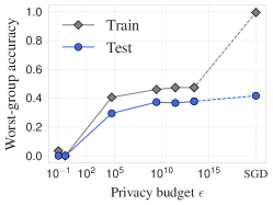
(a) Differential privacy as regularization

(b) $\ell_{2}$ regularization

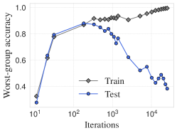
(c) Early-stopping as regularization

Figure 6: Regularization induces DG. The figure shows train/test worst-group accuracies as a function of regularization strength for SGD on CelebA, with different types of regularizers: differential privacy budget $\epsilon$, weight decay, and train time. For DP-SGD, $\epsilon=\infty$ represents standard SGD. For all types of regularizers, increasing the strength (left on x-axis) corresponds to a smaller generalization gap in worst-group accuracy.

Privacy, $\ell_{2}$ Regularization, and Early Stopping.

In Figure 6, we train a neural network on CelebA using DP-SGD, and decrease the “regularization strength” in several different ways: by increasing privacy budget $\epsilon$ (Figure 6a), decreasing the $\ell_{2}$ regularization (Figure 6b), or increasing the number of training iterations (Figure 6c). We then measure the gap in worst-group accuracy on train vs. test (Section E.2). We observe that for all regularizers, the gap between training and testing worst-group accuracy increases as the regularization is weakened.

Investigating $\ell_{2}$ Regularization in Depth.

In Figure 7, we show the training and testing worst-group accuracy with different strength of $\ell_{2}$ regularization and on different epochs (w/ and w/o $\ell_{2}$ regularization). We have three observations: (1) with properly tuned regularization parameter, the gap between training and testing worst-group accuracy can be narrowed, (2) the gap can start widening in very early stage of training, and (3) the testing worst-group accuracy can fluctuate largely, which highlights the importance of using validation set for early stopping in this task.

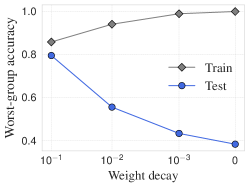
(a) CelebA

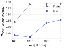
(b) UTKFace

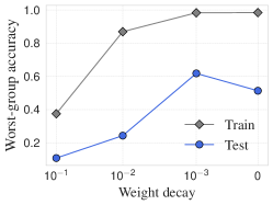
(c) iNat

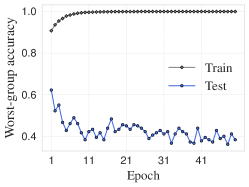
(d) CelebA (no reg.)

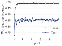
(e) UTKFace (no reg.)

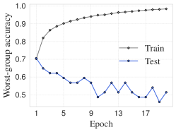
(f) iNat (no reg.)

(g) CelebA ($\ell_{2}$ reg.)

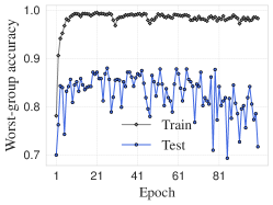
(h) UTKFace ($\ell_{2}$ reg.)

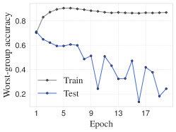
(i) iNat ($\ell_{2}$ reg.)

Figure 7: We show the training and testing worst-group accuracy with different strength of $\ell_{2}$ regularization and on different epochs (w/ and w/o $\ell_{2}$ regularization). The network is trained with IS-SGD on CelebA, UTKFace, and iNat. For (a), (b), and (c), we show the result of the last epoch. For (g), (h), and (i), we set weight decay to $0.01$.

E.4 Additional Details for Section 5.2

Figure 8 shows the accuracy disparity, test accuracy, and worst-group accuracy for CelebA, UTKFace, and iNat on DP-SGD and DP-IS-SGD.

The reason that UTKFace has a similar disparity between DP-SGD and DP-IS-SGD is likely because UTKFace has a relatively small difference in the number of training examples between the largest group and the smallest group. In UTKFace, the majority group has around seven times more examples than in the minority group, whereas in CelebA, this difference is $52\times$.

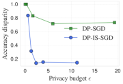
(a) CelebA

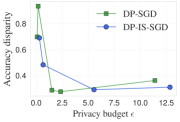
(b) UTKFace

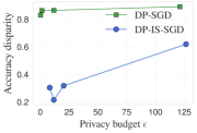
(c) iNat

(d) CelebA

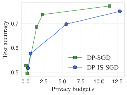
(e) UTKFace

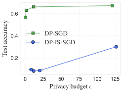
(f) iNat

(g) CelebA

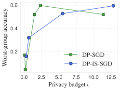
(h) UTKFace

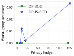
(i) iNat

Figure 8: The disparity (lower the better) and test accuracies of the models trained with DP-SGD and IW-SGD on three datasets. If we care about privacy, DP-IS-SGD improves disparate impact at most privacy budgets. For CelebA, we train the model for $30$ epochs. For UTKFace, we train for $100$ epochs. For iNat, we train for $20$ epochs. The GDP accountant is used to compute the privacy budget.

Comparison with DP-SGD-F Xu et al. [2021].

We did not manage to obtain good performance from DP-SGD-F on CelebA, UTKFace, and iNat, possibly because of the different domain—images—than tabular data considered by Xu et al. [2021]. To proceed with the comparison, we evaluate the algorithms on the census data—ADULT dataset Kohavi et al. [1996] (see Table 7 for dataset statistics)—that Xu et al. [2021] used in their work. As subgroups, we consider four intersectional groups composed of all possible values of the “sex” attribute and prediction class (an income higher/lower than 50k).

We show the results in Table 9. For a comparable epsilon value (0.69 for DP-SGD-F, and 0.7 for our DP-IS-SGD), we see that our method has smaller accuracy disparity (Eq. 2) across the groups, although also lower overall accuracy.

Table 9: DP-IS-SGD has lower disparity DP-SGD-F on ADULT and better accuracy at the same privacy level. The table shows the privacy level, maximum accuracy disparity across groups, and overall accuracy for all algorithms.

Algorithm	$\epsilon$	Accuracy disparity	Overall accuracy
SGD	-	$0.660\pm 0.000$	$0.836\pm 0.000$
DP-SGD	$0.6573$	$0.852\pm 0.005$	$0.802\pm 0.001$
DP-SGD-F	$0.6964$	$0.657\pm 0.023$	$0.832\pm 0.001$
DP-IS-SGD	$0.7059$	$0.246\pm 0.034$	$0.766\pm 0.010$

E.5 Additional Details for Section 5.3

We compare different algorithms, including SGD-$\ell_{2}$ and IW-SGD-$\ell_{2}$ as baselines, and two other algorithms, IS-SGD-$\ell_{2}$ Idrissi et al. [2022] and gDRO-$\ell_{2}$ Sagawa et al. [2019a] in terms of the group robustness. We set the learning rate as $0.001$ for CelebA, UTKFace, and iNat, $0.00002$ for MNLI, and $0.00001$ for CivilComments. We use the validation set to select the hyperparameters:

1. For SGD-$\ell_{2}$, IW-SGD-$\ell_{2}$, IS-SGD-$\ell_{2}$, and gDRO-$\ell_{2}$, we select the weight decay from $0.0001$, $0.01$, $0.1$, and $1.0$.

2. For DP-IS-SGD, we fix the gradient clipping to $1.0$ (except for iNat, where we set the value to $10.0$ as $1.0$ does not converge). We select the noise parameter from $1.0$, $0.1$, $0.01$, $0.001$ on CelebA and UTKFace, select the noise parameter from $0.0000001$, $0.000001$, $0.00001$, and $0.0001$ on iNat and select the noise parameter from $0.01$ and $0.001$ on CivilComments and MNLI.

3. For IW-SGD-n, IS-SGD-n, and gDRO-n, we select the standard deviation of the random noise from $0.001$, $0.01$, $0.1$, and $1.0$ on CelebA, UTKFace, and iNat, and we select standard deviation of the random noise from $0.00001$, $0.0001$, and $0.001$ on CivilComments and MNLI.

Statistical Concerns.

Although our results appear to be comparable to or better than SOTA, we caution readers about the exact ordering of methods due to high estimation variance: these benchmarks have small validation and test sets (e.g., CelebA has $182$ validation examples), and so hyperparameter tuning is subject to both overfitting and estimation error. For example, we observe validation accuracies which differ from their test accuracies by up to $5\%$ in our experiments. We attempt to mitigate this using three random train/val/test splits on CelebA, and avoid large hyperparameter sweeps, but this is not done in prior work.

E.6 Additional Details for Section 5.4

We use the CIFAR-10 dataset Krizhevsky et al. [2009], and ResNet-18 He et al. [2016] as the network architecture. We train the model to be robust against $L_{\infty}$ perturbations of at most $\gamma=8/255$ bound, which is a standard setup for adversarial training on this dataset. We vary $\sigma$ (noise parameter) from 0.0 (regular adversarial training without gradient noise) to 0.01. In addition, we compare the performance of noisy gradient to adversarial training with early stopping—a simple but effective approach for mitigating overfitting in adversarial training [Rice et al., 2020].

In this experiment, we measure robust accuracy and its respective generalization gap, thus setting $\ell((x,y),\theta)~{}\smash{\triangleq}~{}\mathbbm{1}[f_{\theta}(x)=y]$ to be the 0/1 loss.

Appendix F Author Contributions

BK proposed to leverage the connection between differential privacy and distribution generalization, and led the theory developments and algorithm analysis. Yao-Yuan Yang led the experiments, designed the experimental settings, and implemented the algorithms. Yaodong Yu contributed to the experiments, especially in the NLP settings, and helped benchmark baselines. The noisy-gradient algorithm is proposed by Yao-Yuan Yang and Yaodong Yu. JB contributed to the theory, in particular the algorithmic analysis, initial proof of the tightness of the bound, and formal connections to robust generalization and calibration. PN organized the team and managed the project, contributing in parts to the theory and experiments. All authors participated in framing the results and writing the paper.

References

- Abadi et al. [2016] Martin Abadi, Andy Chu, Ian Goodfellow, H Brendan McMahan, Ilya Mironov, Kunal Talwar, and Li Zhang. Deep learning with differential privacy. In Proceedings of the 2016 ACM SIGSAC conference on computer and communications security, 2016.
- Bagdasaryan et al. [2019] Eugene Bagdasaryan, Omid Poursaeed, and Vitaly Shmatikov. Differential privacy has disparate impact on model accuracy. In Advances in Neural Information Processing Systems 32: Annual Conference on Neural Information Processing Systems (NeurIPS), 2019.
- Barber and Duchi [2014] Rina Foygel Barber and John C Duchi. Privacy and statistical risk: Formalisms and minimax bounds. arXiv preprint arXiv:1412.4451, 2014.
- Bassily et al. [2016] Raef Bassily, Kobbi Nissim, Adam D. Smith, Thomas Steinke, Uri Stemmer, and Jonathan R. Ullman. Algorithmic stability for adaptive data analysis. In Proceedings of the 48th Annual ACM SIGACT Symposium on Theory of Computing, STOC, 2016.
- Bietti [2020] Elettra Bietti. From ethics washing to ethics bashing: a view on tech ethics from within moral philosophy. In Proceedings of the Conference on Fairness, Accountability, and Transparency, 2020.
- Borkan et al. [2019] Daniel Borkan, Lucas Dixon, Jeffrey Sorensen, Nithum Thain, and Lucy Vasserman. Nuanced metrics for measuring unintended bias with real data for text classification. In Companion proceedings of the 2019 World Wide Web conference, 2019.
- Bousquet and Elisseeff [2002] Olivier Bousquet and André Elisseeff. Stability and generalization. The Journal of Machine Learning Research, 2002.
- Bu et al. [2020a] Yuheng Bu, Shaofeng Zou, and Venugopal V Veeravalli. Tightening mutual information-based bounds on generalization error. IEEE Journal on Selected Areas in Information Theory, 2020a.
- Bu et al. [2020b] Zhiqi Bu, Jinshuo Dong, Qi Long, and Weijie J Su. Deep learning with gaussian differential privacy. Harvard data science review, 2020b.
- Buolamwini and Gebru [2018] Joy Buolamwini and Timnit Gebru. Gender shades: Intersectional accuracy disparities in commercial gender classification. In Conference on fairness, accountability and transparency, 2018.
- Byrd and Lipton [2019] Jonathon Byrd and Zachary Chase Lipton. What is the effect of importance weighting in deep learning? In Proceedings of the 36th International Conference on Machine Learning, ICML, 2019.
- Cao et al. [2019] Kaidi Cao, Colin Wei, Adrien Gaidon, Nikos Arechiga, and Tengyu Ma. Learning imbalanced datasets with label-distribution-aware margin loss. In Advances in Neural Information Processing Systems 32: Annual Conference on Neural Information Processing Systems (NeurIPS), 2019.
- Chaudhuri and Mishra [2006] Kamalika Chaudhuri and Nina Mishra. When random sampling preserves privacy. In Annual International Cryptology Conference. Springer, 2006.
- Chaudhuri et al. [2011] Kamalika Chaudhuri, Claire Monteleoni, and Anand D Sarwate. Differentially private empirical risk minimization. Journal of Machine Learning Research, 2011.
- Creager et al. [2021] Elliot Creager, Jörn-Henrik Jacobsen, and Richard Zemel. Environment inference for invariant learning. In Proceedings of the 38th International Conference on Machine Learning, ICML, 2021.
- Croce and Hein [2022] Francesco Croce and Matthias Hein. On the interplay of adversarial robustness and architecture components: patches, convolution and attention. arXiv preprint arXiv:2209.06953, 2022.
- Cummings et al. [2016] Rachel Cummings, Katrina Ligett, Kobbi Nissim, Aaron Roth, and Zhiwei Steven Wu. Adaptive learning with robust generalization guarantees. In Proceedings of the 29th Conference on Learning Theory, COLT, 2016.
- Cummings et al. [2019] Rachel Cummings, Varun Gupta, Dhamma Kimpara, and Jamie Morgenstern. On the compatibility of privacy and fairness. In Adjunct Publication of the 27th Conference on User Modeling, Adaptation and Personalization, 2019.
- Devlin et al. [2019] Jacob Devlin, Ming-Wei Chang, Kenton Lee, and Kristina Toutanova. BERT: Pre-training of deep bidirectional transformers for language understanding. In Proceedings of the 2019 Conference of the North American Chapter of the Association for Computational Linguistics: Human Language Technologies, Volume 1 (Long and Short Papers), 2019.
- Dong et al. [2019] Jinshuo Dong, Aaron Roth, and Weijie J Su. Gaussian differential privacy. arXiv preprint arXiv:1905.02383, 2019.
- Duchi et al. [2021] John C Duchi, Peter W Glynn, and Hongseok Namkoong. Statistics of robust optimization: A generalized empirical likelihood approach. Mathematics of Operations Research, 2021.
- Dwork et al. [2006] Cynthia Dwork, Frank McSherry, Kobbi Nissim, and Adam Smith. Calibrating noise to sensitivity in private data analysis. In Theory of cryptography conference. Springer, 2006.
- Dwork et al. [2014] Cynthia Dwork, Aaron Roth, et al. The algorithmic foundations of differential privacy. Found. Trends Theor. Comput. Sci., 2014.
- Dwork et al. [2015a] Cynthia Dwork, Vitaly Feldman, Moritz Hardt, Toniann Pitassi, Omer Reingold, and Aaron Roth. Generalization in adaptive data analysis and holdout reuse. In Advances in Neural Information Processing Systems 28: Annual Conference on Neural Information Processing Systems 2015, December 7-12, 2015, Montreal, Quebec, Canada, 2015a.
- Dwork et al. [2015b] Cynthia Dwork, Vitaly Feldman, Moritz Hardt, Toniann Pitassi, Omer Reingold, and Aaron Leon Roth. Preserving statistical validity in adaptive data analysis. In Proceedings of the 47th Annual ACM on Symposium on Theory of Computing, STOC, 2015b.
- Feldman and Zrnic [2021] Vitaly Feldman and Tijana Zrnic. Individual privacy accounting via a Renyi filter. In Advances in Neural Information Processing Systems 34: Annual Conference on Neural Information Processing Systems (NeurIPS), 2021.
- Geng et al. [2019] Quan Geng, Wei Ding, Ruiqi Guo, and Sanjiv Kumar. Optimal noise-adding mechanism in additive differential privacy. In The 22nd International Conference on Artificial Intelligence and Statistics, AISTATS, 2019.
- Goel et al. [2020] Karan Goel, Albert Gu, Yixuan Li, and Christopher Re. Model patching: Closing the subgroup performance gap with data augmentation. In 8th International Conference on Learning Representations, ICLR, 2020.
- Goodfellow et al. [2014] Ian J Goodfellow, Jonathon Shlens, and Christian Szegedy. Explaining and harnessing adversarial examples. arXiv preprint arXiv:1412.6572, 2014.
- Gretton et al. [2009] Arthur Gretton, Alex Smola, Jiayuan Huang, Marcel Schmittfull, Karsten Borgwardt, and Bernhard Schölkopf. Covariate shift by kernel mean matching. Dataset shift in machine learning, 2009.
- Haghifam et al. [2020] Mahdi Haghifam, Jeffrey Negrea, Ashish Khisti, Daniel M Roy, and Gintare Karolina Dziugaite. Sharpened generalization bounds based on conditional mutual information and an application to noisy, iterative algorithms. In Advances in Neural Information Processing Systems 33: Annual Conference on Neural Information Processing Systems (NeurIPS), 2020.
- Hardt et al. [2016] Moritz Hardt, Ben Recht, and Yoram Singer. Train faster, generalize better: Stability of stochastic gradient descent. In Proceedings of the 33nd International Conference on Machine Learning, ICML, 2016.
- Harris et al. [2020] Charles R. Harris, K. Jarrod Millman, Stéfan J. van der Walt, Ralf Gommers, Pauli Virtanen, David Cournapeau, Eric Wieser, Julian Taylor, Sebastian Berg, Nathaniel J. Smith, Robert Kern, Matti Picus, Stephan Hoyer, Marten H. van Kerkwijk, Matthew Brett, Allan Haldane, Jaime Fernández del Río, Mark Wiebe, Pearu Peterson, Pierre Gérard-Marchant, Kevin Sheppard, Tyler Reddy, Warren Weckesser, Hameer Abbasi, Christoph Gohlke, and Travis E. Oliphant. Array programming with NumPy. Nature, 2020.
- He et al. [2016] Kaiming He, Xiangyu Zhang, Shaoqing Ren, and Jian Sun. Deep residual learning for image recognition. In 2016 IEEE Conference on Computer Vision and Pattern Recognition, CVPR, 2016.
- Horn et al. [2018] Grant Van Horn, Oisin Mac Aodha, Yang Song, Yin Cui, Chen Sun, Alexander Shepard, Hartwig Adam, Pietro Perona, and Serge J. Belongie. The inaturalist species classification and detection dataset. In 2018 IEEE Conference on Computer Vision and Pattern Recognition, CVPR, 2018.
- Hu et al. [2018] Weihua Hu, Gang Niu, Issei Sato, and Masashi Sugiyama. Does distributionally robust supervised learning give robust classifiers? In Proceedings of the 35th International Conference on Machine Learning, ICML, 2018.
- Idrissi et al. [2022] Badr Youbi Idrissi, Martin Arjovsky, Mohammad Pezeshki, and David Lopez-Paz. Simple data balancing achieves competitive worst-group-accuracy. In Conference on Causal Learning and Reasoning, 2022.
- Kairouz et al. [2015] Peter Kairouz, Sewoong Oh, and Pramod Viswanath. The composition theorem for differential privacy. In Proceedings of the 32nd International Conference on Machine Learning, ICML, 2015.
- Koenecke et al. [2020] Allison Koenecke, Andrew Nam, Emily Lake, Joe Nudell, Minnie Quartey, Zion Mengesha, Connor Toups, John R Rickford, Dan Jurafsky, and Sharad Goel. Racial disparities in automated speech recognition. Proceedings of the National Academy of Sciences, 2020.
- Koh et al. [2021] Pang Wei Koh, Shiori Sagawa, Henrik Marklund, Sang Michael Xie, Marvin Zhang, Akshay Balsubramani, Weihua Hu, Michihiro Yasunaga, Richard Lanas Phillips, Irena Gao, et al. Wilds: A benchmark of in-the-wild distribution shifts. In Proceedings of the 38th International Conference on Machine Learning, ICML, 2021.
- Kohavi et al. [1996] Ron Kohavi et al. Scaling up the accuracy of Naive-Bayes classifiers: A decision-tree hybrid. In KDD, 1996.
- Krizhevsky et al. [2009] Alex Krizhevsky, Geoffrey Hinton, et al. Learning multiple layers of features from tiny images. 2009.
- Kulynych et al. [2022] Bogdan Kulynych, Mohammad Yaghini, Giovanni Cherubin, Michael Veale, and Carmela Troncoso. Disparate vulnerability to membership inference attacks. Proceedings on Privacy Enhancing Technologies, 2022.
- Kusner et al. [2017] Matt J. Kusner, Joshua R. Loftus, Chris Russell, and Ricardo Silva. Counterfactual fairness. In Advances in Neural Information Processing Systems 30: Annual Conference on Neural Information Processing Systems (NeurIPS), 2017.
- Li et al. [2012] Ninghui Li, Wahbeh Qardaji, and Dong Su. On sampling, anonymization, and differential privacy or, k-anonymization meets differential privacy. In Proceedings of the 7th ACM Symposium on Information, Computer and Communications Security, 2012.
- Liu et al. [2021] Evan Z Liu, Behzad Haghgoo, Annie S Chen, Aditi Raghunathan, Pang Wei Koh, Shiori Sagawa, Percy Liang, and Chelsea Finn. Just train twice: Improving group robustness without training group information. In Proceedings of the 38th International Conference on Machine Learning, ICML, 2021.
- Liu et al. [2015] Ziwei Liu, Ping Luo, Xiaogang Wang, and Xiaoou Tang. Deep learning face attributes in the wild. In 2015 IEEE International Conference on Computer Vision, ICCV 2015, Santiago, Chile, December 7-13, 2015, 2015.
- Loshchilov and Hutter [2019] Ilya Loshchilov and Frank Hutter. Decoupled weight decay regularization. In 7th International Conference on Learning Representations, ICLR, 2019.
- Madaio et al. [2020] Michael A Madaio, Luke Stark, Jennifer Wortman Vaughan, and Hanna Wallach. Co-designing checklists to understand organizational challenges and opportunities around fairness in ai. In Proceedings of the 2020 CHI Conference on Human Factors in Computing Systems, 2020.
- Madry et al. [2018] Aleksander Madry, Aleksandar Makelov, Ludwig Schmidt, Dimitris Tsipras, and Adrian Vladu. Towards deep learning models resistant to adversarial attacks. In 6th International Conference on Learning Representations, ICLR, 2018.
- Mohri et al. [2019] Mehryar Mohri, Gary Sivek, and Ananda Theertha Suresh. Agnostic federated learning. In Proceedings of the 36th International Conference on Machine Learning, ICML, 2019.
- Nakkiran and Bansal [2020] Preetum Nakkiran and Yamini Bansal. Distributional generalization: A new kind of generalization. arXiv preprint arXiv:2009.08092, 2020.
- Namkoong and Duchi [2016] Hongseok Namkoong and John C. Duchi. Stochastic gradient methods for distributionally robust optimization with f-divergences. In Advances in Neural Information Processing Systems 29: Annual Conference on Neural Information Processing Systems (NeurIPS), 2016.
- Neelakantan et al. [2015] Arvind Neelakantan, Luke Vilnis, Quoc V Le, Ilya Sutskever, Lukasz Kaiser, Karol Kurach, and James Martens. Adding gradient noise improves learning for very deep networks. arXiv preprint arXiv:1511.06807, 2015.
- Nelson and Reuben [2020] Boel Nelson and Jenni Reuben. SoK: Chasing accuracy and privacy, and catching both in differentially private histogram publication. Trans. Data Priv., 2020.
- pandas development team [2020] The pandas development team. pandas-dev/pandas: Pandas, 2020.
- Paszke et al. [2019] Adam Paszke, Sam Gross, Francisco Massa, Adam Lerer, James Bradbury, Gregory Chanan, Trevor Killeen, Zeming Lin, Natalia Gimelshein, Luca Antiga, et al. Pytorch: An imperative style, high-performance deep learning library. In Advances in Neural Information Processing Systems 32: Annual Conference on Neural Information Processing Systems (NeurIPS), 2019.
- Polyanskiy and Wu [2014] Yury Polyanskiy and Yihong Wu. Lecture notes on information theory. 2014.
- Pujol et al. [2020] David Pujol, Ryan McKenna, Satya Kuppam, Michael Hay, Ashwin Machanavajjhala, and Gerome Miklau. Fair decision making using privacy-protected data. In Proceedings of the Conference on Fairness, Accountability, and Transparency, 2020.
- Raskhodnikova et al. [2008] Sofya Raskhodnikova, Adam Smith, Homin K Lee, Kobbi Nissim, and Shiva Prasad Kasiviswanathan. What can we learn privately. In Proceedings of the 54th Annual Symposium on Foundations of Computer Science, 2008.
- Rice et al. [2020] Leslie Rice, Eric Wong, and Zico Kolter. Overfitting in adversarially robust deep learning. In Proceedings of the 37th International Conference on Machine Learning, ICML, 2020.
- Russo and Zou [2019] Daniel Russo and James Zou. How much does your data exploration overfit? controlling bias via information usage. IEEE Transactions on Information Theory, 2019.
- Sagawa et al. [2019a] Shiori Sagawa, Pang Wei Koh, Tatsunori B Hashimoto, and Percy Liang. Distributionally robust neural networks for group shifts: On the importance of regularization for worst-case generalization. arXiv preprint arXiv:1911.08731, 2019a.
- Sagawa et al. [2019b] Shiori Sagawa, Aditi Raghunathan, Pang Wei Koh, and Percy Liang. An investigation of why overparameterization exacerbates spurious correlations. In Proceedings of the 37th International Conference on Machine Learning, ICML, 2019b.
- Sanyal et al. [2022] Amartya Sanyal, Yaxi Hu, and Fanny Yang. How unfair is private learning? arXiv preprint arXiv:2206.03985, 2022.
- Shalev-Shwartz et al. [2010] Shai Shalev-Shwartz, Ohad Shamir, Nathan Srebro, and Karthik Sridharan. Learnability, stability and uniform convergence. The Journal of Machine Learning Research, 2010.
- Shokri et al. [2017] Reza Shokri, Marco Stronati, Congzheng Song, and Vitaly Shmatikov. Membership inference attacks against machine learning models. In IEEE symposium on security and privacy (SP), 2017.
- Steinke and Zakynthinou [2020] Thomas Steinke and Lydia Zakynthinou. Reasoning about generalization via conditional mutual information. In Conference on Learning Theory, 2020.
- Van Horn and Perona [2017] Grant Van Horn and Pietro Perona. The devil is in the tails: Fine-grained classification in the wild. arXiv preprint arXiv:1709.01450, 2017.
- Virtanen et al. [2020] Pauli Virtanen, Ralf Gommers, Travis E. Oliphant, Matt Haberland, Tyler Reddy, David Cournapeau, Evgeni Burovski, Pearu Peterson, Warren Weckesser, Jonathan Bright, Stéfan J. van der Walt, Matthew Brett, Joshua Wilson, K. Jarrod Millman, Nikolay Mayorov, Andrew R. J. Nelson, Eric Jones, Robert Kern, Eric Larson, C J Carey, İlhan Polat, Yu Feng, Eric W. Moore, Jake VanderPlas, Denis Laxalde, Josef Perktold, Robert Cimrman, Ian Henriksen, E. A. Quintero, Charles R. Harris, Anne M. Archibald, Antônio H. Ribeiro, Fabian Pedregosa, Paul van Mulbregt, and SciPy 1.0 Contributors. SciPy 1.0: Fundamental Algorithms for Scientific Computing in Python. Nature Methods, 2020.
- Wang [2017] Yu-Xiang Wang. Per-instance differential privacy. arXiv preprint arXiv:1707.07708, 2017.
- Wang et al. [2016] Yu-Xiang Wang, Jing Lei, and Stephen E Fienberg. Learning with differential privacy: Stability, learnability and the sufficiency and necessity of erm principle. The Journal of Machine Learning Research, 2016.
- Wasserman and Zhou [2010] Larry Wasserman and Shuheng Zhou. A statistical framework for differential privacy. Journal of the American Statistical Association, 2010.
- Williams et al. [2018] Adina Williams, Nikita Nangia, and Samuel Bowman. A broad-coverage challenge corpus for sentence understanding through inference. In Proceedings of the Conference of the North American Chapter of the Association for Computational Linguistics: Human Language Technologies, Volume 1 (Long Papers), 2018.
- Wolf et al. [2019] Thomas Wolf, Lysandre Debut, Victor Sanh, Julien Chaumond, Clement Delangue, Anthony Moi, Pierric Cistac, Tim Rault, Rémi Louf, Morgan Funtowicz, et al. Huggingface’s transformers: State-of-the-art natural language processing. arXiv preprint arXiv:1910.03771, 2019.
- Xu and Raginsky [2017] Aolin Xu and Maxim Raginsky. Information-theoretic analysis of generalization capability of learning algorithms. In Advances in Neural Information Processing Systems 30: Annual Conference on Neural Information Processing Systems, 2017.
- Xu et al. [2021] Depeng Xu, Wei Du, and Xintao Wu. Removing disparate impact on model accuracy in differentially private stochastic gradient descent. In Proceedings of the 27th ACM SIGKDD Conference on Knowledge Discovery & Data Mining, 2021.
- Yang et al. [2020] Yao-Yuan Yang, Cyrus Rashtchian, Hongyang Zhang, Ruslan Salakhutdinov, and Kamalika Chaudhuri. A closer look at accuracy vs. robustness. In Advances in Neural Information Processing Systems 33: Annual Conference on Neural Information Processing Systems (NeurIPS), 2020.
- Yousefpour et al. [2021] Ashkan Yousefpour, Igor Shilov, Alexandre Sablayrolles, Davide Testuggine, Karthik Prasad, Mani Malek, John Nguyen, Sayan Ghosh, Akash Bharadwaj, Jessica Zhao, Graham Cormode, and Ilya Mironov. Opacus: User-friendly differential privacy library in PyTorch. arXiv preprint arXiv:2109.12298, 2021.
- Yu et al. [2022] Chaojian Yu, Bo Han, Li Shen, Jun Yu, Chen Gong, Mingming Gong, and Tongliang Liu. Understanding robust overfitting of adversarial training and beyond. In Proceedings of the 39th International Conference on Machine Learning, ICML, 2022.
- Zhang et al. [2019] Hongyang Zhang, Yaodong Yu, Jiantao Jiao, Eric Xing, Laurent El Ghaoui, and Michael Jordan. Theoretically principled trade-off between robustness and accuracy. In Proceedings of the 36th International Conference on Machine Learning, ICML, 2019.
- Zhang et al. [2020] Jingzhao Zhang, Aditya Menon, Andreas Veit, Srinadh Bhojanapalli, Sanjiv Kumar, and Suvrit Sra. Coping with label shift via distributionally robust optimisation. arXiv preprint arXiv:2010.12230, 2020.
- Zhang et al. [2017] Zhifei Zhang, Yang Song, and Hairong Qi. Age progression/regression by conditional adversarial autoencoder. In 2017 IEEE Conference on Computer Vision and Pattern Recognition, CVPR, 2017.