Accelerating Attention through
Gradient-Based Learned Runtime Pruning

Abstract.

Self-attention is a key enabler of state-of-art accuracy for various transformer-based Natural Language Processing models. This attention mechanism calculates a correlation score for each word with respect to the other words in a sentence. Commonly, only a small subset of words highly correlates with the word under attention, which is only determined at runtime. As such, a significant amount of computation is inconsequential due to low attention scores and can potentially be pruned. The main challenge is finding the threshold for the scores below which subsequent computation will be inconsequential. Although such a threshold is discrete, this paper formulates its search through a soft differentiable regularizer integrated into the loss function of the training. This formulation piggy backs on the back-propagation training to analytically co-optimize the threshold and the weights simultaneously, striking a formally optimal balance between accuracy and computation pruning. To best utilize this mathematical innovation, we devise a bit-serial architecture, dubbed LeOPArd, for transformer language models with bit-level early termination microarchitectural mechanism. We evaluate our design across 43 back-end tasks for MemN2N, BERT, ALBERT, GPT-2, and Vision transformer models. Post-layout results show that, on average, LeOPArd yields 1.9$\times$and 3.9$\times$speedup and energy reduction, respectively, while keeping the average accuracy virtually intact ($<\,0.2\%$ degradation).

1. Introduction

Natural Language Processing (NLP) defines the frontier for Artificial Intelligence (AI) as it is even central to the Turing Test (tur, 2021). The recent advent of the self-attention mechanism (Vaswani et al., 2017) enabled unprecedented successes in the field of NLP, shifting the focus of deep learning from convolutional neural networks towards Transformer models in various domains (Jumper et al., 2021; Katharopoulos et al., 2020; Brown et al., 2020; Dai et al., 2019; Kenton and Toutanova, 2019; Lan et al., 2019; Raffel et al., 2019; Liu et al., 2019; Ye et al., 2019; Child et al., 2019; Veličković et al., 2017). The self-attention mechanism calculates a score to measure the correlation between a word and all the other words in a subtext. The subtext is the collection of all the words, which is captured by the attention mechanism. Therefore, it quantifies the context of the word under attention with respect to its subtext.

Intuitively, a word can bear multiple connotations, of which only one is expressed in its proximate context. Usually, few keywords define the context and therefore, a significant amount of computation will be inconsequential. The attention score for a word determines highly correlated words; the rest are merely irrelevant. There exists a threshold that differentiates between the scores of the words that need to be considered and those that do not define the context and are thus inconsequential. Because each attention layer identifies a distinct context of the target sentence, such a threshold needs to be defined on a per-layer basis to maintain model accuracy. Recent research has leveraged this insight and proposed several techniques that skip computation if a threshold is not met (Wang et al., 2021; Ham et al., 2021; Tambe et al., 2021; Ham et al., 2020). Clearly, skipping computation negatively impacts model accuracy, which is also dependent on the value of the thresholds. Therefore, establishing the right thresholds is crucial for the efficacy of the runtime computation pruning methods. However, the literature (Wang et al., 2021; Ham et al., 2021; Tambe et al., 2021; Ham et al., 2020) has relied on heuristics, statistical sampling, or human input that do not provide reliable expected accuracy.

In contrast, this paper formulates the problem of finding thresholds for the attention layers as a regularizer that amends the loss function of the transformer model. Our technique is robust even though the threshold values are discrete and cannot be directly optimized through gradient-based approaches. A key contribution of this work is to formulate finding the layer-wise pruning thresholds as a differentiable regularizer. This formulation leverages the gradient-based back-propagation algorithm to mathematically co-optimize the threshold values and weight parameters. This approach unblocks simultaneous co-optimization of the two conflicting objectives of maximizing the pruning rate of the computations while minimizing the accuracy loss. In addition, this analytical technique strikes a formally optimal balance between accuracy and computation pruning. Note that the current Cambrian explosion of deep learning hinges upon two main algorithmic innovations. First, changing the activation function of perceptrons from a non-differentiable step function to the continuous smooth sigmoid function (Rumelhart et al., 1986) enabled back-propagation and multi-layer neural networks and ended the first AI winter (ai_, 2021). Second, solving the vanishing gradients problem (Kolen and Kremer, 2001) has resulted in stable training deep neural networks that have taken the IT industry by storm. The proposed approach is analytical and therefore mathematically sound, and does not rely on limited empirical evidence. The solution also guarantees the same generality and optimality that are essential for training the machine learning model itself.

In this paper, we apply these algorithmic innovations to learn self-attention thresholds in a gradient-based fashion. At runtime, the attention scores below the learned threshold are replaced by $-\infty$ to void their impact on the attention layer’s outputs. As such, the preceding computation can be pruned early when the result is below the threshold. We devise a bit-serial architecture, called LeOPArd , to maximize the benefits by terminating computation even before pruning the following calculation. This design reduces computation at the finest granularity possible (bit level), hence offering benefits beyond pruning. Our hardware mechanism for early termination is exact and does not cause any accuracy degradation. At the bit level, it can be determined ahead of calculation completions if the partial result of the dot-product can ever exceed the threshold. Therefore, another advance of this paper is leveraging arithmetic insights for early termination in the microarchitecture without approximation.

We evaluate the effectiveness of our gradient-based algorithmic innovation and the proposed bit-level arithmetic properties by designing and implementing the LeOPArd accelerator in hardware. We synthesize and generate layout for a prototype of the LeOPArd accelerator implementation in a 65 nm process technology and characterize its speed and energy consumption under various settings. We evaluate various state-of-the-art transformer models, including BERT, GPT-2 and Vision-Transformer, and datasets forming a benchmark suite of 43 language and vision processing tasks. On average, the designed accelerator offers 1.9$\times$ and 3.9$\times$ speedup and energy reduction, respectively, compared to a baseline design without pruning and bit-level early termination support under an iso-area setting. LeOPArd’s notable pruning rate can unlock more benefits, if more chip area budget (15%) is available. Given this extra area budget, our accelerator’s benefits increase to 2.4$\times$and 4.0$\times$speedup and energy reduction, respectively. To better understand the sources of these improvements, we also distinguish between the effects of runtime computation pruning and bit-level early termination on energy savings. Our study across the target models shows that, on average, out of the 3.9$\times$ energy reduction, 2.1$\times$ stems from runtime computation pruning and 1.8$\times$ emerges from bit-level early termination. We also compare LeOPArd to two state-of-the-art accelerators for self-attention mechanism, $A^{3}$ (Ham et al., 2020) and SpAtten (Wang et al., 2021), which support runtime pruning. However, neither accelerator provides analytical support or guarantee for model accuracy, only relying on heuristic approximations. The results from our evaluations suggest that formulating runtime pruning as a gradient-based optimization can unlock significant benefits, while guaranteeing inference accuracy.

2. Background and Motivation

2.1. Self-Attention Mechanism

“Self-attention” is a mechanism to find the relation between a word to all the other words in a sentence (Vaswani et al., 2017; Choromanski et al., 2020). To compute this relation, we first project each word to a vector with $d_{w}$ dimensions, so-called embedding. Given a sentence with $s$ words, this projection creates a matrix $\mathcal{X}$ with $s\times{d_{w}}$. Then, these word embeddings are multiplied into query weight matrix ($W^{\mathcal{Q}}$), key weight matrix ($W^{\mathcal{K}}$), and value weight matrix ($W^{\mathcal{V}}$), each with $d_{w}\times{d}$ dimensions as follows:

(1) $$\mathcal{Q}_{s\times{d}}=\mathcal{X}\times\mathcal{W^{\mathcal{Q}}};\quad\mathcal{K}_{s\times{d}}=\mathcal{X}\times\mathcal{W^{\mathcal{K}}};\quad\mathcal{V}_{s\times{d}}=\mathcal{X}\times\mathcal{W^{\mathcal{V}}}\\$$

Given the query ($\mathcal{Q}$) and key ($\mathcal{K}$) matrices, a self-attention $Score$ matrix is calculated as follows:

(2) $$\mathrm{Score}_{s\times{s}}=\mathcal{Q}\times\mathcal{K}^{T}$$

where each element $s_{ij}$ in the self-attention $Score$ matrix indicates the relation between word_i and word_j in the input sentence. The $Score$ values are generally scaled down by ($\times 1/\sqrt{d}$) before the next step to enable stable gradients during training (Vaswani et al., 2017). To ensure that the self-attention $Score$s are positive and adding up to one, “softmax” is applied to each row of $\mathrm{Score}$ matrix as follows:

(3) $$\begin{split}\mathcal{P}_{s\times{s}}&=\mathrm{Softmax}(\mathrm{Score})\end{split}$$

Softmax outputs indicate a $\mathrm{probability}$ estimation of the input words’ relation. The self-attention values are calculated as follows:

(4) $$\mathrm{Att}_{s\times{}d}=\mathcal{P}\times\mathcal{V}$$

Generally, each attention layer consists of multiple heads each with dedicated $W^{\mathcal{Q}}$, $W^{\mathcal{K}}$, and $W^{\mathcal{V}}$ weight matrices. Each head presumably captures different dependencies between the token embeddings. In this case, the attention values (Equation 4) from each head are concatenated and projected into an attention matrix of size $s\times{}d_{w}$ using a weight matrix $\mathcal{W}^{o}_{({d}\times{}h)\times{d_{w}}}$ as follows:

(5) $$\mathrm{Multi-Head\;Att}_{s\times{}d_{w}}=\mathrm{Concat}(\mathrm{Att}_{1},\ \mathrm{Att}_{2},\ \cdot\cdot\cdot,\ \mathrm{Att}_{h})\times\mathcal{W}^{o}$$

where $\mathrm{Concat}$ operation concatenates the $\mathrm{Att}$ output matrix from each head to generate a $(s\times{}(d\times{}h))$-matrix.

2.2. Gradient-Based Optimization and Regularization

Gradient-based optimization. Training neural networks are formulated as an optimization problem of a predefined loss function. These loss functions are generally non-convex and have a manifold consisting of different local optima which makes the training of neural networks challenging. To alleviate the complexity of optimizing loss functions, it is common to use gradient-based methods (Robbins and Monro, 1951; Kingma and Ba, 2014). Using these gradient-based methods institute defining differentiable loss functions, such as cross-entropy (Murphy, 2012) or Kullback-Leibler divergence (Kullback and Leibler, 1951) which is prevalent in self-attention models (Kenton and Toutanova, 2019; Vaswani et al., 2017; Sukhbaatar et al., 2015).

Regularization in loss function. To impose certain constraints on the model parameters, such as improved generalization (Krogh and Hertz, 1992; Zou and Hastie, 2005; Srivastava et al., 2014) and introducing sparsity (Gale et al., 2019; Srinivas et al., 2017; Azarian et al., 2020), it is common to use regularizer as part of the loss function. However, using gradient-based methods for training mandates these regularizers to be framed as additional differentiable terms to the loss. This differentiability constraint for employing gradient-based methods introduces a unique challenge for supporting constraints that are not inherently differentiable.

2.3. Motivation

Analyzing the computations for self-attention layers, it is apparent that the main computation cost is associated to $\mathrm{Score}$ (Equation 2) and attention computations (Equation 4) that necessitates the multiplications of two matrices with $s\times{}d$ dimensions, each with time complexity of $\mathcal{O}(s^{2}d)$. These complexities translate to quadratic raise in computation cost and storage as the number of input tokens increases. As such, prior work aims to reduce the time and space complexity of these operations both from the algorithmic (Choromanski et al., 2020; Wang et al., 2020; Beltagy et al., 2020; Zaheer et al., 2020; Child et al., 2019) and hardware perspectives (Wang et al., 2021; Ham et al., 2021; Kao et al., 2021; Stevens et al., 2021; Ham et al., 2020). In this work, we propose an alternative pruning mechanism that learns the threshold as part of training. Our proposed technique prunes away unimportant $Score$s, hence eliminating the ineffectual computations of “softmax($\cdot$)” in Equation 3 and “$\times\mathcal{V}$” in Equation 4. In addition, to further cut down the computations of $Score$s (Equation 2), we employ a unique early-compute termination without impacting the model accuracy.

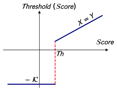
(a) Ideal Pruning

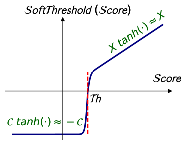
(b) Pruning with Soft Threshold

Figure 1. Pruning operation on attention $Score$: (a) ideal magnitude-based pruning, (b) proposed differentiable pruning operation with soft threshold.

3. Algorithmic Optimizations for Sparse Attention

The section overviews the algorithmic optimizations for inducing sparsity in attention layers. We first introduce an online pruning method that eliminate unimportant attention layer computations as early as possible, right after $Score$ calculations (e.g. $\mathcal{Q}\times\mathcal{K}{\color[rgb]{0,0,0}^{T}}$), to increase the realized performance benefits. Particularly, our method sets the layer-wise pruning thresholds as trainable parameters and jointly fine-tune the model parameters and learn the pruning thresholds as part of a light fine-tuning step. Then, our method compares the $Score$ = $\mathcal{Q}\times\mathcal{K}{\color[rgb]{0,0,0}^{T}}$ values against the learned pruning thresholds per attention layer and prunes the ones that satisfy the pruning criteria. Note that, in contrast to prior learned weight pruning method for image classification models  (Azarian et al., 2020), the pruning criteria in our work is content-dependant and is applied adaptively based on the calculated $Score$ values. That means the induced sparsity in attention layers by our approach varies from one content to another content. As our results indicate (See Section 5), the adaptive and content-dependant nature of our pruning method enables high sparsity in attention computations while yielding virtually no accuracy loss.

3.1. Learned Per-Layer Pruning

Learning per-layer pruning thresholds for attention layers consists of three main challenges. First, the search space of threshold values is complex and computationally intractable for exhaustive exploration. For example, BERT-L model has 24 layers creating a total of 24 threshold parameters, each of which can take any continuous value. Second, simply sweeping the threshold values as a one-time fine-tuning step could negatively affect the model accuracy (Ham et al., 2020; Wang et al., 2021). To mitigate these challenges, we propose to jointly fine-tune the model parameters and learn the threshold values as a light fine-tuning step with the joint objective of increasing model sparsity and retaining the baseline model accuracy. However, training the threshold values with the inherently non-differentiable pruning operation poses a unique challenge for gradient-based learned methods. For this, we use an approximate differentiable pruning operation and devise a surrogate regularizer to reinforce sparsity as part of the model loss function. In the following paragraphs, we expound our learned pruning method that couples two design principles, namely “pruning with soft threshold” and “surrogate L₀ regularization”.

Pruning with soft threshold. Figure 1a demonstrates an ideal pruning operation for $Score$ values (e.g. $Score$ = $\mathcal{Q}\times\mathcal{K}{\color[rgb]{0,0,0}^{T}}$, where $\mathcal{Q}$ and $\mathcal{K}$ are $d$-dimension vectors corresponding to a single word). The $Score$ values greater than $\mathcal{T}h$ remain unchanged and those less than $\mathcal{T}h$ are clipped to a large negative number. As the pruning operation is followed by a “softmax($\cdot$)”, setting the $Score$ values below $\mathcal{T}h$ to a large negative number makes the output of the softmax operation sufficiently close to zero. Hence, the large negative numbers are pruned out of the following multiplication into $\mathcal{V}$. However, using this pruning operation as part of a gradient-based training method is not straightforward due to its discontinuity at $X$ = $\mathcal{T}h$.

To circumvent the non-differentiality in the pruning operation, we propose to replace this operation with an approximate function that instead uses a soft threshold (shown in Figure 1b) as follows:

(6) $$\mathrm{SoftThreshold(x)}=\begin{cases}{x~{}\mathrm{tanh}(s(x-\mathcal{T}h))},&x\geq\mathcal{T}h\\ {c~{}\mathrm{tanh}(s(x-\mathcal{T}h))},&x<\mathcal{T}h\end{cases}$$

By assigning a reasonably large value to $s$, the shape of $tanh(\cdot)$ around $\mathcal{T}h$ becomes sharper and enables the learning gradients to effectively flow around this region. Supporting the learning gradients to flow at the vicinity of $\mathcal{T}h$ allow the gradient-based learning algorithm to either push down the model parameters (e.g. $\mathcal{Q}$ and $\mathcal{K}$) below the threshold or lift them above the threshold according to their contributions to the overall model accuracy.

Outside the vicinity of $\mathcal{T}h$, the $tanh(\cdot)$ asymptotically approaches one and the “SoftThreshold” function simply becomes $\approx{x}$ and $\approx{-c}$ for values $\geq$ $\mathcal{T}h$ and ¡ $\mathcal{T}h$, respectively, which are close approximations of the original pruning operation. In our experiments, we empirically find that setting $c$ = 1000 and $s$ = 10 yield a good approximation for pruning and enables robust training.

Differentiable surrogate L₀ regularization. Using soft threshold as the sole force of pruning does not necessarily increase sparsity. Intuitively, the training method may just simply lower the threshold to be a small value, which translates to lower sparsity to maintain high model accuracy. Imposing such constraints to gradient-based methods are generally achieved through adding a regularizer term to the loss function. A common method to explicitly penalize the number of non-zero model parameters is to use L₀ regularizer on model parameters in the loss function as follows:

(7) $$&\mathrm{L}_{tot}(\theta)=\frac{1}{N}\Big{(}{\sum}_{i=1}^{N}\mathcal{L}\big{(}A(x_{i};~{}\theta),~{}y_{i}\big{)}\Big{)}+\lambda||\theta||_{0}\\ ||\theta||_{0}={\sum}_{j=1}^{|\theta|}\mathbbm{1}[\theta_{j}\neq 0]$$

where $\mathcal{L}$ is the model loss function, $A(\cdot)$ is the model output for given input $x_{i}$ and model parameters $\theta$, $y_{i}$ is the corresponding labeled data, $\lambda$ is the balancing factor for L₀ regularizer, and $\mathbbm{1}$ is the identity operator that counts the number of non-zero parameters.

Similar to “Threshold” function, L₀ regularizer suffers from the same non-differentiability limitation. To mitigate this, Louizos et al. (Louizos et al., 2017) uses a reparameterization of model parameters to compute the training gradients. While this reparameterization technique yields state-of-the-art results for Wide Residual Networks (Zagoruyko and Komodakis, 2016) and small datasets, a recent study (Gale et al., 2019) shows that this reparameterization trick performs inconsistently for large-scale tasks such as attention models. In this work, we propose a simple alternative method that uses a differentiable surrogate L₀ regularization for the pruning of $Score$ values in attention layers as follows:

(8) $$&||\theta||_{0}={\sum}_{j=1}^{|score|}\mathbbm{1}[\mathrm{score}_{j}>-c]\\ ||\theta||_{0}\approx{\sum}_{j=1}^{|score|}\mathrm{sigmoid}({k(\mathrm{score}_{j}+c-\alpha}))$$

where $k$ = 100 and $\alpha$ = 1. Using these parameters forces the output of sigmoid($\cdot$) to asymptotically approach one for unpruned $Score$ values and zero for the pruned ones, which are already bounded to $-~{}c$ as shown in Equation 6. As such, the proposed differentiable surrogate L₀ regularizer is a close approximation of the original L₀ regularizer in Equation 8 (a).

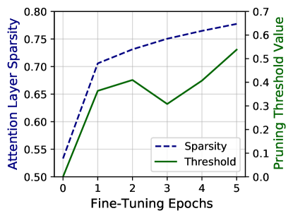
(a) Sparsity and Pruning Threshold

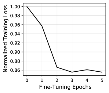
(b) Normalized Training Loss

Figure 2. An example (a) attention layer sparsity and its corresponding pruning threshold values and (b) normalized training loss as fine-tuning epochs progress for BERT-L model on QNLI task from GLUE benchmark.

Pruning mechanism. We apply our gradient-based learned pruning as a light fine-tuning step based on the previously proposed design principles: (1) pruning with soft threshold and (2) differentiable surrogate L₀ regularization. We employ the pre-trained attention models with the proposed modified loss function (e.g. original loss function and the surrogate L₀ regularizer) to jointly fine-tune the model parameters and learn the per-layer pruning thresholds. Using the proposed soft threshold mechanism in the fine-tuning step allows the gradient-based learning method to adjust the model parameters smoothly at the vicinity of the $\mathcal{T}h$ value. That is, pushing down the non-important model parameters below threshold values and lifting up the important model parameters above it. One of the main benefits of using the proposed differentiable approach is enabling the model parameters to freely switch between prune and unpruned region. For all the studied attention models, we initialize the threshold values to zero and run the fine-tuning for up to five epochs.

Figure 2 demonstrates an example sparsity, threshold values, and normalized training loss curves for BERT-B model on QNLI task from the GLUE benchmark. Figure 2a shows that as fine-tuning epochs progress, both the sparsity and threshold values increase owing to the effectiveness of our joint co-training of sparsity and model parameters. The flexibility afforded by the joint co-training is further illustrated at the third epoch, where the sparsity continues to increase despite the corresponding decrease in the threshold value. Additionally, Figure 2b shows the decreasing trend of normalized training loss over the course of fine-tuning epochs.

3.2. Bit-Level Early-Compute Termination

The learned pruning offers a unique opportunity to further improve the LeOPArd performance through bit-serial $\mathcal{Q}\times\mathcal{K}{\color[rgb]{0,0,0}^{T}}$ computation. If our system can anticipate that the final result of $\mathcal{Q}\times\mathcal{K}{\color[rgb]{0,0,0}^{T}}$ computation is below the learned pruning threshold, the ongoing bit-serial computations can be terminated. However, this early-termination mechanism poses a key challenge in our design. As we desire to maintain the baseline model accuracy, the early-termination mechanism must not tamper with the computational correctness of attention layers. To address this, we propose to compute and add a dynamically adjusted conservative margin value to the partial sum during the bit-serial computations. The role of this margin is to account for the maximum potential increase in the remaining $\mathcal{Q}\times\mathcal{K}{\color[rgb]{0,0,0}^{T}}$ computations. If the addition of the partial sum values and the margin still falls below the learned pruning threshold value, the computations are terminated and the corresponding $\mathcal{Q}\times\mathcal{K}{\color[rgb]{0,0,0}^{T}}$ is simply pruned. In the following paragraph, we illustrate the proposed early-compute termination with a conservative margin.

Early-compute termination for dot-product operation. Figure 3 depicts the flow for a $\mathcal{Q}\times\mathcal{K}{\color[rgb]{0,0,0}^{T}}$ dot-product computation, each with four elements. $\mathcal{K}$ elements are placed in bit-serial format vertically from MSB $\rightarrow$ LSB, whereas $\mathcal{Q}$ values are stored in full-precision fixed-point format. In this example, the threshold value is set to five. For simplicity, we assume the computation is performed in sign-magnitude form, $k_{s}$ represents the sign-bit for $\mathcal{K}$ vector, and the absolute values of $\mathcal{K}$ elements are less than one.

In the first cycle, the elements with concordant signs, ($k^{0}$, $q^{0}$) and ($k^{1}$, $q^{1}$), are used for margin initialization. The intuition here is that only the multiplications of elements with concordant signs can contribute positively to the final dot-product result. Multiplications of elements with opposing signs are ignored to keep the margin conservative and eliminate wrongful early compute terminations. As shown in the table of Figure 3, both the product of $k^{2}$ and the $q$ vector as well as the margin are updated. The margin is adjusted to accommodate the largest possible positive contribution to the final value. In the second cycle, because the sum of $\mathcal{P}_{2}$ and $\mathcal{M}_{2}$ dips below the threshold, the computation process terminates. That is, the subsequent cycles (highlighted in gray) are no longer performed. Note that, with the proposed margin computation, we ensure that no approximation is introduced in the attention layers. Next section discusses the hardware realization for this proposal.

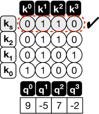
(a) Cycle = 1

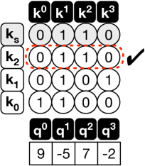
(b) Cycle = 2

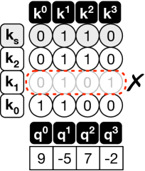
(c) Cycle = 3

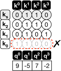
(d) Cycle = 4

Cycle	$\mathcal{P}$ = Partial Sum	$\mathcal{M}$ = Conservative Margin	Early Termination? ($\mathcal{T}h$ = 5)
1	$\mathcal{P}_{1}=0$	$\mathcal{M}_{1}=(9+5)(2^{-1}+2^{-2}+2^{-3})=12.25$	$\mathcal{P}_{1}+\mathcal{M}_{1}=12.25\geq 5$; ✗
2	$\mathcal{P}_{2}=\mathcal{P}_{1}+(5-7)2^{-1}=-1$	$\mathcal{M}_{2}=(9+5)(2^{-2}+2^{-3})=5.25$	$\mathcal{P}_{2}+\mathcal{M}_{2}=4.25<$ $5$; ✔
3	$\mathcal{P}_{3}=\mathcal{P}_{2}+(5-2)2^{-2}=-0.25$	$\mathcal{M}_{3}=(9+5)(2^{-3})=1.75$	$\mathcal{P}_{3}+\mathcal{M}_{3}=1.5<$ $5$;
4	$\mathcal{P}_{4}=\mathcal{P}_{3}+(9+5)2^{-3}=1.5$	$\mathcal{M}_{4}=0$	$\mathcal{P}_{4}+\mathcal{M}_{4}=1.5<$ $5$;

Figure 3. High-level overview of early-compute termination for dot-product operation $\mathcal{Q}\times\mathcal{K}{\color[rgb]{0,0,0}^{T}}$. In this example, $\mathcal{K}$ is represented in bit-serial format, whereas $\mathcal{Q}$ is in full-precision fixed-point format. In Figure (a-d) each column illustrate one element of $\mathcal{K}$ vector and each row represents its corresponding bits (MSB $\rightarrow$ LSB). K_s indicates the sign bit. For simplicity, $\mathcal{K}$ elements are scaled to be between -1.0 and +1.0. The table shows the partial sum values after each cycle.

4. LeOPArd Hardware architecture

We design LeOPArd hardware while considering the following requirements based on our algorithmic optimizations:

1. Leveraging the layer threshold values to detect the unpruned $Score$s and their corresponding indices in the output matrix.

2. Using bit-serial processing to early-stop the computation of pruned $Score$s and associated memory access .

3. Processing the $\times\mathcal{V}$ operation for only un-pruned $Score$s to minimize operations while achieving high compute utilization.

4.1. Overall Architecture

Due to abundant available parallelism in multi-head attention layers, we design a tile-based architecture for LeOPArd, where attention heads are partitioned across the tiles, and the operations in the tiles are independent of each other on their corresponding heads. Figure 4 illustrates the high-level microarchitecture of a single LeOPArd tile. Each tile comprises two major modules to process the computations of attention layers:

1. A front-end unit, dubbed Query Key Processing Unit (QK-PU), that streams in the $\mathcal{Q}$ vectors (row by row from the $Q$ matrix, where each row corresponds to a word) from the off-chip memory, reads $\mathcal{K}$s from a local buffer, and performs vector-matrix multiplication between a $\mathcal{Q}$ vector and a $\mathcal{K}$ matrix. This unit also encompasses a 1-D array of bit-serial dot-product units, QK-DPUs, each of which equipped with logic to early-stop the computations based on the pruning threshold values and forward the unpruned $Score$s and their indices to the second stage.

2. A back-end unit, dubbed Value Processing Unit (V-PU), that performs softmax operations on the important un-pruned $Score$s to generate probability, and subsequently performs weighted-summation of the $\mathcal{V}$ vectors read from a local buffer to generate the final output of the attention layer.

The front- and back-end stages are connected to each other through a set of FIFOs that store the survived $Score$s and their corresponding indices. The front-end unit employs multiple ($N_{\mathrm{QK}}$) QK-DPUs while sharing the single V-PU in consideration of high pruning rate during the processing in the front-end stage. If the front-end finished the computation with current $\mathcal{Q}$ vector, but the back-end is still working on the previous $\mathcal{Q}$ vector, the front-end unit is stalled until the completion of back-end unit.

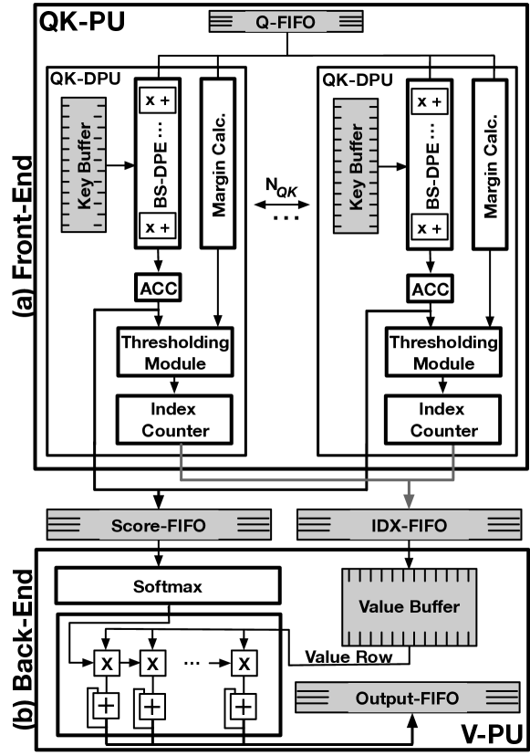
Figure 4. Overall microarchitecture of a LeOPArd tile.

As the choice of $N_{\mathrm{QK}}$ is a key factor to maximize the overall throughput and back-end resource utilization, we explore this design space in Section 5.4, which leads to two choices of $N_{\mathrm{QK}}=$ 6 and 8 by focusing on area efficiency and higher utilization, respectively. Before the operation begins, all the $\mathcal{K}$ and $\mathcal{V}$ matrices are fetched from off-chip memory and stored on on-chip buffers, while the $\mathcal{Q}$ vectors are steamed in. Since the vectors are re-used by the number of sequence elements (e.g., 512 in BERT), DRAM costs are amortized.

4.2. Online Pruning Hardware Realization via Bit-serial Execution

As discussed in Section 3, to realize the pruning of redundant $Score$s during runtime and even earlier termination with bit-level granularity, we design LeOPArd front-end unit (depicted in Figure 4-(a)) as a collection of bit-serial dot-product units (QK-DPU).

Overall front-end execution flow. To perform the $Score$ computations, the $\mathcal{Q}$ vectors are read sequentially from Q-FIFO and then broadcasted to each QK-DPU, while each QK-DPU reads a $\mathcal{K}$ vector from its local Key Buffer and performs a vector dot-product operation. As such, while the $\mathcal{Q}$ vector is shared amongst the QK-DPUs, the $\mathcal{K}$ matrix is partitioned along its columns and is distributed across the Key Buffers. Each QK-DPU performs the dot-product operations in a bit-serial mode, where the $\mathcal{K}$ elements are processed in bit-sequential manner and the $\mathcal{Q}$ elements are processed as a whole (e.g. 12 bit). Whenever each QK-DPU finishes the processing of all its $\mathcal{K}$ bits for unpruned $Score$s or early terminates the computation due to not meeting the layer pruning threshold based on the margin calculation described in Section 3.2, it proceeds with the execution of next $\mathcal{K}$ vector. If a QK-DPU detects a unpruned $Score$, it stores the $Score$ value and its corresponding index on Score-FIFO and IDX-FIFO, respectively, to be processed by the back-end unit later. Once all the QK-DPUs finish processing all their $\mathcal{K}$ vectors, the QK-PU reads the next $\mathcal{Q}$ vector from Q-FIFO and starts its processing.

Bit-serial dot-product execution. Figure 5-(a) depicts the microarchitectural details of our Bit-Serial Dot-product Engine (BS-DPE). The BS-DPE is a collection of Multiply-ACcumulate (MAC) units and it performs a 12-bit$\times\mathcal{B}$-bit dot-product operation per cycle, where the $\mathcal{Q}$ vector is kept in a local register and $\mathcal{K}$s are read from the Key Buffer $\mathcal{B}$-bit at a time in a sequential mode. We chose $\mathcal{B}=2$-bit as opposed to conventional bit-by-bit serial designs as the number of bits processed per cycle opens a unique trade-off space for the design of LeOPArd. Increasing the bits leads to better power efficiency due to less frequent latching of intermediate results, however it may degrade the performance as it reduces the resolution of bit-level early termination. As such we perform a design space exploration (Figure 14 in Section 5.4) and chose 2-bit serial execution as it strikes the right balance between power efficiency and performance. The BS-DPE accumulates all the intermediate results in around 20 bits to keep required precision of the computations. The output of the last 2-bit$\times$12-bit MAC unit then goes to a shifter to scale the partial results according to the current $\mathcal{K}$ bit position and is accumulated and stored in a register that holds the (partial) results of $Score$ computations.

Pruning detection via dynamic margin calculation.

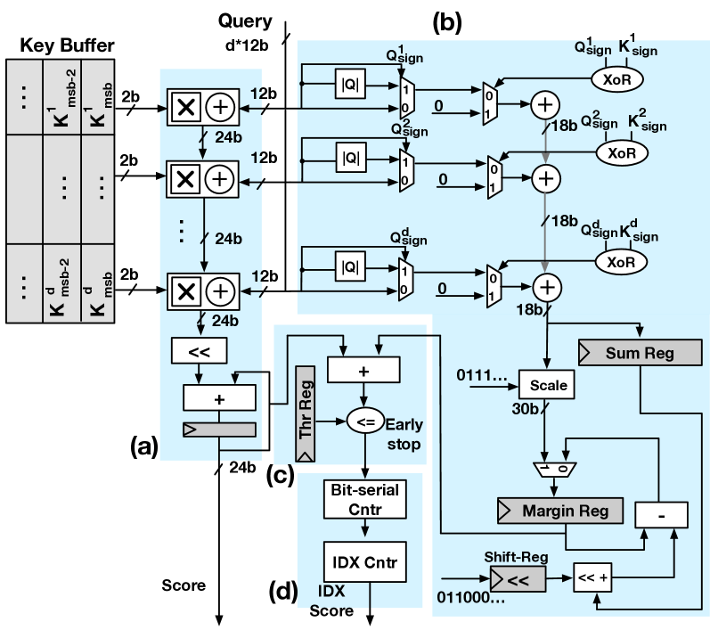
Figure 5. A QK-DPU comprising (a) bit-serial dot-product engine, (b) margin calculation logic, (c) thresholding module, and (d) score index counter.

As discussed in Section 3.2 and Figure 3, to detect whether a current $Score$ needs to be pruned and corresponding computations be terminated, QK-DPU dynamically calculates a conservative upper-bound margin ($\mathcal{M}$) and adds it with the current dot-product partial sum ($\mathcal{P}$) to compare it with the layer threshold ($\mathcal{T}h$). Figure 5-(b) and (c) show the details of hardware realization for margin calculation and thresholding logic, respectively. To calculate the margin according to Table in Figure 3, the margin calculation module first detects the $\mathcal{Q}$ and $\mathcal{K}$ pairs in the dot-product that yield positive product. To do so, during the processing of $\mathcal{K}$’s MSBs, the sign bits of $\mathcal{Q}$s and $\mathcal{K}$s are XORed. Only if the result is positive (XOR = 0), the absolute values of the corresponding $\mathcal{Q}$ are summed up to calculate the margin (e.g., resulting in $(9+5)$ in the Table of Figure 3). The summation result is stored in a Sum Register. Then, it is scaled by the fixed number, largest positive value (e.g. 0111…), which corresponds to $(2^{-1}+2^{-2}+2^{-3}+...)$ in Figure 3, storing $(9+5)(2^{-1}+2^{-2}+2^{-3}+...)$ in the margin register. The margin needs to be calculated dynamically for each bit position during bit-serial execution (such as $\mathcal{M}$ changing in each row of the Table in Figure 3). This is enabled by subtracting the shifted version of Sum Register value from the current margin in the margin register, e.g., $(9+5)(2^{-1}+2^{-2}+2^{-3}+...)-(9+5)(2^{-1})=(9+5)(2^{-2}+2^{-3}+...)$ in the second row of the Table in Figure 3. This operation is iterated every bit position to generate the values in the subsequent rows of the Table in Figure 3. Note that, the margin calculation is a scalar computation (mostly shift and subtraction), which is amortized over the $d=64$ dimension vector processing, incurring virtually no overhead. After each cycle of the bit-serial operation, the thresholding module (Figure 5-(c)) adds the updated partial sum with the current margin and compares it with the layer threshold $\mathcal{T}h$ to determine the continuation of the dot-product or its termination for pruning of the current $Score$.

Final score index calculation. The QK-DPU calculates the indices of the unpruned $Score$s using a set of two counters, as shown in Figure 5-(d). First, Bit-serial Cntr increments with the number of bits processed by the QK-DPU and gets reset whenever it reaches its maximum (i.e. 6 (= 12bit/$\mathcal{B}$)) for processing all bits for unpruned $Score$s) or the Early stop flag is asserted. Second, the value of IDX Cntr shows the position of the current $Score$ in the vector and increments whenever the Bit-serial Cntr gets reset, ending the computation of that $Score$. Finally, if the IDX Cntr increments and the Early stop flag is low, the QK-DPU pushes the content of this counter to IDX FIFO, because it means that the corresponding $Score$ is not pruned and will be used for further processing in the V-PU.

4.3. Back-End Value Processing

As shown in Figure 4-(b), the LeOPArd tile’s back-end stage, V-PU, consumes the unpruned $Score$s and executes the Softmax operation, followed by multiplication with $\mathcal{V}$ vectors and finally storing the results to an Output-FIFO. Whenever the Score-FIFO is not empty, the V-PU starts the Softmax operation ($e^{x}$ and accumulation) to calculate the probabilities. We implemented the Softmax module of V-PU similarly to the Look-Up-Table (LUT)-based methodology in $A^{3}$ (Ham et al., 2020). Whenever the output probability is produced, the V-PU uses the indices of the unpruned $Score$s to read the corresponding $\mathcal{V}$ vector. Finally, the $\mathcal{V}$ vector is weighted by the output of the Softmax module with a 1-D array of MAC units. The elements of $\mathcal{V}$ vector are distributed and the probabilities are shared across the MAC units, similar to a 1-D systolic array. With such design, the V-PU consumes the $Score$s sequentially to complete the weighted-sum of $\mathcal{V}$ vectors, and accumulates the partial results over multiple cycles while only accessing the unpruned $\mathcal{V}$ vectors. As such, it rightfully leverages the provided pruning by the front-end stage and eliminates the inconsequential computations.

5. Evaluation

5.1. Methodology

Workloads. We evaluate LeOPArd on various NLP and Vision models: BERT-Base (BERT-B) (Kenton and Toutanova, 2019), BERT-Large (BERT-L) (Kenton and Toutanova, 2019), MemN2N (Sukhbaatar et al., 2015), ALBERT-XX-Large (ALBERT-XX-L) (Lan et al., 2019), GPT-2-Large (GPT-2-L) (Radford et al., 2019), and ViT-Base (ViT-B) (Dosovitskiy et al., 2021). To evaluate these models, we use five different datasets: (1) Facebook bAbI, which includes 20 different tasks (Weston et al., 2015) for MemN2N, (2) General Language Understanding Evaluation (GLUE) with nine different tasks (Wang et al., 2018) for BERT models, (3) Stanford Question Answering Dataset (SQUAD) (Rajpurkar et al., 2016) with a single task for BERT models and ALBERT-XX-L, (4) WikiText-2 (wik, 2021) for GPT-2-L, and (5) CIFAR-10 (Krizhevsky and Hinton, 2009) for ViT. The dimension ($d$) of $\mathcal{Q}$, $\mathcal{K}$, and $\mathcal{V}$ vectors for all the workloads is 64 except MemN2N with bAbI dataset, which is 20. The sequence length is 50 for MemN2N with bAbI whereas 512 and 384 for BERT and ALBERT-XX-L models with GLUE and SQUAD datasets, respectively. Finally, the sequence length for GPT-2 with WiKiText-2 is 1280.

Table 1. Microarchitectural configurations of a LeOPArd tile.

Hardware modules	Configurations
QK-PU	6 / 8 QK-DPU (=$N_{\mathrm{QK}}$), each 64 (=$\mathcal{D}$) tap 12$\times$2 bit-serial
Key Buffer	48KB in total (= 8KB$\times$6 / 6KB$\times$8 banks), 128-bit port per bank
V-PU	Single 1-D 64 (=$\mathcal{D}$) way 16$\times$16-bit MAC array
Value Buffer	64KB (= 8KB $\times$ 8 banks), 128-bit port per bank
Softmax	24-bit input, 16-bit output, LUT: 1 KB
Score and IDX FIFOs	24-bit $\times$ 512 depth for Score, 8-bit $\times$ 512 depth for IDX

Fine-tuning details. We use the baseline model checkpoints from HuggingFace (Wolf et al., 2019) with PyTorch v1.10 (Paszke et al., 2019) and fine-tune the models on an Nvidia RTX 3090, except for GPT-2-Large, for which we use an Nvidia A100. For default task-level training, we use the Adam optimizer with default parameters and the learning rate of $[2,3]\times{}e^{-5}$ (same as baseline). To obtain the layer-specific threshold values, we perform an additional pruning-aware fine-tuning step for one to five more epochs to learn the optimal values while maintaining the baseline model accuracy. For this step, we use the learning rate of $1e^{-2}$ for $\mathcal{T}h$ ($5e^{-6}$ for the other parameters), as training for the $\mathcal{T}h$ is generally slower and a higher learning rate facilitates convergence. To leverage faster fixed-point execution, we perform a final post-training quantization step with 12 bits for inputs in QK-PU hardware block and 16 bits for V-PU block similarly to (Wang et al., 2021).

Hardware design details. Table 1 lists the microarchitectural parameters of a single LeOPArd tile for two studied configurations: (1) A LeOPArd tile with six and (2) eight QK-DPUs that share a single 1-D MAC array in V-PU. The number of QK-DPUs is set such that the compute utilization for front-end and back-end units is balanced, while considering the pruning and bit-level early-termination rates across all the workloads. We synthesised and performed Placement-and-Route (P&R) for our designs with two tiles. The on-chip memory sizes for $\mathcal{K}$ and $\mathcal{V}$ are designed to store up to 512 sequences for a single head in a layer for both configurations.

Accelerator synthesis and simulations. We use Cadence Genus 19.1 (Cadence, 2021a) and Cadence Innovus 19.1 (Cadence, 2021b) to perform logic synthesis, floorplan, and P&R for the LeOPArd accelerator. We use TSMC 65 nm GP (General Purpose) standard cell library for the synthesis and layout generation of the digital logic blocks. These digital blocks are rigorously generated to meet the target frequency of 800MHz in consideration of all the CMOS corner variations and temperature conditions from $-40^{\circ}$ to $125^{\circ}\mathrm{C}$. For the SRAM on-chip memory blocks, we use Memory Compiler with ARM High density 65 nm GP 6-transistor based single-port SRAM version r0p0 (ARM, 2021).

We also develop a simulator to obtain the total cycle counts and number of accesses to memories for both LeOPArd and baseline accelerators. The simulator incorporates the pruning rate and the bit-level early-termination statistics for each individual workload. Using these statistics, the simulator evaluates runtime and total energy consumption of the accelerators.

Comparison to baseline architecture. We compare LeOPArd to a conventional baseline design without any of our optimizations (e.g. runtime pruning and bit-level early compute termination). For a fair comparison, we use the same frequency, bitwidths for $\mathcal{Q}\times\mathcal{K}{\color[rgb]{0,0,0}^{T}}$ and $\times\mathcal{V}$, and on-chip memory capacity for all the designs. The baseline design employs a single 12$\times$12-bit QK-DPU as opposed to multiple 12$\times$2-bit-serial ones, while both designs have the same back-end V-PU. As shown in Table 1, we evaluate LeOPArd under two design configurations. The first design with six QK-DPUs, dubbed Area-Efficient LeOPArd (AE-LeOPArd), almost perfectly matches the area of the baseline design (¡ 0.2% overhead) and provides an iso-area comparison setting. The second one with eight QK-DPUs, dubbed Highly-Parallel LeOPArd (HP-LeOPArd), provides an area 15% larger than baseline and delivers a better balance in the compute utilization of the front-end and back-end stages.

Comparison with $A^{3}$ and SpAtten. We also compare LeOPArd with two state-of-the-art attention accelerators, $A^{3}$ (Ham et al., 2020) and SpAtten (Wang et al., 2021), with support for runtime pruning. $A^{3}$ employs token pruning by comparing the Softmax output ($\mathrm{probability}$) to a relative threshold, which is set using a user-defined parameter that adjusts the level of approximation. $A^{3}$ also employs a sorting mechanism to make the pruning decision after processing only a small number of large elements from the sorted $\mathcal{K}$ matrix in the order of magnitude. SpAtten performs cascaded head and token pruning by comparing the Softmax output with a user-defined threshold obtained empirically. There are no raw performance/energy results for individual workloads and simulation infrastructures of the accelerators. Therefore, we follow the comparison methodology of SpAtten (Wang et al., 2021), using throughput (GOPs / s), energy efficiency (GOPs / J), and area efficiency (GOPs / s / mm²) metrics to provide the best comparisons. Both $A^{3}$ and SpAtten are implemented in 40 nm technology. To provide a fair comparison, we scale HP-LeOPArd from 65 nm to 40 nm based on both Dennard scaling (indicated with ^†) and measurement-based scaling rules (Stillmaker and Baas, 2017) (indicated with ^‡). We use a single tile with an area comparable to $A^{3}$ and SpAtten. Moreover, $A^{3}$ implements the $\mathcal{Q}\times\mathcal{K}{\color[rgb]{0,0,0}^{T}}$ using 9 bits as opposed to 12 bits in LeOPArd. As such, we scale the QK-PU of HP-LeOPArd from 12 bits to 9 bits to provide a head-to-head comparison with $A^{3}$.

5.2. Accuracy and Algorithmic Optimization

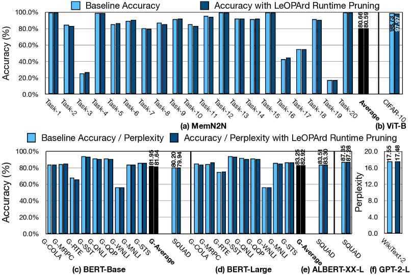
Figure 6. Accuracy before and after pruning-aware fine-tuning (prefix ”G-”: GLUE). We evaluate GPT-2 using perplexity, which favors a lower value.

Impacts on model accuracy. Figure 6 compares the accuracies of the LeOPArd gradient-based on-the-fly pruning method and the baseline models in their vanilla implementation (Wolf et al., 2019), across various tasks of evaluated workloads. On average, across all the evaluated tasks, LeOPArd runtime pruning degrades accuracy by only 0.07% for MemN2N with the bAbi dataset, 0.31% and 0.33% for BERT-B and BERT-L with the GLUE dataset, and 0.26% and 0.21% for BERT-B and BERT-L with the SQUAD dataset. For ALBERT-XX-L with the SQUAD dataset, the LeOPArd runtime pruning leads to only an 0.07% accuracy loss, whereas the degradation for ViT-B with the CIFAR-10 dataset is 0.76%.

In the GPT-2-L model, we use perplexity, which is the key metric for auto regressive language models. Note that perplexity is derived from the model loss, and thus lower perplexity is better. As shown in Figure 6-(f), LeOPArd runtime pruning results in a 0.07 decrease in perplexity. This is achievable because LeOPArd learns the optimal threshold values and co-adjusts them with the weight parameters simultaneously via gradient-based optimization. Figure 6 also illustrates that the LeOPArd pruning-aware fine-tuning pass evenly improves the accuracy for some of the benchmark tasks, with the maximum of 2.2%. However, this also degrades the accuracy for other tasks with the maximum of 2.6%. This accuracy fluctuations are unavoidable due to randomness in deep learning training, but overall the accuracy degradation, averaged across the evaluated benchmarks, converges adequately to a near-zero value ($\leq$ 0.2%). Performing the post-training quantization adds at most only 0.1%, for both the baseline and our pruning-aware fine-tuned models.

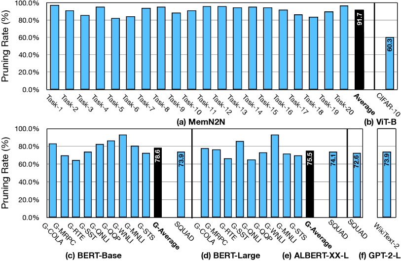
Figure 7. Runtime pruning rate with LeOPArd. (prefix ”G-”: GLUE)

Runtime pruning rate analysis. Figure 7 shows the percentage of total $\mathcal{Q}\times\mathcal{K}{\color[rgb]{0,0,0}^{T}}$ $Score$s that are pruned away by our method using the learned threshold values across various benchmarks. In transformer software implementations, zeros are padded to maintain regular vector length despite the varying sequence length in each workload. The padded zeros are not counted for sparsity contribution in this paper. On average, LeOPArd prunes 91.7% (max. 97.4%) of $Score$s across all the 20 tasks for the MeMN2N model with the bAbI dataset. LeOPArd achieves the average pruning rates of 78.6% (max. 93.2%) and 75.5% (max. 93.0%) for the BERT-B and BERT-L models with the GLUE dataset, while achieving 73.9% and 74.1% with the SQUAD dataset, respectively. Moreover, LeOPArd provides a 72.6% pruning rate for ALBERT-XX-L with the SQUAD dataset, 60.3% for ViT-B with the CIFAR-10 dataset, and 73.9% for GPT-2-L with the WikiText-2 dataset. As the results suggest, LeOPArd can significantly prune out the $Score$s across various tasks, with greater benefits to MeMN2N tasks compared to the BERT ones. We conjecture the lower pruning rates in BERT models are due to the higher probability of correlation between various tokens in the more complex language processing tasks compared to MemN2N.

Table 2. LeOPArd performance comparison under different scenarios with prior work (Ham et al., 2020; Wang et al., 2021).

Metric (unit)	A3-Base	A3-Conserv	SpAtten	HP-LeOPArd	HP-LeOPArd †	HP-LeOPArd ‡	HP-LeOPArd †∗	HP-LeOPArd ‡∗
Process (nm)	40	40	40	65	40	40	40	40
Area (mm2)	2.08	2.08	1.55	3.47	1.31	1.31	1.05	1.05
Key Buffer (KB)	20	20	24	48	24	24	24	24
Value Buffer (KB)	20	20	24	64	24	24	24	24
($\mathcal{Q}$, $\mathcal{K}$)-bits	(9, 9)	(9, 9)	(12, 12)	(12, 12)	(12, 12)	(12, 12)	(9, 9)	(9, 9)
GOPs / s	259.0	518.0	728.4	574.1	932.8	1084.9	1143.9	1330.3
GOPs / J	2354.5	4709.1	772.9	519.3	2224.8	2028.8	3353.8	3058.4
GOPs / s / mm2	124.5	249.0	470.0	165.5	710.4	826.1	1093.8	1272.1

$\dagger$ Dennard scaling trend applied to map on 40 nm process – $\ddagger$ Scaling rule from (Stillmaker and Baas, 2017) applied to map on 40 nm process – *scaled to 9 bit $\mathcal{Q}$, $\mathcal{K}$

As Figure 7 shows, in the case of ALBERT-XX-L with SQUAD, we see more pruning opportunities compared to BERT, presumably because of its larger model architecture with more redundant computations. Similar trend is observed for GPT-2-L. With regard to ViT-B, we see lower pruning compared to NLP tasks, commensurate with prior studies (Chen et al., 2021b). This occurs because information is more local in images compared to texts, and therefore there is less redundancy in the attention layers for vision tasks.

Bit-level early-compute termination. Figure 8 depicts the proposed bit-level early compute termination feature and its relation with the achieved runtime pruning rates. The x-axis shows the number of bits processed sequentially, while the y-axis shows the cumulative achieved pruning rate averaged over all of the datasets’ tasks. Intuitively, as more bits are processed during $Score$ computations, the dynamic margin becomes smaller and thus the pruning rate increases. As shown, as the average number of processed bits increases, the cumulative pruning rate gradually plateaus, indicating saturation. In this scenario, the higher number of bits are only required for fully calculating unpruned $Score$s. We establish that the lower redundancy in model parameters of some transformer models, e.g. BERT-L / ViT-B, hinders higher runtime pruning. Because lower redundancy generally translates to a higher number of average bits calculations, it proportionally diminishes the potential gains from bit-wise early termination. Averaged over pruned $Score$s in bit-serial mode, MemN2N with the bAbi dataset requires 4.5 bits, while BERT-B and BERT-L require 8.3 and 8.0 bits with the GLUE dataset. With the SQUAD dataset, the average number of bits in BERT-B and BERT-L are 7.6 and 9.0 bits, whereas ALBERT-XX-L maintains 8.0 bits. The average number of bits in GPT-2-L and ViT attain 7.6 bits and 8.5 bits, respectively. This devised early-termination mechanism significantly reduces the computations of the $\mathcal{Q}\times\mathcal{K}{\color[rgb]{0,0,0}^{T}}$.

5.3. Accelerator Performance Results

Performance and energy comparison to baseline. Figure 9 shows the speedup improvements delivered by LeOPArd compared to the baseline design, across all the 43 studied tasks. In this comparison, we consider the total execution runtime for all attention layers of the models. On average across all tasks, AE-LeOPArd and HP-LeOPArd provide 1.9$\times$ and 2.4$\times$ speedup over the baseline, respectively. These improvements stem from both LeOPArd runtime pruning that reduces operations on the back-end unit (e.g., Softmax and $\times\mathcal{V}$) and bit-level early compute termination that saves cycles on $\mathcal{Q}\times\mathcal{K}{\color[rgb]{0,0,0}^{T}}$ computations for pruned $Score$s. Across the workloads, LeOPArd delivers higher speedups for MemN2N compared to the other benchmarks. We attribute these improvements to the higher pruning rate and consequently more bit-level termination opportunities in this model’s tasks. Among all the tasks, MemN2N-Task-1 enjoys the maximal speedup (3.8$\times$ for AE-LeOPArd and 5.1$\times$ for HP-LeOPArd) while ViT-B gains the minimal improvements (1.1$\times$ for both AE-LeOPArd and HP-LeOPArd).

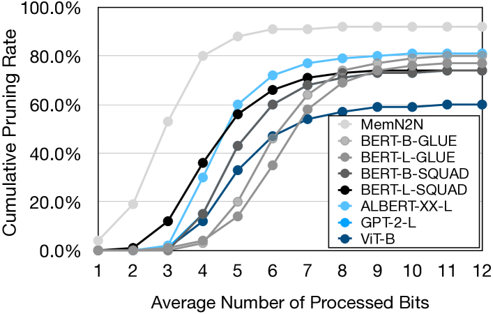
Figure 8. Cumulative pruning rate with respect to the number of bits processed during bit-serial early termination. Each line obtained by averaging across all the pruning rates per task.

The benefits are more pronounced for HP-LeOPArd because it deploys more QK-DPUs, which both improves the performance of the front-end Q-PU unit, and delivers more inputs ($Score$s) to the back-end stage. The latter generally increases the back-end utilization.

Figure 9. Speedup comparison to baseline design for AE-LeOPArd and HP-LeOPArd (prefix ”G-”: GLUE dataset).

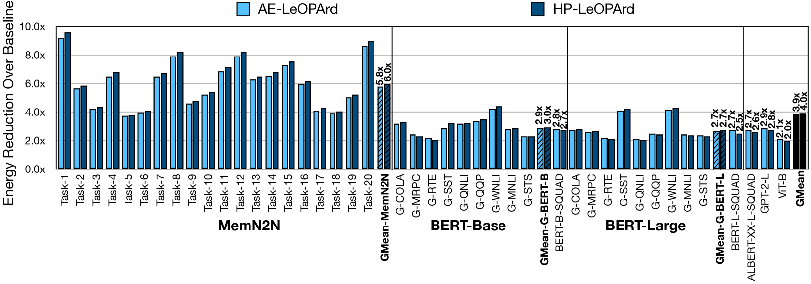
Figure 10. Total energy reduction for AE-LeOPArd and HP-LeOPArd compared to baseline (prefix ”G-”: GLUE dataset).

Figure 10 compares the energy reduction (including compute and on-chip memory accesses) achieved by LeOPArd to the baseline. On average, LeOPArd reduces total energy consumption by a factor of 3.9$\times$ for AE-LeOPArd and 4.0$\times$ for HP-LeOPArd, across all the studied tasks. Similarly to the speedup comparisons, MemN2N enjoys a greater energy reduction than the other benchmarks due to the higher pruning rate and therefore faster bit-level compute terminations. Across all tasks, the energy reduction is the greatest for MemN2N-Task-1 (9.2$\times$ for AE-LeOPArd and 9.6$\times$ for HP-LeOPArd) and ViT-B achieves the lowest savings ($\approx$ 2.0$\times$ for AE-LeOPArd and HP-LeOPArd). The impact of LeOPArd on energy exceeds that on speedup, because runtime pruning and bit-level early termination reduce computation energy (contributing to both energy savings and speedup) and memory accesses (only contributing to energy savings). The energy reductions for both AE-LeOPArd and HP-LeOPArd are not substantially different. Because the additional QK-DPUs in HP-LeOPArd increase both power and performance, total energy consumption remains similar.

Analysis of energy savings breakdown. Figure 11 analyzes the breakdown of total energy consumption across five microarchitectural components: (1) $\mathcal{Q}\times\mathcal{K}{\color[rgb]{0,0,0}^{T}}$ computations, (2) $\mathcal{K}$ buffer memory access, (3) Softmax, (4) $\times\mathcal{V}$ computations, and (5) value buffer memory access. We report the average breakdown across all tasks for each workload. Additionally, Figure 11 illustrates the contribution of LeOPArd’s two main optimizations: (1) runtime pruning and (2) early compute termination through bit-serial execution to the overall energy savings in AE-LeOPArd. We normalize the energy breakdowns to a baseline, which does not utilize any of the LeOPArd’s optimizations. In the baseline, $\times\mathcal{V}$ computations and value buffer memory accesses proportionally consume the highest energy due to the lack of runtime pruning; ergo, higher average number of bits in $\mathcal{Q}\times\mathcal{K}^{T}$. Recall that the LeOPArd’s back-end unit encloses Softmax, $\times\mathcal{V}$, and its associated buffer accesses. As the results show, this unit consumes more than 65$\%$ of the total energy in the baseline design. LeOPArd’s runtime pruning enables skipping computations and memory accesses for inconsequential $Score$s during the back-end processing, delivering 1.7$\times$ (ViT-B) to 2.5$\times$ (MemN2N) energy savings. For these tasks, the bit-serial execution in LeOPArd along with its early termination brings further energy savings of 1.3$\times$ (ViT-B) to 2.3$\times$ (MemN2N) on top of runtime pruning. These additional benefits arise from avoiding the inconsequential bit computations in $\mathcal{Q}\times\mathcal{K}$ and their associated $\mathcal{K}$ buffer accesses.

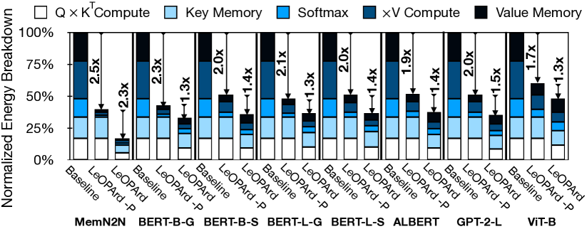
Figure 11. Normalized LeOPArd’s average energy breakdown and the contribution of runtime pruning and bit-level early termination in energy saving (LeOPArd-P: with only pruning, and LeOPArd: pruning $+$ bit-serial early termination) across one transformer head.

Comparison with $A^{3}$ and SpAtten.  Table 2 compares the characteristics and performance of HP-LeOPArd and its scaled versions with $A^{3}$ and SpAtten. Compared to SpAtten, HP-LeOPArd^† (HP-LeOPArd^‡) delivers 3$\times$ (2.6$\times$) improvements in GOPs / J and 1.5$\times$ (1.7 $\times$) improvements in GOPs / s / mm², while both designs have virtually no model accuracy degradation. These benefits are attributed to the LeOPArd’s higher pruning rate and to the bit-level early compute termination. For comparison with $A^{3}$, we evaluate HP-LeOPArd^†∗ (HP-LeOPArd^‡∗), which are scaled to 40 nm and deploy 9-bit arithmetic for $\mathcal{Q}\times\mathcal{K}{\color[rgb]{0,0,0}^{T}}$. A³-Conservative deploys heuristic approximation to minimize accuracy degradation on top of A³-Base, which does not use approximation. HP-LeOPArd^†∗ (HP-LeOPArd^‡∗) achieves 1.4$\times$ (1.3$\times$) higher energy efficiency (in GOPs / J) and 8.8$\times$ (10.2$\times$) area efficiency (in GOPs / s / mm²) than A³-base. HP-LeOPArd^†∗ (HP-LeOPArd^‡∗) also provides 4.4$\times$ (5.1$\times$) improvements in terms of GOPs / s / mm² compared to A³-Conservative. Although A³-Conservative provides 29% and 35% higher energy efficiency compared to HP-LeOPArd^†∗ and HP-LeOPArd^‡∗, respectively, this comes at the cost of visible accuracy degradation, e.g., 1.0% for MemN2N and 1.3% for BERT-Base with the SQUAD dataset as reported in (Ham et al., 2020). On the other hand, LeOPArd’s carefully crafted gradient-based training balances pruning rate and model accuracy, providing accuracy degradation of only 0.06% and 0.26% for the aforementioned models and datasets without manual configurations for heuristic parameters.

LeOPArd accelerator layout area details. Figure 12(a) shows the layout of LeOPArd architecture, which occupies $2.3\times 2.8~{}\mathrm{mm^{2}}$, including two tiles. The layouts are generated by meeting the design rule check in a 65 nm process and targeting 65-75% physical density, commonly used for the routing convenience and tape-out yield. Figure 12-(b) reports the area breakdown, where QK-DPU takes the largest proportion as we employ $N_{\mathrm{QK}}$ QK-DPU in consideration of the high pruning rate. This leads to 56% area occupied by the front-end unit, which includes QK-DPU and $\mathcal{K}$ buffer. The on-chip memory for $\mathcal{K}$ and $\mathcal{V}$ occupies 34% of the layout area.

5.4. Architecture Design Space Exploration

QK-PU parallelism degree. As discussed in Section 4.1, the number of QK-DPUs ($N_{\mathrm{QK}}$) within one QK-PU exhibits a trade-off space in designing the LeOPArd accelerator.

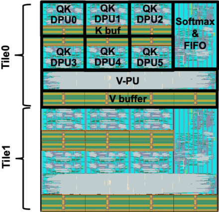
(a)

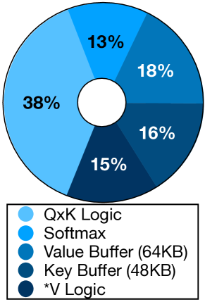
(b)

Figure 12. AE-LeOPArd: (a) layout ($2.3\times 2.8~{}\mathrm{mm^{2}}$) and (b) area breakdown.

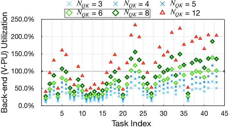
Figure 13. Back-end V-PU utilization over the QK-PU parallelism ($N_{\mathrm{QK}}$). $N_{QK}=6$ and $N_{QK}=8$ form the favorable configurations in terms of back-end utilization in AE-LeOPArd and HP-LeOPArd, respectively.

To find the number of QK-DPUs that balances the utilization of front-end and back-end units, we sweep the $N_{\mathrm{QK}}$ from three to 12 in Figure 13 and report the V-PU utilization across the evaluated tasks. If utilization exceeds 100$\%$ (common when $N_{\mathrm{QK}}=12$), the back-end V-PU is over-subscribed due to the throughput mismatch between V-PU and QK-PU. This mismatch throttles the back-end V-PU and turns into the system bottleneck, frequently stalling the front-end. On the other hand, when $N_{\mathrm{QK}}=3$, the V-PU is chronically under-utilized due to a significant reduction in its number of computations, attributed to front-end runtime pruning mechanism. As marked by dark green diamonds, $N_{\mathrm{QK}}=8$ adequately balances the V-PU utilization and the number of front-end unit stalls. Thus, we favor this configuration for HP-LeOPArd. The second best configuration to balance front- and back-end utilization is $N_{\mathrm{QK}}=6$ (marked by light green diamonds). As such, we choose this configuration for AE-LeOPArd, which matches the baseline chip area usage.

Bit-serial processing granularity.  Figure 14 illustrates the design space exploration for granularity of the bit-serial execution in QK-DPU ($\mathcal{B}$). This bit-level granularity creates a trade-off space, where decreasing the $\mathcal{B}$ stores intermediate results at the end of each bit processing cycle more frequently (escalating the energy). At the same time, increasing $\mathcal{B}$ curtails the performance of early compute termination due to lower resolution in stopping the computations. To find the optimal point, we sweep the $\mathcal{B}$ for values of 1, 2, 4, and 12 bits and measure the average consumed energy and its breakdown ($\mathcal{Q}\times\mathcal{K}{\color[rgb]{0,0,0}^{T}}$ logic and key buffer accesses) per one output $Score$. All the numbers are normalized to 12-bit processing that does not employ any bit-serial execution. Figure 14 depicts this analysis for MemN2N tasks (results for other models are similar) and reports the average across all tasks. As shown, 2-bit-serial execution strikes the right balance between energy consumption of the bit-serial computations and the resolution of bit-level early compute termination.

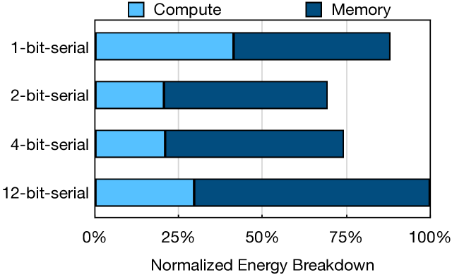
Figure 14. Design space exploration for the resolution ($\mathcal{B}$) of bit-serial execution with respect to normalized average QK-DPU energy per $Score$.

6. Related Work

In contrast with prior work, LeOPArd explores a distinct design space for accelerating attention models through gradient-based learned runtime pruning. This tight integration of pruning and training enables LeOPArd to reduce the computation cost with virtually zero accuracy degradation across a range of language and vision transformer models. Building on these algorithmic insights, we devise a bit-serial execution strategy that conservatively terminates the computations as early as possible. Below, we cover the most relevant work and position our paper with respect to it.

Hardware-algorithm co-design for attention models. Several algorithmic optimizations co-designed with hardware acceleration were proposed for efficient execution of attention models (Ham et al., 2021; Wang et al., 2021; Lu et al., 2021; Tambe et al., 2021; Stevens et al., 2021; Ham et al., 2020; Park et al., 2020; Zadeh et al., 2020). $A^{3}$ has proposed an approximation method with a hardware accelerator to prune out the ineffectual computations in attention. This method searches effective data during the $query\times key$ operation in addition to another approximation mechanism after score calculation. SpAtten (Wang et al., 2021) prunes the ineffectual input tokens and heads, in addition to progressive quantization during computations at runtime, to improve the performance and memory bandwidth. We provide a head-to-head comparison to these works in Section 5.3. ELSA (Ham et al., 2021) aims to address the costly candidate search process of $A^{3}$ and incorporates a user-defined ”confidence-level” parameter to find the optimal thresholds from training statistics. EdgeBERT (Tambe et al., 2021) leverages entropy-based early exiting technique to predict the minimal number of transformer layers that need to be executed, while the rest can be skipped. Other works aim to address the computational cost of self-attention via sparse matrix operation (Park et al., 2020; Lu et al., 2021; Chen et al., 2021a), quantization (Zadeh et al., 2020), and Softmax approximation (Stevens et al., 2021). Moreover, none of these prior designs explored bit-level early compute termination.

Algorithmic optimizations for transformer acceleration. Another line of prior inquiry proposes only algorithmic optimizations to provide sparsity in computing attention models. Proposals in (Roy et al., 2021; Beltagy et al., 2020; Ye et al., 2021; Kitaev et al., 2020; Qiu et al., 2019; Ye et al., 2019; Child et al., 2019; Michel et al., 2019; Wang et al., 2019; Wen et al., 2017) offer static sparsity in the attention layers to reduce its significant computational cost. Other work (Zhao et al., 2019; Correia et al., 2019; Cui et al., 2019) provides dynamic sparsity based on the input samples, yet still requires full computation of the $\mathcal{Q}\mathcal{\times}\mathcal{K}{\color[rgb]{0,0,0}^{T}}$. Our proposal fundamentally differs from this prior seminal work, because it formulates the problem of pruning threshold finding as a regularizer to methodically co-optimize with the weight parameters of the models, without approximation. Additionally, LeOPArd provides architectural support to stop the attention computations as early as possible during runtime.

Early compute-termination in DNNs. Prior work (Shomron et al., 2020; Aklaghi et al., 2018; Lee et al., 2018a; Lin et al., 2017) has proposed techniques to early terminate the computations of convolution layers by leveraging the zero production feature of ReLU for negative numbers. In contrast, this work focuses on early termination of a fundamentally different operator, attention in transformers, and provides unique mechanisms to enable that. Moreover, the prior works consider zero as a fixed threshold in their methods, but LeOPArd formulates the thresholds as a regularizer and finds layer-wise values through gradient descent optimization to preserve the accuracy of the models.

DNN acceleration. A large swath of work (Yazdanbakhsh et al., 2021; Ghodrati et al., 2020b, c; Qin et al., 2020; Ghodrati et al., 2020a; Delmas Lascorz et al., 2019; Samragh et al., 2019; Ryu et al., 2019; Sharify et al., 2019; Hussain et al., 2019; Gao et al., 2019; Chen et al., 2019; Shao et al., 2019; Kwon et al., 2019, 2018; Fowers et al., 2018; Sharma et al., 2018; Yazdanbakhsh et al., 2018a; Rouhani et al., 2018; Lee et al., 2018b; Yazdanbakhsh et al., 2018b; Sharify et al., 2018; Eckert et al., 2018; Parashar et al., 2017; Albericio et al., 2017; Song et al., 2017; Gao et al., 2017; Jouppi et al., 2017; Han et al., 2016; Judd et al., 2016; Reagen et al., 2016; Kim et al., 2016; Shafiee et al., 2016; Chi et al., 2016; Zhang et al., 2016; Albericio et al., 2016; Liu et al., 2016; Chen et al., 2016; Sharma et al., 2016; Yazdanbakhsh et al., 2015; St. Amant et al., 2014; Chen et al., 2014) is dedicated to accelerating DNNs. Although inspiring, these designs do not deal with the challenges unique to the attention mechanisms of transformers, as opposed to this work.

7. Conclusion

Transformers through the self-attention mechanism have triggered an exciting new wave in machine learning, notably in Natural Language Processing (NLP). The self-attention mechanism computes pairwise correlations among all the words in a subtext. This task is both compute and memory intensive and has become one of the key challenges in realizing the full potential of attention models. One opportunity to slash the overheads of the self-attention mechanism is to limit the correlation computations to a few high score words and computationally prune the inconsequential scores at runtime through a thresholding mechanism. This work exclusively formulated the threshold finding as a gradient-based optimization problem. This formulation strikes a formal and analytical balance between model accuracy and computation reduction. To maximize the performance gains from thresholding, this paper also devised a bit-serial architecture to enable an early-termination atop pruning with no repercussions to model accuracy. These techniques synergistically yield significant benefits both in terms of speedup and energy savings across various transformer-based models on a range of NLP and vision tasks. The application of the proposed mathematical formulation of identifying threshold values and its cohesive integration into the training loss is broad and can potentially be adopted across a wide range of compute reduction techniques.

- (1)
- ai_(2021) 2021. AI Winter. https://en.wikipedia.org/wiki/AI˙winter. Accessed: 2021-11-08.
- wik (2021) 2021. The WikiText Long Term Dependency Language Modeling Dataset. https://blog.salesforceairesearch.com/the-wikitext-long-term-dependency-language-modeling-dataset/. Accessed: 2021-11-08.
- tur (2021) 2021. Turing Test. https://en.wikipedia.org/wiki/Turing˙test. Accessed: 2021-11-08.
- Aklaghi et al. (2018) Vahide Aklaghi, Amir Yazdanbakhsh, Kambiz Samadi, Hadi Esmaeilzadeh, and Rajesh K. Gupta. 2018. SnaPEA: Predictive Early Activation for Reducing Computation in Deep Convolutional Neural Networks. In ISCA.
- Albericio et al. (2017) Jorge Albericio, Alberto Delmás, Patrick Judd, Sayeh Sharify, Gerard O’Leary, Roman Genov, and Andreas Moshovos. 2017. Bit-Pragmatic Deep Neural Network Computing. In MICRO.
- Albericio et al. (2016) Jorge Albericio, Patrick Judd, Tayler Hetherington, Tor Aamodt, Natalie Enright Jerger, and Andreas Moshovos. 2016. Cnvlutin: Ineffectual-Neuron-Free Deep Neural Network Computing. In ISCA.
- ARM (2021) ARM. 2021. Artisan Memory Compilers. https://developer.arm.com/ip-products/physical-ip/embedded-memory. Accessed: 2021-11-08.
- Azarian et al. (2020) Kambiz Azarian, Yash Bhalgat, Jinwon Lee, and Tijmen Blankevoort. 2020. Learned Threshold Pruning. arXiv preprint arXiv:2003.00075.
- Beltagy et al. (2020) Iz Beltagy, Matthew E Peters, and Arman Cohan. 2020. Longformer: The Long-Document Transformer. arXiv preprint arXiv:2004.05150.
- Brown et al. (2020) Tom Brown, Benjamin Mann, Nick Ryder, Melanie Subbiah, Jared D Kaplan, Prafulla Dhariwal, Arvind Neelakantan, Pranav Shyam, Girish Sastry, Amanda Askell, et al. 2020. Language Models are Few-shot Learners. NeurIPS.
- Cadence (2021a) Cadence. 2021a. Genus Synthesis Solution. https://www.cadence.com/en˙US/home/tools/digital-design-and-signoff/synthesis/genus-synthesis-solution.html. Accessed: 2021-11-08.
- Cadence (2021b) Cadence. 2021b. Innovus Implementation System. https://www.cadence.com/en˙US/home/tools/digital-design-and-signoff/soc-implementation-and-floorplanning/innovus-implementation-system.html. Accessed: 2021-11-08.
- Chen et al. (2021a) Tianlong Chen, Yu Cheng, Zhe Gan, Lu Yuan, Lei Zhang, and Zhangyang Wang. 2021a. Chasing Sparsity in Vision Transformers: An End-to-End Exploration. NeurIPS.
- Chen et al. (2021b) Tianlong Chen, Yu Cheng, Zhe Gan, Lu Yuan, Lei Zhang, and Zhangyang Wang. 2021b. Chasing Sparsity in Vision Transformers:An End-to-End Exploration. arXiv:2106.04533
- Chen et al. (2014) Yunji Chen, Tao Luo, Shaoli Liu, Shijin Zhang, Liqiang He, Jia Wang, Ling Li, Tianshi Chen, Zhiwei Xu, Ninghui Sun, et al. 2014. DaDianNao: A Machine-Learning Supercomputer. In MICRO.
- Chen et al. (2016) Yu-Hsin Chen, Joel Emer, and Vivienne Sze. 2016. Eyeriss: A Spatial Architecture for Energy-Efficient Dataflow for Convolutional Neural Networks. In ISCA.
- Chen et al. (2019) Yu-Hsin Chen, Tien-Ju Yang, Joel Emer, and Vivienne Sze. 2019. Eyeriss v2: A Flexible Accelerator for Emerging Deep Neural Networks on Mobile Devices. JETCAS (2019).
- Chi et al. (2016) Ping Chi, Shuangchen Li, Cong Xu, Tao Zhang, Jishen Zhao, Yongpan Liu, Yu Wang, and Yuan Xie. 2016. Prime: A Novel Processing-in-Memory Architecture for Neural Network Computation in ReRAM-based Main Memory. In ISCA.
- Child et al. (2019) Rewon Child, Scott Gray, Alec Radford, and Ilya Sutskever. 2019. Generating Long Sequences with Sparse Transformers. arXiv preprint arXiv:1904.10509.
- Choromanski et al. (2020) Krzysztof Choromanski, Valerii Likhosherstov, David Dohan, Xingyou Song, Andreea Gane, Tamas Sarlos, Peter Hawkins, Jared Davis, Afroz Mohiuddin, Lukasz Kaiser, et al. 2020. Rethinking Attention with Performers. arXiv preprint arXiv:2009.14794.
- Correia et al. (2019) Gonçalo M Correia, Vlad Niculae, and André FT Martins. 2019. Adaptively sparse transformers. arXiv preprint arXiv:1909.00015 (2019).
- Cui et al. (2019) Baiyun Cui, Yingming Li, Ming Chen, and Zhongfei Zhang. 2019. Fine-Tune BERT with Sparse Self-Attention Mechanism. In EMNLP-IJCNLP.
- Dai et al. (2019) Zihang Dai, Zhilin Yang, Yiming Yang, Jaime Carbonell, Quoc V Le, and Ruslan Salakhutdinov. 2019. Transformer-XL: Attentive Language Models Beyond a Fixed-length Context. arXiv preprint arXiv:1901.02860.
- Delmas Lascorz et al. (2019) Alberto Delmas Lascorz, Patrick Judd, Dylan Malone Stuart, Zissis Poulos, Mostafa Mahmoud, Sayeh Sharify, Milos Nikolic, Kevin Siu, and Andreas Moshovos. 2019. Bit-Tactical: A Software/Hardware Approach to Exploiting Value and Bit Sparsity in Neural Networks. In ASPLOS.
- Dosovitskiy et al. (2021) Alexey Dosovitskiy, Lucas Beyer, Alexander Kolesnikov, Dirk Weissenborn, Xiaohua Zhai, Thomas Unterthiner, Mostafa Dehghani, Matthias Minderer, Georg Heigold, Sylvain Gelly, Jakob Uszkoreit, and Neil Houlsby. 2021. An Image is Worth 16x16 Words: Transformers for Image Recognition at Scale. In ICLR.
- Eckert et al. (2018) Charles Eckert, Xiaowei Wang, Jingcheng Wang, Arun Subramaniyan, Ravi Iyer, Dennis Sylvester, David Blaaauw, and Reetuparna Das. 2018. Neural Cache: Bit-Serial In-Cache Acceleration of Deep Neural Networks. In ISCA.
- Fowers et al. (2018) Jeremy Fowers, Kalin Ovtcharov, Michael Papamichael, Todd Massengill, Ming Liu, Daniel Lo, Shlomi Alkalay, Michael Haselman, Logan Adams, Mahdi Ghandi, et al. 2018. A Configurable Cloud-Scale DNN Processor for Real-Time AI. In ISCA.
- Gale et al. (2019) Trevor Gale, Erich Elsen, and Sara Hooker. 2019. The State of Sparsity in Deep Neural Networks. arXiv preprint arXiv:1902.09574.
- Gao et al. (2017) Mingyu Gao, Jing Pu, Xuan Yang, Mark Horowitz, and Christos Kozyrakis. 2017. TETRIS: Scalable and Efficient Neural Network Acceleration with 3D Memory. In ASPLOS.
- Gao et al. (2019) Mingyu Gao, Xuan Yang, Jing Pu, Mark Horowitz, and Christos Kozyrakis. 2019. Tangram: Optimized Coarse-Grained Dataflow for Scalable NN Accelerators. In ASPLOS.
- Ghodrati et al. (2020a) Soroush Ghodrati, Byung Hoon Ahn, Joon Kyung Kim, Sean Kinzer, Brahmendra Reddy Yatham, Navateja Alla, Hardik Sharma, Mohammad Alian, Eiman Ebrahimi, Nam Sung Kim, et al. 2020a. Planaria: Dynamic Architecture Fission for Spatial Multi-Tenant Acceleration of Deep Neural Networks. In MICRO.
- Ghodrati et al. (2020b) Soroush Ghodrati, Hardik Sharma, Sean Kinzer, Amir Yazdanbakhsh, Jongse Park, Nam Sung Kim, Doug Burger, and Hadi Esmaeilzadeh. 2020b. Mixed-Signal Charge-Domain Acceleration of Deep Neural networks through Interleaved Bit-Partitioned Arithmetic. In PACT.
- Ghodrati et al. (2020c) Soroush Ghodrati, Hardik Sharma, Cliff Young, Nam Sung Kim, and Hadi Esmaeilzadeh. 2020c. Bit-Parallel Vector Composability for Neural Acceleration. In DAC.
- Ham et al. (2020) Tae Jun Ham, Sung Jun Jung, Seonghak Kim, Young H Oh, Yeonhong Park, Yoonho Song, Jung-Hun Park, Sanghee Lee, Kyoung Park, Jae W Lee, et al. 2020. A^3: Accelerating Attention Mechanisms in Neural Networks with Approximation. In HPCA.
- Ham et al. (2021) Tae Jun Ham, Yejin Lee, Seong Hoon Seo, Soosung Kim, Hyunji Choi, Sung Jun Jung, and Jae W Lee. 2021. ELSA: Hardware-Software Co-design for Efficient, Lightweight Self-Attention Mechanism in Neural Networks. In ISCA.
- Han et al. (2016) Song Han, Xingyu Liu, Huizi Mao, Jing Pu, Ardavan Pedram, Mark A Horowitz, and William J Dally. 2016. EIE: Efficient Inference Engine on Compressed Deep Neural Network. In ISCA.
- Hussain et al. (2019) Shehzeen Hussain, Mojan Javaheripi, Paarth Neekhara, Ryan Kastner, and Farinaz Koushanfar. 2019. FastWave: Accelerating Autoregressive Convolutional Neural Networks on FPGA. In ICCAD.
- Jouppi et al. (2017) Norman P Jouppi, Cliff Young, Nishant Patil, David Patterson, Gaurav Agrawal, Raminder Bajwa, Sarah Bates, Suresh Bhatia, Nan Boden, Al Borchers, et al. 2017. In-Datacenter Performance Analysis of a Tensor Processing Unit. In ISCA.
- Judd et al. (2016) Patrick Judd, Jorge Albericio, Tayler Hetherington, Tor M Aamodt, and Andreas Moshovos. 2016. Stripes: Bit-serial Deep Neural Network Computing. In MICRO.
- Jumper et al. (2021) John Jumper, Richard Evans, Alexander Pritzel, Tim Green, Michael Figurnov, Olaf Ronneberger, Kathryn Tunyasuvunakool, Russ Bates, Augustin Žídek, Anna Potapenko, et al. 2021. Highly Accurate Protein Structure Prediction with AlphaFold. Nature (2021).
- Kao et al. (2021) Sheng-Chun Kao, Suvinay Subramanian, Gaurav Agrawal, and Tushar Krishna. 2021. An Optimized Dataflow for Mitigating Attention Performance Bottlenecks. arXiv preprint arXiv:2107.06419.
- Katharopoulos et al. (2020) Angelos Katharopoulos, Apoorv Vyas, Nikolaos Pappas, and François Fleuret. 2020. Transformers are RNNs: Fast AutoRegressive Transformers with Linear Attention. In ICML.
- Kenton and Toutanova (2019) Jacob Devlin Ming-Wei Chang Kenton and Lee Kristina Toutanova. 2019. BERT: Pre-training of Deep Bidirectional Transformers for Language Understanding. In NAACL-HLT.
- Kim et al. (2016) Duckhwan Kim, Jaeha Kung, Sek Chai, Sudhakar Yalamanchili, and Saibal Mukhopadhyay. 2016. Neurocube: A Programmable Digital Neuromorphic Architecture with High-Density 3D Memory. In ISCA.
- Kingma and Ba (2014) Diederik P Kingma and Jimmy Ba. 2014. Adam: A Method for Stochastic Optimization. arXiv preprint arXiv:1412.6980.
- Kitaev et al. (2020) Nikita Kitaev, Łukasz Kaiser, and Anselm Levskaya. 2020. Reformer: The Efficient Transformer. arXiv preprint arXiv:2001.04451.
- Kolen and Kremer (2001) John F. Kolen and Stefan C. Kremer. 2001. Gradient Flow in Recurrent Nets: The Difficulty of Learning LongTerm Dependencies.
- Krizhevsky and Hinton (2009) Alex Krizhevsky and Geoffrey Hinton. 2009. Learning Multiple Layers of Features from Tiny Images. Computer Science Department, University of Toronto, Tech. Rep (2009).
- Krogh and Hertz (1992) Anders Krogh and John A Hertz. 1992. A Simple Weight Decay can Improve Generalization. In NIPS.
- Kullback and Leibler (1951) Solomon Kullback and Richard A Leibler. 1951. On Information and Sufficiency. The annals of mathematical statistics (1951).
- Kwon et al. (2019) Hyoukjun Kwon, Prasanth Chatarasi, Michael Pellauer, Angshuman Parashar, Vivek Sarkar, and Tushar Krishna. 2019. Understanding Reuse, Performance, and Hardware Cost of DNN Dataflow: A Data-Centric Approach. In MICRO.
- Kwon et al. (2018) Hyoukjun Kwon, Ananda Samajdar, and Tushar Krishna. 2018. MAERI: Enabling Flexible Dataflow Mapping over DNN Accelerators via Reconfigurable Interconnects. In ASPLOS.
- Lan et al. (2019) Zhenzhong Lan, Mingda Chen, Sebastian Goodman, Kevin Gimpel, Piyush Sharma, and Radu Soricut. 2019. ALBERT: A Lite BERT for Self-supervised Learning of Language Representations. In ICLR.
- Lee et al. (2018a) Dongwoo Lee, Sungbum Kang, and Kiyoung Choi. 2018a. ComPEND: Computation Pruning through Early Negative Detection for ReLU in a deep neural network accelerator. In ICS.
- Lee et al. (2018b) Jinmook Lee, Changhyeon Kim, Sanghoon Kang, Dongjoo Shin, Sangyeob Kim, and Hoi-Jun Yoo. 2018b. UNPU: A 50.6 TOPS/W Unified Deep Neural Network Accelerator with 1b-to-16b Fully-Variable Weight Bit-Precision. In ISSCC.
- Lin et al. (2017) Yingyan Lin, Charbel Sakr, Yongjune Kim, and Naresh Shanbhag. 2017. PredictiveNet: An Energy-Efficient Convolutional Neural Network via Zero Prediction. In ISCAS.
- Liu et al. (2016) Shaoli Liu, Zidong Du, Jinhua Tao, Dong Han, Tao Luo, Yuan Xie, Yunji Chen, and Tianshi Chen. 2016. Cambricon: An Instruction Set Architecture for Neural Networks. In ISCA.
- Liu et al. (2019) Yinhan Liu, Myle Ott, Naman Goyal, Jingfei Du, Mandar Joshi, Danqi Chen, Omer Levy, Mike Lewis, Luke Zettlemoyer, and Veselin Stoyanov. 2019. RoBERTa: A Robustly Optimized BERT Pretraining Approach. arXiv preprint arXiv:1907.11692.
- Louizos et al. (2017) Christos Louizos, Max Welling, and Diederik P Kingma. 2017. Learning Sparse Neural Networks through Regularization. arXiv preprint arXiv:1712.01312.
- Lu et al. (2021) Liqiang Lu, Yicheng Jin, Hangrui Bi, Zizhang Luo, Peng Li, Tao Wang, and Yun Liang. 2021. Sanger: A Co-Design Framework for Enabling Sparse Attention using Reconfigurable Architecture. In MICRO.
- Michel et al. (2019) Paul Michel, Omer Levy, and Graham Neubig. 2019. Are Sixteen Heads Really Better than One? arXiv preprint arXiv:1905.10650.
- Murphy (2012) Kevin P Murphy. 2012. Machine Learning: A Probabilistic Perspective. MIT press.
- Parashar et al. (2017) Angshuman Parashar, Minsoo Rhu, Anurag Mukkara, Antonio Puglielli, Rangharajan Venkatesan, Brucek Khailany, Joel Emer, Stephen W Keckler, and William J Dally. 2017. SCNN: An Accelerator for Compressed-sparse Convolutional Neural Networks. In ISCA.
- Park et al. (2020) Junki Park, Hyunsung Yoon, Daehyun Ahn, Jungwook Choi, and Jae-Joon Kim. 2020. OPTIMUS: OPTImized matrix MUltiplication Structure for Transformer neural network accelerator. In MLSys.
- Paszke et al. (2019) Adam Paszke, Sam Gross, Francisco Massa, Adam Lerer, James Bradbury, Gregory Chanan, Trevor Killeen, Zeming Lin, Natalia Gimelshein, Luca Antiga, Alban Desmaison, Andreas Kopf, Edward Yang, Zachary DeVito, Martin Raison, Alykhan Tejani, Sasank Chilamkurthy, Benoit Steiner, Lu Fang, Junjie Bai, and Soumith Chintala. 2019. PyTorch: An Imperative Style, High-Performance Deep Learning Library. In NeurIPS.
- Qin et al. (2020) Eric Qin, Ananda Samajdar, Hyoukjun Kwon, Vineet Nadella, Sudarshan Srinivasan, Dipankar Das, Bharat Kaul, and Tushar Krishna. 2020. SIGMA: A Sparse and Irregular GEMM Accelerator with Flexible Interconnects for DNN Training. In HPCA.
- Qiu et al. (2019) Jiezhong Qiu, Hao Ma, Omer Levy, Scott Wen-tau Yih, Sinong Wang, and Jie Tang. 2019. Blockwise Self-Attention for Long Document Understanding. arXiv preprint arXiv:1911.02972.
- Radford et al. (2019) Alec Radford, Jeffrey Wu, Rewon Child, David Luan, Dario Amodei, Ilya Sutskever, et al. 2019. Language Models are Unsupervised Multitask Learners. OpenAI blog (2019).
- Raffel et al. (2019) Colin Raffel, Noam Shazeer, Adam Roberts, Katherine Lee, Sharan Narang, Michael Matena, Yanqi Zhou, Wei Li, and Peter J Liu. 2019. Exploring the Limits of Transfer Learning with a Unified Text-to-Text Transformer. arXiv preprint arXiv:1910.10683.
- Rajpurkar et al. (2016) Pranav Rajpurkar, Jian Zhang, Konstantin Lopyrev, and Percy Liang. 2016. SQUAD: 100,000+ Questions for Machine Comprehension of Text. arXiv preprint arXiv:1606.05250.
- Reagen et al. (2016) Brandon Reagen, Paul Whatmough, Robert Adolf, Saketh Rama, Hyunkwang Lee, Sae Kyu Lee, José Miguel Hernández-Lobato, Gu-Yeon Wei, and David Brooks. 2016. Minerva: Enabling Low-Power, Highly-Accurate Deep Neural Network Accelerators. In ISCA.
- Robbins and Monro (1951) Herbert Robbins and Sutton Monro. 1951. A Stochastic Approximation Method. The annals of mathematical statistics (1951).
- Rouhani et al. (2018) Bita Darvish Rouhani, Mohammad Samragh, Mojan Javaheripi, Tara Javidi, and Farinaz Koushanfar. 2018. DeepFense: Online Accelerated Defense against Adversarial Deep Learning. In ICCAD.
- Roy et al. (2021) Aurko Roy, Mohammad Saffar, Ashish Vaswani, and David Grangier. 2021. Efficient Content-based Sparse Attention with Routing Transformers. Transactions of the Association for Computational Linguistics (2021).
- Rumelhart et al. (1986) D. E. Rumelhart, G. E. Hinton, and R. J. Williams. 1986. Learning Internal Representations by Error Propagation. In Parallel Distributed Processing: Explorations in the Microstructure of Cognition. MIT Press.
- Ryu et al. (2019) Sungju Ryu, Hyungjun Kim, Wooseok Yi, and Jae-Joon Kim. 2019. BitBlade: Area and Energy-Efficient Precision-Scalable Neural Network Accelerator with Bitwise Summation. In DAC.
- Samragh et al. (2019) Mohammad Samragh, Mojan Javaheripi, and Farinaz Koushanfar. 2019. EncoDeep: Realizing Bit-Flexible Encoding for Deep Neural Networks. TECS (2019).
- Shafiee et al. (2016) Ali Shafiee, Anirban Nag, Naveen Muralimanohar, Rajeev Balasubramonian, John Paul Strachan, Miao Hu, R Stanley Williams, and Vivek Srikumar. 2016. ISAAC: A Convolutional Neural Network Accelerator with In-Situ Analog Arithmetic in Crossbars. In ISCA.
- Shao et al. (2019) Yakun Sophia Shao, Jason Clemons, Rangharajan Venkatesan, Brian Zimmer, Matthew Fojtik, Nan Jiang, Ben Keller, Alicia Klinefelter, Nathaniel Pinckney, Priyanka Raina, et al. 2019. Simba: Scaling Deep-Learning Inference with Multi-Chip-Module-Based Architecture. In MICRO.
- Sharify et al. (2019) Sayeh Sharify, Alberto Delmas Lascorz, Mostafa Mahmoud, Milos Nikolic, Kevin Siu, Dylan Malone Stuart, Zissis Poulos, and Andreas Moshovos. 2019. Laconic Deep Learning Inference Acceleration. In ISCA.
- Sharify et al. (2018) Sayeh Sharify, Alberto Delmas Lascorz, Kevin Siu, Patrick Judd, and Andreas Moshovos. 2018. Loom: Exploiting Weight and Activation Precisions to Accelerate Convolutional Neural Networks. In DAC.
- Sharma et al. (2016) Hardik Sharma, Jongse Park, Divya Mahajan, Emmanuel Amaro, Joon Kim, Chenkai Shao, Asit Misra, and Hadi Esmaeilzadeh. 2016. From High-Level Deep Neural Models to FPGAs. In MICRO.
- Sharma et al. (2018) Hardik Sharma, Jongse Park, Naveen Suda, Liangzhen Lai, Benson Chau, Vikas Chandra, and Hadi Esmaeilzadeh. 2018. Bit Fusion: Bit-Level Dynamically Composable Architecture for Accelerating Deep Neural Networks. In ISCA.
- Shomron et al. (2020) Gil Shomron, Ron Banner, Moran Shkolnik, and Uri Weiser. 2020. Thanks for Nothing: Predicting Zero-valued Activations with Lightweight Convolutional Neural Networks. In ECCV.
- Song et al. (2017) Linghao Song, Xuehai Qian, Hai Li, and Yiran Chen. 2017. PipeLayer: A pipelined ReRAM-based accelerator for deep learning. In HPCA.
- Srinivas et al. (2017) Suraj Srinivas, Akshayvarun Subramanya, and R Venkatesh Babu. 2017. Training Sparse Neural Networks. In Proceedings of the IEEE conference on Computer Vision and Pattern Recognition Workshops.
- Srivastava et al. (2014) Nitish Srivastava, Geoffrey Hinton, Alex Krizhevsky, Ilya Sutskever, and Ruslan Salakhutdinov. 2014. Dropout: A Simple Way to Prevent Neural Networks from Overfitting. The journal of machine learning research (2014).
- St. Amant et al. (2014) Renée St. Amant, Amir Yazdanbakhsh, Jongse Park, Bradley Thwaites, Hadi Esmaeilzadeh, Arjang Hassibi, Luis Ceze, and Doug Burger. 2014. General-Purpose Code Acceleration with Limited-Precision Analog Computation. In ISCA.
- Stevens et al. (2021) Jacob R Stevens, Rangharajan Venkatesan, Steve Dai, Brucek Khailany, and Anand Raghunathan. 2021. Softermax: Hardware/Software Co-Design of an Efficient Softmax for Transformers. arXiv preprint arXiv:2103.09301.
- Stillmaker and Baas (2017) Aaron Stillmaker and Bevan Baas. 2017. Scaling Equations for the Accurate Prediction of CMOS Device Performance from 180 nm to 7 nm. Integration (2017).
- Sukhbaatar et al. (2015) Sainbayar Sukhbaatar, arthur szlam, Jason Weston, and Rob Fergus. 2015. End-To-End Memory Networks. In NIPS.
- Tambe et al. (2021) Thierry Tambe, Coleman Hooper, Lillian Pentecost, Tianyu Jia, En-Yu Yang, Marco Donato, Victor Sanh, Paul Whatmough, Alexander M Rush, David Brooks, et al. 2021. EdgeBERT: Sentence-level Energy Optimizations for Latency-Aware Multi-Task NLP Inference. In MICRO.
- Vaswani et al. (2017) Ashish Vaswani, Noam Shazeer, Niki Parmar, Jakob Uszkoreit, Llion Jones, Aidan N Gomez, Łukasz Kaiser, and Illia Polosukhin. 2017. Attention is All You Need. In NeurIPS.
- Veličković et al. (2017) Petar Veličković, Guillem Cucurull, Arantxa Casanova, Adriana Romero, Pietro Lio, and Yoshua Bengio. 2017. Graph Attention Networks. arXiv preprint arXiv:1710.10903.
- Wang et al. (2018) Alex Wang, Amanpreet Singh, Julian Michael, Felix Hill, Omer Levy, and Samuel R Bowman. 2018. GLUE: A Multi-Task Benchmark and Analysis Platform for Natural Language Understanding. arXiv preprint arXiv:1804.07461.
- Wang et al. (2021) Hanrui Wang, Zhekai Zhang, and Song Han. 2021. SpAtten: Efficient Sparse Attention Architecture with Cascade Token and Head Pruning. In HPCA.
- Wang et al. (2020) Sinong Wang, Belinda Z Li, Madian Khabsa, Han Fang, and Hao Ma. 2020. Linformer: Self-attention with Linear Complexity. arXiv preprint arXiv:2006.04768.
- Wang et al. (2019) Ziheng Wang, Jeremy Wohlwend, and Tao Lei. 2019. Structured Pruning of Large Language Models. arXiv preprint arXiv:1910.04732.
- Wen et al. (2017) Wei Wen, Yuxiong He, Samyam Rajbhandari, Minjia Zhang, Wenhan Wang, Fang Liu, Bin Hu, Yiran Chen, and Hai Li. 2017. Learning Intrinsic Sparse Structures within Long Short-Term Memory. arXiv preprint arXiv:1709.05027.
- Weston et al. (2015) Jason Weston, Antoine Bordes, Sumit Chopra, Alexander M Rush, Bart van Merriënboer, Armand Joulin, and Tomas Mikolov. 2015. Towards AI-Complete Question Answering: A Set of Prerequisite Toy Tasks. arXiv preprint arXiv:1502.05698 (2015).
- Wolf et al. (2019) Thomas Wolf, Lysandre Debut, Victor Sanh, Julien Chaumond, Clement Delangue, Anthony Moi, Pierric Cistac, Tim Rault, Rémi Louf, Morgan Funtowicz, et al. 2019. HuggingFace’s Transformers: State-of-the-Art Natural Language Processing. arXiv preprint arXiv:1910.03771.
- Yazdanbakhsh et al. (2018a) Amir Yazdanbakhsh, Michael Brzozowski, Behnam Khaleghi, Soroush Ghodrati, Kambiz Samadi, Nam Sung Kim, and Hadi Esmaeilzadeh. 2018a. FlexiGAN: An End-to-End Solution for FPGA Acceleration of Generative Adversarial Networks. In FCCM.
- Yazdanbakhsh et al. (2018b) Amir Yazdanbakhsh, Hajar Falahati, Philip J. Wolfe, Kambiz Samadi, Hadi Esmaeilzadeh, and Nam Sung Kim. 2018b. GANAX: A Unified SIMD-MIMD Acceleration for Generative Adversarial Network. In ISCA.
- Yazdanbakhsh et al. (2015) Amir Yazdanbakhsh, Jongse Park, Hardik Sharma, Pejman Lotfi-Kamran, and Hadi Esmaeilzadeh. 2015. Neural Acceleration for GPU Throughput Processors. In MICRO.
- Yazdanbakhsh et al. (2021) Amir Yazdanbakhsh, Kiran Seshadri, Berkin Akin, James Laudon, and Ravi Narayanaswami. 2021. An Evaluation of Edge TPU Accelerators for Convolutional Neural Networks. arXiv preprint arXiv:2102.10423.
- Ye et al. (2021) Deming Ye, Yankai Lin, Yufei Huang, and Maosong Sun. 2021. TR-BERT: Dynamic Token Reduction for Accelerating BERT Inference. arXiv preprint arXiv:2105.11618.
- Ye et al. (2019) Zihao Ye, Qipeng Guo, Quan Gan, Xipeng Qiu, and Zheng Zhang. 2019. BP-Transformer: Modelling Long-Range Context via Binary Partitioning. arXiv preprint arXiv:1911.04070.
- Zadeh et al. (2020) Ali Hadi Zadeh, Isak Edo, Omar Mohamed Awad, and Andreas Moshovos. 2020. GOBO: Quantizing Attention-based NLP Models for Low Latency and Energy Efficient Inference. In MICRO.
- Zagoruyko and Komodakis (2016) Sergey Zagoruyko and Nikos Komodakis. 2016. Wide Residual Networks. arXiv preprint arXiv:1605.07146.
- Zaheer et al. (2020) Manzil Zaheer, Guru Guruganesh, Kumar Avinava Dubey, Joshua Ainslie, Chris Alberti, Santiago Ontanon, Philip Pham, Anirudh Ravula, Qifan Wang, Li Yang, et al. 2020. Big Bird: Transformers for Longer Sequences. In NeurIPS.
- Zhang et al. (2016) Shijin Zhang, Zidong Du, Lei Zhang, Huiying Lan, Shaoli Liu, Ling Li, Qi Guo, Tianshi Chen, and Yunji Chen. 2016. Cambricon-X: An Accelerator for Sparse Neural Networks. In MICRO.
- Zhao et al. (2019) Guangxiang Zhao, Junyang Lin, Zhiyuan Zhang, Xuancheng Ren, Qi Su, and Xu Sun. 2019. Explicit Sparse Transformer: Concentrated Attention through Explicit Selection. arXiv preprint arXiv:1912.11637.
- Zou and Hastie (2005) Hui Zou and Trevor Hastie. 2005. Regularization and Variable Selection via the Elastic Net. Journal of the royal statistical society: series B (statistical methodology) (2005).